probability, random processes, and ergodic propertiesee.stanford.edu/~gray/arp.pdf · probability,...
TRANSCRIPT

Probability, Random Processes,and Ergodic Properties
January 2, 2010

ii

Probability, Random Processes,
and Ergodic Properties
Robert M. GrayInformation Systems Laboratory
Electrical Engineering DepartmentStanford University
Springer-VerlagNew York

iv
c©1987 by Springer Verlag. Revised 2001, 2006, 2007, 2008 by Robert M. Gray.

v
This book is affectionately dedicated to the memory ofElizabeth Dubois Jordan Gray
1906–1998R. Adm. Augustine Heard Gray, U.S.N.
1888–1981Sara Jean Dubois 1811–?
andWilliam “Old Billy” Gray
1750–1825

vi

Contents
Contents vii
Preface ix
1 Probability and Random Processes 11.1 Introduction . . . . . . . . . . . . . . . . . . . . . . . . . . . . . . . . . . . . . . . . . 11.2 Probability Spaces and Random Variables . . . . . . . . . . . . . . . . . . . . . . . . 11.3 Random Processes and Dynamical Systems . . . . . . . . . . . . . . . . . . . . . . . 61.4 Distributions . . . . . . . . . . . . . . . . . . . . . . . . . . . . . . . . . . . . . . . . 81.5 Extension . . . . . . . . . . . . . . . . . . . . . . . . . . . . . . . . . . . . . . . . . . 131.6 Isomorphism . . . . . . . . . . . . . . . . . . . . . . . . . . . . . . . . . . . . . . . . 19
2 Standard alphabets 212.1 Extension of Probability Measures . . . . . . . . . . . . . . . . . . . . . . . . . . . . 212.2 Standard Spaces . . . . . . . . . . . . . . . . . . . . . . . . . . . . . . . . . . . . . . 222.3 Some properties of standard spaces . . . . . . . . . . . . . . . . . . . . . . . . . . . . 262.4 Simple standard spaces . . . . . . . . . . . . . . . . . . . . . . . . . . . . . . . . . . . 292.5 Metric Spaces . . . . . . . . . . . . . . . . . . . . . . . . . . . . . . . . . . . . . . . . 312.6 Extension in Standard Spaces . . . . . . . . . . . . . . . . . . . . . . . . . . . . . . . 362.7 The Kolmogorov Extension Theorem . . . . . . . . . . . . . . . . . . . . . . . . . . . 372.8 Extension Without a Basis . . . . . . . . . . . . . . . . . . . . . . . . . . . . . . . . 38
3 Borel Spaces and Polish alphabets 453.1 Borel Spaces . . . . . . . . . . . . . . . . . . . . . . . . . . . . . . . . . . . . . . . . 453.2 Polish Spaces . . . . . . . . . . . . . . . . . . . . . . . . . . . . . . . . . . . . . . . . 483.3 Polish Schemes . . . . . . . . . . . . . . . . . . . . . . . . . . . . . . . . . . . . . . . 54
4 Averages 614.1 Introduction . . . . . . . . . . . . . . . . . . . . . . . . . . . . . . . . . . . . . . . . . 614.2 Discrete Measurements . . . . . . . . . . . . . . . . . . . . . . . . . . . . . . . . . . . 614.3 Quantization . . . . . . . . . . . . . . . . . . . . . . . . . . . . . . . . . . . . . . . . 644.4 Expectation . . . . . . . . . . . . . . . . . . . . . . . . . . . . . . . . . . . . . . . . . 674.5 Time Averages . . . . . . . . . . . . . . . . . . . . . . . . . . . . . . . . . . . . . . . 774.6 Convergence of Random Variables . . . . . . . . . . . . . . . . . . . . . . . . . . . . 804.7 Stationary Averages . . . . . . . . . . . . . . . . . . . . . . . . . . . . . . . . . . . . 87
vii

viii CONTENTS
5 Conditional Probability and Expectation 915.1 Introduction . . . . . . . . . . . . . . . . . . . . . . . . . . . . . . . . . . . . . . . . . 915.2 Measurements and Events . . . . . . . . . . . . . . . . . . . . . . . . . . . . . . . . . 915.3 Restrictions of Measures . . . . . . . . . . . . . . . . . . . . . . . . . . . . . . . . . . 955.4 Elementary Conditional Probability . . . . . . . . . . . . . . . . . . . . . . . . . . . 955.5 Projections . . . . . . . . . . . . . . . . . . . . . . . . . . . . . . . . . . . . . . . . . 985.6 The Radon-Nikodym Theorem . . . . . . . . . . . . . . . . . . . . . . . . . . . . . . 1015.7 Conditional Probability . . . . . . . . . . . . . . . . . . . . . . . . . . . . . . . . . . 1045.8 Regular Conditional Probability . . . . . . . . . . . . . . . . . . . . . . . . . . . . . 1065.9 Conditional Expectation . . . . . . . . . . . . . . . . . . . . . . . . . . . . . . . . . . 1095.10 Independence and Markov Chains . . . . . . . . . . . . . . . . . . . . . . . . . . . . 115
6 Ergodic Properties 1196.1 Ergodic Properties of Dynamical Systems . . . . . . . . . . . . . . . . . . . . . . . . 1196.2 Some Implications of Ergodic Properties . . . . . . . . . . . . . . . . . . . . . . . . . 1226.3 Asymptotically Mean Stationary Processes . . . . . . . . . . . . . . . . . . . . . . . 1276.4 Recurrence . . . . . . . . . . . . . . . . . . . . . . . . . . . . . . . . . . . . . . . . . 1346.5 Asymptotic Mean Expectations . . . . . . . . . . . . . . . . . . . . . . . . . . . . . . 1386.6 Limiting Sample Averages . . . . . . . . . . . . . . . . . . . . . . . . . . . . . . . . . 1406.7 Ergodicity . . . . . . . . . . . . . . . . . . . . . . . . . . . . . . . . . . . . . . . . . . 142
7 Ergodic Theorems 1497.1 Introduction . . . . . . . . . . . . . . . . . . . . . . . . . . . . . . . . . . . . . . . . . 1497.2 The Pointwise Ergodic Theorem . . . . . . . . . . . . . . . . . . . . . . . . . . . . . 1497.3 Block AMS Processes . . . . . . . . . . . . . . . . . . . . . . . . . . . . . . . . . . . 1547.4 The Ergodic Decomposition . . . . . . . . . . . . . . . . . . . . . . . . . . . . . . . . 1567.5 The Subadditive Ergodic Theorem . . . . . . . . . . . . . . . . . . . . . . . . . . . . 160
8 Process Metrics and the Ergodic Decomposition 1698.1 Introduction . . . . . . . . . . . . . . . . . . . . . . . . . . . . . . . . . . . . . . . . . 1698.2 A Metric Space of Measures . . . . . . . . . . . . . . . . . . . . . . . . . . . . . . . . 1708.3 The Rho-Bar Distance . . . . . . . . . . . . . . . . . . . . . . . . . . . . . . . . . . . 1768.4 Measures on Measures . . . . . . . . . . . . . . . . . . . . . . . . . . . . . . . . . . . 1828.5 The Ergodic Decomposition Revisited . . . . . . . . . . . . . . . . . . . . . . . . . . 1838.6 The Ergodic Decomposition of Markov Processes . . . . . . . . . . . . . . . . . . . . 1868.7 Barycenters . . . . . . . . . . . . . . . . . . . . . . . . . . . . . . . . . . . . . . . . . 1888.8 Affine Functions of Measures . . . . . . . . . . . . . . . . . . . . . . . . . . . . . . . 1918.9 The Ergodic Decomposition of Affine Functionals . . . . . . . . . . . . . . . . . . . . 194
Bibliography 197
Index 201

Preface
History and Goals
This book has been written for several reasons, not all of which are academic. This material wasfor many years the first half of a book in progress on information and ergodic theory. The intentwas and is to provide a reasonably self-contained advanced treatment of measure theory, probabilitytheory, and the theory of discrete time random processes with an emphasis on general alphabetsand on ergodic and stationary properties of random processes that might be neither ergodic norstationary. The intended audience was mathematically inclined engineering graduate students andvisiting scholars who had not had formal courses in measure theoretic probability. Much of thematerial is familiar stuff for mathematicians, but many of the topics and results have not previouslyappeared in books.
The original project grew too large and the first part contained much that would likely boremathematicians and discourage them from the second part. Hence I finally followed a suggestionto separate the material and split the project in two. The original justification for the presentmanuscript was the pragmatic one that it would be a shame to waste all the effort thus far expended.A more idealistic motivation was that the presentation had merit as filling a unique, albeit small,hole in the literature. Personal experience indicates that the intended audience rarely has the time totake a complete course in measure and probability theory in a mathematics or statistics department,at least not before they need some of the material in their research. In addition, many of the existingmathematical texts on the subject are hard for this audience to follow, and the emphasis is not wellmatched to engineering applications. A notable exception is Ash’s excellent text [1], which waslikely influenced by his original training as an electrical engineer. Still, even that text devotes littleeffort to ergodic theorems, perhaps the most fundamentally important family of results for applyingprobability theory to real problems. In addition, there are many other special topics that are givenlittle space (or none at all) in most texts on advanced probability and random processes. Examplesof topics developed in more depth here than in most existing texts are the following:
Random processes with standard alphabets We develop the theory of standard spaces as amodel of quite general process alphabets. Although not as general (or abstract) as examplesoften considered by probability theorists, standard spaces have useful structural propertiesthat simplify the proofs of some general results and yield additional results that may not holdin the more general abstract case. Three important examples of results holding for standardalphabets that have not been proved in the general abstract case are the Kolmogorov extensiontheorem, the ergodic decomposition, and the existence of regular conditional probabilities. Infact, Blackwell [6] introduced the notion of a Lusin space, a structure closely related to astandard space, in order to avoid known examples of probability spaces where the Kolmogorovextension theorem does not hold and regular conditional probabilities do not exist. Standard
ix

x PREFACE
spaces include the common models of finite alphabets (digital processes) and real alphabetsas well as more general complete separable metric spaces (Polish spaces). Thus they includemany function spaces, Euclidean vector spaces, two-dimensional image intensity rasters, etc.The basic theory of standard Borel spaces may be found in the elegant text of Parthasarathy[55], and treatments of standard spaces and the related Lusin and Suslin spaces may be foundin Christensen [10], Schwartz [62], Bourbaki [7], and Cohn [12]. We here provide a differentand more coding oriented development of the basic results and attempt to separate clearly theproperties of standard spaces, which are useful and easy to manipulate, from the demonstra-tions that certain spaces are standard, which are more complicated and can be skipped. Thus,unlike in the traditional treatments, we define and study standard spaces first from a purelyprobability theory point of view and postpone the topological metric space considerations untillater.
Nonstationary and nonergodic processes We develop the theory of asymptotically mean sta-tionary processes and the ergodic decomposition in order to model many physical processesbetter than can traditional stationary and ergodic processes. Both topics are virtually absentin all books on random processes, yet they are fundamental to understanding the limitingbehavior of nonergodic and nonstationary processes. Both topics are considered in Krengel’sexcellent book on ergodic theorems [41], but the treatment here is more detailed and in greaterdepth. We consider both the common two-sided processes, which are considered to have beenproducing outputs forever, and the more difficult one-sided processes, which better modelprocesses that are “turned on” at some specific time and which exhibit transient behavior.
Ergodic properties and theorems We develop the notion of time averages along with that ofprobabilistic averages to emphasize their similarity and to demonstrate many of the implica-tions of the existence of limiting sample averages. We prove the ergodic theorem theorem forthe general case of asymptotically mean stationary processes. In fact, it is shown that asymp-totic mean stationarity is both sufficient and necessary for the classical pointwise or almosteverywhere ergodic theorem to hold for all bounded measurements. We also prove the sub-additive ergodic theorem of Kingman [39], which is useful for studying the limiting behaviorof certain measurements on random processes that are not simple arithmetic averages. Theproofs are based on recent simple proofs of the ergodic theorem developed by Ornstein andWeiss [52], Katznelson and Weiss [38], Jones [37], and Shields [64]. These proofs use codingarguments reminiscent of information and communication theory rather than the traditional(and somewhat tricky) maximal ergodic theorem. We consider the interrelations of stationaryand ergodic properties of processes that are stationary or ergodic with respect to block shifts,that is, processes that produce stationary or ergodic vectors rather than scalars — a topiclargely developed by Nedoma [49] which plays an important role in the general versions ofShannon channel and source coding theorems.
Process distance measures We develop measures of a “distance” between random processes.Such results quantify how “close” one process is to another and are useful for considering spacesof random processes. These in turn provide the means of proving the ergodic decompositionof certain functionals of random processes and of characterizing how close or different the longterm behavior of distinct random processes can be expected to be. Of particular interest arethe distribution or variational distance and the Kantorovich/Vasershtein/Ornstein matchingdistance.
Having described the topics treated here that are lacking in most texts, we admit to the omissionof many topics usually contained in advanced texts on random processes or second books on random

PREFACE xi
processes for engineers. The most obvious omission is that of continuous time random processes. Avariety of excuses explain this: The advent of digital systems and sampled-data systems has madediscrete time processes at least equally important as continuous time processes in modeling realworld phenomena. The shift in emphasis from continuous time to discrete time in texts on electricalengineering systems can be verified by simply perusing modern texts. The theory of continuous timeprocesses is inherently more difficult than that of discrete time processes. It is harder to constructthe models precisely and much harder to demonstrate the existence of measurements on the models,e.g., it is usually harder to prove that limiting integrals exist than limiting sums. One can approachcontinuous time models via discrete time models by letting the outputs be pieces of waveforms.Thus, in a sense, discrete time systems can be used as a building block for continuous time systems.
Another topic clearly absent is that of spectral theory and its applications to estimation andprediction. This omission is a matter of taste and there are many books on the subject.
A further topic not given the traditional emphasis is the detailed theory of the most popularparticular examples of random processes: Gaussian and Poisson processes. The emphasis of thisbook is on general properties of random processes rather than the specific properties of special cases.
The final noticeably absent topic is martingale theory. Martingales are only briefly discussed inthe treatment of conditional expectation. My excuse is again that of personal taste. In addition,this powerful theory is simply not required in the intended sequel to this book on information andergodic theory.
The book’s original goal of providing the needed machinery for a book on information and ergodictheory remains. That book rests heavily on this book and only quotes the needed material, freeingit to focus on the information measures and their ergodic theorems and on source and channelcoding theorems. In hindsight, this manuscript also serves an alternative purpose. I have beenapproached by engineering students who have taken a master’s level course in random processesusing my book with Lee Davisson [24] and who are interested in exploring more deeply into theunderlying mathematics that is often referred to, but rarely exposed. This manuscript provides sucha sequel and fills in many details only hinted at in the lower level text.
As a final, and perhaps less idealistic, goal, I intended in this book to provide a catalogue ofmany results that I have found need of in my own research together with proofs that I could follow.This is one goal wherein I can judge the success; I often find myself consulting this manuscript tofind the conditions for some convergence result or the reasons for some required assumption or thegenerality of the existence of some limit. If the book provides similar service for others, it will havesucceeded in a more global sense. Each time the book has been revised, an effort has been made toexpand the index to help searching by topic.
Assumed Background
The book is aimed at graduate engineers and hence does not assume even an undergraduate math-ematical background in functional analysis or measure theory. Hence topics from these areas aredeveloped from scratch, although the developments and discussions often diverge from traditionaltreatments in mathematics texts. Some mathematical sophistication is assumed for the frequentmanipulation of deltas and epsilons, and hence some background in elementary real analysis or astrong calculus knowledge is required.

xii PREFACE
Acknowledgments
The research in information theory that yielded many of the results and some of the new proofs forold results in this book was supported by the National Science Foundation. Portions of the researchand much of the early writing were supported by a fellowship from the John Simon GuggenheimMemorial Foundation.
The book benefited greatly from comments from numerous students and colleagues through manyyears: most notably Paul Shields, Lee Davisson, John Kieffer, Dave Neuhoff, Don Ornstein, BobFontana, Jim Dunham, Farivar Saadat, Mari Ostendorf, Michael Sabin, Paul Algoet, Wu Chou,Phil Chou, and Tom Lookabaugh. They should not be blamed, however, for any mistakes I havemade in implementing their suggestions. I would also like to thank those who have sent me typosfor correction through the years, including Hossein Kakavand, Ye Wang, and Zhengdao Wang.
I would also like to acknowledge my debt to Al Drake for introducing me to elementary probabilitytheory and to Tom Pitcher for introducing me to measure theory. Both were extraordinary teachers.
Finally, I would like to apologize to Lolly, Tim, and Lori for all the time I did not spend withthem while writing this book.
The New Millenium Edition
After a decade and a half I am finally converting the ancient troff to LaTex in order to post acorrected and revised version of the book on the Web. I have received a few requests to do sosince the book went out of print, but the electronic manuscript was lost years ago during my manymigrations among computer systems and my less than thorough backup precautions. During summer2001 a thorough search for something else in my Stanford office led to the discovery of an old datacassette, with a promising inscription. Thanks to assistance from computer wizards Charlie Orgishand Pat Burke, prehistoric equipment was found to read the cassette and the original troff files forthe book were read and converted into LaTeX with some assistance from Kamal Al-Yahya’s andChristian Engel’s tr2latex program. I am still in the progress of fixing conversion errors and slowlymaking long planned improvements.
2008 Revision
During summer 2008 a variety of small tweaks and corrections were made and an effort was madeto expand the index.
Robert M. GrayRockport, MassachusettsSummer 2008
Chapter 1
Probability and Random Processes
1.1 Introduction
In this chapter we develop basic mathematical models of discrete time random processes. Suchprocesses are also called discrete time stochastic processes, information sources, and time series.Physically a random process is something that produces a succession of symbols called “outputs” arandom or nondeterministic manner. The symbols produced may be real numbers such as producedby voltage measurements from a transducer, binary numbers as in computer data, two-dimensionalintensity fields as in a sequence of images, continuous or discontinuous waveforms, and so on. Thespace containing all of the possible output symbols is called the alphabet of the random process, anda random process is essentially an assignment of a probability measure to events consisting of sets ofsequences of symbols from the alphabet. It is useful, however, to treat the notion of time explicitlyas a transformation of sequences produced by the random process. Thus in addition to the commonrandom process model we shall also consider modeling random processes by dynamical systems asconsidered in ergodic theory.
1.2 Probability Spaces and Random Variables
The basic tool for describing random phenomena is probability theory. The history of probabilitytheory is long, fascinating, and rich (see, for example, Maistrov [47]); its modern origins begin withthe axiomatic development of Kolmogorov in the 1930s [40]. Notable landmarks in the subsequentdevelopment of the theory (and often still good reading) are the books by Cramer [13], Loeve [44],and Halmos [29]. Modern treatments that I have found useful for background and reference are Ash[1], Breiman [8], Chung [11], and the treatment of probability theory in Billingsley [2].
Measurable Space
A measurable space (Ω,B) is a pair consisting of a sample space Ω together with a σ-field B ofsubsets of Ω (also called the event space). A σ-field or σ-algebra B is a collection of subsets of Ωwith the following properties:
Ω ∈ B. (1.1)
If F ∈ B, then F c = ω : ω 6∈ F ∈ B. (1.2)
If Fi ∈ B; i = 1, 2, . . . , then ∪ Fi ∈ B. (1.3)
1

2 CHAPTER 1. PROBABILITY AND RANDOM PROCESSES
From de Morgan’s “laws” of elementary set theory it follows that also∞⋂i=1
Fi = (∞⋃i=1
F ci )c ∈ B.
An event space is a collection of subsets of a sample space (called events by virtue of belonging tothe event space) such that any countable sequence of set theoretic operations (union, intersection,complementation) on events produces other events. Note that there are two extremes: the largestpossible σ-field of Ω is the collection of all subsets of Ω (sometimes called the power set), and thesmallest possible σ-field is Ω, ∅, the entire space together with the null set ∅ = Ωc (called thetrivial space).
If instead of the closure under countable unions required by (1.3), we only require that thecollection of subsets be closed under finite unions, then we say that the collection of subsets is afield.
Although the concept of a field is simpler to work with, a σ-field possesses the additional im-portant property that it contains all of the limits of sequences of sets in the collection. That is,if Fn, n = 1, 2, . . . is an increasing sequence of sets in a σ-field, that is, if Fn−1 ⊂ Fn and ifF =
⋃∞n=1 Fn (in which case we write Fn ↑ F or limn→∞ Fn = F ), then also F is contained in
the σ-field. This property may not hold true for fields, that is, fields need not contain the limitsof sequences of field elements. Note that if a field has the property that it contains all increasingsequences of its members, then it is also a σ-field. In a similar fashion we can define decreasing sets:If Fn decreases to F in the sense that Fn+1 ⊂ Fn and F =
⋂∞n=1 Fn, then we write Fn ↓ F . If
Fn ∈ B for all n, then F ∈ B.Because of the importance of the notion of converging sequences of sets, we note a generalization
of the definition of a σ-field that emphasizes such limits: A collection M of subsets of Ω is called amonotone class if it has the property that if Fn ∈ M for n = 1, 2, . . . and either Fn ↑ F or Fn ↓ F ,then also F ∈ M. Clearly a σ-field is a monotone class, but the reverse need not be true. If a fieldis also a monotone class, however, then it must be a σ-field.
A σ-field is sometimes referred to as a Borel field in the literature and the resulting measurablespace called a Borel space. We will reserve this nomenclature for the more common use of theseterms as the special case of a σ-field having a certain topological structure that will be developedlater.
Probability Spaces
A probability space (Ω,B, P ) is a triple consisting of a sample space Ω , a σ-field B of subsets of Ω,and a probability measure P defined on the σ-field; that is, P (F ) assigns a real number to everymember F of B so that the following conditions are satisfied:
Nonnegativity:P (F ) ≥ 0, all F ∈ B, (1.4)
Normalization:P (Ω) = 1. (1.5)
Countable Additivity:If Fi ∈ B, i = 1, 2, . . . are disjoint, then
P (∞⋃i=1
Fi) =∞∑i=1
P (Fi). (1.6)

1.2. PROBABILITY SPACES AND RANDOM VARIABLES 3
A set function P satisfying only (1.4) and (1.6) but not necessarily (1.5) is called a measure, andthe triple (Ω,B, P ) is called a measure space. Since the probability measure is defined on a σ-field,such countable unionss of subsets of Ω in the σ-field are also events in the σ-field. A set functionsatisfying (1.6) only for finite sequences of disjoint events is said to be additive or finitely additive.
A straightforward exercise provides an alternative characterization of a probability measure in-volving only finite additivity, but requiring the addition of a continuity requirement: a set functionP defined on events in the σ-field of a measurable space (Ω,B) is a probability measure if (1.4) and(1.5) hold, if the following conditions are met:
Finite Additivity:IfFi ∈ B, i = 1, 2, . . . , n are disjoint, then
P (n⋃i=1
Fi) =n∑i=1
P (Fi), (1.7)
and
Continuity at ∅: if Gn ↓ ∅ (the empty or null set); that is, if Gn+1 ⊂ Gn, all n, and⋂∞n=1Gn = ∅,
thenlimn→∞
P (Gn) = 0. (1.8)
The equivalence of continuity and countable additivity is easily seen by making the correspondenceFn = Gn − Gn−1 and observing that countable additivity for the Fn will hold if and only if thecontinuity relation holds for the Gn . It is also easy to see that condition (1.8) is equivalent to twoother forms of continuity:
Continuity from Below:If Fn ↑ F, then lim
n→∞P (Fn) = P (F ). (1.9)
Continuity from Above:If Fn ↓ F, then lim
n→∞P (Fn) = P (F ). (1.10)
Thus a probability measure is an additive, nonnegative, normalized set function on a σ-field orevent space with the additional property that if a sequence of sets converges to a limit set, then thecorresponding probabilities must also converge.
If we wish to demonstrate that a set function P is indeed a valid probability measure, then wemust show that it satisfies the preceding properties (1.4), (1.5), and either (1.6) or (1.7) and one of(1.8), (1.9), or (1.10).
Observe that if a set function satisfies (1.4), (1.5), and (1.7), then for any disjoint sequence ofevents Fi and any n
P (∞⋃i=0
Fi) = P (n⋃i=0
Fi) + P (∞⋃
i=n+1
Fi)
≥ P (n⋃i=0
Fi) =n∑i=0
P (Fi).
and hence we have taking the limit as n→∞ that
P (∞⋃i=0
Fi) ≥∞∑i=0
P (Fi). (1.11)

4 CHAPTER 1. PROBABILITY AND RANDOM PROCESSES
Thus to prove that P is a probability measure one must show that the preceding inequality is infact an equality.
Random Variables
Given a measurable space (Ω,B), let (A,BA) denote another measurable space. The first space canbe thought of as an input space and the second as an output space. A random variable or measurablefunction defined on (Ω,B) and taking values in (A,BA) is a mapping or function f : Ω → A withthe property that
if F ∈ BA, then f−1(F ) = ω : f(ω) ∈ F ∈ B. (1.12)
The name random variable is commonly associated with the case where A is the real line and Bthe Borel field (which we shall later define) and occasionally a more general sounding name suchas random object is used for a measurable function to include implicitly random variables (A thereal line), random vectors (A a Euclidean space), and random processes (A a sequence or waveformspace). We will use the term random variable in the general sense.
A random variable is just a function or mapping with the property that inverse images of inputevents determined by the random variable are events in the original measurable space. This simpleproperty ensures that the output of the random variable will inherit its own probability measure.For example, with the probability measure Pf defined by
Pf (B) = P (f−1(B)) = P (ω : f(ω) ∈ B);B ∈ BA,
(A,BA, Pf ) becomes a probability space since measurability of f and elementary set theory ensurethat Pf is indeed a probability measure. The induced probability measure Pf is called the distri-bution of the random variable f . The measurable space (A,BA) or, simply, the sample space Ais called the alphabet of the random variable f . We shall occasionally also use the notation Pf−1
which is a mnemonic for the relation Pf−1(F ) = P (f−1(F )) and which is less awkward when fitself is a function with a complicated name, e.g., ΠI→M.
If the alphabet A of a random variable f is not clear from context, then we shall refer to f asan A-valued random variable. If f is a measurable function from (Ω,B) to (A,BA), we will say thatf is B/BA-measurable if the σ-fields are not clear from context.
Exercises
1. Set theoretic difference is defined by F −G = F ∩Gc and symmetric difference is defined by
F∆G = (F ∩Gc) ∪ (F c ∩G).
(Set difference is also denoted by a backslash, F\G.) Show that
F∆G = (F ∪G)− (F ∩G)
andF ∪G = F ∪ (F −G).
Hint: When proving two sets F and G are equal, the straightforward approach is to show firstthat if ω ∈ F , then also ω ∈ G and hence F ⊂ G. Reversing the procedure proves the setsequal.

1.2. PROBABILITY SPACES AND RANDOM VARIABLES 5
2. Let Ω be an arbitrary space. Suppose that Fi, i = 1, 2, . . . are all σ-fields of subsets of Ω.Define the collection F =
⋂i Fi; that is, the collection of all sets that are in all of the Fi.
Show that F is a σ-field.
3. Given a measurable space (Ω,F), a collection of sets G is called a sub-σ-field of F if it is aσ-field and if all of its elements belong to F , in which case we write G ⊂ F . Show that G isthe intersection of all σ-fields of subsets of Ω of which it is a sub-σ-field.
4. Prove deMorgan’s laws.
5. Prove that if P satisfies (1.4), (1.5), and (1.7), then (1.8)-(1.10) are equivalent, that is, anyone holds if and only if the other two also hold. Prove the following elementary properties ofprobability (all sets are assumed to be events).
6. P (F⋃G) = P (F ) + P (G)− P (F ∩G).
7. (The union bound)
P (∞⋃i=1
Gi) =∞∑i=1
P (Gi).
8. P (F c) = 1− P (F ).
9. For all events F P (F ) ≤ 1.
10. If G ⊂ F , then P (F −G) = P (F )− P (G).
11. P (F∆G) = P (F⋃G)− P (F ∩G).
12. P (F∆G) = P (F ) + P (G)− 2P (F ∩G).
13. |P (F )− P (G)| ≤ P (F∆G).
14. P (F∆G) ≤ P (F∆H) + P (H∆G).
15. If F ∈ B, show that the indicator function 1F defined by 1F (x) = 1 if x ∈ F and 0 otherwise isa random variable. Describe its distribution. Is the product of indicator functions measurable?
16. If Fi, i = 1, 2, . . . is a sequence of events that all have probability 1, show that⋂i Fi also has
probability 1.
17. Suppose that Pi, i = 1, 2, . . . is a countable family of probability measures on a space (Ω,B)and that ai, i = 1, 2, . . . is a sequence of positive real numbers that sums to one. Show thatthe set function m defined by
m(F ) =∞∑i=1
aiPi(F )
is also a probability measure on (Ω,B). This is an example of a mixture probability measure.
18. Show that for two events F and G,
|1F (x)− 1G(x)| = 1F∆G(x).

6 CHAPTER 1. PROBABILITY AND RANDOM PROCESSES
19. Let f : Ω→ A be a random variable. Prove the following properties of inverse images:
f−1(Gc) =(f−1(G)
)cf−1(
∞⋃k=1
Gk) =∞⋃k=1
f−1(Gk)
If G ∩ F = ∅, then f−1(G) ∩ f−1(F ) = ∅.
1.3 Random Processes and Dynamical Systems
We now consider two mathematical models for a random process. The first is the familiar one inelementary courses: a random process is just a sequence of random variables. The second model islikely less familiar: a random process can also be constructed from an abstract dynamical systemconsisting of a probability space together with a transformation on the space. The two models areconnected by considering a time shift to be a transformation, but an example from communica-tion theory shows that other transformations can be useful. The formulation and proof of ergodictheorems are more natural in the dynamical system context.
Random Processes
A discrete time random process, or for our purposes simply a random process, is a sequence of randomvariables Xnn∈I or Xn; n ∈ I, where I is an index set, defined on a common probability space(Ω,B, P ). We usually assume that all of the random variables share a common alphabet, say A.The two most common index sets of interest are the set of all integers Z = . . . ,−2,−1, 0, 1, 2, . . .,in which case the random process is referred to as a two-sided random process, and the set of allnonnegative integers Z+ = 0, 1, 2, . . ., in which case the random process is said to be one-sided.One-sided random processes will often prove to be far more difficult in theory, but they providebetter models for physical random processes that must be “turned on” at some time or that havetransient behavior.
Observe that since the alphabet A is general, we could also model continuous time randomprocesses in the preceding fashion by letting A consist of a family of waveforms defined on an interval,e.g., the random variable Xn could be in fact a continuous time waveform X(t) for t ∈ [nT, (n+1)T ),where T is some fixed positive real number.
The preceding definition does not specify any structural properties of the index set I. In partic-ular, it does not exclude the possibility that I be a finite set, in which case random vector would bea better name than random process. In fact, the two cases of I = Z and I = Z+ will be the onlyreally important examples for our purposes. The general notation of I will be retained, however,in order to avoid having to state separate results for these two cases. Most of the theory to beconsidered in this chapter, however, will remain valid if we simply require that I be closed underaddition, that is, if n and k are in I , then so is n + k (where the “+” denotes a suitably definedaddition in the index set). For this reason we henceforth will assume that if I is the index set for arandom process, then I is closed in this sense.
Dynamical Systems
An abstract dynamical system consists of a probability space (Ω,B, P ) together with a measurabletransformation T : Ω → Ω of Ω into itself. Measurability means that if F ∈ B, then also T−1F =

1.3. RANDOM PROCESSES AND DYNAMICAL SYSTEMS 7
ω : Tω ∈ F ∈ B. The quadruple (Ω,B, P, T ) is called a dynamical system in ergodic theory. Theinterested reader can find excellent introductions to classical ergodic theory and dynamical systemtheory in the books of Halmos [30] and Sinai [66]. More complete treatments may be found in [2][63] [57] [14] [72] [51] [20] [41]. The name dynamical systems comes from the focus of the theory onthe long term dynamics or dynamical behavior of repeated applications of the transformation T onthe underlying measure space.
An alternative to modeling a random process as a sequence or family of random variables definedon a common probability space is to consider a single random variable together with a transformationdefined on the underlying probability space. The outputs of the random process will then be valuesof the random variable taken on transformed points in the original space. The transformation willusually be related to shifting in time, and hence this viewpoint will focus on the action of timeitself. Suppose now that T is a measurable mapping of points of the sample space Ω into itself. It iseasy to see that the cascade or composition of measurable functions is also measurable. Hence thetransformation Tn defined as T 2ω = T (Tω) and so on (Tnω = T (Tn−1ω)) is a measurable functionfor all positive integers n. If f is an A-valued random variable defined on (Ω,B), then the functionsfTn : Ω → A defined by fTn(ω) = f(Tnω) for ω ∈ Ω will also be random variables for all n inZ+. Thus a dynamical system together with a random variable or measurable function f defines asingle-sided random process Xnn∈Z+ by Xn(ω) = f(Tnω). If it should be true that T is invertible,that is, T is one-to-one and its inverse T−1 is measurable, then one can define a double-sided randomprocess by Xn(ω) = f(Tnω), all n in Z.
The most common dynamical system for modeling random processes is that consisting of asequence space Ω containing all one- or two-sided A-valued sequences together with the shift trans-formation T , that is, the transformation that maps a sequence xn into the sequence xn+1wherein each coordinate has been shifted to the left by one time unit. Thus, for example, letΩ = AZ+ = all x = (x0, x1, . . .) with xi ∈ A for all i and define T : Ω→ Ω by T (x0, x1, x2, . . .) =(x1, x2, x3, . . .). T is called the shift or left shift transformation on the one-sided sequence space.The shift for two-sided spaces is defined similarly. This representation is sometimes referred to asthe Kolmogorov representation of a random process.
Some interesting dynamical systems in communications applications do not, however, have thisstructure. As an example, consider the mathematical model of a device called a sigma-delta modula-tor, that is used for analog-to-digital conversion, that is, encoding a sequence of real numbers into abinary sequence (analog-to-digital conversion), which is then decoded into a reproduction sequenceapproximating the original sequence (digital-to-analog conversion) [35] [9] [22]. Given an input se-quence xn and an initial state u0, the operation of the encoder is described by the differenceequations
en = xn − q(un),
un = en−1 + un−1,
where q(u) is +b if its argument is nonnegative and −b otherwise (q is called a binary quantizer).The decoder is described by the equation
xn =1N
N∑i=1
q(un−i).
The basic idea of the code’s operation is this: An incoming continuous time, continuous amplitudewaveform is sampled at a rate that is so high that the incoming waveform stays fairly constant overN sample times (in engineering parlance the original waveform is oversampled or sampled at manytimes the Nyquist rate). The binary quantizer then produces outputs for which the average over

8 CHAPTER 1. PROBABILITY AND RANDOM PROCESSES
N samples is very near the input so that the decoder output xkN is a good approximation to theinput at the corresponding times. Since xn has only a discrete number of possible values (N + 1 tobe exact), one has thereby accomplished analog-to-digital conversion. Because the system involvesonly a binary quantizer used repeatedly, it is a popular one for microcircuit implementation.
As an approximation to a very slowly changing input sequence xn, it is of interest to analyze theresponse of the system to the special case of a constant input xn = x ∈ [−b, b) for all n (called aquiet input). This can be accomplished by recasting the system as a dynamical system as follows:Given a fixed input x, define the transformation T by
Tu =
u+ x− b; if u ≥ 0u+ x+ b; if u < 0.
Given a constant input xn = x, n = 1, 2, . . . , N , and an initial condition u0 (which may be fixed orrandom), the resulting Un sequence is given by
un = Tnu0.
If the initial condition u0 is selected at random, then the preceding formula defines a dynamicalsystem which can be analyzed.
The example is provided simply to emphasize the fact that time shifts are not the only interestingtransformation when modeling communication systems.
The different models provide equivalent models for a given process: one emphasizing the sequenceof outputs and the other emphasising the action of a transformation on the underlying space inproducing these outputs. In order to demonstrate in what sense the models are equivalent for givenrandom processes, we next turn to the notion of the distribution of a random process.
Exercises
1. Consider the sigma-delta example with a constant input in the case b = 1/2, u0 = 0, andx = 1/π. Find un for n = 1, 2, 3, 4.
2. Show by induction in the constant input sigma-delta example that if u0 = 0 and x ∈ [−b, b),then un ∈ [−b, b) for all n = 1, 2, . . ..
3. Let Ω = [0, 1) and F = [0, 1/2) and fix an α ∈ (0, 1). Define the transformation Tx = αx,where r ∈ [0, 1) denotes the fractional part of r; that is, every real number r has a uniquerepresentation as r = K + r for some integer K. Show that if α is rational, then Tnx is aperiodic sequence in n.
1.4 Distributions
Although in principle all probabilistic quantities of a random process can be determined from theunderlying probability space, it is often more convenient to deal with the induced probability mea-sures or distributions on the space of possible outputs of the random process. In particular, thisallows us to compare different random processes without regard to the underlying probability spacesand thereby permits us to reasonably equate two random processes if their outputs have the sameprobabilistic structure, even if the underlying probability spaces are quite different.
We have already seen that each random variable Xn of the random process Xn inherits adistribution because it is measurable. To describe a process, however, we need more than simply
1.4. DISTRIBUTIONS 9
probability measures on output values of separate single random variables: we require probabilitymeasures on collections of random variables, that is, on sequences of outputs. In order to placeprobability measures on sequences of outputs of a random process, we first must construct theappropriate measurable spaces. A convenient technique for accomplishing this is to consider productspaces, spaces for sequences formed by concatenating spaces for individual outputs.
Let I denote any finite or infinite set of integers. In particular, I = Z(n) = 0, 1, 2, . . . , n− 1,I = Z, or I = Z+. Define xI = xii∈I . For example, xZ = (. . . , x−1, x0, x1, . . .) is a two-sidedinfinite sequence. When I = Z(n) we abbreviate xZ(n) to simply xn . Given alphabets Ai, i ∈ I ,define the cartesian product spaces
×i∈IAi = all xI : xi ∈ Ai all i ∈ I.
In most cases all of the Ai will be replicas of a single alphabet A and the preceding product will bedenoted simply by AI . We shall abbreviate the space AZ(n), the space of all n dimensional vectorswith coordinates in A, by An. Thus, for example, Am,m+1,...,n is the space of all possible outputs ofthe process from time m to time n; AZ is the sequence space of all possible outputs of a two-sidedprocess.
To obtain useful σ-fields of the preceding product spaces, we introduce the idea of a rectangle ina product space. A rectangle in AI taking values in the coordinate σ-fields Bi, i ∈ J , is defined asany set of the form
B = xI ∈ AI : xi ∈ Bi; all i ∈ J , (1.13)
where J is a finite subset of the index set I and Bi ∈ Bi for all i ∈ J . (Hence rectangles aresometimes referred to as finite dimensional rectangles.) A rectangle as in (1.13) can be written as afinite intersection of one-dimensional rectangles as
B =⋂i∈JxI ∈ AI : xi ∈ Bi =
⋂i∈J
Xi−1(Bi) (1.14)
where here we consider Xi as the coordinate functions Xi : AI → A defined by Xi(xI) = xi.As rectangles in AI are clearly fundamental events, they should be members of any useful σ-field
of subsets of AI . One approach is simply to define the product σ-field BIA as the smallest σ-fieldcontaining all of the rectangles, that is, the collection of sets that contains the clearly importantclass of rectangles and the minimum amount of other stuff required to make the collection a σ-field.In general, given any collection G of subsets of a space Ω, then σ(G) will denote the smallest σ-fieldof subsets of Ω that contains G and it will be called the σ-field generated by G. By smallest we meanthat any σ-field containing G must also contain σ(G). The σ-field is well defined since there mustexist at least one σ-field containing G, the collection of all subsets of Ω. Then the intersection of allσ-fields that contain G must be a σ-field, it must contain G, and it must in turn be contained by allσ-fields that contain G.
Given an index set I of integers, let rect(Bi, i ∈ I) denote the set of all rectangles in AI takingcoordinate values in sets in Bi, i ∈ I . We then define the product σ-field of AI by
BAI = σ(rect(Bi, i ∈ I)).
At first glance it would appear that given an index set I and an A-valued random processXnn∈I defined on an underlying probability space (Ω,B, P ), then given any index set J ⊂ I , themeasurable space (AJ ,BJA ) should inherit a probability measure from the underlying space throughthe random variables XJ = Xn;n ∈ J . The only hitch is that so far we only know that individualrandom variables Xn are measurable (and hence inherit a probability measure). To make sense here

10 CHAPTER 1. PROBABILITY AND RANDOM PROCESSES
we must first show that collections of random variables such as the random sequence XZ or therandom vector Xn = X0, . . . , Xn−1 are also measurable and hence themselves random variables.
Observe that for any index set I of integers it is easy to show that inverse images of the mappingXI from Ω to AI will yield events in B if we confine attention to rectangles. To see this we simplyuse the measurability of each individual Xn and observe that since (XI)−1(B) =
⋃i∈I X
−1i (Bi) and
since finite and countable unions of events are events, then we have for rectangles that
(XI)−1(B) ∈ B. (1.15)
We will have the desired measurability if we can show that if (1.15) is satisfied for all rectangles,then it is also satisfied for all events in the σ-field generated by the rectangles. This result is anapplication of an approach named the good sets principle by Ash [1], p. 5. We shall occasionallywish to prove that all events possess some particular desirable property that is easy to prove forgenerating events. The good sets principle consists of the following argument: Let S be the collectionof good sets consisting of of all events F ∈ σ(G) possessing the desired property. If
• G ⊂ S and hence all the generating events are good, and
• S is a σ-field,
then σ(G) ⊂ S and hence all of the events F ∈ σ(G) are good.
Lemma 1.4.1 Given measurable spaces (Ω1 ,B) and (Ω2 , σ(G)), then a function f : Ω1 → Ω2
is B-measurable if and only if f−1(F ) ∈ B for all F ∈ G; that is, measurability can be verified byshowing that inverse images of generating events are events.
Proof: If f is B-measurable, then f−1(F ) ∈ B for all F and hence for all F ∈ G. Conversely, iff−1(F ) ∈ B for all generating events F ∈ G, then define the class of sets
S = G : G ∈ σ(G), f−1(G) ∈ B.
It is straightforward to verify that S is a σ-field, clearly Ω1 ∈ S since it is the inverse image of Ω2.The fact that S contains countable unions of its elements follows from the fact that σ(G) is closedto countable unions and inverse images preserve set theoretic operations, that is,
f−1(∪iGi) = ∪if−1(Gi).
Furthermore, S contains every member of G by assumption. Since S contains G and is a σ-field,σ(G) ⊂ S by the good sets principle. 2
We have shown that the mappings XI : Ω→ AI are measurable and hence the output measurablespace (AI ,BIA) will inherit a probability measure from the underlying probability space and therebydetermine a new probability space (AI ,BIA, PXI ), where the induced probability measure is definedby
PXI (F ) = P ((XI)−1(F )) = P (ω : XI(ω) ∈ F), F ∈ BAI . (1.16)
Such probability measures induced on the outputs of random variables are referred to as distributionsfor the random variables, exactly as in the simpler case first treated. When I = m,m+ 1, . . . ,m+n − 1, e.g., when we are treating Xn taking values in An, the distribution is referred to as ann-dimensional or nth order distribution and it describes the behavior of an n-dimensional randomvariable. If I is the entire process index set, e.g., if I = Z for a two-sided process or I = Z+ for a one-sided process, then the induced probability measure is defined to be the distribution of the process.

1.4. DISTRIBUTIONS 11
Thus, for example, a probability space (Ω,B, P ) together with a doubly infinite sequence of randomvariables Xnn∈Z induces a new probability space (AZ ,BZA , PXZ ) and PXZ is the distribution ofthe process. For simplicity, let us now denote the process distribution simply by m. We shall callthe probability space (AI ,BIA,m) induced in this way by a random process Xnn∈Z the outputspace or sequence space of the random process.
Equivalence
Since the sequence space (AI ,BIA,m) of a random process Xnn∈Z is a probability space, we candefine random variables and hence also random processes on this space. One simple and useful suchdefinition is that of a sampling or coordinate or projection function defined as follows: Given aproduct space AI , define the sampling functions Πn : AI → A by
Πn(xI) = xn, xI ∈ AI , n ∈ I. (1.17)
The sampling function is named Π since it is also a projection. Observe that the distribution of therandom process Πnn∈I defined on the probability space (AI ,BIA,m) is exactly the same as thedistribution of the random process Xnn∈I defined on the probability space (Ω,B, P ). In fact, sofar they are the same process since the Πn simply read off the values of the Xn.
What happens, however, if we no longer build the Πn on the Xn, that is, we no longer first selectω from Ω according to P , then form the sequence xI = XI(ω) = Xn(ω)n∈I , and then defineΠn(xI) = Xn(ω)? Instead we directly choose an x in AI using the probability measure m and thenview the sequence of coordinate values. In other words, we are considering two completely separateexperiments, one described by the probability space (Ω,B, P ) and the random variables Xn andthe other described by the probability space (AI ,BIA,m) and the random variables Πn. In thesetwo separate experiments, the actual sequences selected may be completely different. Yet intuitivelythe processes should be the same in the sense that their statistical structures are identical, thatis, they have the same distribution. We make this intuition formal by defining two processes tobe equivalent if their process distributions are identical, that is, if the probability measures on theoutput sequence spaces are the same, regardless of the functional form of the random variables of theunderlying probability spaces. In the same way, we consider two random variables to be equivalentif their distributions are identical.
We have described two equivalent processes or two equivalent models for the same randomprocess, one defined as a sequence of perhaps very complicated random variables on an underlyingprobability space, the other defined as a probability measure directly on the measurable space ofpossible output sequences. The second model will be referred to as a directly given random process.
Which model is better depends on the application. For example, a directly given model for arandom process may focus on the random process itself and not its origin and hence may be simplerto deal with. If the random process is then coded or measurements are taken on the random process,then it may be better to model the encoded random process in terms of random variables definedon the original random process and not as a directly given random process. This model will thenfocus on the input process and the coding operation. We shall let convenience determine the mostappropriate model.
We can now describe yet another model for the random process described previously, that is,another means of describing a random process with the same distribution. This time the modelis in terms of a dynamical system. Given the probability space (AI ,BIA,m), define the (left) shifttransformation T : AI → AI by
T (xI) = T (xnn∈I) = yI = ynn∈I ,

12 CHAPTER 1. PROBABILITY AND RANDOM PROCESSES
whereyn = xn+1, n ∈ I.
Thus the nth coordinate of yI is simply the (n + 1) coordinate of xI . (Recall that we assume forrandom processes that I is closed under addition and hence if n and 1 are in I, then so is (n+ 1).)If the alphabet of such a shift is not clear from context, we will occasionally denote it by TA or TAI .It can easily be shown that the shift is indeed measurable by showing it for rectangles and theninvoking Lemma 1.4.1.
Consider next the dynamical system (AI ,BAI , P, T ) and the random process formed by combin-ing the dynamical system with the zero time sampling function Π0 (we assume that 0 is a memberof I ). If we define Yn(x) = Π0(Tnx) for x = xI ∈ AI , or, in abbreviated form, Yn = Π0T
n,then the random process Ynn∈I is equivalent to the processes developed previously. Thus we havedeveloped three different, but equivalent, means of producing the same random process. Each willbe seen to have its uses.
The preceding development shows that a dynamical system is a more fundamental entity thana random process since we can always construct an equivalent model for a random process in termsof a dynamical system: use the directly given representation, shift transformation, and zero timesampling function.
The shift transformation introduced previously on a sequence space is the most important trans-formation that we shall encounter. It is not, however, the only important transformation. Hencewhen dealing with transformations we will usually use the notation T to reflect the fact that it isoften related to the action of a simple left shift of a sequence, yet we should keep in mind thatoccasionally other operators will be considered and the theory to be developed will remain valid,;that is, T is not required to be a simple time shift. For example, we will also consider block shiftsof vectors instead of samples and variable length shifts.
Most texts on ergodic theory deal with the case of an invertible transformation, that is, where Tis a one-to-one transformation and the inverse mapping T−1 is measurable. This is the case for theshift on AZ , the so-called two-sided shift. It is not the case, however, for the one-sided shift definedon AZ+ and hence we will avoid use of this assumption. We will, however, often point out in thediscussion and exercises what simplifications or special properties arise for invertible transformations.
Since random processes are considered equivalent if their distributions are the same, we shalladopt the notation [A,m,X] for a random process Xn;n ∈ I with alphabet A and process distri-bution m, the index set I usually being clear from context. We will occasionally abbreviate this tothe more common notation [A,m], but it is often convenient to note the name of the output randomvariables as there may be several; e.g., a random process may have an input X and output Y . By theassociated probability space of a random process [A,m,X] we shall mean the sequence probabilityspace (AI ,BIA,m). It will often be convenient to consider the random process as a directly givenrandom process, that is, to view Xn as the coordinate functions Πn on the sequence space AI ratherthan as being defined on some other abstract space. This will not always be the case, however, asoften processes will be formed by coding or communicating other random processes. Context shouldrender such bookkeeping details clear.
Monotone Classes
Unfortunately there is no constructive means of describing the σ-field generated by a class of sets.That is, we cannot give a prescription of adding all countable unions, then all complements, and soon, and be ensured of thereby giving an algorithm for obtaining all σ-field members as sequencesof set theoretic operations on members of the original collection. We can, however, provide some

1.5. EXTENSION 13
insight into the structure of such generated σ-fields when the original collection is a field. Thisstructure will prove useful when considering extensions of measures.
Recall that a collectionM of subsets of Ω is a monotone class if whenever Fn ∈M, n = 1, 2, . . .,and Fn ↑ F or Fn ↓ F , then also F ∈M.
Lemma 1.4.2 Given a field F , then σ(F) is the smallest monotone class containing F .
Proof: Let M be the smallest monotone class containing F and let F ∈ M. Define MF as thecollection of all sets G ∈ M for which F ∩ G, F ∩ Gc, and F c ∩ G are all in M. Then MF is amonotone class. If F ∈ F , then all members of F must also be in MF since they are in M andsince F is a field. Since both classes contain F and M is the minimal monotone class, M ⊂MF .Since the members of MF are all chosen from M, M = MF . This implies in turn that for anyG ∈ M, then all sets of the form G ∩ F , G ∩ F c, and Gc ∩ F for any F ∈ F are in M. Thus forthis G, all F ∈ F are members of MG or F ⊂ MG for any G ∈ M. By the minimality of M, thismeans that MG = M. We have now shown that for F , G ∈ M = MF , then F ∩ G, F ∩ Gc, andF c ∩ G are also in M. Thus M is a field. Since it also contains increasing limits of its members,it must be a σ-field and hence it must contain σ(F) since it contains F . Since σ(F) is a monotoneclass containing F , it must contain M; hence the two classes are identical.
Exercises
1. Given a random process Xn with alphabet A, show that the class F0 = rect(Bi; i ∈ I) of allrectangles is a field.
2. Let F(G) denote the field generated by a class of sets G, that is, F(G) contains the given classand is in turn contained by all other fields containing G. Show that σ(G) = σ(F(G)).
1.5 Extension
We have seen one example where a σ-field is formed by generating it from a class of sets. Just as weconstruct event spaces by generating them from important collections of sets, we will often developprobability measures by specifying their values on an important class of sets and then extendingthe measure to the full σ-field generated by the class. The goal of this section is to develop thefundamental result for extending probability measures from fields to σ-fields, the Caratheodoryextension theorem. The theorem states that if we have a probability measure on a field, then thereexists a unique probability measure on the σ-field that agrees with the given probability measure onevents in the field. We shall develop the result in a series of steps. The development is patterned onthat of Halmos [29].
Suppose that F is a field of subsets of a space Ω and that P is a probability measure on a fieldF ; that is, P is a nonnegative, normalized, countably additive set function when confined to sets inF . We wish to obtain a probability measure, say λ, on σ(F) with the property that for all F ∈ F ,λ(F ) = P (F ). Eventually we will also wish to demonstrate that there is only one such λ. Towardthis end define the set function
λ(F ) = infFi∈F,F⊂
Si Fi
∑i
P (Fi). (1.18)
The infimum is over all countable collections of field elements whose unions contain the set F . Wewill call such a collection of field members whose union contains F a cover of F . Note that we could

14 CHAPTER 1. PROBABILITY AND RANDOM PROCESSES
confine interest to covers whose members are all disjoint since if Fi is an arbitrary cover of F , thenthe collection Gi with G1 = F1, Gi = Fi − Fi−1, i = 1, 2, . . . is a disjoint cover for F . Observethat this set function is defined for all subsets of Ω. Note that from the definition, given any set Fand any ε > 0, there exists a cover Fi such that∑
i
P (Fi)− ε ≤ λ(F ) ≤∑i
P (Fi). (1.19)
A cover satisfying (1.19) will be called an ε-cover for F .The goal is to show that λ is in fact a probability measure on σ(F). Obviously λ is nonnegative,
so we need to show that it is normalized and countably additive. This we will do in a series of steps,beginning with the simplest:
Lemma 1.5.1 The set function λ of (1.18) satisfies
(a) λ(∅) = 0.
(b) Monotonicity: If F ⊂ G, then λ(F ) ≤ λ(G).
(c) Subadditivity: For any two sets F , G,
λ(F ∪G) ≤ λ(F ) + λ(G). (1.20)
(d) Countable Subadditivity: Given sets Fi,
λ(∪iFi) ≤∞∑i=1
λ(Fi). (1.21)
Proof: Property (a) follows immediately from the definition since empty ∈ F and contains itself,hence
λ(∅) ≤ P (∅) = 0.
From (1.19) given G and ε we can choose a cover Gn for G such that∑i
P (Gi) ≤ λ(G) + ε.
Since F ⊂ G, a cover for G is also a cover for F and hence
λ(F ) ≤∑i
P (Gi) ≤ λ(G) + ε.
Since ε is arbitrary, (b) is proved. To prove (c) let Fi and Gi be ε/2 covers for F and G. ThenFi
⋃Gi is a cover for F
⋃G and hence
λ(F ∪G) ≤∑i
P (Fi ∪Gi) ≤∑i
P (Fi) +∑i
P (Gi) ≤ λ(F ) + λ(G) + ε.
Since ε is arbitrary, this proves (c).To prove (d), for each Fi let Fik; k = 1, 2, . . . be an ε2−i cover for Fi. Then Fik; i =
1, 2, . . . ; j = 1, 2, . . . is a cover for⋃i Fi and hence
λ(∪iFi) ≤∞∑i=1
∞∑k=1
P (Fik) ≤∞∑i=1
(λ(Fi) + ε2−i) =∞∑i=1
λ(Fi) + ε,

1.5. EXTENSION 15
which completes the proof since ε is arbitrary. 2
We note in passing that a set function λ on a collection of sets having properties (a)-(d) of thelemma is called an outer measure on the collection of sets.
The simple properties have an immediate corollary: The set function λ agrees with P on fieldevents.
Corollary 1.5.1 If F ∈ F , then λ(F ) = P (F ). Thus, for example, λ(Ω) = 1.
Proof: Since a set covers itself, we have immediately that λ(F ) ≤ P (F ) for all field events F .Suppose that Fi is an ε cover for F . Then
λ(F ) ≥∑i
P (Fi)− ε ≥∑i
P (F ∩ Fi)− ε.
Since F ∩Fi ∈ F and F ⊂⋃i Fi,
⋃i(F ∩Fi) = F ∩
⋃i Fi = F ∈ F and hence, invoking the countable
additivity of P on F , ∑i
P (F ∩ Fi) = P (∪iF ∩ Fi) = P (F )
and henceλ(F ) ≥ P (F )− ε.
2
Thus far the properties of λ have depended primarily on manipulating the definition. In order toshow that λ is countably additive (or even only finitely additive) over σ(F), we need to introduce anew concept and a new collection of sets that we will later see contains σ(F). The definitions seema bit artificial, but some similar form of tool seems to be necessary to get to the desired goal. Byway of motivation, we are trying to show that a set function is finitely additive on some class of sets.Perhaps the simplest form of finite additivity looks like
λ(F ) = λ(F ∩R) + λ(F ∩Rc).
Hence it should not seem too strange to build at least this form into the class of sets considered. Todo this, define a set R ∈ σ(F) to be λ-measurable if
λ(F ) = λ(F ∩R) + λ(F ∩Rc), all F ∈ σ(F).
In words, a set R is λ-measurable if it splits all events in σ(F) in an additive fashion. Let H denotethe collection of all λ-measurable sets. We shall see that indeed λ is countably additive on thecollection H and that H contains σ(F). Observe for later use that since λ is subadditive, to provethat R ∈ H requires only that we prove
λ(F ) ≥ λ(F ∩R) + λ(F ∩Rc), all F ∈ σ(F).
Lemma 1.5.2 H is a field.
Proof: Clearly Ω ∈ H since λ(∅) = 0 and Ω ∩ F = F . Equally clearly, F ∈ H implies that F c ∈ H.The only work required is show that if F , G ∈ H, then also F
⋃G ∈ H. To accomplish this begin
by recalling that for F , G ∈ H and for any H ∈ σ(F) we have that
λ(H) = λ(H ∩ F ) + λ(H ∩ F c)

16 CHAPTER 1. PROBABILITY AND RANDOM PROCESSES
and hence since both arguments on the right are members of σ(F)
λ(H) = λ(H ∩ F ∩G) + λ(H ∩ F ∩Gc)
+ λ(H ∩ F c ∩G) + λ(H ∩ F c ∩Gc). (1.22)
As (1.22) is valid for any event H ∈ σ(F), we can replace H by H ∩ (F⋃G) to obtain
λ(H ∩ (F ∪G)) = λ(H ∩ (F ∩G))
+ λ(H ∩ (F ∩Gc)) + λ(H ∩ (F c ∩G)), (1.23)
where the fourth term has disappeared since the argument is null. Plugging (1.23) into (1.22) yields
λ(H) = λ(H ∩ (F ∪G)) + λ(H ∩ (F c ∩Gc))
which implies that F⋃G ∈ H since F c ∩Gc = (F
⋃G)c. 2
Lemma 1.5.3 H is a σ-field.
Proof: Suppose that Fn ∈ H, n = 1, 2, . . . and
F =∞⋃i=1
Fi.
It will be convenient to work with disjoint sets, so we formally introduce the sets
G1 = F1
Gk = Fk −k−1⋃i=1
Fi (1.24)
with the property that the Gk are disjoint and
n⋃i=1
Gi =n⋃i=1
Fi
for all integers n and for n = ∞. Since H is a field, clearly the Gi and all finite unions of Fi or Giare also in H. First apply (1.23) with G1 and G2 replacing F and G. Using the fact that G1 andG2 are disjoint,
λ(H ∩ (G1 ∩G2)) = λ(H ∩G1) + λ(H ∩G2).
Using this equation and mathematical induction yields
λ(H ∩n⋃i=1
Gi) =n∑i=1
λ(H ∩Gi). (1.25)
For convenience define the set
F (n) =n⋃i=1
Fi =n⋃i=1
Gi.
Since F (n) ∈ H and since H is a field, F (n)c ∈ H and hence for any event H ∈ H
λ(H) = λ(H ∩ F (n)) + λ(H ∩ F (n)c).

1.5. EXTENSION 17
Using the preceding formula, (1.25), the fact that F (n) ⊂ F and hence F c ⊂ F (n)c, the monotonicityof λ, and the countable subadditivity of λ,
λ(H) ≥∞∑i=1
λ(H ∩Gi) + λ(H ∩ F c)
≥ λ(H ∩ F ) + λ(H ∩ F c). (1.26)
Since H is an arbitrary event in H, this proves that the countable union F is in H and hence thatH is a σ-field. 2
In fact much more was proved than the stated lemma; the implicit conclusion is made explicitin the following corollary.
Corollary 1.5.2 λ is countably additive on H
Proof: Take Gn to be an arbitrary sequence of disjoint events in H in the preceding proof (insteadof obtaining them as differences of another arbitrary sequence) and let F denote the union of theGn. Then from the lemma F ∈ H and (1.26) with H = F implies that
λ(F ) ≥∑i=1
λ(Gi).
Since λ is countably subadditive, the inequality must be an equality, proving the corollary. 2
We now demonstrate that the strange class H is exactly the σ-field generated by F .
Lemma 1.5.4 H = σ(F).
Proof: Since the members of H were all chosen from σ(F), H ⊂ σ(F). Let F ∈ F and G ∈ σ(F)and let Gn be an ε-cover for G. Then
λ(G) + ε ≥∞∑i=1
P (Gn) =∞∑i=1
(P (Gn ∩ F ) + P (Gn ∩ F c))
≥ λ(G ∩ F ) + λ(G ∩ F c)
which implies that for F ∈ Fλ(G) ≥ λ(G ∩ F ) + λ(G ∩ F c)
for all events G ∈ σ(F) and hence that F ∈ H. This implies that H contains F . Since H is a σ-field,however, it therefore must contain σ(F). 2
We have now proved that λ is a probability measure on σ(F) which agrees with P on F . Theonly remaining question is whether it is unique. The following lemma resolves this issue.
Lemma 1.5.5 If two probability measures λ and µ on σ(F) satisfy λ(F ) = µ(F ) for all F in thefield F , then the measures are identical; that is, λ(F ) = µ(F ) for all F ∈ σ(F).
Proof: Let M denote the collection of all sets F such that λ(F ) = µ(F ). From the continuity ofprobability,M is a monotone class. Since it contains F , it must contain the smallest monotone classcontaining F . That class is σ(F) from Lemma 1.4.2 and hence M contains the entire σ-field. 2
Combining all of the pieces of this section yields the principal result:

18 CHAPTER 1. PROBABILITY AND RANDOM PROCESSES
Theorem 1.5.1 The Caratheodory Extension Theorem. If a set function P satisfies the propertiesof a probability measure (nonnegativity, normalization, and countable additivity or finite additivityplus continuity) for all sets in a field F of subsets of a space Ω, then there exists a unique measureλ defined by (1.18) on the measurable space (Ω, σ(F)) that agrees with P on F .
When no confusion is possible, we will usually denote the extension of a measure P by P ratherthan by a different symbol.
We will this section with an important corollary to the extension theorem that shows that anarbitrary event can be approximated closely by a field event in a probabilistic way. First, however,we derive a useful property of the symmetric difference operation defined by
F∆G = (F ∩Gc) ∪ (F c ∩G) = F ∪G− F ∩G. (1.27)
Lemma 1.5.6 For any events G, F , H,
P (F∆G) ≤ P (F∆H) + P (H∆G);
that is, probabilities of symmetric differences satisfy a triangle inequality.
Proof: A little set theory shows that
F∆G ⊂ (F∆H) ∪ (H∆G)
and hence the subadditivity and monotonicity of probability imply the lemma. 2
Corollary 1.5.3 (Approximation Theorem) Given a probability space (Ω,B, P ) and a generatingfield F , that is, B = σ(F), then given F ∈ B and ε > 0, there exists an F0 ∈ F such thatP (F∆F0) ≤ ε, where ∆ denotes the symmetric difference (all points in the union that are not in theintersection).
Proof: From the definition of λ in (1.18) (which yielded the extension of the original measure P )and the ensuing discussion one can find a countable collection of disjoint field events Fn such thatF ⊂
⋃n Fn and
∞∑i=1
P (Fi)− ε/2 ≤ λ(F ) ≤∞∑i=1
P (Fi).
Renaming λ as P
P (F∆∞⋃i=1
Fn) = P (∞⋃i=1
Fn − F ) = P (∞⋃i=1
Fn)− P (F ) ≤ ε
2.
Choose a finite union F =⋃ni=1 Fi with n chosen large enough to ensure that
P (∞⋃i=1
Fi∆F ) = P (∞⋃i=1
Fi − F ) =∞∑
i=n+1
P (Fi) ≤ε
2.
From the previous lemma we see that
P (F∆F ) ≤ P (F∆∞⋃i=1
Fi) + P (∞⋃i=1
Fi∆F ) ≤ ε.
2

1.6. ISOMORPHISM 19
Exercises
1. Show that if m and p are two probability measures on (Ω, σ(F)), where F is a field, then givenan arbitrary event F and ε > 0 there is a field event F0 ∈ F such that m(F∆F0) ≤ ε andp(F∆F0) ≤ ε.
1.6 Isomorphism
We have defined random variables or random processes to be equivalent if they have the same outputprobability spaces, that is, if they have the same probability measure or distribution on their outputvalue measurable space. This is not the only possible notion of two random processes being thesame. For example, suppose we have a random process with a binary output alphabet and hencean output space made up of binary sequences. We form a new directly given random process bytaking each successive pair of the binary process and considering the outputs to be a sequence ofquaternary symbols, that is, the original random process is coded into a new random process via themapping
00 → 001 → 110 → 211 → 3
applied to successive pairs of binary symbols.The two random processes are not equivalent since their output sequence measurable spaces are
different; yet clearly they are the same since each can be obtained by a simple relabeling or coding ofthe other. This leads to a more fundamental definition of sameness: isomorphism. The definition ofisomorphism is for dynamical systems rather than for random processes since, as previously noted,this is the more fundamental notion and hence the definition applies to random processes.
There are, in fact, several notions of isomorphism: isomorphic measurable spaces, isomorphicprobability spaces, and isomorphic dynamical systems. We present these definitions together asthey are intimately connected.
Two measurable spaces (Ω,B) and (Λ,S) are isomorphic if there exists a measurable functionf : Ω → Λ that is one-to-one and has a measurable inverse f−1. In other words, the inverse imagef−1(λ) of a point λ ∈ Λ consists of exactly one point in Ω and the inverse mapping so defined, sayg : Λ → Ω, g(λ) = f−1(λ), is itself a measurable mapping. The function f (or its inverse g) withthese properties is called an isomorphism. An isomorphism between two measurable spaces is thusan invertible mapping between the two sample spaces that is measurable in both directions.
Two probability spaces (Ω,B, P ) and (Λ,S, Q) are isomorphic if there is an isomorphism f : Ω→Λ between the two measurable spaces (Ω,B) and (Λ,S) with the added property that
Q = Pf and P = Qf−1
that is,Q(F ) = P (f−1(F ));F ∈ S
P (G) = Q(f(G));G ∈ B.
Two probability spaces are isomorphic

20 CHAPTER 1. PROBABILITY AND RANDOM PROCESSES
1. if one can find for each space a random variable defined on that space that has the other asits output space, and
2. the random variables can be chosen to be inverses of each other; that is, if the two randomvariables are f and g, then f(g(λ)) = λ and g(f(ω)) = ω.
Note that if the two probability spaces (Ω,B, P ) and (Λ,S, Q) are isomorphic and f : Ω→ Λ isan isomorphism with inverse g, then the random variable fg defined by fg(λ) = f(g(λ)) is equivalentto the identity random variable i : Λ→ Λ defined by i(λ) = λ.
With the ideas of isomorphic measurable spaces and isomorphic probability spaces in hand,we now can define isomorphic dynamical systems. Roughly speaking, two dynamical systems areisomorphic if one can be coded onto the other in an invertible way so that the coding carries onetransformation into the other , that is, one can code from one system into the other and back againand coding and transformations commute.
Two dynamical systems (Ω,B, P, S) and (Λ,S,m, T ) are isomorphic if there exists an isomor-phism f : Ω→ Λ such that
Tf(ω) = f(Sω);ω ∈ Ω.
If the probability space (Λ,S,m) is the sequence space of a directly given random process, T is theshift on this space, and Π0 the sampling function on this space, then the random process Π0T
n = Πn
defined on (Λ,S,m) is equivalent to the random process Π0(fSn) defined on the probability space(Ω,B, P ). More generally, any random process of the form gTn defined on (Λ,S,m) is equivalent tothe random process g(fSn) defined on the probability space (Ω,B, P ). A similar conclusion holdsin the opposite direction. Thus, any random process that can be defined on one dynamical systemas a function of transformed points possesses an equivalent model in terms of the other dynamicalsystem and its transformation. In addition, not only can one code from one system into the other,one can recover the original sample point by inverting the code.
The binary example introduced at the beginning of this section is easily seen to meet this defini-tion of sameness. Let B(Z(n)) denote the σ-field of subsets of Z(n) comprising all possible subsetsof Z(n) (the power set of Z(n)). The described mapping of binary pairs or members of Z(2)2 intoZ(4) induces a mapping f : Z(2)Z+ → Z(4)Z+ mapping binary sequences into quaternary sequences.This mapping is easily seen to be invertible (by construction) and measurable (use the good setsprinciple and focus on rectangles). Let T be the shift on the binary sequence space and S be theshift on the quaternary sequence space; then the dynamical systems (Z(2)Z+ ,B(Z(2))Z+ ,m, T 2) and(Z(4)Z+ ,B(Z(4))Z+ ,mf , T ) are isomorphic; that is, the quaternary model with an ordinary shift isisomorphic to the binary model with the two-shift that shifts symbols a pair at a time.
Isomorphism will often provide a variety of equivalent models for random processes. Unlikethe previous notion of equivalence, however, isomorphism will often yield dynamical systems thatare decidedly different, but that are isomorphic and hence produce equivalent random processes byinvertible coding.

Chapter 2
Standard alphabets
It is desirable to develop a theory under the most general possible assumptions. Random processmodels with very general alphabets are useful because they include all conceivable cases of practicalimportance. On the other hand, considering only the abstract spaces of the previous chapter canresult in both weaker properties and more complicated proofs. Restricting the alphabets to possesssome structure is necessary for some results and convenient for others. Ideally, however, we can focuson a class of alphabets that both possesses useful structure and still is sufficiently general to wellmodel all examples likely to be encountered in the real world. Standard spaces are a candidate forthis goal and are the topic of this chapter and the next. In this chapter we focus on the definitionsand properties of standard spaces, leaving the more complicated demonstration that specific spacesare standard to the next chapter. The reader in a hurry can skip the next chapter. The theoryof standard spaces is usually somewhat hidden in theories of topological measure spaces. Standardspaces are related to or include as special cases standard Borel spaces, analytic spaces, Lusin spaces,Suslin spaces, and Radon spaces. Such spaces are usually defined by their relation via a mapping toa complete separable metric space, a topic to be introduced in Chapter 3. Good supporting textsare Parthasarathy [55], Christensen [10], Schwartz [62], Bourbaki [7], and Cohn [12], and the papersby Mackey [46] and Bjornsson [5].
The presentation here differs from the traditional one in that we focus on the fundamentalproperties of standard spaces purely from a probability theory viewpoint and postpone introductionof the topological and metric space ideas until later. As a result, we can define standard spaces bythe properties that we will need and not by an isomorphism to a particular kind of probability spacewith a metric space alphabet. This provides a shorter route to a description of such a space andto its basic properties. The next chapter will show that indeed such topological probability spacessatisfy the required properties, but we will also see in this chapter that certain simple spaces alsomeet the criteria.
2.1 Extension of Probability Measures
We shall often wish to construct probability measures and sources by specifying the values of theprobability of certain simple events and then by finding a probability measure on the σ-field con-taining these events. It was shown in Section 1.5 that if one has a set function meeting the requiredconditions of a probability measure on a field, then there is a unique extension of that set function toa consistent probability measure on the σ-field generated by the field. Unfortunately, the extensiontheorem is often difficult to apply since countable additivity or continuity of a set function can be
21

22 CHAPTER 2. STANDARD ALPHABETS
difficult to prove, even on a field. Nonnegativity, normalization, and finite additivity are, however,usually quite simple to test. Because several of the results to be developed will require such exten-sions of finitely additive measures to countably additive measures, we shall develop in this chaptera class of alphabets for which such extension will always be possible.
To apply the Caratheodory extension theorem, we will first have to pin down a candidate prob-ability measure on a generating field. In most such constructions we will be able at best to forcea set function to be nice on a countable collection of sets. Hence we will focus on σ-fields that arecountably generated, that is, for which there is a countable collection of sets G that generates theσ-field. Say that we have a σ-field B = σ(G) for some countable class G. Let F(G) denote the fieldgenerated by G, that is, the smallest field containing G. Unlike σ-fields, there is a simple constructivedefinition of the field generated by a class: F(G) consists exactly of all elements of G together withall sets obtainable from finite sequences of set theoretic operations on G. Thus if G is countable, sois F(G). It is easy to show using the good sets principle that if B = σ(G), then also B = σ(F(G))and hence if B is countably generated, then it is generated by a countable field.
Our goal is to find countable generating fields which have the property that every nonnegative,normalized, finitely additive set function on the field is also countably additive on the field (andhence will have a unique extension to a probability measure on the σ-field generated by the field).We formalize this property in a definition:
A field F is said to have the countable extension property if it has a countable number of elementsand if every set function P satisfying (1.4), (1.5), and (1.7) on F also satisfies (1.8) on F . Ameasurable space (Ω,B) is said to have the countable extension property if B = σ(F) for some fieldF with the countable extension property.
Thus a measurable space has the countable extension property if we can find a countable gener-ating field such that all normalized, nonnegative, finitely additive set functions on the field extendto a probability measure on the full σ-field. This chapter is devoted to characterizing those fieldsand measurable spaces possessing the countable extension property and to prove one of the mostimportant results for such spaces–the Kolmogorov extension theorem. We also develop some sim-ple properties of standard spaces in preparation for the next chapter, where we develop the mostimportant and most general known class of such spaces.
2.2 Standard Spaces
As a first step towards characterizing fields with the countable extension property, we consider thespecial case of fields having only a finite number of elements. Such finite fields trivially possess thecountable extension property. We shall then proceed to construct a countable generating field froma sequence of finite fields and we will determine conditions under which the limiting field will inheritthe extendibility properties of the finite fields.
Let F = Fi, i = 0, 1, 2, . . . , n − 1 be a finite field of a sample space Ω, that is, F is a finitecollection of sets in Ω that is closed under finite set theoretic operations. Note that F is triviallyalso a σ-field. F itself can be represented as the field generated by a more fundamental class of sets.A set F in F will be called an atom if its only subsets that are also field members are itself andthe empty set, that is, it cannot be broken up into smaller pieces that are also in the field. Let Adenote the collection of atoms of F . Clearly there are fewer than n atoms. It is easy to show thatA consists exactly of all nonempty sets of the form
n−1⋂i=0
F ∗i
2.2. STANDARD SPACES 23
where F ∗i is either Fi or F ci . In fact, let us call such sets intersection sets and observe that anytwo intersection sets must be disjoint since for at least one i one intersection set must lie inside Fiand the other within F ci . Thus all intersection sets must be disjoint. Next observe that any fieldelement can be written as a finite union of intersection sets–just take the union of all intersectionsets contained in the given field element. Let G be an atom of F . Since it is an element of F , it isthe union of disjoint intersection sets. There can be only one nonempty intersection set in the union,however, or G would not be an atom. Hence every atom is an intersection set. Conversely, if G is anintersection set, then it must also be an atom since otherwise it would contain more than one atomand hence contain more than one intersection set, contradicting the disjointness of the intersectionsets.
In summary, given any finite field F of a space Ω we can find a unique collection of atoms A ofthe field such that the sets in A are disjoint, nonempty, and have the entire space Ω as their union(since Ω is a field element and hence can be written as a union of atoms). Thus A is a partition ofΩ. Furthermore, since every field element can be written as a union of atoms, F is generated by Ain the sense that it is the smallest field containing A. Hence we write F = F(A). Observe that if weassign nonnegative numbers pi to the atoms Gi in A such that their sum is 1, then this immediatelygives a finitely additive, nonnegative, normalized set function on F by the formula
P (F ) =∑
i:Gi⊂Fpi.
Furthermore, this set function is trivially countably additive since there are only a finite number ofelements in F .
The next step is to consider an increasing sequence of finite fields that in the limit will give acountable generating field. A sequence of finite fields Fn, n = 1, 2, . . . is said to be increasing if theelements of each field are also elements of all of the fields with higher indices, that is, if Fn ⊂ Fn+1,all n. This implies that if An are the corresponding collections of atoms, then the atoms in An+1
are formed by splitting up the atoms in An. Given an increasing sequence of fields Fn, define thelimit F as the union of all of the elements in all of the Fn, that is,
F =∞⋃i=1
Fi.
F is easily seen to be itself a field. For example, any F ∈ F must be in Fn for some n, hencethe complement F c must also be in Fn and hence also in F . Similarly, any finite collection of setsFn, n = 1, 2, . . . ,m must all be contained in some Fk for sufficiently large k. The latter field musthence contain the union and hence so must F . Thus we can think of the increasing sequence Fn asincreasing to a limit field F and we write
Fn ↑ F
if Fn ⊂ Fn+1, all n, and F is the union of all of the elements of the Fn. Note that F has byconstruction a countable number of elements. When Fn ↑ F , we shall say that the sequence Fnasymptotically generates F .
Lemma 2.2.1 Given any countable field F of subsets of a space Ω, then there is a sequence offinite fields Fn;n = 1, 2, . . . that asymptotically generates F . In addition, the sequence can beconstructed so that the corresponding sets of atoms An of the field Fn can be indexed by a subset ofthe set of all binary n-tuples, that is, An = Gun , un ∈ B, where B is a subset of 0, 1n, with theproperty that Gun ⊂ Gun−1 . Thus if un is a prefix of um for m > n, then Gum is contained in Gun .(We shall refer to such a sequence of atoms of finite fields as a binary indexed sequence.)

24 CHAPTER 2. STANDARD ALPHABETS
Proof: Let F = Fi, i = 0, 1, . . .. Consider the sequence of finite fields defined by Fn = F(Fi, i =0, 1, . . . , n− 1), that is, the field generated by the first n elements in F . The sequence is increasingsince the generating classes are increasing. Any given element in F is eventually in one of the Fn andhence the union of the Fn contains all of the elements in F and is itself a field, hence it must containF . Any element in the union of the Fn, however, must be in an Fn for some n and hence must be anelement of F . Thus the two fields are the same. A similar argument to that used above to constructthe atoms of an arbitrary finite field will demonstrate that the atoms in F(F0, . . . , Fn−1) are simplyall nonempty sets of the form
⋂n−1k=0 F
∗k , where F ∗k is either Fk or F ck . For each such intersection set
let un denote the binary n-tuple having a one in each coordinate i for which F ∗i = Fi and zeros inthe remaining coordinates and define Gun as the corresponding intersection set. Then each Gun iseither an atom or empty and all atoms are obtained as u varies through the set 0, 1n of all binaryn-tuples. By construction,
ω ∈ Gun if and only if ui = 1Fi(ω), i = 0, 1, . . . , n− 1, (2.1)
where for any set F 1F (ω) is the indicator function of the set F , that is,
1F (ω) =
1 ω ∈ F0 ω 6∈ F.
Eq.(2.1 )implies that for any n and any binary n-tuple un that Gun ⊂ Gun−1 , completing the proof.2
Before proceeding to further study sequences of finite fields, we note that the construction of thebinary indexed sequence of atoms for a countable field presented above provides an easy means ofdetermining which atoms contain a given sample point. For later use we formalize this notion in adefinition.
Given an enumeration Fn;n = 0, 1, . . . of a countable field F of subsets of a sample space Ωand the single-sided (or one-sided or unilateral) binary sequence space
M = 0, 1Z+ = ×∞i=00, 1,
define the canonical binary sequence function f : Ω→M by
f(ω) = 1Fi(ω) ; i = 0, 1, . . .. (2.2)
Given an enumeration of a countable field and the corresponding binary indexed set of atoms An =Gun as above, then for any point ω ∈ Ω we have that
ω ∈ Gf(ω)n , n = 1, 2, . . . , (2.3)
where f(ω)n denotes the binary n-tuple comprising the first n symbols in f(ω).Thus the sequence of decreasing atoms containing a given point ω can be found as a prefix of
the canonical binary sequence function. Observe, however, that f is only an into mapping, that is,some binary sequences may not correspond to points in Ω. In addition, the function may be manyto one, that is, different points in Ω may yield the same binary sequences.
Unfortunately, the sequence of finite fields converging upward to a countable field developedabove does not have sufficient structure to guarantee that probability measures on the finite fieldswill imply a probability measure on the limit field. The missing item that will prove to be the keyis specified in the following definitions:
A sequence of finite fields Fn, n = 0, 1, . . ., is said to be a basis for a field F if it has the followingproperties:

2.2. STANDARD SPACES 25
1. It asymptotically generates F , that is,
Fn ↑ F . (2.4)
2. If Gn is a sequence of atoms of Fn such that if Gn ∈ An and Gn+1 ⊂ Gn , n = 0, 1, 2, . . ., then
∞⋂n=1
Gn 6= ∅. (2.5)
A basis for a field is an asymptotically generating sequence of finite fields with the property that adecreasing sequence of atoms cannot converge to the empty set. The property (2.4) of a sequenceof fields is called the finite intersection property. The name comes from the similar use in topologyand reflects the fact that if all finite intersections of the sequence of sets Gn are not empty (whichis true since the Gn are a decreasing sequence of nonempty sets), then the intersection of all of theGn cannot be empty.
A sequence Fn, n = 1, . . . is said to be a basis for a measurable space (Ω,B) if the Fn form abasis for a field that generates B.
If the sequence Fn ↑ F and F generates B, that is, if
B = σ(F) = σ(∞⋃n=1
Fn),
then the Fn are said to asymptotically generate the σ-field B.A field F is said to be standard if it possesses a basis. A measurable space (Ω,B) is said to be
standard if B can be generated by a standard field, that is, if B possesses a basis.The requirement that a σ-field be generated by the limit of a sequence of simple finite fields is a
reasonably intuitive one if we hope for the σ-field to inherit the extendibility properties of the finitefields. The second condition — that a decreasing sequence of atoms has a nonempty limit — is lessintuitive, however, and will prove harder to demonstrate. Although nonintuitive at this point, weshall see that the existence of a basis is a sufficient and necessary condition for extending arbitraryfinitely additive measures on countable fields to countably additive measures.
The proof that the standard property is sufficient to ensure that any finitely additive set functionis also countably additive requires additional machinery that will be developed later. The proof ofnecessity, however, can be presented now and will perhaps provide some insight into the standardproperty by showing what can go wrong in its absence.
Lemma 2.2.2 Let F be a field of subsets of a space Ω. A necessary condition for F to have thecountable extension property is that it be standard, that is, that it possess a basis.
Proof: We assume that F does not possess a basis and we construct a finitely additive set functionthat is not continuous at ∅ and hence not countably additive. To have the countable extensionproperty, F must be countable. From Lemma 2.2.1 we can construct a sequence of finite fields Fnsuch that Fn ↑ F . Since F does not possess a basis, we know that for any such sequence Fn theremust exist a decreasing sequence of atoms Gn of Fn such that Gn ↓ ∅. Define set functions Pn onFn as follows: If Gn ⊂ F , then Pn(F ) = 1, if F ∩Gn = ∅, then Pn(F ) = 0. Since F ∈ Fn, F eitherwholly contains the atom Gn or F and Gn are disjoint, hence the Pn are well defined. Next definethe set function P on the limit field F in the natural way: If F ∈ F , then F ∈ Fn for some smallestvalue of n (e.g., if the Fn are constructed as before as the field generated by the first n elements of F ,then eventually every element of the countable field F must appear in one of the Fn). Thus we can

26 CHAPTER 2. STANDARD ALPHABETS
set P (F ) = Pn(F ). By construction, if m ≥ n then also Pm(F ) = Pn(F ) and hence P (F ) = Pn(F )for any n such that F ∈ Fn. P is obviously nonnegative, P (Ω) = 1 (since all of the atoms Gn inthe given sequence are in the sample space), and P is finitely additive. To see the latter fact, let Fi,i = 1, . . . ,m be a finite collection of disjoint sets in F . By construction, all must lie in some fieldFn for sufficiently large n. If Gn lies in one of the sets Fi (it can lie in at most one since the setsare disjoint), then (1.7) holds with both sides equal to one. If none of the sets contains Gn, then(1.7) holds with both sides equal to zero. Thus P satisfies (1.4), (1.5), and (1.7). To prove P to becountably additive, then, we must verify (1.8). By construction P (Gn) = Pn(Gn) = 1 for all n andhence
limn→∞
P (Gn) = 1 6= 0,
and therefore (1.8) is violated since by assumption the Gn decrease to the empty set ∅ which haszero probability. Thus P is not continuous at ∅ and hence not countably additive.
If a field is not standard, then finitely additive probability measures that are not countablyadditive can always be constructed by putting probability on a sequence of atoms that collapses downto nothing. Thus there can always be probability on ever smaller sets, but the limit cannot supportthe probability since it is empty. Thus the necessity of the standard property for the extension ofarbitrary additive probability measures justifies its candidacy for a general, useful alphabet.
Corollary 2.2.1 A necessary condition for a countably generated measurable space (Ω,B) to havethe countable extension property is that it be a standard space.
Proof: To have the countable extension property, a measurable space must have a countable gen-erating field. If the measurable space is not standard, then no such field can possess a basis andhence no such field will possess the countable extension property. In particular, one can always findas in the proof of the lemma a generating field and an additive set function on that field which isnot countably additive and hence does not extend. 2
Exercises
1. A class of subsets V of A is said to be separating if given any two points x, y ∈ A, there is aV ∈ V that contains only one of the two points and not the other. Suppose that a separable σ-field B has a countable generating class V = Vi; i = 1, 2, . . . that is also separating. Describethe intersection sets
∞⋂n=1
V ∗n ,
where V ∗n is either Vn or V cn .
2.3 Some properties of standard spaces
The following results provide some useful properties of standard spaces. In particular, they showhow certain combinations of or mappings on standard spaces yield other standard spaces. Theseresults will prove useful for demonstrating that certain spaces are indeed standard. The first resultshows that if we form a product space from a countable number of standard spaces as in Section 1.4,then the product space is also standard. Thus if the alphabet of a source or random process for onesample time is standard, then the space of all sequences produced by the source is also standard.

2.3. SOME PROPERTIES OF STANDARD SPACES 27
Lemma 2.3.1 Let Fi, i ∈ I, be a family of standard fields for some countable index set I. Let Fbe the product field generated by all rectangles of the form F = xI : xi ∈ Fi, i ∈M, where Fi ∈ Fiall i and M is any finite subset of I. That is,
F = F(rect(Fi, i ∈ I)),
then F is also standard.
Proof: Since I is countable, we may assume that I = 1, 2, . . .. For each i ∈ I, Fi is standard andhence possesses a basis, say Fi(n), n = 1, 2, . . .. Consider the sequence
Gn = F(rect(Fi(n), i = 1, 2, . . . , n)), (2.6)
that is, Gn is the field of subsets formed by taking all rectangles formed from the nth order basisfields Fi(n), i = 1, . . . , n in the first n coordinates. The lemma will be proved by showing that Gnforms a basis for the field F and hence the field is standard. The fields Gn are clearly finite andincreasing since the coordinate fields are. The field generated by the union of all the fields Gn willcontain all of the rectangles in F since for each i the union in that coordinate contains the fullcoordinate field Fi. Thus Gn ↑ F . Say we have a sequence Gn of atoms of Gn (Gn ∈ Gn for all n)decreasing to the null set. Each such atom must have the form
Gn = xI : xi ∈ Gn(i); i = 1, 2, . . . , n.
where Gn(i) is an atom of the coordinate field Fi(n). For Gn ↓ ∅, however, this requires thatGn(i) ↓ ∅ at least for one i, violating the definition of a basis for the ith coordinate. Thus Fn mustbe a basis. 2
Corollary 2.3.1 Let (Ai,Bi), i ∈ I, be a family of standard spaces for some countable index set I.Let (A,B) be the product measurable space, that is,
(A,B) = ×i∈I(Ai,Bi) = (×i∈IAi,×i∈IBi),
where×i∈IAi = all xI = (xi, i ∈ I) : xi ∈ Ai ; i ∈ I
is the Cartesian product of the alphabets Ai, and
×i∈IBi = σ(rect(Bi, i ∈ I)).
Then (A,B) is standard.
Proof: Since each (Ai,Bi), i ∈ I, is standard, each possesses a basis, say Fi(n);n = 1, 2, . . ., whichasymptotically generates a coordinate field Fi which in turn generates Bi. (Note that these are notthe same as the Fi(n) of (2.6).) From Lemma 2.3.1 the product field of the nth order basis fieldsgiven by (2.6) is a basis for F . Thus we will be done if we can show that F generates B. It is aneasy exercise, however, to show that if Fi generates Bi, all i ∈ I, then
B = σ(rect(Bi, i ∈ I)) = σ(rect(Fi, i ∈ I))= σ(F(rect(Fi, i ∈ I))) = σ(F). (2.7)
2
28 CHAPTER 2. STANDARD ALPHABETS
We now turn from Cartesian products of different standard spaces to certain subspaces of stan-dard spaces. First, however, we need to define subspaces of measurable spaces.
Let (A,B) be a measurable space (not necessarily standard). For any F ∈ B and any class ofsets G define the new class G ∩F = all sets of the form G∩F for some G ∈ G. Given a set F ∈ Bwe can define a measurable space (F,B ∩ F ) called a subspace of (A,B). It is easy to verify thatB ∩ F is a σ-field of subsets of F . Intuitively, it is the full σ-field B cut down to the set F .
We cannot show in general that arbitrary subspaces of standard spaces are standard. One casewhere they are is described next.
Lemma 2.3.2 Suppose that (A,B) is standard with a basis Fn, n = 1, 2, . . .. If F is any countableunion of members of the Fn, that is, if
F =∞⋃i=1
Fi;Fi ∈∞⋃n=1
Fn,
then the space (A− F,B ∩ (A− F )) is also standard.
Proof: The basic idea is that if you take a standard space with a basis and remove some atoms, theoriginal basis with these atoms removed still works since decreasing sequences of atoms must stillbe empty for some finite n or have a nonempty intersection. Given a basis Fn for (A,B), form acandidate basis Gn = Fn ∩ F c. This is essentially the original basis with all of the atoms in the setsin F removed. Let us call the countable collection of basis field atoms in F “bad atoms.” From thegood sets principle, the Gn asymptotically generate B ∩ F c. Suppose that Gn ∈ Gn is a decreasingsequence of nonempty atoms. By construction Gn = An ∩F c for some sequence of atoms An in Fn.Since the original space is standard, the intersection
⋂∞n=1An is nonempty, say some set A. Suppose
that A ∩ F c is empty, then A ⊂ F and hence A must be contained in one of the bad atoms, sayA ⊂ Bm ∈ Fm. But the atoms of Fm are disjoint and A ⊂ Am with Am ∩Bm = ∅, a contradictionunless Am is empty in violation of the assumptions. 2
Next we consider spaces isomorphic to standard spaces. Recall that given two measurable spaces(A,B) and (B,S), an isomorphism f is a measurable function f : A → B that is one-to-one andhas a measurable inverse f−1. Recall also that if such an isomorphism exists, the two measurablespaces are said to be isomorphic. We first provide a useful technical lemma and then show that iftwo spaces are isomorphic, then one is standard if and only if the other one is standard.
Lemma 2.3.3 If (A,B) and (B,S) are isomorphic measurable spaces, let f : A → B denote anisomorphism. Then B = f−1(S) = all sets of the form f−1(G) for G ∈ S.
Proof: Since f is measurable, the class of sets F = f−1(S) has all its elements in B. Conversely,since f is an isomorphism, its inverse function, say g, is well defined and measurable. Thus if F ∈ B,then g−1(F ) = f(F ) = D ∈ S and hence F = f−1(D). Thus every element of B is given by f−1(D)for some D in S. In addition, F is a σ-field since the inverse image operation preserves all countableset theoretic operations. Suppose that there is an element D in B that is not in F . Let g : B → Adenote the inverse operation of f . Since g is measurable and one-to-one, g−1(D) = f(D) is in G andtherefore its inverse image under f , f−1(f(D)) = D, must be in F = f−1(G) since f is measurable.But this is a contradiction since D was assumed to not be in F and hence F = B. 2
Corollary 2.3.2 If (A,B) and (B,S) are isomorphic, then (A,B) is standard if and only if (B,S)is standard.
Proof: Say that (B,S) is standard and hence has a basis Gn, n = 1, 2, . . . and that G is thegenerating field formed by the union of all of the Gn. Let f : A → B denote an isomorphism and

2.4. SIMPLE STANDARD SPACES 29
define Fn = f−1(Gn), n = 1, 2, . . . Since inverse images preserve set theoretic operations, the Fn areincreasing finite fields with
⋃Fn = f−1(G). A straightforward application of the good sets principle
show that if G generates S and B = f−1(S), then f−1(G) = F also generates B and hence the Fnasymptotically generate B. Given any decreasing set of atoms, say Dn, n = 1, 2, . . ., of Fn, thenf(Dn) = g−1(Dn) must also be a decreasing sequence of atoms of Gn (again, since inverse imagespreserve set theoretic operations). The latter sequence cannot be empty since the Gn form a basis,hence neither can the former sequence since the mappings are one-to-one. Reversing the argumentshows that if either space is standard, then so is the other, completing the proof. 2
As a final result of this section we show that if a field is standard, then we can always find abasis that is a binary indexed sequence of fields in the sense of Lemma 2.2.1. Indexing the atoms bybinary vectors will prove a simple and useful representation.
Lemma 2.3.4 If a field F is standard, then there exists a binary indexed basis and a correspondingcanonical binary sequence function.
Proof: The proof consists simply of relabeling of a basis in binary vectors. Since F is standard,then it possesses a basis, say Fn, n = 0, 1, . . .. Use this basis to enumerate all of the elements ofF in order, that is, first list the elements of F0, then the elements of F1, and so on. This producesa sequence Fn, n = 0, 1, . . . = F . Now construct a corresponding binary indexed asymptoticallygenerating sequence of fields, say Gn, n = 0, 1, . . ., as in Lemma 2.2.1. To prove Gn is a basis weneed only show that it has the finite intersection property of (2.4). First observe that for every nthere is an m ≥ n such that Fn = Gm. That is, eventually the binary indexed fields Gm matchthe original fields, they just take longer to get all of the elements since they include them one newone at a time. If Gn is a decreasing sequence of atoms in Gn, then there is a sequence of integersn(k) ≥ k, k = 1, 2, . . ., such that Gn(k) = Bk, where Bk is an atom of Fk. If Gn collapses to theempty set, then so must the subsequence Gn(k) and hence the sequence of atoms Bk of Fk. But thisis impossible since the Fk are a basis. Thus the Gn must also possess the finite intersection propertyand be a basis. The remaining conclusion follows immediately from Lemma 2.2.1 and the definitionthat follows it. 2
2.4 Simple standard spaces
First consider a measurable space (A,B) with A a finite set and B the class of all subsets of A. Thisspace is trivially standard–simply let all fields in the basis be B. Alternatively one can observe thatsince B is finite, the space trivially possesses the countable extension property and hence must bestandard.
Next assume that (A,B) has a countable alphabet and that B is again the class of all subsetsof A. A natural first guess for a basis is to first enumerate the points of A as a0, a1, . . . and todefine the increasing sequence of finite fields Fn = F(a0, . . . , an−1 ). The sequence is indeedasymptotically generating, but it does not have the finite intersection property. The problem is thateach field has as an atom the leftover or garbage set Gn = an, an+1, . . . containing all of the pointsof A not yet included in the generating class. This sequence of atoms is nonempty and decreasing,yet it converges to the empty set and hence Fn is not a basis.
In this case there is a simple fix. Simply adjoin the undesirable atoms Gn containing the garbageto a good atom, say a0, to form a new sequence of finite fields Gn = F(b0(n), b1(n), . . . , bn−1(n))with b0(n) = a0 ∪ Gn, bi(n) = ai, i = 1, . . . , n − 1. This sequence of fields also generates the fullσ-field (note for example that a0 =
⋂∞n=0 b0(n)). It also possesses the finite intersection property
and hence is a basis. Thus any countable measurable space is standard.

30 CHAPTER 2. STANDARD ALPHABETS
The above example points out that it is easy to find sequences of asymptotically generating finitefields for a standard space that are not bases and hence which cannot be used to extend arbitraryfinitely additive set functions. In this case, however, we were able to rig the field so that it didprovide a basis.
From Corollary 2.3.1 any countable product of standard spaces must be standard. Thus productsof finite or countable alphabets give standard spaces, a conclusion summarized in the followinglemma.
Lemma 2.4.1 Given a countable index set I, if Ai are finite or countably infinite alphabets and Bithe σ-fields of all subsets of Ai for i ∈ I, then
×i∈I(Ai,Bi)
is standard. Thus, for example, the following spaces are standard:
(N,BN ) = (ZZ++ ,BZ+
Z+), (2.8)
where Z+ = 0, 1, . . . and BZ+ is the σ-field of all subsets of Z+ (the power set) of Z+), and
(M,BM ) = (0, 1Z+ ,B0,1Z+ ), (2.9)
where B0,1 is the σ-field of all subsets of 0, 1.
The proof of Lemma 2.3.1 coupled with the discussion for the finite and countable cases pro-vide a specific construction for the bases of the above two processes. For the case of the binarysequence space M, the fields Fn consist of n dimensional rectangles of the form x : xi ∈ Bi, i =0, 1, . . . , n− 1, Bi ⊂ 0, 1 all i. These rectangles are themselves finite unions of simpler rectanglesof the form
c(bn) = x : xi = bi; i = 0, 1, . . . , n− 1 (2.10)
for bn ∈ 0, 1n. These sets are called thin cylinders and are the atoms of Fn. The thin cylindersgenerate the full σ-field and any decreasing sequence of such rectangles converges down to a singlebinary sequence. Hence it is easy to show that this space is standard. Observe that this alsoimplies that individual binary sequences x = xi; i = 0, 1, . . . are themselves events since they area countable intersection of thin cylinders. For the case of the integer sequence space N , the fieldFn contains all rectangles of the form x : xi ∈ Fi, i = 0, 1, . . . , n, where Fi ∈ Fi(n) for all i, andFi(n) = b0(n), b1(n), . . . , bn−1(n) for all i with b0(n) = 0, n, n + 1, n + 2, . . . and bj = j forj = 1, 2, . . . , n− 1.
As previously mentioned, it is not true in general that an arbitrary subset of a standard spaceis standard, but the previous construction of a basis combined with Lemma 2.3.2 does provide ameans of showing that certain subspaces of M and N are standard.
Lemma 2.4.2 Given the binary sequence space M or the integer sequence space N , if we removefrom these spaces any countable collection of rectangles, then the remaining space is standard.
Proof: The rectangles are eventually in the fields of the basis and the result follows from Lemma2.3.2. 2
A natural next step would be to look at the unit interval or the real line as alphabets. We firstneed, however, to construct appropriate σ-fields for these cases. Little effort is saved by focusing onthese special cases instead of the general case of metric spaces, which will be introduced in the nextsection and considered in depth in the next chapter.

2.5. METRIC SPACES 31
Exercises
1. Consider the space of (2.9) of all binary sequences and the corresponding event space. Is theclass of all finite unions of thin cylinders a field? Show that a decreasing sequence of nonemptyatoms of Fn must converge to a point, i.e., a single binary sequence.
2.5 Metric Spaces
In this section we collect together several definitions, examples, and elementary convergence prop-erties of metric spaces that are required to prove the fundamental extension theorem for standardspaces.
A set A with elements called points is called a metric space if for every pair of points a, b in Athere is an associated nonnegative real number d(a, b) such that
d(a, b) = 0 if and only if a 6= b, (2.11)
d(a, b) = d(b, a) (symmetry), (2.12)
d(a, b) ≤ d(a, c) + d(c, b) all c ∈ A (triangle inequality) . (2.13)
The function d : A × A → [0,∞) is called a metric or distance. If d(a, b) = 0 does not necessarilyimply that a = b, then d is called a pseudo-metric and A is a pseudo-metric space.
Metric spaces provide mathematical models of many interesting alphabets. Several commonexamples are listed below.
Example 2.5.1: A a discrete (finite or countable) set with metric
d(a, b) = dH(a, b) = 1− δa,b,
where δa,b is the Kronecker delta function which is 1 if a = b and 0 otherwise. This metric is calledthe Hamming distance and assigns a distance of 0 between a letter and itself and 1 between any twodistinct letters.
Example 2.5.2: A = Z(M) = 0, 1, . . . ,M − 1 with metric d(a, b) = dL(a, b) = |a− b| mod M ,where k mod M = r in the unique representation k = aM + r, a an integer, 0 ≤ r ≤ M − 1. dL iscalled the Lee metric or circular distance.
Example 2.5.3: A0 a discrete (finite or countable) set and A = An0 (the space of all n-dimensionalvectors with coordinates in A0) and metric
d(xn, yn) = n−1n−1∑i=0
dH(xi, yi),
the arithmetic average of the Hamming distances in the coordinates. This distance is also called theHamming distance, but the name is ambiguous since the Hamming distance in the sense of Example2.5.1 applied to A can take only values of 0 and 1 while the distance of this example can take onvalues of i/n; i = 0, 1, . . . , n− 1. Better names for this example are the average Hamming distanceor mean Hamming distance. This distance is useful in error correcting and error detecting codingexamples as a measure of the change in digital codewords caused by noisy communication media.
Example 2.5.4: A as in the preceding example. Given two elements xn and yn of A, an orderedset of integers K = (ki, ji); i = 1, . . . , r is called a match of xn and yn if xki = yji for i = 1, 2, . . . , r.The number r = r(K) is called the size of the match K. Let K(xn, yn) denote the collection of all

32 CHAPTER 2. STANDARD ALPHABETS
matches of xn and yn. The best match size mn(xn, yn) is the largest r such that there is a match ofsize r, that is,
mn(xn, yn) = maxK∈K(xn,yn)
r(K).
The Levenshtein distance λn on A is defined by
λn(xn, yn) = n−mn(xn, yn) = minK∈K(xn,yn)
(n− r(K)),
that is, it is the minimum number of insertions, deletions, and substitutions required to map one ofthe n-tuples into the other [43] [68]. The Levenshtein distance is useful in correcting and detectingerrors in communication systems where the communication medium may not only cause symbolerrors: it can also drop symbols or insert erroneous symbols. Note that unlike the previous example,the distance between vectors is not the sum of the component distances, that is, it is not additive.
Example 2.5.5: A = < = (−∞,∞), the real line, and d(a, b) = |a − b|, the absolute magnitudeof the difference.
Example 2.5.6: A = <n, n-dimensional Euclidean space, with
d(an, bn) =
(n−1∑i=0
|ai − bi|2)1/2
,
the Euclidean distance.Example 2.5.7: A = <n with
d(an, bn) = maxi=0,...,n−1
|ai − bi|
Example 2.5.8: A normed linear vector space A with norm |.| and distance d(a, b) = |a − b|. Avector space or linear space A is a space consisting of points called vectors and two operations —one called addition which associates with each pair of vectors a, b a new vector a + b ∈ A and onecalled multiplication which associates with each vector a and each number r ∈ < (called a scalar) avector ra ∈ A — for which the usual rules of arithmetic hold, that is, if a, b, c ∈ A and r, s ∈ <, then
a+ b = b+ a (commutative law)(a+ b) + c = a+ (b+ c) (associative law)r(a+ b) = ra+ rb (left distributive law)(r + s)a = ra+ sa (right distributive law)
(rs)a = r(sa) (associative law for multiplication1a = a.
In addition, it is assumed that there is a zero vector, also denoted 0, for which
a+ 0 = a
0a = 0.
We also define the vector −a = (−1)a. A normed linear space is a linear vector space A togetherwith a function ||a|| called a norm defined for each a such that for all a, b ∈ A and r ∈ <, ||a|| isnonnegative and
||a|| = 0 if and only if a = 0, (2.14)

2.5. METRIC SPACES 33
||a+ b|| ≤ ||a||+ ||b|| (triangle inequality) , (2.15)
||ra|| = |r|||a||. (2.16)
If ||a|| = 0 does not imply that a = 0, then || · || is called a seminorm. For example, the Euclideanspace example above is a normed linear space with norm
||a|| =
(n−1∑i=0
a2i
)1/2
.
Example 2.5.9: For some dimension k, let P denote the space of all stochastic matrices, that is,nonnegative matrices whose rows sum to one. (These matrices arise in the study of Markov chains.)Let ||P ||, P ∈ P be a matrix norm such as
||P || = (∑i,j
P 2ij)
1/2,
the Euclidean norm. Then P is a normed linear space. (See, e.g., Paz [56] for discussion andapplications.)
Example 2.5.10: An inner product space A with inner product (·, ·) and distance d(a, b) = ||a−b||,where ||a|| = (a, a)1/2 is a norm. An inner product space (or pre-Hilbert space) is a linear vectorspace A such that for each pair of vectors a, b ∈ A there is a real number (a, b) called an innerproduct such that for a, b, c ∈ A, r ∈ <
(a, b) = (b, a)(a+ b, c) = (a, c) + (b, c)
(ra, b) = r(a, b)(a, a) ≥ 0 and (a, a) = 0 if and only if a = 0.
Inner product spaces and normed linear vector spaces include a variety of general alphabets andfunction spaces, many of which will be encountered in this book.
Example 2.5.11: Product spaces. Given a metric space A with metric d and an index set I thatis some subset of the integers (e.g., Z+ = 0, 1, 2, . . .), the Cartesian product
AI = ×i∈IAi,
where the Ai are all replicas of A, is a metric space with metric
dI(a, b) =∑i∈I
2−|i|d(ai, bi)
1 + d(ai, bi).
The somewhat strange form above ensures that the metric on the sequences in AI is finite–simplyadding up the component metrics would likely yield a sum that blows up. Dividing by 1 plus themetric ensures that each term is bounded and the 2−|i| ensure convergence of the infinite sum. Inthe special case where the index set I is finite, then the product space is a metric space with thesimpler metric
d(a, b) =∑i∈I
d(ai, bi).

34 CHAPTER 2. STANDARD ALPHABETS
Example 2.5.12: And now for something completely different: Suppose that (Ω,B,m) is a prob-ability space. Then we can form a psuedo-metric space A = B with
d(F,G) = m(F∆G).
This is only a pseudo-metric because events which differ on a set of probability 0 yield a distance of0. It can be considered as a metric space if we consider events to be identical if they differ on a setof probability zero.
Example 2.5.13: Suppose that (Ω,B,m) is a probability space and let P denote the class ofall measurable partitions of Ω with K atoms, that is, a member of P has the form P = Pk,i = 1, 2, . . . ,K, where the Pi ∈ B all i are disjoint. A metric on the space is
d(P,Q) =K∑i=1
m(Pi∆Qi).
This metric is called the partition distance.
Convergence
A sequence an, n = 1, 2, . . . of points in a metric space A is said to converge to a point a if
limn→∞
d(an, a) = 0,
that is, if given ε > 0 there is an N such that n ≥ N implies that d(an, a) ≤ ε. If an converges to a,then we write a = limn→∞ an or an →n→∞ a. A metric space A is said to be sequentially compactif every sequence has a convergent subsequence, that is, if an ∈ A, n = 1, 2, . . ., then there is asubsequence n(k) of increasing integers and a point a in A such that limk→∞ an(k) = a. The notionof sequential compactness is considered somewhat old-fashioned in modern analysis texts, but it isexactly what we need.
We will need the following two easy results on convergence in product spaces.
Lemma 2.5.1 Given a metric space A with metric d and a countable index set I, let AI denote theCartesian product with the metric of Example 2.5.11. A sequence xnI = xn,i; i ∈ I convergesto a sequence xI = xi, i ∈ I if and only if limn→∞ xn,i = xi for all i ∈ I.
Proof: The metric on the product space of Example 2.5.11 goes to zero if and only if all of theindividual terms of the sum go to zero. 2
Corollary 2.5.1 Let A and AI be as in the lemma. If A is sequentially compact, then so is AI .
Proof: Let xn, n = 1, 2, . . . be a sequence in the product space A. Since the first coordinate alphabetis sequentially compact, we can choose a subsequence, say x1
n, that converges in the first coordinate.Since the second coordinate alphabet is sequentially compact, we can choose a further subsequence,say x2
n, of x1n that converges in the second coordinate. We continue in this manner, each time taking
a subsequence of the previous subsequence that converges in one additional coordinate. The so-called diagonal sequence xnn will then converge in all coordinates as n→∞ and hence by the lemmawill converge with respect to the given product space metric. This method of taking subsequencesof subsequences with desirable properties is referred to as a standard diagonalization. 2
The convergence notions developed in this section yield an alternative characterization of stan-dard spaces that provides some additional insight into their structure and plays a key role in theextension to come.

2.5. METRIC SPACES 35
Theorem 2.5.1 A field F of subsets of Ω is standard if and only if (a) F is countable, and (b) ifFn, n = 1, 2, . . ., is a sequence of nonempty disjoint elements in F , then
⋃n Fn 6∈ F . Given (a),
condition (b) is equivalent to the condition (b’) that if Gn, n = 1, 2, . . ., is a sequence of strictlydecreasing nonempty elements in F , then
⋂nGn 6= ∅.
Proof: We begin by showing that (b) and (b’) are equivalent. We first show that (b) implies (b’).Suppose that Gn satisfy the hypothesis of (b’). Then
H = (∞⋂n=1
Gn)c =∞⋃n=1
Gcn =∞⋃n=1
(Gcn −Gcn−1),
where G0 = Ω. Defining Fn = Gcn − Gcn−1 yields a sequence satisfying the conditions of (a) andhence H and therefore Hc are not in F , showing that
⋂nGn = Hc cannot be empty (or it would
be in F since a field must contain the empty set). To prove that (b’) implies (b), suppose that thesequence Fn satisfies the hypothesis of (b) and define F =
⋃n Fn and Gn = F −
⋃nj=1 Fj . Then Gn
is a strictly decreasing sequence of nonempty sets with empty intersection. From (b’), the sequenceGn cannot all be in F , which implies that F 6∈ F .
We now show that the equivalent conditions (b) and (b’) hold if and only if the field is standard.First suppose that (b) and (b’) hold and that F = Fn, n = 1, 2, . . .. Define Fn = F(F1, F2, . . . , Fn)for n = 1, 2, . . .. Clearly F =
⋃∞n=1 Fn since F contains all of the elements of all of the Fn and each
element in F is in some Fn. Let An be a nonincreasing sequence of nonempty atoms in Fn as in thehypothesis for a basis. If the An are all equal for large n, then clearly
⋂∞n=1An 6= ∅. If this is not
true, then there is a strictly decreasing subsequence Ank and hence from (b’)
∞⋂n=1
An =∞⋂k=1
Ank 6= ∅.
This means that the Fn form a basis for F and hence F is standard.Lastly, suppose that F is standard with basis Fn, n = 1, 2, . . ., and suppose that Gn is a sequence
of strictly decreasing elements in F as in (b’). Define the nonincreasing sequence of nonempty setsHn ∈ Fn as follows: If G1 ∈ F1, then set H1 = G1 and set n1 = 1. If this is not the case, then G1
is too “fine” for the field F1 so we set H1 = Ω. Continue looking for an n1 such that G1 ∈ Fn1 .When it is found (as it must be since G1 is a field element), set Hi = Ω for i < n1 and Hn1 = G1.Next consider G2. If G2 ∈ Fn1+1, then set Hn1+1 = G2. Otherwise set Hn1+1 = G1 and find an n2
such that G2 ∈ Fn2 . Then set Hi = G1 for n1 ≤ i < n2 and Hn2 = G2. Continue in this way fillingin the sequence of Gn with enough repeats to meet the condition. The sequence Hn ∈ Fn is thus anonempty nonincreasing sequence of field elements. Clearly by construction
∞⋂n=1
Hn =∞⋂n=1
Gn
and hence we will be done if we can prove this intersection nonempty. We accomplish this by assum-ing that the intersection is empty and show that this leads to a contradiction with the assumptionof a standard space. Roughly speaking, a decreasing set of nonempty field elements collapsing tothe empty set must contain a decreasing sequence of nonempty basis atoms collapsing to the emptyset and that violates the properties of a basis.
Pick for each n an ωn ∈ Hn and consider the sequence f(ωn) in the binary sequence space M.The binary alphabet 0, 1 is trivially sequentially compact and hence so isM from Corollary 2.5.1.Thus there is a subsequence, say f(ωn(k)), which converges to some u ∈M as k →∞. From Lemma

36 CHAPTER 2. STANDARD ALPHABETS
2.5.1 this means that f(ωn(k)) must converge to u in each coordinate as k → ∞. Since there areonly two possible values for each coordinate in u, this means that given any positive integer n, thereis an N such that for n(k) ≥ N , f(ωn(k))i = ui for i = 0, 1, . . . , n− 1, and hence from (2.1) thatωn(k) ∈ Aun , the atom of Fn indexed by un. Assuming that we also choose k large enough to ensurethat n(k) ≥ n, then the fact that the fields are decreasing implies that ωn(k) ∈ Hn(k) ⊂ Hn. Thuswe must have that Gun is contained in Hn. That is, the point ωn(k) is contained in an atom of Fn(k)
which is itself contained in an atom of Fn. Since the point is also in the set Hn of Fn, the set mustcontain the entire atom. Thus we have constructed a sequence of atoms contained in a sequence ofsets that decreases to the empty set, which violates the standard assumption and hence completesthe proof. 2
Exercises
1. Show that in inner product space with norm || · || satisfies the parallelogram law
||a+ b||2 + ||a− b||2 = 2||a||2 + 2||b||2
2. Show that dI and d of Example 2.5.11 are metrics.
3. Show that the partition distance in Example 2.5.13 satisfies
d(P,Q) = 2∑i 6=j
m(Pi ∩Qj) = 2(1−∑i
m(Pi ∩Qi)).
4. Show that if di; i = 0, 1, . . . , n− 1 are all metrics on A, then so is d(x, y) = maxi di(x, y).
5. Suppose that d is a metric on A and r is a fixed positive real number. Define ρ(x, y) to be 0if d(x, y) ≤ r and K if d(x, y) > r. Is ρ a metric? a pseudo-metric?
6. Suppose that X : Ω → A and Y : Ω → A are two random variables defined on a commonprobability space (Ω,B,m) and that A is a finite set a1, . . . , aK. Define the sets Pi = X−1(ai)and Qi = Y −1(ai), i = 1, 2, . . . ,K. Show that the collections of sets P = Pi and Q = Qiare partitions of Ω. Let d denote the partition distance of Example 2.5.13. Show that
d(P,Q) = 2m(X 6= Y ).
2.6 Extension in Standard Spaces
In this section we combine the ideas of the previous two sections to complete the proofs of thefollowing results.
Theorem 2.6.1 A field has the countable extension property if and only if it is standard.
Corollary 2.6.1 A measurable space has the countable extension property if and only if it is stan-dard.
These results will complete the characterization of those spaces having the desirable extensionproperty discussed at the beginning of the section. The “only if” portions of the results are containedin Section 2.2. The corollary follows immediately from the theorem and the definition of standard.Hence we need only now show that a standard field has the countable extension property.

2.7. THE KOLMOGOROV EXTENSION THEOREM 37
Proof of the theorem: Since F is standard, construct as in Lemma 2.2.1 a basis with a binaryindexed sequence of atoms and let f : Ω→ M denote the corresponding canonical binary sequencefunction of (2.2). Let P be a nonnegative, normalized, finitely additive set function of F . We wishto show that (1.8) is satisfied. Let Fn be a sequence of field elements decreasing to the null set. Iffor some finite n = N , FN is empty, then we are done since then
limn→∞
P (Fn) = P (FN ) = P (∅) = 0. (2.17)
Thus we need only consider sequences Fn of nonempty decreasing field elements that converge to theempty set. From Theorem 2.5.1, however, there cannot be such sequences since the field is standard.Thus (2.17) trivially implies (1.8) and the theorem is proved by the Caratheodory extension theorem.2
The key to proving sufficiency above is the characterization of standard fields in Theorem 2.5.1.This has the interpretation using part (b) that a field is standard if and only if truly countableunions of nonempty disjoint field elements are not themselves in the field. Thus finitely additive setfunctions are trivially countably additive on the field because all countable disjoint unions of fieldelements can be written as a finite union of disjoint nonempty field elements.
2.7 The Kolmogorov Extension Theorem
In Chapter 1 in the section on distributions we saw that given a random process, we can determinethe distributions of all finite dimensional random vectors produced by the process. We now possessthe machinery to prove the reverse result–the Kolmogorov extension theorem–which states thatgiven a family of distributions of finite dimensional random vectors that is consistent, that is, higherdimensional distributions imply the lower dimensional ones, then there is a process distributionthat agrees with the given family. Thus a consistent family of finite dimensional distributions issufficient to completely specify a random process possessing the distributions. This result is one ofthe most important in probability theory since it provides realistic requirements for the constructionof mathematical models of physical phenomena.
Theorem 2.7.1 Let I be a countable index set, let (Ai,Bi), i ∈ I, be a family of standard measur-able spaces, and let
(AI ,BI) = ×i∈I(Ai,Bi)
be the product space. Similarly define for any index set M⊂ I the product space (AM,BM). Givenindex subsets K ⊂M ⊂ I, define the projections ΠM→K : AM → AK by
ΠM→K(xM) = xK,
that is, the projection ΠM→K simply looks at the vector or sequence xM = xi, i ∈M and producesthe subsequence xK. A family of probability measures PM on the measurable spaces (AM,BM) forall finite index subsets M⊂ I is said to be consistent if whenever K ⊂M, then
PK(F ) = PM(Π−1M→K(F )), all F ∈ BK, (2.18)
that is, probability measures on index subsets agree with those on further subsets. Given any con-sistent family of probability measures, then there exists a unique process probability measure P on(AI ,BI) which agrees with the given family, that is, such that for all M⊂ I
PM(F ) = P (Π−1I→M(F )), all F ∈ BM, all finite M⊂ I. (2.19)

38 CHAPTER 2. STANDARD ALPHABETS
Proof: Abbreviate by Πi : AI → Ai the one dimensional sampling function defined by Πi(xI) =xi, i ∈ I. The consistent families of probability measures induces a set function P on all rectanglesof the form
B =⋂i∈M
Π−1i (Bi)
for any Bi ∈ Bi via the relationP (B) = PM(×i∈MBi), (2.20)
that is, we can take (2.19) as a definition of P on rectangles. Since the spaces (Ai,Bi) are standard,each has a basis Fi(n), n = 1, 2, . . . and the corresponding generating field Fi. From Lemma 2.3.1and Corollary 2.3.1 the product fields given by (2.6) form a basis for F = F(rect(Fi, i ∈ I)), which inturn generates BI ; hence P is also countably additive on F . Hence from the Caratheodory extensiontheorem, P extends to a unique probability measure on (AI ,BI). Lastly observe that for any finiteindex setM⊂ I, both PM and P (ΠI→M)−1 (recall that Pf−1(F ) is defined as P (f−1(F )) for anyfunction f : it is the distribution of the random variable f) are probability measures on (AM,BM)that agree on a generating field F(rect(Fi, i ∈ M)) and hence they must be identical. Thus theprocess distribution indeed agrees with the finite dimensional distributions for all possible indexsubsets, completing the proof. 2
By simply observing in the above proof that we only required the probability measure on thecoordinate generating fields and that these fields are themselves standard, we can weaken the hy-potheses of the theorem somewhat to obtain the following corollary. The details of the proof are leftas an exercise.
Corollary 2.7.1 Given standard measurable spaces (Ai,Bi), i ∈ I, for a countable index set I, letFi be corresponding generating fields possessing a basis. If we are given a family of normalized,nonnegative, finitely additive set functions PM that are defined on all sets F ∈ F(rect(Fi, i ∈ I))and are consistent in the sense of satisfying (2.19) for all such sets, then the conclusions of theprevious theorem hold.
In summary, if we have a sequence space composed of standard measurable spaces and a familyof finitely additive candidate probability measures that are consistent, then there exists a randomunique process or a process distribution that agrees with the given probabilities on the generatingevents.
2.8 Extension Without a Basis
The principal advantage of a standard space is the countable extension property ensuring thatany finitely additive candidate probability measure on a standard field is also countably additive.We have not yet, however, actually demonstrated an example of the construction of a probabilitymeasure by extension. To accomplish this in the manner indicated we must explicitly construct abasis for a sample space and then provide a finitely additive set function on the associated finitefields.
We have demonstrated an explicit basis for the special case of a discrete space and for therelatively complicated example of a product space with discrete coordinate spaces. Hence in principlewe can construct measures on these spaces by providing a finitely additive set function for this basis.As a specific example, consider the binary sequence space (M,BM) of (2.9). Define the set functionm on thin cylinders c(bn) = x : xn = bn by
m(c(bn)) = 2−n; all bn ∈ 0, 1n, n = 1, 2, 3, . . .

2.8. EXTENSION WITHOUT A BASIS 39
and extend this to Fn and hence to F =⋃∞n=1 Fn in a finitely additive way, that is, any G ∈ F is
in Fn for some n and hence can be written as a disjoint union of thin cylinders, say G =⋃Ni=1 c(b
ni ).
In this case define m(G) =∑Ni=1m(c(bNi )). This defines m for all events in F and the resulting m
is finitely additive by construction. It was shown in Section 2.4 that the Fn, n = 1, 2, . . . form abasis for F , however, and hence m extends uniquely to a measure on BM. Thus with a basis we caneasily construct probability measures by defining them on simple sets and demonstrating only finiteand not countable additivity.
Observe that in this case of equal probability on all thin cylinders of a given length, the probabilityof individual sequences must be 0 from the continuity of probability. For example, given a sequencex = (x0, x1, . . .), we have that
n⋂i=1
c(xn) ↓ x
and hencem(x) = lim
n→∞m(c(xn)) = lim
n→∞2−n = 0.
One goal of this section is to show that it is not easy to construct such a basis in general, even inan apparently simple case such as the unit interval [0, 1). Thus although a standard space may beuseful in theory, it may be less useful in practice if one only knows that a basis exists but is unableto construct one.
A second goal of this section is to show that the inability to construct a basis may not be aproblem when trying to explicitly construct probability measures. A basis is nice and importantfor theory because all finitely additive candidate probability measures on a basis are also countablyadditive and hence have an extension. If we are trying to prove a specific candidate probabilitymeasure is countably additive, we can sometimes use the structure of a related standard spacewithout having to explicitly describe a basis.
To demonstrate the above considerations we focus on a particular example: The Lebesgue mea-sure on the unit interval. We shall show the difficulties in trying to find a basis and how to circumventthem by instead using the structure of binary sequence space.
Suppose that we wish to construct a probability measure m on the unit interval [0, 1) = r :0 ≤ r < 1. We would like the probability measure to have the property that the probability of aninterval is proportional to its length, regardless of whether or not the end points are included. Thus,if 0 ≤ a < b < 1, then
m([a, b)) = m((a, b)) = b− a. (2.21)
The question is, is this enough to completely describe a measure on [0, 1)? That is, does this setfunction extend to a normalized, nonnegative, countably additive set function on a suitably definedσ-field?
We first need a useful σ-field for this alphabet. Deferring a general development to Chapter 3,we here content ourselves to observe that the σ-field should at least contain all intervals of the form(a, b) for 0 < a < b < 1. Hence define B[0,1) = σ(all intervals). As we shall later see, this is the Borelfield of [0, 1). This σ-field is countably generated, e.g., by the countable sequence of sets [0, k/n) forall positive integers k and n (since any interval can be formed as an increasing or decreasing limitof simple combinations of such sets). Thus a natural field to consider is F = all finite set theoreticcombinations of sets of the form [0, k/n). This field is countable, generates B[0,1), and contains allthe intervals with rational endpoints, e.g., all sets of the form [a, b) for a and b rational. It shouldseem reasonable that this is the correct field to consider.

40 CHAPTER 2. STANDARD ALPHABETS
It is easy to show that all elements of F can be written as finite unions of disjoint sets of theform [a, b) for rational a and b. Clearly m can thus be defined on F in a reasonable way, e.g., if
F =n⋃i=1
[ai, bi)
and the intervals are disjoint, then
m(F ) =n∑i=1
m([ai, bi)) =n∑i=1
bi − ai. (2.22)
Again, the question is whether m is countably additive on F .The discussion of standard spaces suggests that we should construct a basis Fn ↑ F . Knowing
that m is finitely additive on Fn will then suffice to prove that it is countably additive on F andhence uniquely extends to B[0,1).
So far so good. Unfortunately, however, the author is unable to find a simple, easily describablebasis for F . A natural guess is to have ever larger and finer Fn generated by intervals with rationalendpoints. For example, let Fn be all finite unions of intervals of the form
Gn,k = [k2−n, (k + 1)2−n), k = 0, 1, . . . , 2n. (2.23)
Analogous to the binary sequence example, the measure of the atoms Gn,k of Fn is 2−n and the setfunction extends to a finitely additive set function on F . Clearly Fn ↑ F , but unfortunately thissimple sequence does not form a basis because atoms can collapse to empty sets! As an example,consider the atoms Gn ∈ Fn defined by
Gn = [kn2−n, (kn + 1)2−n),
where we choose kn = 2n−1 − 1 so that Gn = [2−1 − 2−n, 2−1). The atoms Gn are nonempty andhave nonempty finite intersections, but
∞⋂n=1
Gn = ∅,
which violates the conditions required for Fn to form a basis.Unlike the discrete or product space case, there does not appear to be a simple fix and no simple
variation on the above Fn appears to provide a basis. Thus we cannot immediately infer that m iscountably additive on F .
A second approach is to try to use an isomorphism as in Lemma 2.3.3 to extend m by actuallyextending a related measure in a known standard space. Again there is a natural first guess. Let(M,BM) again be the binary sequence space of (2.9), where BM is the σ-field generated by the thincylinders. The space is standard and there is a natural mapping f :M→ [0, 1) defined by
f(u) =∞∑k=0
uk2−k−1, (2.24)
where u = (u0, u1, u2, . . .). The mapping f(u) is simply the real number whose binary expansion is.u0u1u2 . . .. We shall show shortly that f is measurable and hence one might hope that [0,1) wouldindeed inherit a basis from M through the mapping f . Sadly, this is not immediately the case–theproblem being that f is a many-to-one mapping and not a one-to-one mapping. Hence it cannot

2.8. EXTENSION WITHOUT A BASIS 41
be an isomorphism. For example, both 011111. . . and 10000. . . yield the value f(u) = 1/2. Wecould make f a one-to-one mapping by removing fromM all sequences with only a finite number of0’s, that is, form a new space H ⊂ M by removing the countable collection of sequences 11111. . .,01111. . ., 00111. . ., 10111. . ., and so on (remove any binary vector followed by all ones) and considerf as a mapping from H to [0,1). Here again we are stymied–none of the results proved so far permitus to conclude that the reduced space H is standard. In fact, since we have removed individualsequences (rather than cylinders as in Lemma 2.4.2), there will be atoms collapsing to the emptyset and the previously constructed basis for M does not work for the smaller space H.
We have reached an apparent impasse in that we can not (yet) either show that F has a basisor that m on F is countably additive. We resolve this dilemma by giving up trying to find a basisfor F and instead use the standard space M to show directly that m is countably additive.
We begin by showing that f : M → [0, 1) is measurable. From Lemma 1.4.1 this will follow ifwe can show that for any G ∈ F , f−1(G) ∈ BM. Since every G ∈ F can be written as a finite unionof disjoint sets of the form (2.23), it suffices to show that f−1(G) ∈ BM for all sets Gn,k of the form(2.23). To find
f−1(Gn,k) = u : k2−n ≤ f(u) < (k + 1)2−n,let bn = (b0, b1, . . . , bn−1) satisfy
n−1∑j=0
bj2n−j−1 =n−1∑j=0
bn−j−12j = k, (2.25)
that is, (bn−1, . . . , b0) is the unique binary representation of the integer k. The thin cylinder c(bn)will then have the property that if u ∈ c(bn), then
f(u) =∞∑j=0
bj2−j−1 ≥n−1∑j=0
bj2−j−1
= 2−nn−1∑j=0
bj2n−j−1 = k2−n
and
f(u) ≤n−1∑j=0
bj2−j−1 +∞∑j=n
2−j−1
= k2−n + 2−n
with equality on the upper bound if and only if bj = 1 for all j ≥ n. Thus if u ∈ c(bn)−bn111 . . .,then u ∈ f−1(Gn,k) and hence c(bn)− bn111 . . . ⊂ f−1(Gn,k). Conversely, if u ∈ f−1(Gn,k), thenf(u) ∈ Gn,k and hence
k2−n ≤∞∑j=0
uj2−j−1 < (k + 1)2−n. (2.26)
The left-hand inequality of (2.26) implies
k ≤n−1∑j=0
uj2n−j−1 + 2n∞∑j=n
uj2−j−1
≤n−1∑j=0
uj2n−j−1 + 1, (2.27)

42 CHAPTER 2. STANDARD ALPHABETS
with equality on the right if and only if uj = 1 for all j > n. The right-hand inequality of (2.26)implies that
n−1∑j=0
uj2n−j−1 ≤n−1∑j=0
uj2n−j−1 + 2n∞∑j=n
uj2−j−1
2n∞∑j=0
uj2n−j−1 < k + 1. (2.28)
Combining (2.27) and (2.28) yields for u ∈ f−1(Gn,k)
k − 1 ≤n−1∑j=0
uj2n−j−1 < k + 1, (2.29)
with equality on the left if and only if uj = 1 for all j ≥ n. Since the sum in (2.29) must be aninteger, it can only be k or k− 1. It can only be k− 1, however, if uj = 1 for all j ≥ n. Thus either
n−1∑j=0
uj2n−j−1 = k,
in which case u ∈ c(bn) with bn defined as in (2.25), or
n−1∑j=0
uj2n−j−1 = k − 1 and uj = 1, all j ≥ n.
The second relation can only occur if for bn as in (2.25) we have that bn−1 = 1 and uj = bj ,j = 0, . . . , n− 2, un−1 = 0, and uj = 1, j ≥ n. Letting w = (bn−10111 . . .) denote this sequence, wetherefore have that
f−1(Gn,k) ⊂ c(bn) ∪ w.
In summary, every sequence in c(bn) is contained in f−1(Gn,k) except the single sequence(bn111 . . .) and every sequence in f−1(Gn,k) is contained in c(bn) except the sequence (bn−10111 . . .)if bn = 1 in (2.25).Thus given Gn,k, if bn = 0
f−1(Gn,k) = c(bn)− (bn111 . . .) (2.30)
and if bn = 1(c(bn)− (bn111 . . .)) ∪ (bn−10111 . . .). (2.31)
In both cases, f−1(Gn,k) ∈ BM, proving that f is measurable.Measurability of f almost immediately provides the desired conclusions: Simply specify a measure
P on the standard space (M,BM) via
P (c(bn)) = 2−n; all bn ∈ 0, 1n
and extend this to the field generated by the cylinders in an additive fashion as before. Since thisfield is standard, this provides a measure on (M,BM). Now define a measure m on ([0, 1),B[0,1)) by
m(G) = P (f−1(G)), all G ∈ B[0,1).

2.8. EXTENSION WITHOUT A BASIS 43
As in Section 2.2, f is a random variable and m is its distribution. In particular, m is a measure.From (2.29) and the fact that the individual sequences have 0 measure, we have that
m([k2−n, (k + 1)2−n)) = P (c(bn)) = 2−n, k = 1, 2, . . . , n− 1.
From the continuity of probability, this implies that for any interval [a, b), 1 > b > a > 0, m([a, b)) =b−a, as desired. Since this agrees with the original description of the measure desired on intervals, itmust also agree on the field generated by intervals. Thus there exists a probability measure agreeingwith (2.21) and hence with the additive extension of (2.21) to the field generated by the intervals.By the uniqueness of extension, the measure we have constructed must be the unique extension of(2.21). This measure is called the Lebesgue measure on the unit interval.
Thus even without a basis or an isomorphism, we can construct probability measures if we havea measurable mapping from a standard space to the given space.

44 CHAPTER 2. STANDARD ALPHABETS

Chapter 3
Borel Spaces and Polish alphabets
We have seen that standard measurable spaces are the only measurable spaces for which all finitelyadditive candidate probability measures are also countably additive, and we have developed sev-eral properties and some important simple examples. In particular, sequence spaces drawn fromcountable alphabets and certain subspaces thereof are standard. In this chapter we develop themost important (and, in a sense, the most general) class of standard spaces–Borel spaces formedfrom complete separable metric spaces. We will accomplish this by showing that such spaces areisomorphic to a standard subspace of a countable alphabet sequence space and hence are themselvesstandard. The proof will involve a form of coding or quantization.
3.1 Borel Spaces
In this section we further develop the structure of metric spaces and we construct σ-fields andmeasurable spaces from metric spaces.
Let A denote a metric space with metric d. Define for each a in A and each real r > 0 the opensphere (or open ball) with center a and radius r by Sr(a) = b : b ∈ A, d(a, b) < r. For example,an open sphere in the real line < with respect to the Euclidean metric is simply an open interval(a, b) = x : a < x < b. A subset F of A is called an open set if given any point a ∈ F there is anr > 0 such that Sr(a) is completely contained in F , that is, there are no points in F on the edge F .Let OA denote the class of all open sets in A. The following lemma collects several useful propertiesof open sets. The proofs are left as an exercise as they are easy and may be found in any text ontopology or metric spaces; e.g., [65].
Lemma 3.1.1 All spheres are open sets. A and ∅ are open sets. A set is open if and only if it canbe written as a union of spheres; in fact,
F =⋃a∈F
⋃r:r<d(a,F c)
Sr(a), (3.1)
whered(a,G) = inf
b∈Gd(a, b).
If Ft; t ∈ T is any (countable or uncountable) collection of open sets, then⋃t∈T Ft is open. If
Fi, i ∈ N , is any finite collection of open sets, then ∩i∈NFi is open.
45

46 CHAPTER 3. BOREL SPACES AND POLISH ALPHABETS
When we have a class of open sets V such that every open set F in OA can be written as a unionof elements in V, e.g., the preceding open spheres, then we say that V is a base for the open setsand write OA = OPEN(V) = all unions of sets in V.
In general, a set A together with a class of subsets OA called open sets such that all unions andfinite intersections of open sets yield open sets is called a topology on A. If V is a base for the opensets, then it is called a base for the topology. Observe that many different metrics may yield the sameopen sets and hence the same topology. For example, the metrics d(a, b) and d(a, b)/(1 + d(a, b))yield the same open sets and hence the same topology. Two metrics will be said to be equivalent onA if they yield the same topology on A.
Given a metric space A together with a class of open sets OA of A, the corresponding Borel field(actually a Borel σ-field) B(A) is defined as σ(OA), the σ-field generated by the open sets. Themembers of B(A) are called the Borel sets of A. A metric space A together with a Borel σ-fieldB(A) is called a Borel space (A,B(A)). If this space is standard, it is naturally called a standardBorel space. Thus a Borel space is a measurable space where the σ-field is generated by the opensets of the alphabet with respect to some metric. Observe that equivalent metrics on a space A willyield the same Borel measurable space since they yield the same open sets.
If A is a metric space with metric d, a point a in A is said to be a limit point of a set F if everyopen sphere Sr(a) contains a point b 6= a such that b is in F . A set F is closed if it contains all ofits limit points. The set F together with its limit points is called the closure of F and is denotedby F . Given a set F , define its diameter
diam(F ) = supa,b∈F
d(a, b).
Lemma 3.1.2 A set is closed if and only if its complement is open and hence all closed sets arein the Borel σ-field. Arbitrary intersections and finite unions of closed sets are closed. B(A) =σ( all closed sets ). The closure of a set is closed. If F is the closure of F , then diam(F ) = diam(F ).
Proof: If F is closed and we choose x in F c , then x is not a limit point of F and hence there isan open sphere Sr(x) that is disjoint with F and hence contained in F c. Thus F c must be open.Conversely, suppose that F c is open and x is a limit point of F and hence every sphere Sr(x) containsa point of F . Since F c is open this means that x cannot be in F c and hence must be in F . Hence Fis closed. This fact together with DeMorgan’s laws and Lemma 3.1.1 implies that finite unions andarbitrary intersections of closed sets are closed. Since the complement of every closed set is openand vice versa, the σ-fields generated by the two classes are the same. To prove that the closure ofa set is closed, first observe that if x is in F
cand hence neither a point nor a limit point of F , then
there is an open sphere S centered at x which has no points in F . Since every point y in S thereforehas an open sphere containing it which contains no points in F , no such y can be a limit point ofF . Thus F
ccontains S and hence is open. Thus its complement, the closure of F , must be closed.
Any points in the closure of a set must have points in the set within an arbitrarily close distance.Hence the diameter of a set and that of its closure are the same. 2
Lemma 3.1.3 A set F is closed if and only if for every sequence an, n = 1, 2, . . . of elementsof F such that an → a we have that also a is in F . If d and m are two metrics on A that yieldequivalent notions of convergence, that is, d(an, a) → 0 if and only if m(an, a) → 0 for an, a in A,then d and m are equivalent metrics on A, that is, they yield the same open sets and generate thesame topology.
Proof: If a is a limit point of F , then one can construct a sequence of elements an in F such thata = limn→∞ an. For example, choose an as any point in S1/n(a) (there must be such an an since

3.1. BOREL SPACES 47
a is a limit point). Thus if a set F contains all limits of sequences of its points, it must contain itslimit points and hence be closed.
Conversely, let F be closed and an a sequence of elements of F that converge to a point a. Iffor every ε > 0 we can find a point an distinct from a in Sε(a), then a is a limit point of F andhence must be in F since it is closed. If we can find no such distinct point, then all of the an mustequal a for n greater than some value and hence a must be in F . If two metrics d and m are suchthat d-convergence and m-convergence are equivalent, then they must yield the same closed sets andhence by the previous lemma they must yield the same open sets.
In addition to open and closed sets, two other kinds of sets arise often in the study of Borelspaces: Any set of the form
⋂∞i=1 Fi with the Fi open is called a Gδ set or simply a Gδ. Similarly,
any countable union of closed sets is called an Fσ. Observe that Gδ and Fσ sets are not necessarilyeither closed or open. We have, however, the following relation.
Lemma 3.1.4 Any closed set is a Gδ, any open set is an Fσ.
Proof: If F is a closed subset of A, then
F =∞⋂n=1
x : d(x, F ) < 1/n,
and hence F is a Gδ. Taking complements completes the proof since any closed set is the complementof an open set and the complement of a Gδ is an Fσ. 2
The added structure of Borel spaces and the previous lemma permit a different characterizationof σ-fields:
Lemma 3.1.5 Given a metric space A, then B(A) is the smallest class of subsets of A that con-tains all the open (or closed) subsets of A, and which is closed under countable disjoint unions andcountable intersections.
Proof: Let G be the given class. Clearly G ⊂ B(A). Since G contains the open (or closed) sets (whichgenerate the σ-field B(A)), we need only show that it contains complements to complete the proof.Let H be the class of all sets F such that F ∈ G and F c ∈ G. Clearly H ⊂ G. Since G containsthe open sets and countable intersections, it also contains the Gδ’s and hence also the closed setsfrom the previous lemma. Thus both the open sets and closed sets all belong to H. Suppose nowthat Fi ∈ H, i = 1, 2, . . . and hence both Fi and their complements belong to G. Since G containscountable disjoint unions and countable intersections
∞⋃i=1
Fi =∞⋃i=1
(Fi ∩ F c1 ∩ F c2 ∩ · · · ∩ F ci−1) ∈ G
and
(∞⋃i=1
Fi)c =∞⋂i=1
F ci ∈ G.
Thus the countable unions of members of H and the complements of such sets are in G. This impliesthat H is closed under countable unions. If F ∈ H, then F and F c are in G, hence also F c ∈ H.Thus H is closed under complementation and countable unions and hence H contains both countabledisjoint unions and countable intersections. Since H also contains the open sets, it must thereforecontain G. Since we have already argued the reverse inclusion, H = G. This implies that G is closedunder complementation since H is, thus completing the proof. 2

48 CHAPTER 3. BOREL SPACES AND POLISH ALPHABETS
The most important mappings for Borel spaces are continuous functions. Given two Borel spaces(A,B(A)) and (B,B(B)) with metrics d and ρ, respectively, a function f : A → B is continuous ata in A if for each ε > 0 there exists a δ > 0 such that d(x, a) < δ implies that ρ(f(x), f(a)) < ε. Itis an easy exercise to show that if a is a limit point, then f is continuous at a if and only if an → aimplies that f(an)→ f(a).
A function is continuous if it is continuous at every point in A. The following lemma collects themain properties of continuous functions: a definition in terms of open sets and their measurability.
Lemma 3.1.6 A function f is continuous if and only if the inverse image f−1(S) of every open setS in B is open in A. A continuous function is Borel measurable.
Proof: Assume that f is continuous and S is an open set in B. To prove f−1(S) is open we mustshow that about each point x in f−1(S) there is an open sphere Sr(x) contained in f−1(S). SinceS is open we can find an s such that ρ(f(x), y) < s implies that y is in S. By continuity we canfind an r such that d(x, b) < r implies that d(f(x), f(b)) < s. If f(x) and f(b) are in S, however, xand b are in the inverse image and hence Sr(x) so obtained is also in the inverse image. Conversely,suppose that f−1(S) is open for every open set S in B. Given x in A and ε > 0 define the opensphere S = Sε(f(x)) in B. By assumption f−1(S) is then also open, hence there is a δ > 0 such thatd(x, y) < δ implies that y ∈ f−1(S) and hence f(y) ∈ S and hence ρ(f(x), f(y)) < ε, completing theproof. 2
Since inverse images of open sets are open and hence Borel sets and since open sets generate theBorel sets, f is measurable from Lemma 1.4.1.
Exercises
1. Prove Lemma 3.1.1.
2. Is the mapping f of Section 2.8 continuous?
3.2 Polish Spaces
Let A be a metric space. A set F is said to be dense in A if every point in A is a point in F or alimit point of F . A metric space A is said to be separable if it has a countable dense subset, that is,if there is a discrete set, say B, such that all points in A can be well approximated by points in Bin the sense that all points in A are points in B or limits of points in B. For example, the rationalnumbers are dense in the real line < and are countable, and hence < of Example 2.5.5 is separable.Similarly, n-dimensional vectors with rational coordinates are countable and dense in <n, and henceExample 2.5.6 also provides a separable metric space. The discrete metric spaces of Examples 2.5.1through 2.5.4 are trivially separable since A is countable and is dense in itself. An example of anonseparable space is the binary sequence space M = 0, 1Z+ with the sup-norm metric
d(x, y) = supi∈Z+
|xi − yi|.
The principal use of separability of metric spaces is the following lemma.
Lemma 3.2.1 Let A be a metric space with Borel σ-field B(A). If A is separable, then B(A) iscountably generated and it contains all of the points of the set A.

3.2. POLISH SPACES 49
Proof: Let ai; i = 1, 2, . . . be a countable dense subset of A and define the class of sets
VA = S1/n(ai); i = 1, 2, . . . ; n = 1, 2, . . .. (3.2)
Any open set F can be written as a countable union of sets in VA analogous to (3.1) as
F =⋃
i:ai∈F
⋃n:n−1<d(ai,F c)
S1/n(ai). (3.3)
Thus VA is a countable class of open sets and σ(VA) contains the class of open sets OA whichgenerates B(A). Hence B(A) is countably generated. To see that the points of A belong to B(A),index the sets in VA as Vi; i = 0, 1, 2, . . . and define the sets Vi(a) by Vi if a is in Vi and V ci if ais not in Vi. Then
a =∞⋂i=1
Vi(a) ∈ B(A).
2
For example, the class of all open intervals (a, b) = x : a < x < b with rational endpoints b > ais a countable generating class of open sets for the Borel σ-field of the real line with respect to theusual Euclidean distance. Similar subsets of [0,1] form a similar countable generating class for theBorel sets of the unit interval.
A sequence an; = 1, 2, . . . in A is called a Cauchy sequence if for every ε > 0 there is an integerN such that d(an, am) < ε if n ≥ N and m ≥ N . Alternatively, a sequence is Cauchy if and only if
limn→∞
diam(an, an+1, . . .) = 0.
A metric space is complete if every Cauchy sequence converges, that is, if an is a Cauchysequence, then there is an a in A for which a = limn→∞ an. In the words of Simmons [65], p. 71,a complete metric space is one wherein “every sequence that tries to converge is successful.” Astandard result of elementary real analysis is that Examples 2.5.5 and 2.5.6 <k with the Euclideandistance) are complete (see Rudin [61], p. 46). A complete inner product space (Example 2.5.10) iscalled a Hilbert space. A complete normed space (Example 2.5.9) is called a Banach space.
A fundamental property of complete metric spaces is given in the following lemma, which isknown as Cantor’s intersection theorem. The corollary is a slight generalization.
Lemma 3.2.2 Given a complete metric space A, let Fn, n = 1, 2, . . . be a decreasing sequence ofnonempty closed subsets of A for which diam(Fn) → 0. Then the intersection of all of the Fncontains exactly one point.
Proof: Since the diameter of the sets is decreasing to zero, The intersection cannot contain morethan one point. If xn is a sequence of points in Fn, then it is a Cauchy sequence and hence mustconverge to some point x since A is complete. If we show that x is in the intersection, the proofwill be complete. Since the Fn are decreasing, for each n the sequence xk, k ≥ n is in Fn andconverges to x. Since Fn is closed, however, it must contain x. Thus x is in all of the Fn and hencein the intersection. 2
The similarity of the preceding condition to the finite intersection property of atoms of a basisof a standard space is genuine and will be exploited soon.
Corollary 3.2.1 Given a complete metric space A, let Fn, n = 1, 2, . . . be a decreasing sequence ofnonempty subsets of A such that diam(Fn)→ 0 and such that the closure of each set is contained inthe previous set, that is,
Fn ⊂ Fn−1, all n,
where we define F0 = A. Then the intersection of all of the Fn contains exactly one point.

50 CHAPTER 3. BOREL SPACES AND POLISH ALPHABETS
Proof: Since Fn ⊂ Fn ⊂ Fn−1∞⋂n=1
Fn ⊂∞⋂n=1
Fn ⊂∞⋂n=0
Fn.
Since the Fn are decreasing, the leftmost and rightmost terms above are equal. Thus
∞⋂n=1
Fn =∞⋂n=1
Fn.
Since the Fn are decreasing, so are the Fn. Since these sets are closed, the right-hand term containsa single point from the lemma. 2
A complete separable metric space is called a Polish space because of the pioneering work byPolish mathematicians on such spaces. Polish spaces play a central role in functional analysisand provide models for most alphabets of scalars, vectors, sequences, and functions that arise incommunications applications. The best known examples are the Euclidean spaces, but we shallencounter others such as the space of square integrable functions. A Borel space (A,B(A)) with Aa Polish metric space will be called a Polish Borel space.
The remainder of this section develops some properties of Polish spaces that resemble thoseof standard spaces: We show that cartesian products of Polish spaces are Polish spaces, and thatcertain subsets of Polish spaces are also Polish.
Products of Polish Spaces
Given a Polish space A and an index set I, we can define a metric dI on the product space AI asin Example 2.5.11. The following lemma shows that the product space is also Polish.
Lemma 3.2.3 (a) If A is a Polish space with metric d and I is a countable index set, then theproduct space AI is a Polish space with respect to the product space metric dI .
(b) In addition, if B(A) is the Borel σ-field of subsets of A with respect to the metric d, then theproduct σ-field of Section 1.4, B(A)I = σ(rect(Bi, i ∈ N)), where the Bi are all replicas ofB(A), is exactly the Borel σ-field of AI with respect to dI . That is, B(A)I = B(AI).
Proof: (a) If A has a dense subset, say B, then a dense subset for AI can be obtained as the class of allsequences taking values in B on a finite number of coordinates and taking some fixed reference value,say b, on the remaining coordinates. Hence AI is separable. If a sequence xnI = xn,i, i ∈ Nis Cauchy, then dI(xnI , xmI)→ 0 as n,m→∞. From Lemma 2.5.1 this implies that for eachcoordinate d(xn,i, xm,i)→ 0 as n,m→∞ and hence the sequence xn,i is a Cauchy sequence in A foreach i. Since A is complete, the sequence has a limit, say yi. From Lemma 2.5.1 again, this impliesthat xnI → yI and hence AI is complete.
(b) We next show that the product σ-field of a countably generated Borel σ-field is the Borelσ-field with respect to the product space metric; that is, both means of constructing σ-fields yieldthe same result. (This result need not be true for products of Borel σ-fields that are not countablygenerated.)
Let Πn : AI → A be the coordinate or sampling function Πn(xI) = xn. It is easy to show thatΠn is a continuous function and hence is also measurable from Lemma 3.1.6. Thus Π−1
n (F ) ∈ B(AI)for all F ∈ B(A) and n ∈ N . This implies that all finite intersections of such sets and hence allrectangles with coordinates in B(A) must be in B(AI). Since these rectangles generate B(A)I , wehave shown that
B(A)I ⊂ B(AI).
3.2. POLISH SPACES 51
Conversely, let Sr(x) be an open sphere in AI : Sr(x) = y : y ∈ AI , dI(x, y) < r. Observethat for any n
dI(x, y) ≤n∑k=1
2−kd(xk, yk)
1 + d(xk, yk)+ 2−n
and hence we can write
Sr(x) =⋃
n:2−n<r
⋃dk:
Pnk=1 dk<r−2−n
n⋂k=0
Π−1k (a : dI(xk, a)
dk1− dk
),
where the union over the dk is restricted to rational dk. Every piece of the union on the right-handside is contained in the sphere on the left, and every point in the sphere on the left is eventuallyincluded in one of the terms in the union on the right for sufficiently large n. Thus all spheres in AI
under dI can be written as countable unions of of rectangles with coordinates in B(A), and hencethese spheres are in B(A)I . Since AI is separable under dI all open sets in AN can be written as acountable union of spheres in AI using (3.3), and hence all open sets in AI are also in B(A)I . Sincethese open sets generate B(AI), B(AI) ⊂ B(A)I , completing the proof. 2
Example 3.2.1: Integer Sequence SpacesAs a simple example of some of the ideas under consideration, we consider the space of integer
sequences introduced in Lemma 2.4.1. Let B = Z+ and A = N = BB , the space of sequenceswith nonnegative integer values. A discrete space such as A0 is a Polish space with respect to theHamming metric dH of Example 2.5.1. This is trivial since the countable set of symbols is dense initself and if a sequence an is Cauchy, then choosing ε < 1 implies that there is an integer N suchthat d(an, am) < 1 and hence an = am for all n, m ≥ N . Note that an open sphere Sε(a) in B withε < 1 is just a point and that any subset of B is a countable union of such open spheres. Thus inthis case the Borel σ-field B(Z+) is just the power set, the collection of all subsets of B.
The sequence spaceA is a metric space with the metric of Example 2.5.11, which with a coordinateHamming distance becomes
dZ+(x, y) =12
∞∑i=0
2−idH(xi, yi). (3.4)
Applying Lemma 3.2.3 (b) and (3.4) we have
B(N) = B(ZZ++ ) = B(Z+)Z+ . (3.5)
It is interesting to compare the structure used in Lemma 2.4.1 with the Borel or topologicalstructure currently under consideration. Recall that in Lemma 2.4.1 the σ-field B(Z+)Z+ was ob-tained as the σ-field generated by the thin cylinders, the rectangles or thin cylinders having the formx : xn = an for some positive integer n and some n-tuple an ∈ Bn. For convenience abbreviatedB to d. Suppose we know that d(x, y) < 1/2. Then necessarily x0 = y0 and hence both sequencesmust lie in a common thin cylinder, the thin cylinder u : u0 = x0. Similarly, if d(x, y) < 1/4, thennecessarily x2 = y2 and both sequences must again lie in a common thin cylinder, u : u2 = x2. Ingeneral, if d(x, y) < ε and ε ≤ 2−(n+1), then xn = yn. Thus if x ∈ A and ε ≤ 2−(n+1), then
Sε(x) = y : yn = xn. (3.6)
This means that the thin cylinders are simply the open spheres in A! Thus the generating class usedin Lemma 2.4.1 is really the same as that used to obtain a Borel σ-field for A. In other words, notonly are the σ-fields of (3.5) all equal, the collections of sets used to generate these fields are thesame.

52 CHAPTER 3. BOREL SPACES AND POLISH ALPHABETS
Subspaces of Polish Spaces
The following result shows that certain subsets of Polish spaces are themselves Polish, although insome cases we need to consider an equivalent metric rather than the original metric.
Lemma 3.2.4 Let A be a complete, separable metric space with respect to a metric d. If F = C, Ca closed subset of A, then F is itself a complete, separable metric space with respect to d. If F = O,where O is an open subset of A, then F is itself a complete separable metric space with respect toa metric d′ such that d′-convergence and d-convergence are equivalent on F and hence d and d′ areequivalent metrics on F . In fact, the following provides such a metric:
d′(x, y) = d(x, y) + | 1d(x,Oc)
− 1d(y,Oc)
|. (3.7)
If F is the intersection of a closed set C with an open set O of A, then F is a complete separablemetric space with respect to a metric d′ such that d′-convergence and d-convergence are equivalenton F , and hence d and d′ are equivalent metrics on F . Here, too, d′ of (3.7) provides such a metric.
Proof: Suppose that F is an arbitrary subset of a separable metric space A with metric d having thecountable base VA = Vi; i = 1, 2, . . . of (3.3). Define the class of sets VF = F ∩ Vi; i = 1, 2, . . .,where we eliminate all empty sets. Let yi denote an arbitrary point in F ∩ Vi. We claim that theset of all yi is dense in F and hence F is separable under d. To see this let x ∈ F . Given ε there isa Vi of radius less than ε which contains x and hence F
⋂Vi is not empty (since it at least contains
x ∈ F ) andd(x, yi) ≤ sup
y∈F∩Vid(x, y) ≤ sup
y∈Vid(x, y) ≤ 2ε.
Thus for any x in F we can find a yi ∈ VF that is arbitrarily close to it. Thus VF is dense in Fand hence F is separable with respect to d. The resulting metric space is not in general complete,however, because completeness of A only ensures that Cauchy sequences converge to some point inA and hence a Cauchy sequence of points in F may converge to a point not in F . If F is closed,however, it contains all of its limit points and hence F is complete with respect to the original metric.This completes the proof of the lemma for the case of a closed subset. 2
If F is an open set O, then we can find a metric that makes O complete by modifying theoriginal metric to ow upear the boundary and hence prevent Cauchy sequences from converging tosomething not in O. In other words, we modify the metric so that if a sequence an ∈ O is Cauchywith respect to d but converges to a point outside O, then the sequence will not be Cauchy withrespect to d′. Define the metric d′ on O as in (3.7). Observe that by construction d ≤ d′, andhence convergence or Cauchy convergence under d′ implies the same under d. From the triangleinequality, |d(an, Oc) − d(a,Oc)| ≤ d(an, a). Thus provided the an and a are in O, d-convergenceimplies d′-convergence. Thus d-convergence and d′-convergence are equivalent on O and hence yieldthe same open sets from Lemma 3.1.3. In addition, points in O are limit points under d if and onlyif they are limit points under d′ and hence O is separable with respect to d′ since it is separablewith respect to d. Since a sequence Cauchy under d′ is also Cauchy under d, a d′-Cauchy sequencemust have a limit since A is complete with respect to d. This point must also be in O, however,since otherwise 1/d(an, Oc)→ 1/d(a,Oc) =∞ and hence d′(an, am) could not be converging to zeroand hence an could not be Cauchy. (Recall that for such a double limit to tend to zero, it mustso tend regardless of the manner in which m and n go to infinity.) Thus O is complete. Since O iscomplete and separable, it is Polish.
If F is the intersection of a closed set C and an open set O, then the preceding metric d′ yieldsa Polish space with the desired properties for the same reasons. In particular, d-convergence and

3.2. POLISH SPACES 53
d′-convergence are equivalent for the same reasons and a d′-Cauchy sequence must converge to apoint that is in the intersection of C and O: it must be in C since C is closed and it must be in Oor d′ would blow up. 2
It is important to point out that d-convergence and d′-convergence are only claimed to be equiv-alent within F ; that is, a sequence an in F converges to a point a in F under d if and only if itconverges under d′. It is possible, however, for a sequence an to converge to a point a not in Funder d and to not converge at all under d′ (the d′ distance is not even defined for points not in F ).In other words, F may not be a closed subset of A with respect to d.
Example 3.2.2 Integer Sequence Spaces RevisitedWe return to the integer sequence space of Example 3.2.1 to consider a simple but important
special case where a subset of a Polish space is Polish. The following manipulation will resemble thatof Lemma 2.3.2. Let A and d be as in that lemma and recall that A is Polish and has a Borel σ-fieldB(A) = B(B)B . Suppose that we have a countable collection Fn, n = 1, 2, . . . of thin cylinders withunion F =
⋃n Fn. Consider the sequence space
A = A−∞⋃n=1
Fn =∞⋂n=1
F cn
formed by removing the countable collection of thin cylinders from A. Since the thin cylinders areopen sets, their complements are closed. Since an arbitrary intersection of closed sets is closed, A isa closed subset of A. Thus A is itself Polish with respect to the same metric, d.
The Borel σ-fields of the spaces A and A can be easily related by observing as in Example 3.2.1that an open sphere about a sequence in either sequence space is simply a thin cylinder. Every thincylinder in A is either contained in or disjoint from A − F . Thus B(A) is generated by all of thethin cylinders in A and B(A) is generated by the thin cylinders in A and hence by all sets of theform x : xn = an ∩ (A − F ), that is, by all the thin cylinders except those removed. Thus everyopen sphere in A is also an open sphere in A and is contained in F c; thus B(A) ⊂ B(A) ∩ (A− F ).Similarly, every open sphere in A that is contained in F is also an open sphere in A, and hence thereverse inclusion holds. In summary,
B(A) = B(A) ∩ (A− F ). (3.8)
Carving
We now turn to a technique for carving up complete, separable metric spaces into pieces with auseful structure. From the previous lemma, we will then also be able to carve up certain other setsin a similar manner.
Lemma 3.2.5 (The carving lemma.) Let A be a complete, separable metric space. Given any realr > 0, there exists a countably infinite family of Borel sets (sets in B(A)) Gn, n = 1, 2, . . . withthe following properties:
(a) The Gn partition A; that is, they are disjoint and their union is A.
(b) Each Gn is the intersection of the closure of an open sphere and an open set.
(c) For all n, diam(Gn) ≤ 2r.
Proof: Let ai, 1 = 0, 1, 2, . . . be a countable dense set in A. Since A is separable, the familyVi, i = 0, 1, 2, . . . of the closures of the open spheres Si = x : d(x, ai) < r covers A; that is, itsunion is A. In addition, diam(Vi) = diam(Si) ≤ r.

54 CHAPTER 3. BOREL SPACES AND POLISH ALPHABETS
Construct the set Gi(1) as the set Vi with all sets of lower index removed and all empty setsomitted; that is,
G0(1) = V0
G1(1) = V1 − V0
...Gn(1) = Vn −
⋃i<n
Vi
= Vn −⋃i<n
Gi(1)
...
where we remove all empty sets from the sequence. The sets are clearly disjoint and partition B.Furthermore, each set Gn(1) has the form
Gn(1) = Vn ∩ (⋂i<n
V ci );
that is, it is the intersection of the closure of an open sphere with an open set. Since Gn(1) is asubset of Vn, it has diameter less than r. This provides the sequence with properties (i)-(iii). 2
We are now ready to iterate on the previous lemmas to show that we can carve up Polish spacesinto shrinking pieces that are also Polish spaces that can then be themselves carved up. Thisrepresentation of a Polish space is called a scheme, and it is detailed in the next section.
Exercises
1. Prove the claims made in the first paragraph of this section.
2. Let (Ω,B, P ) be a probability space and let A = B, the collection of all events. Two events areconsidered to be the same if the probability of the symmetric difference is 0. Define a metricd on A as in Example 2.5.12. Is the corresponding Borel field a countably generated σ-field?Is A a separable metric space under d?
3. Prove that in the Example 3.2.2 that all finite dimensional rectangles in A are open sets withrespect to d. Since the complements of rectangles are other rectangles, this means that allrectangles (including the thin cylinders) are also closed. Thus the thin cylinders are bothopen and closed sets. (These unusual properties occur because the coordinate alphabets arediscrete.)
3.3 Polish Schemes
In this section we develop a representation of a Polish space that resembles an infinite version of thebasis used to define standard spaces; the principal difference is that at each level we can now havean infinite rather than finite number of sets, but now the diameter of the sets must be decreasing aswe descend through the levels. It will provide a canonical representation of Polish spaces and willprovide the key element for proving that Polish spaces yield standard Borel spaces.
3.3. POLISH SCHEMES 55
Recall that Z+ =0, 1, 2, . . ., Zn+ is the corresponding finite dimensional cartesian product, andN = ZZ+
+ is the one-sided infinite cartesian product. Given a metric space A, a scheme is definedas a family of sets A(un), n = 1, 2, . . ., indexed by un in Zn+ with the following properties:
1.A(un) ⊂ A(un−1) (3.9)
2. (the sets are decreasing),A(un) ∩A(vn) = ∅ if un 6= vn (3.10)
3. (the sets are disjoint),
limn→∞
diam(A(un)) = 0, all u = u0, u1, . . . ∈ N. (3.11)
4. If a decreasing sequence of sets A(un), n = 1, 2, . . . are all nonempty, then the limit is notempty; that is,
A(un) 6= ∅ all n implies Au 6= ∅, (3.12)
where Au is defined by
Au =∞⋂n=1
A(un). (3.13)
The scheme is said to be measurable if all of the sets A(un) are Borel sets. The collection of allnonempty sets Au, u ∈ N , of the form (3.13) will be called the kernel of the scheme. We shall letA(u0) denote the original space A.
Theorem 3.3.1 If A is a complete, separable metric space, then it is the kernel of a measurablescheme.
Proof: Construct the sequence Gn(1) as in the first part of the carving lemma to satisfy properties(i)-(iii) of that lemma. Choose a radius r of, say, 1. This produces the first level sets A(u1), u1 ∈ Z+.Each set thus produced is the intersection of the d closure C(u1) of a d-open sphere and a d−openset O(u1) in A, and hence by Lemma 3.2.4 each set A(u1) is itself a Polish space with respect toa metric du1 that within A(u1) is equivalent to d. We shall also make use of the property of thespecific equivalent metric of (3.7) of that lemma that du1(a, b) ≤ d(a, b). Henceforth let du0 denotethe original metric d. The closure of A(u1) with respect to the original metric d may not be in A(u1)itself, but it is in the set C(u1).
We then repeat the procedure on these sets by applying Lemma 3.2.4 to each of the new Polishspaces with an r of 1/2 to obtain sets A(u2) that are intersections of a du1 closure C(u2) of anopen sphere and a du1-open set O(u2). Each of these sets is then itself a Polish space with respectto a metric du2(x, y) which is equivalent to the parent metric du1(x, y) within A(u2). In addition,du2(x, y) ≥ du1(x, y). Since A(u2) ⊂ A(u1) and the parent metric du1 is equivalent to its parentmetric du0 within A(u1), du2 is equivalent to the original metric d within A(u2).
A final crucial property is that the closure of A(u2) with respect to its parent metric du1 iscontained within its parent set A(u1). This is true since A(u2) = C(u2) ∩ O(u2) and C(u2) is adu1-closed subset of A(u1) and therefore the du1- closure of A(u2) lies within C(u2) and hence withinA(u1).
We now continue in this way to construct succeeding levels of the scheme so that the precedingproperties are retained at each level. At level n, n = 1, 2, . . ., we have sets
A(un) = C(un) ∩O(un), (3.14)

56 CHAPTER 3. BOREL SPACES AND POLISH ALPHABETS
where C(un) is a dun−1-closed subset of A(un−1) and O(un) is a dun−1-open subset of A(un−1). Theset C(un) is the dun−1 -closure of an open ball of the form
S(un−1, i) = S1/n(ci;un−1) = x : x ∈ A(un−1), dun−1(x, ci) < 1/n, i = 0, 1, 2, . . . . (3.15)
Each set A(un) is then itself a Polish space with metric
dun(x, y) = dun−1(x, y) + | 1dun−1(x,O(un)c)
− 1dun−1(y,O(un)c)
|. (3.16)
We have by construction that for any un in Zn+
d ≤ du1 ≤ du2 ≤ . . . ≤ dun (3.17)
and hence since A(un) is in the closure of an open sphere of the form (3.15) having dun−1 radius1/n, we have also that the d-diameter of the sets satisfies
diam(A(un)) ≤ 2/n. (3.18)
Furthermore, on A(un), dun (the complete metric) and dun−1 yield equivalent convergence and areequivalent metrics. Since each A(un) is contained in all of the Aui for i = 0, . . . , n− 1, this impliesthat
given ak ∈ A(un), k = 1, 2, . . . , and a ∈ A(un), then
dun(ak, a)→ 0 iff duj (ak, a)→ 0 for all j = 0, 1, 2, . . . , n− 1. (3.19)
This sequence of sets satisfies conditions (3.9)-(3.11). To complete the proof of the theorem we needonly show that (3.12) is satisfied.
If we can demonstrate that the d-closure in A of the set A(un) lies completely in its parent setA(un−1), then (3.12) will follow immediately from Corollary 3.2.1. We next provide this demonstra-tion.
Say we have a sequence ak; k = 1, 2, . . . such that ak ∈ A(un), all k, and a point a ∈ A suchthat d(ak, a) → 0 as n → ∞. We will be done if we can show that necessarily a ∈ A(un−1). Weaccomplish this by assuming the contrary and developing a contradiction. Hence we assume thatak → a in d, but a 6∈ A(un−1). First observe from (3.17) and (3.15) that since all of the ak are inthe closure of a sphere of dun−1 -radius 1/n centered at, say, c, then we must have that
duj (ak, c) ≤ 1/n, j = 0, 1, 2, . . . , n− 1; all k; (3.20)
that is, the ak must all be close to the center c ∈ A(un−1) of the sphere used to construct C(un)with respect to all of the previous metrics.
By assumption a 6∈ A(un−1). Suppose that l is the smallest index such that a 6∈ A(u1). Sincethe A(ui) are nested, we will then have that a ∈ A(ui) for i < l. In addition, l ≥ 1 since A(u0) isthe entire space and hence clearly a ∈ A(u0).
Since a ∈ A(ul−1) and ak ∈ A(u1) ⊂ A(ul−1), from (3.19) applied to A(ul−1) d-convergence ofak to a is equivalent to dul−1-convergence. Since the set C(u1) ⊂ A(ul−1) used to form A(u1) viaA(u1) = C(u1) ∩O(u1) is closed under dul−1 , we must have that a ∈ C(u1). Thus since
a 6∈ A(ul) = C(ul) ∩O(ul)
anda ∈ C(ul),

3.3. POLISH SCHEMES 57
then necessarily a ∈ O(u1)c. This, however, contradicts (3.20) for j = l since
dul(ak, c) = dul−1(ak, c) + | 1dul−1(ak, O(ul)c)
− 1dul−1(c,O(ul)c)
|
≥ | 1dul−1(ak, O(ul)c)
− 1dul−1(c,O(ul)c)
| →k→∞ ∞
sincedul−1(ak, O(ul)c) = inf
b∈O(ul)c)dul−1(ak, b) ≤ dul−1(ak, a)→ 0,
where the final inequality follows since a ∈ O(u1)c. Thus a cannot be in A(ul−1). But this contradictsthe assumption that l is the smallest index for which a 6∈ A(ul) and thereby completes the proofthat the given sequence of sets is indeed a scheme.
Since at each stage every point in A must be in one of the sets A(un), if we define A(un)(x) asthe set containing x, then
x =∞⋂n=1
A(un)(x) (3.21)
and hence every singleton set x is in the kernel of the scheme. Observe that many of the sets inthe scheme may be empty and not all sequences u in N = ZZ+
+ will produce a point via (3.21). Sinceevery point in A is in the kernel of a measurable scheme, (3.21) gives a map f : A→ N where f(x) isthe u for which (3.21) is satisfied. This scheme can be thought of as a quantizer mapping a continuousspace A into a discrete (countable) binary representation in the following sense: Suppose that weview a point a and we encode it into a sequence of integers un;n = 1, 2, . . . which is then viewedby a receiver. The receiver at time n uses the n integers to produce an estimate or reproduction ofthe original point, say gn(un). The badness or distortion of the reproduction can be measured byd(a, gn(un)). The goal is to decrease this distortion to 0 as n → ∞. The scheme provides such acode: Let the encoder at time n map x into the un for which x ∈ A(un) and let the decoder gn(un)simply produce an arbitrary member of A(un) (if it is not empty). This distortion will be boundabove by diam(A(un)) ≤ 2/n. This produces the sequence encoder mapping f : A→ N .
Unfortunately the mapping f is in general into and not onto. For example, if at level n for somen-tuple bn ∈ Zn+ A(bn) is empty, then the encoding will produce no sequences that begin with bn
since there can never be an x in A(bn). In other words, any sequence u with un = bn cannot be ofthe form u = f(x) for any x ∈ A. Roughly speaking, not all of the integers are useful at each levelsince some of the cells may be empty. Alternatively, some integer sequences do not correspond to(they cannot be decoded into) any point in A. We pause to tackle the problems of empty cells.
Let N1 denote all integers u1 for which A(u1) is empty. Let N2 denote the collection of all integerpairs u2 such that A(u2) is empty but A(u1) is not. That is, once we throw out an empty cell weno longer consider its descendants. Continue in this way to form the sets Nk consisting of all uk
for which A(uk) is empty but A(uk−1) is not. These sets are clearly all countable. Define next thespace
N0 = N −∞⋃n=1
⋃bn∈Nn
u : un = bn =∞⋂n=1
⋂bn∈Nn
u : un = bnc. (3.22)
Thus N0 is formed by removing all thin cylinders of the form u : un = bn for some bn ∈ Nn, thatis, all thin cylinders for which the first part of the sequence corresponds to an empty cell. This spacehas several convenient properties:

58 CHAPTER 3. BOREL SPACES AND POLISH ALPHABETS
1. For all x ∈ A, f(x) ∈ N0. This follows since if x ∈ A, then x ∈ A(un) for some un for every n;that is, x can never lie in an empty cell, and hence f(x) cannot be in the portion of N thatwas removed.
2. The set N0 is a Borel set since it is formed by removing a countable number of thin cylindersfrom the entire space.
3. If we form a σ-field of N0 in the usual way as B(N )∩N0, then from Lemma 2.3.2 (or Lemma2.4.2) the resulting measurable space (N0,B(N ) ∩N0) is standard.
4. From Examples 3.2.1 and 3.2.2 and (3.8), the Borel field B(N0) (using dZ+) is the same asB(N ) ∩N0. Thus with Property 3, (N0,B(N0)) is standard.
5. In the reduced space N0, all of the sequences correspond to sequences of nonempty cells inA. Because of the properties of a scheme, any descending sequence of nonempty cells mustcontain a point, and if the integer sequences ever differ, the points must differ. Define themapping g : N0 → A by
g(u) =∞⋂n=1
A(un).
6. Since every point in A can be encoded uniquely into some integer sequence in N0, the mappingg must be onto.
7. N0 = f(A); that is, N0 is the range space of N . To see this, observe first that Property 1implies that f(A) ⊂ N0. Property 5 implies that every point in N0 must be of the form f(x)for some x ∈ A, and hence N0 ⊂ f(A), thereby proving the claim. Note that with Property 2this provides an example wherein the forward image f(A) of a Borel set is also a Borel set.
By construction we have for any x ∈ A that g(f(x)) = x and that for any u ∈ N0 f(g(u)) = u.Thus if we define f : A→ N0 as the mapping f considered as having a range N0, then f is onto, themapping g is just the inverse of the mapping f , and the mappings are one-to-one. If these mappingsare measurable, then the spaces (A,B(A)) and (N0,B(N0)) are isomorphic. Thus if we can showthat the mappings f and g are measurable, then (A,B(A)) will be proved standard by Lemma 2.3.3and Property 4 because it is isomorphic to a standard space. We now prove this measurability andcomplete the proof.
First consider the mapping g : N0 → A. N and hence the subspace N0 are metric spaces underthe product space metric dZ+ using the Hamming metric of Example 2.5.1; that is,
dZ+(u, v) =∞∑i=1
2−idH(ui, vi),
Given an ε > 0, find an n such that 2/n < ε and then choose a δ < 2−n. If dZ+(u, v) < δ, thennecessarily un = vn which means that both g(u) and g(v) must be in the same A(un) and henced(g(u), g(v)) < 2/n < ε. Thus g is continuous and hence B(N0)-measurable.
Next consider f : A→ N0. Let G = c(vn) denote the thin cylinder u : u ∈ N , un = vn in N0.Then by construction f−1(G) = g(G) = A(vn), which is a measurable set. From Example 3.2.2,however, such thin cylinders generate B(N0). Thus f is measurable on a generating class and hence,by Lemma 1.4.1, f is measurable.
We have now proved the following result.

3.3. POLISH SCHEMES 59
Theorem 3.3.2 If A is a Polish space, then the Borel space (A,B(A)) is standard.
Thus the real line, the unit interval, Euclidean space, and separable Hilbert spaces and Banachspaces are standard. We shall encounter several specific examples in the sequel.
The development of the theorem and some simple observations provide some subsidiary resultsthat we now collect.
We saw that a Polish space A is the kernel of a measurable scheme and that the Borel space(A,B(A)) is isomorphic to (N0,B(N0)), a subspace of the space of integer sequences, using the metricdZ+ . In addition, the inverse mapping in the construction is continuous. The isomorphism and itsproperties depended only on the fact that that the set was the kernel of a measurable scheme. Thusif any set F in a metric space is the kernel of a measurable scheme, then it is isomorphic to some(N0,B(N0)), N0 ⊂ N , with the metric dZ+ on N0, and the inverse mapping is continuous. We nextshow that this subspace, say N0, is closed with respect to dZ+ . If ak → a and ak ∈ N0, then thefirst n coordinates of ak must match those of a for sufficiently large k and hence be contained in thethin cylinder c(an) = u : un = an. But these sets are all nonempty for all n (or some ak would notbe in N0) and hence a 6∈ N c
0 and a ∈ N0. Thus N0 is closed. Since it is a closed subset of a Polishspace, it is also Polish with respect to the same metric. Thus any kernel of a measurable scheme isisomorphic to a Polish space (N0 in particular) with a continuous inverse.
Conversely, suppose that F is a subset of a Polish space and that (F,B(F )) is itself isomorphic toanother Polish Borel space (B,B(B)) with metric m and suppose the inverse mapping is continuous.Suppose that B(un) forms a measurable scheme for B. If f : A → B is the isomorphism andg : B → A the continuous inverse, then A(un) defined by f−1(B(un)) = g(B(un)) satisfy theconditions (3.9) and (3.10) because inverse images preserve set theoretic operations. Since g iscontinuous, diam(B(un)) → 0 implies that also diam(A(un)) → 0. If the A(un) are nonempty forall n, then so are the B(un). Since B is Polish, they must have a nonempty intersection of exactlyone point, say b, but then the intersection of the A(un) will be g(b) and hence nonempty. Thus Fis the kernel of a measurable scheme. We have thus proved the following lemma.
Lemma 3.3.1 Let A be a Polish space and F a Borel set in A. Then F is the kernel of a measurablescheme if and only if there is an isomorphism with continuous inverse from (F,B(F )) to some PolishBorel space.
Corollary 3.3.1 Let (A,B(A)) be the Borel space of a Polish space A. Let G be the class of allBorel sets F with the property that F is the kernel of a measurable scheme. Then G is closed undercountable disjoint unions and countable intersections.
Proof: If Fi, i = 1,2, . . . are disjoint kernels of measurable schemes, then it is easy to say that theunion
⋃i Fi will also be the kernel of a measurable scheme. The cells of the first level are all of the
first level cells for all of the Fi. They can be reindexed to have the required form. The descendinglevels follow exactly as in the individual Fi. Since the Fi are disjoint, so are the cells, and theremaining properties follow from those of the individual sets Fi.
Define the intersection F =⋂∞i=1 Fi. From the lemma there are isomorphisms fi : Fi → Ni with
Ni being Polish subspaces of N which have continuous inverses gi : Ni → Fi. Define the space
N∞ = ×∞i=1Ni
and a subset H of N∞ containing all of those (z1, z2, . . .), zi ∈ Ni, such that g1(z1) = g2(z2) = . . . anddefine a mapping g : H → F by g(z1, z2, . . .) = g1(z1) (which equals gn(zn) for all n). Since the gnare continuous, H is a closed subset of N∞. Since H is a closed subset of N∞ and since N∞ is Polishfrom Lemma 3.2.3, H is also Polish. g is continuous since the gn are, hence it is also measurable. It

60 CHAPTER 3. BOREL SPACES AND POLISH ALPHABETS
is also one-to-one, its inverse being f : F → H being defined by f(a) = (f1(a), f2(a), . . .). Since themappings fn are measurable, so is f . Thus F is isomorphic to a Polish space and has a continuousinverse and hence is the kernel of a measurable scheme. 2
Theorem 3.3.3 If F is a Borel set of a Polish space A, then the Borel space (F,B(F )) is standard.
Comment It should be emphasized that the set F might not itself be Polish.Proof: From the previous corollary the collection of all Borel sets that are kernels of measurableschemes contains countable disjoint unions and countable intersections. First, we know that eachsuch set is isomorphic to a Polish Borel space by Lemma 3.3.1 and that each of these Polish spacesis standard by Theorem 3.3.1. Hence each set in this collection is isomorphic to a standard spaceand so by Lemma 2.3.3 is itself standard. To complete the proof we need to show that our collectionincludes all the Borel sets. Consider the closed subsets of A. Lemma 3.2.4 implies that each suchsubset is itself a Polish space and hence, from Theorem 3.3.1, is the kernel of a measurable scheme.Hence our collection contains all closed subsets of A. Since it also contains all countable disjointunions and countable intersections, by Lemma 3.2.5 it contains all the Borel sets. Since our collectionis itself a subset of the Borel sets, the collection must be exactly the Borel σ-field. 2
This theorem gives the most general known class of standard Borel spaces. The developmenthere departs from the traditional and elegant development of Parthasarathy [55] in a variety ofways, although the structure and use of schemes strongly resembles his use of analytic sets. Theuse of schemes allowed us to map a Polish space directly onto a subset of a standard space thatwas easily seen to be both a measurable set and standard itself. By showing that all Borel setshad such schemes, the general result was obtained. The traditional method is instead to map theoriginal space into a subset of a known standard space that is then shown to be a Borel set and topossess a subset isomorphic to the full standard space. By showing that a set sandwiched betweentwo isomorphic spaces is itself isomorphic, the result is proved. As a side result it is shown that allPolish spaces are actually isomorphic to N or, equivalently, to M . This development perhaps addsinsight, but it requires the additional and difficult proof that the one-to-one image of a Borel set isitself a Borel set: a result that we avoided by mapping onto a subset of N formed by simply removinga countable number of thin cylinders from it. While the approach adopted here does not yield therich harvest of related results of Parthasarathy, it is a simpler and more direct route to the desiredresult. Alternative but often similar developments of the properties of Polish Borel spaces may befound in Schwartz [62], Christensen [10], Bourbaki [7], Cohn [12], Mackey [46], and Bjornsson [5].

Chapter 4
Averages
4.1 Introduction
The basic focus of classical ergodic theory was the development of conditions under which sampleor time averages consisting of arithmetic means of a sequence of measurements on a random processconverged to a probabilistic or ensemble average of the measurement as expressed by an integralof the measurement with respect to a probability measure. Theorems relating these two kinds ofaverages are called ergodic theorems.
In this chapter these two types of averages are defined, and several useful properties are gatheredand developed. The treatment of ensemble averages or expectations is fairly standard, except for theemphasis on quantization and the fact that a general integral can be considered as a natural limitof simple integrals (sums, in fact) of quantized versions of the function being integrated. In thislight, general (Lebesgue) integration is actually simpler to define and deal with than is the integralusually taught to most engineers, the ill-behaved and complicated Riemann integral. The onlyadvantage of the Riemann integral is in computation, actually evaluating the integrals of specificfunctions. Although an important attribute for applications, it is not as important as convergenceand continuity properties in developing theory.
The theory of expectation is simply a special case of the theory of integration. Excellent treat-ments may be found in Halmos [29], Ash [1], and Chung [11]. Many proofs in this chapter followthose in these books.
The treatment of expectation and sample averages together is uncommon, but it is useful tocompare the definitions and properties of the two types of average in preparation for the ergodictheorems to come.
As we wish to form arithmetic sums and integrals of measurements, in this chapter we emphasizereal-valued random variables.
4.2 Discrete Measurements
We begin by focusing on measurements that take on only a finite number of possible values. Thissimplifies the definitions and proofs of the basic properties and provides a fundamental first step forthe more general results. Let (Ω,B,m) be a probability space, e.g., the probability space (AI ,BIA,m)of a directly given random process with alphabet A. A real-valued random variable f : Ω→ < willalso be called a measurement since it is often formed by taking a mapping or function of some other
61

62 CHAPTER 4. AVERAGES
set of more general random variables, e.g., the outputs of some random process that might not havereal-valued outputs. Measurements made on such processes, however, will always be assumed to bereal.
Suppose next we have a measurement f whose range space or alphabet f(Ω) ⊂ < of possible valuesis finite. Then f is called a discrete random variable or discrete measurement or digital measurementor, in the common mathematical terminology, a simple function. Such discrete measurements areof fundamental mathematical importance because many basic results are easy to prove for simplefunctions and, as we shall see, all real random variables can be expressed as limits of such functions.In addition, discrete measurements are good models for many important physical measurements: Nohuman can distinguish all real numbers on a meter, nor is any meter perfectly accurate. Hence, in asense, all physical measurements have for all practical purposes a finite (albeit possibly quite large)number of possible readings. Finally, many measurements of interest in communications systemsare inherently discrete–binary computer data and ASCII codes being ubiquitous examples.
Given a discrete measurement f , suppose that its range space is f(Ω) = bi, i = 1, . . . , N,where the bi are distinct. Define the sets Fi = f−1(bi) = x : f(x) = bi, i = 1, . . . , N . Since fis measurable, the Fi are all members of B. Since the bi are distinct, the Fi are disjoint. Sinceevery input point in Ω must map into some bi, the union of the Fi equals Ω. Thus the collectionFi; i = 1, 2, . . . , N forms a partition of Ω. We have therefore shown that any discrete measurementf can be expressed in the form
f(x) =M∑i=1
bi1Fi(x), (4.1)
where bi ∈ <, the Fi ∈ B form a partition of Ω, and 1Fi is the indicator function of Fi, i = 1, . . . ,M .Every simple function has a unique representation in this form except possibly for sets that differon a set of measure 0.
The expectation or ensemble average or probabilistic average or mean of a discrete measurementf : Ω→ < as in (4.1) with respect to a probability measure m is defined by
Emf =M∑i=0
bim(Fi). (4.2)
The following simple lemma shows that the expectation of a discrete measurement is well defined.
Lemma 4.2.1 Given a discrete measurement (measurable simple function) f : Ω→ < defined on aprobability space (Ω,B,m), then expectation is well defined; that is, if
f(x) =N∑i=1
bi1Fi(x) =M∑j=1
aj1Gj (x)
then
Emf =N∑i=1
bim(Fi) =M∑j=1
ajm(Gj).
Proof: Given the two partitions Fi and Gj, form the new partition (called the join of the twopartitions) Fi ∩Gj and observe that
f(x) =N∑i=1
M∑j=1
cij1Fi∩Gj (x)

4.2. DISCRETE MEASUREMENTS 63
where cij = ai = bj . Thus
N∑i=1
bim(Fi) =N∑i=1
bi(M∑j=1
m(Gj ∩ Fi))
=N∑i=1
M∑j=1
bim(Gj ∩ Fi)
=N∑i=1
M∑j=1
cijm(Gj ∩ Fi)
=M∑j=1
N∑i=1
ajm(Gj ∩ Fi)
=M∑j=1
aj(N∑i=1
m(Gj ∩ Fi)) =M∑j=1
bjm(Gj).
2
An immediate consequence of the definition of expectation is the simple but useful fact that forany event F in the original probability space,
Em1F = m(F ); (4.3)
that is, probabilities can be found from expectations of indicator functions.The next lemma collects the basic properties of expectations of discrete measurements. These
properties will be later seen to hold for general expectations and similar ones to hold for timeaverages. Thus they can be viewed as fundamental properties of averages.
Lemma 4.2.2 (a) If f ≥ 0 with probability 1, then Emf ≥ 0.
(b) Em1 = 1.
(c) Expectation is linear; that is, for any real α, β and any discrete measurements f and g,
Em(αf + βg) = αEmf + βEmg.
(d ) If f is a discrete measurement, then
|Emf | ≤ Em|f |.
(e) Given two discrete measurements f and g for which f ≥ g with probability 1 (m(x : f(x) ≥g(x)) = 1), then
Emf ≥ Emg.
Comments: The first three statements bear a strong resemblance to the first three axioms of prob-ability and will be seen to follow directly from those axioms: Since probabilities are nonnegative,normalized, and additive, expectations inherit similar properties. A limiting version of additivity willbe postponed. Properties (d) and (e) are useful basic integration inequalities. The following proofsare all simple, but they provide some useful practice manipulating integrals of discrete functions.
64 CHAPTER 4. AVERAGES
Proof (a) If f ≥ 0 with probability 1, then bi ≥ 0 in (4.1) and Emf ≥ 0 from (4.2) and thenonnegativity of probability.
(b) Since 1 = 1Ω, Em1 = 1m(Ω) = 1 and the property follows from the normalization ofprobability.
(c) Suppose thatf =
∑i
bi1Fi , g =∑j
ai1Gi .
Again consider the join of the two partitions and write
f =∑i
∑j
bi1Fi∩Gj
g =∑i
∑j
aj1Fi∩Gj .
Thenαf + βg =
∑i
∑j
(αbi + βaj)1Fi∩Gj
is a discrete measurement with the partition Fi ∩Gj and hence
Em(αf + βg) =∑i
∑j
(αbi + βaj)m(Fi ∩Gj)
= α∑i
∑j
bim(Fi ∩Gj) + β∑i
∑j
ajm(Fi ∩Gj)
= α∑i
bim(Fi) + β∑j
ajm(Gj),
from the additivity of probability. This proves the claim.(d) Let J denote those i for which bi in (4.1) are nonnegative. Then
Emf =∑i
bim(Fi)
=∑i∈J|bi|m(Fi)−
∑i 6∈J
|bi|m(Fi)
≤∑i
|bi|m(Fi) = Em|f |.
(e) This follows from (a) applied to f − g. 2
In the next section we introduce the notion of quantizing arbitrary real measurements into discreteapproximations in order to extend the definition of expectation to such general measurements bylimiting arguments.
4.3 Quantization
Again let (Ω,B,m) be a probability space and f : Ω→ < a measurement, that is, a real-valued ran-dom variable or measurable real-valued function. The following lemma shows that any measurementcan be expressed as a limit of discrete measurements and that if the measurement is nonnegative,then the simple functions converge upward.

4.3. QUANTIZATION 65
Lemma 4.3.1 Given a real random variable f , define the sequence of quantizers qn : < → <, n =1, 2, . . ., as follows:
qn(r) =
n r ≥ n(k − 1)2−n (k − 1)2−n ≤ r < k2−n, k = 1, 2, . . . , n2n
−(k − 1)2−n −k2−n ≤ r < −(k − 1)2−n, k = 1, 2, . . . , n2n
−n r < −n.
The sequence of quantized measurements have the following properties:
(a)f(x) = lim
n→∞qn(f(x)), all x.
(b) If f(x) ≥ 0, all x, then f ≥ qn+1(f) ≥ qn(f), all n; that is, qn(x) ↑ f . More generally,|f | ≥ |qn+1(f)| ≥ |qn(f)|.
(c) If f ≥ g ≥ 0, then also qn(f) ≥ qn(g) ≥ 0 for all n.
(d) The magnitude quantization error |qn(f)− f | satisfies
|qn(f)− f | ≤ |f | (4.4)
|qn(f)− f | ↓ 0; (4.5)
that is, the magnitude error is monotonically nonincreasing and converges to 0.
(e) If f is G-measurable for some sub-σ-field G, than so are the fn. Thus if f is G-measurable, thenthere is a sequence of G-measurable simple functions which converges to f .
Proof: Statements (a)-(c) are obvious from the the construction. To prove (d) observe that if x isfixed, then either f is nonnegative or it is negative. If it is nonnegative, then so is qn(f(x)) and|qn(f)− f | = f − qn(f). This is bound above by f and decreases to 0 since qn(f) ↑ f from part (b).If f(x) is negative, then so is qn(f) and |qn(f)− f | = qn(f)− f . This is bound above by −f = |f |and decreases to 0 since qn(f) ↓ f from part (b). To prove (e), suppose that f is G-measurable andhence that inverse images of all Borel sets under f are in G. If qn, n = 1, 2, . . . is the quantizersequence, then the functions qn(f) are also G-measurable (and hence also B(<) measurable) sincethe inverse images satisfy
qn(f)−1(F ) = ω : qn(f)(ω) ∈ F= ω : qn(f(ω)) ∈ F= ω : f(ω) ∈ q−1
n (F )= f−1(q−1
n (F )) ∈ G
since all inverse images under f of events F in B(<) are in G. 2
Note further that if |f | ≤ K for some finite K, then for n > K |f(x)− qn(f(x))| ≤ 2−n.

66 CHAPTER 4. AVERAGES
Measurability
As a prerequisite to the study of averages, we pause to consider some special properties of real-valuedrandom variables. We will often be interested in the limiting properties of a sequence fn of integrablefunctions. Of particular importance is the measurability of limits of measurements and conditionsunder which we can interchange limits and expectations. In order to state the principal convergenceresults, we require first a few definitions. Given a sequence an, n = 1, 2, . . . of real numbers, definethe limit supremum or upper limit or limit superior
lim supn→∞
an = infn
supk≥n
ak
and the limit infimum or lower limit or limit inferior
lim infn→∞
an = supn
infk≥n
ak.
In other words, lim supn→∞ an = a if a is the largest number for which an has a subsequence,say an(k), k = 1, 2, . . . converging to a. Similarly, lim infn→∞ an is the smallest limit attainableby a subsequence. When clear from context, we shall often drop the n → ∞ and simply writelim sup an or lim inf an. The limit of a sequence an, say limn→∞ an = a, will exist if and only iflim sup an = lim inf an = a, that is, if all subsequences converge to the same thing–the limit of thesequence.
Lemma 4.3.2 Given a sequence of measurements fn, n = 1, 2, . . ., then f = lim supn→∞ fn andf = lim infn→∞ fn are also measurements, that is, are also measurable functions. If limn→∞ fnexists, then it is a measurement. If f and g are measurements, then so are the functions f + g,f − g, |f − g|, min(f, g), and max(f, g); that is, all these functions are measurable.
Proof: To prove a real-valued function f : Ω→ < measurable, it suffices from Lemma 1.4.1 to showthat f−1(F ) ∈ B for all F in a generating class. From Chapter 3 < is generated by the countablecollection of open spheres of the form x : |x− ri| < 1/n; i = 1, 2, . . .; n = 1, 2, . . ., where the ri runthrough the rational numbers. More simply, we can generate the Borel σ-field of < from the class ofall sets of the form (−∞, ri] = x : x ≤ ri, with the same ri. This is because the σ-field containingthese half-open intervals also contains the open intervals since it contains the half-open intervals
(a, b] = (−∞, b]− (−∞, a]
with rational endpoints, the rationals themselves:
a =∞⋂n=1
(a− 1n, a],
and hence all open intervals with rational endpoints
(a, b) = (a, b]− b.
Since this includes the spheres described previously, this class generates the σ-field. Consider thelimit supremum f . For f ≤ r we must have for any ε > 0 that fn ≤ r+ ε for all but a finite numberof n. Define
Fn(ε) = x : fn(x) ≤ r + ε.

4.4. EXPECTATION 67
Then the collection of x for which fn(x) ≤ r + ε for all but a finite number of n is
F (ε) =∞⋃n=1
∞⋂k=n
Fn(ε).
This set is called the limit infimum of the Fn(ε) in analogy to the notion for sequences. As thistype of set will occasionally be useful, we pause to formalize the definition: Given a sequence of setsFn, n = 1, 2, . . ., define the limit infimum of the sequence of sets by
F = lim infn→∞
Fn =∞⋃n=1
∞⋂k=n
Fn(ε) = x : x ∈ Fn for all but a finite number of n. (4.6)
Since the fn are measurable, Fn(ε) ∈ B for all n and ε and hence F (ε) ∈ B. Since we must be inF (ε) for all ε for f ≤ r,
F = x : f(x) ≤ r =∞⋂n=1
F (1n
).
Since the F (1/n) are all measurable, so is F . This proves the measurability of f . That for f followssimilarly. If the limit exists, then f = f and measurability follows from the preceding argument.The remaining results are easy if the measurements are discrete. The conclusions then follow fromthis fact and Lemma 4.3.1.
Exercises
1. Fill in the details of the preceding proof; that is, show that sums, differences, minima, andmaxima of measurable functions are measurable.
2. Show that if f and g are measurable, then so is the product fg. Under what conditions is thedivision f/g measurable?
3. Prove the following corollary to the lemma:
Corollary 4.3.1 Let fn be a sequence of measurements defined on (Ω,B,m). Define Ff asthe set of x ∈ Ω for which limn→∞ fn exists; then 1F is a measurement and F ∈ B.
4. Is it true that if F is the limit infimum of a sequence Fn of events, then
1F (x) = lim infn→∞
1Fn(x)?
4.4 Expectation
We now define expectation for general measurements in two steps. If f ≥ 0, then choose as inLemma 4.3.1 the sequence of asymptotically accurate quantizers qn and define
Emf = limn→∞
Em(qn(f)). (4.7)
Since the qn are discrete measurements on f , the qn(f) are discrete measurements on Ω (qn(f)(x) =qn(f(x)) is a simple function), and hence the individual expectations are well defined. Since theqn(f) are nondecreasing, so are the Em(qn(f)) from Lemma 4.2.2(e). Thus the sequence must either

68 CHAPTER 4. AVERAGES
converge to a finite limit or grow without bound, in which case we say it converges to ∞. In bothcases the expectation Emf is well defined, although it may be infinite. It is easily seen that if f isa discrete measurement, then (4.7) is consistent with the previous definition (4.1).
If f is an arbitrary real random variable, define its positive and negative parts f+(x) = max(f(x), 0)and f−(x) = −min(f(x), 0) so that f(x) = f+(x)− f−(x) and set
Emf = Emf+ − Emf− (4.8)
provided this does not have the form +∞−∞, in which case the expectation does not exist. Observethat an expectation exists for all nonnegative random variables, but that it may be infinite. Thefollowing lemma provides an alternative definition of expectation as well as a limiting theorem thatshows that there is nothing magic about the particular sequence of discrete measurements used inthe definition.
Lemma 4.4.1 (a) If f ≥ 0, thenEmf = sup
discrete g:g≤fEmg.
(b) Suppose that f ≥ 0 and fn is any nondecreasing sequence of discrete measurements for whichlimn→∞ fn(x) = f(x), then
Emf = limn→∞
Emfn.
Comments: Part (a) states that the expected value of a nonnegative measurement is the supremumof the expected values of discrete measurements that are no greater than f . This property is oftenused as a definition of expectation. Part (b) states that any nondecreasing sequence of asymptoticallyaccurate discrete approximations to f can be used to evaluate the expectation. This is a specialcase of the monotone convergence theorem to be considered shortly.Proof: Since the qn(f) are all discrete measurements less than or equal to f , clearly
Emf = limn→∞
Emqn(f) ≤ supgEmg,
where the supremum is over all discrete measurements less than or equal to f . For ε > 0 choose adiscrete measurement g with g ≤ f and
Emg ≥ supgEmg − ε.
From Lemmas 4.3.1 and 4.2.2
Emf = limn→∞
Emqn(f) ≥ limn→∞
Emqn(g) = Emg ≥ supgEmg − ε.
Since ε is arbitrary, this completes the proof of (a).To prove (b), use (a) to choose a discrete function g =
∑i gi1Gi that nearly gives Emf ; that is,
fix ε > 0 and choose g ≤ f so that
Emg =∑i
gim(Gi) ≥ Emf −ε
2.
Define for all n the setFn = x : fn(x) ≥ g(x)− ε
2.

4.4. EXPECTATION 69
Since g(x) ≤ f(x) and fn(x) ↑ f(x) by assumption, Fn ↑ Ω, and hence the continuity of probabilityfrom below implies that for any event H,
limn→∞
m(Fn ∩H) = m(H). (4.9)
Clearly 1 ≥ 1Fn and for each x ∈ Fn fn ≥ g − ε. Thus
fn ≥ 1Fnfn ≥ 1Fn(g − ε),
and all three measurements are discrete. Application of Lemma 4.2.2(e) therefore gives
Emfn ≥ Em(1Fnfn) ≥ Em(1Fn(g − ε)).
which, from the linearity of expectation for discrete measurements (Lemma 4.2.2(c)), implies that
Emfn ≥ Em(1Fng)− ε
2m(Fn)
≥ Em(1Fng)− ε
2= Em(1Fn
∑i
gi1Gi)−ε
2
= Em(∑i
gi1Gi∩Fn)− ε
2
=∑i
gim(Fn ∩Gi)−ε
2.
Taking the limit as n→∞, using (4.9) for each of the finite number of probabilities in the sum,
limn→∞
Emfn ≥∑i
gim(Gi)−ε
2= Emg −
ε
2≥ Emf − ε,
which completes the proof. 2
With the preceding alternative characterizations of expectation in hand, we can now generalizethe fundamental properties of Lemma 4.2.2 from discrete measurements to more general measure-ments.
Lemma 4.4.2 (a) If f ≥ 0 with probability 1, then Emf ≥ 0.
(b) Em1 = 1.
(c) Expectation is linear; that is, for any real α, β and any measurements f and g,
Em(αf + βg) = αEmf + βEmg.
(d) Emf exists and is finite if and only if Em|f | is finite and
|Emf | ≤ Em|f |.
(e) Given two measurements f and g for which f ≥ g with probability 1, then
Emf ≥ Emg.

70 CHAPTER 4. AVERAGES
Proof: (a) follows by defining qn(f) as in Lemma 4.3.1 and applying Lemma 4.2.2(a) to concludeEm(qn(f)) ≥ 0, which in the limit proves (a). (b) follows from Lemma 4.2.2(b). To prove (c), firstconsider nonnegative functions by using Lemma 4.2.2(c) to conclude that
Em(αqn(f) + βqn(g)) = αEm(qn(f)) + βEm(qn(G))
The right-hand side converges upward to αEmf+ βEmg. By the linearity of limits, the sequenceαqn(f) + βqn(g) converges upward to f + g, and hence, from Lemma 4.4.1, the left-hand sideconverges to Em(αf + βg), proving the result for nonnegative functions. Note that it was to provethis piece that we first considered Lemma 4.4.1 and hence focused on a nontrivial limiting propertybefore proving the fundamental properties of this lemma. The result for general measurementsthen follows by breaking the functions into positive and negative parts and using the nonnegativemeasurement result.
Part (d) follows from the fact that f = f+−f− and |f | = f+ +f−. The expectation Em|f | existsand is finite if and only if both positive and negative parts have finite expectations, this implyingthat Emf exists and is also finite. Conversely, if Emf exists and is finite, then both positive andnegative parts must have finite integrals, this implying that |f | must be finite. If the integrals exist,clearly
Em|f | = Emf+ + Emf
− ≥ Emf+ ≥ Emf+ − Emf− = Emf.
Part (e) follows immediately by application of part (a) to f − g. 2
Integration
The expectation is also called an integral and is denoted by any of the following:
Emf =∫fdm =
∫f(x)dm(x) =
∫f(x)m(dx).
The subscript m denoting the measure with respect to which the expectation is taken will occasion-ally be omitted if it is clear from context.
A measurement f is said to be integrable or m-integrable if Emf exists and is finite. DefineL1(m) to be the space of all m-integrable functions. Given any m-integrable f and an event B,define ∫
B
fdm =∫f(x)1B(x)dm(x).
Two random variables f and g are said to be equal m-almost-everywhere or equal m-a.e. orequal with m-probability one if m(f = g) = m(x : f(x) = g(x)) = 1. The m- is dropped if it isclear from context.
The following corollary to the definition of expectation and its linearity characterizes the ex-pectation of an arbitrary integrable random variable as the limit of the expectations of the simplemeasurements formed by quantizing the random variables. This is an example of an integral limittheorem, a result giving conditions under which the integral and limit can be interchanged.
Corollary 4.4.1 Let qn be the quantizer sequence of Lemma 4.3.1 If f is m-integrable, then
Emf = limn→∞
Emqn(f)
andlimn→∞
Em|f − qn(f)| = 0.

4.4. EXPECTATION 71
Proof: If f is nonnegative, the two results are equivalent and follow immediately from the definitionof expectation and the linearity of Lemma 4.4.2(c). For general f qn(f) = qn(f+) − qn(f−) andqn(f+) ↑ f+ and qn(f−) ↑ f− by construction, and hence from the nonnegative f result and thelinearity of expectation that
E|f − qn| = E(f+ − qn(f+)) + E(f− − qn(f−))→n→∞ 0
andE(f − qn) = E(f+ − qn(f+))− E(f− − qn(f−))→n→∞ 0.
2
The lemma can be used to prove that expectations have continuity properties with respect tothe underlying probability measure:
Corollary 4.4.2 If f is m-integrable, then
limm(F )→0
∫F
fdm = 0;
that is, given ε > 0 there is a δ > 0 such that if m(F ) < δ, then∫F
fdm < ε.
Proof: If f is a simple function of the form (4.1),then∫F
fdm = E(1FM∑i=1
bi1Fi) =M∑i=1
biE1F∩Fi
=M∑i=1
bim(F ∩ Fi) ≤M∑i=1
bim(F )→m(F )→0 0.
If f is integrable, let qn be the preceding quantizer sequence. Given ε > 0 use the previous corollaryto choose k large enough to ensure that
Em|f − qk(f)| < ε.
From the preceding result for simple functions
|∫F
fdm| = |∫f1F dm−
∫qk(f) 1F dm+
∫qk(f)1F dm|
≤ |∫
(f − qk(f) 1F dm|+ |∫qk(f) 1F dm|
≤∫|f − qk(f)|1F dm+ |
∫F
qk(f)dm|
≤ ε+ |∫F
qk(f)dm| →m(F )→0
ε.
Since ε is arbitrary, the result is proved. 2
The preceding proof is typical of many results involving expectations: the result is easy fordiscrete measurements and it is extended to general functions via limiting arguments. This continuityproperty has two immediate consequences, the proofs of which are left as exercises.

72 CHAPTER 4. AVERAGES
Corollary 4.4.3 If f is nonnegative m-a.e., m-integrable, and Emf 6= 0, then the set function Pdefined by
P (F ) =
∫Ffdm
Emf
is a probability measure.
Corollary 4.4.4 If f is m-integrable, then
limr→∞
∫f≥r
fdm = 0.
Corollary 4.4.5 Suppose that f ≥ 0 m-a.e. Then∫fdm = 0 if and only if f = 0 m-a.e.
Corollary 4.4.5 shows that we can consider L1(m) to be a metric space with respect to the metricd(f, g) =
∫|f − g| dm if we consider measurements identical if m(f = g) = 0.
The following lemma collects some simple inequalities for expectations.
Lemma 4.4.3 (a) (The Markov Inequality) Given a random variable f with f ≥ 0 m-a.e., thenfor a > 0
m(f ≥ a) ≤ Emf
a.
Furthermore, for p > 0
m(f ≥ a) ≤ Em(fp)ap
.
((b) (Tchebychev’s Inequality) Given a random variable f with expected value Ef , then if a > 0,
m(|f − Ef | ≥ a) ≤ Em(|f − Ef |2)a2
.
((c) If E(f2) = 0, them m(f = 0) = 1.
((d) (The Cauchy-Schwarz Inequality) Given random variables f and g, then
|E(fg)| ≤ E(f2)1/2E(g2)1/2.
Proof: (a) Let 1f≥a denote the indicator function of the event x : f(x) ≥ a. We have that
Ef = E(f(1f≥a + 1f<a)) = E(f1f≥a) + E(f1f<a)
≥ aE1f≥a = am(f ≥ a),
proving Markov’s inequality. The generalization follows by substituting fp for f and using the factthat for p > 0, fp > ap if and only if f > a. (b) Tchebychev’s inequality follows by replacing f by|f − Ef |2. (c) From the general Markov inequality, if E(f2) = 0, then for any ε > 0,
m(f2) ≥ ε2) ≤ E(f2)ε2
= 0
and hence m(|f | ≤ 1/n) = 1 for all n. Since ω : |f(ω)| ≤ 1/n ↓ ω : f(ω) = 0, from the continuityof probability, m(f = 0) = 1. (d) To prove the Cauchy-Schwarz inequality set a = E(f2)1/2 and

4.4. EXPECTATION 73
b = E(g2)1/2. If a = 0, then f = 0 a.e. from (c) and the inequality is trivial. Hence we can assumethat both a and b are nonzero. In this case
0 ≤ E(f
a± g
b)2 = 2± 2
E(fg)ab
.
2
A sequence fn is said to be uniformly integrable if the limit of Corollary 4.4.4 holds uniformly inn; that is, if
limr→∞
∫|fn|≥r
|fn|dm = 0
uniformly in n, i.e., if given ε > 0 there exists an R such that∫|fn|≥r
|fn|dm < ε, all r ≥ R and all n.
Alternatively, the sequence fn is uniformly integrable if
limr→∞
supn
∫|fn|≥r
|fn|dm = 0.
The following lemma collects several examples of uniformly integrable sequences.
Lemma 4.4.4 If there is an integrable function g (e.g., a constant) for which |fn| ≤ g, all n, thenthe fn are uniformly integrable. If a > 0 and supnE(|fn|1+a) < ∞, then the fn are uniformlyintegrable. If |fn| ≤ |gn| for all n and the gn are uniformly integrable, then so are the fn. If asequence f2
n is uniformly integrable, then so is the sequence fn.
Proof: The first statement is immediate from the definition and from Corollary 4.4.3. The secondfollows from Markov’s inequality. The third example follows directly from the definition. The fourthexample follows from the definition and the Cauchy-Schwarz inequality. 2
The following lemma collects the basic asymptotic integration results on integrating to the limit.
Lemma 4.4.5 (a) (Monotone Convergence Theorem)
If fn, n = 1, 2, . . ., is a sequence of measurements such that fn ↑ f and fn ≥ 0, m-a.e., then
limn→∞
Efn = Ef. (4.10)
In particular, if limn→∞Efn <∞, then E(limn→∞fn) exists and is finite.
((b) (Extended Monotone Convergence Theorem)
If there is a measurement h such that ∫hdm > −∞ (4.11)
and if fn, n = 1, 2, . . ., is a sequence of measurements such that fn ↑ f and fn ≥ h, m-a.e.,then (4.10) holds. Similarly, if there is a function h such that∫
hdm <∞ (4.12)
and if fn, n = 1, 2, . . ., is a sequence of measurements such that fn ↓ f and fn ≤ h, m-a.e.,then (4.10) holds.

74 CHAPTER 4. AVERAGES
((c) (Fatou’s Lemma)
If fn is a sequence of measurements and fn ≥ h, where h satisfies (4.11), then∫(lim infn→∞
fn)dm ≤ lim infn→∞
∫fndm. (4.13)
If fn is a sequence of measurements and fn ≤ h, where h satisfies (4.12), then
lim supn→∞
∫fn dm ≤
∫(lim supn→∞
fn)dm. (4.14)
((d) (Extended Fatou’s Lemma) If fn, n = 1, 2, . . . is a sequence of uniformly integrable functions,then
E(lim infn→∞
fn) ≤ lim infn→∞
Efn ≤ lim supn→∞
Efn ≤ E(lim supn→∞
fn). (4.15)
Thus, for example, if the limit of a sequence fn of uniformly integrable functions exists a.e.,then that limit is integrable and
E( limn→∞
fn) = limn→∞
Efn.
((e) (Dominated Convergence Theorem) If fn, n = 1, 2, . . ., is a sequence of measurable functionsthat converges almost everywhere to f and if h is an integrable function for which |fn| ≤ h,then f is integrable and (4.10) holds.
Proof: (a) Part (a) follows in exactly the same manner as the proof of Lemma 4.4.1(b) except thatthe measurements fn need not be discrete and Lemma 4.4.2 is invoked instead of Lemma 4.2.2.
(b) If∫hdm is infinite, then so is
∫fndm and
∫fdm. Hence assume it is finite. Then fn−h ≥ 0
and fn − h ↑ f − h and the result follows from (a). The result for decreasing functions follows by asimilar manipulation.
(c) Define gn = infk≥n fk and g = lim inf fn. Then gn ≥ h for all n, h satisfies (4.11), and gn ↑ g.Thus from the fact that gn ≤ fn and part (b)∫
fndm ≥∫gndm ↑
∫gdm =
∫(lim infn→∞
fn)dm,
which proves (4.13). Eq. (4.14) follows in like manner.(d) For any r > 0, ∫
fndm =∫fn−r
fndm+∫fn≥−r
fndm.
Since the fn are uniformly integrable, given ε > 0 r can be chosen large enough to ensure that thefirst integral on the right has magnitude less than ε. Thus∫
fndm ≥ −ε+∫
1fn≥−rfndm.
The integrand on the left is bound below by −r, which is integrable, and hence from part (c)
lim infn→∞
∫fndm ≥ −ε+
∫(lim infn→∞
1fn≥−rfn)dm

4.4. EXPECTATION 75
≥ −ε+∫
(lim infn→∞
fn)dm,
where the last inequality follows since 1fn≥−rfn ≥ fn. Since ε is arbitrary, this proves the limitinfimum part of (4.15). The limit supremum part follows similarly. (e) Follows immediately from(d) and Lemma 4.4.4. 2
To complete this section we present several additional properties of expectation that will be usedlater. The proofs are simple and provide practice with manipulating the preceding fundamentalresults. The first result provides a characterization of uniformly integrable functions.
Lemma 4.4.6 A sequence of integrable functions fn is uniformly integrable if and only if the follow-ing two conditions are satisfied: (i) The expectations E(|fn|) are bounded; that is, there is some finiteK that bounds all of these expectations from above. (ii) The continuity in the sense of Corollary4.4.4 of the integrals of fn is uniform; that is, given ε > 0 there is a δ > 0 such that if m(F ) < δ,then ∫
F
|fn|dm < ε, all n.
Proof: First assume that (i) and (ii) hold. From Markov’s inequality and (i) it follows that
m(|fn| ≥ r) ≤ r−1
∫|fn|dm ≤
K
r→r→∞ 0
uniformly in n. This plus uniform continuity then implies uniform integrability. Conversely, assumethat the fn are uniformly integrable. Fix ε > 0 and choose r so large that∫
|fn|≥r|fn|dm < ε/2, all n.
ThenE|fn| =
∫|fn|<r
|fn|dm+∫|fn|≥r
|fn|dm ≤ ε/2 + r
uniformly in n, proving (i). Choosing F so that m(F ) < ε/(2r),∫F
|fn|dm =∫F∩‖fn|≥r
|fn|dm+∫F∩‖fn|<r
|fn|dm
≤∫|fn|≥r
|fn|dm+ rm(F ) ≤ ε/2 + ε/2 = ε,
proving (ii) since ε is arbitrary. 2
Corollary 4.4.6 If a sequence fn is uniformly integrable, then so is the sequence
n−1n−1∑i=0
fi.
Proof: If the fn are uniformly integrable, then there exists a finite K such that E(|fn|) < K, andhence
E(| 1n
n−1∑i=0
fi|) ≤1n
n−1∑i=0
E|fi| < K.

76 CHAPTER 4. AVERAGES
The fn are also uniformly continuous and hence given ε there is a δ such that if m(F ) ≤ δ, then∫F
fidm ≤ ε, all i,
and hence ∫F
|n−1n−1∑i=0
fi|dm ≤ n−1n−1∑i=0
∫F
|fi|dm ≤ ε, all n.
Applying the previous lemma then proves the corollary. 2
The final lemma of this section collects a few final journeyman results on expectation. The proofsare left as exercises.
Lemma 4.4.7 (a) Given two integrable functions f and g, if∫F
fdm ≤∫F
g dm all events F,
then f ≤ g, m-a.e. If the preceding relation holds with equality, then f = g m-a.e.
((b) (Change of Variables Formula) Given a measurable mapping f from a standard probability space(Ω,S, P ) to a standard measurable space (Γ,B) and a real-valued random variable g : Γ→ <,let Pf−1 denote the probability measure on (Γ,B) defined by Pf−1(F ) = P (f−1F ), all F ∈ B.Then ∫
g(y) dPf−1(y) =∫g(f(x)) dP (x);
that is, if either integral exists so does the other and they are equal.
((c) (Chain Rule) Consider a probability measure P defined as in Corollary 4.4.3 as
P (F ) =
∫Ffdm
Emf
for some m-integrable f with nonzero expectation. If g is q-integrable, then
EP g = Em (gf).
Exercises
1. Prove that (4.7) yields (4.2) as a special case if f is a discrete measurement.
2. Prove Corollary 4.4.3.
3. Prove Corollary 4.4.4.
4. Prove Corollary 4.4.5.
5. Prove Lemma 4.4.7.
Hint for proof of (b) and (c): first consider simple functions and then limits.
6. Show that for a nonnegative random variable X∞∑n=1
Pr(X ≥ n) ≤ EX.

4.5. TIME AVERAGES 77
7. Verify the following relations:
m(F∆G) = Em[(1F − 1G)2]m(F ∩G) = Em(1F 1G)m(F ∪G) = Em[max(1F , 1G)].
8. Verify the following:
m(F ∩G) ≤√m(F )m(G)
m(F∆G) ≥ |√m(F )−
√m(G|2.
9. Given disjoint events Fn, n = 1, 2, . . ., and a measurement f , prove that integrals are countablyadditive in the following sense: ∫
∪∞n=1Fn
fdm =∞∑n=1
∫Fn
fdm
10. Prove that if (∫Ffdm)/m(F ) ∈ [a, b] for all events F , then f ∈ [a, b] m-a.e.
11. Show that if f , g ∈ L2(m), then∫|fg|dm ≤ 1
2
∫f2dm+
12
∫g2dm.
12. Show that if f ∈ L2(m), then∫|f |>r
|f |dm ≤ (∫f2dm)1/2(m(|f | > r))1/2.
4.5 Time Averages
Given a random process Xn we will often wish to apply a given measurement repeatedly atsuccessive times, that is, to form a sequence of outputs of a given measurement. For example,if the random process has a real alphabet corresponding to a voltage reading, we might wish torecord the successive outputs of the meter and hence the successive random process values Xn.Similarly, we might wish to record successive values of the energy in a unit resistor: X2
n. We mightwish to estimate the autocorrelation of lag or delay k via successive values of the form XnXn+k.Although all such sequences are random and hence themselves random processes, we shall see thatunder certain circumstances the arithmetic or Cesaro means of such sequences of measurements willconverge. Such averages are called time averages or sample averages and this section is devoted totheir definition and to a summary of several possible forms of convergence.
A useful general model for a sequence of measurements is provided by a dynamical system(AI ,BIA,m, T ), that is, a probability space, (AI ,BIA,m) and a transformation T : AI → AI (such asthe shift), together with a real-valued measurement f : AI → <. Define the corresponding sequenceof measurements fT i, i = 0, 1, 2, . . . by fT i(x) = f(T ix); that is, fT i corresponds to making themeasurement f at time i. For example, assume that the dynamical system corresponds to a real-alphabet random process with distribution m and that T is the shift on AZ . If we are given asequence x = (x0, x1, . . .) in AZ , where Z = 0, 1, 2, . . ., if f(x) = Π0(x) = x0, the “time-zero”

78 CHAPTER 4. AVERAGES
coordinate function, then f(T ix) = xi, the outputs of the directly given process with distributionm. More generally, f could be a filtered or coded version of an underlying process. The key idea isthat a measurement f made on a sample sequence at time i corresponds to taking f on the ith shiftof the sample sequence.
Given a measurement f on a dynamical system (Ω,B,m, T ), the nth order time average or sampleaverage < f >n is defined as the arithmetic mean or Cesaro mean of the measurements at times0, 1, 2, . . . , n− 1; that is,
< f >n (x) = n−1n−1∑i=0
f(T ix), (4.16)
or, more briefly,
< f >n= n−1n−1∑i=0
fT i.
For example, in the case with f being the time-zero coordinate function,
< f >n (x) = n−1n−1∑i=0
xi,
the sample mean or time-average mean of the random process. If f(x) = x0xk, then
< f >n (x) = n−1n−1∑i=0
xixi+k,
the sample autocorrelation of lag k of the process. If k = 0, this is the time average mean of theprocess since if the xk represent voltages, x2
k is the energy across a resistor at time k.Finite order sample averages are themselves random variables, but the following lemma shows
that they share several fundamental properties of expectations.
Lemma 4.5.1 Sample averages have the following properties for all n:
(a) If fT i ≥ 0 with probability 1, i = 0, 1, . . . , n− 1 then < f >n≥ 0.
((b) < 1 >n= 1.
((c) For any real α, β and any measurements f and g,
< αf + βg >n= α < f >n +β < g >n .
((d)| < f >n | ≤< |f | >n .
((e) Given two measurements f and g for which f ≥ g with probability 1, then
< f >n≥< g >n .
Proof: The properties all follow from the properties of summations. Note that for (a) we muststrengthen the requirement that f is nonnegative a.e. to the requirement that all of the fT i arenonnegative a.e. Alternatively, this is a special case of Lemma 4.4.1 in which for a particular x
4.5. TIME AVERAGES 79
we define a probability measure on measurements taking values f(T kx) with probability 1/n fork = 0, 1, . . . , n− 1. 2
We will usually be interested not in the finite order sample averages, but in the long termor asymptotic sample averages obtained as n → ∞. Since the finite order sample averages arethemselves random variables, we need to develop notions of convergence of random variables (ormeasurable functions) in order to make such limits precise. There are, in fact, several possibleapproaches. In the remainder of this section we consider the notion of convergence of randomvariables closest to the ordinary definition of a limit of a sequence of real numbers. In the nextsection three other forms of convergence are considered and compared.
Given a measurement f on a dynamical system (Ω,B,m, T ), let Ff denote the set of all x ∈ Ωfor which the limit
limn→∞
1n
n−1∑k=0
f(T kx)
exists. For all such x we define the time average or limiting time average or sample average < f >by this limit; that is,
f = limn→∞
< f >n .
Before developing the properties of < f >, we show that the set Ff is indeed measurable. Thisfollows from the measurability of limits of measurements, but it is of interest to prove it directly.Let fn denote < f >n and define the events
Fn(ε) = x : |fn(x)− f(x)| ≤ ε (4.17)
and define as in (4.6)
F (ε) = lim infn→∞
Fn(ε) =∞⋃n=1
∞⋂k=n
Fk(ε)
= x : x ∈ Fn(ε) for all but a finite number of n. (4.18)
Then the set
Ff =∞⋂k=1
F (1k
) (4.19)
is measurable since it is formed by countable set theoretic operations on measurable sets. Thesequence of sample averages < f >n will be said to converge to a limit < f > almost everywhere orwith probability one if m(Ff ) = 1.
The following lemma shows that limiting time averages exhibit behavior similar to the expecta-tions of Lemma 4.4.2.
Lemma 4.5.2 Time averages have the following properties when they are well defined; that is, whenthe limits exist:
(a) If fT i ≥ 0 with probability 1 for i = 0, 1, . . ., then < f >≥ 0.
((b) < 1 >= 1.
((c) For any real α, β and any measurements f and g,
< αf + βg >= α < f > +β < g > .

80 CHAPTER 4. AVERAGES
(d)| < f > | ≤< |f | > .
((e) Given two measurements f and g for which f ≥ g with probability 1, then
< f >≥< g > .
Proof: The proof follows from Lemma 4.5.1 and the properties of limits. In particular, (a) is provedas follows: If fT i ≥ 0 a.e. for each i, then the event fT i ≥ 0, all i has probability one andhence so does the event < f >n≥ 0 all i. ( The countable intersection of a collection of sets withprobability one also has probability one.) 2
Note that unlike Lemma 4.5.1, Lemma 4.5.2 cannot be viewed as being a special case of Lemma4.4.2.
4.6 Convergence of Random Variables
We have introduced the notion of almost everywhere convergence of a sequence of measurements. Wenow further develop the properties of such convergence along with three other notions of convergence.
Suppose that fn; = 1, 2, . . . is a sequence of measurements (random variables, measurablefunctions) defined on a probability space with probability measure m.Definitions:
1. The sequence fn is said to converge with probability one or with certainty or m-almost surely(m-a.s.) or m-a.e. to a random variable f if
m(x : limn→∞
fn(x) = f(x)) = 1;
that is, if with probability one the usual limit of the sequence fn(x) exists and equals f(x). Inthis case we write f = limn→∞ fn,m− a.e.
2. The fn are said to converge in probability to a random variable f if for every ε > 0
limn→∞
m(x : |fn(x)− f(x)| > ε) = 0,
in which case we writefn →m f
orf = m lim
n→∞fn.
If for all positive real rlimn→∞
m(x : fn(x) ≤ r) = 0,
we writefn →m ∞ or m lim
n→∞fn =∞.
3. The space L1(m) of all m-integrable functions is a pseudo-normed space with pseudo-norm||f ||1 = E|f |, and hence it is a pseudo-metric space with metric
d(f, g) =∫|f − g|dm.

4.6. CONVERGENCE OF RANDOM VARIABLES 81
We can consider the space to be a normed metric space if we identify or consider equal functionsfor which d(f, g) is zero. Note that d(f, g) = 0 if and only if f = g m-a.e. and hence the metricspace really has as elements equivalence classes of functions rather than functions. A sequencefn of measurements is said to converge to a measurement f in L1(m) if f is integrable andif limn→∞ ||fn − f ||1 = 0, in which case we write
fn →L1(m) f.
Convergence in L1(m) has a simple but useful consequence. From Lemma 4.2.2(d) for anyevent F
|∫F
fndm−∫F
fdm| = |∫F
(fn − f)dm| ≤∫F
|fn − f |dm
≤ ‖fn − f‖1 →n→∞ 0
and therefore
limn→∞
∫F
fndm =∫F
fdm if fn → f ∈ L1(m). (4.20)
In particular, if F is the entire space, then limn→∞Efn = Ef .
4. Denote by L2(m) the space of all square-integrable functions, that is, the space of all f suchthat E(f2) is finite. This is an inner product space with inner product (f, g) = E(fg) andhence also a normed space with norm ‖f‖2 = (E(f2))1/2 and hence also a metric space withmetric d(f, g) = (E[(f − g)2])1/2, provided that we identify functions f and g for which d(f, g)= 0. A sequence of square-integrable functions fn is said to converge in L2(m) or to convergein mean square or to converge in quadratic mean to a function f if f is square-integrable andlimn→∞ ||fn − f ||2 = 0, in which case we write
fn →L2(m) f
orf = l.i.m.
n→∞fn,
where l.i.m. stands for limit in the mean
Although we shall focus on L1 and L2, we note in passing that they are special cases of general Lp
norms defined as follows: Let Lp denote the space of all measurements f for which |f |p is integrablefor some integer p ≥ 1. Then
‖f‖p = (∫|f |pdm)
1p
is a pseudo-norm on this space. It is in fact a norm if we consider measurements to be the same ifthey are equal almost everywhere. We say that a sequence of measurements fn converges to f in Lp
if ||fn − f ||p → 0 as n → ∞. As an example of such convergence, the following lemma shows thatthe quantizer sequence of Lemma 4.3.1 converges to the original measurement in Lp provided the fis in Lp.
Lemma 4.6.1 If f ∈ Lp(m) and qn(f), n = 1, 2, . . ., is the quantizer sequence of Lemma 4.3.1,then
qn(f)→Lp f.
82 CHAPTER 4. AVERAGES
Proof: From Lemma 4.3.1 |qn(f) − f | is bound above by |f | and monotonically nonincreasing andgoes to 0 everywhere. Hence |qn(f)−f |p also is monotonically nonincreasing, tends to 0 everywhere,and is bound above by the integrable function |f |p. The lemma then follows from the dominatedconvergence theorem (Lemma 4.4.5(e)). 2
The following lemmas provide several properties and alternative characterizations of and somerelations among the various forms of convergence.
Of all of the forms of convergence, only almost everywhere convergence relates immediately tothe usual notion of convergence of sequences of real numbers. Hence almost everywhere convergenceinherits several standard limit properties of elementary real analysis. The following lemma statesseveral of these properties without proof. (Proofs may be found, e.g., in Rudin [61].)
Lemma 4.6.2 If limn→∞ fn = f , m-a.e. and limn→∞ gn = g, m − a.e., then limn→∞(fn + gn) =f + g and limn→∞ fngn =fg, m-a.e.. If also g 6= 0m − a.e. then limn→∞ fn/gn = f/g, m-a.e. Ifh : < → < is a continuous function, then limn→∞ h(fn) = h(f), m-a.e.
The next lemma and corollary provide useful tools for proving and interpreting almost everywhereconvergence. The lemma is essentially the classic Borel-Cantelli lemma of probability theory.
Lemma 4.6.3 Given a probability space (Ω,B,m) and a sequence of events Gn ∈ B, n = 1, 2, . . . ,define the set Gn i.o. as the set ω : ω ∈ Gn for an infinite number of n; that is,
Gn i.o. =∞⋂n=1
∞⋃j=n
Gj = lim supn→∞
Gn.
Then m(Gn i.o.) = 0 if and only if
limn→∞
m(∞⋃k=n
Gk) = 0.
A sufficient condition for m(Gn i.o.) = 0 is that
∞∑n=1
m(Gn) <∞. (4.21)
Proof: From the continuity of probability,
m(Gn i.o. ) = m(∞⋂n=1
∞⋃j=n
Gj) = limn→∞
m(∞⋃j=n
Gj),
which proves the first statement. From the union bound,
m(∞⋃j=n
Gn) ≤∞∑j=n
m(Gn),
which goes to 0 as n→∞ if (4.21) holds. 2
Corollary 4.6.1 limn→∞ fn = f m-a.e. if and only if for every ε > 0
limn→∞
m(∞⋃k=n
x : |fk(x)− f(x)| < ε) = 0.

4.6. CONVERGENCE OF RANDOM VARIABLES 83
If for any ε > 0∞∑n=0
m(|fn| > ε) <∞, (4.22)
then fn → 0 m-a.e.
Proof: Define Fn(ε) and F (ε) as in (4.17)-(4.18). Applying the lemma to Gn = Fn(ε)c shows that thecondition of the corollary is equivalent to m(Fn(ε)c i.o.) = 0 and hence m(F (ε)) = 1 and therefore
m(x : limn→∞
fn(x) = f(x)) = m(∞⋂k=1
F (1k
)) = 1.
Conversely, if
m(∩kF (1k
)) = 1,
then since⋂k≥1 F (1/k) ⊂ F (ε) for all ε > 0, m(F (ε)) = 1 and therefore limn→∞m(
⋃k≥n Fk(ε)c) =
0. Eq. (4.22) is (4.21) for Gn = x : fn(x) > ε, and hence this condition is sufficient from thelemma. 2
Note that almost everywhere convergence requires that the probability that |fk − f | > ε for anyk ≥ n tend to zero as n→∞, whereas convergence in probability requires only that the probabilitythat |fn − f | > ε tend to zero as n→∞.
Lemma 4.6.4 : Given random variables fn, n = 1, 2, . . ., and f , then
fn →L2(m) f ⇒ fn →L1(m) f ⇒ fn →m f,
limn→∞
fn = f m− a.e.⇒ fn →m f.
Proof: From the Cauchy-Schwarz inequality ‖fn − f‖1 ≤ ‖fn − f‖2 and hence L2(m) convergenceimplies L1(m) convergence. From Markov’s inequality
m(|fn − f | ≥ ε) ≤Em(|fn − f |)
ε,
and hence L1(m) convergence implies convergence in m-probability. If fn → f m-a.e., then
m(|fn − f | > ε) ≤ m(∞⋃k=n
|fk − f | > ε)→n→∞ 0
and hence m− limn→∞fn = f . 2
Corollary 4.6.2 If fn → f and fn → g in any of the given forms of convergence, then f = g,m-a.e.
Proof: Fix ε > 0 and define Fn(δ) = x : |fn(x)− f(x)| ≤ δ and Gn(δ) = x : |fn(x)− g(x)| ≤ δ,then
Fn(ε/2) ∩Gn(ε/2) ⊂ x : |f(x)− g(x)| ≤ ε
and hencem(|f − g| > ε) ≤ m(Fn(
ε
2)c ∪ Gn(
ε
2)c )

84 CHAPTER 4. AVERAGES
≤ m(Fn(ε
2)c ) +m(Gn(
ε
2)c )→n→∞ 0.
Since this is true for all ε, m(|f−g| > 0) = 0, so the corollary is proved for convergence in probability.From the lemma, convergence in probability is implied by the other forms, and hence the proof iscomplete. 2
The following lemma shows that the metric spaces L1(m) and L2(m) are each Polish spaces(when we consider two measurements to be the same if they are equal m-a.e.).
Lemma 4.6.5 The spaces Lp(m), k = 1, 2, . . . are complete, separable metric spaces, i.e., they arePolish spaces.
Proof: The spaces are separable since from Lemma 4.6.1 the collection of all simple functions withrational values is dense. Let fn be a Cauchy sequence, that is, ‖fm − fn‖ →n,m→∞ 0, where ‖ · ‖denotes the Lp(m) norm. Choose an increasing sequence of integers nl, l = 1, 2, . . . so that
‖fm − fn‖ ≤ (14
)l; for m,n ≥ nl.
Let gl = fnl and define the set Gn = x : |gn(x)− gn+1(x)| ≥ 2−n. From the Markov inequality
m(Gn) ≤ 2nk‖gn − gn+1‖k ≤ 2−nk
and therefore from Lemma 4.6.4m(lim sup
n→∞Gn) = 0.
Thus with probability 1 x 6∈ lim supnGn. If x 6∈ lim supnGn, however, then |gn(x)− gn+1(x)| < 2−n
for large enough n. This means that for such x gn(x) is a Cauchy sequence of real numbers, whichmust have a limit since < is complete under the Euclidean norm. Thus gn converges on a set ofprobability 1 to a function g. The proof is completed by showing that fn → g in Lp. We have that
‖fn − g‖k =∫|fn − g|kdm =
∫lim infl→∞
|fn − gl|kdm
≤ lim infl→∞
∫|fn − fnl |kdm = lim inf
l→∞‖fn − fnl‖k
using Fatou’s lemma and the definition of gl. The right-most term, however, can be made arbitrarilysmall by choosing n large, proving the required convergence. 2
Lemma 4.6.6 If fn →m f and the fn are uniformly integrable, then f is integrable and fn → f inL1(m). If fn →m f and the f2
n are uniformly integrable, then f ∈ L2(m) and fn → f in L2(m).
Proof: We only prove the L1 result as the other is proved in a similar manner. Fix ε > 0. Since thefn are uniformly integrable we can choose from Lemma 4.4.6 a δ > 0 sufficiently small to ensurethat if m(F ) < δ, then ∫
F
|fn|dm <ε
4, all n.
Since the fn converge to f in probability, we can choose N so large that if n > N , then m(|fn−f | >ε/4) < δ/2 for n > N . Then for all n,m > N (using the L1(m) norm)
‖fn − fm‖ =∫|fn − f | ≤ ε
4and
|fm − f | ≤ ε4
|fn − fm|dm+∫|fn − f | > ε
4or
|fm − f | > ε4
|fn − fm|dm.

4.6. CONVERGENCE OF RANDOM VARIABLES 85
If fn and fm are each within ε/4 of f , then they are within ε/2 of each other from the triangleinequality. Also using the triangle inequality, the right-most integral is bound by∫
F
|fn|dm+∫F
|fm|dm
where F = |fn − f | > ε/4 or |fm − f | > ε/4, which, from the union bound, has probability lessthan δ/2 + δ/2 = δ, and hence the preceding integrals are each less than ε/4. Thus ||fn − fm|| ≤ε/2 + ε/4 + ε/4 = ε, and hence fn is a Cauchy sequence in L1(m), and it therefore must havea limit, say g, since L1(m) is complete. From Lemma 4.6.4, however, this means that also the fnconverge to g in probability, and hence from Corollary 4.6.2 f = g, m-a.e., completing the proof. 2
The lemma provides a simple generalization of Corollary 4.4.1 and an alternative proof of aspecial case of Lemma 4.6.1.
Corollary 4.6.3 If qn is the quantizer sequence of Lemma 4.3.1 and f is square-integrable, thenqn(f)→ f in L2.
Proof: From Lemma 4.4.1, qn(f(x)) → f(x) for all x and hence also in probability. Since for all n|qn(f)| ≤ |f | by construction, |qn(f)|2 ≤ |f |2, and hence from Lemma 4.4.4 the qn(f)2 are uniformlyintegrable and the conclusion follows from the lemma. 2
The next lemma uses uniform integrability ideas to provide a partial converse to the convergenceimplications of Lemma 4.6.4.
Lemma 4.6.7 If a sequence of random variables fn converges in probability to a random variablef , then the following statements are equivalent (where p = 1 or 2):
(a)fn →Lp f.
((b) The fpn are uniformly integrable.
((c)limn→∞
E(|fn|p) = E(|f |p).
Proof: Lemma 4.6.6 implies that (b) => (a). If (a) is true, then the triangle inequality implies that|‖fn‖−‖f‖| ≤ ‖fn−f‖ → 0, which implies (c). Finally, assume that (c) holds. Consider the integral∫
|fn|k≥r|fn|kdm =
∫|fn|kdm−
∫|fn|kr
fndm
=∫|fn|kdm−
∫min(|fn|k, r)dm+ r
∫|fn|k≥r
dm. (4.23)
The first term on the right tends to∫|f |k dm by assumption. We consider the limits of the remaining
two terms. Fix δ > 0 small and observe that
E(|min(|fn|k, r)−min(|f |k, r)|) ≤ δm(||fn|k − |f |k| ≤ δ) + rm(||fn|k − |f |k| > δ).
Since fn → f in probability, it must also be true that |fn|k → |f |k in probability, and hence thepreceding expression is bound above by δ as n→∞. Since δ is arbitrarily small
limn→∞
|E(min(|fn|k, r))− E(min(|f |k, r))| ≤

86 CHAPTER 4. AVERAGES
limn→∞
E(|min(|fn|k, r)−min(|f |k, r)|) = 0.
Thus the middle term on the right of (4.23) converges to E(min(|f |k, r)). The remaining term is
rm(|fn|k ≥ r).
For any ε > 0m(|fn|k ≥ r) = m(|fn|k ≥ r and ||fn|k − |f |k| ≤ ε)
+m(|fn|k ≥ r and ||fn|k − |f |k| > ε).
The right-most term tends to 0 as n→∞, and the remaining term is bound above by
m(|f |k ≥ r − ε).
From the continuity of probability, this can be made arbitrarily close to m(|f |k ≥ r) by choosing εsmall enough, e.g., choosing Fn = |f |k ∈ [r − 1/n,∞), then Fn decreases to the set F = |f |k ∈[r,∞) and limn→∞m(Fn) = m(F ).
Combining all of the preceding facts
limn→∞
∫|fn|k≥r
|fn|kdm =∫|f |k≥r
|f |kdm
From Corollary 4.4.4 given ε > 0 we can choose R so large that for r > R the right-hand side is lessthan ε/2 and then choose N so large that∫
|fn|k>R|fn|kdm ≤ ε, n > N. (4.24)
Thenlimr→∞
supn
∫|fn|k>r
|fn|kdm ≤
limr→∞
supn≤N
∫|fn|k>r
|fn|kdm+ limr→∞
supn>N
∫|fn|k>r
|fn|kdm. (4.25)
The first term to the right of the inequality is zero since the limit of each of the finite terms inthe sequence is zero from Corollary 4.4.4. To bound the second term, observe that for r > R eachof the integrals inside the supremum is bound above by a similar integral over the larger region|fn|k > R. From (4.24) each of these integrals is bound above by ε, and hence so is the entireright-most term. Since the left-hand side of (4.25) is bound above by any ε > 0, it must be zero,and hence the |fn|k are uniformly integrable. 2
Note as a consequence of the Lemma that if fn → f in Lp for p = 1, 2, . . . then necessarily thefpn are uniformly integrable.
Exercises
1. Prove Lemma 4.6.2.
2. Show that if fk ∈ L1(m) for k = 1, 2, . . ., then there exists a subsequence nk, k = 1, 2, . . ., suchthat with probability one
limk→∞
fnknk
= 0
Hint: Use the Borel-Cantelli lemma.

4.7. STATIONARY AVERAGES 87
3. Suppose that fn converges in probability to f . Show that given ε, δ > 0 there is an N suchthat if
Fn,m(ε) = x : |fn(x)− fm(x) > ε,
then m(Fn,m) ≤ δ for n, m ≥ N ; that is,
limn,m→∞
m(Fn,m(ε)) = 0, all ε > 0.
In words, if fn converges in probability, then it is a Cauchy sequence in probability.
4. Show that if fn → f and gn − fn → 0 in probability, then gn → f in probability. Show that iffn → f and gn → g in L1, then fn + gn → f + g in L1. Show that if fn → f and gn → g inL2 and supn ||fn||2 <∞, then fngn → fg in L1.
4.7 Stationary Averages
We have seen in the discussions of ensemble averages and time averages that uniformly integrablesequences of functions have several nice convergence properties: In particular, we can compareexpectations of limits with limits of expectations and we can infer L1(m) convergence from m-a.e.convergence from such sequences. As time averages of the form < f >n are the most importantsequences of random variables for ergodic theory, a natural question is whether or not such sequencesare uniformly integrable if f is integrable. Of course in general time averages of integrable functionsneed not be uniformly integrable, but in this section we shall see that in a special, but very important,case the response is affirmative.
Let (Ω,B,m, T ) be a dynamical system, where as usual we keep in mind the example where thesystem corresponds to a directly given random process Xn, n ∈ I with alphabet A and where Tis a shift.
In general the expectation of the shift fT i of a measurement f can be found from the change ofvariables formula of Lemma 4.4.6(b); that is, if mT−i is the measure defined by
mT−i(F ) = m(T−iF ), all events F, (4.26)
then
EmfTi =
∫fT idm =
∫fdmT−i = EmT−if. (4.27)
We shall find that the sequences of measurements fTn and sample averages < f >n will havespecial properties if the preceding expectations do not depend on i; that is, the expectations ofmeasurements do not depend on when they are taken. From (4.27), this will be the case if theprobability measures mT−n defined by mT−n(F ) = m(T−nF ) for all events F and all n are thesame. This motivates the following definition. The dynamical system is said to be stationary (orT -stationary or stationary with respect to T ) or invariant (or T -invariant or invariant with respectto T ) if
m(T−1F ) = m(F ), all events F. (4.28)
We shall also say simply that the measure m is stationary with respect to T if (4.28) holds. Arandom process Xn is said to be stationary (with the preceding modifiers) if its distribution mis stationary with respect to T , that is, if the corresponding dynamical system with the shift T isstationary. A stationary random process is one for which the probabilities of an event are the same

88 CHAPTER 4. AVERAGES
regardless of when it occurs. Stationary random processes will play a central, but not exclusive, rolein the ergodic theorems.
Observe that (4.28) implies that
m(T−nF ) = m(F ), all eventsF, all n = 0, 1, 2, . . . (4.29)
The following lemma follows immediately from (4.26), (4.27), and (4.29).
Lemma 4.7.1 If m is stationary with respect to T and f is integrable with respect to m, then
Emf = EmfTn, n = 0, 1, 2, . . .
Lemma 4.7.2 If f is in L1(m) and m is stationary with respect to T , then the sequences fTn;n =0, 1, 2, . . . and < f >n;n = 0, 1, 2, . . ., where
< f >n= n−1n−1∑i=0
fT i,
are uniformly integrable. If also f ∈ L2(m), then in addition the sequence ffTn;n = 0, 1, 2, . . .and its arithmetic mean sequence wn;n = 0, 1, . . . defined by
wn(x) = n−1n−1∑i=0
f(x)f(T ix) (4.30)
are uniformly integrable.
Proof: First observe that if G = x : |f(x)| ≥ r, then T−iG = x : f(T ix) ≥ r since x ∈ T−iGif and only if T ix ∈ G if and only if f(T ix) > r. Thus by the change of variables formula and theassumed stationarity ∫
T−iG
|fT i|dm =∫G
|f |dm, independent of i,
and therefore ∫|fT i|r
|fT i|dm =∫|f |r|f |dm→r→∞ 0 uniformly in i.
This proves that the fT i are uniformly integrable. Corollary 4.4.6 implies that the arithmetic meansequence is then also uniformly integrable. 2
Exercises
1. A dynamical system is said to be N -stationary for an integer N if it is stationary with respectto TN ; that is,
m(T−NF ) = m(F ), all F ∈ B.
Show that this implies that for any event F m(T−nNF ) = m(F ) and that m(T−nF ) is aperiodic function in n with period N . Does Lemma 4.7.2 hold for N -stationary processes?Define the measure mN by
mN (F ) =1N
N−1∑i=0
m(T−iF )
4.7. STATIONARY AVERAGES 89
for all events F , a definition that we abbreviate by
mN =1N
N−1∑i=0
mT−i.
Show that mN is stationary and that for any measurement f
EmN f =1N
N−1∑i=1
EmfTi.
Hint: As usual, first consider discrete measurements and then take limits.
2. A dynamical system with measure m is said to be asymptotically mean stationary if there is astationary measure m for which
limn→∞
1n
n−1∑i=0
m(T−iF ) = m(F ); all F ∈ B.
Show that both stationary and N -stationary systems are also asymptotically mean stationary.Show that if f is a bounded measurement, that is, |f | ≤ K for some finite K with probabilityone, then
Emf = limn→∞
1n
n−1∑i=0
Em(fT i).

90 CHAPTER 4. AVERAGES

Chapter 5
Conditional Probability andExpectation
5.1 Introduction
We begin the chapter by exploring some relations between measurements, that is, measurable func-tions, and events, that is, members of a σ-field. In particular, we explore the relation betweenknowledge of the value of a particular measurement or class of measurements and knowledge of anoutcome of a particular event or class of events. Mathematically these are relations between classesof functions and σ-fields. Such relations will be useful in developing properties of certain specialfunctions such as limiting sample averages arising in the study of ergodic properties of informationsources. In addition, they are fundamental to the development and interpretation of conditionalprobability and conditional expectation, that is, probabilities and expectations when we are givenpartial knowledge about the outcome of an experiment.
Although conditional probability and conditional expectation are both common topics in anadvanced probability course, the fact that we are living in standard spaces will result in additionalproperties not present in the most general situation. In particular, we will find that the conditionalprobabilities and expectations have more structure that enables them to be interpreted and oftentreated much like ordinary unconditional probabilities. In technical terms, there will always beregular versions of conditional probability and we will be able to define conditional expectationsconstructively as expectations with respect to conditional probability measures.
5.2 Measurements and Events
Say we have a measurable spaces (Ω,B) and (A,B(A)) and a function f : Ω → A. Recall fromChapter 1 that f is a random variable or measurable function or a measurement if f−1(F ) ∈ B forall F ∈ B(A). Clearly, being told the outcome of the measurement f provides information aboutcertain events and likely provides no information about others. In particular, if f assumes a valuein F ∈ B(A), then we know that f−1(F ) occurred. We might call such an event in B an f -eventsince it is specified by f taking a value in B(A). Consider the class G = f−1(B(A)) = all sets ofthe form f−1(F ), F ∈ B(A). Since f is measurable, all sets in G are also in B. Furthermore, it iseasy to see that G is a σ-field of subsets of Ω. Since G ⊂ B and it is a σ-field, it is referred to as asub-σ-field.
91

92 CHAPTER 5. CONDITIONAL PROBABILITY AND EXPECTATION
Intuitively G can be thought of as the σ- field or event space consisting of those events whoseoutcomes are determinable by observing the output of f . Hence we define the σ-field induced by fas σ(f) = f−1(B(A)).
Next observe that by construction f−1(F ) ∈ σ(f) for all F ∈ B(A); that is, the inverse imagesof all output events may be found in a sub-σ-field. That is, f is measurable with respect to thesmaller σ-field σ(f) as well as with respect to the larger σ-field B. As we will often have morethan one σ-field for a given space, we emphasize this notion: Say we are given measurable spaces(Ω,B) and (A,B(A)) and a sub-σ-field G of B (and hence (Ω,G) is also a measurable space). Thena function f : Ω→ A is said to be measurable with respect to G or G-measurable or, in more detail,G/B(A)-measurable if f−1(F ) ∈ G for all F ∈ B(A). Since G ⊂ B a G-measurable function is clearlyalso B-measurable. Usually we shall refer to B-measurable functions as simply measurable functionsor as measurements.
We have seen that if σ(f) is the σ-field induced by a measurement f and that f is measurablewith respect to σ(f). Observe that if G is any other σ-field with respect to which f is measurable,then G must contain all sets of the form f−1(F ), F ∈ B(A), and hence must contain σ(f). Thusσ(f) is the smallest σ-field with respect to which f is measurable.
Having begun with a measurement and found the smallest σ-field with respect to which it is mea-surable, we can next reverse direction and begin with a σ-field and study the class of measurementsthat are measurable with respect to that σ-field. The short term goal will be to characterize thosefunctions that are measurable with respect to σ(f). Given a σ-field G let M(G) denote the class ofall measurements that are measurable with respect to G. We shall refer toM(G) as the measurementclass induced by G. Roughly speaking, this is the class of measurements whose output events canbe determined from events in G. Thus, for example, M(σ(f)) is the collection of all measurementswhose output events could be determined by events in σ(f) and hence by output events of f . Weshall shortly make this intuition precise, but first a comment is in order. The basic thrust hereis that if we are given information about the outcome of a measurement f , in fact we then haveinformation about the outcomes of many other measurements, e.g., f2, |f |, and other functions off . The class of functions M(σ(f)) will prove to be exactly that class containing functions whoseoutcome is determinable from knowledge of the outcome of the measurement f .
The following lemma shows that if we are given a measurement f : Ω → A, then a real-valuedfunction g is in M(σ(f)), that is, is measurable with respect to σ(f), if and only if g(ω) = h(f(ω))for some measurement h : A→ <, that is, if g depends on the underlying sample points only throughthe value of f .
Lemma 5.2.1 Given a measurable space (Ω,B) and a measurement f : Ω→ A, then a measurementg : Ω → < is in M(σ(f)), that is, is measurable with respect to σ(f), if and only if there is aB(A)/B(R)-measurable function h : A→ < such that g(ω) = h(f(ω)), all ω ∈ Ω.
Proof: If there exists such an h, then for F ∈ B(<), then
g−1(F ) = ω : h(f(ω)) ∈ F = ω : f(ω) ∈ h−1(F ) = f−1(h−1(F )) ∈ B
since h−1(F ) is in B(A) from the measurability of h and hence its inverse image under f is in σ(f) bydefinition. Thus any g of the given form is in M(σ(f)). Conversely, suppose that g is in M(σ(f)).Let qn : A→ R be the sequence of quantizers of Lemma 4.3.1. Then gn defined by gn(ω) = qn(f(ω))are σ(f)-measurable simple functions that converge to g. Thus we can write gn as
gn(ω) =M∑i=1
ri1F (i)(ω),
5.2. MEASUREMENTS AND EVENTS 93
where the F (i) are disjoint, and hence since gn ∈M(σ(f)) that
g−1n (ri) = F (i) ∈ σ(f).
Since σ(f) = f−1(B(A)), there are disjoint sets Q(i) ∈ B(A) such that F (i) = f−1(Q(i)). Definethe function hn : A→ < by
hn(a) =M∑i=1
ri1Q(i)(a)
and
hn(f(ω)) =M∑i=1
ri1Q(i)(f(ω)) =M∑i=1
ri1f−1(Q(i))(ω)
=M∑i=1
ri1F (i)(ω) = gn(ω).
This proves the result for simple functions. By construction we have that g(ω) = limn→∞ gn(ω) =limn→∞ hn(f(ω)) where, in particular, the right-most limit exists for all ω ∈ Ω. Define the functionh(a) = limn→∞ hn(a) where the limit exists and 0 otherwise. Then g(ω) = limn→∞ hn(f(ω)) =h(f(ω)), completing the proof. 2
Thus far we have developed the properties of σ-fields induced by random variables and of classesof functions measurable with respect to σ-fields. The idea of a σ-field induced by a single randomvariable is easily generalized to random vectors and sequences. We wish, however, to consider themore general case of a σ-field induced by a possibly uncountable class of measurements. Then we willhave associated with each class of measurements a natural σ-field and with each σ-field a naturalclass of measurements. Toward this end, given a class of measurements M, define σ(M) as thesmallest σ-field with respect to which all of the measurements in M are measurable. Since anyσ-field satisfying this condition must contain all of the σ(f) for f ∈M and hence must contain theσ-field induced by all of these sets and since this latter collection is a σ-field,
σ(M) = σ(⋃f∈M
σ(f)).
The following lemma collects some simple relations among σ-fields induced by measurements andclasses of measurements induced by σ-fields.
Lemma 5.2.2 Given a class of measurements M, then
M⊂M(σ(M)).
Given a collection of events G, thenG ⊂ σ(M(σ(G))).
If G is also a σ-field, thenG = σ(M(G)),
that is, G is the smallest σ-field with respect to which all G-measurable functions are measurable. IfG is a σ-field and I(G) = all 1G, G ∈ G is the collection of all indicator functions of events in G,then
G = σ(I(G)),
that is, the smallest σ-field induced by indicator functions of sets in G is the same as that inducedby all functions measurable with respect to G.

94 CHAPTER 5. CONDITIONAL PROBABILITY AND EXPECTATION
Proof: If f ∈ M, then it is σ(f)-measurable and hence in M(σ(M)). If G ∈ G, then its indica-tor function 1G is σ(G)-measurable and hence 1G ∈ M(σ(G)). Since 1G ∈ M(σ(G)), it must bemeasurable with respect to σ(M(σ(G))) and hence 1−1
G (1) = G ∈ σ(M(σ(G))), proving the secondstatement. If G is a σ-field, then since since all functions in M(G) are G-measurable and sinceσ(M(G)) is the smallest σ-field with respect to which all functions in M(G) are G-measurable, Gmust contain σ(M(G)). Since I(G) ⊂M(G),
σ(I(G)) ⊂ σ(M(G)) = G.
If G ∈ G, then 1G is in I(G) and hence must be measurable with respect to σ(I(G)) and hence1−1G (1) = G ∈ σ(I(G)) and hence G ⊂ σ(I(G)), completing the proof. 2
We conclude this section with a reminder of the motivation for considering classes of events andmeasurements. We shall often consider such classes either because a particular class is important fora particular application or because we are simply given a particular class. In both cases we may wishto study both the given events (measurements) and the related class of measurements (events). Forexample, given a class of measurements M, σ(M) provides a σ-field of events whose occurrence ornonoccurrence is determinable by the output events of the functions in the class. In turn,M(σ(M))is the possibly larger class of functions whose output events are determinable from the occurrenceor nonoccurrence of events in σ(M) and hence by the output events ofM. Thus knowing all outputevents of measurements inM is effectively equivalent to knowing all output events of measurementsin the more structured and possibly larger class M(σ(M)), which is in turn equivalent to knowingthe occurrence or nonoccurrence of events in the σ-field σ(M). Hence when a class M is specified,we can instead consider the more structured classes σ(M) orM(σ(M)). From the previous lemma,this is as far as we can go; that is,
σ(M(σ(M))) = σ(M). (5.1)
We have seen that a function g will be in M(σ(f)) if and only if it depends on the underlyingsample points through the value of f . Since we did not restrict the structure of f , it could, forexample, be a random variable, vector, or sequence, that is, the conclusion is true for countablecollections of measurements as well as individual measurements. If instead we have a general classM of measurements, then it is still a useful intuition to think of M(σ(M)) as being the class of allfunctions that depend on the underlying points only through the values of the functions in M.
Exercises
1. Which of the following relations are true and which are false?
f2 ∈ σ(f), f ∈ σ(f2)
f + g ∈ σ(f, g), f ∈ σ(f + g)
2. If f : A→ Ω, g : Ω→ Ω, and g(f) : A→ Ω is defined by g(f)(x) = g(f(x)), then g(f) ∈ σ(f).
3. Given a class M of measurements, is⋃f∈M σ(f) a σ-field?
4. Suppose that (A,B) is a measure space and B is separable with a countable generating classVn; n = 1, 2 . . .. Describe σ(1Vn ; n = 1, 2, . . .).

5.3. RESTRICTIONS OF MEASURES 95
5.3 Restrictions of Measures
The first application of the classes of measurements or events considered in the previous section isthe notion of the restriction of a probability measure to a sub-σ-field. This occasionally provides ashortcut to evaluating expectations of functions that are measurable with respect to sub-σ-fields andin comparing such functions. Given a probability space (Ω,B,m) and a sub-σ-field G of B, definethe restriction of m to G, mG , by
mG(F ) = m(F ), F ∈ G.
Thus (Ω,G,mG) is a new probability space with a smaller event space. The following lemma showsthat if f is a G-measurable real-valued random variable, then its expectation can be computed withrespect to either m or mG .
Lemma 5.3.1 Given a G-measurable real-valued measurement f ∈ L1(m), then also f ∈ L1(mG)and ∫
f dm =∫f dmG ,
where mG is the restriction of m to G.
If f is a simple function, the result is immediate from the definition of restriction. More generallyuse Lemma 4.3.1(e) to infer that qn(f) is a sequence of simple G-measurable functions convergingto f and combine the simple function result with Corollary 4.4.1 applied to both measures.
Corollary 5.3.1 Given G-measurable functions f, g ∈ L1(m), if∫F
f dm ≤∫F
g dm, all F ∈ G,
then f ≤ gm-a.e. If the preceding holds with equality, then f = g m-a.e.
Proof: From the previous lemma, the integral inequality holds with m replaced by mG , and hencefrom Lemma 4.4.7 the conclusion holds mG-a.e. Thus there is a set, say G, in G with mG probabilityone and hence also m probability one for which the conclusion is true. 2
The usefulness of the preceding corollary is that it allows us to compare G-measurable functionsby considering only the restricted measures and the corresponding expectations.
5.4 Elementary Conditional Probability
Say we have a probability space (Ω,B,m), how is the probability measure m altered if we are toldthat some event or collection of events occurred? For example, how is it influenced if we are giventhe outputs of a measurement or collection of measurements? The notion of conditional probabil-ity provides a response to this question. In fact there are two notions of conditional probability:elementary and nonelementary.
Elementary conditional probabilities cover the case where we are given an event, say F , havingnonzero probability: m(F ) > 0. We would like to define a conditional probability measure m(G|F )for all events G ∈ B. Intuitively, being told an event F occurred will put zero probability on thecollection of all points outside F , but it should not effect the relative probabilities of the variousevents inside F . In addition, the new probability measure must be renormalized so as to assignprobability one to the new “certain event” F . This suggests the definition m(G|F ) = km(G ∩ F ),

96 CHAPTER 5. CONDITIONAL PROBABILITY AND EXPECTATION
where k is a normalization constant chosen to ensure that m(F |F ) = km(F ∩ F ) = km(F ) = 1.Thus we define for any F such that m(F ) > 0. the conditional probability measure
m(G|F ) =m(G ∩ F )m(F )
, all G ∈ B.
We shall often abbreviate the elementary conditional probability measure m(·|F ) by mF . Givena probability space (Ω,B,m) and an event F ∈ B with m(F ) > 0, then we have a new probabilityspace (F,B ∩ F,mF ), where B ∩ F = all sets of the form G ∩ F,G ∈ B . It is easy to see that wecan relate expectations with respect to the conditional and unconditional measures by
EmF (f) =∫f dmF =
∫Ff dm
m(F )=Em1F fm(F )
, (5.2)
where the existence of either side ensures that of the other. In particular, f ∈ L1(mF ) if and onlyif f1F ∈ L1(m). Note further that if G = F c, then
Emf = m(F )EmF (f) +m(G)EmG(f). (5.3)
Instead of being told that a particular event occurred, we might be told that a random variableor measurement f is discrete and takes on a specific value, say a with nonzero probability. Thenthe elementary definition immediately yields
m(F |f = a) =m(G ∩ f = a)m(f = a)
.
If, however, the measurement is not discrete and takes on a particular value with probability zero,then the preceding elementary definition does not work. One might attempt to replace the previousdefinition by some limiting form, but this does not yield a useful theory in general and it is clumsy.The standard alternative approach is to replace the preceding constructive definition by a descriptivedefinition, that is, to define conditional probabilities by the properties that they should possess. Themathematical problem is then to prove that a function possessing the desired properties exists.
In order to motivate the descriptive definition, we make several observations on the elementarycase. First note that the previous conditional probability depends on the value a assumed by f , thatis, it is a function of a. It will prove more useful and more general instead to consider it a functionof ω that depends on ω only through f(ω), that is, to consider conditional probability as a functionm(G|f)(ω) = m(G|λ : f(λ) = f(ω)), or, simply, m(G|f = f(ω)), the probability of an event Ggiven that f assumes a value f(ω). Thus a conditional probability is a function of the points in theunderlying sample space and hence is itself a random variable or measurement. Since it depends onω only through f , from Lemma 5.2.1 the function m(G|f) is measurable with respect to σ(f), theσ-field induced by the given measurement. This leads to the first property:
For any fixed G,m(G|f) is σ(f)−measurable. (5.4)
Next observe that in the elementary case we can compute the probability m(G) by averaging orintegrating the conditional probability m(G|f) over all possible values of f ; that is,∫
m(G|f) dm =∑a
m(G|f = a)m(f = a)
=∑a
m(G ∩ f = a) = m(G). (5.5)
5.4. ELEMENTARY CONDITIONAL PROBABILITY 97
In fact we can and must say more about such averaging of conditional probabilities. Suppose thatF is some event in σ(f) and hence its occurrence or nonoccurrence is determinable by observationof the value of f , that is, from Lemma 5.2.1 1F (ω) = h(f(ω)) for some function h. Thus if we aregiven the value of f(ω), being told that ω ∈ F should not add any knowledge and hence shouldnot alter the conditional probability of an event G given f . To try to pin down this idea, assumethat m(F ) > 0 and let mF denote the elementary conditional probability measure given F , that is,mF (G) = m(G ∩ F )/m(F ). Applying (5.5) to the conditional measure mF yields the formula∫
mF (G|f) dmF = mF (G),
where mF (G|f) is the conditional probability of G given the outcome of the random variable f andgiven that the event F occurred. But we have argued that this should be the same as m(G|f).Making this substitution, multiplying both sides of the equation by m(F ), and using (5.2) we derive∫
F
m(G|f) dm = m(G ∩ F ), all F ∈ σ(f). (5.6)
To make this plausibility argument rigorous observe that since f is assumed discrete we can write
f(ω) =∑a∈A
a1f−1(a)(ω)
and hence1F (ω) = h(f(ω)) = h(
∑a∈A
a1f−1(a)(ω))
and thereforeF =
⋃a:h(a)=1
f−1(a).
We can then write∫F
m(G|f) dm =∫
1Fm(G|f) dm =∫h(f)m(G|f) dm
=∑a
h(a)m(G ∩ f = a)m(f = a)
m(f = a) =∑a
h(a)m(G ∩ f−1(a))
= m(G ∩⋃
a:h(a)=1
f−1(a)) = m(G ∩ F ).
Although (5.6) was derived for F with m(F ) > 0, the equation is trivially satisfied if m(F ) = 0since both sides are then 0. Hence the equation is valid for all F in σ(f) as stated. Eq. (5.6) statesthat not only must we be able to average m(G|f) to get m(G), a similar relation must hold whenwe cut down the average to any σ(f)-measurable event.
Equations (5.4) and (5.6) provide the properties needed for a rigorous descriptive definition ofthe conditional probability of an event G given a random variable or measurement f . In fact, thisconditional probability is defined as any function m(G|f)(ω) satisfying these two equations. At thispoint, however, little effort is saved by confining interest to a single conditioning measurement, andhence we will develop the theory for more general classes of measurements. In order to do this,however, we require a basic result from measure theory—the Radon-Nikodym theorem. The nexttwo sections develop this result.

98 CHAPTER 5. CONDITIONAL PROBABILITY AND EXPECTATION
Exercises
1. Let f and g be discrete measurements on a probability space (Ω,B,m). Suppose in particularthat
g(ω) =∑i
ai1Gi(ω).
Define a new random variable E(g|f) by
E(g|f)(ω) = Em(.|f(ω))(g) =∑i
aim(Gi|f(ω)).
This random variable is called the conditional expectation of g given f . Prove that
Em(g) = Em[E(g|f)].
5.5 Projections
One of the proofs of the Radon-Nikodym theorem is based on the projection theorem of Hilbertspace theory. As this proof is more intuitive than others (at least to the author) and as the pro-jection theorem is of interest in its own right, this section is devoted to developing the propertiesof projections and the projection theorem. Good references for the theory of Hilbert spaces andprojections are Halmos [31] and Luenberger [45].
Recall from Chapter 3 that a Hilbert space is a complete inner product space as defined inExample 2.5.10, which is in turn a normed linear space as Example 2.5.8. In fact, all of the resultsconsidered in this section will be applied in the next section to a very particular Hilbert space, thespace L2(m) of all square integrable functions with respect to a probability measure m. Since thisspace is Polish, it is a Hilbert space.
Let L be a Hilbert space with inner product (f, g) and norm ||f || = (f, f)1/2. For the case whereL = L2(m), the inner product is given by
(f, g) = Em(fg).
A (measurable) subset M of L will be called a subspace of L if f , g ∈M implies that af + bg ∈Mfor all scalar multipliers a, b. We will be primarily interested in closed subspaces of L. Recall fromLemma 3.2.4 that a closed subset of a Polish space is also Polish with the same metric, and henceM is a complete space with the same norm.
A fundamentally important property of linear spaces with inner products is the parallelogramlaw
‖f + g‖2 + ‖f − g‖2 = 2‖f‖2 + 2‖g‖2. (5.7)
This is proved simply by expanding the left-hand side as
(f, f) + 2(f, g) + (g, g) + (f, f)− 2(f, g) + (g, g).
A simple application of this formula and the completeness of a subspace yield the following result:given a fixed element f in a Hilbert space and given a closed subspace of the Hilbert space, we canalways find a unique member of the subspace that provides the stpproximation to f in the sense ofminimizing the norm of the difference.

5.5. PROJECTIONS 99
Lemma 5.5.1 Fix an element f in a Hilbert space L and let M be a closed subspace of L. Thenthere is a unique element f ∈M such that
‖f − f‖ = infg∈M‖f − g‖, (5.8)
where f and g are considered identical if ||f − g|| = 0. Thus, in particular, the infimum is actuallya minimum.
Proof: Let ∆ denote the infimum of (5.8) and choose a sequence of fn ∈M so that ||f − fn|| → ∆.From the parallelogram law
‖fn − fm‖2 = 2‖fn − f‖2 + 2‖fm − f‖2 − 4‖fn + fm2
− f‖2.
Since M is a subspace, (fn + fm)/2 ∈M and hence the latter norm squared is bound below by ∆2.This means, however, that
limn→∞,m→∞
‖fn − fm‖2 ≤ 2∆2 + 2∆2 − 4∆2 = 0,
and hence fn is a Cauchy sequence. Since M is complete, it must have a limit, say f . From thetriangle inequality
‖f − f‖ ≤ ‖f − fn‖+ ‖fn − f‖ →n→∞ ∆,
which proves that there is an f in M with the desired property. Suppose next that there are twosuch functions, e.g., f and g. Again invoking (5.7)
‖f − g‖2 ≤ 2‖f − f‖2 + 2‖g − f‖2 − 4‖ f + g
2− f‖2.
Since (f + g)/2 ∈M , the latter norm can be no smaller than ∆, and hence
‖f − g‖2 ≤ 2∆2 + 2∆2 − 4∆2 = 0,
and therefore ‖f − g‖ = 0 and the two are identical. 2
Two elements f and g of L will be called orthogonal and we write f ⊥ g if (f, g) = 0. If M ⊂ L,we say that f ∈ L is orthogonal to M if f is orthogonal to every g ∈M . The collection of all f ∈ Lwhich are orthogonal to M is called the orthogonal complement of M .
Lemma 5.5.2 Given the assumptions of Lemma 5.5.1, f will yield the infimum if and only iff − f ⊥M ; that is, f is chosen so that the error f − f is orthogonal to the subspace M .
Proof: First we prove necessity. Suppose that f − f is not orthogonal to M . We will show that fcannot then yield the infimum of Lemma 5.5.1. By assumption there is a g ∈M such that g is notorthogonal to f − f . We can assume that ||g|| = 1 (otherwise just normalize g by dividing by itsnorm). Define a = (f − f , g) 6= 0. Now set h = f + ag. Clearly h ∈M and we now show that it is abetter estimate of f than f is. To see this write
‖f − h‖2 = ‖f − f − ag‖2
= ‖f − f‖2 + a2‖g‖2 − 2a(f − f , g)
= ‖f − f‖2 − a2 < ‖f − f‖2

100 CHAPTER 5. CONDITIONAL PROBABILITY AND EXPECTATION
as claimed. Thus orthogonality is necessary for the minimum norm estimate. To see that it issufficient, suppose that f ⊥M . Let g be any other element in M . Then
‖f − g‖2 = ‖f − f + f − g‖2
= ‖f − f‖2 + ‖f − g‖2 − 2(f − f , f − g).
Since f − g ∈M , the inner product is 0 by assumption, proving that ‖f − g‖ is strictly greater than‖f − f‖ if ‖f − g‖ is not identically 0. 2
Combining the two lemmas we have the following famous result.
Theorem 5.5.1 (The Projection Theorem)Suppose that M is a closed subspace of a Hilbert space L and that f ∈ L. Then there is a unique
f ∈M with the properties thatf − f ⊥M
and‖f − f‖ = inf
g∈M‖f − g‖.
The resulting f is called the projection of f onto M and will be denoted PM (f).
Exercises
1. Show that projections satisfy the following properties:
(a) If f ∈M , then PM (f) = f .
(b) For any scalar a PM (af) = aPM (f).
(c) For any f , g ∈ L and scalars a, b:
PM (af + bg) = aPM (f) + bPM (g).
2. Consider the special case of L2(m) of all square-integrable functions with respect to a prob-ability measure m. Let P be the projection with respect to a closed subspace M . Prove thefollowing:
(a) If f is a constant, say c, then P(f) = c.
(b) If f ≥ 0 with probability one, then P(f) ≥ 0.
3. Suppose that g is a discrete measurement and hence is in L2(m). Let M be the space of allsquare-integrable σ(g)-measurable functions. Assume that M is complete. Given a discretemeasurement f , let E(f |g) denote the conditional expectation of exercise 5.4.1. Show thatE(f |g) = PM (f), the projection of f onto M .
4. Suppose that H ⊂M are closed subspaces of a Hilbert space L. Show that for any f ∈ L,
‖f − PM (f)‖ ≤ ‖f − PH(f)‖.
5.6. THE RADON-NIKODYM THEOREM 101
5.6 The Radon-Nikodym Theorem
This section is devoted to the statement and proof of the Radon-Nikodym theorem, one of thefundamental results of measure and integration theory and a key result in the proof of the existenceof conditional probability measures.
A measure m is said to be absolutely continuous with respect to another measure P on the samemeasurable space and we write m << P if P (F ) = 0 implies m(F ) = 0, that is, m inherits all ofP ’s zero probability events.
Theorem 5.6.1 (The Radon-Nikodym Theorem)Given two measures m and P on a measurable space (Ω,B) such that m << P , then there is a
measurable function h : Ω→ < with the properties that h ≥ 0 P -a.e. (and hence also m-a.e.) and
m(F ) =∫F
h dP, all F ∈ B. (5.9)
If g and h both satisfy (5.9), then g = h P -a.e. If in addition f : Ω→ < is measurable, then∫F
f dm =∫F
fh dP, all F ∈ B. (5.10)
The function h is called the Radon-Nikodym derivative of m with respect to P and is written h =dm/dP .
Proof: First note that 5.10 follows immediately from (5.9) for simple functions. The general result(5.10) then follows, using the usual approximation techniques. Hence we need prove only (5.9),which will take some work.
Begin by defining a mixture measure q = (m + P )/2, that is, q(F ) = m(F )/2 + P (F )/2 for allevents F . For any f ∈ L2(q), necessarily f ∈ L2(m), and hence Emf is finite from the Cauchy-Schwarz inequality. As a first step in the proof we will show that there is a g ∈ L2(q) for which
Emf =∫fgdq, all f ∈ L2(q). (5.11)
Define the class of measurements M = f : f ∈ L2(q), Emf = 0 and observe that the propertiesof expectation imply that M is a closed linear subspace of L2(q). Hence the projection theoremimplies that any f ∈ L2(q) can be written as f = f+f ′, where f ∈M and f′ ⊥M. Furthermore,this representation is unique q-a.e. If all of the functions in the orthogonal complement of M wereidentically 0, then f = f ∈ M and (5.11) would be trivially true with f ′ = 0 since Emf = 0for f ∈ M by definition. Hence we can assume that there is some r ⊥ M that is not identically0. Furthermore,
∫r dm 6= 0 lest we have an r ∈ M such that r ⊥ M, which can only be if r is
identically 0.Define for x ∈ Ω
g(x) =r(x)Emr‖r‖2
,
where here ‖r‖ is the L2(q) norm. Clearly g ∈ L2(q) and by construction g ⊥ M since r is. Wehave that ∫
fgdq =∫
(f − rEmfEmr
)gdq +∫rgEmf
Emrdq.

102 CHAPTER 5. CONDITIONAL PROBABILITY AND EXPECTATION
The first term on the right is 0 since g ⊥ M and f − r(Emf)/(Emr) has zero expectation withrespect to m and hence is in M. Thus∫
fgdq =Emf
Emr
∫rgdq =
Emf
Emr
Emr‖r‖2
‖r‖2= Emf
which proves (5.11). Observe that if we set f = 1F for any event F , then
Em1F = m(F ) =∫F
gdq,
a formula which resembles the desired formula (5.9) except that the integral is with respect to qinstead of m. From the definition of q 0 ≤ m(F ) ≤ 2q(F ) and hence
0 ≤∫F
gdq ≤∫F
2dq, all events F.
From Lemma 4.4.7 this implies that g ∈ [0, 2] q-a.e.. Since m << q and P << q, this statement alsoholds m-a.e. and P -a.e..
As a next step rewrite (5.11) in terms of P and m as∫f(1− g
2) dm =
∫fg
2dP, all f ∈ L2(q). (5.12)
We next argue that (5.12) holds more generally for all measurable f in the sense that each integralexists if and only if the other does, in which case they are equal. To see this, first assume that f ≥ 0and choose the usual quantizer sequence of Lemma 4.3.1. Then (5.12) implies that∫
qn(f)(1− g
2) dm =
∫qn(f)g
2dP, all f ∈ L2(q)
for all n. Since g is between 0 and 2 with bothm and P probability 1, both integrands are nonnegativea.e. and converge upward together to a finite number or diverge together. In either case, the limitis∫f(1− g/2) dm =
∫fg/2dP and (5.12) holds. For general f apply this argument to the pieces of
the usual decomposition f = f+ − f−, and the conclusion follows, both integrals either existing ornot existing together.
To complete the proof, define the set B = x : g(x) = 2. Application of (5.12) to 1B impliesthat
P (B) =∫B
dP =∫
1Bg
2dP =
∫1B(1− g
2) dm = 0,
and hence P (Bc) = 1. Combining this fact with (5.12) with f = (1 − g/2)−1 implies that for anyevent F
m(F ) = m(F ∩B) +m(F ∩Bc)
= m(F ∩B) +∫F∩Bc
1− g2
1− g2
dm
= m(F ∩B) +∫F∩Bc
g
1− g2
12dP. (5.13)
Define the function h by
h(x) =g(x)
2− g(x)1Bc(x). (5.14)

5.6. THE RADON-NIKODYM THEOREM 103
and (5.13) becomes
m(F ) = m(F ∩B) +∫F∩Bc
hdP, all F ∈ B. (5.15)
Note that (5.15) is true in general; that is, we have not yet used the fact that m << P . Taking thisfact into account, m(B) = 0, and hence since P (Bc) = 1,
m(F ) =∫F
hdP (5.16)
for all events F . This formula combined with (5.14) and the fact that g ∈ [0, 2] with P and mprobability 1 completes the proof. 2
In fact we have proved more than just the Radon-Nikodym theorem; we have also almost provedthe Lebesgue decomposition theorem. We next complete this task.
Theorem 5.6.2 (The Lebesgue Decomposition Theorem)Given two probability measures m and P on a measurable space (Ω,B), there are unique probability
measures ma and p and a number λ ∈ [0, 1] such that such that m = λma+(1−λ)p, where ma << Pand where p and P are singular in the sense that there is a set G ∈ B with P (G) = 1 and p(G) = 0.ma is called the part of m absolutely continuous with respect to P .
Proof: If m << P , then the result is just the Radon-Nikodym theorem with ma = m and λ = 1. Ifm is not absolutely continuous with respect to P then several cases are possible: If m(B) in (5.16)is 0, then the result again follows as in (5.16). If m(B) = 1, then p = m and P are singular and theresult holds with λ = 0. If m(B) ∈ (0, 1), then (5.15) yields the theorem by identifying
ma(F ) =
∫FhdP∫
ΩhdP
,
p(F ) = mB(F ) =m(F ∩B)m(B)
,
and
λ =∫
Ω
hdP = m(Bc),
where the last equality follows from (5.15) with F = Bc. 2
The Lebesgue decomposition theorem is important because it permits any probability measureto be decomposed into an absolutely continuous part and a singular part. The absolutely continuouspart can always be computed by integrating a Radon-Nikodym derivative, and hence such derivativescan be thought of as probability density functions.
Exercises
1. Show that if m << P , then P (F ) = 1 implies that m(F ) = 1. Two measures m and P are saidto be equivalent if m << P and P << m. How are the Radon-Nikodym derivatives dP/dmand dm/dP related?

104 CHAPTER 5. CONDITIONAL PROBABILITY AND EXPECTATION
5.7 Conditional Probability
Assume that we are given a probability space (Ω,B,m) and class of measurements M and we wishto define a conditional probability m(G|M) for all events G. Intuitively, if we are told the outputvalues of all of the measurements f in the classM (which might contain only a single measurement oran uncountable family), what then is the probability that G will occur? The first observation is thatwe have not yet specified what the given output values of the class are, only the class itself. We caneasily nail down these output values by thinking of the conditional probability as a function of ω ∈ Ωsince given ω all of the f(ω), f ∈M, are fixed. Hence we will consider a conditional probability as afunction of sample points of the form m(G|M)(ω) = m(G|f(ω)), all f ∈M, that is, the probabilityof G given that f = f(ω) for all measurements f in the given collection M. Analogous to (5.4),since m(G|M) is to depend only on the output values of the f ∈ M, mathematically it should bein M(σ(M)), that is, it should be measurable with respect to σ(M), the σ-field induced by theconditioning class.
Analogous to (5.6) the conditional probability of G given M should not be changed if we arealso given that an event in σ(M) occurred and hence averaging yields
m(G ∩ F ) =∫F
m(G|M) dm,F ∈ σ(M).
This leads us to the following definition:Given a class of measurements M and an event G, the conditional probability m(G|M) of G
given M is defined as any function such that
m(G|M) is σ(M)−measurable, and (5.17)
m(G ∩ F ) =∫F
m(G|M) dm, all F ∈ σ(M). (5.18)
Clearly we have yet to show that in general such a function exists. First, however, observe thatthe preceding definition really depends on M only through the σ-field that it induces. Hence moregenerally we can define a conditional probability of an event G given a sub-σ-field G as any functionm(G|G) such that
m(G|G) is G − measurable, and (5.19)
m(G ∩ F ) =∫F
m(G|G) dm, all F ∈ G. (5.20)
Intuitively, the conditional probability given a σ-field is the conditional probability given theknowledge of which events in the σ-field occurred and which did not or, equivalently, given theoutcomes of the indicator functions for all events in the σ-field. That is, as stated in Lemma 5.2.2,if G is a σ-field and M = all 1F ;F ∈ G, then G = σ(M) and hence m(G|G) = m(G|M).
By construction,m(G|M) = m(G|σ(M)). (5.21)
Furthermore, consider m(G|M(σ(M))). This is similarly given by the conditional probability giventhe induced class of measurements, m(G|σ(M(σ(M))). From (5.1), however, the conditioning σ-fieldis exactly σ(M). Thus
m(G|M) = m(G|σ(M)) = m(G|M(σ(M))), (5.22)
reinforcing the intuition discussed in Section 5.2 that knowing the outcomes of functions in M isequivalent to knowing the occurrence or nonoccurrence of events in σ(M), which is in turn equivalent

5.7. CONDITIONAL PROBABILITY 105
to knowing the outcomes of functions in M(σ(M)). It will usually be more convenient to developgeneral results for the more general notion of a conditional probability given a σ-field.
We are now ready to demonstrate the existence and essential uniqueness of conditional proba-bility.
Theorem 5.7.1 Given a probability space (Ω,B,m), an event G ∈ B, and a sub-σ-field G, thenthere exists a version of the conditional probability m(G|G). Furthermore, any two such versions areequal m-a.e.
Proof: If m(G) = 0, then (5.20) becomes
0 =∫F
m(G|G) dm, all F ∈ G,
and hence if m(G|G) is G-measurable, it is 0 m-a.e. from Corollary 5.3.1, completing the prooffor this case. If m(G) 6= 0, then define the probability measure mG on (Ω,G) as the elementaryconditional probability
mG(F ) = m(F |G) =m(F ∩G)m(G)
, F ∈ G.
The restriction mGG of m(·|G) to G is absolutely continuous with respect to mG , the restriction of
m to G. Thus mGG << mG and hence from the Radon-Nikodym theorem there exists an essentially
unique almost everywhere positive G-measurable function h such that
mGG (F ) =
∫F
hdmG
and hence from Lemma 5.3.1
mGG (F ) =
∫F
hdm
and hencem(F ∩G)m(G)
=∫F
h dm,F ∈ G
and hence m(G)h is the desired conditional probability measure m(G|G).We close this section with a useful technical property: a chain rule for Radon-Nikodym deriva-
tives.
Lemma 5.7.1 Suppose that three measures on a common space satisfy m << λ << P . Then P -a.e.
dm
dP=dm
dλ
dλ
dP.
Proof: From (5.9) and (5.10)
m(F ) =∫F
dm
dλdλ =
∫F
(dm
dλ
dλ
dP) dP,
which defines dmdλ
dλdP as a version of dm
dP .

106 CHAPTER 5. CONDITIONAL PROBABILITY AND EXPECTATION
Exercises
1. Given a probability space (Ω,B,m), suppose that G is a finite field with atoms Gi; i =1, 2, . . . , N . Is it true that
m(F |G)(ω) =N∑i=1
m(F |Gi)1Gi(ω)?
5.8 Regular Conditional Probability
Given an event F , the elementary conditional probability m(G|F ) of G given F is itself a probabilitymeasure m(·|F ) when considered as a function of the events G. A natural question is whether ornot a similar conclusion holds in the more general case. In other words, we have defined conditionalprobabilities for a fixed event G and a sub-σ-field G. What if we fix the sample point ω and considerthe set function m(·|G)(ω); is it a probability measure on B? In general it may not be, but we shallsee two special cases in this section for which a version of the conditional probabilities exists suchthat with probability one m(F |G)(ω), F ∈ B, is a probability measure. The first case considersthe trivial case of a discrete sub-σ-field of an arbitrary σ-field. The second case considers the moreimportant (and more involved) case of an arbitrary sub-σ-field of a standard space.
Given a probability space (Ω,B,m) and a sub-σ- field G, then a regular conditional probabilitygiven G is a function f : B × Ω→ [0, 1] such that
f(F, ω);F ∈ B (5.23)
is a probability measure for each ω ∈ Ω, and
f(F, ω);ω ∈ Ω (5.24)
is a version of the conditional probability of F given G.
Lemma 5.8.1 Given a probability space (Ω,B,m) and a discrete sub-σ-field G (that is, G has afinite or countable number of members), then there exists a regular conditional probability measuregiven G.
Proof: Let Fi denote a countable collection of atoms of the countable sub-σ-field G. Then we canuse elementary probability to write a version of the conditional probability for each event G:
m(G|G)(ω) = P (G|Fi) =m(G ∩ Fi)m(Fi)
;ω ∈ Fi
for those Fi with nonzero probability. If ω is in a zero probability atom, then the conditionalprobability can be set to p∗(G) for some arbitrary probability measure p∗. If we now fix ω, it iseasily seen that the given conditional probability measure is regular since for each atom Fi in thecountable sub-σ-field the elementary conditional probability P (·|Fi) is a probability measure. 2
Theorem 5.8.1 Given a probability space (Ω,B,m) and a sub-σ-field G, then if (Ω,B) is standardthere exists a regular conditional probability measure given G.
Proof: For each event G let m(G|G)(ω), ω ∈ Ω, be a version of the conditional probability of Ggiven G. We have that ∫
F
m(G|G) dm = m(G ∩ F ) ≥ 0, all F ∈ G,

5.8. REGULAR CONDITIONAL PROBABILITY 107
and hence from Corollary 5.3.1 m(G|G) ≥ 0 a.e. Thus for each event G there is an event, say H(G),with m(H(G)) = 1 such that if ω ∈ H(G), then m(G|G)(ω) ≥ 0. In addition, H(G) ∈ G since theindicator function of H(G) is 1 on the set of ω on which a G-measurable function is nonnegative,and hence this indicator function must also be G measurable. Since (Ω,B) is standard, it has a basisFn which generates B as in Chapter 2. Let F be the countable union of all of the sets in the basis.Define the set
H0 =⋂G∈F
H(G)
and hence H0 ∈ G, m(H0) = 1, and if ω ∈ H0, then m(G|G)(ω) ≥ 0 for all G ∈ F . We also havethat ∫
F
m(Ω|G) dm = m(Ω ∩ F ) = m(F ) =∫F
1 dm, all F ∈ G,
and hence m(Ω|G) = 1 a.e. Let H1 be the set ω : m(Ω|G)(ω) = 1 and hence H1 ∈ G andm(H1) = 1. Similarly, let F1, F2, . . . , Fn be any finite collection of disjoint sets in F . Then∫
F
m(n⋃i=1
Fi|G) dm = m((n⋃i=1
Fi) ∩ F ) = m(n⋃i=1
Fi ∩ F )
=n∑i=1
m(Fi ∩ F ) =n∑i=1
∫F
m(Fi|G) dm
=∫F
n∑i=1
m(Fi|G) dm.
Hence
m(n⋃i=1
Fi|G) =n∑i=1
m(Fi|G)a.e.
Thus there is a set of probability one in G on which the preceding relation holds. Since there area countable number of choices of finite collections of disjoint unions of elements of F , we can finda set, say H2 ∈ G, such that if ω ∈ H2, then m(·|G)(ω) is finitely additive on F for all ω ∈ H2
and m(H2) = 1. Note that we could not use this argument to demonstrate countable additivityon F since there are an uncountable number of choices of countable collections of F . Althoughthis is a barrier in the general case, it does not affect the standard space case. We now have aset H = H0 ∩ H1 ∩ H2 ∈ G with probability one such that for any ω in this set, m(·|G)(ω) is anormalized, nonnegative, finitely additive set function on F . We now construct the desired regularconditional probability measure.
Define f(F, ω) = m(F |G)(ω) for all ω ∈ H, F ∈ F . Fix an arbitrary probability measure P andfor all ω 6∈ H define f(F, ω) = P (F ), all F ∈ B. From Theorem 2.6.1 F has the countable extensionproperty, and hence for each ω ∈ H we have that f(·, ω) extends to a unique probability measureon B, which we also denote by f(·, ω). We now have a function f such that f(·, ω) is a probabilitymeasure for all ω ∈ Ω, as required. We will be done if we can show that if we fix an event G, thenthe function we have constructed is a version of the conditional probability for G given B, that is, ifwe can show that it satisfies (5.19) and (5.20).
First observe that forG ∈ F , f(G,ω) = m(G|G)(ω) for ω ∈ H, whereH ∈ G, and f(G,ω) = P (G)for ω ∈ Hc. Thus f(G,ω) is a G-measurable function of ω for fixed G in F . This and the extensionformula (1.18)imply that more generally f(G,ω) is a G-measurable function of ω for any G ∈ B,proving (5.19).

108 CHAPTER 5. CONDITIONAL PROBABILITY AND EXPECTATION
If G ∈ F , then by construction m(G|G)(ω) = f(G,ω) a.e. and hence (5.20) holds for f(G, .). Toprove that it holds for more general G, first observe that (5.20) is trivially true for those F ∈ G withm(F ) = 0. If m(F ) > 0 we can divide both sides of the formula by m(F ) to obtain
mF (G) =∫F
f(G,ω)dm(ω)m(F )
.
We know the preceding equality holds for all G in a generating field F . To prove that it holds for allevents G ∈ B, first observe that the left-hand side is clearly a probability measure. We will be doneif we can show that the right-hand side is also a probability measure since two probability measuresagreeing on a generating field must agree on all events in the generated σ-field. The right-handside is clearly nonnegative since f(·, ω) is a probability measure for all ω. This also implies thatf(Ω, ω) = 1 for all ω, and hence the right-hand side yields 1 for G = Ω. If Gk, k = 1, 2, . . . is acountable sequence of disjoint sets with union G, then since the f(Gi, ω) are nonnegative and thef(·, ω) are probability measures,
n∑i=1
f(Gi, ω) ↑∞∑i=1
f(Gi, ω) = f(G,ω)
and hence from the monotone convergence theorem that
∞∑i=1
∫F
f(Gi, ω)dm(ω)m(F )
= limn→∞
n∑i=1
∫F
f(Gi, ω)dm(ω)m(F )
= limn→∞
∫F
(n∑i=1
f(Gi, ω))dm(ω)m(F )
=∫F
( limn→∞
n∑i=1
f(Gi, ω)dm(ω)m(F )
=∫F
f(G,ω)dm(ω)m(F )
,
which proves the countable additivity and completes the proof of the theorem. 2
The existence of a regular conditional probability is one of the most useful aspects of probabilitymeasures on standard spaces.
We close this section by describing a variation on the regular conditional probability results.This form will be the most common use of the theorem.
Let X : Ω → AX and Y : Ω → AY be two random variables defined on a probability space(Ω,B,m). Let σ(Y ) = Y −1(BAY ) denote the σ-field generated by the random variable Y and foreach G ∈ B let m(G|σ(Y ))(ω) denote a version of the conditional probability of F given σ(Y ).For the moment focus on an event of the form G = X−1(F ) for F ∈ BAX . This function mustbe measurable with respect to σ(Y ), and hence from Lemma 5.2.1 there must be a function, sayg : AY → [0, 1], such that m(X−1(F )|σ(Y ))(ω) = g(Y (ω)). Call this function g(y) = PX|Y (F |y).By changing variables we know from the properties of conditional probability that
PXY (F ×D) = m(X−1(F ) ∩ Y −1(D)) =∫Y −1(D)
m(X−1(F )|σ(Y ))(ω) dm(ω)
=∫Y −1(D)
PX|Y (F |Y (ω)) dm(ω) =∫D
PX|Y (F |y) dPY (y),
where PY = mY −1 is the induced distribution for Y . The preceding formulas simply translate theconditional probability statements from the original space and σ-fields to the more concrete exampleof distributions for random variables conditioned on other random variables.

5.9. CONDITIONAL EXPECTATION 109
Corollary 5.8.1 Let X : Ω→ AX and Y : Ω→ AY be two random variables defined on a probabilityspace (Ω,B,m). Then if any of the following conditions is met, there exists a regular conditionalprobability measure PX|Y (F |y) for X given Y :
(a) The alphabet AX is discrete.
(b) The alphabet AY is discrete.
(c) Both of the alphabets AX and AY are standard.
Proof: Using the correspondence between conditional probabilities given sub-σ-fields and randomvariables, two cases are immediate: If the alphabet AY of the conditioning random variable isdiscrete, then the result follows from Lemma 5.8.1. If the two alphabets are standard, then so is theproduct space, and the result follows in the same manner from Theorem 5.8.1. If AX is discrete,then its σ-field is standard and we can mimic the proof of Theorem 5.8.1. Let F now denote theunion of all sets in a countable basis for BAX and replace m(F |G)(ω) by PX|Y (F |y) and dm by dPY .The argument then goes through virtually unchanged. 2
5.9 Conditional Expectation
In the previous section we showed that given a standard probability space (Ω,B,m) and a sub-σ-fieldG, there is a regular conditional probability measure given G: m(G|G)(ω), G ∈ B, ω ∈ Ω; that is, foreach fixed ω m(·|G)(ω) is a probability measure, and for each fixed G, m(G|G)(ω) is a version of theconditional probability of G given G, i.e., it satisfies (5.19) and (5.20). We can use the individualprobability measures to define a conditional expectation
E(f |G)(ω) =∫f(u) dm(u|G)(ω) (5.25)
if the integral exists. In this section we collect a few properties of conditional expectation and relatethe preceding constructive definition to the more common and more general descriptive one.
Fix an event F ∈ G and let f be the indicator function of an event G ∈ B. Integrating (5.25)over F using (5.20) and the fact that E(1G|G)(ω) = m(G|G)(ω) yields∫
F
E(f |G) dm =∫F
f dm (5.26)
since the right-hand side is simply m(G ∩ F ). From the linearity of expectation (by (5.25) a con-ditional expectation is simply an ordinary expectation with respect to a measure that is a regularconditional probability measure for a particular sample point ) and integration, (5.26) also holds forsimple functions. For a nonnegative measurable f , take the usual quantizer sequence qn(f) ↑ f ofLemma 4.3.1, and (5.26) then holds since the two sides are equal for each n and since both sidesconverge up to the appropriate integral, the right-hand side by the definition of the integral of anonnegative function and the left-hand side by virtue of the definition and the monotone convergencetheorem. For general f , use the usual decomposition f = f+ − f− and apply the result to eachpiece. The preceding relation then holds in the sense that if either integral exists, then so does theother and they are equal. Note in particular that this implies that if f is in L1(m), then E(f |G)(ω)must be finite m-a.e.
In a similar sequence of steps, the fact that for fixed G the conditional probability of G given Gis a G-measurable function implies that E(f |G)(ω) is a G-measurable function if f is an indicator

110 CHAPTER 5. CONDITIONAL PROBABILITY AND EXPECTATION
function, which implies that it is also G-measurable for simple functions and hence also for limits ofsimple functions.
Thus we have the following properties: If f ∈ L1(m) and h(ω) = E(f |G)(ω), then
h(ω) is G −measurable, (5.27)
and ∫F
h dm =∫F
f dm, all F ∈ G. (5.28)
Eq. (5.28) is often referred to as iterated expectation or nested expectation since it shows that theexpectation of f can be found in two steps: first find the conditional expectation given a σ-field orclass of measurements (in which case G is the induced σ-field) and then integrate the conditionalexpectation.
These properties parallel the defining descriptive properties of conditional probability and reduceto those properties in the case of indicator functions. The following simple lemma shows that theproperties provide an alternative definition of conditional expectation that is valid more generally,that is, holds even when the alphabets are not standard. Toward this end we now give the generaldescriptive definition of conditional expectation: Given a probability space (Ω,B,m), a sub-σ-fieldG, and a measurement f ∈ L1(m), then any function h is said to be a version of the conditionalexpectation E(f |G). From Corollary 5.3.1, any two versions must be equal a.e. If the underlying spaceis standard, then the descriptive definition therefore is consistent with the constructive definition.It only remains to show that the conditional expectation exists in the general case, that is, that wecan always find a version of the conditional expectation even if the underlying space is not standard.To do this observe that if f is a simple function
∑i ai1Gi , then
h =∑i
aim(Gi|G)
is G-measurable and satisfies (5.28) from the linearity of integration and the properties of conditionalexpectation: ∫
F
(∑i
aim(Gi|G)) dm =∑i
ai
∫F
m(Gi|G) =∑i
ai
∫F
1Gidm
=∫F
(∑i
ai1Gi) dm =∫F
f dm.
We then proceed in the usual way. If f ≥ 0, let qn be the asymptotically accurate quantizersequence of Lemma 4.3.1. Then qn(f) ↑ f and hence E(qn(f)|G) is nondecreasing (Lemma 5.3.1),and h = limn→∞E(qn(f)|G) satisfies (5.27) since limits of G-measurable functions are measurable.The dominated convergence theorem implies that h also satisfies (5.28). The result for generalintegrable f follows from the decomposition f = f+ − f−. We have therefore proved the followingresult.
Lemma 5.9.1 Given a probability space (Ω,B,m), a sub-σ- field G, and a measurement f ∈ L1(m),then there exists a G-measurable real-valued function h satisfying the formula∫
F
h dm =∫F
f dm, all F ∈ G; (5.29)
that is, there exists a version of the conditional expectation E(f |G) of f given G. If the underlyingspace is standard, then also (5.25) holds a.e.; that is, the constructive and descriptive definitions areequivalent on standard spaces.

5.9. CONDITIONAL EXPECTATION 111
The next result shows that the remark preceding (5.26) holds even if the space is not standard.
Corollary 5.9.1 Given a probability space (Ω,B,m) (not necessarily standard), a sub-σ-field G, andan event G ∈ G, then with probability one
m(G|G) = E(1G|G).
Proof: From the descriptive definition of conditional expectation∫F
E(1G|G) dm =∫F
1G dm = m(G ∩ F ), for allF ∈ G,
for any G ∈ B. But, by (5.20), this is just∫Fm(G|G)dm for all F ∈ G. Since both E(1G|G) and
m(G|G) are G-measurable, Corollary 5.3.1 completes the proof. 2
Corollary 5.9.2 If f ∈ L1(m) is G-measurable, then E(f |G) = f m-a.e..
Proof: The proof follows immediately from (5.28) and Corollary 5.3.1. 2
If a conditional expectation is defined on a standard space using the constructive definitions,then it inherits the properties of an ordinary expectation; e.g., Lemma 4.4.2 can be immediatelyextended to conditional expectations. The following lemma shows that Lemma 4.4.2 extends toconditional expectation in the more general case of the descriptive definition.
Lemma 5.9.2 Let (Ω,B,m) be a probability space, G a sub-σ-field, and f and g integrable measure-ments.
(a) If f ≥ 0 with probability 1, then Em(f |G) ≥ 0.
(b) Em(1|G) = 1.
(c) Conditional expectation is linear; that is, for any real α, β and any measurements f and g,
Em(αf + βg|G) = αEm(f |G) + βEm(g|G).
(d) Em(f |G) exists and is finite if and only if Em(|f ||G) is finite and
|Emf | ≤ Em|f |.
(e) Given two measurements f and g for which f ≥ g with probability 1, then
Em(f |G) ≥ Em(g|G).
Proof: (a) If f ≥ 0 and ∫F
E(f |G) dm =∫Ff dm, all F ∈ G,
then Lemma 4.4.2 implies that the right-hand side is nonnegative for all F ∈ G. Since E(f |G) isG-measurable, Corollary 5.3.1 then implies that E(f |G) ≥ 0.
(b) For f = 1, the function h = 1 is both G-measurable and satisfies∫F
hdm =∫F
f dm = m(F ), all F ∈ G.

112 CHAPTER 5. CONDITIONAL PROBABILITY AND EXPECTATION
Since (5.27)-(5.28) are satisfied with h = 1, 1 must be a version of E(1|G).(c) Let E(f |G) and E(g|G) be versions of the conditional expectations of f and g given G. Then
h = αE(f |G) + βE(g|G) is G-measurable and satisfies (5.28) with f replaced by αf + βg. Hence his a version of E(αf + βg|G).
(d) Let f = f+−f− be the usual decomposition into positive and negative parts f+ ≥ 0, f− ≥ 0.From part (c), E(f |G) = E(f+|G)−E(f−|G). From part (a), E(f+|G) ≥ 0 and E(f−|G) ≥ 0. Thusagain using part (c)
E(f |G) ≤ E(f+|G) + E(f−|G)= E(f+ + f−|G) = E(|f‖G).
(e) The proof follows from parts (a) and (c) by replacing f by f − g. 2
The following result shows that if a measurement f is square-integrable, then its conditionalexpectation E(f |G) has a special interpretation. It is the projection of the measurement onto thespace of all square-integrable G-measurable functions.
Lemma 5.9.3 Given a probability space (Ω,B,m), a measurement f ∈ L2(m), and a sub-σ-fieldG ⊂ B. Let M denote the subset of L2(m) consisting of all square-integrable G-measurable functions.Then M is a closed subspace of L2(m) and
E(f |G) = PM (f).
Proof: Since sums and limits of G-measurable functions are G-measurable, M is a closed subspaceof L2(m). From the projection theorem (Theorem 5.5.1) there exists a function f = PM (f) withthe properties that f ∈M and f − f ⊥M . This fact implies that∫
fg dm =∫fgdm (5.30)
for all g ∈M . Choosing g = 1G for any G ∈ G yields∫Gf dm =
∫f dm, all G ∈ G.
Since f is F-measurable, this defines f as a version of E(f |G) and proves the lemma. 2
Eq. (5.30) and the lemma immediately yield a generalization of the nesting property of condi-tional expectation.
Corollary 5.9.3 If g is G-measurable and f, g ∈ L2(m), then
E(fg) = E(gE(f |G)).
The next result provides some continuity properties of conditional expectation.
Lemma 5.9.4 For i = 1, 2, if f ∈ Li(m), then
‖E(f |G)‖i ≤ ‖f‖i, i = 1, 2,
and thus if f ∈ Li(m), then also E(f |G) ∈ L1(m). If f, g ∈ Li(m), then
‖E(f |G)− E(g|G)‖i ≤ ‖f − g‖i.
Thus for i = 1, 2, if fn → f in Li(m), then also E(fn|G)→ E(f |G).

5.9. CONDITIONAL EXPECTATION 113
Proof: The first inequality implies the second by replacing f with f − g and using linearity. Fori = 1 from the usual decomposition f = f+ − f−, f+ ≥ 0, f− ≥ 0, the linearity of conditionalexpectation, and Lemma 5.9.2(c) that
‖E(f |G)‖i =∫|E(f |G)|dm =
∫|E(f+ − f−|G)|dm
=∫|E(f+|G)− E(f−|G)| dm.
From Lemma 5.9.2(a), however, E(f+|G) ≥ 0 and E(f−|G) ≥ 0 a.e., and hence the right-hand sideis bound above by∫
(E(f+|G) + E(f−|G)) dm =∫E(f+ + f−|G) dm
=∫E(|f ||G) dm = E(|f |) = ‖f‖1.
For i = 2 observe that
0 ≤ E[(f − E(f |G))2]= E(f2) + E[E(f |G)2]− 2E[fE(f |G)].
Apply iterated expectation and Corollary 5.9.3 to write
E[fE(f |G)] = E(E[fE(f |G)]|G)= E(E(f |G)E(f |G)) = E[E(f |G)2].
Combining these two equations yields
E(f2)− E[E(f |G)2] ≥ 0
or‖f‖22 ≥ ‖E(f |G)‖22,
completing the proof. 2
A special case where the conditional results simplify occurs when the measurement and theconditioning are independent in a sense we next make precise. Given a probability space (Ω,B,m),two events F and G are said to be independent if m(F ∩ G) = m(F )m(G). Two measurements orrandom variables f : Ω→ Af and g : Ω→ Ag are said to be independent if the events f−1(F ) andg−1(G) are independent for all events F and G; that is,
m(f ∈ F and g ∈ G) = m(f−1(F ) ∩ g−1(G)) = m(f−1(F ))m(g−1(G))= m(f ∈ F )m(g ∈ G); all F ∈ BAf ;G ∈ BAg .
Exercises
1. Prove the following corollary for indicator functions and simple functions and then prove thegeneral result.

114 CHAPTER 5. CONDITIONAL PROBABILITY AND EXPECTATION
Corollary 5.9.4 If f and g are independent measurements, then
E(f |σ(g)) = E(f),
andE(fg) = E(f)E(g).
Thus, for example, if f and g are independent, then m(f ∈ F |g) = m(f ∈ F ) a.e.
2. Prove the following generalization of Corollary 5.9.3.
Lemma 5.9.5 Suppose that G1 ⊂ G2 are two sub-σ-fields of B and that f ∈ L1(m). Provethat
E(E(f |G2)|G1) = E(f |G1).
3. Given a probability space (Ω,B,m) and a measurement f , for what sub-σ-field G ⊂ B is ittrue that E(f |G) = E(f) a.e.? For what sub-σ-field H ⊂ B is it true that E(f |H) = f a.e.?
4. Suppose that Gn is an increasing sequence of sub-σ-fields: Gn ⊂ Gn+1 and f is an integrablemeasurement. Define the random variables
Xn = E(f |Gn). (5.31)
Prove that Xn has the properties that it is measurable with respect to Gn and
E(Xn|X1, X2, . . . , Xn−1) = Xn−1; (5.32)
that is, the conditional expectation of the next value given all the past values is just themost recent value. A sequence of random variables with this property is called a martingaleand there is an extremely rich theory regarding the convergence and uniform integrabilityproperties of such sequences. (See, e.g., the classic reference of Doob [16] or the treatments inAsh [1] or Breiman [8].)
We point out in passing the general form of martingales, but we will not develop the propertiesin any detail. A martingale consists of a sequence of random variables Xn defined on acommon probability space (Ω,B,m) together with an increasing sequence of sub-σ-fields Bnwith the following properties: for n = 1, 2, . . .
E|Xn| <∞, (5.33)
Xn is Bn −measurable, (5.34)
andE(Xn+1|Bn) = Xn. (5.35)
Xn,Bn is instead a submartingale if the third relation is replaced by E(Xn+1|Bn) ≥ Xn anda supermartingale if E(Xn+1|Bn) ≤ Xn. Martingales have their roots in gambling theory, inwhich a martingale can be considered as a fair game–the capital expected next time is givenby the current capital. A submartingale represents an unfavorable game (as in a casino), anda supermartingale a favorable game (as has been the stock market over the past decade).
5. Show that Xn,Bn is a martingale if and only if for all n∫G
Xn+1dm =∫G
Xn dm, all G ∈ Bn.

5.10. INDEPENDENCE AND MARKOV CHAINS 115
5.10 Independence and Markov Chains
In this section we apply some of the results and interpretations of the previous sections to obtainformulas for probabilities involving random variables that have a particular relationship called theMarkov chain property.
Let (Ω,B, P ) be a probability space and let X : Ω→ AX , Y : Ω→ AY , and Z : Ω→ AZ be threerandom variables defined on this space with σ-fields BAX , BAY , and BAZ , respectively. As we wishto focus on the three random variables rather than on the original space, we can consider (Ω,B, P )to be the space (AX ×AY ×AZ ,BAX × BAY × BAZ , PXY Z).
As a preliminary, let PXY denote the joint distribution of the random variables X and Y ; thatis,
PXY (F ×G) = P (X−1(F ) ∩ Y −1(G));F ∈ BX , G ∈ BY .
Translating the definition of independence of measurements of Section 5.9 into distributions therandom variables X and Y are independent if and only if
PXY (F ×G) = PX(F )PY (F );F ∈ BX , G ∈ BY ,
where PX and PY are the marginal distributions of X and Y . We can also state this in terms of jointdistributions in a convenient way. Given two distributions PX and PY , define the product distributionPX×PY or PXtimesY (both notations are used) as the distribution on (AX×AY ,BAX×BAY ) specifiedby
PX×Y (F ×G) = PX(F )PY (G);F ∈ BX , G ∈ BY .
Thus the product distribution has the same marginals as the original distribution, but it forces therandom variables to be independent.
Lemma 5.10.1 Random variables X and Y are independent if and only if PXY = PX×Y . Givenmeasurements f : AX → Af and g : AY → Ag, then if X and Y are independent, so are f(X) andg(Y ) and ∫
fgdPX×Y = (∫fdPX)(
∫gdPY ).
Proof: The first statement follows immediately from the definitions of independence and productdistributions. The second statement follows from the fact that
Pf(X),g(Y )(F,G) = PX,Y (f−1(F ), g−1(G))
= PX(f−1(F ))PY (g−1(G))= Pf(X)(F )Pg(Y )(G).
The final statement then follows from Corollary 5.9.4. 2
We next introduce a third random variable and a form of conditional independence among ran-dom variables. As considered in Section 5.8, the conditional probability P (F |σ(Z)) can be writtenas g(Z(ω)) for some function g(z) and we define this function to be P (F |z). Similarly the con-ditional probability P (F |σ(Z, Y )) can be written as r(Z(ω), Y (ω)) for some function r(z, y) andwe denote this function P (F |z, y). We can then define the conditional distributions PX |Z(F |z) =P (X−1(F )|z), PY |Z(G|z) = P (Y −1(G)|z), PXY |Z(F×G|z) = P (X−1(F )∩Y −1(G)|z), and PX |Z, Y (F |z, y) =P (X−1(F )|z, y). We say that Y → Z → X is a Markov chain if for any event F ∈ BAX with prob-ability one
PX|Z,Y (F |z, y) = PX|Z(F |z),

116 CHAPTER 5. CONDITIONAL PROBABILITY AND EXPECTATION
or in terms of the original space, with probability one
P (X−1(F )|σ(Z, Y )) = P (X−1(F )|σ(Z)).
The following lemma provides an equivalent form of this property in terms of a conditional indepen-dence relation.
Lemma 5.10.2 The random variables Y ,Z, X form a Markov chain Y → Z → X if and only iffor any F ∈ BAX and G ∈ BAY we know that with probability one
PXY |Z(F ×G|z) = PX|Z(F |z)PY |Z(G|z),
or, equivalently, with probability one
P (X−1(F ) ∩ Y −1(G)|σ(Z)) = P (X−1(F )|σ(Z))P (Y −1(G)|σ(Z)).
If the random variables have the preceding property, we also say that X and Y are conditionallyindependent given Z.
Proof: For any F ∈ BAX , G ∈ BAY , and D ∈ BAZ we know from the properties of conditionalprobability that
P (X−1(F ) ∩ Y −1(G) ∩ Z−1(D)) =∫Y −1(G)∩Z−1(D)
P (X−1(F )|σ(Z, Y )) dP
=∫Y −1(G)∩Z−1(D)
P (X−1(F )|σ(Z)) dP
using the definition of the Markov property. Using first (5.28) and then Corollary 5.9.1 this integralcan be written as ∫
1Z−1(D)1Y −1(G)P (X−1(F )|σ(Z)) dP
=∫E[1Z−1(D)1Y −1(G)P (X−1(F )|σ(Z))|σ(Z)] dP
=∫
1Z−1(D)E[1Y −1(G)|σ(Z)]P (X−1(F )|σ(Z))dP,
where we have used the fact that both 1Z−1(D) and P (X−1(F )|σ(Z)) are measurable with respectto σ(Z) and hence come out of the conditional expectation. From Corollary 5.9.1, however,
E[1Y −1(G)|σ(Z)] = P (Y −1(G)|σ(Z)),
and hence combining the preceding relations yields
P (X−1F ∩ Y −1G ∩ Z−1D) =∫Z−1(D)
P (Y −1(G)|σ(Z))P (X−1(F )|σ(Z)) dP.
We also know from the properties of conditional probability that
P (X−1F ∩ Y −1G ∩ Z−1D) =∫Z−1(D)
P (Y −1(G) ∩X−1(F )|σ(Z)) dP

5.10. INDEPENDENCE AND MARKOV CHAINS 117
and hence
P (X−1F ∩ Y −1G ∩ Z−1D) =∫Z−1(D)
P (Y −1(G)|σ(Z))P (X−1(F )|σ(Z)) dP
=∫Z−1(D)
P (Y −1(G) ∩X−1(F )|σ(Z)) dP. (5.10.1)
Since the integrands in the two right-most integrals are measurable with respect to σ(Z), it followsfrom Corollary 5.3.1 that they are equal almost everywhere, proving the lemma. 2
As a simple example, if the random variables are discrete with probability mass function pXY Z ,then Y, Z,X form a Markov chain if and only if for all x, y, z
pX|Y,Z(x|y, z) = pX|Z(x|y)
or, equivalently,pX,Y |Z(x, y|z) = pX|Z(x|z)pY |Z(y|z).
We close this section and chapter with an alternative statement of the previous lemma. Theresult is an immediate consequence of the lemma and the definitions. Given the conditions of theprevious lemma, let PXY Z denote the distribution of the three random variables X, Y , and Z. LetPX×Y |Z denote the distribution (if it exists) for the same random variables specified by the formula
PX×Y |Z(F ×G×D) =∫Z−1(D)
P (Y −1(G)|σ(Z))P (X−1(F )|σ(Z)) dP
=∫D
PX|Z(F |z)PY |Z(G|z)dPZ(z), F ∈ BAX ;G ∈ BAY ;D ∈ BAZ ;
that is, PX×Y |Z is the distribution on X,Y, Z which agrees with the original distribution PXY Z onthe conditional distributions of X given Z and Y given Z and with the marginal distribution Z,but which is such that Y → Z → X forms a Markov chain or, equivalently, such that X and Yare conditionally independent given Z. Then Y → Z → X forms a Markov chain if and only ifPXY Z = PX×Y |Z .
Comment: The corollary contains the technical qualification that the given distribution existsbecause it need not in general, that is, there is no guarantee that the given set function is indeedcountably additive and hence a probability measure. If the alphabets are assumed to be standard,however, then the conditional distributions are regular and it follows that the set function PX×Y |Zis indeed a distribution.
Exercises
1. Suppose that Yn, n = 1, 2, . . . is a sequence of independent random variables with the samemarginal distributions PYn = PY . Define the sum
Xn =n∑i=1
Yi.
Show that the sequence Xn is a martingale as defined in problem 5.9.4. This points out thatmartingales can be viewed as one type of memory in a random process, here formed simply byadding up memoryless random variables.

118 CHAPTER 5. CONDITIONAL PROBABILITY AND EXPECTATION

Chapter 6
Ergodic Properties
6.1 Ergodic Properties of Dynamical Systems
In this chapter we formally define ergodic properties as the existence of limiting sample averages,and we study the implications of such properties. We shall see that if sample averages converge fora sufficiently large class of measurements, e.g., the indicator functions of all events, then the randomprocess must have a property called asymptotic mean stationarity and that there is a stationarymeasure, called the stationary mean of the process, that has the same sample averages. In addition,it will be seen that the limiting sample averages can be interpreted as conditional probabilities orconditional expectations and that under certain conditions convergence of sample averages impliesconvergence of the corresponding expectations to a single expectation with respect to the stationarymean. Finally we shall define ergodicity of a process and show that it is a necessary condition forlimiting sample averages to be constants instead of random variables.
Although we have seen that there are several forms of convergence of random variables and hencewe could consider several types of ergodic properties, we focus on almost everywhere convergenceand later consider implications for other forms of convergence. The primary goal of this chapter isthe development of necessary conditions for a random process to possess ergodic properties and anunderstanding of the implications of such properties. In the next chapter sufficient conditions aredeveloped.
As in the previous chapter we focus on time and ensemble averages of measurements made on adynamical system. Let (Ω,B,m, T ) be a dynamical system. The case of principal interest will be thedynamical system corresponding to a random process, that is, a dynamical system (AI , B(A)I ,m, T ),where I is an index set, usually either the nonnegative integers or the set of all integers, and T isa shift on the sequence space AI . The sequence of coordinate random variables Πn, n ∈ I is thecorresponding random process and m is its distribution. The dynamical system may or may notbe that associated with a directly given alphabet A random process Xn;n ∈ I described by adistribution m and having T be the shift on the sequence space AI .
Dynamical systems corresponding to a directly given random process will be the most commonexample, but we shall be interested in others as well. For example, the space may be the same, butwe may wish to consider block or variable-length shifts instead of the unit time shift.
As previously, given a measurement f (i.e., a measurable mapping of Ω into < ) define the sample
119

120 CHAPTER 6. ERGODIC PROPERTIES
averages
< f >n= n−1n−1∑i=0
f(T ix).
A dynamical system will be said to have the ergodic property with respect to a measurement f ifthe sample average < f >n converges almost everywhere as n → ∞. A dynamical system will besaid to have ergodic properties with respect to a class M of measurements if the sample averages< f >n converge almost everywhere as n → ∞ for all f in the given class M. When unclear fromcontext, the measure m will be explicitly given. We shall also refer to mean ergodic properties (oforder i) when the convergence is in Li.
If limn→∞ < f >n (x) exists, we will usually denote it by < f > (x) or f(x). For convenience weconsider < f > (x) to be 0 if the limit does not exist. From Corollary 4.6.2 such limits are uniqueonly in an almost everywhere sense; that is, if < f >n→< f > and < f >n→ g a.e., then < f >= ga.e. Interesting classes of functions that we will consider include the class of all indicator functionsof events, the class of all bounded measurements, and the class of all integrable measurements.
The properties of limits immediately yield properties of limiting sample averages that resemblethose of probabilistic averages.
Lemma 6.1.1 Given a dynamical system, let E denote the class of measurements with respect towhich the system has ergodic properties. (a) If f ∈ E and fT i ≥ 0 a.e. for all i, then also< f >≥ 0 a.e. (The condition is met, for example, if f(ω) ≥ 0 for all ω ∈ Ω.) (b) The constantfunctions f(ω) = r, r ∈ <, are in E. In particular, < 1 >= 1. (c) If f, g ∈ E then also that< af + bg >= a < f > +b < g > and hence af + bg ∈ E for any real a, b. Thus E is a linear space.(d) If f ∈ E, then also fT i ∈ E, i = 1, 2, . . . and < fT i >=< f >; that is, if a system has ergodicproperties with respect to a measurement, then it also has ergodic properties with respect to all shiftsof the measurement and the limit is the same.
Proof: Parts (a)-(c) follow from Lemma 4.5.2. To prove (d) we need only consider the case i = 1since that implies the result for all i. If f ∈ E then with probability one
limn→∞
1n
n−1∑i=0
f(T ix) = f(x)
or, equivalently,| < f >n −f | →n→∞ 0.
The triangle inequality shows that < fT >n must have the same limit:
| < fT >n − < f > | = |(n+ 1n
) < f >n+1 −n−1f− < f > |
≤ |(n+ 1n
) < f >n+1 − < f >n+1 |+ | < f >n+1 −f |+ n−1|f |
≤ 1n| < f >n+1 |+ | < f >n+1 −f |+
1n|f | →n→∞ 0
where the middle term goes to zero by assumption, implying that the first term must also go tozero, and the right-most term goes to zero since f cannot assume ∞ as a value.
The preceding properties provide some interesting comparisons between the space E of all mea-surements on a dynamical system (Ω,F ,m, T ) with limiting sample averages and the space L1 of allmeasurements with expectations with respect to the same measure. Properties (b) and (c) of limiting

6.1. ERGODIC PROPERTIES OF DYNAMICAL SYSTEMS 121
sample averages are shared by expectations. Property (a) is similar to the property of expectationthat f ≥ 0 a.e. implies that Ef ≥ 0, but here we must require that fT i ≥ 0 a.e. for all nonnegativeintegers i. Property (d) is not, however, shared by expectations in general since integrability of fdoes not in general imply integrability of fT i. There is one case, however, where the property isshared: if the measure is invariant, then from Lemma 4.7.1 f is integrable if and only if fT i is, and,if the integrals exist, they are equal. In addition, if the measure is stationary, then
m(ω : f(Tnω) ≥ 0) = m(T−nω : f(ω) ≥ 0) = m(f ≥ 0)
and hence in the stationary case the condition for (a) to hold is equivalent to the condition thatf ≥ 0 a.e.. Thus for stationary measures, there is an exact parallel among the properties (a)-(d) ofmeasurements in E and those in L1. These similarities between time and ensemble averages will beuseful for both the stationary and nonstationary systems.
The proof of the lemma yields a property of limiting sample averages that will be extremelyimportant. We formalize this fact as a corollary after we give a needed definition: Given a dynamicalsystem (Ω,B,m, T ) a function f : Ω → Λ is said to be invariant (with respect to T ) or stationary(with respect to T ) if f(Tω) = f(ω), all ω ∈ Ω.
Corollary 6.1.1 If a dynamical system has ergodic properties with respect to a measurement f ,then the limiting sample average < f > is an invariant function, that is, < f > (Tx) =< f > (x).
Proof: If limn→∞ < f >n (x) =< f >, then from the lemma limn→∞ < f >n (Tx) also exists and isthe same, but the limiting time average of fT (x) = f(Tx) is just < fT > (x), proving the corollary.2
The corollary simply formalizes the observation that shifting x once cannot change a limitingsample average, hence such averages must be invariant.
Ideally one would like to consider the most general possible measurements at the outset, e.g.,integrable or square-integrable measurements. We often, however, initially confine attention tobounded measurements as a compromise between generality and simplicity. The class of boundedmeasurements is simple because the measurements and their sample averages are always integrableand uniformly integrable and the class of measurements considered does not depend on the under-lying measure. All of the limiting results of probability theory immediately and easily apply. Thispermits us to develop properties that are true of a given class of measurements independent of theactual measure or measures under consideration. Eventually, however, we will wish to demonstratefor particular measures that sample averages converge for more general measurements.
Although a somewhat limited class, the class of bounded measurements contains some importantexamples. In particular, it contains the indicator functions of all events, and hence a system withergodic properties with respect to all bounded measurements will have limiting values for all relativefrequencies, that is, limits of < 1F >n as n → ∞. The quantizer sequence of Lemma 4.3.1 can beused to prove a form of converse to this statement: if a system possesses ergodic properties withrespect to the indicator functions of events, then it also possesses ergodic properties with respect toall bounded measurable functions.
Lemma 6.1.2 A dynamical system has ergodic properties with respect to the class of all boundedmeasurements if and only if it has ergodic properties with respect to the class of all indicator functionsof events, i.e., all measurable indicator functions.
Proof: Since indicator functions are a subclass of all bounded functions, one implication is immediate.The converse follows by a standard approximation argument, which we present for completeness.Assume that a system has ergodic properties with respect to all indicator functions of events. Let
122 CHAPTER 6. ERGODIC PROPERTIES
E be the class of all measurements with respect to which the system has ergodic properties. ThenE contains all indicator functions of events, and, from the previous lemma, it is linear. Hence italso contains all measurable simple functions. The general limiting sample averages can then beconstructed from those of the simple functions in the same manner that we used to define ensembleaverages, that is, for nonnegative functions form the increasing limit of the averages of simplefunctions and for general functions form the nonnegative and negative parts.
Assume that f is a bounded measurable function with, say, |f | ≤ K. Let ql denote the quantizersequence of Lemma 4.3.1 and assume that l > K and hence |ql(f(ω))−f(ω)| ≤ 2−l for all l and ω byconstruction. This also implies that |ql(f(T iω))−f(T iω)| ≤ 2−l for all i, l, ω. It is the fact that thisbound is uniform over i (because f is bounded) that makes the following construction work. Firstassume that f is nonnegative. Since ql(f) is a simple function, it has a limiting sample average, say< ql(f) >, by assumption. We can take these limiting sample averages to be increasing in l sincej ≥ l implies that
< qj(f) >n − < ql(f) >n = < qj(f)− ql(f) >n
= n−1n−1∑i=0
(qj(fT i)− ql(fT i)) ≥ 0,
since each term in the sum is nonnegative by construction of the quantizer sequence. Hence fromLemma 6.1.1 we must have that
qj(f)− ql(f) = qj(f)− ql(f) ≥ 0
and hence < ql(f) > (ω) =< ql(f(ω)) > is a nondecreasing function and hence must have a limit,say f . Furthermore, since f and hence ql(f) and hence < ql(f) >n and hence < ql(f) > are all in[0,K], so must f be. We now have from the triangle inequality that for any l
| < f >n −f | ≤ | < f >n − < ql(f) >n |+ | < ql(f) >n −ql(f)|+ |ql(f)− f |.
The first term on the right-hand side is bound above by 2−l. Since we have assumed that < ql(f) >nconverges with probability one to < ql(f) >, then with probability one we get an ω such that< ql(f) >n→n→∞< ql(f) > for all l = 1, 2, . . . (The intersection of a countable number of sets withprobability one also has probability one.) Assume that there is an ω in this set. Then given ε wecan choose an l so large that | < ql(f) > −f | ≤ ε/2 and 2−l ≤ ε/2, in which case the precedinginequality yields
lim supn→∞
| < f >n −f | ≤ ε.
Since this is true for arbitrary ε, for the given ω it follows that < f >n (ω) → f(ω), provingthe almost everywhere result for nonnegative f . The result for general bounded f is obtained byapplying the nonnegative result to f+ and f− in the decomposition f = f+− f− and using the factthat for the given quantizer sequence
ql(f) = ql(f+)− ql(f−).
2
6.2 Some Implications of Ergodic Properties
To begin developing the implications of ergodic properties, suppose that a system possesses ergodicproperties for a class of bounded measurements. Then corresponding to each bounded measurement

6.2. SOME IMPLICATIONS OF ERGODIC PROPERTIES 123
f in the class there will be a limit function, say< f >, such that with probability one < f >n→< f >as n → ∞. Convergence almost everywhere and the boundedness of f imply L1 convergence, andhence for any event G
|n−1n−1∑i=0
∫G
fT i dm−∫G
f dm| = |∫G
(n−1n−1∑i=0
fT i − f) dm|
≤∫G
|n−1n−1∑i=0
fT i − f | dm
≤ || < f >n −f ||1 →n→∞ 0.
Thus we have proved the following lemma:
Lemma 6.2.1 If a dynamical system with measure m has the ergodic property with respect to abounded measurement f , then
limn→∞
n−1n−1∑i=0
∫G
fT i dm =∫G
f dm, all G ∈ B. (6.1)
Thus, for example, if we take G as the whole space
limn→∞
n−1n−1∑i=0
Em(fT i) = Emf. (6.2)
Suppose that a random process has ergodic properties with respect to the class of all boundedmeasurements and let f be an indicator function of an event F . Application of (6.1) yields
limn→∞
n−1n−1∑i=0
m(T−iF ∩G) = limn→∞
n−1n−1∑i=0
∫G
1FT idm
= Em(1F 1G), all F,G ∈ B. (6.3)
For example, if G is the entire space than (6.3) becomes
limn→∞
n−1n−1∑i=0
m(T−iF ) = Em(1F ), all events F. (6.4)
The limit properties of the preceding lemma are trivial implications of the definition of ergodicproperties, yet they will be seen to have far-reaching consequences. We note the following general-ization for later use.
Corollary 6.2.1 If a dynamical system with measure m has the ergodic property with respect to ameasurement f (not necessarily bounded) and if the sequence < f >n is uniformly integrable, then(6.1) and hence also (6.2) hold.
Proof: The proof follows immediately from Lemma 4.6.6 since this ensures the needed L1 conver-gence. 2
Recall from Corollary 4.4.6 that if the fTn are uniformly integrable, then so are the < f >n.Thus, for example, if m is stationary and f is m-integrable, then Lemma 4.7.2 and the precedinglemma imply that (6.1) and (6.2) hold, even if f is not bounded.

124 CHAPTER 6. ERGODIC PROPERTIES
In general, the preceding lemmas state that if the arithmetic means of a sequence of ceeasure-ments converges in any sense, then the corresponding arithmetic means of the expected values ofthe measurements must also converge. In particular, they imply that the arithmetic mean of themeasures mT−i must converge, a fact that we emphasize as a corollary:
Corollary 6.2.2 If a dynamical system with measure m has ergodic properties with respect to theclass of all indicator functions of events, then
limn→∞
1n
n−1∑i=0
m(T−iF ) exists,all events F. (6.5)
Recall that a measure m is stationary or invariant with respect to T if all of these measures areidentical. Clearly (6.5) holds for stationary measures. More generally, say that (6.5) holds for ameasure m and transformation T . Define the set functions mn, n = 1, 2, . . . by
mn(F ) = n−1n−1∑i=0
m(T−iF ).
The mn are easily seen to be probability measures, and hence (6.5) implies that there is a sequenceof measures mn such that for every event F the sequence mn(F ) has a limit. If the limit of thearithmetic mean of the transformed measures mT−i exists, we shall denote it by m. The followinglemma shows that if a sequence of measures mn is such that mn(F ) converges for every event F ,then the limiting set function is itself a measure. Thus if (6.5) holds and we define the limit as m,then m is itself a probability measure.
Lemma 6.2.2 (The Vitali-Hahn-Saks Theorem)Given a sequence of probability measures mn and a set function m such that
limn→∞
mn(F ) = m(F ), all events F,
then m is also a probability measure.
Proof: It is easy to see that m is nonnegative, normalized, and finitely additive. Hence we need onlyshow that it is countably additive. Observe that it would not help here for the space to be standardas that would only guarantee that m defined on a field would have a countably additive extension,not that the given m that is defined on all events would itself be countably additive. To prove thatm is countably additive we assume the contrary and show that this leads to a contradiction.
Assume that m is not countably additive and hence from (1.11) there must exist a sequence ofdisjoint sets Fj with union F such that
∞∑j=1
m(Fj) = b < a = m(F ). (6.6)
We shall construct a sequence of integers M(k), k = 1, 2, . . ., a corresponding grouping of the Fjinto sets Bk as
Bk =M(k)⋃
j=M(k−1)+1
Fj , k = 1, 2, . . . , (6.7)
6.2. SOME IMPLICATIONS OF ERGODIC PROPERTIES 125
a set B defined as the union of all of the Bk for odd k:
B = B1 ∪B3 ∪B5 ∪ . . . , (6.8)
and a sequence of integers N(k), k = 1, 2, 3, . . ., such that mN(k)(B) oscillates between values ofapproximately b when k is odd and approximately a when k is even. This will imply that mn(B)cannot converge and hence will yield the desired contradiction.
Fix ε > 0 much smaller than a− b. Fix M(0) = 0.Step 1: Choose M(1) so that
b−M∑j=1
m(Fj) <ε
8ifM ≥M(1). (6.9)
and then choose N(1) so that
|M(1)∑j=1
mn(Fj)− b| = |mn(B1)− b| < ε
4, n ≥ N(1), (6.10)
and|mn(F )− a| ≤ ε
4, n ≥ N(1). (6.11)
Thus for large n, mn(B1) is approximately b and mn(F ) is approximately a.Step 2: We know from (6.10)-(6.11) that for n ≥ N(1)
|mn(F −B1)− (a− b)| ≤ |mn(F )− a|+ |mn(B1)− b| ≤ ε
2,
and hence we can choose M(2) sufficiently large to ensure that
|mN(1)(M(2)⋃
j=M(1)+1
Fj)− (a− b)| = |mN(1)(B2)− (a− b)| ≤ 3ε4. (6.12)
From (6.9)
b−M(2)∑j=1
m(Fj) = b−m(B1 ∪B2) <ε
8,
and hence analogous to (6.10) we can choose N(2) large enough to ensure that
|b−mn(B1 ∪B2)| < ε
4, n ≥ N(2). (6.13)
Observe that mN(1) assigns probability roughly b to B1 and roughly (a − b) to B2, leaving only atiny amount for the remainder of F . mN(2), however, assigns roughly b to B1 and to the unionB1 ∪B2 and hence assigns almost nothing to B2. Thus the compensation term a− b must be madeup at higher indexed Bi’s.
Step 3: From (6.13) of Step 2 and (6.11)
|mn(F −2⋃i=1
Bi)− (a− b)| ≤ |mn(F )− a|+ |mn(2⋃i=1
Bi)− b|
≤ ε
4+ε
4=ε
2, n ≥ N(2).
126 CHAPTER 6. ERGODIC PROPERTIES
Hence as in (6.12) we can choose M(3) sufficiently large to ensure that
|mN(2)(M(3)⋃
j=M(2)+1
Fj)− (a− b)| = |mN(2)(B3)− (a− b)| ≤ 3ε4. (6.14)
Analogous to (6.13) using (6.9) we can choose N(3) large enough to ensure that
|b−mn(3⋃i=1
Bi)| ≤ε
4, n ≥ N(3). (6.15)
...
Step k: From step k − 1 for sufficiently large M(k)
|mN(k−1)(M(k)⋃
j=M(k−1)+1
Fj)− (a− b)| = |mN(k−1)(Bk)− (a− b)| ≤ 3ε4
(6.16)
and for sufficiently large N(k)
|b−mn(k⋃i=1
Bi)| ≤ε
4, n ≥ N(k). (6.17)
Intuitively, we have constructed a sequence mN(k) of probability measures such that mN(k) alwaysputs a probability of approximately b on the union of the first k Bi and a probability of about a− bon Bk+1. In fact, most of the probability weight of the union of the first k Bi lies in B1 from (6.9).Together this gives a probability of about a and hence yields the probability of the entire set F ,thus mN(k) puts nearly the total probability of F on the first B1 and on Bk+1. Observe then thatmN(k) keeps pushing the required difference a− b to higher indexed sets Bk+1 as k grows. If we nowdefine the set B of (6.8) as the union of all of the odd Bj , then the probability of B will includeb from B1 and it will include the a − b from Bk+1 if and only if k + 1 is odd, that is, if k is even.The remaining sets will contribute a negligible amount. Thus we will have that mN(k)(B) is aboutb+ (a− b) = a for k even and b for k odd. We complete the proof by making this idea precise. If kis even, then from (6.10) and (6.16)
mN(k)(B) =∑
odd j
mN(k)(Bj)
≥ mN(k)(B1) +mN(k)(Bk+1)
≥ b− ε
4+ (a− b)− 3ε
4= a− ε, k even . (6.18)
For odd k the compensation term (a− b) is not present and we have from (6.11) and (6.16)
mN(k)(B) =∑
odd j
mN(k)(Bj)
≤ mN(k)(F )−mN(k)(Bk+1)
≤ a+ε
4− ((a− b)− 3ε
4)
= b+ ε. (6.19)

6.3. ASYMPTOTICALLY MEAN STATIONARY PROCESSES 127
Eqs. (6.18)-(6.19) demonstrate that mN(k)(B) indeed oscillates as claimed and hence cannot con-verge, yielding the desired contradiction and completing the proof of the lemma. 2
Say that a probability measure m and transformation T are such that the arithmetic means ofthe iterates of m with respect to T converge to a set function m; that is,
limn→∞
n−1n−1∑i=0
m(T−iF ) = m(F ), all events F. (6.20)
From the previous lemma, m is a probability measure. Furthermore, it follows immediately from(6.20) that m is stationary with respect to T , that is,
m(T−1F ) = m(F ), all events F.
Since m is the limiting arithmetic mean of the iterates of a measure m and since it is stationary,a probability measure m for which (6.5) holds, that is, for which all of the limits of (6.20) exist, issaid to be asymptotically mean stationary or AMS . The limiting probability measure m is called thestationary mean of m..
Since we have shown that a random process possessing ergodic properties with respect to theclass of all indicator functions of events is AMS we have proved the following result.
Theorem 6.2.1 A necessary condition for a random process to possess ergodic properties with re-spect to the class of all indicator functions of events (and hence with respect to any larger class suchas the class of all bounded measurements) is that it be asymptotically mean stationary.
We shall see in the next chapter that the preceding condition is also sufficient.
Exercises
1. A dynamical system (Ω,B,m, T ) is N -stationary for a positive integer N if it is stationarywith respect to TN , that is, if for all F m(T−iF ) is periodic with period N . A system is saidto be block stationary if it is N -stationary for some N . Show that an N -stationary process isAMS with stationary mean
m(F ) =1N
N−1∑i=0
m(T−iF ).
Show in this case that m >> m.
6.3 Asymptotically Mean Stationary Processes
In this section we continue to develop the implications of ergodic properties. The emphasis here ison a class of measurements and events that are intimately connected to ergodic properties and willplay a basic role in further necessary conditions for such properties as well as in the demonstrationof sufficient conditions. These measurements help develop the relation between an AMS measurem and its stationary mean m. The theory of AMS processes follows the work of Dowker [17] [18],Rechard [59], and Gray and Kieffer [26].
As before, we have a dynamical system (Ω,B,m, T ) with ergodic properties with respect to ameasurement, f and hence with probability one the sample average
limn→∞
< f >n= limn→∞
1n
n−1∑i=0
fT i (6.21)

128 CHAPTER 6. ERGODIC PROPERTIES
exists. From Corollary 6.1.1, the limit, say < f >, must be an invariant function. Define the event
F = x : limn→∞
n−1n−1∑i=0
f(T ix) exists, (6.22)
and observe that by assumption m(F ) = 1. Consider next the set T−1F . Then x ∈ T−1F or Tx ∈ Fif and only if the limit
limn→∞
n−1n−1∑i=0
f(T i(Tx)) = f(Tx)
exists. Provided that f is a real-valued measurement and hence cannot take on infinity as a value(that is, it is not an extended real-valued measurement), then as in Lemma 6.1.1 the left-hand limitis exactly the same as the limit
limn→∞
n−1n−1∑i=0
f(T ix).
In particular, either limit exists if and only if the other one does and hence x ∈ T−1F if and only ifx ∈ F . We formalize this property in a definition: If an event F is such that T−1F = F , then theevent is said to be invariant or T -invariant or invariant with respect to T .
Thus we have seen that the event that limiting sample averages converge is an invariant eventand that the limiting sample averages themselves are invariant functions. Observe that we can writefor all x that
f(x) = 1F (x) limn→∞
1n
n−1∑n=0
f(T ix).
We shall see that invariant events and invariant measurements are intimately connected. When Tis the shift, invariant measurements can be interpreted as measurements whose output does notdepend on when the measurement is taken and invariant events are events that are unaffected byshifting.
Limiting sample averages are not the only invariant measurements; other examples are
lim supn→∞
< f >n (x),
andlim infn→∞
< f >n (x).
Observe that an event is invariant if and only if its indicator function is an invariant measurement.Observe also that for any event F , the event
Fi.o. = lim supn→∞
T−nF =∞⋂n=0
∞⋃k=n
T−kF = x : x ∈ T−nF i.o. = x : Tnx ∈ F i.o. (6.23)
is invariant, where i.o. means infinitely often. To see this, observe that
T−1Fi.o. =∞⋂n=1
∞⋃k=n
T−kF
and∞⋃k=n
T−kF ↓ Fi.o..

6.3. ASYMPTOTICALLY MEAN STATIONARY PROCESSES 129
Invariant events are “closed” to transforming, e.g., shifting: If a point begins inside an invariantevent, it must remain inside that event for all future transformations or shifts. Invariant measure-ments are measurements that yield the same value on Tnx for any n. Invariant measurements andevents yield special relationships between an AMS random process and its asymptotic mean, asdescribed in the following lemma.
Lemma 6.3.1 Given an AMS system with measure m with stationary mean m, then
m(F ) = m(F ), all invariant F,
andEmf = Emf, all invariant f,
where the preceding equation means that if either integral exists, then so does the other and they areequal.
Proof: The first equality follows by direct substitution into the formula defining an AMS measure.The second formula then follows from standard approximation arguments, i.e., since it holds forindicator functions, it holds for simple functions by linearity. For positive functions take an increasingquantized sequence and apply the simple function result. The two limits must converge or divergetogether. For general f , decompose it into positive and negative parts and apply the positive functionresult. 2
In some applications we deal with measurements or events that are “almost invariant” in thesense that they equal their shift with probability one instead of being invariant in the strict sense.As there are two measures to consider here, an AMS measure and its stationary mean, a little morecare is required to conclude results like Lemma 6.3.1. For example, suppose that an event F isinvariant m-a.e. in the sense that m(F∆T−1F ) = 0. It does not then follow that F is also invariantm-a.e. or that m(F ) = m(F ). The following lemma shows that if one strengthens the definitions ofalmost invariant to include all shifts, then m and m will behave similarly for invariant measurementsand events.
Lemma 6.3.2 An event F is said to be totally invariant m-a.e. if
m(F∆T−kF ) = 0, k = 1, 2, . . . .
Similarly, a measurement f is said to be totally invariant m-a.e. if
m(f = fT k; k = 1, 2, . . .) = 1.
Suppose that m is AMS with stationary mean m. If F is totally invariant m-a.e. then
m(F ) = m(F ),
and if f is totally invariant m-a.e.Emf = Emf.
Furthermore, if f is totally invariant m-a.e., then the event f−1(G) = ω : f(ω) ∈ G is also totallyinvariant and hence
m(f−1(G)) = m(f−1(G)).

130 CHAPTER 6. ERGODIC PROPERTIES
Proof: It follows from the elementary inequality
|m(F )−m(G)| ≤ m(F∆G)
that if F is totally invariant m-a.e., then m(F ) = m(T−kF ) for all positive integers k. This and thedefinition of m imply the first relation. The second relation then follows from the first as in Lemma6.3.1. If m puts probability 1 on the set D of ω for which the f(T kω) are all equal, then for any k
m(f−1(G)∆T−kf−1(G)) = m(ω : f(ω) ∈ G∆ω : f(T kω) ∈ G))= m(ω : ω ∈ D ∩ (ω : f(ω) ∈ G∆ω : f(T kω) ∈ G))= 0
since if ω is in D, f(ω) = f(T kω) and the given difference set is empty. 2
Lemma 6.3.1 has the following important implication:
Corollary 6.3.1 Given an AMS system (Ω,B,m, T ) with stationary mean m, then the system hasergodic properties with respect to a measurement f if and only if the stationary system (Ω,B,m, T )has ergodic properties with respect to f . Furthermore, the limiting sample average can be chosen tobe the same for both systems.
Proof: The set F = x : limn→∞ < f >n exists is invariant and hence m(F ) = m(F ) from thelemma. Thus either both measures assign probability one to this set and hence both systems haveergodic properties with respect to f or neither does. Choosing < f > (x) as the given limit forx ∈ F and 0 otherwise completes the proof. 2
Another implication of the lemma is the following relation between an AMS measure and itsstationary mean. We first require the definition of an asymptotic form of domination or absolutecontinuity. Recall that m << η means that η(F ) = 0 implies m(F ) = 0. We say that a measure ηasymptotically dominates m (with respect to T ) if η(F ) = 0 implies that
limn→∞
m(T−nF ) = 0.
Roughly speaking, if η asymptotically dominates m, then zero probability events under η will havevanishing probability under m if they are shifted far into the future. This can be considered as aform of steady state behavior in that such events may have nonzero probability as transients, buteventually their probability must tend to 0 as things settle down.
Corollary 6.3.2 If m is asymptotically mean stationary with stationary mean m, then m asymptot-ically dominates m. If T is invertible (e.g., the two-sided shift), then asymptotic domination impliesordinary domination and hence m << m.
Proof: From the lemma m and m place the same probability on invariant sets. Suppose that F isan event such that m(F ) = 0. Then the set G = lim supn→∞ T−nF of (6.23) has m measure 0 sincefrom the continuity of probability and the union bound
m(G) = limn→∞
m(∞⋃k=n
T−nF )
≤ m(∞⋃k=1
T−nF )
≤∞∑j=1
m(T−nF ) = 0.

6.3. ASYMPTOTICALLY MEAN STATIONARY PROCESSES 131
In addition G is invariant, and hence from the lemma m(G) = 0. Applying Fatou’s lemma (Lemma4.4.5(c)) to indicator functions yields
lim supn→∞
m(T−nF ) ≤ m(lim supn→∞
T−nF ) = 0,
proving the first statement. Suppose that η asymptotically dominates m and that T is invertible.Say η(F ) = 0. Since T is invertible the set
⋃infn=− inf T
nF is measurable and as in the precedingargument has m measure 0. Since the set is invariant it also has m measure 0. Since the set containsthe set F , we must have m(F ) = 0, completing the proof. 2
The next lemma pins down the connection between invariant events and invariant measurements.Let I denote the class of all invariant events and, as in the previous chapter, let M(I) denote theclass of all measurements (B-measurable functions) that are measurable with respect to I. Thefollowing lemma shows that M(I) is exactly the class of all invariant measurements.
Lemma 6.3.3 Let I denote the class of all invariant events. Then I is a σ-field and M(I) is theclass of all invariant measurements. In addition, I = σ(M(I)) and hence I is the σ-field generatedby the class of all invariant measurements.
Proof: That I is a σ-field follows immediately since inverse images (under T ) preserve set theoreticoperations. For example, if F and G are invariant, then T−1(F ∪G) = T−1F ∪ T−1G = F ∪G andhence the union is also invariant. The classM(I) contains all indicator functions of invariant events,hence all simple invariant functions. For example, if f(ω) =
∑bi1Fi(ω) is a simple function in this
class, then its inverse images must be invariant, and hence f−1(bi) = Fi ∈ I is an invariant event.Thus f must be an invariant simple function. Taking limits in the usual way then implies that everyfunction inM(I) is invariant. Conversely, suppose that f is a measurable invariant function. Thenfor any Borel set G, T−1f−1(G) = (fT )−1(G) = f−1(G), and hence the inverse images of all Borelsets under f are invariant and hence in I. Thus measurable invariant function must be in M(I).The remainder of the lemma follows from Lemma 5.2.2. 2
The sub-σ-field of invariant events plays an important role when studying limiting averages.There is another sub-σ-field that plays an important role in studying asymptotic behavior, especiallywhen dealing with one-sided processes or noninvertible transformations. Given a dynamical system(Ω,B,m, T ) and a random process Xn with Xn(ω) = X0(Tnω), define the sub-σ-fields
Fn = σ(Xn, Xn+1, Xn+2, . . .) (6.24)
and
F∞ =∞⋂n=1
Fn. (6.25)
F∞ is called the tail σ-field or the remote σ-field ; intuitively, it contains all of those events that canbe determined by looking at future outcomes arbitrarily far into the future; that is, membership in atail event cannot be determined by any of the individual Xn, only by their aggregate behavior in thedistant future. If the system is a directly given one-sided random process and T is the (noninvertible)shift, then we can write
Fn = T−nB
F∞ =∞⋂n=0
T−nB.
In the two-sided process case this is not true since if T is invertible T−nB = B. In the one-sidedcase invariant events are clearly tail events since they are in all of the T−nB. Not all tail events

132 CHAPTER 6. ERGODIC PROPERTIES
are invariant, however. A measurement f is called a tail function if it is measurable with respect tothe tail σ-field. Intuitively, a measurement f is a tail function only if we can determine its value bylooking at the outputs Xn, Xn+1, . . . for arbitrarily large values of n.
We have seen that if T is invertible as in a two-sided directly given random process and if mis AMS with stationary mean m, then m << m, and hence any event having 0 probability underm also has 0 probability under m. In the one-sided case this is not in general true, although wehave seen that it is true for invariant events. We shall shortly see that it is also true for tail events.First, however, we need a basic property of asymptotic dominance. If m << m, the Radon-Nikodymtheorem implies that m(F ) =
∫F
(dm/dm)dm. The following lemma provides an asymptotic versionof this relation for asymptotically dominated measures.
Lemma 6.3.4 Given measures m and η, let (mT−n)a denote the absolutely continuous part ofmT−n with respect to η as in the Lebesgue decomposition theorem (Theorem 5.6.2) and define theRadon-Nikodym derivative
fn =d(mT−n)a
dη;n = 1, 2, . . . .
If η asymptotically dominates m then
limn→∞
[supF∈B|m(T−nF )−
∫F
fndη|] = 0.
Proof: From the Lebesgue decomposition theorem and the Radon-Nikodym theorem (Theorems5.6.2 and 5.6.1) for each n = 1, 2, . . . there exists a Bn ∈ B such that
mT−n(F ) = mT−n(F ∩Bn) +∫F
fndη;F ∈ B, (6.26)
withη(Bn) = 0.
Define
B =∞⋃n=0
Bn.
Then η(B) = 0, and hence by assumption
0 ≤ mT−n(F )−∫F
fndη = mT−n(F ∩Bn)
≤ mT−n(F ∩B) ≤ mT−n(B)→n→∞ 0.
Since the bound is uniform over F , the lemma is proved. 2
Corollary 6.3.3 Suppose that η is stationary and asymptotically dominates m (e.g., m is AMS andη is the stationary mean), then if F is a tail event (F ∈ F∞) and η(F ) = 0, then also m(F ) = 0.
Proof: First observe that if T is invertible, the result follows from the fact that asymptotic dominanceimplies dominance. Hence assume that T is not invertible and F∞ = ∩T−nB. Let F ∈ F∞ have ηprobability 0. Find Fn so that T−nFn = F, n = 1, 2, . . .. (This is possible since F ∈ F∞ meansthat also F ∈ T−nB for all n and hence there must be an Fn ∈ B such that F = T−nFn.) From thelemma, m(F ) −
∫Fnfndη → 0. Since η is stationary,
∫Fnfndη =
∫FfnT
ndη = 0, hence m(F ) = 0.2

6.3. ASYMPTOTICALLY MEAN STATIONARY PROCESSES 133
Corollary 6.3.4 Let µ and η be probability measures on (Ω,B) with η stationary. Then the followingare equivalent:
(a) η asymptotically dominates µ.
(b) If F ∈ B is invariant and η(F ) = 0, then also µ(F ) = 0.
(c) If F ∈ F∞ and η(F ) = 0, then also µ(F ) = 0.
Proof: The previous corollary shows that (a) => (c). (c) => (b) immediately from the fact thatinvariant events are also tail events. To prove that (b) => (a), assume that η(F ) = 0. The setG = lim supn→∞ T−nF of (6.23) is invariant and has η measure 0. Thus as in the proof of Corollary6.3.2
lim supn→∞
m(T−nF ) ≤ m(lim supn→∞
T−nF ) = 0.
2
Corollary 6.3.5 Let µ and η be probability measures on (Ω,B). If η is stationary and has ergodicproperties with respect to a measurement f and if η asymptotically dominates µ, then also µ hasergodic properties with respect to f .
Proof: The set on which x : limn→∞ < f >n exists is invariant and hence if its complement(which is also invariant) has measure 0 under η, it also has measure zero under m from the previouscorollary. 2
Exercises
1. Is the event
lim infn→∞
T−nF =∞⋃n=0
∞⋂k=n
T−k = x : x ∈ T−nF for all but a finite number of n
invariant? Is it a tail event?
2. Show that given an event F and ε > 0, the event
x : | 1n
n−1∑i=0
f(T ix)| ≤ ε i.o.
is invariant.
3. Suppose that m is stationary and let G be an event for which T−1G ⊂ G. Show that m(G−T−1G) = 0 and that there is an invariant event Gunder with m(G∆G) = 0.
4. Is an invariant event a tail event? Is a tail event an invariant event? Is Fi.o. of (6.23) a tailevent?
5. Suppose that m is the distribution of a stationary process and that G is an event with nonzeroprobability. Show that if G is invariant, then the conditional distribution mG defined bymG(F ) = m(F |G) is also stationary. Show that even if G is not invariant, mG is AMS.
6. Suppose that T is an invertible transformation (e.g., the shift in a two-sided process) and thatm is AMS with respect to T . Show that m(F ) > 0 implies that m(TnF ) > 0 i.o. (infinitelyoften).

134 CHAPTER 6. ERGODIC PROPERTIES
6.4 Recurrence
We have seen that AMS measures are closely related to stationary measures. In particular, an AMSmeasure is either dominated by a stationary measure or asymptotically dominated by a stationarymeasure. Since the simpler and stronger nonasymptotic form of domination is much easier to workwith, the question arises as to conditions under which an AMS system will be dominated by astationary system. We have already seen that this is the case if the transformation T is invertible,e.g., the system is a two-sided random process with shift T . In this section we provide a moregeneral set of conditions that relates to what is sometimes called the most basic ergodic property ofa dynamical system, that of recurrence.
The original recurrence theorem goes back to Poincare [58]. We briefly describe it as it motivatessome related definitions and results.
Given a dynamical system (Ω,B,m, T ), let G ∈ B. A point x ∈ G is said to be recurrent withrespect to G if there is a finite n = nG(x) such that
TnG(x) ∈ G,
that is, if the point in G returns to G after some finite number of shifts. An event G having positiveprobability is said to be recurrent if almost every point in G is recurrent with respect to G. Inorder to have a useful definition for all events (with or without positive probability), we state it ina negative fashion: Define
G∗ =∞⋃n=1
T−nG, (6.27)
the set of all sequences that land in G after one or more shifts. Then
B = G−G∗ (6.28)
is the collection of all points in G that never return to G, the bad or nonrecurrent points. We nowdefine an event G to be recurrent if m(G−G∗) = 0. The dynamical system will be called recurrentif every event is a recurrent event. Observe that if the system is recurrent, then for all events G
m(G ∩G∗) = m(G)−m(G ∩G∗c) = m(G)−m(G−G∗) = m(G). (6.29)
Thus if m(G) > 0, then the conditional probability that the point will eventually return to G ism(G∗|G) = m(G ∩G∗)/m(G) = 1.
Before stating and proving Poincare recurrence theorem, we make two interesting observationsabout the preceding sets. First observe that if x ∈ B, then we cannot have T kx ∈ G for any k ≥ 1.Since B is a subset of G, this means that we cannot have T kx ∈ B for any k ≥ 1, and hence theevents B and T−kB must be pairwise disjoint for k = 1, 2, . . .; that is,
B ∩ T−kB = ∅; k = 1, 2, . . .
If these sets are empty, then so must be their inverse images with respect to Tn for any positiveinteger n, that is,
∅ = T−n(B ∩ T−kB) = (T−nB) ∩ (T−(n+k)B)
for all integers n and k. This in turn implies that
T−kB ∩ T−jB = ∅; k, j = 1, 2, . . . , k 6= j; (6.30)

6.4. RECURRENCE 135
that is, the sets T−nB are pairwise disjoint. We shall call any set W with the property that T−nWare pairwise disjoint a wandering set . Thus (6.30) states that the collection G−G∗ of nonrecurrentsequences is a wandering set.
As a final property, observe that G∗ as defined in (6.27) has a simple property when it is shifted:
T−1G∗ =∞⋃n=1
T−n−1G =∞⋃n=2
T−nG ⊂ G∗,
and henceT−1G∗ ⊂ G∗. (6.31)
Thus G∗ has the property that it is shrunk or compressed by the inverse transformation. Repeatingthis shows that
T−kG∗ =∞⋃
n=k+1
T−nG ⊂ T−(k+1)G∗. (6.32)
We are now prepared to state and prove what is often considered the first ergodic theorem.
Theorem 6.4.1 (The Poincare recurrence Theorem) If the dynamical system is stationary, then itis recurrent.
Proof: We need to show that for any event G, the event B = G−G∗ has 0 measure. We have seen,however, that B is a wandering set and hence its iterates are disjoint. This means from countableadditivity of probability that
m(∞⋃n=0
T−nB) =∞∑n=0
m(T−nB).
Since the measure is stationary, all of the terms of the sum are the same. They then must all be 0or the sum would blow up, violating the fact that the left-hand side is less than 1. 2
Although such a recurrence theorem can be viewed as a primitive ergodic property, unlike theusual ergodic properties, there is no indication of the relative frequency with which the point willreturn to the target set. We shall shortly see that recurrence at least guarantees infinite recurrencein the sense that the point will return infinitely often, but again there is no notion of the fraction oftime spent in the target set.
We wish next to explore the recurrence property for AMS systems. We shall make use of severalof the ideas developed above. We begin with several definitions regarding the given dynamicalsystem. Recall for comparison that the system is stationary if m(T−1G) = m(G) for all events G.The system is said to be incompressible if every event G for which T−1G ⊂ G has the propertythat m(G − T−1G) = 0. Note the resemblance to stationarity: For all such G m(G) = m(T−1G).The system is said to be conservative if all wandering sets have 0 measure. As a final definition,we modify the definition of recurrent. Instead of the requirement that a recurrent system have theproperty that if an event has nonzero probability, then points in that event must return to thatevent with probability 1, we can strengthen the requirement to require that the points return to theevent infinitely often with probability 1. Define as in (6.23) the set
Gi.o. =∞⋂n=0
∞⋃k=n
T−kG
of all points that are in G infinitely often. The dynamical system will be said to be infinitelyrecurrent if for all events G
m(G−Gi.o.) = 0.
136 CHAPTER 6. ERGODIC PROPERTIES
Note from (6.32) that∞⋃k=n
T−kG = T−(n+1)G∗,
and hence since the T−nG∗ are decreasing
Gi.o. =∞⋂n=0
T−(n+1)G∗ =∞⋂n=0
T−nG∗. (6.33)
The following theorem is due to Halmos [28], and the proof largely follows Wright [73], Petersen[57], or Krengel [41]. We do not, however, assume as they do that the system is nonsingular in thesense that mT−1 << m. When this assumption is made, T is said to be null preserving becauseshifts of the measure inherit the zero probability sets of the original measure.
Theorem 6.4.2 Suppose that (Ω,B,m, T ) is a dynamical system. Then the following statementsare equivalent:
(a) T is infinitely recurrent.
(b) T is recurrent.
(c) T is conservative.
(d) T is incompressible.
Proof:(a)⇒ (b): In words: if we must return an infinite number of times, then we must obviously returnat least once. Alternatively, application of (6.33) implies that
G−Gi.o. = G−∞⋂n=0
T−nG∗ (6.34)
so that G−G∗ ⊂ G−Gi.o. and hence the system is recurrent if it is infinitely recurrent.(b)⇒ (c): Suppose that W is a wandering set. From the recurrence property W −W ∗ must have0 measure. Since W is wandering, W ∩ W ∗ = ∅ and hence m(W ) = m(W − W ∗) = 0 and thesystem is conservative. (c)⇒ (d): Consider an event G with T−1G ⊂ G. Then G∗ = T−1G sinceall the remaining terms in the union defining G∗ are further subsets. Thus G − T−1G = G − G∗.We have seen, however, that G − G∗ is a wandering set and hence has 0 measure since the systemis conservative.(b) and (d)⇒ a: From (6.34) we need to prove that
m(G−Gi.o.) = m(G−∞⋂n=0
T−nG∗) = 0.
Toward this end we use the fact that the T−nG∗ are decreasing to decompose G∗ as
G∗ = (∞⋂n=1
T−nG∗)∞⋃n=0
(T−nG∗ − T−(n+1)G∗).
This breakup can be thought of as a “core”⋂∞n=1 T
−nG∗ containing the sequences that shift into G∗
for all shifts combined with a union of an infinity of “doughnuts,” where the nth doughnut contains

6.4. RECURRENCE 137
those sequences that when shifted n times land in G∗, but never arrive in G∗ if shifted more thann times. The core and all of the doughnuts are disjoint and together yield all the sequences in G∗.Because the core and doughnuts are disjoint,
∞⋂n=1
T−nG∗ = G∗ −∞⋃n=0
(T−nG∗ − T−(n+1)G∗)
so that
G−∞⋂n=1
T−nG∗ = (G−G∗) ∪ (G ∩ (∞⋃n=0
(T−nG∗ − T−(n+1)G∗)). (6.35)
Thus since the system is recurrent we know by (6.35) and the union bound that
m(G−∞⋂n=1
T−nG∗) ≤ m(G−G∗) +m(G ∩ (∞⋃n=0
(T−nG∗ − T−(n+1)G∗))
≤ m(G−G∗) +m(∞⋃n=0
(T−nG∗ − T−(n+1)G∗))
= m(G−G∗) +∞∑n=0
m(T−nG∗ − T−(n+1)G∗)),
using the disjointness of the doughnuts. (Actually, the union bound and an inequality would sufficehere.) Since T−1G∗ ⊂ G∗, it is also true that T−1T−nG∗ = T−nT−1G∗ ⊂ T−nG∗ and hence sincethe system is incompressible, all the terms in the previous sum are zero.
(d)⇒ (b) Given an event G, let F = G∪G∗. Then T−1F = G∗ ⊂ F and hence m(F−T−1F ) = 0by incompressibility. But F −T−1F = (G∪G∗)−G∗ = G−G∗ and hence m(G−G∗) = 0 implyingrecurrence.
We have now shown that (a)⇒ (b)⇒ (c)⇒ (d), that (b) and (d) together imply (a), and that(d) ⇒ (d) and hence (d)⇒ (a), which completes the proof that any one of the conditions impliesthe other three. 2
Thus, for example, Theorem 2.4.1 implies that a stationary system has all the preceding proper-ties. Our goal, however, is to characterize the properties for an AMS system. The following theoremcharacterizes recurrent AMS processes: An AMS process is recurrent if and only if it is dominatedby its stationary mean.
Theorem 6.4.3 Given an AMS dynamical system (Ω,B,m, T ) with stationary mean m, then m <<m if and only the system is recurrent.
Proof: If m << m, then the system is obviously recurrent since m is from the previous two theoremsand m inherits all of the zero probability sets from m. To prove the converse implication, supposethe contrary: Say that there is a set G for which m(G) > 0 and m(G) = 0 and that the system isrecurrent. From Theorem 6.4.2 this implies that the system is also infinitely recurrent, and hence
m(G−Gi.o.) = 0
and thereforem(G) = m(Gi.o.) > 0.

138 CHAPTER 6. ERGODIC PROPERTIES
We have seen, however, that Gi.o is an invariant set in Section 6.3 and hence from Lemma 6.3.1,m(Gi.o.) > 0. Since m is stationary and gives probability 0 to G, m(T−kG) = 0 for all k, and hence
m(Gi.o.) = m(∞⋂n=0
∞⋃k=n
T−nG) ≤ m(∞⋃k=0
T−nG) ≤∞∑k=0
m(G) = 0,
yielding a contradiction and proving the theorem. 2
If the transformation T is invertible; e.g., the two-sided shift, then we have seen that m << m andhence the system is recurrent. When the shift is noninvertible, the theorem proves that dominationby a stationary measure is equivalent to recurrence. Thus, in particular, not all AMS processes needbe recurrent.
Exercises
1. Show that if an AMS dynamical system is nonsingular (mT−1 << m), then m and the station-ary mean m will be equivalent (have the same probability 0 events) if and only if the systemis recurrent.
2. Show that if m is nonsingular (null preserving) with respect to T , then incompressibility ofT implies that it is conservative and hence that all four conditions of Theorem 6.4.2 areequivalent.
6.5 Asymptotic Mean Expectations
We have seen that the existence of ergodic properties implies that limits of sample means of expec-tations exist; e.g., if < f >n converges, then so does n−1
∑n−1i=0 EmfT
i. In this section we relatethese limits to expectations with respect to the stationary mean m.
Lemma 6.2.1 showed that the arithmetic mean of the expected values of transformed measure-ments converged. The following lemma shows that the limit is given by the expected value of theoriginal measurement under the stationary mean.
Lemma 6.5.1 Let m be an AMS random process with stationary mean m. If a measurement f isbounded, then
limn→∞
Em(< f >n) = limn→∞
n−1n−1∑i=0
Em(fT i) = limn→∞
Emnf = Em(f). (6.36)
Proof: The result is immediately true for indicator functions from the definition of AMS. It thenfollows for simple functions from the linearity of limits. In general let qk denote the quantizersequence of Lemma 4.3.1 and observe that for each k we have
|Em(< f >n)− Em(f)| ≤|Em(< f >n)− Em(< qk(f) >n)|+ |Em(< qk >n)− Em(qk(f))|+ |Em(qk(f))− Em(f)|.
Choose k larger that the maximum of the bounded function f . The middle term goes to zero fromthe simple function result. The rightmost term is bound above by 2−k since we are integrating afunction that is everywhere less than 2−k. Similarly the first term on the left is bound above by
n−1n−1∑i=0
Em|fT i − qk(fT i)| ≤ 2−k,

6.5. ASYMPTOTIC MEAN EXPECTATIONS 139
where we have used the fact that qm(f)(T ix) = qm(f(T ix)). Since k can be made arbitrarily largeand hence 2× 2−k arbitrarily small, the lemma is proved. 2
Thus the stationary mean provides the limiting average expectation of the transformed measure-ments. Combining the previous lemma with Lemma 6.2.1 immediately yields the following corollary.
Corollary 6.5.1 Let m be an AMS measure with stationary mean m. If m has ergodic propertieswith respect to a bounded measurement f and if the limiting sample average is < f >, then
Em < f >= Emf. (6.37)
Thus the expectation of the measurement under the stationary mean gives the expectation ofthe limiting sample average under the original measure.
If we also have uniform integrability, we can similarly extend Corollary 6.2.1.
Lemma 6.5.2 Let m be an AMS random process with stationary mean m that has the ergodicproperty with respect to a measurement f . If the < f >n are uniformly m-integrable, then f is alsom integrable and (6.36) and (6.37) hold.
Proof: From Corollary 6.2.1limn→∞
Em(< f >n) = Emf.
In particular, the right-hand integral exists and is finite. From Corollary 6.1.1 the limit < f > isinvariant. If the system is AMS, the invariance of < f > and Lemma 6.3.1 imply that
Emf = Emf.
Since m is stationary Lemma 4.7.2 implies that the sequence < f >n is uniformly integrable withrespect to m. Thus from Lemma 4.6.6 and the convergence of < f >n on a set of m probability one(Corollary 6.3.1), the right-hand integral is equal to
limn→∞
Em(n−1n−1∑i=0
fT i).
From the linearity of expectation, the stationarity of m, and Lemma 4.7.1, for each value of n thepreceding expectation is simply Emf . 2
Exercises
1. Show that if m is AMS, then for any positive integer N and all i = 0, 1, . . . , N − 1, then thefollowing limits exist:
limn→∞
1n
n−1∑j=0
m(T−i−jNF )
2. Define the preceding limit to be mi. Show that the mi are N -stationary and that if m is thestationary mean of m, then
m(F ) =1N
N−1∑i=0
mi(F ).
140 CHAPTER 6. ERGODIC PROPERTIES
6.6 Limiting Sample Averages
In this section limiting sample averages are related to conditional expectations. The basis for thisdevelopment is the result of Section 6.1 that limiting sample averages are invariant functions andhence are measurable with respect to I, the σ-field of all invariant events.
We begin with limiting relative frequencies, that is, the limiting sample averages of indicatorfunctions. Say we have a dynamical system (Ω,B,m, T ) that has ergodic properties with respectto the class of all indicator functions and which is therefore AMS Fix an event G and let < 1G >denote the corresponding limiting relative frequency, that is < 1G >n→< 1G > as n→∞ a.e. Thislimit is invariant and therefore in M(I) and is measurable with respect to I. Fix an event F ∈ Iand observe that from Lemma 6.3.1 ∫
F
1Gdm =∫F
1Gdm. (6.38)
For invariant F , 1F is an invariant function and hence
< 1F f >n=1n
n−1∑i=0
(1F f)T i = 1F1n
n−1∑i=0
fT i = 1F < f >n
and hence if < f >n→< f > then
< 1F f >= 1F < f > . (6.39)
Thus from Corollary 6.5.1 we have for invariant F that∫F
< 1G > dm = Em < 1F 1G >= Em1F 1G
=∫F
< 1G > dm = m(F ∩G),
which with (6.38) implies that∫F
< 1G > dm = m(F ∩G), all F ∈ I. (6.40)
Eq. (6.40) together with the I-measurability of the limiting sample average yield (5.19) and (5.20)and thereby show that the limiting sample average is a version of the conditional probability m(G|I)of G given the σ-field I or, equivalently, given the class of all invariant measurements! We formalizethis in the following theorem.
Theorem 6.6.1 Given a dynamical system (Ω,B,m, T ) let I denote the class of all T -invariantevents. If the system is AMS and if it has ergodic properties with respect to the indicator function1G of an event G (e.g., if the system has ergodic properties with respect to all indicator functions ofevents), then with probability one under m and m
< 1G >n= n−1n−1∑i=0
1GT i →n→∞ m(G|I),
In other words,< 1G >= m(G|I). (6.41)

6.6. LIMITING SAMPLE AVERAGES 141
It is important to note that the conditional probability is defined by using the stationary meanmeasure m and not the original probability measure m. Intuitively, this is because it is the stationarymean that describes asymptotic events.
Eq. (6.41) shows that the limiting sample average of the indicator function of an event, thatis, the limiting relative frequency of the event, satisfies the descriptive definition of the conditionalprobability of the event given the σ-field of invariant events. An interpretation of this result isthat if we wish to guess the probability of an event G based on the knowledge of the occurrence ornonoccurrence of all invariant events or, equivalently, on the outcomes of all invariant measurements,then our guess is given by one particular invariant measurement: the relative frequency of the eventin question.
A natural question is whether Theorem 6.6.1 holds for more general functions than indicatorfunctions; that is, if a general sample average < f >n converges, must the limit be the conditionalexpectation? The following lemma shows that this is true in the case of bounded measurements.
Lemma 6.6.1 Given the assumptions of Theorem 6.6.1, if the system has ergodic properties withrespect to a bounded measurement f , then with probability one under m and m
< f >n= n−1n−1∑i=0
fT i →n→∞ Em(f |I).
In other words,f = Em(f |I).
Proof: Say that the limit of the left-hand side is an invariant function < f >. Apply Lemma 6.5.1to the bounded measurement g = f1F with an invariant event F and
limn→∞
n−1n−1∑i=0
∫F
fT i dm =∫F
fdm.
From Lemma 6.2.1 the left-hand side is also given by∫F
f dm.
The equality of the two integrals for all invariant F and the invariance of the limiting sample averageimply from Lemma 6.7.1 that < f > is a version of the conditional expectation of f given I. 2
Replacing Lemma 6.5.1 by Lemma 6.5.2 in the preceding proof gives part of the following gen-eralization.
Corollary 6.6.1 Given a dynamical system (Ω,B,m, T ) let I denote the class of all T -invariantevents. If the system is AMS with stationary mean m and if it has ergodic properties with respect toa measurement f for which either (i) the < f >n are uniformly integrable with respect to m or (ii)f is m-integrable, then with probability one under m and m
< f >n= n−1n−1∑i=0
fT i →n→∞ Em(f |I).
In other words,f = Em(f |I).

142 CHAPTER 6. ERGODIC PROPERTIES
Proof: Part (i) follows from the comment before the corollary. From Corollary 7.3.1, since m hasergodic properties with respect to f , then so does m and the limiting sample average < f > isthe same (up to an almost everywhere equivalence under both measures). Since f is by assumptionm-integrable and since m is stationary, then < f >n is uniformly m-integrable and hence applicationof (i) to m then proves that the given equality holds m-a.e.. The set on which the the equality holdsis invariant, however, since both < f > and Em(f |I) are invariant. Hence the given equality alsoholds m-a.e. from Lemma 6.3.1. 2
Exercises
1. Let m be AMS with stationary mean m. Let M denote the space of all square-integrableinvariant measurements. Show that M is a closed linear subspace of L2(m). If m has ergodicproperties with respect to a bounded measurement f , show that
f = PM(f);
that is, the limiting sample average is the projection of the original measurement onto thesubspace of invariant measurements. From the projection theorem, this means that < f > isthe minimum mean-squared estimate of f given the outcome of all invariant measurements.
2. Suppose that f ∈ L2(m) is a measurement and fn ∈ L2(m) is a sequence of measurements forwhich ||fn − f || →n→∞ 0. Suppose also that m is stationary. Prove that
1n
n−1∑i=0
fiTi →L2(m)< f >,
where < f > is the limiting sample average of f .
6.7 Ergodicity
A special case of ergodic properties of particular interest occurs when the limiting sample averagesare constants instead of random variables, that is, when a sample average converges with probabilityone to a number known a priori rather than to a random variable. This will be the case, for example,if a system is such that all invariant measurements equal constants with probability one. If this istrue for all measurements, then it is true for indicator functions of invariant events. Since suchfunctions can assume only values of 0 or 1, for such a system
m(F ) = 0 or 1 for allF such that T−1F = F. (6.42)
Conversely, if (6.42) holds every indicator function of an invariant event is either 1 or 0 withprobability 1, and hence every simple invariant function is equal to a constant with probability one.Since every invariant measurement is the pointwise limit of invariant simple measurements (combineLemma 4.3.1 and Lemma 6.3.3), every invariant measurement is also a constant with probability one(the ordinary limit of the constants equaling the invariant simple functions). Thus every invariantmeasurement will be constant with probability one if and only if (6.42) holds.
Suppose next that a system possesses ergodic properties with respect to all indicator functionsor, equivalently, with respect to all bounded measurements. Since the limiting sample averagesof all indicator functions of invariant events (in particular) are constants with probability one, theindicator functions themselves are constant with probability one. Then, as previously, (6.42) follows.

6.7. ERGODICITY 143
Thus we have shown that if a dynamical system possesses ergodic properties with respect to aclass of functions containing the indicator functions, then the limiting sample averages are constanta.e. if and only if (6.42) holds. This motivates the following definition: A dynamical system (or theassociated random process) is said to be ergodic with respect to a transformation T or T -ergodic or,if T is understood, simply ergodic, if every invariant event has probability 1 or 0. Another name forergodic that is occasionally found in the mathematical literature is metrically transitive. .
Given the definition, we have proved the following result.
Lemma 6.7.1 A dynamical system is ergodic if and only if all invariant measurements are constantswith probability one. A necessary condition for a system to have ergodic properties with limitingsample averages being a.e. constant is that the system be ergodic.
Lemma 6.7.2 If a dynamical system (Ω,B,m, T ) is AMS with stationary mean m, then (Ω,B,m, T )is ergodic if and only if (Ω,B,m, T ) is.
Proof: The proof follows from the definition and Lemma 6.3.1. 2
Coupling the definition and properties of ergodic systems with the previously developed ergodicproperties of dynamical systems yields the following results.
Lemma 6.7.3 If a dynamical system has ergodic properties with respect to a bounded measurementf and if the system is ergodic, then with probability one
limn→∞
< f >n= Emf = limn→∞
n−1n−1∑i=0
EmfTi.
If more generally the < f >n are uniformly integrable but not necessarily bounded (and hence theconvergence is also in L1(m)), then the preceding still holds. If the system is AMS and either the< f >n are uniformly integrable with respect to m or f is m-integrable, then also with probabilityone
limn→∞
< f >n= Emf.
In particular, the limiting relative frequencies are given by
limn→∞
n−1n−1∑i=0
1FT i = m(F ), all F ∈ B.
In addition,
limn→∞
n−1n−1∑i=0
∫G
fT idm = (Emf)m(G), all G ∈ B,
where again the result holds for measurements for which the < f >n are uniformly integrable or fis m integrable. Letting f be the indicator function of an event F , then
limn→∞
n−1n−1∑i=0
m(T−iF ∩G) = m(F )m(G).
Proof: If the limiting sample average is constant, then it must equal its own expectation. Theremaining results then follow from the results of this chapter. 2
The final result of the previous lemma yields a useful test for determining whether an AMSsystem is ergodic.

144 CHAPTER 6. ERGODIC PROPERTIES
Lemma 6.7.4 Suppose that a dynamical system (Ω,B,m, T ) has ergodic properties with respect tothe indicator functions and hence is AMS with stationary mean m and suppose that B is generatedby a field F , then m is ergodic if and only if
limn→∞
n−1n−1∑i=0
m(T−iF ∩ F ) = m(F )m(F ), all F ∈ F .
Proof: Necessity follows from the previous result. To show that the preceding formula is sufficientfor ergodicity, first assume that the formula holds for all events F and let F be invariant. Thenthe left-hand side is simply m(F ) = m(F ) and the right-hand side is m(F )m(F ) = m(F )2. Butthese two quantities can be equal only if m(F ) is 0 or 1, i.e., if it (and hence also m) is ergodic. Wewill be done if we can show that the preceding relation holds for all events given that it holds on agenerating field. Toward this end fix ε > 0. From Corollary 1.5.3 we can choose a field event F0 suchthat m(F∆F0) ≤ ε and m(F∆F0) ≤ ε. To see that we can choose a field event F0 that provides agood approximation to F simultaneously for both measures m and m, apply Corollary 1.5.3 to themixture measure p = (m+m)/2 to obtain an F0 for which p(F∆F0) ≤ ε/2. This implies that bothm(F∆F0) and m(F∆F0)) must be less than ε.
From the triangle inequality
| 1n
n−1∑i=0
m(T−iF ∩ F )−m(F )m(F )|
≤ | 1n
n−1∑i=0
m(T−iF ∩ F )− 1n
n−1∑i=0
m(T−iF0 ∩ F0)|
+| 1n
n−1∑i=0
m(T−iF0 ∩ F0)−m(F0)m(F0)|+ |m(F0)m(F0)−m(F )m(F )|.
The middle term on the right goes to 0 as n → ∞ by assumption. The rightmost term is boundabove by 2ε. The leftmost term is bound above by
1n
n−1∑i=0
|m(T−iF ∩ F )−m(T−iF0 ∩ F0)|.
Since for any events D, C|m(D)−m(C)| ≤ m(D∆C) (6.43)
each term in the preceding sum is bound above by m((T−iF ∩ F )∆(T−iF0 ∩ F0)). Since for anyevents D,C,H m(D∆C) ≤ m(D∆H) +m(H∆C), each of the terms in the sum is bound above by
m((T−iF ∩ F )∆(T−iF0 ∩ F )) +m((T−iF0 ∩ F )∆(T−iF0 ∩ F0)) ≤ m(T−i(F∆F0)) +m(F∆F0).
Thus the remaining sum term is bound above by
1n
n−1∑i=0
m(T−i(F∆F0)) +m(F∆F0) →n→∞
m(F∆F0) +m(F∆F0) ≤ 2ε,
which completes the proof. 2

6.7. ERGODICITY 145
Examples
We next consider a few examples of ergodic processes and systems. Suppose that we have a ran-dom process Xn with distribution m and alphabet A. The process is said to be memoryless orindependent and identically distributed (IID) if there is a measure q on (A,B(A)) such that for anyrectangle G = ×i∈JGi, Gi ∈ B(A), j ∈ J , J ⊂ I a finite collection of distinct indices,
m(×j∈JGj) =∏j∈J
q(Gj);
that is, the random variables Xn are mutually independent. Clearly an IID process has the propertythat if G and F are two finite-dimensional rectangles, then there is an integer M such that forN ≥M
m(G ∩ T−nF ) = m(G)m(F );
that is, shifting rectangles sufficiently far apart ensures their independence. A generalization of thisidea is obtained by having a process satisfy this behavior asymptotically as n → ∞. A measure mis said to be mixing or strongly mixing with respect to a transformation T if for all F,G ∈ B
limn→∞
|m(T−nF ∩G)−m(T−nF )m(G)| = 0 (6.44)
and weakly mixing if for all F,G ∈ B
|m(T−iF ∩G)−m(T−iF )m(G)| = 0. (6.45)
If a measure is mixing, then it is also weakly mixing. We have not proved, however, that an IIDprocess is mixing, since the mixing conditions must be proved for all events, not just the rectanglesconsidered in the discussion of the IID process. The following lemma shows that proving that (6.44)or (6.45) holds on a generating field is sufficient in certain cases.
Lemma 6.7.5 If a measure m is AMS and if (6.45) holds for all sets in a generating field, then mis weakly mixing. If a measure m is asymptotically stationary in the sense that limn→∞m(T−nF )exists for all events F and if (6.44) holds for all sets in a generating field, then m is strongly mixing.
Proof: The first result is proved by using the same approximation techniques of the proof of Lemma6.7.4, that is, approximate arbitrary events F and G, by events in the generating field for both mand its stationary mean m. In the second case, as in the theory of asymptotically mean stationaryprocesses, the Vitali-Hahn-Saks theorem implies that there must exist a measure m such that
limn→∞
m(T−nF ) = m(F ),
and hence arbitrary events can again be approximated by field events under both measures and theresult follows. 2
An immediate corollary of the lemma is the fact that IID processes are strongly mixing since(6.44) is satisfied for all rectangles and rectangles generate the entire event space.

146 CHAPTER 6. ERGODIC PROPERTIES
If the measurem is AMS, then either of the preceding mixing properties implies that the conditionof Lemma 6.7.4 is satisfied since
|n−1n−1∑i=0
m(T−iF ∩ F )−m(F )m(F )|
≤ |n−1n−1∑i=0
(m(T−iF ∩ F )−m(T−iF )m(F )|+ |n−1n−1∑i=0
m(T−iF )m(F ))−m(F )m(F )|
≤ n−1n−1∑i=0
|m(T−iF ∩ F )−m(T−iF )m(F )|+m(F )|n−1n−1∑i=0
m(T−iF )−m(F )| →n→∞ 0.
Thus AMS weakly mixing systems are ergodic, and hence AMS strongly mixing systems and IIDprocesses are also ergodic. A simpler proof for the case of mixing measures follows from the obser-vation that if F is invariant, then mixing implies that m(F ∩ F ) = m(F )2, which in turn impliesthat m(F ) must be 0 or 1 and hence that m is ergodic.
Exercises
1. Show that if m and p are two stationary and ergodic processes with ergodic properties withrespect to all indicator functions, then either they are identical or they are singular in thesense that there is an event G such that p(G) = 1 and m(G) = 0.
2. Suppose that mi are distinct stationary and ergodic sources with ergodic properties withrespect to all indicator functions. Show that the mixture
m(F ) =∑i
λimi(F ),
where ∑i
λi = 1
is stationary but not ergodic. Show that more generally if the mi are AMS, then so is m.
3. A random process is N -ergodic if it is ergodic with respect to TN , that is, if T−NF = Ffimplies that m(F ) = 1. Is an N -ergodic process necessarily ergodic? Is an ergodic processnecessarily N -ergodic? If m is N -ergodic, is the mixture
m(F ) =1N
N−1∑i=0
m(T−iF )
ergodic? Suppose that a process is N -ergodic and N -stationary and has the ergodic propertywith respect to f . Show that
Ef =1N
N−1∑i=0
E(fT i).
4. If a process is stationary and ergodic and T is invertible, show that m(F ) > 0 implies that
m(∞⋃
i=−∞T iF ) = 1.
6.7. ERGODICITY 147
Show also that if m(F ) > 0 and m(G) > 0, then for some i m(F ∩ T iG) > 0. Show that, infact, m(F ∩ T iG) > 0 infinitely often.
5. Suppose that (Ω,B,m) is a directly given stationary and ergodic source with shift T and thatf : Ω→ Λ is a measurable mapping of sequences in Ω into another sequence space Λ with shiftS. Show that the induced process (with distribution mf−1) is also stationary and ergodic.
6. Show that if m has ergodic properties with respect to all indicator functions and it is AMSwith stationary mean m, then
limn→∞
1n
n−1∑i=0
m(T−iF ∩ F ) = limn→∞
1n2
n−1∑i=0
n−1∑j=0
m(T−iF ∩ T−jF ).
7. Show that a process m is stationary and ergodic if and only if for all f , g ∈ L2(m) we have
limn→∞
1n
n−1∑i=0
E(fgT i) = (Ef)(Eg).
8. Show that the process is AMS with stationary mean m and ergodic if and only if for all boundedmeasurements f and g
limn→∞
1n
n−1∑i=0
Em(fgT i) = (Emf)(Emg).
9. Suppose that m is a process and f ∈ L2(m). Assume that the following hold for all integers kand j:
EmfTk = Emf
Em((fT k)(fT j)
)= Em
((f)(fT |k−j|)
)limk→∞
Em(ffT |k|) = (Emf)2.
Prove that < f >n → Emf in L2(m).
10. Prove that if a stationary process m is weakly mixing, then there is a subsequence fatJ =j1 < j2 < . . . of the positive integers that has density 0 in the sense that
limn→∞
1n
n−1∑i=0
1J(i) = 0
and that has the property that
limn→∞,n6∈J
|m(T−nF ∩G)−m(F )m(G)| = 0
for all appropriate events F and G.
11. Are mixtures of mixing processes mixing?
12. Consider the measures m and N−1∑N−1i=0 mT−i. Does ergodicity of either imply that of the
other?

148 CHAPTER 6. ERGODIC PROPERTIES
13. Suppose that m is N -stationary and N -ergodic. Show that the measures mT−n have the sameproperties.
14. Suppose an AMS process is not stationary but it is ergodic. Is it recurrent? Infinitely recurrent?
15. Is a mixture of recurrent processes also recurrent?

Chapter 7
Ergodic Theorems
7.1 Introduction
At the heart of ergodic theory are the ergodic theorems: results providing sufficient conditions fordynamical systems or random processes to possess ergodic properties, that is, for sample averagesof the form
< f >n=1n
n−1∑i=0
fT i
to converge to an invariant limit. Traditional developments of the pointwise ergodic theorem focuson stationary systems and use a subsidiary result known as the maximal ergodic lemma (or theorem)to prove the ergodic theorem. The general result for AMS systems then follows since an AMS sourceinherits ergodic properties from its stationary mean; that is, since the set x :< f >n (x) convergesis invariant and since a system and its stationary mean place equal probability on all invariant sets,one will possess almost everywhere ergodic properties with respect to a class of measurements if andonly if the other one does and the limiting sample averages will be the same.
The maximal ergodic lemma is due to Hoph [34], and its simple and elegant proof due to Garsia[21] is almost universally used in published developments of the ergodic theorem. Unfortunately,however, the maximal ergodic lemma is not very intuitive and the proof, although simple and elegant,is somewhat tricky and adds no insight into the ergodic theorem itself. Furthermore, we shall alsowish to develop limit theorems for sequences of measurements that are not additive, but are insteadsubadditive or superadditive. In this case the maximal lemma is insufficient to obtain the desiredresults without additional techniques.
During the early 1980s several new and simpler proofs of the ergodic theorem for stationary sys-tems were developed and subsequently published by Ornstein and Weiss [52], Jones [37], Katznelsonand Weiss [38], and Shields [64]. These developments dealt directly with the behavior of long runsample averages, and the proofs involved no mathematical trickery. We here largely follow theapproach of Katznelson and Weiss.
7.2 The Pointwise Ergodic Theorem
This section will be devoted to proving the following result, known as the pointwise or almosteverywhere ergodic theorem or as the Birkhoff ergodic theorem after George Birkhoff, who firstproved the result for a stationary transformations.
149
150 CHAPTER 7. ERGODIC THEOREMS
Theorem 7.2.1 A sufficient condition for a dynamical system (Ω,B,m, T ) to possess ergodic prop-erties with respect to all bounded measurements f is that it be AMS. In addition, if the stationarymean of m is m, then the system possesses ergodic properties with respect to all m-integrable mea-surements, and if f ∈ L1(m), then with probability one under m and m
limn→∞
1n
n−1∑i=0
fT i = Em(f |I),
where I is the sub-σ-field of invariant events.
Observe that the final statement follows immediately from the existence of the ergodic propertyfrom Corollary 6.6.1. In this section we will assume that we are dealing with processes to aidinterpretations; that is, we will consider points to be sequences and T to be the shift. This is simplyfor intuition, however, and the mathematics remain valid for the more general dynamical systems.We can assume without loss of generality that the function f is nonnegative (since if it is not it canbe decomposed into f = f+ − f− and the result for the nonnegative f+ and f− and linearity thenyield the result for f). Define
f = lim infn→∞
1n
n−1∑i=0
fT i
and
f = lim supn→∞
1n
n−1∑i=0
fT i.
To prove the first part of the theorem we must prove that f = f with probability one under m.Since both f and f are invariant, the event F = x : f(x) = f(x) = x: limn→∞ < f >n existsis also invariant and hence has the same probability under m and m. Thus we must show thatm(f = f) = 1. Thus we need only prove the theorem for stationary measures and the result willfollow for AMS measures. As a result, we can henceforth assume that m is itself stationary.
Since f ≤ f everywhere by definition, the desired result will follow if we can show that∫f(x) dm(x) ≤
∫f(x) dm(x);
that is, if f − f ≥ 0 and∫
(f − f)dm ≤ 0, then we must have f − f = 0, m-a.e. We accomplish thisby proving the following: ∫
f(x) dm(x) ≤∫f(x) dm(x) ≤
∫f(x) dm(x). (7.1)
By assumption f ∈ L1(m) since in the theorem statement either f is bounded or it is integrablewith respect to m, which is m since we have now assumed m to be stationary. Thus (7.1) impliesnot only that lim < f >n exists, but that it is finite.
We simplify things at first by temporarily assuming that f is bounded: Suppose for the momentthat the supremum of f is M <∞. Fix ε > 0. Since f is the limit supremum of < f >n, for each xthere must exist a finite n for which
1n
n−1∑i=0
f(T ix) ≥ f(x)− ε. (7.2)
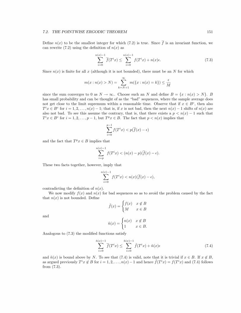
7.2. THE POINTWISE ERGODIC THEOREM 151
Define n(x) to be the smallest integer for which (7.2) is true. Since f is an invariant function, wecan rewrite (7.2) using the definition of n(x) as
n(x)−1∑i=0
f(T ix) ≤n(x)−1∑i=0
f(T ix) + n(x)ε. (7.3)
Since n(x) is finite for all x (although it is not bounded), there must be an N for which
m(x : n(x) > N) =∞∑
k=N+1
m(x : n(x) = k) ≤ ε
M
since the sum converges to 0 as N → ∞.. Choose such an N and define B = x : n(x) > N. Bhas small probability and can be thought of as the “bad” sequences, where the sample average doesnot get close to the limit supremum within a reasonable time. Observe that if x ∈ Bc, then alsoT ix ∈ Bc for i = 1, 2, . . . , n(x)− 1; that is, if x is not bad, then the next n(x)− 1 shifts of n(x) arealso not bad. To see this assume the contrary, that is, that there exists a p < n(x) − 1 such thatT ix ∈ Bc for i = 1, 2, . . . , p− 1, but T px ∈ B. The fact that p < n(x) implies that
p−1∑i=0
f(T ix) < p(f(x)− ε)
and the fact that T px ∈ B implies that
n(x)−1∑i=p
f(T ix) < (n(x)− p)(f(x)− ε).
These two facts together, however, imply that
n(x)−1∑i=0
f(T ix) < n(x)(f(x)− ε),
contradicting the definition of n(x).We now modify f(x) and n(x) for bad sequences so as to avoid the problem caused by the fact
that n(x) is not bounded. Define
f(x) =
f(x) x 6∈ BM x ∈ B
and
n(x) =
n(x) x 6∈ B1 x ∈ B.
Analogous to (7.3) the modified functions satisfy
n(x)−1∑i=0
f(T ix) ≤n(x)−1∑i=0
f(T ix) + n(x)ε (7.4)
and n(x) is bound above by N . To see that (7.4) is valid, note that it is trivial if x ∈ B. If x 6∈ B,as argued previously T ix 6∈ B for i = 1, 2, . . . , n(x)− 1 and hence f(T ix) = f(T ix) and (7.4) followsfrom (7.3).

152 CHAPTER 7. ERGODIC THEOREMS
Observe for later reference that∫f(x) dm(x) =
∫Bcf(x) dm(x) +
∫B
f(x) dm(x)
≤∫Bcf(x) dm(x) +
∫B
M dm(x)
≤∫f(x) dm(x) +Mm(B) ≤
∫f(x) dm(x) + ε, (7.5)
where we have used the fact that f was assumed positive in the second inequality.We now break up the sequence into nonoverlapping blocks such that within each block the sample
average of f is close to the limit supremum. Since the overall sample average is a weighted sum of thesample averages for each block, this will give a long term sample average near the limit supremum.To be precise, choose an L so large that NM/L < ε and inductively define nk(x) by n0(x) = 0 and
nk(x) = nk−1(x) + n(Tnk−1(x)x).
Let k(x) be the largest k for which nk(x) ≤ L− 1, that is, the number of the blocks in the length Lsequence. Since
L−1∑i=0
f(T ix) =k(x)∑k=1
nk(x)−1∑i=nk−1(x)
f(T ix) +L−1∑
i=nk(x)(x)
f(T ix),
we can apply the bound of (7.4) to each of the k(x) blocks, that is, each of the previous k(x) innersums, to obtain
L−1∑i=0
f(T ix) ≤L−1∑i=0
f(T ix) + Lε+ (N − 1)M,
where the final term overbounds the values in the final block by M and where the nonnegativity of fallows the sum to be extended to L− 1. We can now integrate both sides of the preceding equation,divide by L, use the stationarity of m, and apply (7.5) to obtain∫
f dm ≤∫f dm+ ε+
(N − 1)ML
≤∫f dm+ 3ε, (7.6)
which proves the left-hand inequality of (7.1) for the case where f is nonnegative and f is boundedsince ε is arbitrary.
Next suppose that f is not bounded. Define for any M the “clipped” function fM (x) =min(f(x),M) and replace f by fM from (7.2) in the preceding argument. Since fM is also in-variant, the identical steps then lead to∫
fM dm ≤∫f dm.
Taking the limit as M →∞ then yields the desired left-hand inequality of (7.1) from the monotoneconvergence theorem.
To prove the right-hand inequality of (7.1) we proceed in a similar manner. Fix ε > 0 and definen(x) to be the least positive integer for which
1n
n−1∑i=0
f(T ix) ≤ f(x) + ε

7.2. THE POINTWISE ERGODIC THEOREM 153
and define B = x : n(x) > N, where N is chosen large enough to ensure that∫B
f(x) dm(x)ε.
This time define
f(x) =
f(x) x 6∈ B0 x ∈ B.
and
n(x) =
n(x) x 6∈ B1 x ∈ B
and proceed as before.This proves (7.1) and thereby shows that the sample averages of all m-integrable functions
converge. From Corollary 6.6.1, the limit must be the conditional expectations. (The fact thatthe limits must be conditional expectations can also be deduced from the preceding arguments byrestricting the integrations to invariant sets.) 2
Combining the theorem with the results of previous chapter immediately yields the followingcorollaries.
Corollary 7.2.1 If a dynamical system (Ω,B,m, T ) is AMS with stationary mean m and if thesequence n−1
∑n−1i=0 fT
i is uniformly integrable with respect to m, then the following limit is truem-a.e., m-a.e., and in L1(m):
limn→∞
1n
n−1∑i=0
fT i = f = Em(f |I),
where I is the sub-σ-field of invariant events, and
Emf = Ef = Ef.
If in addition the system is ergodic, then
limn→∞
1n
n−1∑i=0
fT i = Em(f)
in both senses.
Corollary 7.2.2 A necessary and sufficient condition for a dynamical system to possess ergodicproperties with respect to all bounded measurements is that it be AMS.
Exercises
1. Suppose that m is stationary and that g is a measurement that has the form g = f − fT forsome measurement f ∈ L2(m). Show that < g >n has an L2(m) limit as n → ∞. Show thatany such g is orthogonal to I∈, the subspace of all square-integrable invariant measurements;that is, E(gh) = 0 for all h ∈ I∈. Suppose that gn is a sequence of functions of this form thatconverges to a measurement r in L2(m). Show that < r >n converges in L2(m).

154 CHAPTER 7. ERGODIC THEOREMS
2. Suppose that < f >n converges in L2(m) for a stationary measure m. Show that the sampleaverages look increasingly like invariant functions in the sense that
|| < f >n − < f >n T || →n→∞ 0.
3. Show that if p and m are two stationary and ergodic measures, then they are either identicalor singular in the sense that there is an event F for which p(F ) = 1 and m(F ) = 0.
4. Show that if p and m are distinct stationary and ergodic processes and λ ∈ (0, 1), then themixture process λp+ (1− λ)m is not ergodic.
7.3 Block AMS Processes
Given a dynamical system (Ω,B,m, T ) or a corresponding source Xn, one may be interestedin the ergodic properties of successive blocks or vectors XN
nN = (XnN , XnN+1, . . . , X(n+1)N−1) or,equivalently, in the N -shift TN . For example, in communication systems one may use block codesthat parse the input source into N -tuples and then map these successive nonoverlapping blocks intocodewords for transmission. A natural question is whether or not a source being AMS with respectto T (T -AMS) implies that it is also TN -AMS or vice versa. This section is devoted to answeringthis question.
First note that if a source is T -stationary, then it is clearly N -stationary (stationary with respectto TN ) since for any event F m(T−NF ) = m(T−N−1F ) = . . . = m(F ). The converse is not true,however, since, for example, a process that produces a single sequence that is periodic with periodN is N -stationary but not stationary. The following lemma, which is a corollary to the ergodictheorem, provides a needed step for treating AMS systems.
Lemma 7.3.1 If µ and η are probability measures on (Ω,B) and if η is T -stationary and asymp-totically dominates µ (with respect to T ), then µ is T -AMS.
Proof: If η is stationary, then from the ergodic theorem it possesses ergodic properties with respectto all bounded measurements. Since it asymptotically dominates µ, µ must also possesses ergodicproperties with respect to all bounded measurements from Corollary 6.3.5. From Theorem 6.2.1, µmust therefore be AMS. 2
The principal result of this section is the following:
Theorem 7.3.1 If a system (Ω,B,m, T ) is TN -AMS for any positive integer N , then it is TN -AMSfor all integers N .
Proof: Suppose first that the system is TN -AMS and let mN denote its N -stationary mean. Thenfor any event F
limn→∞
1n
n−1∑i=0
m(T−iNT−jF ) = mN (T−jF ); j = 0, 1, . . . , N − 1. (7.7)
We then have
1N
N−1∑j=0
limn→∞
1n
n−1∑i=0
m(T−iNT−jF ) = limn→∞
1nN
N−1∑j=0
n−1∑i=0
m(T−iNT−jF )
= limn→∞
1n
n−1∑i=0
m(T−iF ), (7.8)
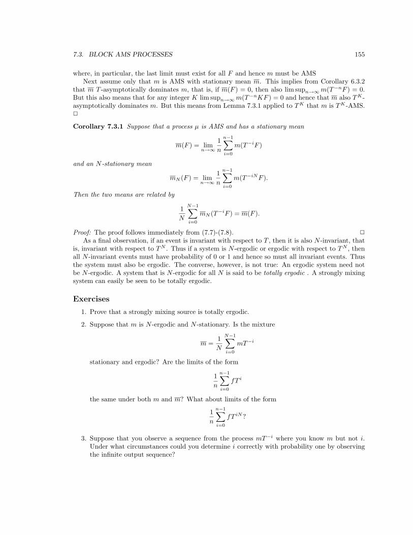
7.3. BLOCK AMS PROCESSES 155
where, in particular, the last limit must exist for all F and hence m must be AMSNext assume only that m is AMS with stationary mean m. This implies from Corollary 6.3.2
that m T -asymptotically dominates m, that is, if m(F ) = 0, then also lim supn→∞m(T−nF ) = 0.But this also means that for any integer K lim supn→∞m(T−nKF ) = 0 and hence that m also TK-asymptotically dominates m. But this means from Lemma 7.3.1 applied to TK that m is TK-AMS.2
Corollary 7.3.1 Suppose that a process µ is AMS and has a stationary mean
m(F ) = limn→∞
1n
n−1∑i=0
m(T−iF )
and an N -stationary mean
mN (F ) = limn→∞
1n
n−1∑i=0
m(T−iNF ).
Then the two means are related by
1N
N−1∑i=0
mN (T−iF ) = m(F ).
Proof: The proof follows immediately from (7.7)-(7.8). 2
As a final observation, if an event is invariant with respect to T , then it is also N -invariant, thatis, invariant with respect to TN . Thus if a system is N -ergodic or ergodic with respect to TN , thenall N -invariant events must have probability of 0 or 1 and hence so must all invariant events. Thusthe system must also be ergodic. The converse, however, is not true: An ergodic system need notbe N -ergodic. A system that is N -ergodic for all N is said to be totally ergodic . A strongly mixingsystem can easily be seen to be totally ergodic.
Exercises
1. Prove that a strongly mixing source is totally ergodic.
2. Suppose that m is N -ergodic and N -stationary. Is the mixture
m =1N
N−1∑i=0
mT−i
stationary and ergodic? Are the limits of the form
1n
n−1∑i=0
fT i
the same under both m and m? What about limits of the form
1n
n−1∑i=0
fT iN?
3. Suppose that you observe a sequence from the process mT−i where you know m but not i.Under what circumstances could you determine i correctly with probability one by observingthe infinite output sequence?

156 CHAPTER 7. ERGODIC THEOREMS
7.4 The Ergodic Decomposition
In this section we find yet another characterization of the limiting sample averages of the ergodictheorem. We use the ergodic properties to show that the stationary mean of an AMS measure thatdescribes the limiting sample averages can be considered as a mixture of ergodic stationary measures.Roughly speaking, if we view the outputs of an AMS system, then we are viewing the outputs of anergodic system, but we do not know a priori which one. If we view the limiting sample frequencies,however, we can determine the ergodic source being seen.
We have seen that if a dynamical system (Ω,B,m, T ) is AMS with stationary mean m and hencehas ergodic properties with respect to all indicator functions, then the limiting relative frequencies(the sample averages of the indicator functions) are conditional probabilities, < 1F >= m(F |I),where I is the sigma-field of invariant events. In addition, if the alphabet is standard, one can selecta regular version of the conditional probability and hence using iterated expectation one can considerthe stationary mean distribution m as a mixture of measures m(·|I)(x); x ∈ Ω. In this section weshow that almost all of these measures are both stationary and ergodic, and hence the stationarymean of an AMS system, which describes the sample average behavior of the system, can be writtenas a mixture of stationary and ergodic distributions. Intuitively, observing the asymptotic sampleaverages of an AMS system is equivalent to observing the same measurements for a stationary andergodic system that is an ergodic component of the stationary mean, but we may not know in advancewhich ergodic component is being observed. This result is known as the ergodic decomposition and itis due in various forms to Von Neumann [71], Rohlin [60], Kryloff and Bogoliouboff [42], and Oxtoby[53]. The development here most closely parallels that of Oxtoby. (See also Gray and Davisson [23]for the simple special case of discrete alphabet processes.)
Although we could begin with Theorem 6.6.1, which characterizes the limiting relative frequenciesas conditional probabilities, and then use Theorem 5.7.1 to choose a regular version of the conditionalprobability, it is more instructive to proceed in a direct fashion by assuming ergodic properties. Inaddition, this yields a stronger result wherein the decomposition is determined by the properties ofthe points themselves and not the underlying measure; that is, the same decomposition works forall AMS measures.
Let (Ω,B,m, T ) be a dynamical system and assume that (Ω,B) is a standard measurable spacewith a countable generating set F .
For each event F define the invariant set G(F ) = x : limn→∞ < 1F >n (x) exists and denotethe invariant limit by < 1F >. Define the set
G(F) =⋂F∈F
G(F ),
the set of points x for which the limiting relative frequencies of all generating events exist. We shallcall G(F) the set of generic points.
Thus for any x ∈ G(F)
limn→∞
n−1∑i=0
1F (T ix) = 1F (x); all F ∈ F .
Observe that membership in G(F) is determined strictly by properties of the points and notby an underlying measure. If m has ergodic properties with respect to the class of all indicatorfunctions, i.e., if it is AMS, then clearly m(G(F )) = 1 for any event F and hence we also have forthe countable intersection that m(G(F)) = 1. If x ∈ G(F), then the set function Px defined by
Px(F ) = 1F (x) ;F ∈ F

7.4. THE ERGODIC DECOMPOSITION 157
is nonnegative, normalized, and finitely additive on F from the properties of sample averages. Sincethe space is standard, this set function extends to a probability measure, which we shall also denoteby Px, on (Ω,B). Thus we easily obtain that every generic point induces a probability measure Pxand hence also a dynamical system (Ω,B, Px, T ) via its convergent relative frequencies. For x not inG(F) we can simply fix Px as some fixed arbitrary stationary and ergodic measure p∗.
We now confine interest to AMS systems so that the set of generic sequences will have probabilityone. Then Px(F ) =< 1F > (x) almost everywhere and Px(F ) = m(F |I)(x) for all x in a set of mmeasure one. Since this is true for any event F , we can define the countable intersection
H = x : Px(F ) = m(F |I) all F ∈ F
and infer that m(H) = 1. Thus with probability one under m the two measures Px and m(·|I)(x)agree on F and hence are the same. Thus from the properties of conditional probability and condi-tional expectation
m(F ∩D) =∫D
Px(F )dm, all D ∈ I, (7.9)
and if f is in L1(m), then ∫D
f dm =∫D
(∫f(y) dPx(y))dm, all D ∈ I. (7.10)
Thus choosing D = Ω we can interpret (7.9) as stating that the stationary mean m is a mixture ofthe probability measures Px and (7.10) as stating that the expectation of measurements with respectto the stationary mean can be computed (using iterated expectation) in two steps: First find theexpectations with respect to the components Px for all x and then take the average. Such mixtureand average representations will be particularly useful because, as we shall show, the componentmeasures are both stationary and ergodic with probability one. For focus and motivation, we nextstate the principal result of this section–the ergodic decomposition theorem–which makes this notionrigorous in a useful form. The remainder of the section is then devoted to the proof of this theoremvia a sequence of lemmas that are of some interest in their own right.
Theorem 7.4.1 (The Ergodic Decomposition)Given a standard measurable space (Ω,B), let F denote a countable generating field. Given a
transformation T : Ω→ Ω define the set of generic sequences
G(F) = x : limn→∞
< 1F >n (x) exists all F ∈ F.
For each x ∈ G(F) let Px denote the measure induced by the limiting relative frequencies. Define theset E ⊂ G(F) by E = x : Px is stationary and ergodic. Define the stationary and ergodic measurespx by px = Px for x ∈ E and otherwise px = p∗, some fixed stationary and ergodic measure. (Notethat so far all definitions involve properties of the points only and not of any underlying measure.)We shall refer to the collection of measures px;x ∈ Ω as the ergodic decomposition. We havethen that
(a) E is an invariant measurable set,
(b) px(F ) = pTx(F ) for all points x ∈ Ω and events F ∈ B,
(c) If m is an AMS measure with stationary mean m, then
m(E) = m(E) = 1, (7.11)

158 CHAPTER 7. ERGODIC THEOREMS
(d) for any F ∈ B
m(F ) =∫px(F )dm(x) =
∫px(F )dm(x), (7.12)
(e) and if f ∈ L1(m), then so is∫f dpx and∫
f dm =∫
(∫fdpx)dm(x). (7.13)
(g) In addition, given any f ∈ L1(m), then
limn→∞
n−1n−1∑i=0
f(T ix) = Epxf,m− a.e. and m− a.e. (7.14)
Comment: The final result is extremely important for both mathematics and intuition: Say thata system source is AMS and that f is integrable with respect to the stationary mean; e.g., f ismeasurable and bounded and hence integrable with respect to any measure. Then with probabilityone a point will be produced such that the limiting sample average exists and equals the expectationof the measurement with respect to the stationary and ergodic measure induced by the point. Thusif a system is AMS, then the limiting sample averages will behave as if they were in fact produced bya stationary and ergodic system. These ergodic components are determined by the points themselvesand not the underlying measure; that is, the same collection works for all AMS measures.Proof: We begin the proof by observing that the definition of Px implies that
PTx(F ) = 1F (Tx) = 1F (x) = Px(F ); all F ∈ F ; all x ∈ G(F) (7.15)
since limiting relative frequencies are invariant. Since PTx and Px agree on generating field events,however, they must be identical. Since we will select the px to be the Px on a subset of G(F), thisproves (b) for x ∈ E.
Next observe that for any x ∈ G(F) and F ∈ F
Px(F ) = 1F (x) = limn→∞
n−1∑i=0
1F (T ix) = limn→∞
n−1∑i=0
1T−1F (T ix) = 1T−1F (x) = Px(T−1F ).
Thus for x ∈ G(F) the measure Px looks stationary, at least on generating events. The followinglemma shows that this is enough to infer that the Px are indeed stationary.
Lemma 7.4.1 A measure m is stationary on (Ω, σ(F)) if and only if m(T−1F ) = m(F ) for allF ∈ F .
Proof: Both m and mT−1 are measures on the same space, and hence they are equal if and only ifthey agree on a generating field. 2
Note in passing that no similar countable description of an AMS measure is known, that is, iflimn→∞ n−1
∑n−1i=0 m(T−iF ) converges for all F in a generating field, it does not follow that the
measure is AMS.As before let E denote the subset of G(F) consisting of all of the points x for which Px is ergodic.
From Lemma 6.7.4, the definition of Px, and the stationarity of the Px we can write E as
E = x : x ∈ G(F); limn→∞
n−1n−1∑i=0
Px(T−iF ∩ F ) = Px(F )2, all F ∈ F.

7.4. THE ERGODIC DECOMPOSITION 159
Since the probabilities Px are measurable functions, the set E where the given limit exists and hasthe given value is also measurable. Since Px(F ) = PTx(F ), the set is also invariant. This proves (a)of the theorem. We have already proved (b) for x ∈ E. For x 6∈ E we have that px = p∗. Since E isinvariant, we also know that Tx 6∈ E and hence also pTx = p∗ so that pTx = px.
We now consider an AMS measure m. Although Lemma 6.7.4 provided a countable descriptionof ergodicity that was useful to prove that the collection of all points inducing ergodic measures isan event, the following lemma provides another countable description of ergodicity that is useful forcomputing the probability of the set E.
Lemma 7.4.2 Let (Ω, σ(F),m, T ) be an AMS dynamical system with stationary mean m. Definethe sets
G(F,m) = x : limn→∞
1n
n−1∑i=0
1F (T ix) = m(F );F ∈ F .
Thus G(F,m) is the set of sequences for which the limiting relative frequency exists for all events Fin the generating field and equals the probability of the event under the stationary mean. Define also
G(F ,m) =⋂F∈F
G(F,m).
A necessary and sufficient condition for m to be ergodic is that m(G(F ,m)) = 1.
Comment: The lemma states that an AMS measure m is ergodic if and only if it places all of itsprobability on the set of generic points that induce m through their relative frequencies.Proof: If m is ergodic then < 1F >= m(F )m-a.e. for all F and the result follows immediately.Conversely, if m(G(F ,m)) = 1 then also m(G(F ,m)) = 1 since the set is invariant. Thus integratingto the limit using the dominated convergence theorem yields
limn→∞
n−1n−1∑i=0
m(T−iF ∩ F ) =∫G(F,m)
1F ( limn→∞
n−1n−1∑i=0
1FT i)dm
= m(F )2, all F ∈ F ,
which with Lemma 6.7.4 proves that m is ergodic, and hence so is m from Lemma 6.7.2. 2
Proof of the Theorem If we can show that m(E) = 1, then the remainder of the theorem will followfrom (7.9) and (7.10) and the fact that px = m(·|I)(x) m− a.e. From the previous lemma, this willbe the case if with px probability one
1F = px(F ), all F ∈ F ,
or, equivalently, if for all F ∈ F1F = px(F ) px − a.e.
This last equation will hold if for each F ∈ F∫dpx(y)|1F (y)− px(F )|2 = 0.
This relation will hold on a set of x of m probability one if∫dm(x)
∫dpx(y) |1F (y)− px(F )|2 = 0.
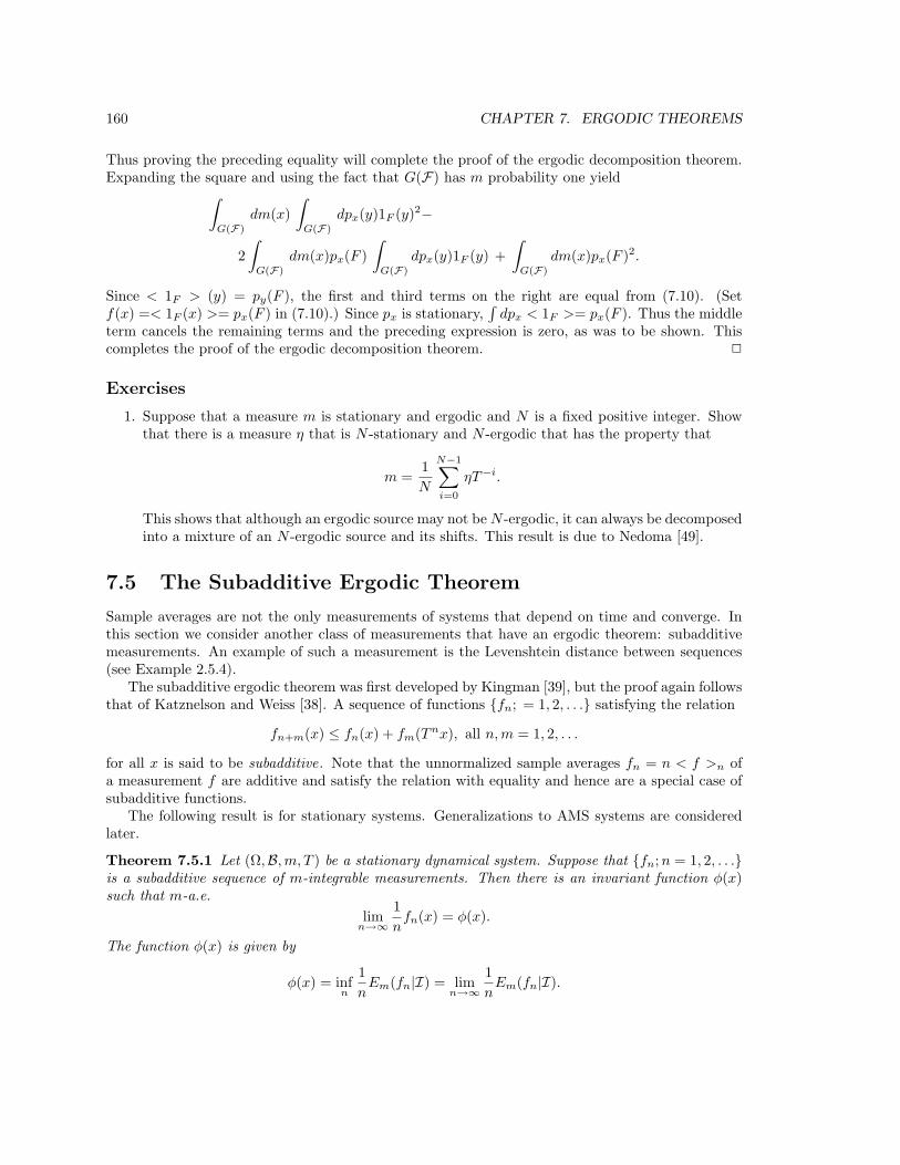
160 CHAPTER 7. ERGODIC THEOREMS
Thus proving the preceding equality will complete the proof of the ergodic decomposition theorem.Expanding the square and using the fact that G(F) has m probability one yield∫
G(F)
dm(x)∫G(F)
dpx(y)1F (y)2−
2∫G(F)
dm(x)px(F )∫G(F)
dpx(y)1F (y) +∫G(F)
dm(x)px(F )2.
Since < 1F > (y) = py(F ), the first and third terms on the right are equal from (7.10). (Setf(x) =< 1F (x) >= px(F ) in (7.10).) Since px is stationary,
∫dpx < 1F >= px(F ). Thus the middle
term cancels the remaining terms and the preceding expression is zero, as was to be shown. Thiscompletes the proof of the ergodic decomposition theorem. 2
Exercises
1. Suppose that a measure m is stationary and ergodic and N is a fixed positive integer. Showthat there is a measure η that is N -stationary and N -ergodic that has the property that
m =1N
N−1∑i=0
ηT−i.
This shows that although an ergodic source may not beN -ergodic, it can always be decomposedinto a mixture of an N -ergodic source and its shifts. This result is due to Nedoma [49].
7.5 The Subadditive Ergodic Theorem
Sample averages are not the only measurements of systems that depend on time and converge. Inthis section we consider another class of measurements that have an ergodic theorem: subadditivemeasurements. An example of such a measurement is the Levenshtein distance between sequences(see Example 2.5.4).
The subadditive ergodic theorem was first developed by Kingman [39], but the proof again followsthat of Katznelson and Weiss [38]. A sequence of functions fn; = 1, 2, . . . satisfying the relation
fn+m(x) ≤ fn(x) + fm(Tnx), all n,m = 1, 2, . . .
for all x is said to be subadditive. Note that the unnormalized sample averages fn = n < f >n ofa measurement f are additive and satisfy the relation with equality and hence are a special case ofsubadditive functions.
The following result is for stationary systems. Generalizations to AMS systems are consideredlater.
Theorem 7.5.1 Let (Ω,B,m, T ) be a stationary dynamical system. Suppose that fn;n = 1, 2, . . .is a subadditive sequence of m-integrable measurements. Then there is an invariant function φ(x)such that m-a.e.
limn→∞
1nfn(x) = φ(x).
The function φ(x) is given by
φ(x) = infn
1nEm(fn|I) = lim
n→∞
1nEm(fn|I).

7.5. THE SUBADDITIVE ERGODIC THEOREM 161
Most of the remainder of this section is devoted to the proof of the theorem. On the way somelemmas giving properties of subadditive functions are developed. Observe that since the conditionalexpectations with respect to the σ-field of invariant events are themselves invariant functions, φ(x)is invariant as claimed.
Since the functions are subadditive,
Em(fn+m|I) ≤ Em(fn|I) + Em(fmTn|I).
From the ergodic decomposition theorem, however, the third term is EPx(fmTn) = EPx(fm) sincePx is a stationary measure with probability one. Thus we have with probability one that
Em(fn+m|I)(x) ≤ Em(fn|I)(x) + Em(fm|I)(x).
For a fixed x, the preceding is just a sequence of numbers, say ak, with the property that
an+k ≤ an + ak.
A sequence satisfying such an inequality is said to be subadditive. The following lemma (due toHammersley and Welch [32]) provides a key property of subadditive sequences.
Lemma 7.5.1 If an;n = 1, 2, . . . is a subadditive sequence, then
limn→∞
ann
= infn≥1
ann,
where if the right-hand side is −∞, the preceding means that an/n diverges to −∞.
Proof: First observe that if an is subadditive, for any k, n
akn ≤ an + a(k−1)n ≤ an + an + a(k−2)n ≤ . . . ≤ kan. (7.16)
Call the infimum γ and first consider the case where it is finite. Fix ε > 0 and choose a positiveinteger N such that N−1aN < γ + ε. Define b = max1≤k≤3N−1 ak. For each n ≥ 3N there is aunique integer k(n) for which (k(n) + 2)N ≤ n < (k(n) + 3)N . Since the sequence is subadditive,an ≤ ak(n)N + a(n−k(n)N). Since n− k(n)N < 3N by construction, an−k(n)N ≤ b and therefore
γ ≤ ann≤ak(n)N + b
n.
Using (7.16) this yields
γ ≤ ann≤ k(n)aN
n+b
n≤ k(n)N
n
aNN
+b
n≤ k(n)N
n(γ + ε) +
b
n.
By construction k(n)N ≤ n− 2N ≤ n and hence
γ ≤ ann≤ γ + ε+
b
n.
Thus given an ε, choosing n0 large enough yields γ ≤ n−1an ≤ γ + 2ε for all n > n0, proving thelemma. If γ is −∞, then for any positive M we can choose n so large that n−1an ≤ −M . Proceedingas before for any ε there is an n0 such that if n ≥ n0, then n−1an ≤ −M + ε. Since M is arbitrarilybig and ε arbitrarily small, n−1an goes to −∞. 2

162 CHAPTER 7. ERGODIC THEOREMS
Returning to the proof of the theorem, the preceding lemma implies that with probability one
φ(x) = infn≥1
1nEm(fn|I)(x) = lim
n→∞
1nEm(fn|I)(x).
As in the proof of the ergodic theorem, define
f(x) = lim supn→∞
1nfn(x)
andf(x) = lim inf
n→∞
1nfn(x).
Lemma 7.5.2 Given a subadditive function fn(x); = 1, 2, . . ., f and f as defined previously areinvariant functions m-a.e.
Proof: From the definition of subadditive functions
f1+n(x) ≤ f1(x) + fn(Tx)
and hencefn(Tx)n
≥ 1 + n
n
f1+n(x)1 + n
− f1(x)n
.
Taking the limit supremum yields f(Tx) ≥ f(x). Since m is stationary, EmfT = Emf and hencef(x) = f(Tx) m-a.e. The result for f follows similarly. 2
We now tackle the proof of the theorem. It is performed in two steps. The first uses the usualergodic theorem and subadditivity to prove that f ≤ φ a.e. Next a construction similar to that ofthe proof of the ergodic theorem is used to prove that f = φ a.e., which will complete the proof.
As an introduction to the first step, observe that since the measurements are subadditive
1nfn(x) ≤ 1
n
n−1∑i=0
f1(T ix).
Since f1 ∈ L1(m) for the stationary measure m, we know immediately from the ergodic theoremthat
f(x) ≤ f1(x) = Em(f1|I). (7.17)
We can obtain a similar bound for any of the fn by breaking it up into fixed size blocks of length,say N and applying the ergodic theorem to the sum of the fN . Fix N and choose n ≥ N . For eachi = 0, 1, 2, . . . , N − 1 there are integers j, k such that n = i + jN + k and 1 ≤ k < N . Hence usingsubadditivity
fn(x) ≤ fi(x) +j−1∑l=0
fN (T lN+ix) + fk(T jN+ix).
Summing over i yields
Nfn(x) ≤N−1∑i=0
fi(x) +jN−1∑l=0
fN (T lx) +N−1∑i=0
fn−i−jN (T jN+ix),

7.5. THE SUBADDITIVE ERGODIC THEOREM 163
and hence
1nfn(x) ≤ 1
nN
jN−1∑l=0
fN (T lx) +1nN
N−1∑i=0
fi(x) +1nN
N−1∑i=0
fn−i−jN (T jN+ix).
As n → ∞ the middle term on the right goes to 0. Since fN is assumed integrable with respect tothe stationary measure m, the ergodic theorem implies that the leftmost term on the right tendsto N−1 < fN >. Intuitively the rightmost term should also go to zero, but the proof is a bit moreinvolved. The rightmost term can be bound above as
1nN
N−1∑i=0
|fn−i−jN (T jN+ix)| ≤ 1nN
N−1∑i=0
N∑l=1
|fl(T jN+ix)|
where j depends on n (the last term includes all possible combinations of k in fk and shifts). Definethis bound to be wn/n. We shall prove that wn/n tends to 0 by using Corollary 4.6.1, that is, byproving that
∞∑n=0
m(wnn
> ε) <∞. (7.18)
First note that since m is stationary,
wn =1N
N−1∑i=0
N∑l=1
|fl(T jN+ix)|
has the same distribution as
w =1N
N−1∑i=0
N∑l=1
|fl(T ix)|.
Thus we will have proved (7.18) if we can show that
∞∑n=0
m(w > nε) <∞. (7.19)
To accomplish this we need a side result, which we present as a lemma.
Lemma 7.5.3 Given a nonnegative random variable X defined on a probability space (Ω,B,m),
∞∑n=1
m(X ≥ n) ≤ EX.
Proof:
EX =∞∑n=1
E(X|X ∈ [n− 1, n))m(X ∈ [n− 1, n))
≥∞∑n=1
(n− 1)m(X ∈ [n− 1, n))
=∞∑n=1
nm(X ∈ [n− 1, n))− 1.

164 CHAPTER 7. ERGODIC THEOREMS
By rearranging terms the last sum can be written as
∞∑n=0
m(X ≥ n),
which proves the lemma. 2
Applying the lemma to the left side of (7.19) yields
∞∑n=0
m(w
ε> n) ≤
∞∑n=0
m(w
ε≥ n) ≤ 1
εEm(w) <∞,
since m-integrability of the fn implies m-integrability of their absolute magnitudes and hence of afinite sum of absolute magnitudes. This proves (7.19) and hence (7.18). Thus we have shown that
f(x) ≤ 1NfN (x) =
1NEm(fN |I)
for all N and hence thatf(x) ≤ φ(x),m− a.e. . (7.20)
This completes the first step of the proof.If φ(x) = −∞, then (7.20) completes the proof since the desired limit then exists and is −∞.
Hence we can focus on the invariant set G = x : φ(x) > −∞. Define the event GM = x : φ(x) ≥−M. We shall show that for all M ∫
GM
f dm ≥∫GM
φdm, (7.21)
which with (7.20) proves that f = φ on GM . We have, however, that
G =∞⋃M=1
GM .
Thus proving that f = φ on all GM also will prove that f = φ on G and complete the proof of thetheorem.
We now proceed to prove (7.21) and hence focus on x in GM and hence only x for whichφ(x) ≥ −M . We proceed as in the proof of the ergodic theorem. Fix an ε > 0 and define f
M=
max(f,−M − 1). Observe that this implies that
φ(x) ≥ fM
(x), all x. (7.22)
Define n(x) as the smallest integer n ≥ 1 for which n−1fn(x) ≤ fM
(x) + ε. Define B = x : n(x) >N and choose N large enough so that∫
B
(|f1(x)|+M + 1) dm(x) < ε. (7.23)
Define the modified functions as before:
fM
(x) =
fM
(x) x 6∈ Bf1(x) x ∈ B

7.5. THE SUBADDITIVE ERGODIC THEOREM 165
and
n(x) =
n(x) x 6∈ B1 x ∈ B.
From (7.23) ∫fMdm =
∫BcfMdm+
∫B
fMdm
=∫BcfMdm+
∫B
f1 dm
≤∫BcfMdm+
∫B
|f1| dm
≤∫BcfMdm+ ε−
∫B
(M + 1) dm
≤∫BcfMdm+ ε+
∫B
fMdm
≤∫fMdm+ ε. (7.24)
Since fM
is invariant,
fn(x)(x) ≤n(x)−1∑i=0
fM
(T ix) + n(x)ε
and hence also
fn(x)(x) ≤n(x)−1∑i=0
fM
(T ix) + n(x)ε
Thus for L > N
fL(x) ≤L−1∑i=0
fM
(T ix) + Lε+N(M − 1) +L−1∑
i=L−N|f1(T ix)|.
Integrating and dividing by L results in∫φ(x) dm(x) ≤
∫1LfL(x) dm(x) =
∫1LfL(x) dm(x)
≤∫fM
(x) dm(x) + ε+N(M + 1)
L+N
L
∫|f1(x)| dm(x).
Letting L→∞ and using (7.24) yields∫φ(x) dm(x) ≤
∫fM
(x) dm(x).
From (7.22), however, this can only hold if in fact fM
(x) = φ(x) a.e. This implies, however, thatf(x) = φ(x) a.e. since the event f(x) 6= f
M(x) implies that f
M(x) = −M − 1 which can only
happen with probability 0 from (7.22) and the fact that fM
(x) = φ(x) a.e. This completes the proofof the subadditive ergodic theorem for stationary measures. 2
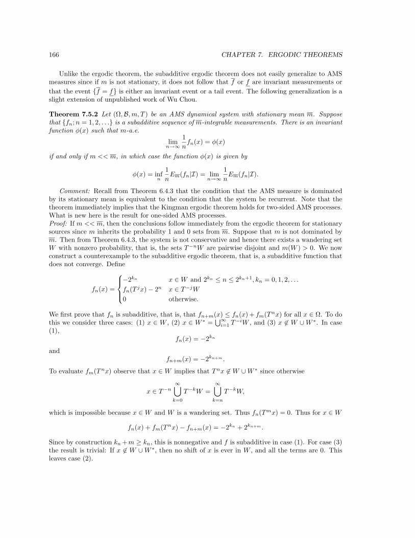
166 CHAPTER 7. ERGODIC THEOREMS
Unlike the ergodic theorem, the subadditive ergodic theorem does not easily generalize to AMSmeasures since if m is not stationary, it does not follow that f or f are invariant measurements orthat the event f = f is either an invariant event or a tail event. The following generalization is aslight extension of unpublished work of Wu Chou.
Theorem 7.5.2 Let (Ω,B,m, T ) be an AMS dynamical system with stationary mean m. Supposethat fn;n = 1, 2, . . . is a subadditive sequence of m-integrable measurements. There is an invariantfunction φ(x) such that m-a.e.
limn→∞
1nfn(x) = φ(x)
if and only if m << m, in which case the function φ(x) is given by
φ(x) = infn
1nEm(fn|I) = lim
n→∞
1nEm(fn|I).
Comment: Recall from Theorem 6.4.3 that the condition that the AMS measure is dominatedby its stationary mean is equivalent to the condition that the system be recurrent. Note that thetheorem immediately implies that the Kingman ergodic theorem holds for two-sided AMS processes.What is new here is the result for one-sided AMS processes.Proof: If m << m, then the conclusions follow immediately from the ergodic theorem for stationarysources since m inherits the probability 1 and 0 sets from m. Suppose that m is not dominated bym. Then from Theorem 6.4.3, the system is not conservative and hence there exists a wandering setW with nonzero probability, that is, the sets T−nW are pairwise disjoint and m(W ) > 0. We nowconstruct a counterexample to the subadditive ergodic theorem, that is, a subadditive function thatdoes not converge. Define
fn(x) =
−2kn x ∈W and 2kn ≤ n ≤ 2kn+1, kn = 0, 1, 2, . . .fn(T jx)− 2n x ∈ T−jW0 otherwise.
We first prove that fn is subadditive, that is, that fn+m(x) ≤ fn(x) + fm(Tnx) for all x ∈ Ω. To dothis we consider three cases: (1) x ∈ W , (2) x ∈ W ∗ =
⋃∞i=1 T
−iW , and (3) x 6∈ W ∪W ∗. In case(1),
fn(x) = −2kn
andfn+m(x) = −2kn+m .
To evaluate fm(Tnx) observe that x ∈W implies that Tnx 6∈W ∪W ∗ since otherwise
x ∈ T−n∞⋃k=0
T−kW =∞⋃k=n
T−kW,
which is impossible because x ∈W and W is a wandering set. Thus fn(Tmx) = 0. Thus for x ∈W
fn(x) + fm(Tnx)− fn+m(x) = −2kn + 2kn+m .
Since by construction kn+m ≥ kn, this is nonnegative and f is subadditive in case (1). For case (3)the result is trivial: If x 6∈ W ∪W ∗, then no shift of x is ever in W , and all the terms are 0. Thisleaves case (2).

7.5. THE SUBADDITIVE ERGODIC THEOREM 167
Suppose now that x ∈ T−jW for some k. Then
fn+m(x) = fn+m(T jx)− 2n+m = −2kn+m − 2n+m,
andfn(x) = fn(T jx)− 2n = −2kn − 2n.
For the final term there are two cases. If n > j, then analogously to case (1) x ∈ T−jW implies thatTnx 6∈W ∪W ∗ since otherwise
x ∈ T−n∞⋃k=0
T−kW =∞⋃k=n
T−kW,
which is impossible since W is a wandering set and hence x cannot be in both T−jW and in⋃∞k=n T
−kW since n > j. If n ≤ j, then
fm(Tnx) = fm(T jx)− 2m = −2km − 2m.
Therefore if n > j,
fn(x) + fm(Tnx)− fn+m(x) = −2kn − 2n + 0 + 2kn+m + 2n+m ≥ 0.
If n ≤ j then
fn(x) + fm(Tnx)− fn+m(x) = −2kn − 2n − 2km − 2m + 2kn+m + 2n+m.
Suppose that n ≥ m ≥ 1, then
2n+m − 2n − 2m = 2n(2m − 1− 2−|n−m|) ≥ 0.
Similarly, since then kn ≥ km, then
2kn+m − 2kn − 2km = 2kn(2kn+m−kn − 1− 2−|kn−km| ≥ 0.
Similar inequalities follow when n ≤ m, proving that fn is indeed subadditive on Ω.We now complete the proof. The event W has nonzero probability, but if x ∈W , then
limn→∞
12nf2n(x) = lim
n→∞
−2n
2n= −1
whereas
limn→∞
12n − 1
f2n−1(x) = limn→∞
−2n−1
2n − 1= −1
2
and hence n−1fn does not have a limit on this set of nonzero probability, proving that the subadditiveergodic theorem does not hold in this case. 2

168 CHAPTER 7. ERGODIC THEOREMS

Chapter 8
Process Metrics and the ErgodicDecomposition
8.1 Introduction
Given two probability measures, say p and m, on a common probability space, how different ordistant from each other are they? Similarly, given two random processes with distributions p and m,how distant are the processes from each other and what impact does such a distance have on theirrespective ergodic properties? The goal of this final chapter is to develop two quite distinct notionsof the distance d(p,m) between measures or processes and to use these ideas to delve further intothe ergodic properties of processes and the ergodic decomposition. One metric, the distributionaldistance, measures how well the probabilities of certain important events match up for the twoprobability measures, and hence this metric need not have any relation to any underlying metric onthe original sample space. In other words, the metric makes sense even when we are not puttingprobability measures on metric spaces. The second metric, the ρ-distance (rho-bar distance) dependsvery strongly on a metric on the output space of the process and measures distance not by howdifferent probabilities are, but by how well one process can be made to approximate another. Thesecond metric is primarily useful in applications in information theory and statistics. Althoughthese applications are beyond the scope of this book, the metric is presented both for comparisonand because of the additional insight into ergodic properties the metric provides.
Such process metrics are of preliminary interest because they permit the quantitative assessmentof how different two random processes are and how their ergodic properties differ. Perhaps moreimportantly, however, putting a metric on a space of random processes provides a topology forthe space and hence a collection of Borel sets and a measurable space to which we can assignprobability measures. This assignment of a probability measure to a space of processes provides ageneral definition of a mixture process and provides a means of delving more deeply into the ergodicdecomposition of stationary measures developed in the previous chapter.
We have seen from the ergodic decomposition that all AMS measures have a stationary meanthat can be considered as a mixture of stationary and ergodic components. Thus, for example, anystationary measure m can be considered as a mixture of the form
m =∫pxdm(x), (8.1)
169

170 CHAPTER 8. PROCESS METRICS AND THE ERGODIC DECOMPOSITION
which is an abbreviation for
m(F ) =∫px(F ) dm(x), all F ∈ B.
In addition, any m-integrable f can be integrated in two steps as∫f(x) dm(x) =
∫(∫dpx(y)f(y)) dm(x). (8.2)
Thus stationary measures can be considered to be mixtures of stationary and ergodic measures; thatis, a stationary and ergodic measure is randomly selected from some collection and then used. Inother words, we effectively have a probability measure on the space of all stationary and ergodicprobability measures and the first measure is used to select one of the measures of the given class.Alternatively, we have a probability measure on the space of all probability measures on the givenmeasurable space, but this super probability measure assigns probability one to the collection ofergodic and stationary measures. The preceding relations show that both probabilities and expecta-tions of measurements over the resulting mixture can be computed as integrals of the probabilitiesand expectations over the component measures.
In applications of the theory of random processes such as information and communication theory,one is often concerned not only with ordinary functions or measurements, but also with functionalsof probability measures, that is, mappings of the space of probability measures into the real line.Examples include the entropy rate of a dynamical system, the distortion-rate function of a randomprocess with respect to a fidelity criterion, the information capacity of a noisy channel, the raterequired to code a given process with nearly zero reproduction error, the rate required to code agiven process for transmission with a specified fidelity, and the maximum rate of coded informationthat can be transmitted over a noisy channel with nearly zero error probability. (See, for example,the papers and commentary in Gray and Davisson [25].) All of these quantities are functionals ofmeasures: a given process distribution or measure yields a real number as a value of the functional.
Given such a functional of measures, say D(m), it is natural to inquire under what conditionsthe analog of (8.2) for functions might hold, that is, conditions under which
D(m) =∫D(px) dm(x). (8.3)
This is in general a much more difficult issue than before since unlike an ordinary measurement f ,the functional depends on the underlying probability measure. One goal of this chapter to developconditions under which (8.3) holds.
8.2 A Metric Space of Measures
We now focus on spaces of probability measures and on the structure of such spaces. We shall showhow the ergodic decomposition provides an example of a probability measure on such a space. InSection 8.4 we shall study certain functionals defined on this space.
Let (Ω,B) be a measurable space such that B is countably generated (e.g., it is standard). We donot assume any metric structure for Ω. Define P((Ω,B)) as the class of all probability measures on(Ω,B). It is easy to see that P((Ω,B)) is a convex subset of the class of all finite measures on (Ω,B);that is, if m1 and m2 are in P((Ω,B)) and λ ∈ (0, 1), then λm1 + (1− λ)m2 is also in P((Ω,B)).
We can put a variety of metrics on P((Ω,B)) and thereby make it a metric space. This willprovide a notion of closeness of probability measures on the class. It will also provide a Borel field

8.2. A METRIC SPACE OF MEASURES 171
of subsets of P((Ω,B)) on which we can put measures and thereby construct mixtures of measuresin the class.
In this section we consider a type of metric that is not very strong, but will suffice for developingthe ergodic decomposition of affine functionals. In the next section another metric will be considered,but it is tied to the assumption of Ω being itself a metric space and hence applies less generally.
Given any class G = Fi; i = 1, 2, , . . . consisting of a countable collection of events we can definefor any measures p,m ∈ P((Ω,B)) the function
dG(p,m) =∞∑i=1
2−i|p(Fi)−m(Fi)|. (8.4)
If G contains a generating field, then dG is a metric on P((Ω,B)) since from Lemma 1.5.5 twomeasures defined on a common σ-field generated by a field are identical if and only if they agreeon the generating field. We shall always assume that G contains such a field. We shall call such adistance a distributional distance. Usually we will require that G be a standard field and hence thatthe underlying measurable space (Ω,B) is standard. Occasionally, however, we will wish a largerclass G but will not require that it be standard. The different requirements will be required fordifferent results. When the class G is understood from context, the subscript will be dropped.
Let (P(Ω,B), dG) denote the metric space of P((Ω,B)) with the metric dG . A key property ofspaces of probability measures on a fixed measurable space is given in the following lemma.
Lemma 8.2.1 The metric space (P((Ω,B)), dG) of all probability measures on a measurable space(Ω,B) with a countably generated sigma-field is separable if G contains a countable generating field.If also G is standard (as is possible if the underlying measurable space (Ω,B) is standard), then also(P, dG) is complete and hence Polish.
Proof: For each n let An denote the set of nonempty intersection sets or atoms of F1, . . . , Fn, thefirst n sets in G. (These are Ω sets, events in the original space.) For each set G ∈ An choose anarbitrary point xG such that xG ∈ G. We will show that the class of all measures of the form
r(F ) =∑G∈An
pG1F (xG),
where the pG are nonnegative and rational and satisfy∑G∈An
pG = 1,
forms a dense set in P((Ω,B)). Since this class is countable, P((Ω,B)) is separable. Observe that weare approximating all measures by finite sums of point masses. Fix a measure m ∈ (P((Ω,B)), dG)and an ε > 0. Choose n so large that 2−n < ε/2. Thus to match up two measures in d = dG , (8.4)implies that we must match up the probabilities of the first n sets in G since the contribution of theremaining terms is less that 2−n. Define
rn(F ) =∑G∈An
m(G)1F (xG)
and note thatm(F ) =
∑G∈An
m(G)m(F |G),

172 CHAPTER 8. PROCESS METRICS AND THE ERGODIC DECOMPOSITION
where m(F |G) = m(F ∩G)/m(G) is the elementary conditional probability of F given G if m(G) > 0and is arbitrary otherwise. For convenience we now consider the preceding sums to be confined tothose G for which m(G) > 0.
Since the G are the atoms of the first n sets Fi, for any of these Fi either G ⊂ Fi and henceG ∩ Fi = G or G ∩ Fi = ∅. In the first case 1Fi(xG) = m(Fi|G) = 1, and in the second case1Fi(xG) = m(Fi|G) = 0, and hence in both cases
rn(Fi) = m(Fi); i = 1, 2, , . . . , n.
This implies that
d(rn,m) ≤∞∑
i=n+1
2−i = 2−n ≤ ε
2.
Enumerate the atoms of An as Gl; l = 1, 2, . . . , L, where L ≤ 2n. For all l but the last (l = L)pick a rational number pGl such that
m(Gl)− 2−lε
4≤ pGl ≤ m(Gl);
that is, we choose a rational approximation to m(Gl) that is slightly less than m(Gl). We definepGL to force the rational approximations to sum to 1:
pGL = 1−L−1∑l=1
pGl .
Clearly pGL is also rational and
|pGL −m(GL)| = |L−1∑l=1
pGl −L−1∑l=1
m(Gl)|
≤L−1∑l=1
|pGl −m(Gl)|
≤ ε
4
L−1∑l=1
2−l ≤ ε
4.
Thus ∑G∈An
|pG −m(G)| =L−1∑l=1
|pGl −m(Gl)|+ |pGL −m(GL)| ≤ ε
2.
Define now the measure tn by
tn(F ) =∑G∈An
pG1F (xG)
and observe that
d(tn, rn) =n∑i=1
2−i|tn(Fi)− rn(Fi)|
=n∑i=1
2−i|∑G∈An
1Fi(pG −m(G))|
≤n∑i=1
2−i∑G∈An
|pG −m(G)| ≤ ε
4.

8.2. A METRIC SPACE OF MEASURES 173
We now know thatd(tn,m) ≤ d(tn, rn) + d(rn,m) ≤ ε
2+ε
2= ε,
which completes the proof of separability.Next assume that mn is a Cauchy sequence of measures. From the definition of d this can only
be if also mn(Fi) is a Cauchy sequence of real numbers for each i. Since the real line is complete,this means that for each i mn(Fi) converges to something, say α(Fi). The set function α is definedon the class G and is clearly nonnegative, normalized, and finitely additive. Hence if G is also stan-dard, then α extends to a probability measure on (Ω,B); that is, α ∈ P((Ω,B)). By constructiond(mn, α)→ 0 as n→∞, and hence in this case P((Ω,B)) is complete.
Lemma 8.2.2 Assume as in the previous lemma that (Ω,B) is standard and G is a standard gener-ating field. Then (P((Ω,B)), dG) is sequentially compact; that is, if µn is a sequence of probabilitymeasures in P(Ω,B), then it has a subsequence µnk that converges.
The original (incorrect) proof of the lemma is based on a technical result that we state and proveseparately. This result is no longer needed, but it is left in the book for completeness. In the SecondEdition, the result is moved to a better location as an example of sequential compactness. A newproof of the lemma then follows.
Lemma 8.2.3 The space [0, 1] with the Euclidean metric |x− y| is sequentially compact. The space[0, 1]I with I countable and the metric of Example 2.5.11 is sequentially compact.
Proof: The second statement follows from the first and Corollary 2.5.1. To prove the first statement,let Sni , n = 1, 2, . . . , n denote the closed spheres [(i − 1)/n, i/n] having diameter 1/n and observethat for each n = 1, 2, . . .
[0, 1] ⊂n⋃i=1
Sni .
Let xi be an infinite sequence of distinct points in [0,1]. For n = 2 there is an integer k1 suchthat K1 = S2
k1contains infinitely many xi. Since Snk1 ⊂
⋃i S
3i we can find an integer k2 such that
K2 = S2k1∩ S3
k2contains infinitely many xi. Continuing in this manner we construct a sequence of
sets Kn such that Kn ⊂ Kn−1 and the diameter of Kn is less than 1/n. Since [0, 1] is complete, itfollows from the finite intersection property of Lemma 3.2.2 that
⋂nKn consists of a single point
x ∈ [0, 1]. Since every neighborhood of x contains infinitely many of the xi, x must be a limit pointof the xi. 2
Proof of Lemma 8.2.2Suppose that µn is a sequence of probability measures in P(Ω,B). Since G is countable,
we can use the standard (Cantor) diagonalization procedure to extract a subsequence µnk suchthat limk→∞ µnk(G) converges for all G ∈ G. In particular, if G = Gi; i = 0, 1, . . ., first pick asubsequence of n for which µn(G0) converges, then pick a further subsequence for which µn(G1)converges, and so on. The result is a set function λ(G) defined for GmathcalG. This set function is obviously nonnegative and normalized λ(Ω) = 1. Furthermore, λ isfinitely additive on G. This follows since G =
⋃Fn, the union of a collection of finite fields (the basis)
and hence given any two disjoint sets F,G ∈ G, there must be some finite N for which F,G ∈ Fnfor all n ≥ N and hence µn(F ∪G) = µn(F ) +µn(G) for all n ≥ N so that λ(F ∪G) = λ(F ) +λ(G).Since the field G is standard, there is a unique extension of the finitely additive set function λ to acountably additive set function on G, which in turn has an extension to a probability measure, sayµ, on σ(G) from the Caratheodory extension theorem. By construction, limn→∞ µn(G) = µ(G) forall G ∈ G and hence limn→∞ dG(µn, µ) = 0. 2

174 CHAPTER 8. PROCESS METRICS AND THE ERGODIC DECOMPOSITION
Distributional Distance and Weak Convergence
As an example of the implications of convergence with respect to distributional distance, supposethat Ω is itself a Polish space with some metric d and that G is the field generated by the countablecollection of spheres VΩ of Lemma 3.2.1. Thus if mn → µ under dG , mn(F )→ µ(F ) for all spheresin the collection and all finite intersections and unions of such spheres. From (3.3) any open set Gcan be written as a union of elements of VΩ, say
⋃i Vi. Given ε, choose an M such that
m(M⋃i=1
Vi) > m(G)− ε.
Then
m(G)− ε < m(M⋃i=1
Vi) = limn→∞
mn(M⋃i=1
Vi) ≤ lim infn→∞
mn(G).
Thus we have proved that convergence of measures under dG implies that
lim infn→∞
mn(G) ≥ m(G); all open G.
Since the complement of a closed set is open, this also implies that
lim supn→∞
mn(G) ≤ m(G); all closed G.
Along with the preceding limiting properties for open and closed sets, convergence under dG hasstrong implications for continuous functions. Recall from Section 3.1 that a function f : Ω → < iscontinuous if given ω ∈ Ω and ε > 0 there is a δ such that d(ω, ω′) < δ ensures that |f(ω)− f(ω′)|< ε. We consider two such results, one in the form we will later need and one to relate our notionof convergence to that of weak convergence of measures.
Lemma 8.2.4 If f is a nonnegative continuous function and (Ω,B) and dG are as previously, thendG(mn,m)→ 0 implies that
lim supn→∞
Emnf ≤ Emf.
Proof: For any n we can divide up [0,∞) into the countable collection of intervals [k/n, (k + 1)/n),k = 0, 1, 2, . . . that partition the nonnegative real line. Define the sets Gk(n) = r : k/n ≤ f(r) <(k + 1)/n and define the closed sets Fk(n) = r : k/n ≤ f(r). Observe that Gk(n) = Fk(n) −Fk+1(n). Since f is nonnegativefor any n
∞∑k=0
k
nm(Gk(n)) ≤ Emf
∞∑k=0
k + 1n
m(Gk(n)) =∞∑k=0
k
nm(Gk(n)) +
1n.
The sum can be written as
1n
∞∑k=0
k (m(Fk(n))−m(Fk+1(n)) =1n
∞∑k=0
m(Fk(n)),
and therefore1n
∞∑k=0
m(Fk(n)) ≤ Emf.

8.2. A METRIC SPACE OF MEASURES 175
By a similar construction
Emnf <1n
∞∑k=0
mn(Fk(n)) +1n
and hence from the property for closed sets
lim supn→∞
Emnf ≤1n
∞∑k=0
lim supn→∞
mn(Fk(n)) +1n
≤ 1n
∞∑k=0
m(Fk(n)) +1n≤ Emf +
1n.
Since this is true for all n, the lemma is proved. 2
Corollary 8.2.1 Given (Ω,B) and dG as in the lemma, suppose that f is a bounded, continuousfunction. Then dG(mn,m)→ 0 implies that
limn→∞
Emnf = Emf.
Proof: If f is bounded we can find a finite constant c such that g = f+c ≥ 0. g is clearly continuousso we can apply the lemma to g to obtain
lim supn→∞
Emng ≤ Emg = c+ Emf.
Since the left-hand side is c+ lim supn→∞Emnf ,
lim supn→∞
Emnf ≤ Emf,
as we found with positive functions. Now, however, we can apply the same result to −f (which isalso bounded) to obtain
lim infn→∞
Emnf ≥ Emf,
which together with the limit supremum result proves the corollary. 2
Given a space of measures on a common metric space (Ω,B), a sequence of measures mn is saidto converge weakly to m if
limn→∞
Emnf = Emf
for all bounded continuous functions f . We have thus proved the following:
Corollary 8.2.2 Given the assumptions of Lemma 8.2.4, if dG(mn,m) → 0, then mn convergesweakly to m.
We will not make much use of the notion of weak convergence, but the preceding result is includedto relate the convergence that we use to weak convergence for the special case of Polish alphabets.For a more detailed study of weak convergence of measures, the reader is referred to Billingsley[3, 4].

176 CHAPTER 8. PROCESS METRICS AND THE ERGODIC DECOMPOSITION
8.3 The Rho-Bar Distance
In the previous section we considered a distance measure on probability measures. In this section weintroduce a very different distance measure, which can be viewed as a metric on random variablesand random processes. Unlike the distributional distances that force probabilities to be close, thisdistance will force the average distance between the random variables in the sense of an underlyingmetric to be close. Suppose now that we have two random variables X and Y with distributions PXand PY with a common standard alphabet A. Let ρ be a pseudo-metric or a metric on A. Definethe ρ-distance between the random variables X and Y by
ρ(PX , PY ) = infp∈P
Epρ(X,Y ),
Where P = P(PX , PY ) is the collection of all measures on (A × A,BA × BA) with PX and PY asmarginals; that is,
p(A× F ) = PY (F );F ∈ BA,
andp(G×A) = PX(G);G ∈ BA.
Note that P is not empty since, for example, it contains the product measure PX × PY .Levenshtein [43] and Vasershtein [70] studied this quantity for the special case where A is the
real line and ρ is the Euclidean distance. Vallender [69] provided several specific evaluations of thedistance in this case. Ornstein [50] developed the distance and many of its properties for the specialcase where A is a discrete space and ρ is the Hamming distance. In this case the ρ-distance iscalled the d-bar-distance. Roland Dobrushin [15] has suggested that because of the common suffixin the names of its originators this distance between distributions should be called the shtein orstein distance.
The ρ-distance can be extended to vectors and processes in a natural way. Suppose now thatXn is a process with process distribution mX and that Yn is a process with process distributionmY . Let PXn and PY n denote the induced finite dimensional distributions. If ρ1 is a metric on thecoordinate alphabet A, then let ρn be the induced metric on the product space An defined by
ρn(xn, yn) =n−1∑i=0
ρ1(xi, yi).
Let ρn denote the corresponding ρ distance between the n dimensional distributions describing therandom vectors. We define the ρ-distance between the processes by
ρ(mX ,mY ) = supn
1nρn(PXn , PY n),
that is, the ρ-distance between two processes is the maximum of the ρ-distances per symbol betweenn-tuples drawn from the process. The ρ-distance for processes was introduced by Ornstein for thespecial case of the Hamming distance [51] [50] and was extended to general distances by Gray,Neuhoff, and Shields [27]. The results of this section largely follow these two references.
The following theorem contains the fundamental properties of this process metric.
Theorem 8.3.1 Suppose that mX and mY are stationary process distributions with a commonstandard alphabet A and that ρ1 is a pseudo-metric on A and that ρn is defined on An in an additivefashion as before. Then

8.3. THE RHO-BAR DISTANCE 177
(a) limn→∞ n−1ρn(PXn , PY n) exists and equals supn n−1ρn(PXn , PY n).
(b) ρn and ρ are pseudo-metrics. If ρ1 is a metric, then ρn and ρ are metrics.
(c) If mX and mY are both IID, then ρ(mX ,mY ) = ρ1(PX0 , PY0).
(d) Let Ps = Ps(mX ,mY ) denote the collection of all stationary distributions pXY having mX andmY as marginals, that is, distributions on Xn, Yn with coordinate processes Xn and Ynhaving the given distributions. Define the process distance measure ρ′
ρ′(mX ,mY ) = infpXY ∈Ps
EpXY ρ(X0, Y0).
Thenρ(mX ,mY ) = ρ′(mX ,mY );
that is, the limit of the finite dimensional minimizations is given by a minimization overstationary processes.
(e) Suppose that mX and mY are both stationary and ergodic. Define Pe = Pe(mX ,mY ) as thesubset of Ps containing only ergodic processes, then
ρ(mX ,mY ) = infpXY ∈Pe
EpXY ρ(X0, Y0),
(f) Suppose that mX and mY are both stationary and ergodic. Let GX denote a collection of genericsequences for mX in the sense of Section 7.4. Recall that by measuring relative frequencies ongeneric sequences one can deduce the underlying stationary and ergodic measure that producedthe sequence. Similarly let GY denote a set of generic sequences for mY . Define the processdistance measure
ρ′′(mX ,mY ) = infx∈GX ,y∈GY
lim supn→∞
1n
n−1∑i=0
ρ1(x0, y0).
Thenρ(mX ,mY ) = ρ′′(mX ,mY ).
that is, the ρ distance gives the minimum long term time average distance obtainable betweengeneric sequences from the two processes.
Proof: (a) Suppose that pN is a joint distribution on (AN × AN ,BNA × BNA ) describing (XN , Y N )that approximately achieves ρN , e.g., pN has PXN and PY N as marginals and for ε > 0
EpNρ(XN , Y N ) ≤ ρN (PXN , PY N ) + ε.
For any n < N let pn be the induced distribution for (Xn, Y n) and pN−nn that for (XN−nn , Y N−nn ).
Then since the processes are stationary pn ∈ Pn and pN−nn ∈ PN−n and hence
EpNρ(XN , Y N ) = Epnρ(Xn, Y n) + EpN−nnρ(XN−n
n , Y N−nn )
≥ ρn(PXn , PY n) + ρN−n(PXN−n , PY N−n).
Since ε is arbitrary we have shown that if an = ρn(PXn , PY n), then for all N > n
aN ≥ an + aN−n;

178 CHAPTER 8. PROCESS METRICS AND THE ERGODIC DECOMPOSITION
that is, the sequence an is superadditive. It then follows from Lemma 7.5.2 (since the negative of asuperadditive sequence is a subadditive sequence) that
limn→∞
ann
= supn≥1
ann,
which proves (a).(b) Since ρ1 is a pseudo-metric, ρn is also a pseudo-metric and hence ρn is nonnegative and
symmetric in its arguments. Thus ρ is also nonnegative and symmetric in its arguments. Thus weneed only prove that the triangle inequality holds. Suppose that mX , mY , and mZ are three processdistributions on the same sequence space. Suppose that p approximately yields ρn(PXn , PZn) andthat r approximately yields ρn(PZn , PY n). These two distributions can be used to construct a jointdistribution q for the triple (Xn, Zn, Y n) such that Xn → Zn → Y n is a Markov chain and suchthat the coordinate vectors have the correct distribution. In particular, r and mn
Z together implya conditional distribution pY n|Zn and p and PXn together imply a conditional distribution pZn|Xn .Since the spaces are standard these can be chosen to be regular conditional probabilities and hencethe distribution specified by its values on rectangles as a cascade of finite dimensional channels: Ifwe define νx(F ) = PZn|Xn(F |xn), then
q(F ×G×D) =∫D
dPXn(xn)∫G
dνx(zn)PY n|Zn(F |zn).
For this distribution, since ρn is a pseudo-metric,
ρn(PXn , PY n) ≤ Eρn(Xn, Y n)≤ Eρn(Xn, Zn) + Eρn(Zn, Y n)≤ ρn(PXn , PZn) + ρn(PZn , PY n) + 2ε,
which proves the triangle inequality for ρn. Taking the limit as n → ∞ proves the result for ρ. Ifρ1 is a metric, then so is ρn. Suppose now that ρ = 0 and hence also ρn = 0 for all n. This impliesthat there exists a pn ∈ Pn such that pn(xn, yn : xn 6= yn) = 0 since ρn(xn, yn) is 0 only if xn = yn.This is only possible, however, if PXn(F ) = PY n(F ) for all events F , that is, the two marginals areidentical. Since this is true for all N , the two processes must be the same. (c) Suppose that p1
approximately yields ρ1, that is, has the correct marginals and
Ep1ρ1(X0, Y0) ≤ ρ1(PX0 , PY0) + ε.
Then for any n the product measure pn defined by
pn = ×n−1i=0 p
1
has the correct vector marginals for Xn and Y n since they are IID, and hence pn ∈ Pn, and therefore
ρn(PXn , PY n) ≤ Epnρn(Xn, Y n)= nEp1ρ(X0, Y0)≤ n(ρ1(PX0 , PY0) + ε).
Since by definition ρ is the supremum of n−1ρn, this proves (c).(d) Given ε > 0 let p ∈ Ps be such that Epρ1(X0, Y0) ≤ ρ′(mX ,mY )+ε. The induced distribution
on Xn, Y n is then contained in Pn, and hence using the stationarity of the processes
ρn(PXn , PY n) ≤ Eρn(Xn, Y n) = nEρ1(X0, Y0) ≤ nρ′(mX ,mY ),

8.3. THE RHO-BAR DISTANCE 179
and therefore ρ′ ≥ ρ since ε is arbitrary.Let pn ∈ Pn, n = 1, 2, . . . be a sequence of measures such that
Epn [ρn(Xn, Y n)] ≤ ρn + εn
where εn → 0 as n→∞. Let qn denote the product measure on the sequence space induced by thepn, that is, for any N and N -dimensional rectangle F = ×i∈IFi with all but a finite number N ofthe Fi being A×B,
q(F ) =∏j∈I
pn(×(j+1)n−1i=jn Fi);
that is, qn is the pair process distribution obtained by gluing together independent copies of pn.This measure is obviously N -stationary and we form a stationary process distribution pn by defining
pn(F ) =1n
n−1∑i=0
qn(T−iF )
for all events F . If we now consider the metric space of all process distributions on (AI × AI ,BIA×BIA) of Section 8.2 with a metric dG based on a countable generating field of rectangles (whichexists since the spaces are standard), then from Lemma 8.2.2 the space is sequentially compactand hence there is a subsequence pnk that converges in the sense that there is a measure p andpnk(F )→ p(F ) for all F in the generating field. Assuming the generating field to contain all shiftsof field members, the stationarity of the pn implies that p(T−1F ) = p(F ) for all rectangles F in thegenerating field and hence p is stationary. A straightforward computation shows that for all n pinduces marginal distributions on Xn and Y n of PXn and PY n and hence p ∈ Ps. In addition,
Epρ1(X0, Y0) = limk→∞
Epnk ρ(X0, Y0) = limk→∞
n−1k
nk−1∑i=0
Eqnk ρ(Xi, Yi) = limk→∞
(ρnk + εnk) = ρ,
proving that ρ′ ≤ ρ and hence that they are equal. (e) If p ∈ Ps nearly achieves ρ′, then from theergodic decomposition it can be expressed as a mixture of stationary and ergodic processes pλ andthat
Epρ1 =∫dW (λ)Epλρ1.
All of the pλ must have mX and mY as marginal process distributions (since they are ergodic) and atleast one value of λ must yield an Epλρ1 no greater than the preceding average. Thus the infimumover stationary and ergodic pair processes can be no worse than that over stationary processes.(Obviously it can be no better.)
(f) Suppose that x ∈ GX and y ∈ GY . Fix a dimension n and define for each N and eachF ∈ BNA , G ∈ BNA
µN (F ×G) =1N
N−1∑i=0
1F×G(T i(x, y)).
µN extends to a measure on (AN ×AN ,BNA ×BNA ). Since the sequences are assumed to be generic,
µN (F ×AI)→N→∞ PXn(F ),
µN (AI ×G)→N→∞ PY n(G),

180 CHAPTER 8. PROCESS METRICS AND THE ERGODIC DECOMPOSITION
for all events F and G and generating fields for BnA and BnA, respectively. From Lemma 8.2.2 (asused previously) there is a convergent subsequence of the µN . If µ is such a limit point, then forgenerating F , G
µ(F ×AI) = PXn(F ),
µ(AI ×G) = PY n(G),
which implies that the same relation must hold for all F and G (since the measures agree ongenerating events). Thus µ ∈ Pn. Since µN is just a sample distribution,
EµN [ρn(Xn, Y n)] =1N
N−1∑j=0
ρn(xnj , ynj ) =
1N
N−1∑j=0
[n−1∑i=0
ρ1(xi+j , yi+j)].
Thus1nEµ[ρn(Xn, Y n)] ≤ lim sup
N→∞
1N
N−1∑i=0
ρ1(xi, yi)
and hence ρ ≤ ρ′.Choose for ε > 0 a stationary measure p ∈ Ps such that
Epρ1(X0, Y0) = ρ′ + ε.
Since p is stationary,
ρ∞(x, y) = limn→∞
1n
n−1∑i=0
ρ1(xi, yi)
exists with probability one. Furthermore, since the coordinate processes are stationary and ergodic,with probability one x and y must be generic. Thus
ρ∞(x, y) ≥ ρ′′.
Taking the expectation with respect to p and invoking the ergodic theorem,
ρ′′ ≤ Epρ∞ = Epρ1(X0, Y0) ≤ ρ′ + ε.
Hence ρ′ ≤ ρ′ = ρ and hence ρ′ = ρ.
The Prohorov Distance
Another distance measure on random variables that is often encountered in the literature is theProhorov distance. This distance measure resembles the ρ-distance for random variables and hasmany applications in probability theory, ergodic theory, and statistics. (See, for example, Dudley[19], Billingsley [3] [4], Moser, et al. [48], Strassen [67], and Hample [33].) The Prohorov distanceunfortunately does not extend in a useful way to provide a distance measure between processes andit does not ensure the generic sequence closeness properties that the ρ distortion possesses. Wepresent a brief description, however, for completeness and to provide the relation between the twodistance measures on random vectors. The development follows [54].
Analogous to the definition of the nth order ρ distance, we define for positive integer n the nthorder Prohorov distance Πn = Πn(PXn , PY n) between two distributions for random vectors Xn andY n with a common standard alphabet An and with a pseudo-metric or metric ρn defined on An by
Πn = infp∈P
infγ : p(xn, yn :1nρn(xn, yn) > γ) ≤ γ

8.3. THE RHO-BAR DISTANCE 181
where P is as in the definition of ρn, that is, it is the collection of all joint distributions PXn,Y nhaving the given marginal distributions PXn and PY n . It is known from Strassen [67] and Dudley[19] that the infimum is actually a minimum. It can be proved in a manner similar to that for thecorresponding ρn result.
Lemma 8.3.1 The ρ and Prohorov distances satisfy the following inequalities:
Πn(PXn , PY n)2 ≤ 1nρn(PXn , PY n) ≤ ρ(mX ,mY ). (8.5)
If ρ1 is bounded, say by ρmax, then
1nρn(PXn , PY n) ≤ Πn(PXn , PY n)(1 + ρmax). (8.6)
If there exists an a∗ such thatEPX0
(ρ1(X0, a∗)2) ≤ ρ∗ <∞,
EPY0(ρ1(Y0, a
∗)2) ≤ ρ∗ <∞, (8.7)
then1nρn(PXn , PY n) ≤ Πn(PXn , PY n) + 2(ρ∗Πn(PXn , PY n))1/2. (8.8)
Comment: The Lemma shows that the ρ distance is stronger than the Prohorov in the sense thatmaking it small also makes the Prohorov distance small. If the underlying metric either is boundedor has a reference letter in the sense of (8.7), then the two distances provide the same topology onnth order distributions.Proof: From Theorem 8.3.1 the infimum defining the ρn distance is actually a minimum. Supposethat p achieves this minimum; that is,
Epρn(Xn, Y n) = ρn(PXn , PY n).
For simplicity we shall drop the arguments of the distance measures and just refer to Πn and ρn.From the Markov inequality
p(xn, yn :1nρn(xn, yn) > ε) ≤
Ep1nρn(Xn, Y n)
ε=
1nρnε.
Setting ε = (n−1ρn)1/2 then yields
p(xn, yn :1nρn(xn, yn) >
√n−1ρn) ≤
√n−1ρn,
proving the first part of the first inequality. The fact that ρ is the supremum of ρn completes thefirst inequality.
If ρ1 is bounded, let p yield Πn and write
1nρn ≤ Ep
1nρn(Xn, Y n)
≤ Πn + p(xn, yn :1nρn(xn, yn) > Πn)ρmax
= Πn(1 + ρmax).

182 CHAPTER 8. PROCESS METRICS AND THE ERGODIC DECOMPOSITION
Next consider the case where (8.7) holds. Again let p yield Πn, and write, analogously to theprevious equations,
1nρn ≤ Πn +
∫G
dp(xn, yn)1nρn(xn, yn)
whereG = xn, yn : n−1ρn(xn, yn) > Πn.
Let 1G be the indicator of G and let E denote expectation with respect to p. Since ρn is a pseudo-metric, the triangle inequality and the Cauchy-Schwartz inequality yield
1nρn ≤ 1
nEρn(Xn, Y n)
≤ Πn +1nE(ρn(Xn, a∗n)1G) + E(
1nρn(Y n, a∗n)1G)
≤ Πn + [E(1nρn(Xn, a∗n))2]1/2[E(12
G)]1/2 + [E(1nρn(Y n, a∗n))2]1/2[E(12
G)]1/2.
Applying the Cauchy-Schwartz inequality for sums and invoking (8.7) yield
E(1nρn(Xn, a∗n))2 = E
((
1n
n−1∑i=0
ρ1(Xi, a∗))2
)≤ E(
1n
n−1∑i=0
ρ1(Xi, a∗)2) ≤ ρ∗.
Thus1nρn ≤ 2(ρ∗)1/2(p(G))1/2 = Πn + 2(ρ∗)1/2Π1/2
n ,
completing the proof. 2
8.4 Measures on Measures
We next consider placing measures on the space of measures. To accomplish this we focus on adistributional distance for a particular G and hence on a particular metric for generating the Borelfield of measures. We require that (Ω,B) be standard and take G to be a standard generating field.We will denote the resulting metric simply by d. Thus P((Ω,B)) will itself be Polish from Lemma8.2.1. We will usually wish to assign nonzero probability only to a nice subset of this space, e.g.,the subset of all stationary measures. Henceforth let P be a closed and convex subset of P((Ω,B)).Since P is a closed subset of a Polish space, it is also Polish under the same metric. Let B = B(P, d)denote the Borel field of subsets of P with respect to the metric d. Since P is Polish, this measurablespace (P, B) is standard.
Now consider a probability measure W on the standard space (P, B). This probability measurethus is a member of the class P((P, B)) of all probability measures on the standard measurable space(P, B), where P is a closed convex subset of the collection of all probability measures on the originalstandard measurable space (Ω,B). (The author promises at this point not to put measures on thespace P((P, B)). Spaces of measures on spaces of measures are complicated enough!)
We now argue that any such W induces a new measure m ∈ P via the mixture relation
m =∫αdW (α). (8.9)
To be precise and to make sense of the preceding formula, consider for any fixed F ∈ G and anymeasure α ∈ P the expectation Eα1F . We can consider this as a function (or functional) mapping

8.5. THE ERGODIC DECOMPOSITION REVISITED 183
probability measures in P into <, the real line. This function is continuous, however, since givenε > 0, if F = Fi we can choose d(α,m) < ε2−i and find that
|Eα1F − Em1F | = |α(F )−m(F )| ≤ 2i∞∑j=1
2−j |α(Fj)−m(Fj)| ≤ ε.
Since the mapping is continuous, it is measurable from Lemma 3.1.6. Since it is also bounded, thefollowing integrals all exist:
m(F ) =∫Eα1F dW (α);F ∈ G. (8.10)
This defines a set function on G that is nonnegative, normalized, and finitely additive from theusual properties of integration. Since the space (Ω,B) is standard, this set function extends to aunique probability measure on (Ω,B), which we also denote by m. This provides a mapping fromany measure W ∈ P(P, B) to a unique measure m ∈ P ⊂ P((Ω,B)). This mapping is denotedsymbolically by (8.9) and is defined by (8.10). We will use the notation W → m to denote it. Theinduced measure m is called the barycenter of W .
Before developing the properties of barycenters, we return to the ergodic decomposition to showhow it fits into this framework.
8.5 The Ergodic Decomposition Revisited
Say we have an stationary dynamical system (Ω,B,m, T ) with a standard measurable space. Theergodic decomposition then implies a mapping ψ : Ω,→ P((Ω,B)) defined by x→ px as given in theergodic decomposition theorem. In fact, this mapping is into the subset of ergodic and stationarymeasures. In this section we show that this mapping is measurable, relate integrals in the twospaces, and determine the barycenter of the induced measure on measures. In the process we obtainan alternative statement of the ergodic decomposition.
Lemma 8.5.1 Given a stationary system (Ω,B,m, T ) with a standard measurable space, let P =P(Ω,B) be the space of all probability measures on (Ω,B) with the topology of the previous section.Then the mapping ψ : Ω → P defined by the mapping x → px of the ergodic decomposition is ameasurable mapping. (All generic points x are mapped into the corresponding ergodic component;all remaining points are mapped into a common arbitrary stationary ergodic process.)
Proof: To prove ψ measurable, it suffices to show that any set of the form V = β : d(α, β) < rhas an inverse image ψ−1(V ) ∈ B. This inverse image is given by
x :∞∑i=1
2−i|px(Fi)− α(Fi)| < r.
Defining the function γ : Ω→ < by
γ(x) =∞∑i=1
2−i|px(Fi)− α(Fi)|,
then the preceding set can also be expressed as γ−1((−∞, r)). The function γ, however, is a sum ofmeasurable real-valued functions and hence is itself measurable, and hence this set is in B.

184 CHAPTER 8. PROCESS METRICS AND THE ERGODIC DECOMPOSITION
Given the ergodic decomposition px and a stationary measure m, define the measure W =mψ−1 on (P, B). Given any measurable function f : P → <, from the measurability of ψ and thechain rule of integration∫
f(α)dW (α) =∫f(α)dmψ−1(α)
=∫f(ψx) dm(x) =
∫f(px) dm(x).
Thus the rather abstract looking integrals on the space of measures equal the desired form suggestedby the ergodic decomposition, that is, one integral exists if and only if the other does, in which casethey are equal. This demonstrates that the existence of certain integrals in the more abstract spaceimplies their existence in the more concrete space. The more abstract space, however, is moreconvenient for developing the desired results because of its topological structure. In particular, theergodic decomposition does not provide all possible probability measures on the original probabilityspace, only the subset of ergodic and stationary measures. The more general space is required bysome of the approximation arguments. For example, one cannot use the previous separability lemmato approximate arbitrary ergodic processes by point masses on ergodic processes since a mixture ofdistinct ergodic processes is not ergodic!
Letting f(α) = Eα1F = α(F ) for F ∈ G we see immediately that∫Eα1F dmψ−1(α) =
∫px(F ) dm(x),
and hence since the right side is
m(F ) =∫Eα1F dmψ−1(α);
that is, m is the barycenter of the measure induced on the space of all measures by the originalstationary measure m and the mapping defined by the ergodic decomposition.
Since the ergodic decomposition puts probability one on stationary and ergodic measures, weshould be able to cut down the measure W to these sets and hence confine interest to functionals ofstationary measures. In order to do this we need only show that these sets are measurable, that is,in the Borel field of all probability measures on (Ω,B). This is accomplished next.
Lemma 8.5.2 Given the assumptions of the previous lemma, assume also that G is chosen to includea countable generating field and that G is chosen so that F ∈ G implies T−1F ∈ G. (If this is not true,simply expand G to
⋃i T−iG. For example, G could be a countable generating family of cylinders.)
Let Ps and Pe denote the subsets of P consisting respectively of all stationary measures and allstationary and ergodic measures. Then Ps is closed (and hence measurable) and convex. Pe ismeasurable.
Proof: Let αn ∈ Ps be a sequence of stationary measures converging to a measure α and hence forevery F ∈ G αn(F ) → α(F ). Since T−1F ∈ G this means that αn(T−1F ) → α(T−1F ). Since theαn are stationary, however, this sequence is the same as αn(F ) and hence converges to α(F ). Thusα(T−1F ) = α(F ) on a generating field and hence α is stationary. Thus Ps is a closed subset underd and hence must be in the Borel field.
From Lemma 6.7.4, an α ∈ Ps is also in Pe if and only if
α ∈⋂F∈G
G(F ),

8.5. THE ERGODIC DECOMPOSITION REVISITED 185
where here
G(F ) = m : limn→∞
n−1n−1∑i=0
m(T−iF ∩ F ) = m(F )2 = m : limn→∞
n−1n−1∑i=0
Em1T−iF∩F = (Em1F )2.
The Em1F terms are all measurable functions of m since the sets are all in the generating field.Hence the collection of m for which the limit exists and has the given value is also measurable. Sincethe G(F ) are all in B, so is their countable intersection.
Thus we can take P to be Ps and observe that for any AMS measure W (Ps) = m(x : px ∈ Ps) = 1from the ergodic decomposition. 2
The following theorem uses the previous results to provide an alternative and intuitive statementof the ergodic decomposition theorem.
Theorem 8.5.1 Fix a standard measurable space (Ω,B) and a transformation T : Ω → Ω. Thenthere are a standard measurable space (Λ,L), a family of stationary ergodic measures mλ;λ ∈ Λon (Ω,B), and a mapping ψ : Ω→ Λ such that
(a) ψ is measurable and invariant, and
(b) if m is a stationary measure on (Ω,B) and Wψ is the induced distribution; that is, Wψ(G) =m(ψ−1(G)) for G ∈ Λ (which is well defined from (a)), then
m(F ) =∫
dm(x)mψ(x)(F ) =∫dWψ(λ)mλ(F ), all F ∈ B,
and if f ∈ L1(m), then so is∫f dmλ mψ-a.e. and
Emf =∫dWψ(λ)Emλf.
Finally, for any event F mψ(F ) = m(F |ψ), that is, given the ergodic decomposition and astationary measure m , the ergodic component λ is a version of the conditional probabilityunder m given ψ = λ.
Proof: Let P denote the space of all probability measures described in Lemma 8.2.2 along with theBorel sets generated by using the given distance and a generating field. Then from Lemma 8.2.1the space is Polish. Let Λ = Pe denote the subset of P consisting of all stationary and ergodicmeasures. From Lemma 8.2.1 this set is measurable and hence is a Borel set. Theorem 3.3.2 thenimplies that Λ together with its Borel sets is standard. Define the mapping ψ : Ω→ P as in Lemma8.5.1. From Lemma 8.5.1 the mapping is measurable. Since ψ maps points in Ω into stationary andergodic processes, it can be considered as a mapping ψ : Ω → Λ that is also measurable since it isthe restriction of a measurable mapping to a measurable set. Simply define mλ = λ (since each λ isa stationary ergodic process). The formulas for the probabilities and expectations then follow fromthe ergodic decomposition theorem and change of variable formulas. The conditional probabilitym(F |ψ = λ) is defined by the relation
m(F ∩ ψ ∈ G) =∫G
m(F |ψ = λ)dWψ(λ),
for all G ∈ L. Since ψ is invariant, σ(ψ) is contained in the σ-field of all invariant events. Combiningthe ergodic decomposition theorem and the ergodic theorem we have that Epxf = Em(f |I), where

186 CHAPTER 8. PROCESS METRICS AND THE ERGODIC DECOMPOSITION
I is the σ-field of invariant events. (This follows since both equal limn−1sumifTi.) Thus the
left-hand side ism(F ∩ ψ−1(G)) =
∫ψ−1(G)
px(F ) dm(x)∫ψ−1(G)
mψ(x)(F )dm(x) =∫G
mλ(F )dWψ(λ),
where the first equality follows using the conditional expectation of f = 1F , and the second followsfrom a change of variables.
The theorem can be viewed as simply a reindexing of the ergodic components and a descriptionof a stationary measure as a weighted average of the ergodic components where the weighting is ameasure on the indices and not on the original points. In addition, one can view the function ψ asa special random variable defined on the system or process that tells which ergodic component isin effect and hence view the ergodic component as the conditional probability with respect to thestationary measure given the ergodic component in effect. For this reason we will occasionally referto the ψ of Theorem 8.5.1 as the ergodic component function.
8.6 The Ergodic Decomposition of Markov Processes
The ergodic decomposition has some rather surprising properties for certain special kinds of pro-cesses. Suppose we have a process Xn with standard alphabet and distribution m. For the momentwe allow the process to be either one-sided or two-sided. The process is said to be kth order Markovor k-step Markov if for all n and all F ∈ σ(Xn, . . .)
m((Xn, Xn+1, . . .) ∈ F |Xi; i ≤ n− 1) = m((Xn, Xn+1, . . .) ∈ F |Xi; i = n− k, . . . , n− 1);
that is, if the probability of a turevent given the entire past depends only on the k most recentsamples. When k is 0 the process is said to be memoryless. The following provides a test forwhether or not a process is Markov.
Lemma 8.6.1 A process Xn is k-step Markov if and only if the conditional probabilities m((Xn, Xn+1, . . .) ∈F |Xi; i ≤ n−1) are measurable with respect to σ(Xn−k, . . . , Xn−1), i.e., if for all F m((Xn, Xn+1, . . .) ∈F |Xi; i ≤ n− 1) depends on Xi; i ≤ n− 1 only through Xn−k, . . . , Xn−i.
Proof: By iterated conditional probabilities,
E(m((Xn, Xn+1, . . .) ∈ F |Xi; i ≤ n− 1)|Xn−k, . . . , Xn−1)= m((Xn, Xn+1, . . .) ∈ F |Xi; i = n− k, . . . , n− 1).
Since the spaces are standard, we can treat a conditional expectation as an ordinary expectation,that is, an expectation with respect to a regular conditional probability. Thus if the argumentζ = m((Xn, Xn+1, . . .) ∈ F |Xi; i ≤ n − 1) is measurable with respect to σ(Xn−k, . . . , Xn−1), thenfrom Corollary 5.9.2 the conditional expectation of ζ is ζ itself and hence the left-hand side equalsthe right-hand side, which in turn implies that the process is k-step Markov. This conclusion canalso be drawn by using Lemma 5.9.5. 2
If a k-step Markov process is stationary, then it has an ergodic decomposition. What do theergodic components look like? In particular, must they also be Markov? First note that in the caseof k = 0 the answer is trivial: If the process is memoryless and stationary, then it must be IID,and hence it is strongly mixing and hence it is ergodic. Thus the process puts all of its probability
8.6. THE ERGODIC DECOMPOSITION OF MARKOV PROCESSES 187
on a single ergodic component, the process itself. In other words, a stationary memoryless processproduces with probability one an ergodic memoryless process. Markov processes exhibit a similarbehavior: We shall show in this section that a stationary k-step Markov process puts probabilityone on a collection of ergodic k-step Markov processes having the same transition or conditionalprobabilities. The following lemma will provide an intuitive explanation.
Lemma 8.6.2 Suppose that Xn is a two-sided stationary process with distribution m. Let mλ;λ ∈Λ denote the ergodic decomposition for a standard space Λ of Theorem 8.5.1 and let ψ be the er-godic component function. Then the mapping ψ of Theorem 8.5.1 can be taken to be measurable withrespect to σ(X−1, X−2, . . .). Furthermore,
m((X0, X1, . . .) ∈ F |X−1, X−2, . . .) = m((X0, X1, . . .) ∈ F |ψ,X−1, X−2, . . .)= mψ((X0, X1, . . .) ∈ F |X−1, X−2, . . .),
m-a.e.
Comment: The lemma states that we can determine the ergodic component of a two-sided processby looking at the past alone. Since the past determines the ergodic component, the conditionalprobability of the future given the past and the component is the same as the conditional probabilitygiven the past alone.Proof: The ergodic component in effect can be determined by the limiting sample averages of agenerating set of events. The mapping of Theorem 8.5.1 produced a stationary measure ψ(x) = pxspecified by the relative frequencies of a countable number of generating sets computed from x.Since the finite-dimensional rectangles generate the complete σ-field and since the probabilitiesunder stationary measures are not affected by shifting, it is enough to determine the probabilitiesof all events of the form Xi ∈ Fi; i = 0, . . . , k − 1 for all one-dimensional generating sets Fi. Sincethe process is stationary, the shift T is invertible, and hence for any event F of this type we candetermine its probability from the limiting sample average
limn→∞
1n
n−1∑i=k
1F (T−ix)
(we require in the definition of generic sets that both these time averages as well as those with respectto T converge). Since these relative frequencies determine the ergodic component and depend onlyon x−1, x−2, . . ., ψ has the properties claimed (and still satisfies the construction that was usedto prove Theorem 8.6.1, we have simply constrained the sets considered and taken averages withrespect to T−1). Since ψ is measurable with respect to σ(X−1, X−2, . . .), the conditional probabilityof a future event given the infinite past is unchanged by also conditioning on ψ. Since conditioningon ψ specifies the ergodic component in effect, these conditional probabilities are the same as thosecomputed using the ergodic component. (The final statement can be verified by plugging into thedefining equations for conditional probabilities.) 2
We are now ready to return to k-step Markov processes. If m is two-sided and stationary andk-step Markov, then from the Markov property and the previous lemma
m((X0, . . .) ∈ F |X−1, . . . , X−k) = m((X0, . . .) ∈ F |X−1, X−2, . . .)= mψ((X0, . . .) ∈ F |X−1, X−2, . . .).
But this says that mψ((X0, . . .) ∈ F |X−1, X−2, . . .) is measurable with respect to σ(X−1, . . . , X−k)(since it is equal to a function that is), which implies from Lemma 8.6.1 that it is k-step Markov.We have now proved the following lemma for two-sided processes.
188 CHAPTER 8. PROCESS METRICS AND THE ERGODIC DECOMPOSITION
Lemma 8.6.3 If Xn is a stationary Markov process and mλ; λ ∈ Λ is the ergodic decomposi-tion, and ψ is the ergodic component function, then
mψ((Xn, . . .) ∈ F |Xi; i ≤ n) = m((Xn, . . .) ∈ F |Xn−k, . . . , Xn−1)
almost everywhere. Thus with probability one the ergodic components are also k-step Markov withthe same transition probabilities.
Proof: For two-sided processes the statement follows from the previous argument and the stationarityof the measures. If the process is one-sided, then we can bedhe process in a two-sided process withthe same behavior. Given a one-sided process m, let p be the stationary two-sided process forwhich p((Xk, . . . , Xk+n−1) ∈ F ) = m((X0, . . . , Xn−1) ∈ F ) for all integers k and n dimensional setsF . This uniquely specifies the two-sided process. Similarly, given any stationary two-sided processthere is a unique one-sided process assigning the same probabilities to finite-dimensional events. Itis easily seen that the ergodic decomposition of the one-sided process yields that for the two-sidedprocess. The one-sided process is Markov if and only if the two-sided process is and the transitionprobabilities are the same. Application of the two-sided result to the induced two-sided process thenimplies the one-sided result. 2
8.7 Barycenters
Barycenters have some useful linearity and continuity properties. These are the subject of thissection.
To begin recall from Section 8.3 and (8.9) that the barycentric mapping is a mapping of a measureW ∈ P(P, B), the space of probability measures on the space P, into a measure m ∈ P, that is, mis a probability measure on the original space (Ω,B). The mapping is denoted by W → m or bym =
∫αdW (α).
First observe that if W1 → m1 and W2 → m2 and if λ ∈ (0, 1), then
λW1 + (1− λ)W2 → λm1 + (1− λ)m2;
that is, the mapping W → m of a measure into its barycenter is affine. The following lemma providesa countable version of this property.
Lemma 8.7.1 If Wi → mi, i = 1, 2, . . ., and if
∞∑i=1
ai = 1
for a nonnegative sequence ai, then
∞∑i=1
aiWi →∞∑i=1
aimi.
Comment: The given countable mixtures of probability measures are easily seen to be themselvesprobability measures. As an example of the construction, suppose that W is described by a probabil-ity mass function, that is, W places a probability ai on a probability measure αi ∈ P for each i. Wecan then take the Wi of the lemma as the point masses placing probability 1 on αi. Then Wi → αiand the mixture W of these point masses has the corresponding mixture
∑αi as barycenter.

8.7. BARYCENTERS 189
Proof: Call the weighted average of the Wi W and the weighted average of the mi m. The assump-tions imply that for all i
mi(F ) =∫Eα1F dWi(α);F ∈ G.
(That Eα1F is measurable was discussed prior to (8.10).) Thus to prove the lemma we must provethat
∞∑i=1
ai
∫Eα1F dWi(α) =
∫Eα1F dW (α).
for all F ∈ G. We have by construction that for any indicator function of an event D ∈ B that
∞∑i=1
ai
∫1D(α)dWi(α) =
∫1DdW.
Via the usual integration arguments this implies the corresponding equality for simple functions andthen for bounded nonnegative measurable functions and hence for the Eα1F . 2
The next lemma shows that if a measure W puts probability 1 on a closed ball in P, then thebarycenter must be inside the ball.
Lemma 8.7.2 Given a closed ball S = α : d(α, β) ≤ r in P((Ω,B)) and a measure W such thatW (S) = 1, then W → m implies that m ∈ S.
Proof: We have
d(m,β) =∞∑i=1
2−i|m(Fi)− β(Fi)|
=∞∑i=1
2−i|∫S
α(Fi)dW (α)− β(Fi)|
≤∞∑i=1
2−i∫S
|α(Fi)− β(Fi)| dW (α)
=∫S
d(α, β) dW (α) ≤ r,
where the integral is pulled out of the sum via the dominated convergence theorem. This completesthe proof. 2
The final result of this section provides two continuity properties of the barycentric mapping.
Lemma 8.7.3 (a) Assume as earlier that the original measurable space (Ω,B) is standard. Form ametric space from the subset P of all measures on (Ω,B) using a distributional metric d = dfatW withfatW a generating field for B. If B is the resulting Borel field, then the Borel space (P, B) is alsostandard. Given these definitions, the barycentric mapping W → m is continuous when consideredas a mapping from the metric space (P(P, B), dG) to the metric space (P, d), where dG is the metricbased on the countable collection of sets G = F ∪ S, where F is a countable generating field of thestandard sigma-field B of subsets of P and where S is the collection of all sets of the form
α : α(F ) = Eα1F ∈ [k
n,k + 1n
)
190 CHAPTER 8. PROCESS METRICS AND THE ERGODIC DECOMPOSITION
for all F in the countable field that generates B and all n = 1, 2, . . ., and k = 0, 1, . . . , n− 1. (Thesesets are all in B since the functions defining them are measurable.)
(b) Given the preceding and a nonnegative bounded measurable function D : P → < mappingprobability measures into the real line, define the class H of subsets P as all sets of the form
α :D(α)Dmax
∈ [k
n,k + 1n
)
where Dmax is the maximum absolute value of D, n = 1, 2, . . ., and k = 0,+− 1, . . . ,+− n− 1. LetdG denote the metric on P((P, B)) induced by the class of sets G = F ∪H, with F and H as before.Then
∫D(α)dW (α) is continuous with respect to dG; that is, if dG(Wn,W )→n→∞ 0, then also
limn→∞
∫D(α) dWn(α) =
∫D(α) dW (α).
Comment: We are simply adding enough sets to the metric to make sure that the various integralshave the required limits.Proof: (a) Define the uniform quantizer
qn(r) =k
n; r ∈ [
k
n,k + 1n
).
Assume that dG(WN ,W )→ 0 and consider the integral
|mN (F )−m(F )| = |∫Eα1F dWN (α)−
∫Eα1F dW (α)|
≤ |∫Eα1F dWN (α)−
∫qn(Eα1F ) dWN (α)|+ |
∫qn(Eα1F ) dWN (α)
−∫qn(Eα1F ) dW (α)|+ |
∫qn(Eα1F ) dW (α)−
∫Eα1F dW (α)|.
The uniform quantizer provides a uniformly good approximation to within 1/n and hence given ε wecan choose n so large that the leftmost and rightmost terms of the bound are each less than, say, ε/3uniformly in N . The center term is the difference of the integrals of a fixed simple function. SinceS was included in G, taking N →∞ forces the probabilities under Wn of these events to match theprobabilities under W and hence the finite weighted combinations of these probabilities goes to zeroas N →∞. In particular N can be chosen large enough to ensure that this term is less than ε/3 forthe given n. This proves (a). Part (b) follows in essentially the same way. 2
8.8 Affine Functions of Measures
We now are prepared to develop the principal result of this chapter. Let P ⊂ P((Ω,B)) denoteas before a convex closed subset of the space of all probability measures on a standard measurablespace (Ω,B). Let d be the metric on this space induced by a standard generating field of subsetsof Ω. A real-valued function (or functional) D : P → < is said to be measurable if it is measurablewith respect to the Borel field B, affine if for every α1, α2 ∈ P and λ ∈ (0, 1) we have
D(λα1 + (1− λ)α2) = λD(α1) + (1− λ)D(α2),

8.8. AFFINE FUNCTIONS OF MEASURES 191
and upper semicontinuous if
d(αn, α)→n→∞ 0⇒ D(α) ≥ lim supn→∞
D(αn).
If the inequality is reversed and the limit supremum replaced by a limit infimum, then D is said tobe lower semicontinuous. An upper or lower semicontinuous function is measurable. We will usuallyassume that D is nonnegative, that is, that D(m) ≥ 0 for all m.
Theorem 8.8.1 If D : P → < is a nonnegative upper semicontinuous affine functional on a closedand convex set of measures on a standard space (Ω,B), if D(α) is W -integrable, and if m is thebarycenter of W , then
D(m) =∫D(α) dW (α).
Comment: The import of the theorem is that if a functional of probability measures is affine, then itcan be expressed as an integral. This is a sort of converse to the usual implication that a functionalexpressible as an integral is affine.Proof: We begin by considering countable mixtures. Suppose that W is a measure assigning proba-bility to a countable number of measures e.g., W assigns probability ai to αi for i = 1, 2, , . . .. Sincethe barycenter of W is
m =∫αdW (α) =
∞∑i=1
αiai,
and
D(∞∑i=1
αiai) = D(m)
As in Lemma 8.7.1, we consider a slightly more general situation. Suppose that we have a sequenceof measures Wi ∈ P((P, B)), the corresponding barycenters mi, and a nonnegative sequence of realnumbers ai that sum to one. Let W =
∑i aiWi and m =
∑i aimi. From Lemma 8.7.1 W → m.
Define for each n
bn =∞∑
i=n+1
ai
and the probability measures
m(n) = b−1n
∞∑i=n+1
aimi,
and hence we have a finite mixture
m =n∑i=1
miai + bnm(n).
From the affine property
D(m) = D(n∑i=1
aimi + bnm(n)) =
n∑i=1
aiD(mi) + bnD(m(n)). (8.11)
Since D is nonnegative, this implies that
D(m) ≥∞∑i=1
D(mi)ai. (8.12)

192 CHAPTER 8. PROCESS METRICS AND THE ERGODIC DECOMPOSITION
Making the Wi point masses as in the comment following Lemma 8.7.1 yields the fact that
D(m) ≥∞∑i=1
D(αi)ai. (8.13)
Observe that if D were bounded, but not necessarily nonnegative, then (8.11) would imply thecountable version of the theorem, that is, that
D(m) =∞∑i=1
D(αi)ai.
First fix M large and define DM (α) = min(D(α),M). Note that DM may not be affine (it is if Dis bounded and M is larger than the maximum). DM is clearly measurable, however, and hence wecan apply the metric of part (b) of the previous lemma together with Lemma 8.2.1 to get a sequenceof measures Wn consisting of finite sums of point masses (as in Lemma 8.2.1) with the property thatif Wn →W and mn is the barycenter of Wn, then also mn → m (in d) and∫
DM (α)dWn(α)→n→∞
∫DM (α)dW (α)
as promised in the previous lemma. From upper semicontinuity
D(m) ≥ lim supn→∞
D(mn),
and from (8.13)
D(mn) ≥∫D(α)dWn(α).
Since D(α) ≥ DM (α), therefore
D(m) ≥ lim supn→∞
∫DM (α)dWn(α) =
∫DM (α)dW (α).
Since DM (α) is monotonically increasing to D(α), from the monotone convergence theorem
D(m) ≥∫D(α)dW (α),
which half proves the theorem.For each n = 1, 2, . . . carve up the separable (under d) space P into a sequence of closed balls
S1/n(αi) = β : d(αi, β) ≤ 1/n; i = 1, 2, , . . .
Call the collection of all such sets G = Gi, i = 1, 2, . . .. We use this collection to construct asequence of finite partitions Vn = Vi(n), i = 0, 1, 2, . . . , Nn, n=1,2, . . . . Let Vn be the collectionof all nonempty intersection sets of the form
n⋂i=1
G∗i ,
where G∗i is either Gi or Gci . For convenience we always take V0(n) as the set⋂i = 1nGci of all
points in the space not yet included in one of the first n Gi (assuming that the set is not empty).

8.8. AFFINE FUNCTIONS OF MEASURES 193
Note that S1/1(αi) is the whole set since d is bound above by one. Observe also that Vn has no morethan 2n atoms and that each Vn is a refinement of its predecessor. Finally note that for any fixed αand any ε > 0 there will always be for sufficiently large n an atom in Vn that contains α and thathas diameter less than ε. If we denote by V n(α) the atom of Vn that contains α (and one of themmust), this means that
limn→∞
diam(V n(α)) = 0; all α ∈ P. (8.14)
For each n, define for each V ∈ Vn for which W (V ) > 0 the elementary conditional probabil-ity WV ; that is, WV (F ) = W (V ∩ F )/W (V ). Break up W using these elementary conditionalprobabilities as
W =∑
V ∈Vn,W (V )>0
W (V )WV .
For each such V let mV denote the barycenter of WV , that is, the mixture of the measures in Vwith respect to the measure WV that gives probability one to V . Since W has barycenter m andsince it has the finite mixture form given earlier, Lemma 8.7.1 implies that
m =∑
V ∈Vn,W (V )>0
mVW (V );
that is, for each n we can express W as a finite mixture of measures WV for V ∈ Vn and m will bethe corresponding mixture of the barycenters mV .
Thus since D is affineD(m) =
∑V ∈Vn,W (V )>0
W (V )D(mV ).
Define Dn(α) as D(mV ) if α ∈ V for V ∈ Vn. The preceding equation then becomes
D(m) =∫Dn(α) dW (α). (8.15)
Recall that V n(α) is the set in Vn that contains α. Let G denote those α for which W (V n(α)) > 0for all n. We have W (G) = 1 since at each stage we can remove any atoms having zero probability.The union of all such atoms is countable and hence also has zero probability.
For α ∈ G given ε we have as in (8.14) that we can choose N large enough to ensure that forall n > N α is in an atom V ∈ Vn that is contained in a closed ball of diameter less than ε. Sincethe measure WV on V can also be considered as a measure on the closed ball containing V , Lemma8.7.2 implies that the barycenter of V must be within the closed ball and hence also
d(α,mV n(α)) ≤ ε;n ≥ N,
and hence the given sequence of barycenters mV n(α) converges to α. From upper semicontinuity thisimplies that
D(α) ≥ lim supn→∞
D(mV n(α)) = lim supn→∞
Dn(α).
Since the Dn(α) are nonnegative and D(α) is W -integrable, this means that the Dn(α) are uniformlyintegrable. To see this, observe that the preceding equation implies that given ε > 0 there is an Nsuch that
Dn(α) ≤ D(α) + ε;n ≥ N,

194 CHAPTER 8. PROCESS METRICS AND THE ERGODIC DECOMPOSITION
and hence for all n
Dn(α) ≤N∑i=1
Di(α) +D(α) + ε,
which from Lemma 4.4.4 implies the Dn are uniformly integrable since the right-hand side is inte-grable by (8.15) and the integrability of D(α). Since the sequence is uniformly integrable, we canapply Lemma 4.4.5 and (8.15) to write∫
D(α)dW (α) ≥∫
(lim supn→∞
Dn(α)) dW (α) ≥ lim supn→∞
∫Dn(α) dW (α) = D(m),
which completes the proof of the theorem. 2
8.9 The Ergodic Decomposition of Affine Functionals
Now assume that we have a standard measurable space (Ω,B) and a measurable transformationT : Ω→ Ω. Define P = Ps. From Lemma 8.5.2 this is a closed and convex subset of P((Ω,B)), andhence Theorem 8.8.1 applies. Thus we have immediately the following result:
Theorem 8.9.1 Let (Ω,B,m, T ) be a dynamical system with a standard measurable space (Ω,B) andan AMS measure m with stationary mean m. Let px;x ∈ Ω, denote the ergodic decomposition.Let D : Ps → < be a nonnegative functional defined for all stationary measures with the followingproperties:
(a) D(px) is m-integrable.
(b) D is affine.
(c) D is an upper semicontinuous function; that is, if Pn is a sequence of stationary measuresconverging to a stationary measure P in the sense that Pn(F )→ P (F ) for all F in a standardgenerating field for B, then
D(P ) ≥ lim supn→∞
D(Pn).
ThenD(m) =
∫D(px) dm(x).
Comment: The functional is required to have the given properties only for stationary measuressince we only require its value in the preceding expression for the stationary mean (the barycenter)and for the stationary and ergodic components. We cannot use the previous techniques to evaluateD of the AMS process m because we have not shown that it has a representation as a mixture ofergodic components. (It is easy to show when the transformation T is invertible and the measure isdominated by its stationary mean.) We can at least partially relate such functionals for the AMSmeasure and its stationary mean since
n−1n−1∑i=0
mT−i(F ) →n→∞
m(F ),
and hence the affine and upper semicontinuity properties imply that
limn→∞
n−1n−1∑i=0
D(mT−i) ≤ D(m). (8.16)

8.9. THE ERGODIC DECOMPOSITION OF AFFINE FUNCTIONALS 195
The preceding development is patterned after that of Jacobs [36] for the case of bounded (butnot necessarily nonnegative) D except that here the distribution metric is used and there weakconvergence is used.

196 CHAPTER 8. PROCESS METRICS AND THE ERGODIC DECOMPOSITION

Bibliography
[1] R. B. Ash. Real Analysis and Probability. Academic Press, New York, 1972.
[2] P. Billingsley. Ergodic Theory and Information. Wiley, New York, 1965.
[3] P. Billingsley. Convergence of Probability Measures. Wiley Series in Probability and Mathe-matical Statistics. Wiley, New York, 1968.
[4] P. Billingsley. Weak Convergence of Measures: Applications in Probability. SIAM, Philadelphia,1971.
[5] O. J. Bjornsson. A note on the characterization of standard borel spaces. Math. Scand., 47:135–136, 1980.
[6] D. Blackwell. On a class of probability spaces. In Proc. 3rd Berkeley Symposium on Math. Sci.and Prob., volume II, pages 1–6, Berkeley, 1956. Univ. California Press.
[7] N. Bourbaki. Elements de Mathematique,Livre VI,Integration. Hermann, Paris, 1956–1965.
[8] L. Breiman. Probability. Addison-Wesley, Menlo Park,Calif., 1968.
[9] J. C. Candy. A use of limit cycle oscillations to obtain robust analog-to-digital converters. IEEETrans. Comm., COM-22:298–305, March 1974.
[10] J. P. R. Christensen. Topology and Borel Structure, volume Mathematics Studies 10. North-Holland/American Elsevier, New York, 1974.
[11] K. L. Chung. A Course in Probability Theory. Academic Press, New York, 1974.
[12] D. C. Cohn. Measure Theory. Birkhauser, New York, 1980.
[13] H. Cramer. Mathematical Methods of Statistics. Princeton University Press, Princeton,NJ,1946.
[14] M. Denker, C. Grillenberger, and K. Sigmund. Ergodic Theory on Compact Spaces, volume 57of Lecture Notes in Mathematics. Springer-Verlag, New York, 1970.
[15] R. Dobrushin. private correspondence.
[16] J. L. Doob. Stochastic Processes. Wiley, New York, 1953.
[17] Y. N. Dowker. Finite and sigma-finite invariant measures. Ann. of Math., 54:595–608, November1951.
197

198 BIBLIOGRAPHY
[18] Y. N. Dowker. On measurable transformations in finite measure spaces. Ann. of Math., 62:504–516, November 1955.
[19] R. M. Dudley. Distances of probability measures and random variables. Ann. of Math. Statist.,39:1563–1572, 1968.
[20] N. A. Friedman. Introduction to Ergodic Theory. Van Nostrand Reinhold Company, New York,1970.
[21] A. Garsia. A simple proof of E. Hoph’s maximal ergodic theorem. J. Math. Mech., 14:381–382,1965.
[22] R. M. Gray. Oversampled sigma-delta modulation. IEEE Trans. Comm., COM-35:481–489,April 1987.
[23] R. M. Gray and L. D. Davisson. Source coding without the ergodic assumption. IEEE Trans.Inform. Theory, IT-20:502–516, 1974.
[24] R. M. Gray and L. D. Davisson. Random Processes: A Mathematical Approach for Engineers.Prentice-Hall, Englewood Cliffs,New Jersey, 1986.
[25] R. M. Gray, R. M. Gray, and L. D. Davisson, editors. Ergodic and Information Theory,volume 19 of Benchmark Papers in Electrical Engineering and Computer Science. Dow-den,Hutchinson,& Ross, Stroudsbug PA, 1977.
[26] R. M. Gray and J. C. Kieffer. Asymptotically mean stationary measures. Ann. Probab., 8:962–973, 1980.
[27] R. M. Gray, D. L. Neuhoff, and P. C. Shields. A generalization of ornstein’s d-bar distance withapplications to information theory. Ann. Probab., 3:315–328, April 1975.
[28] P. R. Halmos. Invariant measures. Ann. of Math., 48:735–754, 1947.
[29] P. R. Halmos. Measure Theory. Van Nostrand Reinhold, New York, 1950.
[30] P. R. Halmos. Lectures on Ergodic Theory. Chelsea, New York, 1956.
[31] P. R. Halmos. Introduction to Hilbert Space. Chelsea, New York, 1957.
[32] J. M. Hammersley and D. J. A. Welsh. First-passage,percolation,subadditive processes, stochas-tic networks,and generalized renewal theory. Bernoulli-Bayes-Laplace Anniversary Volume,1965.
[33] F. R. Hample. A general qualitative definition of robustness. Ann. of Math. Statist., 42:1887–1896, 1971.
[34] E. Hoph. Ergodentheorie. Springer-Verlag, Berlin, 1937.
[35] H. Inose and Y. Yasuda. A unity bit coding method by negative feedback. Proc. IEEE, 51:1524–1535, November 1963.
[36] K. Jacobs. The ergodic decomposition of the Kolmogorov-Sinai invariant. In F. B. Wright andF. B. Wright, editors, Ergodic Theory. Academic Press, New York, 1963.

BIBLIOGRAPHY 199
[37] R. Jones. New proof for the maximal ergodic theorem and the hardy-littlewood maximalinequality. Proc. Amer. Math. Soc., 87:681–684, 1983.
[38] I. Katznelson and B. Weiss. A simple proof of some ergodic theorems. Israel Journal ofMathematics, 42:291–296, 1982.
[39] J. F. C. Kingman. The ergodic theory of subadditive stochastic processes. Ann. Probab.,1:883–909, 1973.
[40] A. N. Kolmogorov. Foundations of the Theory of Probability. Chelsea, New York, 1950.
[41] U. Krengel. Ergodic Theorems. De Gruyter Series in Mathematics. De Gruyter, New York,1985.
[42] N. Kryloff and N. Bogoliouboff. La theorie generale de la mesure dans son application a l’etudedes systemes de la mecanique non lineaire. Ann. of Math., 38:65–113, 1937.
[43] V. I. Levenshtein. Binary codes capable of correcting deletions, insertions,and reversals. Sov.Phys.-Dokl., 10:707–710, 1966.
[44] M. Loeve. Probability Theory. D. Van Nostrand, Princeton,New Jersey, 1963. Third Edition.
[45] D. G. Luenberger. Optimization by Vector Space Methods. Wiley, New York, 1969.
[46] G. Mackey. Borel structures in groups and their duals. Trans. Amer. Math. Soc., 85:134–165,1957.
[47] L. E. Maistrov. Probability Theory: A Historical Sketch. Academic Press, New York, 1974.Translated by S. Kotz.
[48] J. Moser, E. Phillips, and S. Varadhan. Ergodic Theory: A Seminar. Courant Institute of Math.Sciences, New York, 1975.
[49] J. Nedoma. On the ergodicity and r-ergodicity of stationary probability measures. Z. Wahrsch.Verw. Gebiete, 2:90–97, 1963.
[50] D. Ornstein. An application of ergodic theory to probability theory. Ann. Probab., 1:43–58,1973.
[51] D. Ornstein. Ergodic Theory,Randomness,and Dynamical Systems. Yale University Press, NewHaven, 1975.
[52] D. Ornstein and B. Weiss. The Shannon-McMillan-Breiman theorem for a class of amenablegroups. Israel J. of Math, 44:53–60, 1983.
[53] J. C. Oxtoby. Ergodic sets. Bull. Amer. Math. Soc., Volume 58:116–136, 1952.
[54] P. Papantoni-Kazakos and R. M. Gray. Robustness of estimators on stationary observations.Ann. Probab., 7:989–1002, Dec. 1979.
[55] K. R. Parthasarathy. Probability Measures on Metric Spaces. Academic Press, New York, 1967.
[56] I. Paz. Stochastic Automata Theory. Academic Press, New York, 1971.
[57] K. Petersen. Ergodic Theory. Cambridge University Press, Cambridge, 1983.

200 BIBLIOGRAPHY
[58] H. Poincare. Les methodes nouvelles de la mecanique celeste, volume I,II,III. Gauthiers-Villars,Paris, 1892,1893,1899. Also Dover,New York,1957.
[59] O. W. Rechard. Invariant measures for many-one transformations. Duke J. Math., 23:477–488,1956.
[60] V. A. Rohlin. Selected topics from the metric theory of dynamical systems. Uspechi Mat. Nauk.,4:57–120, 1949. AMS Transactions (2) 49.
[61] W. Rudin. Principles of Mathematical Analysis. McGraw-Hill, New York, 1964.
[62] L. Schwartz. Radon Measures on Arbitrary Topological Spaces and Cylindrical Measures. OxfordUniversity Press, Oxford, 1973.
[63] P. C. Shields. The Theory of Bernoulli Shifts. The University of Chicago Press, Chicago,Ill.,1973.
[64] P. C. Shields. The ergodic and entropy theorems revisited. IEEE Trans. Inform. Theory,IT-33:263–266, 1987.
[65] G. F. Simmons. Introduction to Topology and Modern Analysis. McGraw-Hill, New York, 1963.
[66] Ya. G. Sinai. Introduction to Ergodic Theory. Mathematical Notes,Princeton University Press,Princeton, 1976.
[67] V. Strassen. The existence of probability measures with given marginals. Ann. of Math. Statist.,36:423–429, 1965.
[68] E. Tanaka and T. Kasai. Synchronization and subsititution error correcting codes for thelevenshtein metric. IEEE Trans. Inform. Theory, IT-22:156–162, 1976.
[69] S. S. Vallender. Computing the Wasserstein distance between probability distributions on theline. Theory Probab. Appl., 18:824–827, 1973.
[70] L. N. Vasershtein. Markov processes on countable product space describing large systems ofautomata. Problemy Peredachi Informatsii, 5:64–73, 1969.
[71] J. von Neumann. Zur operatorenmethode in der klassischen mechanik. Ann. of Math., 33:587–642, 1932.
[72] P. Walters. Ergodic Theory-Introductory Lectures. Lecture Notes in Mathematics No. 458.Springer-Verlag, New York, 1975.
[73] F. B. Wright. The recurrence theorem. Amer. Math. Monthly, 68:247–248, 1961.

Index
Fσ set, 47Gδ, 47Gδ set, 47Lp norm, 81N -ergodic, 146Z, 6ρ-distance, 176σ-field, 1, 91Z+, 6
absolutely continuous, 101, 103addition, 6, 32additive, 3
finitely, 3affine, 188, 191almost everywhere, 70, 79, 80almost everywhere ergodic theorem, 149almost surely, 80alphabet, 1, 4, 61, 62AMS, 127
block, 154analytic space, 21arithmetic mean, 78asymoptotically dominates, 130asymptotic mean expectation, 138asymptotic mean stationary, 119asymptotically generate, 25asymptotically generates, 23, 25asymptotically mean stationary, 89, 127atom, 22autocorrelation, 78average, 61
bad atoms, 28ball
open, 45Banach
space, 49Banach space, 49
barycenter, 183, 188base, 46basis, 24, 25binary indexed, 23binary sequence function, 24Birkhoff ergodic theorem, 149Birkhoff, George, 149block AMS, 154block stationary, 127Borel field, 39, 46Borel sets, 46Borel space, 21, 45Borel-Cantelli lemma, 82
Cearo mean, 78canonical binary sequence function, 24Cantor’s intersection theorem, 49Caratheodory, 13, 18, 22, 37, 38, 173Cartesian product, 33cartesian product space, 9carving, 53Cauchy sequence, 49Cauchy-Schwarz inequality, 72chain rule, 76change of variables, 76circular distance, 31class
separating, 26code, 19complete metric space, 49compressed, 135conditional expectation, 98conservative, 135consistent, 37continuity at ∅, 3continuity from above, 3continuity from below, 3continuous, 174continuous function, 48
201

202 INDEX
convergein mean square, 81in quadratic mean, 81
converge weakly, 175convergence, 34, 80
L1(m), 81L2(m), 81with probability one, 80
coordinate function, 78countable extension property, 22, 36countable subadditivity, 14countably generated, 22cover, 13covergence
in probability, 80cylinders
thin, 30
de Morgan’s laws, 2dense, 48diagonal sequence, 34diagonalization, 34diameter, 46digital measurement, 62directly given random process, 11discrete time random process, 6distance, 31
ρ, 176circular, 31distributional, 171Hamming, 31Levenshtein, 32rho-bar, 176shtein, 176stein, 176
distribution, 4, 10distributional distance, 171dominated convergence theorem, 74dynamical system, 6, 7
recurrent, 134
ensemble average, 62equivalent, 103equivalent metrics, 46equivalent random processes, 11ergodic, 143
totally, 155ergodic component, 186
ergodic decomposition, 156, 157, 183, 194ergodic properties, 119, 142ergodic property, 120ergodic theorem, 61
subadditive, 160ergodic theory, 7ergodicity, 142Euclidean norm, 33Euclidean space, 32, 50event
recurrent, 134event space, 1events
input, 4expectation, 62
conditional, 98extended Fatou’s lemma, 74extended monotone convergence theorem, 73extension of probability measures, 21extension theorem, 37
Fatou’s lemma, 74field, 2
standard, 25, 36fields
increasing, 23finite additivity, 3finite intersection property, 25finitely additive, 3function
continuous, 48tail, 132
generated σ-field, 9generic points, 156good sets priciple, 28good sets principle, 10, 22
Hamming distance, 31Hilbert Space, 99Hilbert space, 49, 98
i.o., 128IID, 145incompressible, 135increasing fields, 23independent and identically distributed, 145independent events, 113independent measurements, 113

INDEX 203
independent random variables, 113indicator function, 5, 24infinitely recurrent, 135inner product, 81inner product space, 33, 81, 98input events, 4integer sequence space, 30, 51, 53integrable, 70integral, 70integrating to the limit, 73intersection sets, 23invariant, 87, 128
totally, 129invariant function, 121invariant measure, 121isomorphic
dynamical systems, 20measurable spaces, 19probability spaces, 19
isomorphism, 19iterated expectation, 110
join, 62
kernel, 55Kolmogorov Extension Theorem, 37Kolmogorov extension theorem, 22Kolmogorov representation, 7Kronecker δ function, 31
l.i.m., 81lag, 78Lebesgue decomposition theorem, 103Lebesgue measure, 39, 43Lee metric, 31left shift, 7Levenshtein distance, 32limit in the mean, 81limit inferior, 66limit infimum, 66, 67limit point, 46limit superior, 66limit supremum, 66limiting time average, 79lower limit, 66Lusin space, 21
Markovk-step, 186
kth order, 186Markov chain, 33, 115, 178Markov inequality, 72Markov property, 115martingale, 114match, 31maximal ergodic lemma or theorem, 149mean, 62measurability, 6measurable, 15measurable function, 4, 91, 92measurable scheme, 55measurable space, 1, 91
standard, 25, 36measure, 3
Lebesgue, 39, 43measure space, 3measurement, 61
digital, 62discrete, 62
measurementsindependent, 113
memoryless, 145metric, 31
Hamming, 31Lee, 31
metric space, 31complete, separable, 52
metrically transitive, 143metrics
equivalent, 46mixing, 145mixture, 5, 156, 169monotone class, 2, 12, 13, 17monotone convergence theorem, 73monotonicity, 14multiplication, 32
nested expectation, 110nonsingular, 136norm, 81
Euclidean, 33normed linear space, 32null preserving, 136
one-sided random process, 6open ball, 45open set, 45

204 INDEX
open sphere, 45orthogonal, 99outer measure, 15
parallelogram law, 98partition, 23partition distance, 34perpindicular complement, 99point, 31points
generic, 156pointwise ergodic theorem, 149Polish Borel space, 50Polish schemes, 54Polish space, 50, 84power set, 2, 20, 30pre-Hilbert space, 33probabilistic average, 62probability space, 1, 2
associated, 12process
asymptotically mean stationary, 127product
cartesion, 33product distribution, 115product space, 9, 33Prohorov distance, 181projection, 98, 100projection theorem, 98, 100pseudo-metric, 31
quantization, 64quantizer, 57, 65
Radon space, 21Radon-Nikodym derivative, 101Radon-Nikodym theorem, 97, 101random object, 4random process, 6
directly given, 11discrete time, 6one-sided, 6two-sided, 6
random processesequivalent, 11
random variable, 1, 4discrete, 62
random variablesindependent, 113
random vector, 6rectangle, 9recurrence, 134recurrent, 134recurrent dynamical system, 134recurrent event, 134regular conditional probability, 91remote σ-field, 131restriction, 95rho-bar distance, 176
sample average, 77–79sample mean, 78scalar, 32scheme, 54, 55
measurable, 55schemes, 54seminorm, 33separable, 48separating class, 26sequentially compact, 34set
Fσ, 47Gδ, 47open, 45
shift, 7, 77shift transformation, 7shtein distance, 176sigma-field, 1simple function, 62singular, 103size, 31smallest σ-field, 9space
Euclidean, 32Hilbert, 49inner product, 33, 81metric, 31normed linear, 32pre-Hilbert, 33standard, 22standard measurable, 36
sphereopen, 45
standard Borel space, 46standard diagonalization, 34standard field, 25, 36standard measurable space, 25, 36

INDEX 205
standard probability space, 76standard space, 22standard spaces, 21state, 7stationary, 87
block, 127stationary function, 121stationary mean, 119, 127strongly mixing, 145sub-σ-field, 91subadditive, 160, 161subadditive ergodic theorem, 160subadditivity, 14submartingale, 114subspace, 28superadditive, 178supermartingale, 114Suslin space, 21symmetric difference, 18
tail σ-field, 131tail function, 132Tchebychev’s inequality, 72thin cylinders, 30time average, 77, 78time averge, 79time-averge mean, 78topology, 46totally ergodic, 155totally invariant, 129trivial space, 2two-sided random process, 6
uniformly integrable, 73upper limit, 66
version of the conditional expectation, 110Vitali-Hahn-Saks Theorem, 124
wandering set, 135weakly mixing, 145