problem 61: analysis of a gasketed assemblage - … · problem 61: analysis of a gasketed...

Problem 61: Analysis of a gasketed assemblage

ADINA R & D, Inc. 61-1

Problem description A gasketed assemblage is shown below in an exploded view:

Base

Nut

Gasket

Gasket bead

Cover

Bolt headand shank

Bolt 4 shown, bolts 1 to 3 are similar.

Bolt 1

Bolt 2

Bolt 3

Bolt 4

The figures on the top of the next page show the dimensions of the gasket and bead. The gasket material model is used to model the gasket and bead, with the same material properties used both for the gasket and for the bead. The gasket pressure / closure strain response of the gasket material is shown in the figure at the bottom of the next page.


61-2 ADINA Primer

45.549

Radius 5

A A

19

All dimensions in mm, gasket thickness not drawn to scale.

Top view

Side view, Section A-A

65

0.051.0

65

0.1

1

2

3

4

5

6

7

8

0.2 0.3

Closure strain

Gas

ket

pre

ssure

(MP

a)

0.4 0.5 0.6 0.7



The remaining gasket material properties are: 9 2 42 10 N-s /mm

20 MPatensileE , 10 MPatransverseG

20 MPain planeE , 0.3in plane

The analysis proceeds in two parts: Part 1: Initial assembly and bolt tensioning. The bolt length in each bolt is reduced by 3.96 mm. (This distance is just sufficient to close up the gaps between the assemblages.) Then the bolts are tensioned according to the following loading sequence: Sequence number Bolt number Bolt force (N)

1 1 5000 2 3 5000 3 2 5000 4 4 5000 5 1 10000 6 3 10000 7 2 10000 8 4 10000

Because the assemblage components are initially separated at the beginning of part 1, rigid-body modes are present; therefore low-speed dynamics with mass-proportional Rayleigh damping is used in part 1. Part 2: Pressure application. A restart is performed, and in the restart analysis, the low-speed dynamics option is turned off, so that a fully static analysis is performed throughout the remainder of the analysis. Then a pressure of 4 MPa is applied to the underside of the cover cap. In this problem solution, we will demonstrate the following topics that have not been presented in previous problems: • Importing a Nastran file • Defining element face-sets • Using element face-sets to define contact groups, boundary conditions and applied

pressures • Defining contact offsets • Defining a gasket material • Using bolt tables to specify the sequential loading of 3D-bolt elements • Using a different range of colors for each solution step in a band plot


61-4 ADINA Primer

Before you begin Please refer to the Icon Locator Tables chapter of the Primer for the locations of all of the AUI icons. Please refer to the Hints chapter of the Primer for useful hints. This problem cannot be solved with the 900 nodes version of the ADINA System because this model contains more than 900 nodes. Much of the input for this problem is stored in files prob61.nas, prob61_1.in, prob61_2.in. You need to copy files prob61.nas, prob61_1.in, prob61_2.in from the folder samples\primer into a working directory or folder before beginning this analysis. Invoking the AUI and choosing the finite element program Invoke the AUI and choose ADINA Structures from the Program Module drop-down list. Model definition Nastran file import The components are already defined in a Nastran file. Choose FileImport NASTRAN,

choose file prob61.nas and click Open. Then click the Color Element Groups icon . The graphics window should look something like this:

TIME 1.000

X Y

Z



In the Model Tree, expand the Zone field. You should notice the following defined zones: 1. ADINA 2. EG2 3. EG203 4. EG204 5. EG401 6. EG801 7. EG802 8. EG803 9. EG804 10. WHOLE_MODEL The element groups correspond to the different components, as shown in the following figure.

Base,element group 2

Gasket,element group 203

Gasket bead,element group 204

Cover,element group 401

Bolt 4,element group 804





61-6 ADINA Primer

Notice that the bolt head, shank and nut of each bolt are all incorporated into one element group, and one element group is used for each bolt. To display an element group, or any combination of the element groups, select the corresponding zone names in the Model Tree, then right-click and choose Display. For example, select zone EG203 and EG204 (hold down the Ctrl key or Shift key when selecting the second zone, so that both zone names are selected), then right-click and choose Display. The graphics window should look something like this:

TIME 1.000

X Y

Z

Element face-sets Because we imported a Nastran file, there is no underlying geometry that we can use when defining boundary conditions, loads and contact surfaces. Instead, we will define element face-sets, then define the boundary conditions, loads and contact surfaces using the face-sets.



Face-sets on base First we will define the following face-sets on the base:

1: element faceson bottom of base

2: element faceson top of base

3: element faceson bolt hole 1



7: element faceson base hole


X Y

Z

Using the Model Tree, display zone EG2. Then use the mouse to rotate the model until the

bottom of the base is visible. Click the Element Face Set icon , add face-set 1, set the Method to Auto-Chain Element Faces, double-click in the Face column of the table, pick one or more faces on the bottom of the base, press the Esc key and click Save. (Do not close the Define Element Face Set dialog box.) The graphics window should look something like the figure on the next page. Notice that the element faces corresponding to face-set 1 are highlighted. Now use the mouse to rotate the model until the top of the base is visible, add face-set 2, set the Method to Auto-Chain Element Faces, double-click in the Face column of the table, pick one or more faces on the top of the base, press the Esc key and click Save. Again the element faces corresponding to face-set 2 are highlighted.


61-8 ADINA Primer

TIME 1.000X

Y

Z

Now click the Shading icon , zoom until bolt hole 1 is enlarged, add element face-set 3, set the Method to Auto-Chain Element Faces, set the Face Angle to 60, double-click in the Face column of the table, pick one or more faces within bolt hole 1, press the Esc key and click Save. (It is easier to pick the faces in the bolt hole when the faces are shaded). Proceed similarly to define face-set 4 for bolt hole 2, face-set 5 for bolt-hole 3, face-set 6 for bolt hole 4 and face-set 7 for the base hole. Again, do not close the Define Element Face Set dialog box. Face-sets on gasket: Now we will define face-sets on the gasket, as shown in the figure on the next page. We will explain later on why we need face-sets 205 to 207. Using the Model Tree, display zones EG203 and EG204. Choose EditPreferences, set Prompt for Label to Yes and click OK. If you closed the Define Element Face Set dialog box,

click the Element Face Set icon . Add element face-set 201, set Method to "From Element Groups", set the Element Group to 203 in the first row of the table and click Save. Choose EditPreferences, set Prompt for Label to NO and click OK. Now add element face-set 202, set Method to "From Element Groups", set the Element Group to 204 in the first row of the table and click Save.



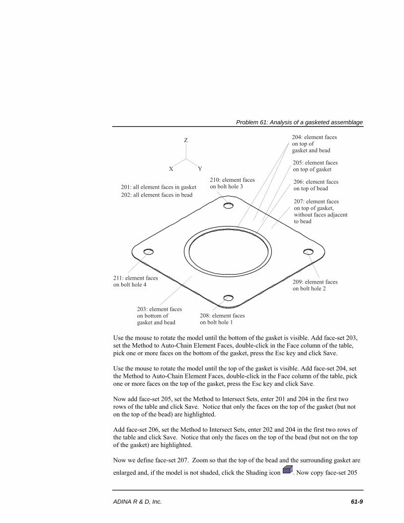
201: all element faces in gasket

202: all element faces in bead

203: element faceson bottom ofgasket and bead

204: element faceson top ofgasket and bead

205: element faceson top of gasket

206: element faceson top of bead

207: element faceson top of gasket,without faces adjacentto bead





X Y

Z

Use the mouse to rotate the model until the bottom of the gasket is visible. Add face-set 203, set the Method to Auto-Chain Element Faces, double-click in the Face column of the table, pick one or more faces on the bottom of the gasket, press the Esc key and click Save. Use the mouse to rotate the model until the top of the gasket is visible. Add face-set 204, set the Method to Auto-Chain Element Faces, double-click in the Face column of the table, pick one or more faces on the top of the gasket, press the Esc key and click Save. Now add face-set 205, set the Method to Intersect Sets, enter 201 and 204 in the first two rows of the table and click Save. Notice that only the faces on the top of the gasket (but not on the top of the bead) are highlighted. Add face-set 206, set the Method to Intersect Sets, enter 202 and 204 in the first two rows of the table and click Save. Notice that only the faces on the top of the bead (but not on the top of the gasket) are highlighted. Now we define face-set 207. Zoom so that the top of the bead and the surrounding gasket are

enlarged and, if the model is not shaded, click the Shading icon . Now copy face-set 205


61-10 ADINA Primer

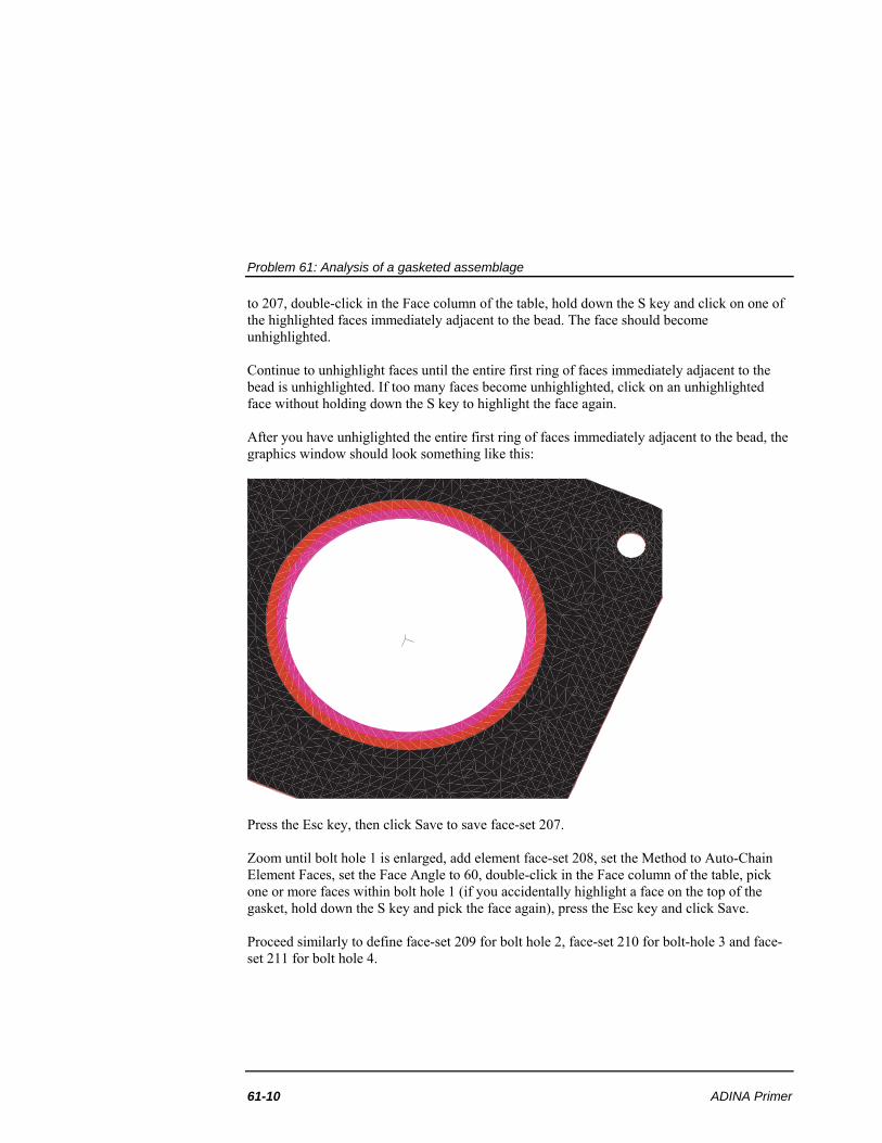
to 207, double-click in the Face column of the table, hold down the S key and click on one of the highlighted faces immediately adjacent to the bead. The face should become unhighlighted. Continue to unhighlight faces until the entire first ring of faces immediately adjacent to the bead is unhighlighted. If too many faces become unhighlighted, click on an unhighlighted face without holding down the S key to highlight the face again. After you have unhiglighted the entire first ring of faces immediately adjacent to the bead, the graphics window should look something like this:

Press the Esc key, then click Save to save face-set 207. Zoom until bolt hole 1 is enlarged, add element face-set 208, set the Method to Auto-Chain Element Faces, set the Face Angle to 60, double-click in the Face column of the table, pick one or more faces within bolt hole 1 (if you accidentally highlight a face on the top of the gasket, hold down the S key and pick the face again), press the Esc key and click Save. Proceed similarly to define face-set 209 for bolt hole 2, face-set 210 for bolt-hole 3 and face-set 211 for bolt hole 4.



Face-sets on cover Now we will define face-sets on the cover:

X Y

Z



402: element faceson top of cover plate

407: element facesinside side of cover cap

409: element facesinside cover cap

408: element facesinside top of cover cap

401: element faceson bottom of cover plate



Using the Model Tree, display zone EG401, and use the mouse to rotate the model until the bottom of the cover is visible. Choose EditPreferences, set Prompt for Label to Yes and click OK. If you closed the Define Element Face Set dialog box, click the Element Face Set

icon . Add element face-set 401, set the Method to Auto-Chain Element Faces, double-click in the Face column of the table, pick one or more faces on the bottom of the cover, press the Esc key and click Save. Choose EditPreferences, set Prompt for Label to NO and click OK. Now use the mouse to rotate the model until the top of the cover is visible, add face-set 402, set the Method to Auto-Chain Element Faces, double-click in the Face column of the table, pick one or more faces on the top of the cover plate, press the Esc key and click Save. Now zoom until bolt hole 1 is enlarged, add element face-set 403, set the Method to Auto-Chain Element Faces, set the Face Angle to 60, double-click in the Face column of the table, pick one or more faces within bolt hole 1, press the Esc key and click Save.


61-12 ADINA Primer

Proceed similarly to define face-set 404 for bolt hole 2, face-set 405 for bolt-hole 3 and face-set 406 for bolt hole 4. Now use the mouse to rotate the model until the underside of the cover cap is visible, add face-set 407, set the Method to Auto-Chain Element Faces, double-click in the Face column of the table, pick one or more faces on the side of the cover cap, press the Esc key and click Save. Add face-set 408, set the Method to Auto-Chain Element Faces, double-click in the Face column of the table, pick one or more faces on the top of the cover cap, press the Esc key and click Save. Now add face-set 409, set the Method to Merge Sets, set the first two rows of the table to 407, 408 and click Save. The graphics window should look something like this:

TIME 1.000

X

Y

Z

You can now close the Define Element Face Set dialog box. Face-sets on bolts: Now we will define face-sets on the bolts, as shown in the figure on the next page. Since we have already demonstrated auto-chaining, we have put the commands necessary to define the face-sets into the file prob61_1.in. Choose FileOpen Batch, navigate to the working directory or folder, select the file prob61_1.in and click Open.



801 for bolt 1, 804 for bolt 2807 for bolt 3, 810 for bolt 4



Now use the Model Tree to display element group 801, unhighlight the group if necessary (for

example, by clicking the Query icon , then clicking on the background of the graphics

window), click the Element Face Set icon and select Face Set 801. The graphics window should look something like this:

TIME 1.000

X Y

Z

You can confirm the definitions of the other face sets by displaying them on the bolt elements. Click OK or Cancel to close the Define Element Face Set dialog box.


61-14 ADINA Primer

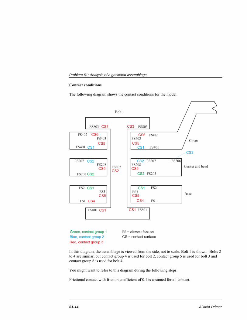
Contact conditions The following diagram shows the contact conditions for the model.

FS1

FS3

FS208

FS403

FS803 FS803

FS802

FS801 FS801

FS403

FS208

FS3FS2 CS1 CS1

CS5 CS5

CS5 CS5

CS5 CS5

CS4 CS4

CS6 CS6

CS1 CS1

CS = contact surface

CS2

CS3 CS3

Green, contact group 1

Blue, contact group 2

Red, contact group 3

CS1 CS1

CS2 CS2

CS2 CS2

CS3

FS203

FS207

FS401

FS402

FS = element face-set

FS207

FS401

FS402

FS206

FS203

FS2

FS1

Base

Gasket and bead

Bolt 1

Cover

In this diagram, the assemblage is viewed from the side, not to scale. Bolt 1 is shown. Bolts 2 to 4 are similar, but contact group 4 is used for bolt 2, contact group 5 is used for bolt 3 and contact group 6 is used for bolt 4. You might want to refer to this diagram during the following steps. Frictional contact with friction coefficient of 0.1 is assumed for all contact.



Contact group 1

Click the Contact Groups icon , add group 1, set the Type to 3-D Contact, and click OK. Choose ModelContactContact Surface (Element Set), add contact surface 1, enter 2 in the first row and column of the table and click Save. Then add contact surface 2, enter 203 in the first row and column of the table and click OK. Now click the Define Contact Pairs icon

, add contact pair 1, set the Target Surface to 1, the Contactor Surface to 2, set the Coulomb Friction Coefficient to 0.1 and click OK. Use the Model Tree to display zone CG1.

When you click the Color Element Groups icon twice, the graphics window should look something like this:

TIME 1.000

X Y

Z

Contact group 2

Click the Contact Groups icon , add group 2, set the Type to 3-D Contact if necessary, and click OK. Choose ModelContactContact Surface (Element Set), define the following contact surfaces and click OK. Contact surface number Element face-set (entered into the

first row and column of the table) 1 401 2 207 3 206


61-16 ADINA Primer

Now click the Define Contact Pairs icon , define the following contact pairs and click OK. Contact pair

number Target

Surface Contactor

Surface Coulomb Friction

Coefficient 1 1 2 0.1 2 1 3 0.1

Finally we define a contact surface offset for surface 3 (= element face-set 206, corresponding to the top surface of the bead). Choose ModelContactContact Surface Offset, enter 3, 0.05 in the first row of the table and click OK. Use the Model Tree to display zone CG2. When you click the Color Element Groups icon

twice, the graphics window should look something like this:

TIME 1.000

X Y

Z

Now use the Model Tree to display zones CG2_CS2, CG2_CS3, EG203 and EG204 simultaneously. When you zoom into the graphics window, the graphics window should look something like the figure at the top of the next page.



No contact segmentsalong this ring of elements Notice that contact surface 2 and contact surface 3 are separated by one ring of elements. In this way all nodes on the top of the gasket and bead are attached to contact surfaces, and contact surfaces 2 and 3 do not share nodes. This is the reason why we defined element face-sets 206 and 207 above. (If we had defined contact surface 2 as element face-set 205, then the ring of nodes on the interface between the gasket and bead would belong to both contact surfaces 2 and 3. This situation would then cause convergence difficulties during the analysis.)


61-18 ADINA Primer

Contact group 3

Click the Contact Groups icon , add group 3, set the Type to 3-D Contact if necessary, set the Compliance Factor to 0.001, uncheck the "Use Continuous Contact-Segment Normal" field and click OK. Choose ModelContactContact Surface (Element Set), define the following contact surfaces and click OK. Contact surface

number Element face-set (entered into the first row and column of the table unless otherwise specified)

1 801 2 802 3 803 4 1 5 3, 208, 403 (in the first three rows of the table) 6 402

Now click the Define Contact Pairs icon , define the following contact pairs and click OK.

Contact pair number

Target Surface

Contactor Surface

Coulomb Friction Coefficient

1 4 1 0.1 2 5 2 0.1 3 6 3 0.1

Use the Model Tree to display zone CG3. When you click the Color Element Groups icon

twice, the graphics window should look something like the figure at the top of the next page. Contact groups 4 to 6 Since the contact groups for the other bolts are similar, we have put the commands necessary to define the contact groups for the other bolts into the file prob61_2.in. Choose FileOpen Batch, navigate to the working directory or folder, select the file prob61_2.in and click Open. You can confirm the definitions of the other contact groups by plotting their zones using the Model Tree.



TIME 1.000

X Y

Z

Boundary conditions

We will fix the bottom of the base. Click the Apply Fixity icon , set the first row of the table to 1 and click OK. Gasket material definition First choose EditPreferences, set Prompt for Label to Yes and click OK. Click the Manage

Materials icon , click the Gasket button and add material 201. In the Curve table, right-click on one of the cells and choose Define. Add Gasket Loading/Unloading curve 201, define it using the following table and click Save.

Closure Pressure 0 0

0.05 1 0.1 2.5 0.3 3 0.5 4.7 0.7 8


61-20 ADINA Primer

Now add the following additional Gasket Loading/Unloading Curves: Curve 202:

Closure Pressure 0.175 0 0.25 1.5 0.3 3

Curve 203:

Closure Pressure 0.305 0 0.42 2.3 0.5 4.7

Curve 204:

Closure Pressure 0.365 0 0.57 4.1 0.7 8

Click OK to close the Define Gasket Loading/Unloading Curves dialog box. In the Define Gasket Material dialog box, set the Density to 2E-9, the Yield Curve to 201, the Yield Point Number on Curve to 3, the Transverse Shear Modulus to 10, the Tensile Young's Modulus to 20, the In-Plane Young's Modulus to 20 and the Poisson's Ratio to 0.3. Then enter 202, 203, 204 in the first three rows of the Loading/Unloading Curves table and click Save. Click the Graph button. The graphics window should look something like the figure at the top of the next page. Click OK, then Close, to close both dialog boxes. Choose EditPreferences, set Prompt for Label to NO and click OK.

Now click the Element Groups icon , choose Group Number 203 and set the Default Material to 201 if necessary, then click Save. Choose Group Number 204 and set the Default Material to 201, then click OK.



0.0 0.1 0.2 0.3 0.4 0.5 0.6 0.70.

1.

2.

3.

4.

5.

6.

7.

8.Pressure-closure curvesfrom material property data

Material 201,gasket

Closure strain

Pre

ssure

We would like to save all results for the gasket element groups. Choose ControlPorthole (.por)Select Element Results, add Result Selection 1, set the Element Group to 203, set Strain to All, set Inelastic to All, set Miscellaneous to All and click Save. Now add Result Selection 2, set the Element Group to 204, set Strain to All, set Inelastic to All, set Miscellaneous to All and click OK. Bolt definitions We need to specify that element groups 801 to 804 are bolt element groups. Click the

Element Groups icon , choose Group Number 801, set the Element Option to Bolt, set the Bolt # to 1, set the Bolt Load to 1.0 and click Save. Repeat for groups 802, 803, 804, setting the Bolt # to 2, 3, 4 respectively (and settting the bolt load to 1.0 for these groups), then click OK.


61-22 ADINA Primer

Choose ModelBoltBolt Options, set the Bolt Loading Sequence Table to Yes and click the Bolt Table ... button. In the Bolt Loading Sequence Table dialog box, add Table 1, set “Bolt Load Interpreted As” to Bolt Shortening, enter the following information into the table and click Save (do not close the Bolt Loading Sequence Table dialog box yet).

Seq. # Bolt # Load Factor Save Results 1 1 3.96 Yes 1 2 3.96 Yes 1 3 3.96 Yes 1 4 3.96 Yes

Now add Table 2, set the Time to 1.0, make sure that “Bolt Load Interpreted As” is set to Tensioning Force, enter the following information into the table and click OK twice to close both dialog boxes.

Seq. # Bolt # Load Factor Save Results 1 1 5000 Yes 2 3 5000 Yes 3 2 5000 Yes 4 4 5000 Yes 5 1 10000 Yes 6 3 10000 Yes 7 2 10000 Yes 8 4 10000 Yes

(Note that bolt 3 is tightened in sequence # 2 and that bolt 2 is tightened in sequence # 3.) Choose ControlTime Step, edit the table as follows and click OK.

Number of Steps

Magnitude

1 1

1.0 8.0

The bolt shortening starts at time 0.0 and has a duration of 1 second. The program then performs a solution step with time step size 1 second. Then the bolt tensioning starts at time 1.0 and has a duration of 8 seconds. Since there are eight bolt sequences, each bolt sequence has a duration of 1 second. The program then performs a solution step with time step size 8 seconds.



Control parameters, including low-speed dynamics Choose ControlHeading, set the Problem Heading to 'Problem 61: Analysis of a gasketed assemblage' and click OK. Choose ControlSolution Process, click the Method button, set the Maximum Number of Iterations to 999 and click OK to close the Nonlinear Iteration Settings dialog box. Now click the Tolerances button, set the Convergence Criteria to Energy and Force, set the Reference Force to 1.0, the Reference Moment to 1.0, the Contact Force Tolerance to 0.01, and the Maximum Incremental Displacement in Any Iteration to 1.0. Click OK twice to close both dialog boxes.

Click the Analysis Options icon and click the ... button to the right of the ‘Use Automatic Time Stepping (ATS)’ field. Set 'Use Low-Speed Dynamics' to 'On Element Groups' and click the ... button to the right of that field. In the Define Rayleigh Damping Factors dialog box, set the default Alpha (Mass) to 1.0, then click OK to close the Define Rayleigh Damping Factors dialog box. In the Automatic Time-Stepping (ATS) dialog box, set 'Maximum Subdivisions Allowed' to 1000, 'Max. Factor for Accelerating Time Step' to 1.0, 'Time Integration Method' to Newmark, 'Low-Speed Dynamics Inertia Factor' to 0, then click OK twice to close both dialog boxes. Generating the ADINA Structures data file, running ADINA Structures, loading the porthole file

First click the Save icon and save the database to file prob61. Click the Data

File/Solution icon , set the file name to prob61a, make sure that the Run Solution button is checked and click Save. In the ADINA Structures dialog box, in the Message window, notice the lines Bolt iterations: step number = 1 bolt force factor = 3.9600000E+00 ... Starting time step calculations... Step number = 1 step size = 1.0000000E+00 time = 1.0000000E+00 Porthole file updated, nodal results saved Porthole file updated, element results saved Restart file created Bolt iterations: step number = 1 bolt force factor = 5.0000000E+03 Porthole file updated, nodal results saved Porthole file updated, element results saved Bolt iterations: step number = 2 bolt force factor = 5.0000000E+03 Porthole file updated, nodal results saved Porthole file updated, element results saved Bolt iterations: step number = 3 bolt force factor = 5.0000000E+03 Porthole file updated, nodal results saved Porthole file updated, element results saved Bolt iterations: step number = 4 bolt force factor = 5.0000000E+03


61-24 ADINA Primer

Porthole file updated, nodal results saved Porthole file updated, element results saved Bolt iterations: step number = 5 bolt force factor = 1.0000000E+04 Porthole file updated, nodal results saved Porthole file updated, element results saved Bolt iterations: step number = 6 bolt force factor = 1.0000000E+04 Porthole file updated, nodal results saved Porthole file updated, element results saved Bolt iterations: step number = 7 bolt force factor = 1.0000000E+04 Porthole file updated, nodal results saved Porthole file updated, element results saved Bolt iterations: step number = 8 bolt force factor = 1.0000000E+04 Step number = 2 step size = 8.0000000E+00 time = 9.0000000E+00 Porthole file updated, nodal results saved Porthole file updated, element results saved Restart file created

We see that ADINA Structures performs a bolt step, then a solution step. This corresponds to the first bolt table (length shrinking). Then ADINA Structures performs 8 bolt steps and another solution step, and this corresponds to the second bolt table (force tensioning). Close all open dialog boxes, set the Program Module drop-down list to Post-Processing (you

can discard all changes), click the Open icon and open porthole file prob61a. Post-processing for the initial assembly and bolt tensioning analysis

Contact on gasket: Click the Color Element Groups icon , then use the Model Tree to

display element groups 203 and 204. Click the Create Band Plot icon , set the Band Plot Variable to (Contact: NODAL_CONTACT_STATUS), then click OK . The graphics window should look something like the figure at the top of the next page. The entire gasket is in sticking contact.

Now click the First Solution icon to observe the state of contact after the bolts are shortened, but before the bolts are tensioned. For solution time 1, contact is established on the

bead, and also on the edge of the gasket. Click the Next Solution icon repeatedly to observe how contact develops as the bolts are tensioned. The gasket is in contact at the end of bolt sequence 4 (5000 N in all bolts), and remains in contact thereafter. Click the Last

Solution icon to display the last solution.

Gasket pressure: Now click the Clear Band Plot icon , then click the Create Band Plot

icon , set the Band Plot Variable to (Stress: GASKET_PRESSURE), then click OK . The graphics window should look something like the figure at the bottom of the next page.



TIME 9.000

X Y

Z

NODALCONTACTSTATUS

TIME 9.000

STICKINGSLIPPINGCLOSEDOPENDEAD

MAXIMUMSTICKING

NODE 4340

MINIMUMSTICKING

NODE 4340

TIME 9.000

X Y

ZGASKET_PRESSURE

RST CALC

TIME 9.000

2.667

2.400

2.133

1.867

1.600

1.333

1.067

MAXIMUM2.777

EG 203, EL 2093, IPT 212 (2.769)

MINIMUM0.9165

EG 203, EL 2468, IPT 112 (1.227)


61-26 ADINA Primer

The largest pressures are on the bead and on the four corners of the gasket. Click the First

Solution icon then click the Next Solution icon repeatedly to observe how the gasket pressure changes as the bolts are tensioned. The gasket pressures underneath the bolts increase, as expected. The entire gasket is under pressure at bolt tension of 5000 N, and this

pressure increases at bolt tension 10000 N. Click the Last Solution icon to display the last solution. Bolt forces: Choose ListValue ListZone, set Variable 1 to (Displacement: BOLT-DISPLACEMENT), Variable 2 to (Force: BOLT-FORCE) and click Apply. Observe that the bolt displacements for time 0.0, bolt sequence 1 are 3.96000E+00 (mm), the bolt forces for time 0.0, bolt sequence 1 are approximately 5.6E+01 (N) and the bolt forces for time 1.0 are nearly the same as for bolt sequence 1. For time 1.0, bolt sequence 1, the bolt displacement for bolt 1 is 4.15678E+00 and the bolt force is 5.00000E+03 (equal to the specified bolt force). For time 1.0, bolt sequence 2, the bolt displacement for bolt 1 is unchanged, but the bolt force changes to 5.34709E+03. For each of the bolt sequences in time 1, the bolt that is being tensioned has the specified bolt force (with a changed bolt displacement) , and the remaining bolts have unchanged bolt displacements and changed bolt forces. The solution for time 9.0 is slightly different than the solution for time 1.0, bolt sequence 8, due to the use of low-speed dynamics. But this change in solution is small. Model definition for the pressure application analysis Set the Program Module drop-down list to ADINA Structures (you can discard all changes) and choose database file prob61.idb from the recent file list near the bottom of the File menu. Restart analysis, turning off low-speed dynamics Choose ControlSolution Process, set the Analysis Mode to Restart Run, set the Solution Start Time to 9 and click OK.

Click the Analysis Options icon and click the ... button to the right of the 'Use Automatic Time Stepping (ATS)' field. Set 'Use Low-Speed Dynamics' to No and click OK twice to close both dialog boxes.



Pressure loading

Click the Apply Load icon , set the Load Type to Pressure and click the Define... button to the right of the Load Number field. In the Define Pressure dialog box, add pressure 1, set the Magnitude to 1 and click OK. In the Apply Load dialog box, make sure that the “Apply to” field is set to Element-Face Set and, in the first two rows of the table, set the Set # to 7 and 409. Click OK to close the Apply Load dialog box. Choose ControlTime Step, edit the table as follows and click OK.

Number of Steps

Magnitude

10 0.1 Choose ControlTime Function, edit the table as follows and click OK.

Time Value 0 9

0 0

10 4 The pressure loading starts at time 9.0, for 1 second. The pressure load is applied as a ramp in 10 equal steps of 0.1 seconds.

Now click the Clear icon , the Mesh Plot icon and the Load Plot icon . Use the mouse to rotate the model until the graphics window looks something like the figure at the top of the next page.


61-28 ADINA Primer

TIME 10.00

X YZ

PRESCRIBED

PRESSURE

TIME 10.00

4.000

Generating the ADINA Structures data file, running ADINA Structures, loading the porthole file

First click the Save icon to save the database to file prob61. Click the Data File/Solution

icon , set the file name to prob61b, make sure that the Run Solution button is checked and click Save. The AUI opens a window in which you specify the restart file from the first analysis. Enter restart file prob61a and click Copy. When ADINA Structures is finished, close all open dialog boxes, set the Program Module

drop-down list to Post-Processing (you can discard all changes), click the Open icon and open porthole file prob61b. Post-processing for the pressure application analysis

Contact on gasket: Click the Color Element Groups icon , then use the Model Tree to

display element groups 203 and 204. Click the Create Band Plot icon , set the Band Plot Variable to (Contact: NODAL_CONTACT_STATUS), then click OK. The graphics window should look something like the figure on the next page.



TIME 10.00

X Y

Z

NODALCONTACTSTATUS

TIME 10.00

STICKINGSLIPPINGCLOSEDOPENDEAD

MAXIMUMSTICKING

NODE 4340

MINIMUMOPEN

NODE 4825

Most of the gasket is in contact, but the area near the bead is beginning to open.

Click the First Solution icon , then click the Next Solution icon repeatedly to observe the contact status as the pressure is applied. As the pressure is applied, slipping begins to

occur and the area near the bead starts to open. Click the Last Solution icon to display the last solution.

Gasket pressure: Now click the Clear Band Plot icon , then click the Create Band Plot

icon , set the Band Plot Variable to (Stress: GASKET_PRESSURE), then click OK . The graphics window should look something like the figure on the next page.


61-30 ADINA Primer

TIME 10.00

X Y

Z

GASKET_PRESSURE

RST CALC

TIME 10.00

2.700

2.250

1.800

1.350

0.900

0.450

0.000

MAXIMUM2.860

EG 203, EL 2099, IPT 121 (2.850)

MINIMUM-0.1667

EG 203, EL 1952, IPT 111 (0.01209)

Use the First Solution icon and Next Solution icon to observe the gasket pressures during pressure application. As the pressure is applied, the gasket pressure decreases. Click

the Last Solution icon to display the last solution.

Gasket plastic strain: Now click the Clear Band Plot icon , then click the Create Band

Plot icon , set the Band Plot Variable to (Strain: GASKET_PLASTIC_CLOSURE_ STRAIN), then click OK . The graphics window should look something like the figure on the next page.



TIME 10.00

X Y

Z

GASKETPLASTICCLOSURESTRAIN

RST CALC

TIME 10.00

0.1170

0.0990

0.0810

0.0630

0.0450

0.0270

0.0090

MAXIMUM0.1259

EG 203, EL 2099, IPT 121 (0.1226)

MINIMUM-0.002481

EG 203, EL 2711, IPT 212 (0.0004232)

Again, by examining all of the solution steps, we can observe that the gasket has already become plastic at the bolt tension 10000 N, and the plasticity is unchanged during the

pressure application. Click the Last Solution icon to display the last solution. Gasket pressure minus applied pressure When the gasket pressure in the bead is greater than the applied pressure, we anticipate that the gasket will not leak, but when the gasket pressure is less than the applied pressure, we anticipate that the gasket will leak. So we will plot the gasket pressure minus the applied pressure on the bead, to observe if this quantity ever becomes negative.

Click the Clear icon , then use the Model Tree to display element group 204. Choose DefinitionsVariableResultant, add resultant GASKET_PRESS_MINUS_APP_PRESS, define the resultant as GASKET_PRESSURE - TIME_FUNCTION_1

and click OK. Now click the Create Band Plot icon , set the Band Plot Variable to <User Defined: GASKET_PRESS_MINUS_APP_PRESS>, then click OK. The graphics window should look something like the figure at the top of the next page.


61-32 ADINA Primer

TIME 10.00

X Y

Z

GASKETPRESSMINUSAPPPRESS

RST CALC

TIME 10.00

-3.390

-3.420

-3.450

-3.480

-3.510

-3.540

-3.570

MAXIMUM-3.372

EG 204, EL 2989, IPT 121 (-3.390)

MINIMUM-3.592

EG 204, EL 3000, IPT 122 (-3.584)

Since this variable is negative, we see that the gasket is leaking at the applied pressure of 4 MPa.

Now click the First Solution icon . The band plot scaling is not adjusted, so we cannot see the results. To rescale the band plot when the solution time is changed, click the Modify Band

Plot icon , click the Band Table... button, then, in the Value Range box, set the Maximum and Minimum to Automatic and uncheck the Freeze Range field. Click OK to close both dialog boxes. The graphics window should look something like the figure at the top of the next page.

Now, each time you click the Next Solution icon , the band plot scaling changes. Observe that, at time 9.4, the minimum value of the variable becomes negative, hence the gasket will leak at that solution time. Since the applied pressure at time 9.4 is 0.4 4 1.6 MPa , the

gasket will leak at this applied pressure. Exiting the AUI: Choose FileExit to exit the AUI. You can discard all changes.



TIME 9.100

X Y

Z

GASKETPRESSMINUSAPPPRESS

RST CALC

TIME 9.100

1.920

1.893

1.867

1.840

1.813

1.787

1.760

MAXIMUM1.936

EG 204, EL 2983, IPT 211 (1.910)

MINIMUM1.749

EG 204, EL 3000, IPT 122 (1.754)

Modeling comments 1) The .nas file used in this run is created using ADINA-M/PS. You can examine the commented-out lines in file prob61.in in order to see the commands used for creating the mesh and exporting the Nastran file. 2) Incompatible modes elements are used in element groups 2 and 401, since these groups might undergo significant bending. 3) In the Nastran file, the components are defined with gaps between them, as shown in the figure:

Base

Gasket and bead

(not drawn to scale)

Cover1 mm

1 mm 0.05 mm

1 mm

1 mm


61-34 ADINA Primer

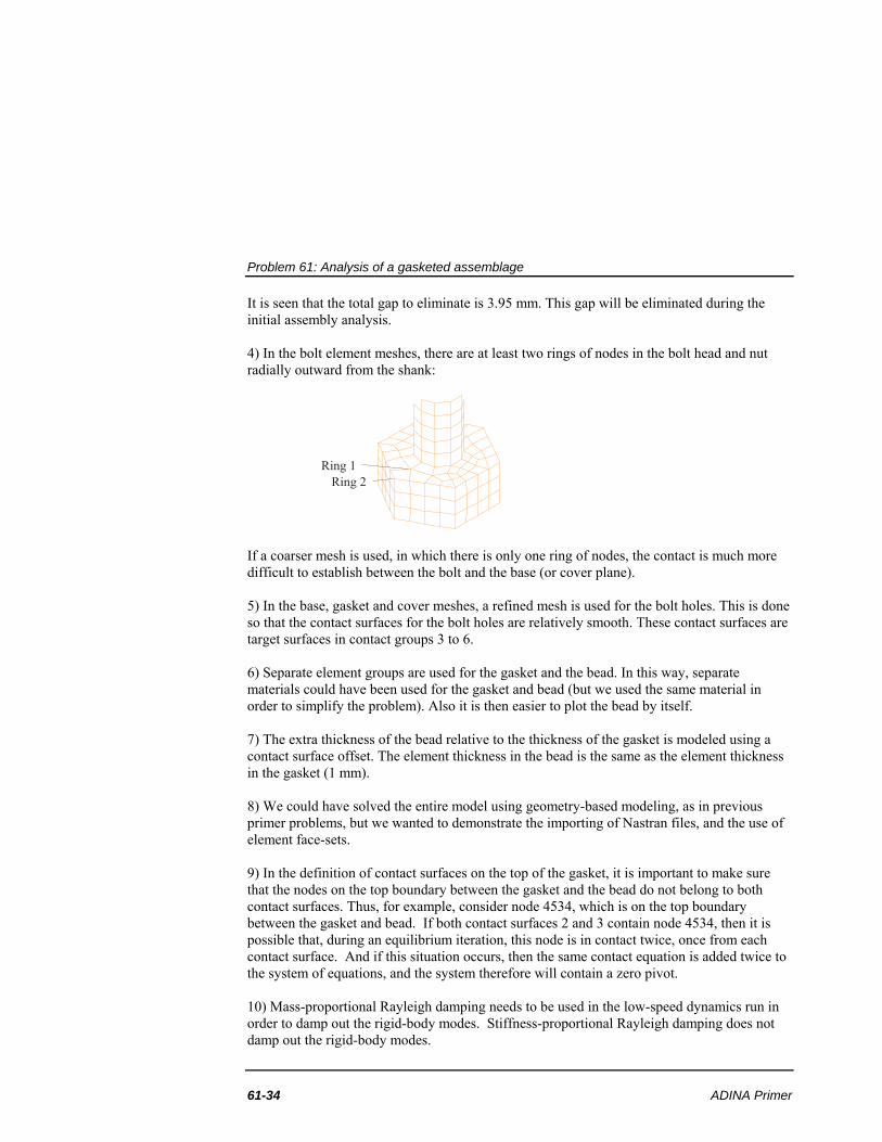
It is seen that the total gap to eliminate is 3.95 mm. This gap will be eliminated during the initial assembly analysis. 4) In the bolt element meshes, there are at least two rings of nodes in the bolt head and nut radially outward from the shank:

Ring 1

Ring 2

If a coarser mesh is used, in which there is only one ring of nodes, the contact is much more difficult to establish between the bolt and the base (or cover plane). 5) In the base, gasket and cover meshes, a refined mesh is used for the bolt holes. This is done so that the contact surfaces for the bolt holes are relatively smooth. These contact surfaces are target surfaces in contact groups 3 to 6. 6) Separate element groups are used for the gasket and the bead. In this way, separate materials could have been used for the gasket and bead (but we used the same material in order to simplify the problem). Also it is then easier to plot the bead by itself. 7) The extra thickness of the bead relative to the thickness of the gasket is modeled using a contact surface offset. The element thickness in the bead is the same as the element thickness in the gasket (1 mm). 8) We could have solved the entire model using geometry-based modeling, as in previous primer problems, but we wanted to demonstrate the importing of Nastran files, and the use of element face-sets. 9) In the definition of contact surfaces on the top of the gasket, it is important to make sure that the nodes on the top boundary between the gasket and the bead do not belong to both contact surfaces. Thus, for example, consider node 4534, which is on the top boundary between the gasket and bead. If both contact surfaces 2 and 3 contain node 4534, then it is possible that, during an equilibrium iteration, this node is in contact twice, once from each contact surface. And if this situation occurs, then the same contact equation is added twice to the system of equations, and the system therefore will contain a zero pivot. 10) Mass-proportional Rayleigh damping needs to be used in the low-speed dynamics run in order to damp out the rigid-body modes. Stiffness-proportional Rayleigh damping does not damp out the rigid-body modes.



11) The bolt length reduction needs to be at least 3.95 mm, in order to eliminate the gap. If 3.95 mm were used, then only the bead would be in contact at the end of the initial assembly. However we use 3.96 mm, so that the bead and also the edges of the gasket are in contact at the end of the initial assembly. 12) Because many nodes are coming into contact, many equilibrium iterations need to be used in each bolt sequence step in order to obtain convergence. Once the bolts are tensioned so that the entire gasket is in contact, then only a few equilibrium iterations are required in each step thereafter. 13) Low-speed dynamics is used during bolt tensioning because the bolts can go out-of-contact in the trial (non-converged) solutions during the equilibrium iterations.


61-36 ADINA Primer

This page intentionally left blank.

problem 61: analysis of a gasketed assemblage - … · problem 61: analysis of a gasketed...

Documents