problem solving: informed search - dieearmano/ia-bilingue/2005/slides/2.2 - heuristic... · problem...

Problem Solving: Informed Search

References● Russell and Norvig, Artificial Intelligence: A modern approach, 2nd ed.

Prentice Hall, 2003 (Chapters 1,2, and 4)● Nilsson, Artificial intelligence: A New synthesis. McGraw Hill, 2001

OutlineBest first search - Greedy search - A* search - Dijkstra's algorithmMore on best first search - Dominance - Relaxed problemsIterative improvement - Hill climbing - Simulated annealing

Informed (heuristic) Search

search

non-adversary

adversary

informed

uninformed

or “blind”

or “heuristic”

Informed (heuristic) SearchInformed search strategies, other than the

information available in the problem definition, use other information, such as heuristics to guide search towards a good solution

heuristic search

Heuristic search: Best first searchBest first search - Greedy search - A* search - Dijkstra's algorithmMore on best first search - Dominance - Relaxed problemsIterative improvement - Hill climbing - Simulated annealing

heuristic search: best first search

Recall the general tree search algorithmdefun TREE-SEARCH (problem, fringe) returns solution state ← INITIAL-STATE(problem) fringe.insert(MAKE-NODE(state)) loop do if EMPTY?(fringe) then return *FAILURE* node ← fringe.remove() if problem.GOAL-TEST?(STATE(node)) then return SOLUTION(node) children ← problem.EXPAND(node) for each node in children do fringe.insert(node)

The search strategy is defined by the order of node expansion !


Recall the general tree search algorithmdefun EXPAND(problem, node) returns successors successors ← {} --- set of NODES, initially empty for each action, state in problem.SUCCESSORS(STATE(node)) do child ← new NODE, child.parent ← node child.action ← action, child.state ← state step-cost ← problem.STEP-COST(STATE(node), action, state) child.cost ← COST(node) + step-cost child.depth ← DEPTH(node) + 1 successors.add(child) return successors


Best-first searchIdea:

For each node use an evaluation function, able to estimate the “goodness” of the node

The “goodness” of a node says how promising is the node towards the solution

Expand the “best” unexpanded node

Implementation: fringe is a queue sorted in decreasing order of “goodness”

Special cases:Greedy searchA* search


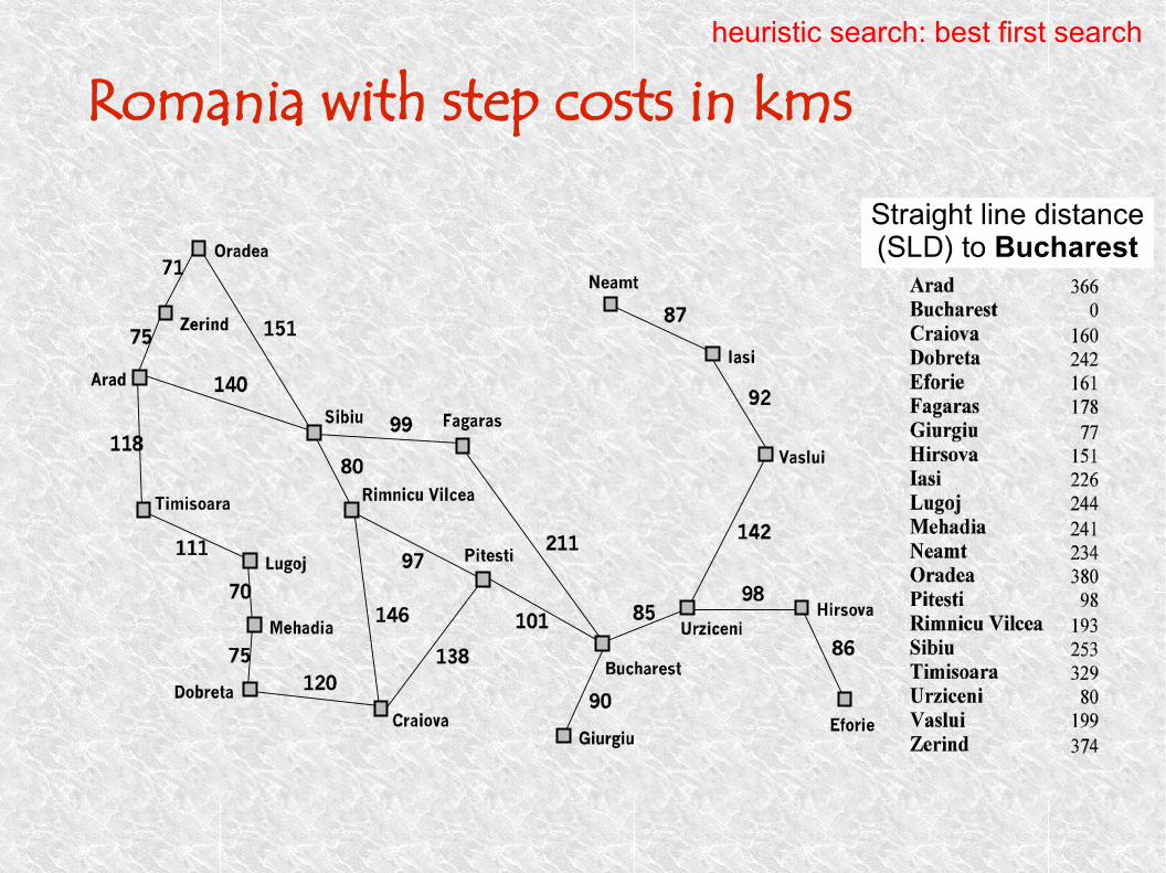
Romania with step costs in kms

Straight line distance (SLD) to Bucharest


Best first search: Greedy searchBest first search - Greedy search - A* search - Dijkstra's algorithmMore on best first search - Dominance - Relaxed problemsIterative improvement - Hill climbing - Simulated annealing

heuristic search: best first search: greedy search

Greedy searchIdea: greedy search expands the node that

appears to be closest to the goalEvaluation function f(n) = h(n)

The cost for attaining the current node is not taken into account

Only an estimation about how “far” (in terms of cost) is the node from the goal is considered (e.g. hSLD(n) = straight-line distance from the current node n to Bucharest)


Greedy searchImplementation: The intended behavior can be

ensured by using an ordered queue in which nodes are inserted according to the value returned by the function f(n) = h(n)

defun GREEDY-SEARCH(problem) returns solution return TREE-SEARCH ( problem, ordered-queue )


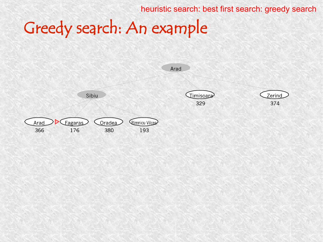
Greedy search: An exampleheuristic search: best first search: greedy search

Greedy searchCompleteness:

NO —it can get stuck in loops, e.g. if Oradea is a goal, loop Lasi → Neamt → Lasi → Neamt

It is complete only under the assumption that state space is finite and that we check for repeated states

Time complexity:O(bm) --- recall that m = max depth of the search spaceA good heuristic can improve it tremendously

Space complexity:O(bm) --- keeps all nodes in memory

Optimality:No


Best first search: A* searchBest first search - Greedy search - A* search - Dijkstra's algorithmMore on best first search - Dominance - Relaxed problemsIterative improvement - Hill climbing - Simulated annealing

heuristic search: best first search: A-star search

A* searchIdea: avoid expanding paths that are already

expensiveEvaluation function f(n) = g(n) + h(n) g(n) actual cost spent so far to reach n (from

the initial state) h(n) estimated cost to reach the goal (from the

current node n)In practice, uniform-cost search and greedy

search are “put together” to give rise to the most powerful algorithm in this category


A* searchA* search uses an admissible heuristic h(n)

In other words, 0 ≤ h(n) ≤ h*(n), where h*(n) is the true cost from n to the goal (e.g. hSLD(n) never overestimates the actual driving distance)

By definition, h(G)=0 for any state G that satisfies the goal


A* searchImplementation: The intended behavior can be

ensured by using an ordered queue in which nodes are inserted according to the function f(x) = g(x) + h(x)

defun A-STAR-SEARCH(problem) returns solution return TREE-SEARCH ( problem, ordered-queue )


A* search: An example heuristic search: best first search: A-star search

A* search: An exampleheuristic search: best first search: A-star search

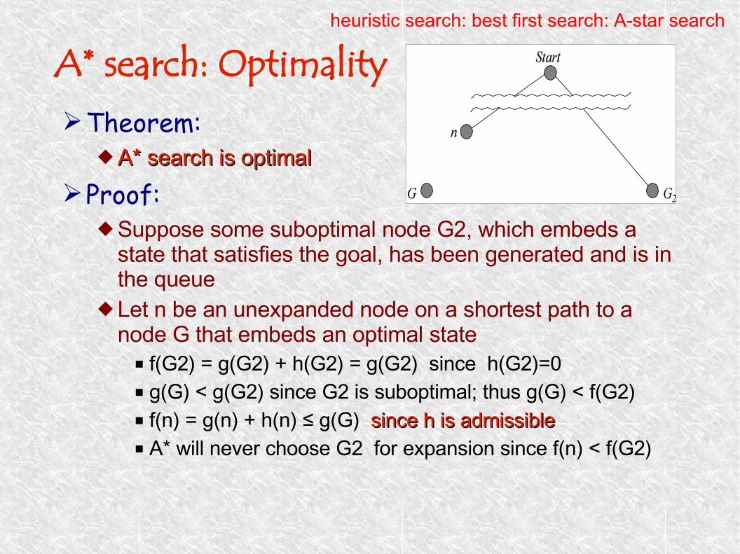
A* search: OptimalityTheorem:

A* search is optimalA* search is optimal

Proof: Suppose some suboptimal node G2, which embeds a

state that satisfies the goal, has been generated and is in the queue

Let n be an unexpanded node on a shortest path to a node G that embeds an optimal state■ f(G2) = g(G2) + h(G2) = g(G2) since h(G2)=0 ■ g(G) < g(G2) since G2 is suboptimal; thus g(G) < f(G2) ■ f(n) = g(n) + h(n) ≤ g(G) since h is admissiblesince h is admissible■ A* will never choose G2 for expansion since f(n) < f(G2)


A* search: Optimality (another way)Lemma: A* expands nodes in increasing order of f value

It gradually adds “f-contours” of nodesContour k contains all nodes with f = fk with fk < fk+1

If C* is an optimal-path cost: ■ A* expands all nodes with f(n) < C*■ A* expands some nodes with f(n) = C*■ A* does not expand nodes with f(n) > C*


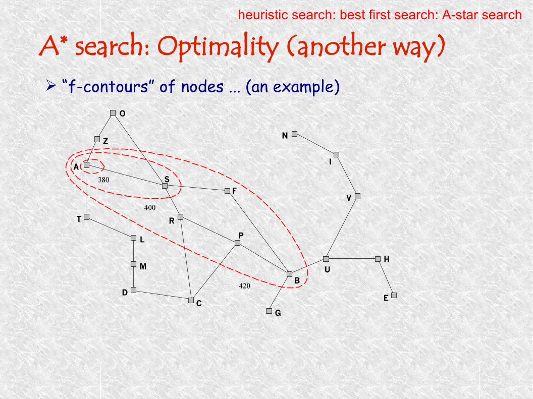
A* search: Optimality (another way) “f-contours” of nodes ... (an example)


Proof of lemma: ConsistencyA heuristic h is consistent if

h(n) ≤ c(n,a,n') + h(n')

If h is consistent, then f(n') ≥ f(n) f(n') = g(n') + h(n') f(n') = g(n) + c(n,a,n') + h(n') ≥ g(n) + h(n) f(n') = g(n) + c(n,a,n') + h(n') ≥ f(n)

Hence, f(n) is non-decreasing along any path (cf. triangle inequality)

Let us assume that the function devised to evaluate the cost of a step (i.e STEP-COST) has a corresponding function c : node x action x node


A* search: PropertiesCompleteness:

Yes, unless there is an infinite number of nodes with f ≤ f(G)

Time complexity:O(bd) --- d = depth of the closest optimal solutionA good heuristic (i.e. h(x) very close to h*(x)) can improve it

very much

Space complexity:O(bd) --- keeps all nodes in memory

Optimality:Yes --- it cannot expand fk+1 until fk is finished


Best first searchBest first search - Greedy search - A* search - Dijkstra's algorithmMore on best first search - Dominance - Relaxed problemsIterative improvement - Hill climbing - Simulated annealing

heuristic search: best first search: Djikstra's algorithm

Dijkstra’a algorithmGiven a vertex v, what is the length of the

shortest path from v to every vertex v' in the graph?

A greedy algorithm: choose node that minimized distance from initial state (i,e, use g instead of h)

You must know the entire search space to use Dijkstra's algorithm


A* vs. Dijkstra's AlgorithmDijkstra’s algorithm is a degenerate case of A*,

where h(n) = 0 - A* finds the best path to a particular v - A* will typically use less memory


A* vs. Dijkstra's AlgorithmDijkstra's is like a puddle of water flooding

outwards on a flat floor, whereas A* is like the same puddle expanding on a bumpy and graded floor toward a drain (the target node) at the lowest point in the floor


A* vs. Dijkstra's AlgorithmInstead of spreading out evenly

on all sides, the water seeks the path of least resistance, only trying new paths when something gets in its way

The heuristic function is what provides the “grade” of the hypothetical floor.


Best first search - Greedy search - A* search - Dijkstra's algorithmMore on best first search - Dominance - Relaxed problemsIterative improvement - Hill climbing - Simulated annealing

More on best first searchheuristic search: best first search: more on ...

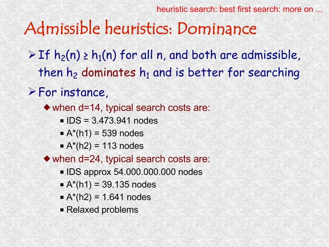
Admissible heuristics: DominanceIf h2(n) ≥ h1(n) for all n, and both are admissible,

then h2 dominates h1 and is better for searchingFor instance,

when d=14, typical search costs are:■ IDS = 3.473.941 nodes ■ A*(h1) = 539 nodes■ A*(h2) = 113 nodes

when d=24, typical search costs are:■ IDS approx 54.000.000.000 nodes■ A*(h1) = 39.135 nodes ■ A*(h2) = 1.641 nodes■ Relaxed problems

heuristic search: best first search: more on ...

Admissible heuristics (8-puzzle)Examples of admissible heuristics for the 8-

puzzle problem:h1(n) = number of misplaced tiles

h2(n) = total Manhattan distance (for all tiles, sum the number of squares from tile location to desired location)


Admissible heuristics: RelaxationBest first search - Greedy search - A* search - Dijkstra's algorithmMore on best first search - Admissible heuristics - Relaxed problemsIterative improvement - Hill climbing - Simulated annealing


Admissible heuristics: RelaxationOne way to obtain admissible heuristics is:

Simplify the problem by relaxing some of its constraintsFind an exact solution for the relaxed problem (easier than

the initial problem)Use the cost of the exact solution for the relaxed problem

as the heuristic value

Key: the optimal solution cost to the relaxed problem cannot be greater than that of the real problem


Relaxed problems: 8-puzzleRelax 8-puzzle rules so that a tile can move to

any squareUnder this hypothesis, h1(n) (number of misplaced tiles)

gives the shortest solution

Relax 8-puzzle rules so that a tile can move to any adjacent square (even if it is full) Under this hypothesis, h2(n) (Manhattan distance) gives

the shortest solution


More relaxed problems (TSP)Traveling Salesman Problem (TSPTSP) = find the

shortest tour that visits all cities exactly once

Relaxation: minimum spanning tree can be computed in O(n2) and it is a lower bound on shortest (open) tour


More relaxed problems (n-Queens) n-Queensn-Queens = place n queens on an n x n board such

that no two queens are placed on the same row, column or diagonal

Strategy: start with any queen distribution on the board. Move a queen at a time to reduce number of conflicting pairs


Iterative improvementBest first search - Greedy search - A* search - Dijkstra's algorithmMore on best first search - Dominance - Relaxed problemsIterative improvement - Hill climbing - Simulated annealing

heuristic search: iterative improvement

Iterative improvementIn many optimization problems the path to the

solution is irrelevant. The goal state itself is the solution (e.g. TSP and n-Queen problems)

All problems in which a configuration or schedule that meets some constraints must be found satisfy this description

In such kind of problems, the state space represents the set of complete configurations and iterative improvementiterative improvement of the solution can be adopted as a strategy to search for a solution


Iterative improvementStrategy:

Keep a single “current” state and try to improve it “Repair” the solution until it meets all constraints

Space complexity:constant


Iterative improvement (TSP)Start with any complete tour. Perform pairwise

exchangesThe sequence of steps does not matter. We want

the goal state (tour)


Iterative improvement (n-Queens)Start with any queen distribution on the boardMove a queen at a time to reduce the number of

conflicting pairs


Iterative improvement: Hill climbingBest first search - Greedy search - A* search - Dijkstra's algorithmMore on best first search - Dominance - Relaxed problemsIterative improvement - Hill climbing - Simulated annealing


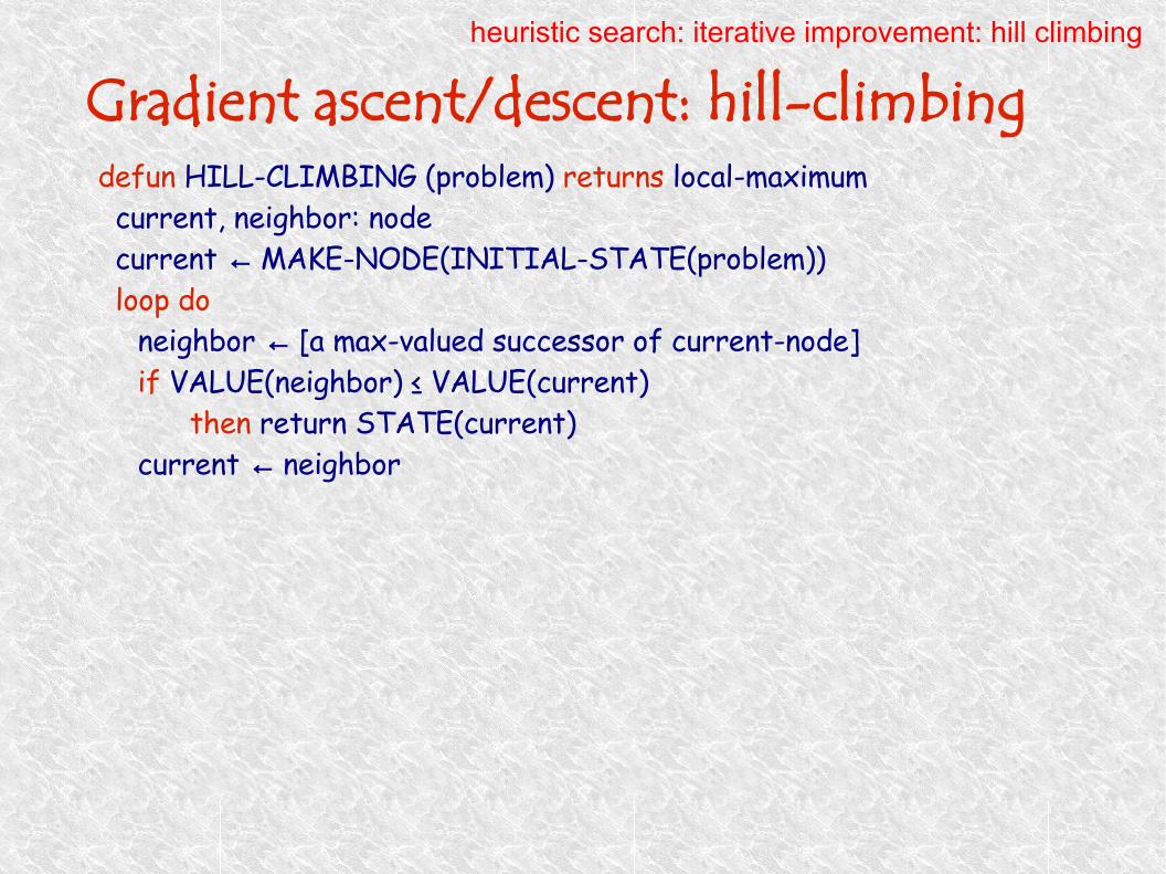
Gradient ascent/descent: hill-climbingdefun HILL-CLIMBING (problem) returns local-maximum current, neighbor: node current ← MAKE-NODE(INITIAL-STATE(problem)) loop do neighbor ← [a max-valued successor of current-node]

if VALUE(neighbor) ≤ VALUE(current) then return STATE(current) current ← neighbor

heuristic search: iterative improvement: hill climbing

Gradient ascent/descent: hill-climbingCan get stuck on local maxima, depending or

initial state

If space is continuous: problems choosing step size, slow convergence

States

Local maximum

Global maximumValue

heuristic search: iterative improvement: hill climbing

Simulated AnnealingBest first search - Greedy search - A* search - Dijkstra's algorithmMore on best first search - Dominance - Relaxed problemsIterative improvement - Hill climbing - Simulated annealing

heuristic search: iterative improvement: simulated annealing

Simulated annealingIdea: escape local maxima allowing some “bad”

moves, but gradually reducing their frequency and size


Simulated annealingSimilar to the annealing process in metalurgics:

drop temperature gradually allows crystalline structure reach a minimal energy state

If T decreases slowly enough, always reaches the best state

Widely used in VLSI design, flight scheduling, production scheduling, and other large optimization problems


Simulated annealingEach point s of the search space is compared to

a state of some physical system, and the function E(s) to be minimized is interpreted as the internal energy of the system in that state

The goal is to bring the system, from an arbitrary initial state, to a state with the minimum energy


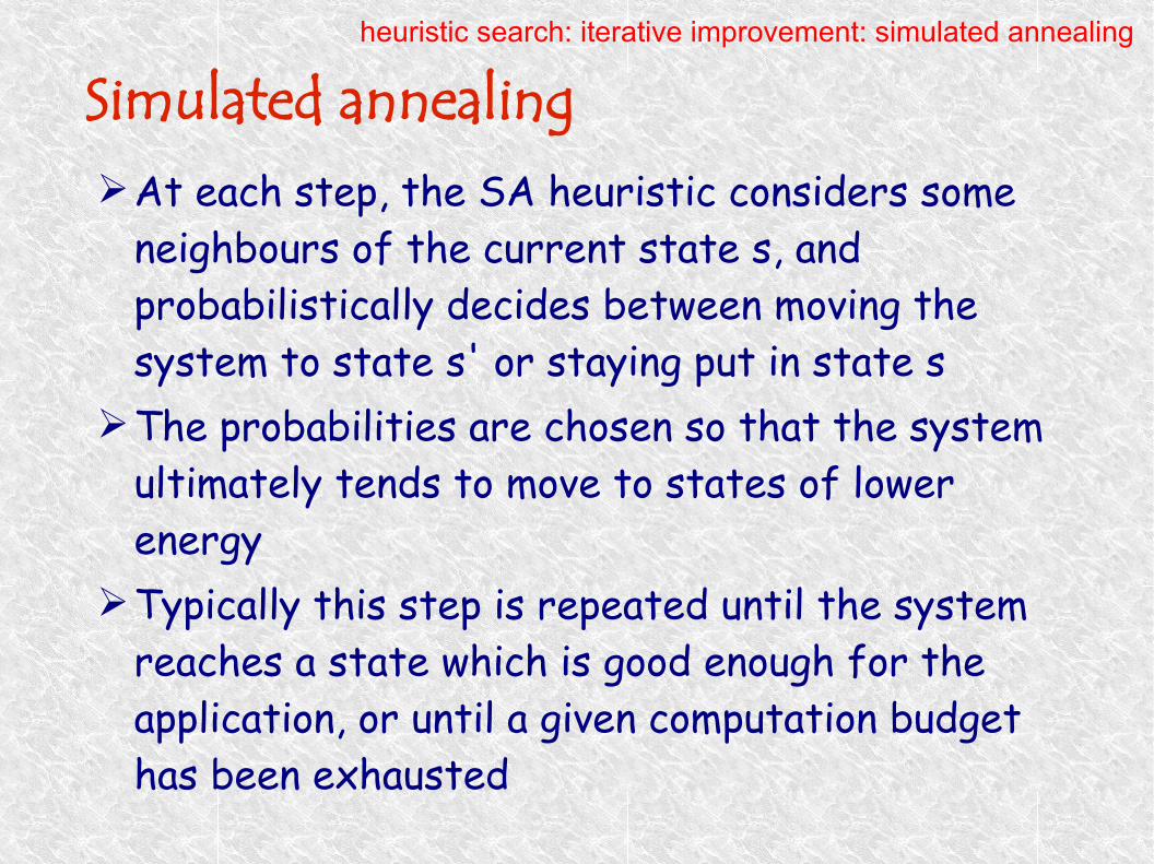
Simulated annealingAt each step, the SA heuristic considers some

neighbours of the current state s, and probabilistically decides between moving the system to state s' or staying put in state s

The probabilities are chosen so that the system ultimately tends to move to states of lower energy

Typically this step is repeated until the system reaches a state which is good enough for the application, or until a given computation budget has been exhausted


Simulated annealingdefun SIM-ANNEALING(problem,schedule) returns goal-state current, next: node, T: Temperature current ← MAKE-NODE ( INITIAL-STATE(problem) ) k ← 1 loop do

T ← schedule[k] if T = 0 then return STATE(current)

next ← [a randomly selected successor of current] ∆ ← EVAL(next) – EVAL(current) if ∆ > 0 then current ← next --- only with probability e∆/T

else current ← next k ← k+1

TemperatureTemperature:controls the probability of downward steps (varies according to schedule)


problem solving: informed search - dieearmano/ia-bilingue/2005/slides/2.2 - heuristic... · problem...

Documents