problems for the course f5170 { introduction to plasma...
TRANSCRIPT
Problems for the Course F5170 –Introduction to Plasma Physics
Jirı Sperka, Jan Vorac, Lenka Zajıckova
Department of Physical ElectronicsFaculty of Science
Masaryk University
2014

Contents
1 Introduction 51.1 Theory . . . . . . . . . . . . . . . . . . . . . . . . . . . . . . . 51.2 Problems . . . . . . . . . . . . . . . . . . . . . . . . . . . . . 6
1.2.1 Derivation of the plasma frequency . . . . . . . . . . . 61.2.2 Plasma frequency and Debye length . . . . . . . . . . 71.2.3 Debye-Huckel potential . . . . . . . . . . . . . . . . . 8
2 Motion of particles in electromagnetic fields 92.1 Theory . . . . . . . . . . . . . . . . . . . . . . . . . . . . . . . 92.2 Problems . . . . . . . . . . . . . . . . . . . . . . . . . . . . . 10
2.2.1 Magnetic mirror . . . . . . . . . . . . . . . . . . . . . 102.2.2 Magnetic mirror of a different construction . . . . . . 102.2.3 Electron in vacuum – three parts . . . . . . . . . . . . 112.2.4 E×B drift . . . . . . . . . . . . . . . . . . . . . . . . 112.2.5 Relativistic cyclotron frequency . . . . . . . . . . . . . 122.2.6 Relativistic particle in an uniform magnetic field . . . 122.2.7 Law of conservation of electric charge . . . . . . . . . 122.2.8 Magnetostatic field . . . . . . . . . . . . . . . . . . . . 122.2.9 Cyclotron frequency of electron . . . . . . . . . . . . . 122.2.10 Cyclotron frequency of ionized hydrogen atom . . . . 132.2.11 Magnetic moment . . . . . . . . . . . . . . . . . . . . 132.2.12 Magnetic moment 2 . . . . . . . . . . . . . . . . . . . 132.2.13 Lorentz force . . . . . . . . . . . . . . . . . . . . . . . 13
3 Elements of plasma kinetic theory 143.1 Theory . . . . . . . . . . . . . . . . . . . . . . . . . . . . . . . 143.2 Problems . . . . . . . . . . . . . . . . . . . . . . . . . . . . . 15
3.2.1 Uniform distribution function . . . . . . . . . . . . . . 153.2.2 Linear distribution function . . . . . . . . . . . . . . . 153.2.3 Quadratic distribution function . . . . . . . . . . . . . 153.2.4 Sinusoidal distribution function . . . . . . . . . . . . . 153.2.5 Boltzmann kinetic equation . . . . . . . . . . . . . . . 15
1
CONTENTS 2
4 Average values and macroscopic variables 164.1 Theory . . . . . . . . . . . . . . . . . . . . . . . . . . . . . . . 164.2 Problems . . . . . . . . . . . . . . . . . . . . . . . . . . . . . 17
4.2.1 RMS speed . . . . . . . . . . . . . . . . . . . . . . . . 174.2.2 Mean speed of sinusoidal distribution . . . . . . . . . 174.2.3 Mean speed of quadratic distribution . . . . . . . . . . 174.2.4 The equilibrium temperature . . . . . . . . . . . . . . 174.2.5 Particle density . . . . . . . . . . . . . . . . . . . . . . 174.2.6 Most probable speed of linear distribution . . . . . . . 174.2.7 Most probable speed of sinusoidal distribution . . . . 17
5 The equilibrium state 205.1 Theory . . . . . . . . . . . . . . . . . . . . . . . . . . . . . . . 205.2 Problems . . . . . . . . . . . . . . . . . . . . . . . . . . . . . 21
5.2.1 Gamma function . . . . . . . . . . . . . . . . . . . . . 215.2.2 1D Maxwell-Boltzmann distribution function . . . . . 215.2.3 Two-dimensional Maxwell-Boltzmann distribution func-
tion . . . . . . . . . . . . . . . . . . . . . . . . . . . . 225.2.4 Three-dimensional Maxwell-Boltzmann distribution func-
tion . . . . . . . . . . . . . . . . . . . . . . . . . . . . 235.2.5 Exotic one-dimensional distribution function . . . . . 23
6 Particle interactions in plasmas 246.1 Theory . . . . . . . . . . . . . . . . . . . . . . . . . . . . . . . 246.2 Problems . . . . . . . . . . . . . . . . . . . . . . . . . . . . . 25
6.2.1 Mean free path of Xe ions . . . . . . . . . . . . . . . . 256.2.2 Hard sphere model . . . . . . . . . . . . . . . . . . . . 266.2.3 Total scattering cross section . . . . . . . . . . . . . . 26
7 Macroscopic transport equations 277.1 Theory . . . . . . . . . . . . . . . . . . . . . . . . . . . . . . . 277.2 Problems . . . . . . . . . . . . . . . . . . . . . . . . . . . . . 28
7.2.1 Afterglow . . . . . . . . . . . . . . . . . . . . . . . . . 287.2.2 Macroscopic collision term – momentum equation . . 287.2.3 Macroscopic collision – momentum equation II . . . . 297.2.4 Simplified heat flow equation . . . . . . . . . . . . . . 30
8 Macroscopic equations for a conducting fluid 318.1 Theory . . . . . . . . . . . . . . . . . . . . . . . . . . . . . . . 318.2 Problems . . . . . . . . . . . . . . . . . . . . . . . . . . . . . 31
8.2.1 Electric current density . . . . . . . . . . . . . . . . . 318.2.2 Fully ionised plasma . . . . . . . . . . . . . . . . . . . 328.2.3 Diffusion across the magnetic field . . . . . . . . . . . 32

CONTENTS 3
9 Plasma conductivity and diffusion 349.1 Theory . . . . . . . . . . . . . . . . . . . . . . . . . . . . . . . 349.2 Problems . . . . . . . . . . . . . . . . . . . . . . . . . . . . . 35
9.2.1 DC plasma conductivity . . . . . . . . . . . . . . . . . 359.2.2 Mobility tensor for magnetised plasma . . . . . . . . . 369.2.3 Ohm’s law with magnetic field . . . . . . . . . . . . . 369.2.4 Diffusion equation . . . . . . . . . . . . . . . . . . . . 37
10 Some basic plasma phenomena 3810.1 Theory . . . . . . . . . . . . . . . . . . . . . . . . . . . . . . . 3810.2 Problems . . . . . . . . . . . . . . . . . . . . . . . . . . . . . 39
10.2.1 Waves in non-magnetized plasma . . . . . . . . . . . . 3910.2.2 Floating potential . . . . . . . . . . . . . . . . . . . . 3910.2.3 Bohm velocity . . . . . . . . . . . . . . . . . . . . . . 3910.2.4 Plasma frequency . . . . . . . . . . . . . . . . . . . . . 39
11 Boltzmann and Fokker-Planck collision terms 4111.1 Theory . . . . . . . . . . . . . . . . . . . . . . . . . . . . . . . 4111.2 Problems . . . . . . . . . . . . . . . . . . . . . . . . . . . . . 42
11.2.1 Collisions for Maxwell-Boltzmann distribution function 4211.2.2 Collisions for different distributions . . . . . . . . . . . 4311.2.3 Collisions for Druyvesteyn distribution . . . . . . . . . 43

List of Figures
1.1 Illustration of the problem no. 1.2.1. . . . . . . . . . . . . . . 7
2.1 Sketch of the problem 2.2.3. . . . . . . . . . . . . . . . . . . . 11
4.1 Diagram to the problem of the highest equilibrium tempera-ture 4.2.4. . . . . . . . . . . . . . . . . . . . . . . . . . . . . . 18
4.2 Diagram to the problem of the highest particle density 4.2.5. 18
4

Preface
This document contains exercise problems for the course F5170 – Intro-duction to plasma physics. This work was supported by the Ministry of Re-search and Education of the Czech Republic, project no. FRVS 12/2013/G6.The most valuable source of information for this document was the bookFundamentals of Plasma Physics by J. A. Bittencourt [4]. The authorswould be grateful for any notification about eventual errors.
The complete and up-to-date version of this document can be found athttp://physics.muni.cz/~sperka/exercises.html.
ContactsJirı Sperka [email protected] Vorac [email protected] Zajıckova [email protected]
Physical constants
Proton rest mass mp 1, 67 · 10−27 kgElectron rest mass me 9.109 · 10−31 kgElementary charge e 1.602 · 10−19 CBoltzmann’s constant k 1.38 · 10−23 J K−1
Vacuum permittivity ε0 8.854 · 10−12 A2 s4 kg−1 m−3
Used symbols
Vector quantities are typed in bold face (v), scalar quantities, includingmagnitudes of vectors are in italic (v). Tensors are usually in upper-casecalligraphic typeface (P).
5
Operators
scalar product a · b
vector product a× b
ith derivative with respect to x di
dxi
partial derivative ∂∂x
nabla operator ∇ = ( ∂∂x ,
∂∂y ,
∂∂z )
Laplace operator ∆ = ∇2
total time derivative DDt = ∂
∂t + u · ∇
Physical quantitieselectron concentration ne
electron temperature Te
electron plasma frequency ωpe
Debye length λD
Larmor radius rcLarmor frequency Ωc
magnetic moment mforce Felectric field intensity Emagnetic field induction Barb. quantity for one type of particles χαdistribution function f(χα)mean velocity ucharge denisty ρmass density ρmcollision frequency νsource term due to collisions Sαscalar pressure ptensor of kinetic pressure Pmobility of particles Mα
6

Chapter 1
Introduction
1.1 Theory
Electron plasma frequency
ωp =
√ne e2
ε0me= const
√ne (1.1)
describes the typical electrostatic collective electron oscillations due to littleseparation of electric charge. Plasma frequencies of other particles can bedefined in a similar way. However, the electron plasma frequency is the mostimportant because of high mobility of electrons (the proton/electron massratio mp/me is 1.8× 10³).
Note that plasma oscillations will only be observed if the plasma systemis studied over time periods longer than the plasma period ω−1
p and if ex-ternal actions change the system at a rate no faster than ωp. Observationsover length-scales shorter than the distance traveled by a typical plasmaparticle during a plasma period will also not detect plasma behaviour. Thisdistance, which is the spatial equivalent to the plasma period , is called theDebye length, and takes the form
λD =
√Te
meω−1
p =
√ε0 Te
ne e2= const
√Te/ne. (1.2)
The Debye length is independent of mass and is therefore comparablefor different species.
7

CHAPTER 1. INTRODUCTION 8
ne [cm−3] Te [eV] tlak [Pa] Ref.
Plasma Displays (2.5–3.7) ×1011 0.8–1.8 (20–50) ×103 [8]max 3 ×1012 (40–67) ×103 [22](0.2–3)×1013 1.6–3.4 [19]
Earth’s ionosphere max 106 max 0.26 [6]10−5 [2]
RF Magnetrons 0.5-10 [15]1–8×10⁹ 2–9 0.3–2.6 [20]
DC Magnetrons 1018 1-5 0.5–2.5 [23]
RF Atmosphericplasma
1013–1014 105 [10]
0.2–6 105 [12]
MW Atmosphericplasma
1.2–1.9 105 [14]
3× 10¹⁴ [11]
Welding arc 1.5 105 [3]1.5× 10¹⁷ 105 [21]1.6× 10¹⁷ 1.3 105 [18]
Low-pressure CCP 6× 10⁸ 6–7 [24](0.5–4.5) ×1010 1.4–1.6 4.7 [5]
Fluorescent lamps 1010–1011 1 8× 10³ [7]
Table 1.1: An overview of typical values of the most important parametersfor various plasmas.
1.2 Problems
1.2.1 Derivation of the plasma frequency
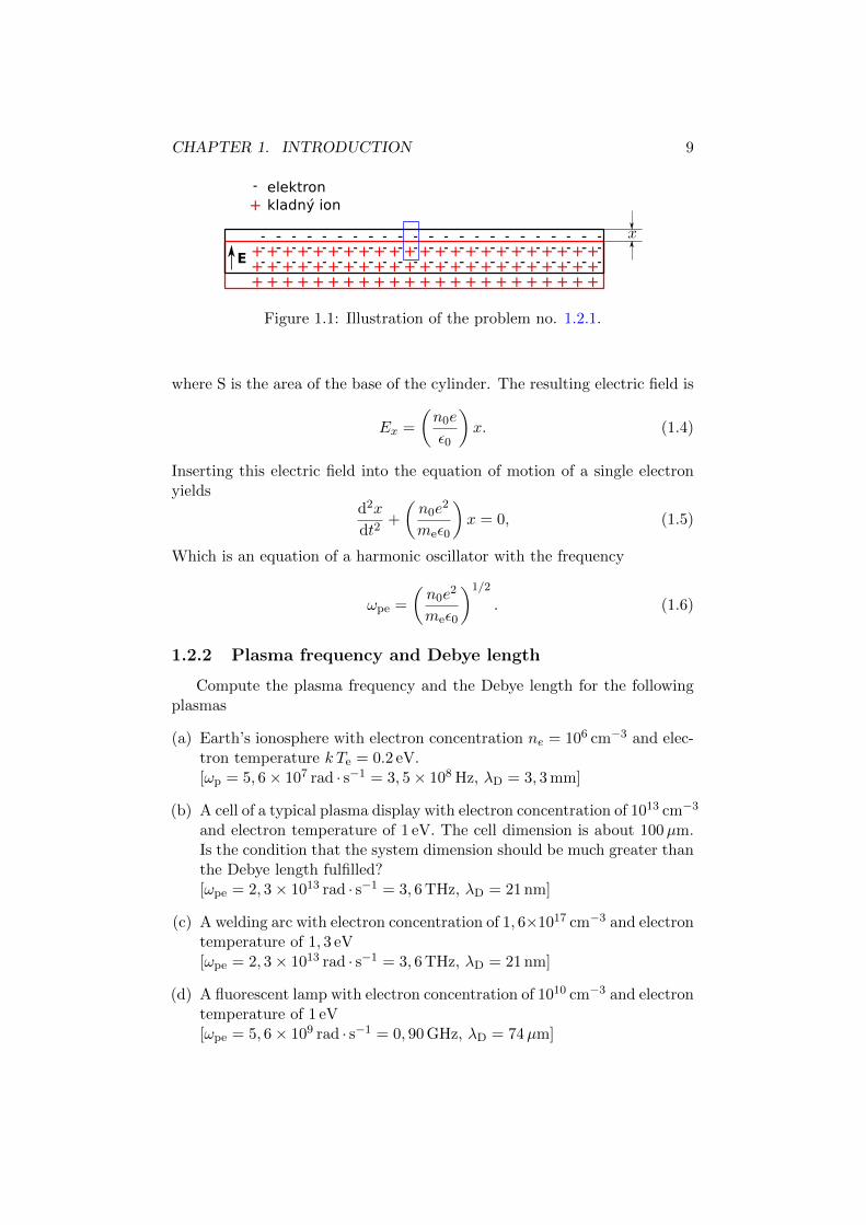
Consider a steady initial state with a uniform number density of electronsand an equal number of ions such that the total electrical charge is neutral.Neglect the thermal motion of the particles and assume that the ions arestationary. Show that a small displacement of a group of electrons leads tooscillations with the plasma frequency according to the equation (1.1).
Solution The situation is sketched in the figure 1.1. Assume that theelectric field in the plane perpendicular to the x-axis is zero (just like inthe case of an infinitely large charged plane or capacitor). Let us apply theGauss’s law to a closed cylindrical surface (only contour of which is sketchedin the figure): ∮
SE · dS =
Q
ε0=
(Snee
ε0
)x, (1.3)
CHAPTER 1. INTRODUCTION 9
Figure 1.1: Illustration of the problem no. 1.2.1.
where S is the area of the base of the cylinder. The resulting electric field is
Ex =
(n0e
ε0
)x. (1.4)
Inserting this electric field into the equation of motion of a single electronyields
d2x
dt2+
(n0e
2
meε0
)x = 0, (1.5)
Which is an equation of a harmonic oscillator with the frequency
ωpe =
(n0e
2
meε0
)1/2
. (1.6)
1.2.2 Plasma frequency and Debye length
Compute the plasma frequency and the Debye length for the followingplasmas
(a) Earth’s ionosphere with electron concentration ne = 106 cm−3 and elec-tron temperature k Te = 0.2 eV.[ωp = 5, 6× 10⁷ rad · s−1 = 3, 5× 10⁸ Hz, λD = 3, 3 mm]
(b) A cell of a typical plasma display with electron concentration of 1013 cm−3
and electron temperature of 1 eV. The cell dimension is about 100µm.Is the condition that the system dimension should be much greater thanthe Debye length fulfilled?[ωpe = 2, 3× 10¹³ rad · s−1 = 3, 6 THz, λD = 21 nm]
(c) A welding arc with electron concentration of 1, 6×1017 cm−3 and electrontemperature of 1, 3 eV[ωpe = 2, 3× 10¹³ rad · s−1 = 3, 6 THz, λD = 21 nm]
(d) A fluorescent lamp with electron concentration of 1010 cm−3 and electrontemperature of 1 eV[ωpe = 5, 6× 10⁹ rad · s−1 = 0, 90 GHz, λD = 74µm]
CHAPTER 1. INTRODUCTION 10
1.2.3 Debye-Huckel potential
Show that Debye–Huckel potential
ϕ(r) =e
4π ε0
exp(− rλD
)r
(1.7)
is solution of equation
∇2ϕ(r) =ϕ(r)
r2D
=ne e
2
ε0kTeϕ(r) (1.8)
where rD is Debye–Huckel radius.Remark: Debye–Huckel potential which is called after Pieter Debye
(1884-1966) and Erich Huckel (1896-1980) who studied polarisation effectsin electrolytes [9].
Solution Put simply the Debye-Huckel potential into the equation (1.8)and calculate Laplace operator in spherical coordinates
∆f =1
r2
∂
∂r
(r2∂f
∂r
)+
1
r2 sin θ
∂
∂θ
(sin θ
∂f
∂θ
)+
1
r2 sin2 θ
∂2f
∂ϕ2(1.9)

Chapter 2
Motion of particles inelectromagnetic fields
2.1 Theory
The Lorentz force is the combination of electric and magnetic force ona point charge due to electromagnetic fields. If a particle of charge q moveswith velocity v in the presence of an electric field E and a magnetic field B,then it will experience the Lorentz force
F = q (E + v ×B) . (2.1)
The gyroradius (also known as Larmor radius or cyclotron radius) isthe radius of the circular motion of a charged particle in the presence of auniform magnetic field:
rg =mv⊥|q|B
, (2.2)
where rg is the gyroradius, m is the mass of the charged particle, v⊥ is thevelocity component perpendicular to the direction of the magnetic field, qis the charge of the particle, and B is magnitude of the constant magneticfield.
Similarly, the frequency of this circular motion is known as the gyrofre-quency or cyclotron frequency, and is given by:
ωg =|q|Bm
. (2.3)
Note: A cyclotron is a type of particle accelerator in which charged particlesaccelerate due to high-frequency electric field. The cyclotron was inventedand patented by Ernest Lawrence of the University of California, Berkeley,where it was first operated in 1932.
11
CHAPTER 2. MOTIONOF PARTICLES IN ELECTROMAGNETIC FIELDS12
2.2 Problems
2.2.1 Magnetic mirror
Magnetic mirrors are used to confine charged particles in a limited vol-ume. The gradient of magnetic field induction can result in reversing thedirection of drift of a charged particle.
Suppose we have an electron located at z = 0 with initial velocity v0 andan initial pitch angle ϑ. The magnetic field induction is given by
B(z) = B0
(1 + (γ z)2
). (2.4)
Calculate the turning point zt [13].
Solution We start with the conservation of kinetic energy and the mag-netic moment. The kinetic energy conservation condition yields
v20 = v2
t . (2.5)
The z-component of the velocity at the turning point must be zero, which weimmediately use in the equation describing the conservation of the magneticmoment
me v20 sin2 ϑ
2B0=
me v2t
2B0 (1 + (γ zt)2)
v20 sin2 ϑ
(1 + (γ zt)
2))
= v2t
(= v2
0
)γ2 z2
t =1− sin2 ϑ
sin2 ϑ
zt =1
γ tanϑ. (2.6)
We see that the position of the point of reflection depends only on thegradient of the magnetic field and on the initial pitch angle.
2.2.2 Magnetic mirror of a different construction
Calculate the turning point for a charged particle in a magnetic mirrorwith induction given by
B(z) = B0
(1 + (γ z)4
). (2.7)
The initial pitch angle is ϑ.[zt =
(1
γ tanϑ
)1/2]
CHAPTER 2. MOTIONOF PARTICLES IN ELECTROMAGNETIC FIELDS13
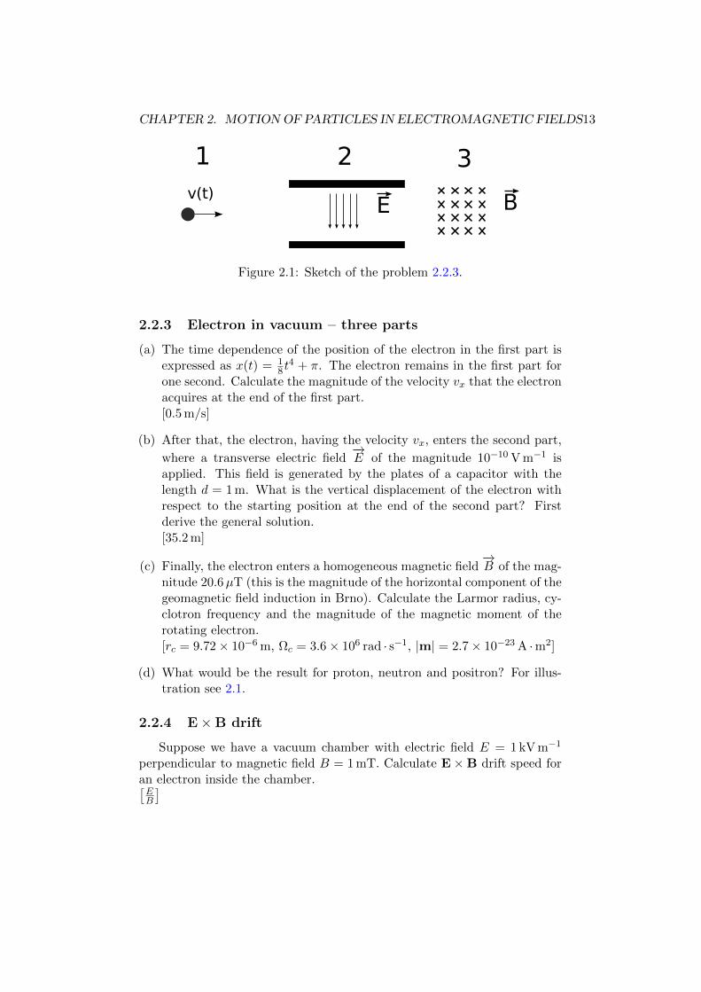
Figure 2.1: Sketch of the problem 2.2.3.
2.2.3 Electron in vacuum – three parts
(a) The time dependence of the position of the electron in the first part isexpressed as x(t) = 1
8 t4 + π. The electron remains in the first part for
one second. Calculate the magnitude of the velocity vx that the electronacquires at the end of the first part.[0.5 m/s]
(b) After that, the electron, having the velocity vx, enters the second part,
where a transverse electric field−→E of the magnitude 10−10 V m−1 is
applied. This field is generated by the plates of a capacitor with thelength d = 1 m. What is the vertical displacement of the electron withrespect to the starting position at the end of the second part? Firstderive the general solution.[35.2 m]
(c) Finally, the electron enters a homogeneous magnetic field−→B of the mag-
nitude 20.6µT (this is the magnitude of the horizontal component of thegeomagnetic field induction in Brno). Calculate the Larmor radius, cy-clotron frequency and the magnitude of the magnetic moment of therotating electron.[rc = 9.72× 10⁻⁶ m, Ωc = 3.6× 10⁶ rad · s−1, |m| = 2.7× 10⁻²³ A ·m2]
(d) What would be the result for proton, neutron and positron? For illus-tration see 2.1.
2.2.4 E×B drift
Suppose we have a vacuum chamber with electric field E = 1 kV m−1
perpendicular to magnetic field B = 1 mT. Calculate E×B drift speed foran electron inside the chamber.[EB
]
CHAPTER 2. MOTIONOF PARTICLES IN ELECTROMAGNETIC FIELDS14
2.2.5 Relativistic cyclotron frequency
What is the relativistic cyclotron frequency of an electron with velocity 0.8 c(c denotes speed of light)?[ω = 6
10 eB/m]
2.2.6 Relativistic particle in an uniform magnetic field
Derive the gyroradius, angular gyrofrequency Ωrelc , and energy of rela-
tivistic particle with speed v and charge q in an uniform magnetic field withmagnitude of magnetic induction B.
Solution Gyroradius:
r =γβm0c
qB(2.8)
Angular gyrofrequency:
Ωrelc =
|q|Bγm0
=Ωc
γ= Ωc
√1− β2 = Ωc
√1−
(vc
)2(2.9)
Energy:
Ek = mγc2 −mc2 =mc2√
1− v2/c2−mc2 (2.10)
2.2.7 Law of conservation of electric charge
Derive continuity equation from Maxwell’s Equations.[∂ρ∂t +∇ · J = 0
]2.2.8 Magnetostatic field
Proof, that in presence of magnetostatic field total kinetic energy ofcharged particle Wk remains constant.
2.2.9 Cyclotron frequency of electron
What is a cyclotron frequency (in Hz) of electron in homogenous magneto-static field:a) | ~B| = 0.01 Tb) | ~B| = 0.1 Tc) | ~B| = 1 Td) | ~B| = 5 T[a) 0.28 GHz ; b) 2.8 GHz; c) 28 GHz d) 140 GHz]
CHAPTER 2. MOTIONOF PARTICLES IN ELECTROMAGNETIC FIELDS15
2.2.10 Cyclotron frequency of ionized hydrogen atom
What is a cyclotron frequency (in Hz) of ionized hydrogen atom in homoge-nous magnetostatic field:a) | ~B| = 0.01 Tb) | ~B| = 0.1 Tc) | ~B| = 1 Td) | ~B| = 5 T[a) 0.15 MHz ; b) 1.5 MHz; c) 15 MHz d) 76 MHz]
2.2.11 Magnetic moment
Suppose a planar closed circular current loop has area |S| = 10−3 m2 andcarries an electric current:a) I = 1 Ab) I = 2 Ac) I = 8 ACalculate the magnitude of its magnetic moment |m|.[a) |m| = 10−3 A m2; b) |m| = 2× 10⁻³ A m2; c)|m| = 8× 10⁻³ A m2 ]
2.2.12 Magnetic moment 2
How can be written the magnitude of the magnetic moment |~m|, which isassociated with the circulating current of charged particle (charge q, angularfrequency ~Ωc, mass m) in uniform magnetostatic field ~B?
[|~m| = |q| | ~Ωc|2π π r2
c ; | ~Ωc| = |q| | ~B|m ]
2.2.13 Lorentz force
Suppose a magnetostatic field ~B = (1, 2, 0) T. The velocity of an electron is~v = (0, 2, 1) m s−1. Calculate Lorentz force.[~F = −e · (−2, 1,−2) N]

Chapter 3
Elements of plasma kinetictheory
3.1 Theory
• Phase space is defined by six coordinations (x, y, z, vx, vy, vz).
• The dynamical state of each particle is appropriately represented by asingle point in this phase space.
• The distribution function in phase space, fα(~r,~v, t), is defined as thedensity of representative points of the particles α in phase space:
fα(~r,~v, t) = N6α(~r,~v, t)/(d3r d3v). (3.1)
• The number density, nα(~r, t), can be obtained by integrating fα(~r,~v, t)over all of velocity space:
nα(~r, t) =
∫~vfα(~r,~v, t)d3v (3.2)
• The differential kinetic equation that is satisfied by the distributionfunction, is generally known as the Boltzmann kinetic equation:
∂fα(~r,~v, t)
∂t+ ~v · ∇~r fα(~r,~v, t) +~a · ∇~v fα(~r,~v, t) =
∂fα(~r,~v, t)
∂t
∣∣∣collision
(3.3)
16

CHAPTER 3. ELEMENTS OF PLASMA KINETIC THEORY 17
3.2 Problems
3.2.1 Uniform distribution function
Suppose we have system of particles uniformly distributed in space with con-stant particle number density n, which is characterised by one dimensionaldistribution function of speeds F (v):
F (v) = C for v ≤ v0
F (v) = 0 otherwise,
where C is positive non-zero constant. Express C using n and v0.
[Solution: By integration n = Cv0∫0
dv we will get the solution C = nv0
.]
3.2.2 Linear distribution function
What is the normalizing constant C of the following distribution functionof speeds?F (v) = C v for v ∈ 〈0, 1〉 and F (v) = 0 otherwise.[C = 2n (n denotes the particle density)]
3.2.3 Quadratic distribution function
What is normalizing constant C of following distribution function of speeds?F (v) = C v2 for v ∈ 〈0, 3〉 and F (v) = 0 otherwise.[C = n/9 (n denotes the particle density)]
3.2.4 Sinusoidal distribution function
What is the normalizing constant C of the following distribution functionof speeds?F (v) = C sin(v) for v ∈ 〈0, π〉 and F (v) = 0 otherwise.[C = n/2 (n denotes the particle density)]
3.2.5 Boltzmann kinetic equation
Consider the motion of charged particles, in one dimension only, in thepresence of an electric potential ϕ(x). Show, by direct substitution, that afunction of the form
f = f
(1
2mv2 + q ϕ(x)
)is a solution of the Boltzmann equation under steady state conditions.

Chapter 4
Average values andmacroscopic variables
4.1 Theory
• The macroscopic variables, such as number density, flow velocity, ki-netic pressure or thermal energy flux can be considered as averagevalues of physical quantities, involving the collective behaviour of alarge number of particles. These macroscopic variables are related tothe various moments of the distribution function.
• With each particle in the plasma, we can associate some molecularproperty χα(~r,~v, t). This property may be, for example, the mass, thevelocity, the momentum, or the energy of the particle.
• The average value of the property χα(~r,~v, t) for the particles of typeα is defined by
〈χα(~r,~v, t)〉 =1
nα(~r, t)
∫~vχα(~r,~v, t)fα(~r,~v, t) d3v. (4.1)
• For example, the average velocity (or flow velocity) ~uα(~r, t) for theparticles of type α is defined by
~uα(~r, t) = 〈vα(~r, t)〉 =1
nα(~r, t)
∫~v~v fα(~r,~v, t) d3v. (4.2)
18

CHAPTER 4. AVERAGE VALUES ANDMACROSCOPIC VARIABLES19
4.2 Problems
4.2.1 RMS speed
What is the rms speed of the following three electrons (|v1| = 1, |v2| = 2and |v3| = 5)?[√
10]
4.2.2 Mean speed of sinusoidal distribution
What is the mean speed of the following distribution function of speeds?f(v) = n
2 sin(v) for v ∈ 〈0, π〉 and f(v) = 0 otherwise. n denotes the particledensity.[1]
4.2.3 Mean speed of quadratic distribution
What is the mean speed of the following distribution function of speeds?f(v) = 3n v2 for v ∈ 〈0, 1〉 and f(v) = 0 otherwise n denotes the particledensity.[3/4]
4.2.4 The equilibrium temperature
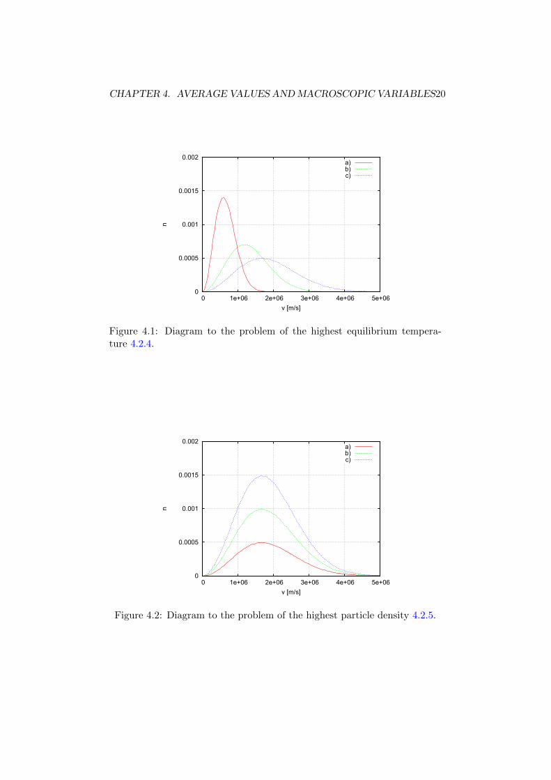
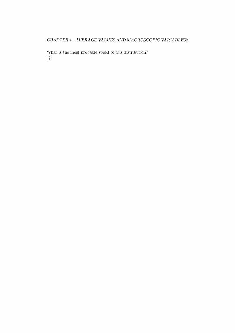
Consider Maxwell-Boltzmann distributions in Fig. 4.1. Which one has thehighest equilibrium temperature?[c)]
4.2.5 Particle density
Consider Maxwell-Boltzmann distributions in Fig. 4.2. Which one has thehighest particle density?[c)]
4.2.6 Most probable speed of linear distribution
Consider the following distribution function of speeds f(v) = n v for v ∈〈0, 1〉 and f(v) = 0 otherwise.What is the most probable speed of this distribution?[1]
4.2.7 Most probable speed of sinusoidal distribution
Consider the following distribution function of speeds f(v) = 12 sin(v) for
v ∈ 〈0, π〉 and f(v) = 0 otherwise.
CHAPTER 4. AVERAGE VALUES ANDMACROSCOPIC VARIABLES20
0
0.0005
0.001
0.0015
0.002
0 1e+06 2e+06 3e+06 4e+06 5e+06
n
v [m/s]
a)b)c)
Figure 4.1: Diagram to the problem of the highest equilibrium tempera-ture 4.2.4.
0
0.0005
0.001
0.0015
0.002
0 1e+06 2e+06 3e+06 4e+06 5e+06
n
v [m/s]
a)b)c)
Figure 4.2: Diagram to the problem of the highest particle density 4.2.5.
CHAPTER 4. AVERAGE VALUES ANDMACROSCOPIC VARIABLES21
What is the most probable speed of this distribution?[π2 ]

Chapter 5
The equilibrium state
5.1 Theory
• The equilibrium distribution function fEqα (~r,~v, t) is the time-independentsolution of the Boltzmann equation in the absence of external forces.
• In the equilibrium state the particle interactions do not cause anychanges in fEqα (~r,~v, t) with time and there are no spatial gradients inthe particle number density.
• fEqα (~r,~v, t) is known as the Maxwell–Boltzmann distribution or Maxwelldistribution (see problems 5.2.2–5.2.4).
Math useful for calculationsThe ”Gaussian integral” is the integral of the Gaussian function e−x
2over
the entire real line. It is named after the German mathematician and physi-cist Carl Friedrich Gauss. The integral is (a, b denotes a constant):∫ +∞
−∞e−x
2dx =
√π;
∫ ∞−∞
e−a(x+b)2 dx =
√π
a. (5.1)
The gamma function Γ(n) is an extension of the factorial function, with itsargument shifted down by 1, to real and complex numbers. That is, if n isa positive integer:
Γ(n) = (n− 1)! (5.2)
Other important formulas:∫ ∞0
xne−a x2dx =
Γ( (n+1)2 )
2 a(n+1)
2
; Γ
(1
2
)=√π. (5.3)
22

CHAPTER 5. THE EQUILIBRIUM STATE 23
5.2 Problems
5.2.1 Gamma function
Starting from the definition of a Gamma function show that, if n is a positiveinteger, then
Γ(n+ 1) = n!
Recipe: First, using integration by parts of Γ(n+1) =∫∞
0 xne−x dx demon-strate that
Γ(a+ 1) = aΓ(a).
Next, it remains to show, that Γ(1) = 1.
5.2.2 1D Maxwell-Boltzmann distribution function
Gas composing of particles of one kind moving in only one dimension xis characterised by the following homogeneous isotropic one-dimensionalMaxwell-Boltzmann distribution function:
f(vx) = C · exp
[−mv2
x
2kT
]. (5.4)
(a) Calculate the constant C.
(b) Derive the 1D Maxwell-Boltzmann distribution function of speeds.
(c) Calculate the most probable speed.
(d) Calculate the mean speed.
(e) Derive the relation for the number of particles passing through a unitof length in a unit of time from one side (the flux of particles from oneside).
Solution
(a) Integrate the distribution function over the whole velocity space. Thecondition that the integral equals the concentration of particles n yields
n = C
∞∫−∞
exp
[−mv2
x
2kT
]dvx = C
√2kTπ
m. (5.5)
C = n
√m
2kTπ(5.6)

CHAPTER 5. THE EQUILIBRIUM STATE 24
(b) Distribution of particle speeds F (v) from the summation over the bothpossible directions is
F (v) = 2n
√m
2kTπexp
[−mv2
2kT
](5.7)
(c) From the condition that the derivation of the distribution F (v) mustequal zero
0 = v exp
[−mv2
2kT
](5.8)
we will get that the most probable speed is zero.
(d)
〈v〉 =
∞∫0
v F (v) dv =
√2kT
πm(5.9)
(e)
Γ =
∞∫0
vx f(vx)dvx = n
√kT
2πm(5.10)
5.2.3 Two-dimensional Maxwell-Boltzmann distribution func-tion
Solve the tasks of the preceding problem with two-dimensional Maxwell-Boltzmann distribution function
f(vx, vy) = C · exp
[−m (v2
x + v2y)
2kT
]. (5.11)
Results:
(a) C = mn2π k T
(b) F (v) = 2π v f(v) = nmk T v exp
[−mv2
2kT
](c) Most probable speed v =
√k Tm .
(d) Mean speed 〈v〉 =√
k T π2m .
(e) Γ = n√
k T2mπ

CHAPTER 5. THE EQUILIBRIUM STATE 25
5.2.4 Three-dimensional Maxwell-Boltzmann distribution func-tion
Solve the tasks of the preceding problem with three-dimensional Maxwell-Boltzmann distribution function
f(vx, vy, vz) = C · exp
[−m (v2
x + v2y + v2
z)
2kT
]. (5.12)
Results:
(a) C = n(
m2π k T
)3/2(b) F (v) = 4π n
(m
2πkT
)3/2v2 exp
[−mv2
2kT
](c) Most probable speed v =
√2 k Tm .
(d) Mean speed 〈v〉 =√
8 k Tπm .
(e) Γ = n√
k T2mπ
5.2.5 Exotic one-dimensional distribution function
Solve the tasks of the preceding problem with the following function (Cauchy/Lorentzdistribution):
f(v) =C
v2 + kTm
. (5.13)
Results:
(a) C = n√
kTmπ2
(b) F (v) = 2n√
kTmπ2
1v2+ kT
m
(c) Most probable v = 0 speed.
(d) Mean speed v is not defined, [1] see Cauchy distribution.
(e) Not defined.

Chapter 6
Particle interactions inplasmas
6.1 Theory
Collisional phenomena can be divided into two categories:
• elastic - conservation of mass, momentum and energy is valid in sucha way that there are no changes in the internal states of the particlesinvolved and there is neither creation nor annihilation of particles.
• inelastic - the internal states of some or all of the particles involved arechanged and particles may be created as well as destroyed. A chargedparticle may recombine with another to form a neutral particle or itcan attach itself to a neutral particle to form a heavier charged particle.The energy state of an electron in an atom may be raised and electronscan be removed from their atoms resulting in ionization.
The total scattering cross section can be obtained by integrating σ(χ, ε)dΩover the entire solid angle:
σt =
∫Ω
σ(χ, ε)dΩ. (6.1)
In the special case, when the interaction potential is isotropic (e.g. Coulombpotential), we can get the total scattering cross section using the formula
σt = 2π
π∫0
σ(χ) sinχdχ. (6.2)
For the same case, when the interaction potential is isotropic, we can getthe momentum transfer cross section using the formula:
26

CHAPTER 6. PARTICLE INTERACTIONS IN PLASMAS 27
σm = 2π
π∫0
(1− cosχ)σ(χ) sinχdχ. (6.3)
6.2 Problems
6.2.1 Mean free path of Xe ions
Scattering cross section σ for elastic collisions of Xe+ ions with Xe atomsis approximately independent on their energy with cross section value ofσ = 10−14 cm2.
A) Calculate mean free path l of Xe+ ions for elastic collisions in a weaklyionized plasma in xenon atmosphere at room temperature (20 C) at thepressure:a) 1000 Pab) 10 Pac) 0.1 Pa
B) How long is the time period between two subsequent collisions, if themean temperature of Xe ions is T = 1000 K?
Solution:
A) The mean free path is defined as
λ =1
nσ.
Density of particles can be calculated from the equation of state p = nk T ,so
λ =k T
p σ.
So the final results for given pressures are:
a) 4 · 10−6 m b) 4 · 10−4 m c) 4 · 10−2 m.
B) The thermal velocity of ions is v =√
3 k TM . Mass of Xe ion is approx-
imately 131 amu (1 amu = 1.66 · 10−27 kg). The time period between twosubsequent collisions equals to the fraction of mean free path and thermal

CHAPTER 6. PARTICLE INTERACTIONS IN PLASMAS 28
velocity:
τ = λ
√m
3 k T.
So the results are: a) 17 · 10−9 s b) 17 · 10−7 s c) 17 ·10−5 s.
6.2.2 Hard sphere model
What is the total scattering cross section for the hard sphere model (twoelastic spheres, radius R1 and R2)?[π (R1 +R2)2]
6.2.3 Total scattering cross section
Differential cross section is given by
σ(χ) =1
2σ0(3 cos2 χ+ 1) (6.4)
Calculate the total cross section and the momentum transfer cross section.[4π σ0, 4π σ0]

Chapter 7
Macroscopic transportequations
7.1 Theory
From different moments of Boltzmann equation, the following macro-scopic transport equations can be derived:
• From the condition of conservation of mass the continuity equation
∂ρmα∂t
+∇ · (ρmαuα) = Sα, (7.1)
where ρmα is the mass density of type-α particles and Sα describesthe creation or destruction of particles due to collisions (ionization,recombination, etc.).
• From conservation of momentum the momentum transfer equation
ρmαDuαDt
= nαqα (E + uα ×B) + ρmαg−∇ · Pα + Aα − uα Sα (7.2)
uα is the mean velocity, DDt = ∂
∂t + uα · ∇ is the total time derivativeoperator, nα is the particle density, qα is the charge of a single particle,E and B are the electric and magnetic fields, g is the gravitationalacceleration, Pα is the kinetic pressure dyad,
Aα = −ρmα∑β
ναβ(uα − uβ) (7.3)
is the collision term with ναβ being the collision frequency for themomentum transfer between the particles of type α and particles oftype β. From conservation of momentum during a collision follows
ρmα ναβ = ρmβ νβα. (7.4)
29
CHAPTER 7. MACROSCOPIC TRANSPORT EQUATIONS 30
• From the energy conservation the energy transport equation
D
Dt
(3 pα
2
)+
3 pα2∇ · uα + (P · ∇) · uα +∇ · qα =
= Mα − uα ·Aα +1
2u2α Sα, (7.5)
where pα is the scalar pressure, qα is the heat flux vector and Mα
represents the rate of energy density change due to collisions.
7.2 Problems
7.2.1 Afterglow
Consider a homogeneous plasma afterglow consisting of electrons and onetype of singly charged positive ions. In this case, the continuity equation is
∂ne∂t
= −kr ne ni, (7.6)
where kr is the rate coefficient for recombination. The spatial derivativesvanish because of the spatial uniformity. The concentration of electrons att = 0 is n0. Calculate ne(t > 0). Remember the quasineutrality condition.[ne(t) = n0
n0 kr t+1
]7.2.2 Macroscopic collision term – momentum equation
Consider a uniform mixture of different fluids (all spatial derivativesvanish), with no external forces, so that the equation of motion for the αspecies reduces to
duαdt
= −ναβ (uα − uβ). (7.7)
Assume that the mass density of β species is much greater and thus neglectthe temporal change of uβ. Notice that at equilibrium (duα/dt = 0) thevelocities of all species must be the same.
solution The situation is identical in all spatial coordinates, thus, onlythe solution in the x direction will be presented.
duαx(t)
dt+ ναβuαx(t) = ναβ uβx (7.8)
This simple differential equation can be solved by the method of variationof parameter. First, look for the particular solution of the homogeneousequation
duαx,p(t)
dt+ ναβuαx,p(t) = 0 (7.9)
CHAPTER 7. MACROSCOPIC TRANSPORT EQUATIONS 31
This is obviouslyuαx,p(t) = C e−ναβt (7.10)
We now take the parameter C to be time-dependent C = C(t) and calculatethe deriative
duαx(t)
dt=
dC(t)
dte−ναβt − C(t) ναβe−ναβt (7.11)
inserting this into the original equation (7.8) yields
dC(t)
dte−ναβt = ναβ uβx
from which we obtain by integrating
C(t) = uβx eναβ t +K
where K is an arbitrary integration constant. The solution is then
uαx(t) = uβx +K e−ναβ t (7.12)
And similarly for all three spatial components. The velocity uα will expo-nentially approach to the velocity uβ with the rate given by the collisionfrequency for momentum transfer ναβ.
7.2.3 Macroscopic collision – momentum equation II
Recalculate the task of the previous problem without the assumptionuβ = const. In this case, the velocities uα, uβ are described by a pair ofcoupled differential equations
duα(t)
dt= −ναβ (uα(t)− uβ(t)). (7.13)
duβ(t)
dt= −ρmα
ρmβναβ (uβ(t)− uα(t)), (7.14)
where ρmα, ρmβ are the mass densities of particles α, β. Suppose that uαand uβ are parallel and uα(t = 0) = 2uβ(t = 0).
(a) Calculate the time dependence of the difference u = uα − uβ.
(b) Calculate uα(t) and uβ(t).
Results:
(a) u(t) = uα(0) · exp[(
1 + ρmαρmβ
)t]
(b) uα(t) = uα(0)ρmα+ρmβ
(ρmβ · exp
[−ναβ
(1 + ρmα
ρmβ
)t]
+ ρmα
)uβ(t) = u(t) + uα(t)

CHAPTER 7. MACROSCOPIC TRANSPORT EQUATIONS 32
7.2.4 Simplified heat flow equation
Suppose the simplified equation for heat flow in a stationary electron gas
5 pe2∇(peρme
)+ Ωce (qe ×B) =
(δqe
δt
)coll
. (7.15)
Assume the collision term given by the relaxation model(δqe
δt
)coll
= −ν (fe − fe0) (7.16)
and the ideal gas law pe = ne k Te. Show that the heat flow equation can bewritten as
Ωce
ν(qe ×B) = −K0∇Te + (fe − fe0), (7.17)
where
K0 =5 k pe2me ν
(7.18)
is the thermal conductivity.

Chapter 8
Macroscopic equations for aconducting fluid
8.1 Theory
The equations governing the important physical properties of the plasmaas a whole can be obtained by summing the terms for the particular species.If also several simplifying assumptions are made, the following set of socalled magnetohydrodynamic equations can be derived:
• The continuity equation
∂ρm∂t
+∇ · (ρmu) = 0 (8.1)
• The momentum equation
ρmDu
Dt= J×B−∇p (8.2)
• Generalised Ohm’s law
J = σ0(E + u×B)− σ0
n eJ×B. (8.3)
The electric and magnetic fields are further bound by the Maxwell equations.In these equations, viscosity and thermal conductivity are neglected.
8.2 Problems
8.2.1 Electric current density
The mean velocity of plasma u is defined as a weighted average of themean velocities of the particular species
u =∑α
ρmαρm
uα (8.4)
33

CHAPTER 8. MACROSCOPIC EQUATIONS FOR A CONDUCTING FLUID34
where ρm is the total mass density of the plasma. Each species has con-centration nα, charge qα and the so called diffusion velocity wα = uα − u.Calculate the total electric current density J in terms of the total electriccharge density ρ and the particular densities, charges and diffusion veloci-ties. Note, that due to the definition of the mean velocity of plasma, theresult is not simply J = ρu.[J = ρu +
∑αnα qαwα
]8.2.2 Fully ionised plasma
From the equation for electric current density in fully ionised plasmacontaining electrons and one type of ions with charge e
J =∑α
nα qα uα = e(ni ui − ne ue) (8.5)
and form the equation for the mean velocity of the plasma as a whole
u =1
ρm(ρme ue + ρmi ui) (8.6)
derive the drift velocities ui and ue.[ui = µ
ρmi
(ρmume
+ Je
), ue = µ
ρme
(ρmumi− J
e
), µ = memi
me+mi
]8.2.3 Diffusion across the magnetic field
From the momentum conservation equation with the magnetohydrody-namic approximation
ρmDu
Dt= J×B−∇p (8.7)
and the generalised Ohm’s law in the simplified form and without consideringthe Hall effect term
J = σ0 (E + u×B) (8.8)
derive the equation for the fluid velocity u.Assume E = 0 and p = const. and calculate the fluid velocity perpen-
dicular to the magnetic field B.
Solution The equation for u is
ρmDu
Dt= σ0 E×B + σ0 (u×B)×B−∇p. (8.9)
Assuming E = 0 and p = const., it reduces to
ρmDu
Dt= σ0 (u×B)×B (8.10)

CHAPTER 8. MACROSCOPIC EQUATIONS FOR A CONDUCTING FLUID35
To calculate the vector (u×B)×B we define the coordinates such thatthe z-axis is parallel with the magnetic field. In these coordinates, the crossproduct is
(u×B)×B = (−uxB2, −uy B2, 0). (8.11)
The equations for x and y component of the velocity are thus of the sameform. Writing only the equation in x
DuxDt
=−σ0B
2
ρmux (8.12)
This has a form of a simple decay problem. The solution is
ux(t) = ux(0) exp
(−σ0B
2
ρmt
). (8.13)
The same holds for uy, so the time dependence of the component of the
velocity perpendicular to the magnetic field u⊥ =√u2x + u2
y is
u⊥(t) = u⊥(0) exp (−t/τ) , (8.14)
whereτ =
ρmσ0B2
(8.15)
is the characteristic time for diffusion across the magnetic field lines.

Chapter 9
Plasma conductivity anddiffusion
9.1 Theory
In weakly ionised cold plasma, the equation of motion for electrons takesthe simple form of the so called Langevin equation
meDueDt
= −e (E + ue ×B)− νcme ue, (9.1)
where νc is the collision frequency for momentum transfer between the elec-trons and the heavy particles.
In the absence of a magnetic field, the current produced by movingelectrons is
J = −e ne ue (9.2)
and the DC conductivity is
σ0 =ne e
2
me νc(9.3)
and the electron mobility
Me = − e
me νc= − σ0
ne e. (9.4)
When an external magnetic field is present, the plasma becomes anisotropic,and the DC conductivity and electron mobility are described by tensors (seeproblem 9.2.2).
In weakly ionised plasma with relatively high density of neutrals, thediffusion equation for charged species α is
∂nα∂t
= D∇2nα. (9.5)
36

CHAPTER 9. PLASMA CONDUCTIVITY AND DIFFUSION 37
The diffusion coefficient De for electrons in an isotropic plasma with nointernal electric fields is
De =k Teme νc
. (9.6)
In the magnetised plasma, the De becomes a tensor similar to the DCconductivity or electron mobility.
In plasma, electrons usually diffuse faster than ions due to their lowermass and thus higher mobility. As a result, internal electric field is produced,slowing down the diffusion of electrons and speeding up the diffusion of ions.This effect is called ambipolar diffusion. If the relation between the ionconcentration ni and ne is
ni = C ne (9.7)
where C is a constant, the ambipolar diffusion coefficient Da is
Da =k (Te + C Ti)
me νce + C mi νci, (9.8)
where νci, νce are the collision frequencies for momentum transfer betweenneutrals and ions or electrons, respectively.
9.2 Problems
9.2.1 DC plasma conductivity
From the Langevin equation for electrons in the absence of magneticfield and in the steady state
− eE−me νc ue = 0 (9.9)
derive the expression for the DC conductivity of the plasma.
Solution The electric current density is defined as
J = −e ne ue (9.10)
Inserting this into the Langevin equation (9.9), we obtain the expression forthe current density J
J =ne e
2
me νcE (9.11)
The Ohm’s law statesJ = σ0 E (9.12)
the DC conductivity is thus
σ0 =ne e
2
me νc. (9.13)
CHAPTER 9. PLASMA CONDUCTIVITY AND DIFFUSION 38
9.2.2 Mobility tensor for magnetised plasma
In magnetised plasma, the Ohm’s law obtains a matrix form
J = S ·E (9.14) JxJyJz
=
σ⊥ −σH 0σH σ⊥ 00 0 σ‖
ExEyEz
,
where the components of the DC conductivity tensor S are
σ⊥ =ν2c
ν2c + Ω2
ce
σ0 (9.15)
σH =νc Ωce
ν2c + Ω2
ce
σ0 (9.16)
σ‖ = σ0 =ne e
2
me νc, (9.17)
where νc is the collision frequency for momentum transfer between electronsand heavy particles and Ωce is the electron cyclotron frequency due to theexternal magnetic field. Find the components of the mobility tensor Me
defined asue =Me ·E. (9.18)
Results:
Me =
M⊥ −MH 0MH M⊥ 0
0 0 M‖
M⊥ = − νc e
me (ν2c + Ω2
ce)(9.19)
MH = − Ωce e
me (ν2c + Ω2
ce)(9.20)
M‖ = − e
me νc(9.21)
9.2.3 Ohm’s law with magnetic field
Consider the equation J = S · E as in the preceding problem. Supposethat E = (E⊥, 0, E‖) and B = (0, 0, B0). Calculate J. Note what directionof the electric current is governed by what component of S.[J = (σ⊥E⊥, σH E⊥, σ‖E‖)
]

CHAPTER 9. PLASMA CONDUCTIVITY AND DIFFUSION 39
9.2.4 Diffusion equation
Solve the diffusion equation for one spatial dimension
∂n(x, t)
∂t= D
∂2n(x, t)
∂x2(9.22)
by separation of variables, assuming
n(x, t) = S(x)T (t). (9.23)
Results:
• Tk(t) = T0 exp(−Dk2 t)
• S(x) = c(k) exp(i k x), k is a separation constant
• n(x, t) =+∞∫−∞
c(k) exp(−i k x−Dk2 t) dk

Chapter 10
Some basic plasmaphenomena
10.1 Theory
In a paper from 1923, an American chemist and physicist wrote, thatelectrons are repelaed from negative electrode, whereas positive ions areattracted towards it. Langmuir concluded, that around every negative elec-trode, a sheath of defined thickness containing only positive ions and neutralatoms exists. Morever, Langmuir observed, that also the glass wall of thedischarge chamber is negatively charged and repels (or reflects) almost allelectrons [16].
The fact, that insulated objects inside plasma are negatively charged(in respect to plasma) to floating potential, is caused by higher mobility ofelectrons than ions. The thermal velocity of electrons (kBTe/me)
1/2 is atleast 100 times higher than the thermal velocity of ions (kBTi/Mi)
1/2 [17].The first reason for different mobility is higher mass of ions. If we consideronly proton (the lightest ion that can appear in a plasma), than the ratiobetween the mass of proton and electron mp/me is 1836. This ratio cor-responds approximately to the ratio of masses of heavy bowling ball (5 kg)and ping pong ball (2,7 g). Another reason for higher thermal velocity ofelectrons in low-temperature plasma is their higher temperature in respectto the ions.
The slowest possible speed of ions at the sheath edge is called the Bohmspeed uB. Ionts are accelerated to this speed in a quasi-neutral pre-sheath,where small electric field exists. The Bohm criterion of plasma sheath isdescribed by following equation
us(0) ≥ uB =
√kB Te
Mi. (10.1)
40

CHAPTER 10. SOME BASIC PLASMA PHENOMENA 41
10.2 Problems
10.2.1 Waves in non-magnetized plasma
Plasma of so called E layer of Earth’s ionosphere has electron density ap-proximately 105 cm−3 and is at altitude of approximatelyo 100 km.a) Which electromagnetic waves can be reflected from this layer?b) Calculate the dielectric constant of plasma for the waves with frequenciesof 100 Mhz and 1000 Hz.b) Calculate the skin depth of the wave with frequency of 1000 Hz.
Solution:
a) All electromagnetic waves with frequency lower than the plasma frequency(2 839 725 Hz) will be reflected.
b) The dielectric constant of plasma is defined as
ε = 1−ω2p
ω2
For 100 MHz ε = 0.9991 (positive value, elmag. waves propagate), for1000 Hz ε = −8064037 (negative value, imaginary refraction index, reflec-tion).
c) Skin depth δ appropriately equals to c/√ω2p − ω2, where c is speed of
light. The skin depth for 1000 Hz is 16.8 m.
10.2.2 Floating potential
Explain why insulated object inserted to plasma will aquire a negative po-tential with respect to the plasma itself.
10.2.3 Bohm velocity
Calculate the Bohm velocity for hydrogen ion in plasma with electron tem-perature of Te = 1 eV.[9 787.2 m/s]
10.2.4 Plasma frequency
When the macroscopic neutrality of plasma is instantaneously perturbed byexternal means, the electrons react in such a way as to give rise to oscillationsat the electron plasma frequency. Consider these oscillations, but includealso the motion of ions. Derive the natural frequency of oscillation of thenet charge density in this case. Use the linearized equations of continuityand of momentum for each species, and Poisson equation, considering only

CHAPTER 10. SOME BASIC PLASMA PHENOMENA 42
the electric force due to the internal charge separation.
[ω = (ω2e + ω2
i )1/2, where ωi =√
ne e2
ε0Mi]
Chapter 11
Boltzmann andFokker-Planck collision terms
11.1 Theory
Under several simplifying assumptions (mainly homogeneous and isotropicdistribution function of electronic velocities, molecular chaos, consideringonly binary collisions and ignoring external forces), so called Boltzmanncollision integral can be derived(
∂f
∂t
)coll
=
∫∫g σ(g,Ω) [fe(v
′) f1(v′1)− fe(v) f1(v1)] dΩ d3v. (11.1)
g = |v − v1| is the relative speed of the electron and its collision partner,σ is the differential cross section for this type of collisions, depending onthe solid angle Ω. Two types of distribution functions are considered here– the electronic distribution function fe(v) and that of the particular kindof collision partners f1(v1). If more kinds of collision partners should beconsidered, the collision term is expressed as a sum of terms similar to eq.(11.1).
The first term expresses the amount of electrons with initial velocity v′
that undergo collisions with the collision partner with velocity v′1. Afterthis collision, the electrons have velocity v and their collision partners havevelocity v1, i.e. they add to the electronic distribution function at thevelocity v. The second term expresses an inverse collision, which leads toloss of particles of the velocity v and is thus negative.
If only collisions leading to small-angle deflections are considered, asexpected for long-range Coulomb interactions, the Fokker-Planck collisionterm can be derived(
δ fαδt
)coll
= −∑i
∂
∂vi(fα〈∆vi〉av)+
1
2
∑ij
∂2
∂vi∂vj(fα〈∆vi∆vj〉av), (11.2)
43

CHAPTER 11. BOLTZMANNAND FOKKER-PLANCK COLLISION TERMS44
where
〈∆vi〉av =
∫Ω
∫v1
∆vi g σ(Ω)dΩfβ1 d3v1 (11.3)
〈∆vi∆vj〉av =
∫Ω
∫v1
∆vi∆vj g σ(Ω)dΩfβ1 d3v1 (11.4)
are the coefficients of dynamical friction and diffusion in velocity space,respectively.
11.2 Problems
11.2.1 Collisions for Maxwell-Boltzmann distribution func-tion
Consider a plasma in which the electrons and the ions are characterised,respectively, by the following distribution functions
fe = n0
(me
2π k Te
)3/2
exp
[−me(v − ue)
2
2 k Te
](11.5)
fi = n0
(mi
2π k Ti
)3/2
exp
[−mi(v − ui)
2
2 k Ti
](11.6)
(a) Calculate the difference (fe(v′) fi(v
′1)− fe(v) fi(v1)).
(b) Show that this plasma of electrons and ions will be in the equilibriumstate, that is, the difference (fe(v
′) fi(v′1) − fe(v) fi(v1)) will vanish if
and only if ue = ui and Te = Ti.
Solution
(a)
(fe(v′) fi(v
′1)− fe(v) fi(v1)) = n2
0
(1
2π k
)3(memi
Te Ti
)3/2
×
×(
exp
[−me (v′ − ue)
2
2 k Te− mi (v′1 − ui)
2
2 k Ti
]−
− exp
[−me (v − ue)
2
2 k Te− mi (v1 − ui)
2
2 k Ti
])(11.7)
(b) For the difference to vanish, the term in the parentheses must equal zero.This will happen if the arguments of the exponentials will be equal. Letus rewrite the arguments, omitting the factor −(2 k)−1:
me
Te(v′2 − 2 v′ · ue + u2
e) +mi
Ti(v′21 − 2 v′1 · ui + u2
i ) (11.8)

CHAPTER 11. BOLTZMANNAND FOKKER-PLANCK COLLISION TERMS45
me
Te(v2 − 2 v · ue + u2
e) +mi
Ti(v2
1 − 2 v1 · ui + u2i ) (11.9)
From the derivation of the Boltzmann collision term follows, that thepairs of velocities v, v1 and v′, v′1 can be considered as pairs of velocitiesbefore and after an elastic two-body collision. Thus, they are bound bythe conservation laws:
me v2 +mi v
21
2=me v
′2 +mi v′21
2(11.10)
me v +mi v1 = me v′ +mi v′1 (11.11)
It is now obvious from the last four equations, that the collision termwill vanish if and only if Te = Ti and ue = ui. In other words, thedistribution function fe will be changed by the collisions only if theplasma is out of equilibrium – the collisions tend to bring the plasma tothe state of equilibrium.
11.2.2 Collisions for different distributions
Recalculate the task (a) of the preceding problem with Druyvesteyn-likedistribution function for electrons and Maxwell-Boltzmann-like distributionfor ions (Ce, ae and Ci are constants)
fe = Ce exp[−aem2e (v − ue)
4] (11.12)
fi = Ci exp
[−mi (v′1 − ui)
2
2 k Ti
](11.13)
Will the difference (fe(v′) fi(v
′1)− fe(v) fi(v1)) be zero for ue = ui?
11.2.3 Collisions for Druyvesteyn distribution
Recalculate task (a) of the first problem for Druyvesteyn-like distributionfor both electron and ion velocities (see eq. (11.12)). Can the collision termbe equal zero for ue = ui? Is it possible to find equilibrium state of plasmadescribed by the Boltzmann kinetic equation with Boltzmann collision termin form of Druyvesteyn-like distribution?

Bibliography
[1] Cauchy distribution. http://en.wikipedia.org/wiki/Cauchy_
distribution. Accessed: 2013-04-10.
[2] Msis-e-90 atmosphere model. http://omniweb.gsfc.nasa.gov/
vitmo/msis_vitmo.html. Accessed: 2013-08-15.
[3] B Bachmann, R Kozakov, G Gott, K Ekkert, J-P Bachmann, J-L Mar-ques, H Schopp, D Uhrlandt, and J Schein. Power dissipation, gastemperatures and electron densities of cold atmospheric pressure he-lium and argon rf plasma jets. Plasma Sources Science and Technology,46(12):125203, 2013.
[4] Jose A Bittencourt. Fundamentals of plasma physics. Springer, 2004.
[5] B Bora, H Bhuyan, M Favre, E Wyndham, and H Chuaqui. Diagnos-tic of capacitively coupled low pressure radio frequency plasma: Anapproach through electrical discharge characteristic.
[6] L Campbell and MJ Brunger. Modelling of plasma processes incometary and planetary atmospheres. Plasma Sources Science andTechnology, 22(1):013002, 2012.
[7] Guangsup Cho and John V Verboncoeur. Plasma wave propagationwith light emission in a long positive column discharge.
[8] Eun Ha Choi, Jeong Chull Ahn, Min Wook Moon, Jin Goo Kim,Myung Chul Choi, Choon Gon Ryu, Sung Hyuk Choi, Tae Seung Cho,Yoon Jung, Guang Sup Cho, et al. Electron temperature and plasmadensity in surface-discharged alternating-current plasma display panels.Plasma Science, IEEE Transactions on, 30(6):2160–2164, 2002.
[9] P Debye and E Huckel. De la theorie des electrolytes. i. abaissement dupoint de congelation et phenomenes associes. Physikalische Zeitschrift,24(9):185–206, 1923.
[10] S Hofmann, AFH van Gessel, T Verreycken, and P Bruggeman. Powerdissipation, gas temperatures and electron densities of cold atmospheric
46
BIBLIOGRAPHY 47
pressure helium and argon rf plasma jets. Plasma Sources Science andTechnology, 20(6):065010, 2011.
[11] J Hubert, M Moisan, and A Ricard. A new microwave plasma at at-mospheric pressure. Spectrochimica Acta Part B: Atomic Spectroscopy,34(1):1–10, 1979.
[12] Zdenek Hubicka. The low temperature plasma jet sputtering systemsapplied for the deposition of thin films. 2012.
[13] Umran S Inan and Marek Go lkowski. Principles of plasma physics forengineers and scientists. Cambridge University Press, 2010.
[14] Jae Duk Kim, Young Ho Na, Young June Hong, Han Sup Uhm,Eun Ha Choi, et al. Microwave plasma jet system development atatmospheric pressure using a 2.45 ghz gan hemt devices. In PlasmaScience (ICOPS), 2011 Abstracts IEEE International Conference on,pages 1–1. IEEE, 2011.
[15] SB Krupanidhi and M Sayer. Position and pressure effects in rf mag-netron reactive sputter deposition of piezoelectric zinc oxide. Journalof applied physics, 56(11):3308–3318, 1984.
[16] I. Langmuir. Positive Ion Currents from the Positive Column of Mer-cury Arcs. Science, 58:290–291, October 1923.
[17] M.A. Lieberman and A.J. Lichtenberg. Principles of plasma dischargesand materials processing. Published by A Wiley-Interscience Publica-tion, page 388, 1994.
[18] Liming Liu, Ruisheng Huang, Gang Song, and Xinfeng Hao. Be-havior and spectrum analysis of welding arc in low-power yag-laser–mag hybrid-welding process. Plasma Science, IEEE Transactions on,36(4):1937–1943, 2008.
[19] Yasuyuki Noguchi, Akira Matsuoka, Kiichiro Uchino, and KatsunoriMuraoka. Direct measurement of electron density and temperaturedistributions in a micro-discharge plasma for a plasma display panel.Journal of applied physics, 91(2):613–616, 2002.
[20] Kunio Okimura, Akira Shibata, Naohiro Maeda, Kunihide Tachibana,Youichiro Noguchi, and Kouzou Tsuchida. Preparation of rutile tio2films by rf magnetron sputtering. JAPANESE JOURNAL OF AP-PLIED PHYSICS PART 1 REGULAR PAPERS SHORT NOTESAND REVIEW PAPERS, 34:4950–4950, 1995.
[21] Cheng-gang PAN, Xue-ming HUA, Wang ZHANG, Fang LI, and XiaoXIAO. Calculating the stark broadening of welding arc spectra byfourier transform method. 32(7), 2012.

BIBLIOGRAPHY 48
[22] Shahid Rauf and Mark J Kushner. Optimization of a plasma displaypanel cell. In APS Annual Gaseous Electronics Meeting Abstracts, vol-ume 1, 1998.
[23] P Sigurjonsson and JT Gudmundsson. Plasma parameters in a planardc magnetron sputtering discharge of argon and krypton. In Journal ofPhysics: Conference Series, volume 100, page 062018. IOP Publishing,2008.
[24] Zemlicka R. In situ studium rustu a leptanı tenkych vrstev vnızkotlakych vysokofrekvencnıch kapacitne vazanych vybojıch. 2012.