Workshop Modelling in Endurance Sports

11.-13. September 2016

University of Konstanz, Germany

PROCEEDINGS

Konstanzer Online-Publikations-System (KOPS) URL: http://nbn-resolving.de/urn:nbn:de:bsz:352-0-371586

ii

Foreword

This book contains the proceedings of the Workshop Modelling in Endurance Sports, which has taken place in Konstanz (Germany) from 11 to 13 September 2016. The workshop was supported by the German Research Foundation (DFG) and the University of Konstanz and co-organized by the University of Konstanz and the German Society of Sport Science (dvs).

In 15 oral presentations, current research topics with focus on modelling in endurance sports like cycling, running and speed skating were discussed. They were organized in four sessions: “Performance Modelling”, “Physiology: VO2, HR, and Lactate”, “Parameter Estimation”, and “Training: Monitoring and Modelling”. Additionally four invited speakers presented their topics of research and in a practical demo session, the workgroup Multimedia Signal Processing of the University of Konstanz presented their Powerbike simulator.

All authors submitted an extended abstract of up to six pages. Each abstract was reviewed by three members of the program committee. The extended abstracts as well as the four short abstracts of the keynote speakers are included in this book. A special issue of the International Journal of Computer Science in Sport (IJCSS) with the topic “Modelling in Endurance Sports” will follow this workshop.

We thank all the participants for making the workshop an inspiring and productive event. Especially, we thank the authors and the invited speakers for their interesting contributions as well as the program committee for helping us with their expertise. Last but not least we also thank our secretaries for their excellent work.

Workshop: https://www.informatik.uni-konstanz.de/saupe/workshop2016/

Sponsors

German Research Foundation

University of Konstanz

iii

Organizers

University of Konstanz

German Society of Sport Science

Local Organizing Committee

Alexander Artiga Gonzalez Ingrid Baiker Raphael Bertschinger Thorsten Dahmen Maciej Gratkowski Dietmar Saupe Claudia Widmann Stefan Wolf

Program Committee

Chris Abbiss (Edith Cowan University, Australia) Arnold Baca (University of Vienna, Austria) Ralph Beneke (Philipps-Universität Marburg, Germany) Thorsten Dahmen (University of Konstanz, Germany) Charles Dauwe (Belgium) Oliver Faude (University of Basel, Switzerland) Andy Froncioni (Alphamantis Technologies, Montreal, Canada) Markus Gruber (University of Konstanz, Germany) Anne Hecksteden (Saarland University, Germany) Andrew Jones (University of Exeter, UK) Grégoire Millet (Université de Lausanne, Switzerland) Jürgen Perl (Mainz, Germany) Kai Röcker (Hochschule Furtwangen, Germany) Dietmar Saupe (University of Konstanz, Germany) Friederike Scharhag-Rosenberger (DHfPG Saarbrücken, Germany) Philip Skiba (Advocate Lutheran General Hospital, Park Ridge, IL, USA) Michael Stöckl (University of Vienna, Austria) David Sundström (Mid Sweden University, Sweden) Guido Vroemen (Sportmedisch Adviescentrum, Netherlands)

iv

Content

Keynote Speakers

Modelling of Fatigue, Function and Performance During Endurance Cycling

Chris Abbiss, Edith Cowan University, Perth, Australia. 1

Modeling Sprint Finishes of Endurance Cycling Competitions Jim Martin, University of Utah, Salt Lake City, USA.

1

Performance Index for Cycling Daniel Green, Trek-Segafredo Cycling Team.

2

Practical Applications of Simulation & Optimisation in Road Cycling Rob Kitching, www.cyclingpowerlab.com, London, UK.

2

Performance Modelling

Predicting performance from outdoor cycling training with the fitness-fatigue model

Melanie Ludwig, Bonn-Rhein-Sieg University of Applied Sciences, Germany Alexander Asteroth, Bonn-Rhein-Sieg University of Applied Sciences, Germany

3

4-parameter critical power model for optimal pacing strategies in road cycling Thorsten Dahmen, University of Konstanz, Germany

7

A practical investigation of optimal strategies on the Fluela pass Stefan Wolf, University of Konstanz, Germany Raphael Bertschinger, University of Konstanz, Germany

11

Two body dynamic model for speed skating driven by the skaters leg extension Eline van der Kruk, Delft University of Technology, The Netherlands Dirkjan H.E.J. Veeger, Delft University of Technology, The Netherlands Frans C.T. van der Helm, Delft University of Technology, The Netherlands Arend L. Schwab, Delft University of Technology, The Netherlands

14

Predicting maximum speed in a 4x1000 m field test based on estimated VO2max values from Shuttle-Run-Test and Queens-College-Step-Test

Jörg M. Jäger, Justus-Liebig-University Gießen, Germany Johannes Kurz, Justus-Liebig-University Gießen, Germany Hermann Müller, Justus-Liebig-University Gießen, Germany

20

Determination of critical speed and the running distance above critical speed under laboratory and field conditions using equal exhaustive durations

Christoph Triska, University of Vienna, Austria Bettina Karsten, University of Greenwich, UK Harald Tschan, University of Vienna, Austria Alfred Nimmerichter, University of Applied Sciences Wr. Neustadt, Austria

25

Ball (not) in play: the distortive effect of net playing time on the decline of match running performance in professional football

Daniel Linke, Technical University Munich, Germany Martin Lames, Technical University Munich, Germany

29

v

Physiology: VO2, HR, and Lactate

Prediction of individual short term heart rate responses

Katrin Hoffmann, Technische Universität Darmstadt, Germany 31

A comparison of models for oxygen consumption Alexander Artiga Gonzalez, University of Konstanz, Germany

34

Modelling the acute physiological response to cycling exercise: the blood lactate concentration challenge

Andrea Zignoli, University of Verona, Italy Alessandro Fornasiero, University of Verona, Italy Matteo Morelli, University of Trento, Italy Francesco Biral, University of Trento, Italy Enrico Bertolazzi, University of Trento, Italy Barbara Pellegrini, University of Verona, Italy Federico Schena, University of Verona, Italy

40

Parameter Estimation

The evolution over 4 years of a female cycling champion is revealed by the Athlete Performance Passport

Charles Dauwe, Gent University, Belgium Johan Strobbe, www.iQO2.com

44

Comparing Opposing Force Power Meters with SRM Raman Garimella, University of Konstanz, Germany

47

Training: Monitoring and Modelling

Modeling altitude training benefits with the record power profile in professional cyclists

Samuel Bellenoue, University of Lausanne, Switzerland Jean-Baptiste Quiclet, 2AG2R-La Mondiale Pro Cycling Team, France Grégoire Millet, University of Lausanne, Switzerland

50

Comparison between maximal lactate steady-state, critical power and the second ventilatory threshold detected by a computer algorithm

Raphael Bertschinger, University of Konstanz, Germany Patrick Thumm, University of Konstanz, Germany Maciej Gratkowski, University of Konstanz, Germany Alexander Artiga Gonzalez, University of Konstanz, Germany Dietmar Saupe, University of Konstanz, Germany.

54

High cycling cadences allow for an increase in training volume monitored via blood lactate concentration

Ralph Beneke, Philipps University Marburg, Germany Renate M. Leithäuser, Philipps University Marburg, Germany

57

Modelling of Fatigue, Function and Performance During Endurance Cycling

Chris Abbiss, Edith Cowan University, Australia.

Many methods and techniques have been developed in order to model endurance performance. Such modelling provides valuable information regarding the quantification of load during both training and competition. This quantification is of importance to understanding fitness and fatigue and thus hopefully assist in the prediction of both optimal (i.e. competition) and suboptimal (i.e. overreaching) performances. However, the modelling of performance in endurance sports is often complicated by difficulties in the quantification of input and output variables to these models. This presentation will discuss some of these issues in the quantification of load during prolonged exercise.

Modeling Sprint Finishes of Endurance Cycling Competitions

Jim Martin, Associate Professor, University of Utah, USA.

Endurance cycling events are often won or lost in a maximal finishing sprint. Supply and demand modeling may provide useful insight regarding optimal sprinting strategies. However, modeling energy supply during such a sprint is complicated by the initial conditions for that sprint, including fatigue and pedaling rate, and by the progression of fatigue during the sprint itself. Energy demand is highly dependent on aerodynamic drag which, in turn, depends on velocity and proximity to other riders. In this presentation, validation of a recently-developed model for supply power during maximal cycling will be presented. An established demand model will be modified to include recently published data on rider-rider aerodynamic interactions. These supply and demand models will be coupled to predict performance using forward integration and to explore a variety of sprint finish strategies including starting point, gear selection, following distance, and lateral clearance during passing.

1

Performance Index for Cycling

Daniel Green, Trek-Segafredo Cycling Team.

In order to evaluate if an athlete is adapting and improving to a training stimulus it is essential to have a method to assess performance. Due to the highly stochastic nature of road cycling, the attributes essential to achieving results requires athletes to produce high power outputs for durations as short as 3 seconds, or for more than 40 minutes. Therefore a new methodology has been devised which calculates a Performance Index for Cycling (PIC). The PIC is single metric which is representative of the performance capabilities of a cyclist across a range of time durations and racing circumstances. The PIC can then be used to monitor changes within a single cyclists or to compare cyclists with different attributes in order to assess their potential for success in road cycling.

Practical Applications of Simulation & Optimisation in Road Cycling

Rob Kitching, www.cyclingpowerlab.com, London, UK.

The domain of road cycling benefits from several established models which can be used to account for the interplay between physical power demands and physiological limitations on power supply. Computational approaches which leverage these models can often provide further insights in the quest for high performance and this presentation will review some practical applications of holistic performance modelling with simulation and optimisation. It will consider some crossover from the domain of computational finance where simulation is used heavily and lessons learned from applied work assisting coaches and elite athletes.

2

Predicting Performance from Outdoor Cycling Training with the Fitness-Fatigue Model

Melanie Ludwig and Alexander Asteroth

Department of Computer Science, Bonn-Rhein-Sieg University of Applied Sciences

{melanie.ludwig, alexander.asteroth}@h-brs.de

Introduction

The Fitness-Fatigue model (Calvert et al. 1976) is widely used for performance analysis. This antagonistic model is based on a fitness-term, a fatigue-term, and an initial basic level of performance. Instead of generic parameter values, individualizing the model needs a fitting of parameters. With fitted parameters, the model adapts to account for individual responses to strain.

Even though in most cases fitting of recorded training data shows useful results, without modification the model cannot be simply used for prediction.

Previous work

According to the Fitness-Fatigue model, performance can be defined by

𝑝�� = 𝑝∗ + 𝑘1 ⋅ ∑ 𝑤𝑡

𝑛−1

𝑡=1

⋅ 𝑒−(𝑛−𝑡) 𝜏1⁄ − 𝑘2 ⋅ ∑ 𝑤𝑡

𝑛−1

𝑡=1

⋅ 𝑒−(𝑛−𝑡) 𝜏2⁄

where 𝑝�� describes modeled performance at day 𝑛 and 𝑝∗ is an initial basic level of performance (Busso et al. 1994). The input 𝑤 (e.g., velocity, wattage, or other forms of strain) is considered for the past 𝑛 − 1 days of training. Here, 𝜏1 and 𝜏2 are time constants while 𝑘1 and 𝑘2 are multiplicative enhancement factors. It is recommended to constrain 𝑘1 < 𝑘2 and 𝜏1 < 𝜏2.

While performance models are widely used for simulating performance, they might also be used for performance prediction for future training sessions, similar to heart rate prediction of single training sessions as described in (Ludwig et al. 2015). Therefore, the model parameters (e.g., of any heart rate model or of the Fitness-Fatigue model) are fitted to a subject such that the model is individualized, and reproduces the subjects past training data. The same parameters are used for performance prediction as well.

Recently, (Schäfer et al. 2015) presented a method for generating individual training plans based on the Fitness-Fatigue model, where performance prediction is needed beforehand.

3

Methods

Usually, the Fitness-Fatigue model is used to simulate performance during laboratory studies and not useful to simulate outdoor training performance on a daily basis due to huge fluctuations. To use the Fitness-Fatigue model in outdoor training, data has to be cleaned and prepared. Since individual performance limit is not reached in each and every cycling ride, it is necessary and useful to group performance data according to a time interval in which it holds that the subject’s individual performance limit is reached regularly (e.g., weekly or monthly). Performance then is set to the maximum performance value of each group (Ludwig et al. 2016).

Outdoor cycling data was collected of 20 male subjects aged 31-63 years without any training control and without any laboratory performance tests. Information about the time interval in which each cyclist approximately reaches his performance limit was provided by the cyclist himself. Performance is given as 60 Minute Peak Power (PP60) (Balmer et al. 2000; Tan und Aziz 2005) and strain is given as Training Stress Score (TSS) (Allen und Coggan 2012).

When trying to predict performance with the Fitness-Fatigue model, the main problem is that the prediction process has to start again with the initial performance parameter 𝑝∗ despite the performed training before. Any information about possible performance progress is missing since this level parameter only states a very basic initial performance level which cannot be undershot.

In order to perform a reliable prediction, we supplemented these missing progress information as a preload added to the model after fitting process. Since training effect fades away over time, the preload is convolved with an exponential function over time, too:

𝑝�� = 𝑝∗ + 𝑘1 ⋅ (pr1 ⋅ 𝑒−𝑛 𝜏1⁄ + ∑ 𝑤𝑡

𝑛−1

𝑡=1

⋅ 𝑒−(𝑛−𝑡) 𝜏1⁄ ) − 𝑘2 ⋅ (pr2 ⋅ 𝑒−𝑛 𝜏2⁄ + ∑ 𝑤𝑡

𝑛−1

𝑡=1

⋅ 𝑒−(𝑛−𝑡) 𝜏2⁄ )

The preload pr1 consists of the fitness-part (i.e., the first sum), and pr2 is defined by the fatigue-part respectively from the entire training data used for parameter fitting. The preload therefore is meant to lift the simulated performance level to an actual performance level besides the initial performance level given by 𝑝∗.

Results and Discussion

The root-mean-square error (RMSE) of PP60 is shown in Table 1 as average, median and standard deviation (std.) value comparing the simulation of raw data to preprocessed data with grouped performance values.

Table 1: RMSE of simulating raw data and preprocessed data (Range of PP60 here: 0-340)

RMSE Raw Data Preprocessed Data

Mean 35.77 14.13

Median 40.59 12.07

Std. 18.27 6.43

4

Figure 1: Fitting process of the whole performance curve from one subject; RMSE: 4.04. Last month excluded and used for prediction framed with a dotted line.

In (Ludwig et al. 2016), we showed that around 50% of simulation results with preprocessed data from outdoor cycling training sessions are comparable to simulation results from published laboratory performance studies.

As stated before, especially for creating suitable training plans it is very helpful to predict performance according to given strain. Using individualized parameters for the Fitness-Fatigue model, the gap between the measured performance and the predicted performance differs strongly, even if compared to the fitting process before. Figure 1 shows an example of a fitted performance curve, where the whole performance progress for one subject is illustrated and the last month used for prediction is highlighted. Figure 2 shows three different curves: the relevant part of the fitting process; the corresponding prediction using the parameters computed during the fitting process without any changes; the corresponding prediction using the same parameters but with the additional preload. Here, the gap between simulation and measuring is comparatively high for prediction while the prediction with preload can achieve identical results as the original simulation from fitting process.

The mean, median, and standard deviation values over all 20 subjects for the unchanged prediction and the adjusted prediction with a preload are shown in Table 2. Comparing a usual prediction with the fitting, the RMSE doubles, while the prediction process with preload can improve results by around 33% compared to the usual prediction.

Figure 2: Fitting, and Prediction without and with preload; RMSE: 6.59, 27.52, 6.59.

5

Table 2: RMSE of prediction process without and with preload over all subjects.

RMSE Prediction normal Prediction preload

Mean 30.47 20.45

Median 28.55 20.17

Std. 28.55 10.73

Conclusion and Future Work

Predicting performance is helpful for training planning, but not very accurate even if using individualized model parameters. Individualization can be based on outdoor training data if data is cleaned and aggregated beforehand. Using the Fitness-Fatigue model, performance prediction can be improved by around 33% using a preload calculated from former training.

However, the concept of the additional preload should be further evaluated with indoor cycling training sessions gathered under controlled conditions. Additionally, the possibility of estimating and including the preload into the whole fitting process should be investigated.

References

Allen, Hunter; Coggan, Andrew (2012): Wattmessung im Radsport und Triathlon: Spomedis.

Balmer, James; Davison, R. Richard; Bird, Steve R. (2000): Peak power predicts performance power during an outdoor 16.1-km cycling time trial. In: Medicine and science in sports and exercise 32 (8), S. 1485–1490.

Busso, Thierry; Candau, Robin; Lacour, Jean-René (1994): Fatigue and fitness modelled from the effects of training on performance. In: European journal of applied physiology and occupational physiology 69 (1), S. 50–54.

Calvert, Thomas W.; Banister, Eric W.; Savage, Margaret V.; Bach, Tim (1976): A systems model of the effects of training on physical performance. In: Systems, Man and Cybernetics, IEEE Transactions on (2), S. 94–102.

Ludwig, Melanie; Schäfer, David; Asteroth, Alexander (2016): Training Simulation with Nothing but Training Data. Manuscript accepted for publication.

Ludwig, Melanie; Sundaram, Ashok Meenakshi; Füller, Matthias; Asteroth, Alexander; Prassler, Erwin (2015): On modeling the cardiovascular system and predicting the human heart rate under strain. In: Information and Communication Technologies for Ageing Well and e-Health (ICT4AgeingWell-2015). Lisbon (Portugal), S. 106–117.

Schäfer, David; Asteroth, Alexander; Ludwig, Melanie (2015): Training Plan Evolution based on Training Models. In: International Symposium on Innovations in Intelligent Systems and Applications.

Tan, Frankie H. Y.; Aziz, Abdul Rashid (2005): Reproducibility of outdoor flat and uphill cycling time trials and their performance correlates with peak power output in moderately trained cyclists. In: J Sports Sci Med 4 (3), S. 278–284.

6

A 4-Parameter Cri cal Power Model for Op mal

University of Konstanz, thorsten.dahmen@uni-konstanz.de

Introduc on

Minimum- me pacing strategies in road cycling may be computed as solu ons of op mal con-trol problems. Both a mechanical model for road cycling power and speed and a physiologicalendurance model, that quan fies the energy resources and power limits of an athlete, areinvolved.

This contribu on introduces a 4-parameter cri cal power model that arises from a com-bina on of the 3-parameter cri cal power model (3PCPM), [4], and an exer on model devel-oped by Gordon [2]. It has the form of a constrained dynamical system and is designed for thecomputa on of minimum- me pacing strategies.

Previous work

In [1], we computed minimum- me pacing strategies using the 3PCPM, [4], and an exer onmodel, [2], for synthe c con nuously varying slope profiles.

The 3PCPM extends the classical cri cal power model, that involves cri cal power Pc andanaerobic work capacity Ea by a parameter for maximum power at rest Pmax. It can be illus-trated as an hydraulic system as depicted in Figure 1a. For a pedalling power demand P > Pc,the mechanical work beyond cri cal power is discounted from the remaining anaerobic re-sources

ea = Pc − P , (1)

which are ini ally filled with Ea when the athlete is at rest.The maximum power Pm is defined by a func on decreasing linearly from Pmax at rest to

cri cal power in the exhausted state when the anaerobic resources are is empty (ea = 0) :

P (t) ≤ Pm(ea) = Pc +Pmax − Pc

Eaea . (2)

Thus, for constant power exercises with P (t) = P , exhaus on occurs at me T , when Pm fallsbelow the power demand P .

In contrast, the exer on model abandons the power constraint (2) and defines an exer onrate that is inversely propor onal to me to exhaus on for arbitrarily varying power:

eex (P ) = −Ea

T=

(Pmax − Pc)(Pc − P )

Pmax − P, (3)

thus implicitly limi ng power by the infinitely growing exer on rate for P approaching Pmax.

Thorsten Dahmen

Pacing Strategies in Road Cycling

7

Methods

We develop our 4-parameter exer on model by combining the advantageous proper es ofboth models.

From a physiological viewpoint maximum power is constrained depending on the dura onof an exercise because either ATP u liza on itself or its replenishment of secondary energyresources is rate limited [3]. It is impossible to model these complex details quan ta velybut a single separate energy rate limit such as the power constraint (2) of the 3PCPM can behandled and is clearly favourable compared to the further simplifica on in Gordon's exer onmodel.

Moreover, using the principle of op mality, it can be shown that with the constraint (2) aminimum- me pacing strategies will always feature a final spurt at the end. In contrast, whenusing Gordon's exer on model, the athlete is necessarily exhausted on the last sec on wherehis power is limited to cri cal power.

However, we prefer the non-linear dependence of the exer on rate in (3) to the lineardependence in the 3PCPM (1). With high intensity power, glycolysis is increasingly impededfor example by the accumula on of lac c acid. For a load beyond the anaerobic threshold, thelactate concentra on grows dispropor onately high and leads to a reduced efficiency of powerproduc on that our heavily simplifying model may account for by an exer on rate that growsnon-linearly. It is not realis c that for an athlete a constant power represents the same loadas any me variant power with the same average. Furthermore, concerning pacing strategies,the linearity leads to a singular control problem that can cause numerical difficul es.

This is not the case for minimum- me strategies that rely on Gordon's exer on model.However, due to the pole at P = Pmax high intensity power is heavily punished, leading tovery li le varia ons in the op mal pedalling power.

Therefore, we seek a modifica on of (3) that takes a finite value at P = Pmax while roughlypreserving the characteris cs for lower power. We may imagine the pole in the graph at a veryhigh hypothe cal pedalling power, that in prac ce can never be achieved due to the maximumpower constraint that we adopted from the 3PCPM. The defini on of an exer on rate

r = α(Pmax − Pc)(Pc − P )

αPmax − P(4)

with α ≥ 1 achieves these requirements and adds a fourth steering parameter α to the model.The graph of (4) is plo ed in Figure 3.

Results

Figure 2 illustrates a minimum- me pacing strategy for a typical setup on a track near Pfyn inSwitzerland. It was computed with the MATLAB op mal control package GPOPS-II, [5].

Ini ally, high power is indicated to accelerate from rest. Therea er, both power and speedvary according to the slope profile dh

dx that contains many details. Differen al gps was used tomeasured the height in order to ensure the required accuracy. At the end of the steepest sec-

on around 4000 m, the athete uses his maximum power to reach the top as soon as possible,where he is completely exhausted. On the following descent he recovers par ally before heenters the final spurt on the last 480 m.

8

(a) The 3PCPM depicted as a hydraulic sys-tem. The black line connects a sensor forthe level of anaerobic resources ea to thesize of the outlet according to the powerconstraint (2).

0 200 400 600 800 1000 1200-200

0

200

400

600

800

1000

1200

1400

(b) Graph of the exer on rate (4) of the 4-parameter exer on model. For α = 1 therate is iden cal to Gordon's exer on rate de-fined in (3).

Figure 1: Characteris cs of the physiological models.

Conclusions

The components of the 3PCPM and Gordon's exer on model may be combined to a 4-parameterexer on model. The exer on rate grows non-linearly with power load but not excessively forhigh intensity power. A separate power constraint limits the maximum available power. So-lu ons to minimum- me pacing strategies are numerically stable for complex realis c slopeprofiles, reveal a balanced variability in power and speed, and guarantee a final spurt.

References

[1] T. Dahmen. Op miza on of pacing strategies for cycling me trials using a smooth 6-parameter endurance model. In Pre-Olympic Congress on Sports Science and ComputerScience in Sport, Liverpool, July 2012. IACSS Press.

[2] S. Gordon. Op mising distribu on of power during a cycling me trial. Sports Engineering,8(2):81--90, 2005.

[3] R. H. Morton. Modelling human power and endurance. Journal of mathema cal biology,28(1):49--64, 1990.

[4] R. H. Morton. A 3-parameter cri cal power model. Ergonomics, 39(4):611, 1996.

[5] M. A. Pa erson and A. V. Rao. GPOPS-II: A MATLAB So ware for solving mul ple-phase op-mal control problems using hp--adap ve gaussian quadrature colloca on methods and

sparse nonlinear programming. ACM Transac ons on Mathema cal So ware (TOMS),41(1):1, 2014.

9

0 1000 2000 3000 4000 5000x [m]

-5

0

5

10dh

/dx

[%]

0 1000 2000 3000 4000 5000x [m]

0

5

10

v [m

/s]

0 1000 2000 3000 4000 5000x [m]

0

200

400

600

P [W

]

0 1000 2000 3000 4000 5000x [m]

0

5000

10000

r [J

]

Figure 2: Minimum- me pacing strategy for the 4-parameter exer on model with α = 3 andthe real slope profile of the cycling track in Pfyn. The minimum me is t⋆f = 18min 17.8 s. Thered dashed line represents the maximum power Pm.

10

A Practical Investigation of Optimal Strategies on the Flüela Pass

Stefan Wolf1 and Raphael Bertschinger2

1Department of Computer and Information Science, University of Konstanz, s.wolf@uni-konstanz.de

2Department of Sports Science, University of Konstanz, raphael.bertschinger@uni-konstanz.de

Introduction

During recent years, the optimization of pacing strategies in the field of endurance sports based on mathematical models has become more and more popular. Strategies have been developed for running [1] as well as for cycling [2],[3]. But most of these studies are of theoretical nature and lack of practical relevance.

In this work we want to present an experiment where the optimal strategy has been applied on a simulated real world track by providing feedback to the athlete on-the-fly. We will present the underlying mathematical models, the parameter estimation, the experiment setting and first results.

Methods

All tests are performed on a bike simulator based on a Cyclus2 brake and our own software [4]. In cases where a strategy is simulated, the riders get a constant visual feedback of the difference in the travelled distance and are advised to keep that gap as small as possible.

The experiment consists of five tests: At first, the subject performs an incremental step test to obtain an estimate of his anaerobic lactate threshold (AT). The other tests are rides on a real track, namely the eastern climb of the Flüela Pass in Switzerland. The first ride (I) is for familiarization purposes. In order to obtain a decent benchmark, subjects were advised to ride as close to their AT as possible but were free in the selection of their power output. In the second ride (II) subjects rode with their own predefined pacing strategy. In ride I and II subjects were instructed to perform with maximal effort.

The third ride (III) is performed with an optimal strategy feedback and the fourth ride (IV) with a validation strategy feedback.

The optimal strategy is calculated based on a physical model describing the equilibrium of the rider’s pedal force and the forces induced by aerodynamic drag, friction, gravitation and inertia (see [2]). The physiological capabilities of the athlete are modelled by a dynamic version of Morton’s critical power model [5]. The resulting optimal control problem is solved by the state-of-the-art solver GPOPS II [6].

11

The validation strategy is determined by adding a constant power offset to the rider’s own strategy of ride II in order to achieve the same time than with the optimal strategy. This trial was performed to give information on whether only the optimal strategy or if also the modified own strategy with supportive visual feedback can lead to an improved performance. Obviously the energy demand of this strategy is higher than in ride II.

The parameters of the physiological model are determined with the step test and rides I and II by assuming that the athlete is fully exhausted at the end of each test. Therefore parameters are chosen in a way that the anaerobic work capacity level is zero at the end of the race by minimizing its squared error.

Results

All subjects were able to perform the optimal strategy ride as proposed and the total race time improved by around 1.9% compared to the self-paced ride II (Table 1). Three out of six subjects were able to follow the validation strategy IV. One reason for this could be that they were not fully exhausted in ride II and therefore could maintain the more energy consuming validation task until the end. Also day to day variations in performance could lead to such a result. Nevertheless, the three subjects that could not follow the validation strategy show that the optimal strategy offers a benefit over the self-paced strategy.

Table 2 shows the root mean square error between proposed power output and power output during the experiment. The error is significantly higher in the validation ride as in the ride with optimal strategy feedback.

rider II III IV (hh:mm:ss) (hh:mm:ss) (%) (hh:mm:ss) (%)

1 00:43:03 00:42:43 -0.77 00:42:43 -0.77 2 01:00:12 00:59:26 -1.27 00:59:26 -1.27 3 00:44:28 00:43:55 -1.24 00:44:44 +0.59 4 01:19:01 01:16:51 -2.74 01:18:42 -0.40 5 00:58:17 00:57:00 -2.20 00:57:49 -0.80 6 00:53:55 00:52:10 -3.24 00:52:10 -3.24

Table 1: Total race-times for rides II, III and IV. Additionally for rides III and IV the improvement compared to test II is provided in relative values.

Conclusions

Our experiment showed that the calculated strategy is feasible, which means that all athletes were able to follow it until the end. Furthermore, it provides an advantage over the strategy the athletes chose on their own. However, it should be noted that three riders could improve their performance with a different pacing strategy. This leaves the question whether the strategy or the external feedback given to the subjects allows for an improvement in performance.

12

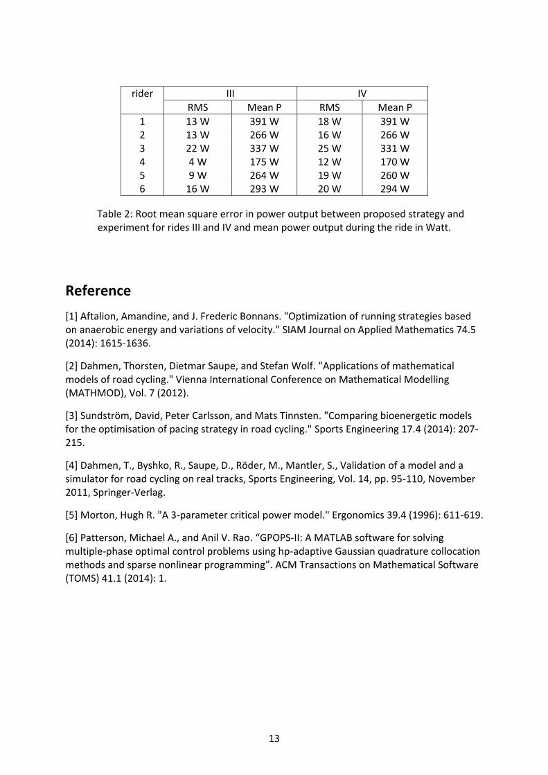
rider III IV

RMS Mean P RMS Mean P

1 13 W 391 W 18 W 391 W 2 13 W 266 W 16 W 266 W 3 22 W 337 W 25 W 331 W 4 4 W 175 W 12 W 170 W 5 9 W 264 W 19 W 260 W 6 16 W 293 W 20 W 294 W

Table 2: Root mean square error in power output between proposed strategy and experiment for rides III and IV and mean power output during the ride in Watt.

Reference

[1] Aftalion, Amandine, and J. Frederic Bonnans. "Optimization of running strategies based on anaerobic energy and variations of velocity." SIAM Journal on Applied Mathematics 74.5 (2014): 1615-1636.

[2] Dahmen, Thorsten, Dietmar Saupe, and Stefan Wolf. "Applications of mathematical models of road cycling." Vienna International Conference on Mathematical Modelling (MATHMOD), Vol. 7 (2012).

[3] Sundström, David, Peter Carlsson, and Mats Tinnsten. "Comparing bioenergetic models for the optimisation of pacing strategy in road cycling." Sports Engineering 17.4 (2014): 207-215.

[4] Dahmen, T., Byshko, R., Saupe, D., Röder, M., Mantler, S., Validation of a model and a simulator for road cycling on real tracks, Sports Engineering, Vol. 14, pp. 95-110, November 2011, Springer-Verlag.

[5] Morton, Hugh R. "A 3-parameter critical power model." Ergonomics 39.4 (1996): 611-619.

[6] Patterson, Michael A., and Anil V. Rao. “GPOPS-II: A MATLAB software for solving multiple-phase optimal control problems using hp-adaptive Gaussian quadrature collocation methods and sparse nonlinear programming”. ACM Transactions on Mathematical Software (TOMS) 41.1 (2014): 1.

13

Two Body Dynamic Model for Speed Skating Driven by the Skaters Leg Extension

E. van der Kruk, H.E.J. Veeger , F.C.T. van der Helm and A.L. Schwab

Department of Biomechanical Engineering, Delft University of Technology, Mekelweg 2, Delft, the

Netherlands, e.vanderkruk@tudelft.nl

Introduction

In speed skating forces are generated by pushing in a sideward direction against an environment, which moves relative to the skater. De Koning et al. (1987) showed that there is a distinct difference in the coordination pattern between (elite) speed skaters. Models can help to give insight in this peculiar technique and ideally find an optimal motion pattern for each individual speed skater. Currently there are three models describing and optimizing the behaviour and performance of skaters, of which only two are relevant in terms of coordination patterns (Allinger & Bogert, 1997; Otten, 2003). However, none of them have been shown to accurately predict the observed coordination pattern via verification with empirical kinetic and kinematic data. Therefore, the objectives of this study are to present a verified three dimensional inverse skater model with minimal complexity, based on the idea of (Cabrera, Ruina, & Kleshnev, 2006), modelling the speed skating motion on the straights. The model is driven by the changing distance between the torso and the skate (further referred to as the leg extension), which is also the true input of the skater to generate a global motion. This input, which is indirectly also a measure of the knee extension of the skater, is a variable familiar to the speed skaters and coaches. In this extended abstract we verify this novel model for two strokes (left and right) of one skater through correlation with observed kinematics and forces.

METHODS

2.1 Model Description

The model presented in this section simulates the upper body transverse translation of the skater together with the forces exerted by the skates on the ice. The model input is the measured leg extension (coordination pattern). Based on empirical data from previous studies using elite skaters, the double stance phase, the time in which both skates are in contact with the ice, is rather short. For the sake of simplicity, we assume that there is only one skate at a time in contact with the ice, alternating left and right. The point of alternation is defined as the moment in time where the forces exerted on both skates are equal.

14

Furthermore the arm movements and the rotations of the upper body are assumed to be of marginal effect on the overall power and are therefore neglected. Based on these assumptions, the skater can be considered as a combination of two point masses, which are situated at the upper body (mass B) and at each (active) skate (mass S). The body mass of the skater is distributed over the two active masses by a constant mass distribution coefficient (η) to compensate for the shift in the center of mass position during the speed skating movement. Each mass has three degrees of freedom. The set of parameters is

restricted to the position coordinates of mass B ( , ,b b bx y z ), two translations in the transverse

plane of mass S with the position coordinates ( ,s sx y ) (because the skate is assumed to be on

the ice, making zs=0 at all times) and one rotation in the same plane, the steer angle (φS). The orientation of the skate is of importance for the constraint forces acting on the skate. All other rotations of the skates are ignored.

Since we want to obtain a model which is driven by generalized (local) coordinates, we

introduce a set of generalized coordinates iq (Figure 1), so the global coordinates can be

expressed in terms of leg extension via the kinematic relation ( )i ix f q . These generalized

coordinates consist of the leg extension ( , , ,s s s sw u v )(Figure 1), that is actively controlled by

the skater and therefore serves as the input coordinates to the model and the generalized

coordinates of the upper body ( ,b bu v ), which will be a result of the system dynamics (equal

to ,b bx y )

The equations of motion are expressed in generalized coordinates, so that the constraints are inherently fulfilled. Since we assume no lateral slip, a non-holonomic constraint acting in the lateral direction of the skate was added, causing the undetermined external force λ perpendicular to the skate blade in the transverse plane. This leaves a model with two degrees of freedom in position and only one in velocity. The known external forces acting on the model are the air frictional forces and the ice frictional forces.

2.2 Solving the Model

The model is solved in two steps. First, since the parameters ( , , ,s s s sw u v ) are considered

inputs and the air frictional forces acting on the upper body are assumed to be known, the

constraint force λ and the transverse position of the upper body ( ,b bu v ) can be determined

by means of integration (Runge Kutta method), starting from the initial condition

,0 ,0 ,0 ,0, , ,b b b bx y x y. The constraint is fulfilled for each integration step by a projection

method. Hereby a minimization problem was formulated, concerning the distance from the predicted solution to the solution which is on the constraint surface. The global coordinates

ix , which are the global positions of the upper body and the skate, can then be found

analytically via the kinematic relation. Finally, with the found upper body position and ,

the local forces acting on the skate can be solved analytically such that a complete two-body dynamic model of the skater has been established.

15

2.3 Model Verification

The purpose of the model verification is to quantify the error between the simulated data and the measured forces and positions. The forces were measured by a set of instrumented klapskates (van der Kruk, den Braver, Schwab, van der Helm, & Veeger, 2016). The position of the masses was measured by a motion capture system on 50 meter of the straight part of the rink, with a passive marker on the Lateral Malleolus (representing mass S) and on the back near the Sacrum (representing mass B). A parametric function was fitted to the recorded data, consisting of a linear and a geometric function, which could be differentiated twice in order to obtain velocity and acceleration data. The air and ice friction were estimated based on previous papers (J. J. De Koning, De Groot, & Van Ingen Schenau, 1992; van Ingen Schenau, 1982). The body mass was assumed to be distributed equally over mass S and mass B. In this abstract the data of one Dutch elite female speed skater are presented (65kg, 1.75m).

Figure 1: The global and generalized coordinates of the two-mass skater model. Leg extension consists of vertical distance (ws) and horizontal distance between the mass S and mass B in heading direction (us) and perpendicular to heading direction

(vs) and the heading of the skate (θs) (orientation).

16

Figure 2 The measured (Qualisys), fitted and modelled data of two consecutive strokes for position and velocity of mass B and the total force. The grey area indicates a left stroke, the white area a right stroke, the pattern indicates the double stance phase as measured.. Y

is in line with the skate lane, X is perpendicular to the skate lane.

RESULTS

The results show that the model estimated the forward position and velocity of mass B the best (Jmin (based on (Cabrera et al., 2006))), followed by the lateral position and velocity, which were all within 1% accuracy. The model was least accurate for the force determination (Table 1). The forces were consistently estimated too low (Figure 2, bottom graph).

17

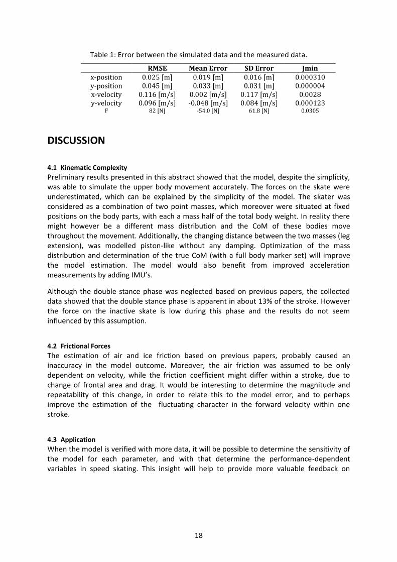
DISCUSSION

4.1 Kinematic Complexity

Preliminary results presented in this abstract showed that the model, despite the simplicity, was able to simulate the upper body movement accurately. The forces on the skate were underestimated, which can be explained by the simplicity of the model. The skater was considered as a combination of two point masses, which moreover were situated at fixed positions on the body parts, with each a mass half of the total body weight. In reality there might however be a different mass distribution and the CoM of these bodies move throughout the movement. Additionally, the changing distance between the two masses (leg extension), was modelled piston-like without any damping. Optimization of the mass distribution and determination of the true CoM (with a full body marker set) will improve the model estimation. The model would also benefit from improved acceleration measurements by adding IMU’s.

Although the double stance phase was neglected based on previous papers, the collected data showed that the double stance phase is apparent in about 13% of the stroke. However the force on the inactive skate is low during this phase and the results do not seem influenced by this assumption.

4.2 Frictional Forces

The estimation of air and ice friction based on previous papers, probably caused an inaccuracy in the model outcome. Moreover, the air friction was assumed to be only dependent on velocity, while the friction coefficient might differ within a stroke, due to change of frontal area and drag. It would be interesting to determine the magnitude and repeatability of this change, in order to relate this to the model error, and to perhaps improve the estimation of the fluctuating character in the forward velocity within one stroke.

4.3 Application

When the model is verified with more data, it will be possible to determine the sensitivity of the model for each parameter, and with that determine the performance-dependent variables in speed skating. This insight will help to provide more valuable feedback on

Table 1: Error between the simulated data and the measured data.

RMSE Mean Error SD Error Jmin x-position 0.025 [m] 0.019 [m] 0.016 [m] 0.000310 y-position 0.045 [m] 0.033 [m] 0.031 [m] 0.000004 x-velocity 0.116 [m/s] 0.002 [m/s] 0.117 [m/s] 0.0028 y-velocity 0.096 [m/s] -0.048 [m/s] 0.084 [m/s] 0.000123

F 82 [N] -54.0 [N] 61.8 [N] 0.0305

18

technique to skaters and coaches and via optimization propose individual optimal coordination patterns.

References Allinger, T. L., & Bogert, A. J. (1997). Skating technique for the straights based on the

optimization of a simulation study. Medicine and Science in Sports and Exercise, 29, 279–286.

Cabrera, D., Ruina, a., & Kleshnev, V. (2006). A simple 1+ dimensional model of rowing mimics observed forces and motions. Human Movement Science, 25(2), 192–220. http://doi.org/10.1016/j.humov.2005.11.002

de Koning, J. J., de Boer, R. W., de Groot, G., & van Ingen Schenau, G. J. (1987). Push-Off Force in Speed Skating, 103–109.

De Koning, J. J., De Groot, G., & Van Ingen Schenau, G. J. (1992). Ice friction during speed skating. Journal of Biomechanics, 25(6), 565–571. http://doi.org/10.1016/0021-9290(92)90099-M

Otten, E. (2003). Inverse and forward dynamics: models of multi-body systems. Phil. Trans. R. Soc. Lond., 1493–1500.

van der Kruk, E., den Braver, O., Schwab, A. L., van der Helm, F. C. T., & Veeger, H. E. J. (2016). Wireless instrumented klapskates for long-track speed skating. Journal of Sports Engineering. http://doi.org/10.1007/s12283-016-0208-8

van Ingen Schenau, G. J. (1982). The influence of air friction in speed skating. Journal of Biomechanics, 15(6), 449–458. http://doi.org/10.1016/0021-9290(82)90081-1

19

Predicting maximum speed in a 4x1000 m Field Test based on estimated VO2max values from Shuttle

Run Test and Queens College Step Test

Jörg M. Jäger1, Johannes Kurz2 and Hermann Müller3

1Institute of Sport Science, Justus-Liebig-University Gießen, joerg.jaeger@sport.uni-giessen.de

2Institute of Sport Science, Justus-Liebig-University Gießen, johannes.kurz@sport.uni-giessen.de

3Institute of Sport Science, Justus-Liebig-University Gießen, hermann.mueller@sport.uni-giessen.de

Introduction

The maximal oxygen uptake (VO2max) measures the maximum amount of oxygen that an individual can use per unit of time during strenuous physical exertion. It is one of the most distinguished measures in endurance sports and serves as an index of cardiorespiratory function, general health, and aerobic fitness [1]. Besides its physiological meaning, VO2max is also relevant in exercise prescription. The intensity of cardiorespiratory exercise [2] and endurance training is commonly quantified as a percentage of VO2max. Due to that, assessing the maximal oxygen uptake plays an important role in endurance sport. It provides a basis for diagnosing aerobic capacity or designing programs to improve cardiovascular fitness. Since VO2max is also one of the predominant limiting factors in endurance exercises and training, it may also serve as a predictor for performance in endurance sports

This study aims to (a) estimate the VO2max in healthy adults by two common endurance tests and (b) construct and evaluate a statistical model that predicts the performance in a 4x1000 m Field Test based on these estimated VO2max values.

Methods

29 subjects participated in this study (8 male: age 28.8 ± 8.4 years, height 186.4 ± 5.7 cm, mass 81.4 ± 8.7 kg, and 21 female: age 22.8 ± 2.6 years, height 169.0 ± 6.9 cm, mass 59.8 ± 6.6 kg). Each subject gave written consent to participate in the following three tests:

(1) The Shuttle Run Test (SRT)(e.g. [3], [4]): Subjects ran shuttles between two marked lines placed 20 m apart at increasing fast speeds. Running speed was increased each minute from one level to another. Accordingly, each level consisted of a different number of shuttles within that minute (from 7 runs in level 1 up to 16 runs in level 21). Subjects were verbally

20

encouraged to give maximum effort in this test. VO2max of subjects were determined based on their successfully completed levels and runs (see [4]).

(2) The Queens College Step Test (QCST)[5]: The test started with a 3 min rest when the subjects sat on a bench step (height: 41 cm). For women, a metronome was set at 88 beats per minute (bpm) leading to 22 steps per minute, for men it was set at 96 bpm leading to 24 steps per minute. Subjects made contact with a foot on each beep of the metronome in an up-up-down-down manner. After exactly 3 min of stepping, the subjects stopped and palpated for the radial pulse at exactly 3:05 to 3:20. Recovery heart rate (HR) was derived for a full minute (bpm) and used to calculate VO2max based on the following formulas from [5]:

Men: VO2max [ml∙kg−1 ∙min−1] = 111.33 - (0.42 × HR), Women: VO2max [ml∙kg−1 ∙min−1] = 65.81 - (0.1847 × HR))

(3) The 4x1000 m Field Test (FT)[6]: In this test, the subjects individually chose their running speed based on written instructions. The first three runs requested incremental running speeds corresponding to common training intensities (slow, medium and fast). The last run corresponded to the maximum speed that the subjects can run for a 1000 m. Therefore, the term maximum speed refers to the average speed achieved and maintained in the last maximal effort trial of the 4x1000-m-Field-Test. Between each run a two-minute rest was allowed. Instructions for runs defined the different intensities according to (a) the usual durations of such runs, (b) a rating of perceived exertion after these runs, and (c) information about the breathing during the runs (e.g. “slow” refers to an intensity of a 1 h jog which is a bit tiring but not exhausting, where breathing and talking is easy). Participants were also instructed to run a preferably constant pace in each trial [cf. 7].

The SRT (1) and QCST (2) were chosen, because they estimated the subjects’ VO2max from

different points of view. Test (1) is a maximal effort test that aims at an athlete’s ability to continue an incremental endurance activity and primarily resist to fatigue. In contrast, test (2) is a submaximal effort test which measures the recovery heart rate of an athlete, because it returns to resting values more quickly in fitter people than it does in those who are less fit.

The VO2max estimates from test (1) and (2) were used in a multiple regression model as predictor variables (SRTVO2max from Shuttle Run Test and QCSTVO2max from Queens College Step Test). In that regression model, maximum speed in a 1000 m run (in FT) served as the criterion variable (i.e. the outcome).

Results

Estimated VO2max values for males were 49.3 ± 5.3 [ml∙kg−1 ∙min−1] in SRT and 55.3 ± 9.8 [ml∙kg−1 ∙min−1] in QCST. For female they were 41.9 ± 5.5 [ml∙kg−1 ∙min−1] in SRT and 40.3 ± 3.6 [ml∙kg−1 ∙min−1] in QCST. Figure 1 shows a grouped boxplot of the results according to the two tests.

The VO2max values from SRT and QCST were significantly correlated (r = 0.72, p < 0.01). An ANOVA (factor group with two levels: male and female; factor test with two levels: SRT and

QCST) revealed a significant main effect of group (F(1, 27) = 28.46, p < 0.01, 2 = 0.45), i.e. men had higher VO2max values than women, but no main effect between the both tests (F(1,27) = 0.22, p = 0.64). Thus, the two tests did not differ systematically, i.e. they did not

21

show significant differences in estimating the subjects’ oxygen uptake. However, we found a

significant interaction effect (F(1,27) = 12.09, p < 0.01, 2 = 0.09), i.e. men tended to achieve higher scores in QCST compared to SRT, while the scores for women were not influenced. However, effect size of this interaction was quite small.

Figure 1. Boxplot of estimated VO2max for male and female participants based on Shuttle-Run-Test (SRT) and Queens-College-Step-Test (QCST)

Multiple regression analysis was used to test if the estimated VO2max from SRT and QCST significantly predicted participants' maximum speed. The mean across participants of the maximum speeds in the 1000 m runs was 15.1 ± 1.5 km/h for men and 13.2 ± 1.4 km/h for women. The results of the regression model indicated the two predictors explained 65% of the variance (R2

ad = 0.65, F(2,26) = 26.46, p < 0.01). Furthermore, the prediction of the model was evaluated by a 10-fold-cross-validation approach. An overall root mean square error (RMSE) of 1.03 km/h was obtained.

Conclusions

The estimated VO2max from both the Shuttle Run Test and the Queens College Step Test are, taken all together, able to predict a remarkable amount (65%) of variance in maximum speed in a 1000 m run. This is in line with the concept that VO2max has an important influence on endurance performance.

A mean prediction error of approximately 1 km/h of the real maximum speed seems to be small, but may still be too big to allow detailed recommendations for training based on

40

50

60

70

male female

VO

2m

ax (

ml / kg

/ m

in)

TestSRT

QCST

22

running velocities. Additionally, there is still 35% variance left that could not be explained by this statistical model. Many aspects may have contributed to this unexplained variance. For instance, the motivation of the subjects in maximal effort tests (such as the SRT and the last trial in FT) and environmental factors could have influenced the results profoundly. With respect to environmental factors, the tests were performed on varying floor types and different days and therefore with varying weather conditions. Other aspects may be related to the different facets of endurance. The 4x1000 m Field Test requires resistance to fatigue (in each run) as well as a quick recovery (in between to runs). Thus, a specific combination of these two aspects is important for this test and affects the maximum speed in the last 1000 m run. The SRT and the QCST, however, focus mainly on one of these aspects rather than the combination of both. Last but not least, the athletes’ anaerobic energetics might have an impact, too. In a short duration 1000 m run, anaerobic metabolism contributes substantially to the total energy expenditure. Therefore, variations in the anaerobic energetics between runners might also contribute to the observed variance in running speed. Taken together, these aspects may limit the prediction and amount of explained variance based on their estimated VO2max values.

Furthermore, even though the estimated VO2max values from SRT and QCST were highly correlated, both tests did not measure oxygen uptake directly with a spirometer. Although the SRT was validated with respect to estimating VO2max, we still have to consider an estimation error. For instance [8] found a standard error of estimate of 5.4 [ml∙kg−1 ∙min−1] in an early version of the SRT. This applies analogously to the inaccuracy of the QCST results. While formulas from [5] appear to be very accurate, [9] found a standard error of prediction of 2.9 [ml∙kg−1 ∙min−1] in their test persons. Hence, the two predictor variables in our linear model may be inaccurate to a certain amount, which also affects the accuracy in predicting the speed as outcome variable.

To finalize, the multiple regression approach in this study also neglects other potential predictors like age, sex, as well as further experiences with endurance sports, and – from a methodological point of view – the regression is statistically based on linear models. This, however, may be a severe limitation, because in real world settings many influencing factors and non-linear processes occur in contexts of sports.

A next step should be to improve the prediction model by adding further variables that might influence and explain performance in a 1000 m run. Besides that, different non-linear alternatives for modeling also seem to be promising to improve the accuracy of the prediction. Artificial neural networks, particularly multilayer perceptrons, may provide more sophisticated non-linear approaches for prediction. However, a major amount of variance in maximum speed can already be explained from the linear model approach chosen in this study.

Reference

[1] Deuster, P.A. & Heled, Y. (2008). Testing for maximal aerobic power. In Seidenberg, P. H. and Beutler, A. I. (Eds.), The sports medicine resource manual (pp. 520-528). Philadelphia, PA: Elsevier.

23

[2] ACSM (2011). Quantity and quality of exercise for developing and maintaining cardiorespiratory, musculoskeletal, and neuromotor fitness in apparently healthy adults: Guidance for prescribing exercise. Medicine & science in sports & exercise, 43(7), 1334-1359.

[3] Léger, L.A., Mercier, D., Gadoury, C., & Lambert, J. (1988). The multistage 20 metre shuttle run test for aerobic fitness. Journal of sports sciences, 6, 93-101.

[4] Ramsbottom, R., Brewer, J., & Williams, C. (1988). A progressive shuttle run test to estimate maximal oxygen uptake. British journal of sports medicine, 22(4), 141-144.

[5] Haff, G. G., & Dumke, C. (2012). Laboratory Manual for Exercise Physiology. Champaign, IL: Human Kinetics.

[6] Held, T. (2000). Überprüfung der Ausdauerleistungsfähigkeit. Der 4x1000-m-Lauftest (mobilepraxis) [Assessing endurance performance. The 4x1000-m-Test]. mobile - Die Fachzeitschrift für Sport, 6, 5-9.

[7] Held, T., Steiner, R., Hübner, K., Tschopp, M., Peltola, K., & Marti, B. (2000) . Selbst gewählte submaximale Laufgeschwindigkeiten als Prädiktoren des Dauerleistungsver-mögens [Self-selected submaximal running velocities as predictors of endurance capacity]. Schweizerische Zeitschrift für Sportmedizin und Sporttraumatologie, 48(2), 64-69.

[8] Léger, L.A., & Lambert, J. (1982). A maximal multistage 20-m shuttle run test to Predict VO2max. European journal of applied physiology, 49, 1-12.

[9] McArdle, W. D., Katch, F. I., Pechar, G. S., Jacobson, L., & Ruck, S. (1972). Reliability and interrelationships between maximal oxygen intake, physical work capacity and step-test scores in college women. Medicine & science in sports & exercise, 4(4), 182-186.

24

Determination of Critical Speed and the Running Distance above Critical Speed under Laboratory and

Field Conditions using Equal Exhaustive Durations – a Pilot Study

Christoph Triska1, Bettina Karsten2, Harald Tschan1, and Alfred Nimmerichter3

1University of Vienna, Centre for Sport Science and University Sports, Institute of Sport Science,

christoph.triska@univie.ac.at

2University of Greenwich, Department of Life and Sports Science, kb20@gre.ac.uk

3Univeristy of Applied Sciences Wr. Neustadt, Sport and Exercise Sciences, nimmerichter@fhwn.ac.at

Introduction

The power-duration concept of Critical Power (CP) [1] and its related ‘anaerobic’ parameter (W´) was adapted to treadmill running in the early 1980ies by Hughson et al. [2] and consequently termed Critical Speed (CS) and its ‘anaerobic’ parameter Running Distance Above CS (D´). This finite distance can be maximally run, when performing at values above CS.

Today, coaches and sport scientists use this concept to assess performance, to prescribe training, and to predict performance. Traditionally, these tests were carried out only under laboratory conditions. However, field tests are preferred over laboratory test by many coaches due to their similarity to competitive races and their reflection of real-world training. Field tests carry a higher level of ecological validity, although lack of environmental control is often criticized. To translate relevant laboratory tests into the field arguably presents a challenge for sport scientists.

Previous work

A growing body of literature has assessed the interchangeable use of CS and CP under laboratory and field conditions.

For example, Galbraith et al. [3] postulated that the determination of CS can be translated into field conditions as their work did not find a significant differences between respective CS values. However, these authors demonstrated significant differences in D´ between conditions. Recently, another study assessing CS and D´ under both conditions found significant differences for both, CS and D´ [4].

25

Similar to running, studies have compared estimates of CP and W´ between laboratory and field conditions [5-7]. These results demonstrated non-significant differences and a good level of agreement for CP, but not for W´.

Aforementioned studies [3-6] used different durations for the prediction trials under laboratory and field conditions and these differences in duration might explain the significant differences in W´/D´. When comparing time-to-exhaustion runs under laboratory conditions with time-trials or fixed distances under field conditions, it seems obvious that it is nearly impossible to match the exact duration of the corresponding prediction trial.

Therefore, the aim of this study was to evaluate CS and D´ between treadmill running and over-ground running using equal durations for the corresponding prediction trial. A recent study suggested to use equal duration of the prediction trials to alleviate differences in D´ [4]. We hypothesized non-significant differences and a good agreement between laboratory and field estimates CS and D´.

Methods

Six moderately trained soccer players (mean ± SD: age 25.6 ± 2.5 yrs; stature 179.3 ± 5.4

cm; body mass 73.8 ± 7.0 kg; ��O2max 53.8 ± 3.1 mL∙min-1∙kg-1) volunteered to participate in this study. Participants had to give written informed consent after all experimental procedures were explained. The study was conducted in accordance to the declaration of Helsinki and all procedures have been approved by the local ethics committee (Ref. nbr. 00155).

After an initial incremental exercise test to determine respiratory thresholds and maximum aerobic speed (MAS), participants performed three prediction trials leading to exhaustion on a treadmill and on a 400 m athletics track. Speeds for the laboratory test were taken as 75%Δ of the difference between speed at first respiratory threshold and MAS, 98% of MAS (i.e. 0.98 x MAS) and 108% of MAS (i.e. 1.08 x MAS). These intensities have shown to lead to exhaustion between 2.5 and 15 min [4, 5]. Treadmill grade was set to 1% to compensate for air resistance. Under field conditions, participants were asked to cover the greatest distance possible within the time achieved during the respective prediction trial. All prediction trials were interspersed with 30 min passive rest [3-6]. The parameter estimates (CS and D´) were resolved using the linear speed/inverse-time model:

𝑠𝑝𝑒𝑒𝑑 = 𝐷´ 𝑥 1/𝑡 + 𝐶𝑆 (1)

where speed is in m∙s-1, and t represents time (s).

Results

Using the Shapiro-Wilk test all data was normally distributed. A paired sample t-test revealed no significant differences between the conditions (P = 0.548 and P = 0.265 for CS and D´, respectively). Results of the tests are presented in Table 1. Moreover, we found significant correlations between the conditions (r = 0.947; P = 0.004 and r = 0.913 and P = 0.011 for CS and D´, respectively) (Figure 1). The bias was 0.04 ± 0.13 m∙s-1 (95% LoA: -0.23 to 0.30 m∙s-1) for CS and -17.3 ± 33.8 m (95% LoA -83.5 to 48.9 m) for D´ (Figure 2).

26

Conclusions

The main finding of this study was that when using equal exhaustive durations non-significant differences between the conditions were observed for both, CS and D´.

Our results for CS are supported by previous findings [3, 5], but results for D´ are in vast contrast to previous works [3-7]. A significant correlation was shown only for CS between the conditions in previous works [3-7], and only a single study found a significant correlation for D´ between the conditions [5]. In comparison to previous studies we found higher correlation coefficients for CS and D´ (r > 0.913) and significant correlations (P < 0.011) compared to studies using non-equal durations [3-5]. The 95% Limits of Agreement (LoA) revealed a closer agreement between methods compared to other studies assessing CS (0.04 m∙s-1 vs. 0.25 m∙s-1

[3] and -0.39 m∙s-1 [4]) and D´ (-17.3 m vs. 187 m [3] and 36.7 m [4]).

This is the first study that found a non-significant difference, a close agreement, and a significant correlation between the conditions for CS and for D´. Using equal durations under both conditions therefore represent a valid comparison for CS and D´. Our results support the use of both test interchangeably. CS and D´ are considered a valid measure under both conditions.

Laboratory Field conditions

CS (m∙s-1) 3.87 ± 0.39 3.84 ± 0.41 D´ (m) 225.1 ± 80.5 242.5 ± 81.2

Table 1: Results of the CS (m∙s-1) and D´(m) tested under laboratory and field conditions.

Figure 1: (a) Relationship between CS during laboratory and field test. (b) Relationship between D´ during laboratory and field test. Solid line represents the line of identity.

27

Figure 2: Bland-Altman plot of the difference in (a) CS (b) and D´ during the laboratory and field test.

Reference

[1] H. Monod and J. Scherrer, "The work capacity of a synergic muscular group," Ergonomics, vol. 8, pp. 329-338, 1965.

[2] R. L. Hughson, C. J. Orok, and L. E. Staudt, "A high velocity treadmill running test to assess endurance running potential," Int J Sports Med, vol. 5, pp. 23-5, Feb 1984.

[3] A. Galbraith, J. Hopker, S. Lelliott, L. Diddams, and L. Passfield, "A single-visit field test of critical speed," Int J Sports Physiol Perform, vol. 9, pp. 931-5, Nov 2014.

[4] C. Triska, B. Karsten, G. Tazreiter, H. Tschan, and A. Nimmerichter, "Comparison of Single-Visit Critical Speed Testing Protocols under Laboratory and Field Conditions," under review, 2016.

[5] C. Triska, H. Tschan, G. Tazreiter, and A. Nimmerichter, "Critical Power in Laboratory and Field Conditions Using Single-visit Maximal Effort Trials," Int J Sports Med, vol. 36, pp. 1063-8, Nov 2015.

[6] B. Karsten, S. A. Jobson, J. Hopker, L. Stevens, and C. Beedie, "Validity and reliability of critical power field testing," Eur J Appl Physiol, vol. 115, pp. 197-204, Jan 2015.

[7] B. Karsten, S. A. Jobson, J. Hopker, A. Jimenez, and C. Beedie, "High agreement between laboratory and field estimates of critical power in cycling," Int J Sports Med, vol. 35, pp. 298-303, Apr 2014.

28

Ball (not) in play: the distortive effect of net playing time on the decline of match running performance in

professional football

Daniel Linke, Martin Lames

Technical University Munich, Department for Training and Computer Science in Sports,

Georg-Brauchle-Ring 60/62, Munich, Germany, daniel.linke@tum.de

Introduction

This study aimed to (1) compare established running performance parameters in respect to the development of fatigue and (2) determine whether the frequently reported declines in physical performance are distorted by an increase of game stoppages towards the end of a football game.

Methods

1134 individual match performances from eighty-one German Bundesliga games were analyzed during the 2012-2013 and 2013-2014 competitive season, using a multi-camera computerized tracking system (TRACAB, Stockholm, Sweden). Parameters selected for analysis included the relativized distances traveled in generally used speed zones, number of accelerations and sprints as well as metabolic power. Performance data were divided into eighteen 5min periods for the analysis of temporal changes over the course of the game. Student’s t-test and ANOVA with Bonferroni post hoc tests were used to identify effect sizes of temporal changes considering both absolute and actual playing time (excluding game interruptions).

Players’ running performances were divided into the following categories: total distance (TD), walking (0.7-7.2 km • h-1), jogging (7.2-14.4 km • h-1), running (14.4-19.8 km • h-1), high-speed running (HSR) (19.8-25.2 km • h-1), and sprinting (> 25.2 km • h-1). High intensity running (HIR) consisted of running, high-speed running, and sprinting. Very high-intensity running (VHIR) consisted of high-speed running and sprinting. We further subdivided the distances covered at low, moderate and high acceleration (LACC, 0-2 m • s-2; MACC, 2-3 m • s-2; HACC, >3 m • s-2) and deceleration (LDEC, 0 to -2 m • s-2; MDEC, -2 to -3 m • s-2; HDEC, < -3 m • s-2).

Acceleration and deceleration efforts were classified as consecutive samples (0.2 s) exceeding the abovementioned acceleration and deceleration thresholds (#LACC, #MACC, #HACC, #LDEC, #MDEC, #HDEC. A sprint was defined as the attainment of sprint speed (> 25.2 km • h-1) for a minimum of 0.5 s.

29

Finally, the metabolic power equations were also included in the analysis in order to estimate the average metabolic power (PMET, W • kg-1) at any given moment.

All categories were relativized to a minute by minute value.

Results

Initially we found a significant decline in effective playing time (Et, p < .01) over the course of a match, accounting for a decrease from 69% of the total play time in the 1-5min period to 56% in the 85-90min period. In consideration of the total playing time (Tt), performance parameters decreased by 26.2% on average (η² = 0.29, corresponding to large effect sizes). Considering the effective playing time (Et), performance parameters decreased by only 12.1% on average (η² = 0.12, corresponding to medium effect sizes) (Figure 1).

Figure 1: Changes in match running performance between the first (0-5min) and last (85-90min) match period; left figure shows the average percentage change of the different movement categories; right figure

shows the resulting effect sizes d of the observed differences; comparison between effective playing time (Et) and total playing time (Tt)

Conclusions

In conclusion, this study showed that the decrease in physical performance during a football match is strongly enhanced by an increase of game interruptions over the course of the game. This indicates that the occurring fatigue in professional football should be examined in consideration of the actual playing time.

30

Prediction of individual short term heart rate responses

Katrin Hoffmann1

1Institute of Sports Science, Technische Universität Darmstadt, Hoffmann@sport.tu-darmstadt.de

Introduction

In the physical training process, optimal training adaptations require individually optimal strain on the human body. Especially in endurance training, the individual heart rate (HR in beats per minute) response has become a very important indicator to measure and determine the individual strain. As the same load can lead to complete different responses in different individuals the prediction of this individual HR response is very challenging and one of the key problems in the physical training process. This paper is analyzing two different procedures to predict individual HR responses for cycling on a bike ergometer.

Methods

HR data of sixteen healthy and physically active participants were recorded and processed while the participants were playing the Exergame “LetterBird” [1]. This game was developed by the communication laboratory in Darmstadt and aimed at realizing playful endurance training.

All tests were performed on a Daum Cycle Ergometer (8008 TRS 3) with a flywheel. HR was constantly monitored by a chest belt (POLAR, T31), processed by the ergometer and logged together with the corresponding time stamp (in milliseconds), with the Power in W (measured by the ergometer) and the pedal rate (PR) in revolutions or rates per minute (rpm; measured at the flywheel). The PR controlling the game was expected to have no influence on the HR [2]. The individual optimal training range was set to 70 – 80% of the maximal HR (HRmax) depending on age (in years) calculated with the formula:

𝐻𝑅𝑚𝑎𝑥 = 220 − 𝑎𝑔𝑒 [3] The first procedure was developed basing on literature research [4] and aimed at

calculating the individual HR response using a calibration phase prior to the actual training phase. Therefore, the individual HR responses to two defined load levels set at the ergometer were measured. Depending on the body weight and the BMI of the participants these successive load levels were set at the ergometer for 2 minutes each. Expecting a linear relationship of load and HR response in submaximal range an algorithm calculating load that is expecting to evoke a defined HR was developed. Using the HR data obtained the algorithm calculated the load that was expected to evoke an individually optimal training HR of 75 % HRmax. After a break the calibration phase was replicated to validate the results, successively followed by one minute of the calculated target load and another five minutes of an automatic

31

load control (ALC). In the ALC the load automatically adapts the load if the HR exceeds or falls below the training range.

The second procedure aimed at predicting the individual HR response to the change of load bouts while training or cycling. Therefore, the HR data obtained with procedure 1 were approximated using the formula

𝐻𝑅 = 𝐻𝑅𝑒𝑛𝑑 – (𝐻𝑅𝑒𝑛𝑑 – 𝐻𝑅𝑠𝑡𝑎𝑟𝑡) ∗ 𝑒 –𝑐∗𝑡 [5] with value c representing the slope of the HR course. First, reliability of the approximated

data was calculated. In a second step, the c values representing the slope of the course of the two load levels of the calibration phase were analyzed. As the changes of load bouts were similar in both load levels we tested the hypotheses that the c values were also similar using the Wilcoxon-Test. In the third test, HR data at discrete time points (10 sec (t1), 20 sec (t2), 30 sec (t3), 40 sec (t4), 50 sec (t5), 60 sec (t6) and 90 sec (t7)) and parameter c of the first load level was used to predict the final HR of the second load using the formula

𝐻𝑅𝑒𝑛𝑑−𝑐𝑎𝑙𝑐 = 𝐻𝑅 − 𝐻𝑅𝑠𝑡𝑎𝑟𝑡 ∗ 𝑒−𝑐∗𝑡

1 − 𝑒−𝑐∗𝑡

The deviation of the calculated HR end and the measured HR end was calculated and analyzed using Wilcoxon. Cronbach´s Alpha was calculated for reliability over all time points.

Results

Using procedure 1, fifteen of sixteen participants reached the final HR zone in the exercise phase within 10 min (deviation of measured and expected HR between 9:30 – 10:00 after onset of exercise; M = 3.98 bpm; SD = 3.12; Range = 11.61 bpm). One participant exceeded the training range with 80.6% HRmax. In the ALC, the load was adapted downwards in 13 of 16 participants.

The regression analysis using procedure 2 revealed a regression coefficient R² of 0.864 (SD = 0.126, Range = 0.210)

Parameter c of load level 1 is not significantly different to parameter c of load level 2 (Δ c1 – c2: M = 0.02, SD = 0.37, Range = 1.22, Wilcoxon: z = -0.664, p = 0.507).

The deviation of the calculated and the measured HR differs significantly in time points t1, t2 and t3. There is no significant deviation in time points t4 – t7. The lowest deviation can be found in time point t6. All deviations for the corresponding time points are displayed in table 1.

32

t1 t2 t3 t4 t5 t6 t7

M [S/min] -24.1 -12.5 -7.7 -2.2 0.6 1.4 1.7

SD 18.47 17.20 11.36 11.09 9.21 8.37 6.03

Range [S/min] 76 67 42 49 38 31 27

Wilcoxon

-3.310;

p<.01

-2.467;

p<.05

- 2.510;

p<.05

-1.591

not sign.

-0.31

not sign.

-0.199

not sign.

-1.008

not sign.

Table 1: deviation of calculated HR end and measured HR end at discrete time points (Δ HRend_calc – HRend _real

Cronbach α over all time points was 0.921).

Conclusions

The results confirm that it is possible to evoke the expected submaximal HR within 10 minutes. However, the frequently occurring downward adaptations of load caused by an overpassing HR revealed weaknesses. The calculated load occasionally evokes HR responses that exceed the target range. This miscalculation of the target load can be caused by the delayed HR response to load changes. In that case, the load levels of 2 min were not sufficient for the HR to adapt to the load properly.

The second procedure reveals a possible prediction of the individual HR course already while training within the tested sample. However, a sample time of at least 40 sec is required to obtain sufficient results.

In future research, not only discrete time points but the whole course and slope of the HR response should be integrated in the calculations.

Reference

[1] Hardy S, Göbel S, Gutjahr M, Wiemeyer J, Steinmetz R. (2012). Adaptation Model for Indoor Games. International Journal of Computer Science in Sport; 11 (1):73-85.

[2] Löllgen H., Graham, T., Sjogaard, G. (1980). Muscle metabolites, force, and perceived exertion bicycling at varying pedal rates. Medicine and science in sports and exercise 12(5):345–351.

[3] Robergs, R. A., & Landwehr, R. (2002). The surprising history of the “HRmax= 220-age” equation. J Exerc Physiol, 5(2), 1-10.

[4] Hoffmann K, Wiemeyer J, Hardy S, & Göbel S. (2014). Personalized Adaptive Control of Training Load in Exergames from a Sport-Scientific Perspective. In International Conference on Serious Games. Springer International Publishing, 129-140.

[5] Bunc, V.P., Heller, J. & Leso, J. (1988). Kinetics of heart rate response to exercise. Journal of Sports Science, 6 (1):39-48.

33

A Comparison of Models for Oxygen Consump on

Alexander Ar ga Gonzalez

University of Konstanz, alexander.ar ga-gonzalez@uni-konstanz.de

Introduc onMeasurements of oxygen uptake are central to methods for assessment of physical fitness andendurance capabili es in athletes. Though respiratory gas exchange can easily be measured ina lab, these kind of measurements aren’t prac cable in the field and even less during compe-

ons. Thus, we are looking for a model, which provides the means for fi ng and predic onof oxygen uptake response.Oxygen uptake kine cs are well researched for constant workrate exercises [4] and specificload profiles like ramps [3] or constant work rate, but hardly generalized for variable load pro-files which occur o en in the field. Thus, we compare six dynamic models with power asindependent variable and evaluate their fi ng and predic on abili es.

DataFive healthy, recrea onally to well trained subjects completed four different cycle ergometer(Cylus2, RBM elektronik-automa on GmbH, Leipzig, Germany) tests with con nuous breath-by-breath gas exchange and ven la onmeasurements at themouth (Ergos k, Geratherm Res-piratory GmbH, Bad Kissingen, Germany). The tests were designed to determine a set of usefulphysiological parameters of aerobic capacity (V O2max, ven latory threshold 1 (V T1), and max-imal lactate steady state (MLSS)). Furthermore the tests featured a variety of load profiles inorder to comprehensively evaluate the model predic on quality [1] (Figure 1 and Figure 2).A more detailed describ on of the tes ng procedures and test design can be found in Ar gaGonzalez et al. [1].

Figure 1: Test 1 and Test 2, Subject 2, Physiological Model

34

Figure 2: Test 3 and Test 4, Subject 2, Physiological Model

Models

3.1 Physiological ModelThe first model from Ar ga Gonzalez et al. [1] is based directly on a commonly acceptedmodelfor constant workrate [4] and takes most physiological evidence into account. We extended itby another two parameters to the following:

V O2 = V O2base + x1 (t) + x2 (t)

where x1 (t), x2 (t) are solu ons of

xk (t) = τ−1k (Ak (P (t))− xk (t)) , xk (Tk) = 0, k = 1, 2

with

A1 (P ) = min(s · P, V O2max − V O2base

)A2 (P ) =

{V∆ · exp (− (Pc − P ) /∆) P ≤ PC

V O2max − V O2base − A1 (P ) P > PC

and parameters V O2base, V O2max, PC , s, V∆,∆,τ1, τ2, T1, T2.The physiological model consists of two important parts. The steady-state func on describedby A1 and A2 and the differen al equa ons describing the exponen al behavior. Instead ofchanging the whole model, we can just exchange the steady-state func on and also omit thesecond component. This leads to the following varia ons:

3.1.1 Smooth Steady-State

A smooth alterna ve avoiding the discon nuity at PC :

A1 (P ) = V1max · (1− exp (−s1 · P ))

A2 (P ) =

0 P = 0

V2max ·

(1+tanh

(P2−P2

CP

·s2))

2P > 0

35

3.1.2 Simple Linear Model

Only one linear component: A1 (P ) = min(s · P, V O2max − V O2base

)3.1.3 Simple Exponen al Model

Only one exponen al component: A1 (P ) = V1max · (1− exp (−s1 · P ))

3.2 S rlingThe second model was introduced by S rling et al. [5] and originally designed for running:

V O2(t) = A ·(V O2(t)− V O2min

)B

·(V O2max − V O2(t)

)C

·(D (v, t)− V O2(t)

)E

We adapt it for cycling by replacing the speed based demand func on D (v, t) with a simplelinear demand func on

A (P ) = min(s · P, V O2max − V O2base

). With E = 1 the following parameters are es mated: V O2base, V O2max, s, A, B, C.

3.3 ChengThe third model by Cheng et al. [2] was used for heart rate modeling on a treadmill. As heartrate behaves similar to V O2 (Figure 3), we modified the model for power as input instead oftreadmill speed:

x1(t) = −a1 · x1(t) + a2x2(t) + a6 · P (t)

x2(t) = −a3 · x2(t) +a4 · x1(t)

1 + exp (− (x1(t)− a5))

with x(0) = [x1(0) x2(0)]′ = [0 0]′.

Figure 3: V O2, V CO2and Heart rate measured for one subject during Test 3.

36

Model 3.1 3.1.1 3.1.2 3.1.3 3.2 3.3 3.4 3.5l/min l/min l/min l/min l/min l/min l/min l/min

Subject 1 0.13 0.29 0.20 0.33 0.40 0.38 0.07 0.14Subject 2 0.09 0.12 0.11 0.18 0.24 0.26 0.05 0.10Subject 3 0.06 0.15 0.13 0.21 0.33 0.30 0.07 0.12Subject 4 0.10 0.10 0.07 0.17 0.23 0.21 0.04 0.09Subject 5 0.09 0.11 0.11 0.15 0.26 0.27 0.06 0.08Average 0.09 0.15 0.12 0.21 0.29 0.29 0.06 0.10

Table 1: Average root-mean-square modeling error for all four tests.

3.4 System Iden fica on: Wiener-ModelGoing towards black box models in the field of system iden fica on, the wiener model hasproven well. The wiener model consists of a linear transfer func on followed by a nonlinearfunc on. For these output nonlinearity a piecewise linear func on is selected. This modeltype coincides with the observa on, that there is a linear and a smaller nonlinear rela onshipbetween power and V O2. This can also be seen in Figure 2 and Figure 3.

3.5 Feedforward Neural NetworksAn evenmore recent approach in black boxmodeling are neural networks. Here a feedforwardneural network is taken. The neural networks got trained with randomly resampled data fromTest 3. Different network se ngs from one up to three hidden layers with between 10 and 400neurons were tested.

ResultsAll models were implemented and evaluated in MATLAB®. For parameter es ma on the Ge-ne c Algorithm ga from the Global Op miza on Toolbox™ was used. nlhw and feedforwardnetfrom the System Iden fica on Toolbox™ were used for the Wiener model and the neural net-works.

Table 1 shows the root-mean-square modeling error for all five subjects and all four tests.For predic on, the models were trained on Test 3 and applied on Test 4 (Table 2).

Model 3.1 3.1.1 3.1.2 3.1.3 3.2 3.3 3.4 3.5l/min l/min l/min l/min l/min l/min l/min l/min

Subject 1 0.38 0.38 0.39 0.46 0.49 0.51 0.40 1.51Subject 2 0.31 0.16 0.18 0.21 0.27 0.29 0.21 0.93Subject 3 0.21 0.20 0.23 0.25 0.35 0.52 0.25 1.15Subject 4 0.23 0.18 0.16 0.30 0.29 0.26 0.19 0.86Subject 5 0.38 0.28 0.23 0.23 0.33 0.35 0.29 0.87Average 0.30 0.24 0.23 0.29 0.34 0.39 0.27 1.07

Table 2: Average root-mean-square predic on error for all four tests.

37

The models by S rling and Cheng show weak performance for both, modeling and predic-on. The model by Cheng even turned out unstable for some predic ons.Surprisingly, the smooth varia ons of the physiological model (3.1.1, 3.1.3) performed

worse than their counterparts for modeling.Despite its simplicity, Model 3.1.2 performed well for modeling and predic on. The Physi-

ological Model 3.1 reached a good modeling result but only average for predic on.Be er modeling results are obtained withWiener models which also show someweakness

on predic on.The results of the neural networks are hard to evaluate. If they are trained only once on

the me series from Test 3 than the fi ng error is near zero. We trained them more o en ondifferently sampled data series from Test 3 to avoid overfi ng. Predic on results show, thatthis a empt was not successful. The networks trained once on Test 3 with fi ng errors of 0.00l/min performed similar for predic on.

ConclusionsModeling results below 0.09 l/min are be er than the natural variability in V O2 (unpublishedwork) and they can be regarded as very sa sfactory results. The physiological Model, theWiener models and neural networks are able to perform be er than that threshold.

The best predic onwasmade bymodel 3.1.3 that also s ll fitswell with 0.12 l/min. Overall,the models perform worse than expected for predic on. A reason for that may be, that thedata set is too small and too specific. Most likely, predic on results can be improved by largertraining and valida on data sets.

Also off- and on-transient differences have to be taken into account [6].Another improvement can be obtained by adding further measurements like heart rate as

addi onal input.

References[1] A. Ar ga Gonzalez, R. Bertschinger, F. Brosda, T. Dahmen, P. Thumm, and D. Saupe. Mod-

eling oxygen dynamics under variable work rate. In icSPORTS 2015: 3rd Interna onalCongress on Sport Sciences Research and Technology Support, pages 198–207, 2015.

[2] T. M. Cheng, A. V. Savkin, B. G. Celler, S. W. Su, and L. Wang. Nonlinear modeling andcontrol of human heart rate response during exercise with various work load intensi es.IEEE Transac ons on Biomedical Engineering, 55(11):2499–2508, Nov 2008.

[3] F. Özyener, H. B. Rossiter, S. A. Ward, and B. J. Whipp. Oxygen uptake kine cs duringincremental-and decremental-ramp cycle ergometry. Journal of sports science &medicine,10(3):584, 2011.

[4] D. C. Poole and A. M. Jones. Oxygen uptake kine cs. Comprehensive Physiology, 2:933–996, April 2012.

38

[5] J. S rling, M. Zakynthinaki, and V. Billat. Modeling and analysis of the effect of training onV O2 kine cs and anaerobic capacity. Bulle n of Mathema cal Biology, 70(5):1348–1370,2008.

[6] F. Özyener, H. B. Rossiter, S. A. Ward, and B. J. Whipp. Influence of exercise intensity onthe on- and off-transient kine cs of pulmonary oxygen uptake in humans. The Journal ofPhysiology, 533(3):891–902, 2001.

39

Modeling the acute physiological response to cycling exercise: the blood lactate concentration challenge

A. Zignoli1,2, A. Fornasiero1,2, M. Morelli3, F. Biral3, E. Bertolazzi3, B. Pellegrini1,2

and F. Schena1,2

1 CeRiSM Research Centre, University of Verona, Rovereto, (TN), Italy

2 Department of Neuroscience, Biomedicine and Movement, University of Verona, Verona, Italy

3 Department of Industrial Engineering, University of Trento, Trento, Italy

Introduction

Bioenergetics models describe the energy sources utilization/depletion/restoration within the athlete's body. In the real-world practice, measurements of pulmonary oxygen consumption VO2 and blood lactate concentration [La]b can be used as indexes for the energy released by means of the aerobic and anaerobic-lactacid pathways respectively [6]. We can use theoretical approaches like virtual models (VM) in the attempt to predict the impact of a generic power output distribution PMEC on exercising human body. In modeling bioenergetics, despite the great amount of work done, literature lacks of an accurate description of the behavior of the lactate concentration during cycling exercise. On the top of that, since lactate and oxygen availability are (somehow [7]) linked together, we should admit that an accurate model for the pulmonary oxygen consumption is missing as well. This work wants to present our recent attempts in modeling the VO2 and the [La]b during cycling exercise. The focus of this manuscript is on lactate concentration, that constitutes a real challenge for bioenergetics model developers.

Previous work

Modeling bioenergetics is not a new challenge and has been tackled before by exercise physiologists and model developers. Literature is fulfilled by models that aim at predicting both VO2 and [La]b kinetics during cycling exercise. Nevertheless, available virtual models are seldom written in a convenient mathematical form. We selected 6 models of human bioenergetics and we adapted them to cycling exercise. To test the ability of the models in reproducing the major features of VO2 and [La]b, we compared the simulated results with cardiopulmonary and blood data as collected on 10 trained cyclists (9 M, mean(SD), age=32(8)y, VO2MAX=57(10) mlO2min-1, MAP=4.4(0.7) Wkg-1) performing an incremental to exhaustion long graded test (starting at 0W 90 rpm of freewheeling, then 100 W increasing 40W every 4 min). Model parameters were optimized by means of a Particular Swarm

40

Optimization (PSO) algorithm [1]. We expressed the goodness-of-fit between simulated and experimental data as an overall correlation coefficient R2 and a Root Mean Squared Error RMSE. Model 1 is the simplest model for VO2 and based on the first-order basic formula with known efficiency [5]. The modeling process resulted in: 1 state variable (i.e. VO2), 1 input (i.e. PMEC), 1 parameter. Model 2 is a model for VO2 as derived from the previous one, but with unknown efficiency. The modeling process resulted in: 1 state variable (i.e. VO2), 1 input (i.e. PMEC), 4 parameters. Model 3 includes the internal work contribution as introduced in [2]. Internal work contribution is function of the cadence w, then the cadence becomes one of the inputs of the system. The modeling process resulted in: 1 state variable (i.e. VO2), 2 inputs (i.e. PMEC, w), 4 parameters. Model 4 extends the previous but with unknown VO2max, VO2b, PVO2max. As a consequence, the modeling process resulted in: 1 state variable (i.e. VO2), 2 inputs (i.e. PMEC, w), 6 parameters. Model 5 is for VO2 and [La]b, as taken from [4] and adapted to cycling exercise. The model aims at predicting the blood (B) and the muscular (M) lactate concentration. The modeling process resulted in: 3 state variables (i.e. VO2, [La]b, [La]M), 2 inputs (i.e. PMEC, w), 13 parameters. Model 6 is taken from [3] and it has been adapted for [La]b kinetic. The levels of the vessels (i.e. h and l) are additional state variables. The modeling process resulted in: 3 state variables (i.e. VO2, [La]b, l, h), 2 inputs (i.e. PMEC, w), 14 parameters.

Results

Results are reported here for a representative subject. In Figure 1 and 2, results are reported for the models 5 and 6 respectively. Table 1 summarizes the results of the statistical analysis for all the models.

Figure 1: Results for model 6 are reported here (representative subject). In the upper graph, the blue thick lines are the simulated data (model) and the light blue thin lines are experimental data for VO2. In the lower graph,

red thick lines are the simulated data (model) and the black thin circular markers are the experimental data for [La]b.

41

Figure 2: Results for model 6 are reported here (representative subject). In the upper graph, the blue thick lines are the simulated data (model) and the light blue thin lines are experimental data for VO2. In the lower graph,

red thick lines are the simulated data (model) and the black thin circular markers are the experimental data for [La]b.

Model Ref. Iter. [n]

RMSE VO2

[mlO2/min] R2 VO2

[%] RMSE [La]b

[mM] R2 [La]b [%] tCPU

[s]

1 [5] 30 114 87 - - 22

2 - 30 463 39 - - 31

3 [2] 30 143 92 - - 48

4 - 30 318 85 - - 74

5 [4] 30 409 91 99 99 189

6 [3] 30 378 92 99 99 365

Table 1: Different model fitting results with actual data are reported for an incremental to exhaustion test for a representative subject. Number of iterations of the PSO algorithm (iter.), root mean square error for

pulmonary oxygen consumption and blood lactate concentration (RMSE VO2 and RMSE [La]b) and CPU computational time (tCPU) are reported for the 6 different bioenergetics models.

Conclusions

The number of iterations was kept constant, so we can make comparisons between models, but we know that PSO algorithms need a lot of iterations to find a best solution. In particular, models 5-6 needed more that 30 iterations. The 1st to 4th models fail to predict VO2 the progressive increase in oxygen consumption typical of the hard intensity exercise (slow component). In heavy and severe intensity domains the on- versus off-kinetics of VO2 is known to be asymmetric because the EPOC, that cannot be predicted with the use of a simple model of oxygen dynamics. From the [La]b point of view we report that none of all the models available in the literature are free of limitations. Although models 5 and 6 provided with a nearly perfect correlation (R2>99%) with experimental data, we know that in predictive simulations they fail in their purposes (we do not show predictive simulations here). Indeed, this work can be a call for more accurate models for the [La]b dynamics in response to an exercise. The work is promising as we can catch the major features of the behavior of the dynamics, but we cannot say that we can use the model with confidence when

42

predicting [La]b values in response to an exercise that is much different from the one with which we performed the parameter optimization. In this case we made use of an incremental to exhaustion protocol: this kind of test is very hard to reproduce because 1) the lactate dynamics is very slow at high intensities, 2) there are no recovery phases. Another limitation, is that [La]b data cannot be collected in a non-invasive way. In the best cases we can collect 1 blood sample per minute, form the same sampling site. We would need a method for continuously monitoring [La]b during exercise (e.g. infrared spectroscopy). Summarizing, we can say that: prediction on the impact of a generic power output distribution on VO2 and [La]b is an important issue and can rely on a theoretical approach like VMs; nevertheless, models describing VO2 and [La]b dynamics during exercise are present in the literature, but they all show limitations and pitfalls. To overcome these limitations, exercise physiologists and model developers should work side by side to develop a robust model for [La]b. The best model would be the one which identifies and selects all- and-only the relevant aspects of the real system and is the simplest one among models with equal predictive power.

Reference

[1] Das et al., Particle Swarm Optimization and Differential Evolution Algorithms, Advances of Computational Intelligence in Industrial Systems, 2008. [2] Francescato et al., Oxygen cost of internal work during cycling, 1995. [3] Morton, A three component model of human bioenergetics, Journal of mathematical biology, 1986. [4] Moxnes and Sandbakk, The kinetics of lactate production and removal during whole-body exercise, Theor Biol Med Model, 2012. [5] Poole and Jones, Oxygen Uptake Kinetics, Comprehensive Physiology, 2012. [6] Tanner et al., Physiological tests for elite athletes, Human Kinetics, 2013. [7] Grassi et al., Skeletal muscle fatigue and decreased efficiency: two sides of the same coin?, Exercise and sport sciences reviews, 2015.

43

The evolution over 4 years of a female cycling champion is revealed by the Athlete

Performance Passport

Charles Dauwe1 and Johan Strobbe2

1Dept. of Physics, Gent University, charles.dauwe@telenet.be

2strobbejohan@gmail.com , www.iQO2.com

Introduction

The APP or Athlete Performance Passport, is the register of a complete set of parameters that describe the Power-Duration curve, also called the Mean Maximal Power or the Record Power curve. Training load, training quality, training at altitude, incidence of competition, and many other external factors cause expected or inexpected evolution of the APP. In the first part we will describe the Extended Critical Power model used to obtain the prominent parameters. These are Maximal 5” sprint power (P5”), Maximal Aerobic Power (MAP), Maximal Power at 20’ (P20’), Critical Power (CP), Total Anaerobic Work Capacity in excess of CP (AWC) and Total Work Capacity in excess of MAP (SAWC).

In the second part we show the year-by-year evolution of the APP for an international class female cyclist for the years 2013 to mid’ 2016. We will see an almost steady increase in the aerobic power related parameters, and an almost constancy in the anaerobic components. In the third part we analyze the quarter-by-quarter evolution and we find the reason that this rider systematically peaks in the third quarter i.e. July-September.

Previous work

This work is somewhat similar to the work of J. Pinot and F. Grappe, “A six-year monitoring case study of a top-10 Grand Tour finisher” [1].

All details of our iqo2- extended critical power model were presented in ICCS 2015 and can be found on [2].

44

Results

Yearly evolution

Figure 1. Total distance registered. Approximately 20000 km in a normal full year. For 2013 only the first 3 quarters were registered. For current year 2016 only the first 2 quarters are yet available.

Figure 2. Sprint power (maximal power during 5 seconds).

Figure 3. Maximal aerobic power (upper), Power per 20 minutes (middle) and critical power (lower).

Figure 4. Anaerobic capacity in excess of MAP (lower) and Anaerobic capacity in excess of CP (upper).

0

5000

10000

15000

20000

25000

2013 2014 2015 2016To

tal

dis

tan

ce k

m)

Year

900

920

940

960

980

1000

2013 2014 2015 2016

Sp

rin

t P

ow

er

(W)

Year

240

250

260

270

280

290

300

310

320

330

340

2013 2014 2015 2016

Po

we

r (W

)

Year

0

5

10

15

20

25

30

35

40

45

50

2013 2014 2015 2016

An

ae

rob

ic C

ap

aci

ty (

kJ)

Year

45

Evolution by quarters

Figure 5. Evolution of the 3 principal aeobic power references during the year 2014.

Conclusions

The Athlete Performance Passport is a promising new tool to understanding and controlling the relation between the fundamental performance parameters, training or otherwise-induced improvements and race success.

Reference

[1] J.Pinot, F. Grappe, A six-year monitoring case study of a top-10 Grand Tour finisher” Journal of Sports Sciences, DOI: 10.1080/02640414.2014.969296

[2] C. Dauwe in www.fietsica.be/ICCSposter.pdf

200

220

240

260

280

300

320

Q1 Q2 Q3 Q4 Year

Po

wer

(W

)

Quarter

P20

MAP

CP

46

Comparing Opposing Force Power Meters with SRM

Raman Garimella

University of Konstanz, raman.garimella@uni-konstanz.de

Introduction

This research is part of the Powerbike project at the University of Konstanz. This study would also fulfil requirements of a master thesis for the department of Sports Science at the same university.

Almost all professional cyclists use power meters (PMs) for their training. An increasing number of amateur athletes have started to adopt them as well. “Direct-force” power meters (DFPMs) are devices that measure the deformation caused by force on pedal(s), rear-wheel hub, crank(s), etc. At the moment, these devices are expensive for the average consumer. There are some power-estimating devices and applications that are much cheaper and hence attractive options for a non-professional to quantify training effort. These are also referred to as “opposing force” power meters (OFPMs). OFPMs do not measure forces directly but estimate power using data such as bicycle speed, wind speed, heart rate of the rider, elevation & gradient of the course, and so on. Most of these devices also factor-in anthropometric information such as body weight, age, sex, riding position, shoulder width, or a subset of these. Some also factor-in the type of bicycle, riding surface, tire pressure, etc.

Objective: This study aims to validate some chosen OFPMs for their accuracy of power measurement, based on ground truth measurements using an industry standard SRM PM.

Methods: We shortlisted four commercially available DFPMs for our experiment: a heart rate-sensor based system (Powertap), two speed-sensor based systems (Velocomputer, Sigma) and one wind-sensor based device (Powerpod). These devices were set up on a road bike. To test these devices, we charted a 33 km-long route that included a steady climb that lasted longer than 15 minutes and a flat section as well.

Results

The Velocomputer device had to be excluded from the study as it was outputting false values for power data and generally unreliable with little to no support from the manufacturers.

Figure 1 shows the 30s-smoothed data of the four power meters. We see visually that there is some degree of correlation between the NDFM PMs with the SRM device in certain sections of the ride i.e., mainly the climbing and flat sections. Detailed results within the sub-sections of the ride are more promising.

47

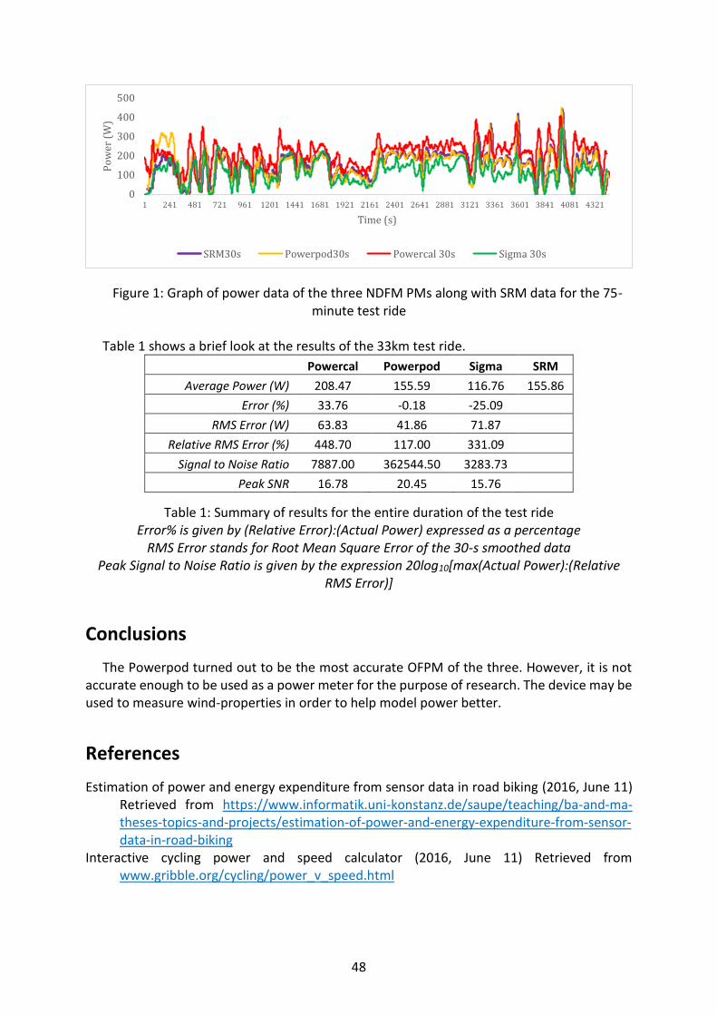
Figure 1: Graph of power data of the three NDFM PMs along with SRM data for the 75-minute test ride

Table 1 shows a brief look at the results of the 33km test ride.

Powercal Powerpod Sigma SRM

Average Power (W) 208.47 155.59 116.76 155.86

Error (%) 33.76 -0.18 -25.09 RMS Error (W) 63.83 41.86 71.87

Relative RMS Error (%) 448.70 117.00 331.09 Signal to Noise Ratio 7887.00 362544.50 3283.73

Peak SNR 16.78 20.45 15.76

Table 1: Summary of results for the entire duration of the test ride Error% is given by (Relative Error):(Actual Power) expressed as a percentage

RMS Error stands for Root Mean Square Error of the 30-s smoothed data Peak Signal to Noise Ratio is given by the expression 20log10[max(Actual Power):(Relative

RMS Error)]

Conclusions

The Powerpod turned out to be the most accurate OFPM of the three. However, it is not accurate enough to be used as a power meter for the purpose of research. The device may be used to measure wind-properties in order to help model power better.

References

Estimation of power and energy expenditure from sensor data in road biking (2016, June 11) Retrieved from https://www.informatik.uni-konstanz.de/saupe/teaching/ba-and-ma-theses-topics-and-projects/estimation-of-power-and-energy-expenditure-from-sensor-data-in-road-biking

Interactive cycling power and speed calculator (2016, June 11) Retrieved from www.gribble.org/cycling/power_v_speed.html

0

100

200

300

400

500

1 241 481 721 961 1201 1441 1681 1921 2161 2401 2641 2881 3121 3361 3601 3841 4081 4321

Po

wer

(W

)

Time (s)

SRM30s Powerpod30s Powercal 30s Sigma 30s

48

Martin, James C., et al. "Validation of a mathematical model for road cycling power." Journal of applied biomechanics 14 (1998): 276-291.

Speed & Power calculator (2016, June 11) Retrieved from www.kreuzotter.de/english/espeed.htm The Powerbike Project (2016, June 26) Retrieved from

https://www.informatik.uni-konstanz.de/saupe/research/powerbike/ Wilson, David Gordon, Jim Papadopoulos, and Frank Rowland Whitt. 2004. "Bicycling science."

3rd ed. Cambridge, Mass.: MIT Press.

49

Modeling Altitude Training Benefits with the Record Power Profile in Professional Cyclists

BELLENOUE Samuel1 2, QUICLET Jean-Baptiste2, MILLET Grégoire1

1ISSUL, University of Lausanne, Switzerland

2AG2R-La Mondiale Pro Cycling Team, La Motte-Servolex, France

Introduction

Assessing fitness changes of athletes is challenging in elite sports (Muller et al. 2000) : tests

require a high level of validity, reliability, accessibility and specificity (Hopkins 2000). Frequent maximal testing sessions are not possible since it would alter the training program and induce additional fatigue. In cycling, different protocols (e.g. cycle ergometer, velodrome, uphill…) have been proposed (Paton and Hopkins 2001) but recently the constant use of validated powermeters during training and racing makes the power output (PO, W) available and permits to model the hyperbolic relationship between the different record PO and time durations; the so-called “Record Power Profile” (RPP) (Pinot and Grappe 2011).

Altitude training is now widely used in endurance sports (Millet et al. 2010) including in

cycling but, to date, there is a scarcity of data on the beneficial or deleterious effects of such intervention in professional cyclists (Garvican et al. 2007; Hahn and Gore 2001). Field evaluation is always difficult, especially during the overloaded competitive period. By using RPP, one may detect fitness changes induced by an altitude training camp. Therefore, the purpose of this study was to assess the performance gains after an altitude training camp in professional cyclists by the mean of the RPP.

Methods

20 professional cyclists (age: 29.1 ± 4.2 years, weight: 66.3 ± 6.8 kg, height: 1.79 ± 0.08 m) performed 15 days of training either by sleeping at an altitude of 2 058 m and training between 490 and 2 642 m (H Hypoxia, n = 7) or by sleeping and training near sea-level (N Normoxia; n = 13). The training content was 17 training sessions, 3.1 ± 1.8 h/session. They performed 12 low intensity training (under the first ventilatory threshold) and 5 high intensity training (above the second ventilatory threshold).

The RPP was modeled from the PO of each rider over four different periods (pre: four weeks prior the intervention period, in: during the altitude camp, post1-2: two weeks after the training camp, post3-4: two weeks after post1-2) in order to assess the change during and

50

after the altitude training at different times since it is known that altitude leads to a decrease in aerobic power (Wehrlin and Hallen 2006) and that the time course of the post-altitude adaptations is not linear (Chapman et al. 2014).

Figure 1: Evolution of the record power profile for the group that lived in altitude

Figure 2: Comparison of the “Record Power Profile” aerobic component for the groups that lived in hypoxia (H) vs. in normoxia (N)

250

300

350

400

450

10 min 20 min 30 min

Po

we

r O

utp

ut

(W)

Time

H

10 min 20 min 30 min

Time

N

Pre

In

Post1-2

Post3-4

250

350

450

550

650

750

850

950

1050

5 sec 30 sec 1 min 5 min 10 min 20 min 30 min

PO

WER

OU

TPU

T

TIME

Pre

In

Post1-2

Post3-4

51

400

500

600

700

800

900

1000

1100

1200

5 sec 30 sec 1 min

Po

we

r O

utp

ut

(W)

Time

H

5 sec 30 sec 1 min

Time

N

Pre

In

Post1-2

Post3-4

Figure 3: Comparison of the “Record Power Profile” anaerobic component for the groups that lived in hypoxia (H) vs. in normoxia (N)

Table 1: Performance change (W and %) of the “Record Power Profile” anaerobic and aerobic components from pre- to post1-2 and post3-4 for the groups that lived

in hypoxia (H) vs. in normoxia (N)

Anaerobic component 5 sec 30 sec 60 sec Mean

Post 1-2

H (W) 58 75 8 47.1

(%) 5.9% 11.1% 1.4% 6.3%

N (W) 35 -13 -57 -12.0

(%) 3.1% -1.9% -9.8% -1.5%

Post 3-4

H (W) 44 7 -10 13.8

(%) 4.5% 1.0% -1.7% 1.8%

N (W) -22 11 11 0.0

(%) -1.9% 1.6% 1.8% 0.0%

Aerobic component 10 min 20 min 30 min Mean

Post 1-2

H (W) 13 1 5 6.0

(%) 3.2% 0.3% 1.4% 1.7%

N (W) -24 -24 -19 -22.2

(%) -6.0% -6.4% -5.6% -6.0%

Post 3-4

H (W) 14 13 15 14.2

(%) 3.6% 3.5% 4.4% 3.8%

N (W) -2 -3 -3 -2.8

(%) -0.4% -0.9% -1.0% -0.8%

52

Conclusions

The mean increase in PO is larger in H than in N for both the anaerobic component at post1-2 (6.3 vs -1.5%) and for the aerobic component at post3-4 (3.8 vs -0.8%). These results are in line with the literature since short-term adaptive non-hematological responses to altitude training likely to improve muscle buffering capacity or glycolytic capacity have been reported (Gore et al. 2007; Mizuno et al. 1990) while the optimal post-altitude period for the aerobic capacity improvement seems delayed to weeks 3 and 4 (Millet et al. 2010; Chapman et al. 2014).

Altogether, this study shows the usefulness of the RPP as a modeling tool for monitoring fitness changes and for assessing the performance gains induced by altitude exposure in professional cyclists.

Bibliography

Chapman RF, Laymon Stickford AS, Lundby C, Levine BD (2014) Timing of return from altitude training for optimal sea level performance. J Appl Physiol (1985) 116 (7):837-843. doi:10.1152/japplphysiol.00663.2013

Garvican LA, Martin DT, Clark SA, Schmidt WF, Gore CJ (2007) Variability of erythropoietin response to sleeping at simulated altitude: a cycling case study. Int J Sports Physiol Perform 2 (3):327-331

Gore CJ, Clark SA, Saunders PU (2007) Nonhematological mechanisms of improved sea-level performance after hypoxic exposure. Med Sci Sports Exerc 39 (9):1600-1609. doi:10.1249/mss.0b013e3180de49d3

Hahn AG, Gore CJ (2001) The effect of altitude on cycling performance: a challenge to traditional concepts. Sports Med 31 (7):533-557

Hopkins WG (2000) Measures of reliability in sports medicine and science. Sports Med 30 (1):1-15

Millet GP, Roels B, Schmitt L, Woorons X, Richalet JP (2010) Combining hypoxic methods for peak performance. Sports Med 40 (1):1-25. doi:10.2165/11317920-000000000-00000

1 [pii]

Mizuno M, Juel C, Bro-Rasmussen T, Mygind E, Schibye B, Rasmussen B, Saltin B (1990) Limb skeletal muscle adaptation in athletes after training at altitude. J Appl Physiol 68 (2):496-502

Muller E, Benko U, Raschner C, Schwameder H (2000) Specific fitness training and testing in competitive sports. Medicine and science in sports and exercise 32 (1):216-220

Paton CD, Hopkins WG (2001) Tests of cycling performance. Sports Med 31 (7):489-496

Pinot J, Grappe F (2011) The record power profile to assess performance in elite cyclists. International journal of sports medicine 32 (11):839-844. doi:10.1055/s-0031-1279773

Wehrlin JP, Hallen J (2006) Linear decrease in .VO2max and performance with increasing altitude in endurance athletes. European Journal of Applied Physiology and Occupational Physiology 96 (4):404-412. doi:10.1007/s00421-005-0081-9

53

Comparison between Maximal Lactate Steady-State, Critical Power and the Second Ventilatory Threshold

detected by a Computer Algorithm

R. Bertschinger1, P. Thumm1, M. Gratkowski2, A. Artiga Gonzalez2, D. Saupe2

1Department of Sport Science, raphael.bertschinger@uni-konstanz.de

2Department of Computer and Information Science, dietmar.saupe@uni-konstanz.de

Introduction

The exact determination of the anaerobic threshold is indispensable in the analysis and optimization of endurance performance, as it demarcates the bodies’ boundary from a predominant aerobic to a predominant anaerobic energy metabolism. In the past, several biological parameters and determination concepts have been proposed to be more or less effective in determining the anaerobic threshold (Peinado, Rojo, Calderon & Maffulli, 2014). Unfortunately most of these concepts are limited by its subjective methodology. In recent years the critical power (CP) concept (Monod & Scherrer, 1965) has received increasing attention and is used alternatively for the anaerobic threshold (Bosquet, Larrouturou, Lheureux & Carter, 2011). However it remains questionable if this concept can be used as an alternative to other lactate threshold concepts. Furthermore it is expected that a more standardised and objective procedure in the determination of the second ventilatory threshold could lead to an improved validity when comparing it to the gold standard method of anaerobic lactate threshold determination. Therefore, the aim of this study was to determine the second ventilatory threshold (VT2) by an automated method as well as CP by three cycle ergometer tests and to compare them to the maximal lactate steady-state (MLSS).

Methods

13 recreational cyclists and one sedentary male (age: 41.1 yrs., height: 181 cm, weight: 75.6 kg, VO2max: 57.2 ml/min/kg) completed a series of cycling tests, separated by at least 48h of recovery. The first test consisted of an incremental ramp exercise to exhaustion for the determination of VT2. The remaining 4-5 tests were performed at different constant work rates (CWR) in order to determine CP and MLSS. Every CWR test lasted up to maximally 30 min or until volitional exhaustion. Lactate probes from the earlobe were taken every five minutes and at test termination. The intensity of each CWR test was related to body weight (range across subjects: 2.75 and 5.5 W/kg) and decreased or increased in steps of 0.25 W/kg. The test phase was completed when all of the following criteria were met:

a) Every subject performed three CWR tests to volitional exhaustion before the end of the 30 minute cut-off time.

b) At least one 30 min test that showed a steady-state (< 1mmol/l) in blood lactate concentration from minute 10-30 and a CWR test at an intensity 0.25 W/kg higher than

54

the previous test that showed an increase in blood lactate concentration of more than 1mmol/l in the last 20 minutes (or less).

The MLSS intensity was defined as the highest intensity in which the lactate concentration did not rise more than 1 mmol/l in the last 20 minutes of the test. The critical power was calculated from the three tests to exhaustion by the 2-parameter critical power model adapted by Moritani, Nagata, deVries und Muro (1981). VT2 was analysed by a self-programmed computer algorithm based on the determination method proposed by Beaver, Wasserman und Whipp (1986).

Results

Mean work rates were 257.9 ± 43.6 W, 279.9 ± 50.1 W and 280.6 ± 42.5 W (Mean ± SD) for MLSS, CP and VT2 respectively. Bland Altman analysis between MLSS and CP revealed a mean bias of 22W with limits of agreement (LoA) between -22 and +66W. For MLSS and VT2 the mean bias was 23W with LoA between -68 and 114W.

A paired t-test showed a significant difference between MLSS and CP (p = .003) but no significant difference for MLSS vs. VT2 (p=.090). Pearson’s Product Moment Correlation revealed a strong correlation between MLSS and CP (r=.893, p=<.001) and a weak correlation between MLSS and VT2 (r=.419, p=.068).

Discussion

The aim of this study was to determine CP with three constant power tests to volitional exhaustion and VT2 by a computer algorithm and compare these procedures to the gold standard method of MLSS determination. Bland Altman analysis represents an adequate tool for demonstrating the amount of agreement between differing methods. In this study the accuracy to identify the MLSS is 18.9 ± 1.4 W. We therefore determined appropriate limits of agreement to lie between ± 20.2W. Bland Altman analyses revealed that an upward bias of 22W (CP) and 23W (VT2) was evident. Unfortunately, the critical limits were more than two-fold for CP (± 44.3W) and four and a half fold for VT2 (± 91W). Therefore, both CP and VT2 determination methods are considered as invalid procedures for the determination of the MLSS. Although testing for statistical differences and relationships showed partly promising results and are to some extent in line with other studies (Dekerle, Baron, Dupont, Vanvelcenaher und Pelayo (2003) Pringle und Jones (2002). However, they are not considered as appropriate procedures

200 250 300 350 400

−40

−2

00

20

40

60

80

Bland Altman Plot: CP vs. MLSS

Means (W)

Dif

fere

nce

s C

P −

ML

SS

(W

)

22.0 W

+1.96 SD

−1.96 SD

66.3 W

Mean

−22.3 W

200 250 300 350 400

−1

00

−5

00

50

10

015

0Bland Altman Plot: VT vs. MLSS

Means (W)

Dif

fere

nc

es V

T −

ML

SS

(W

)

22.7 W

+1.96 SD

−1.96 SD

113.7 W

Mean

−68.3 W

55

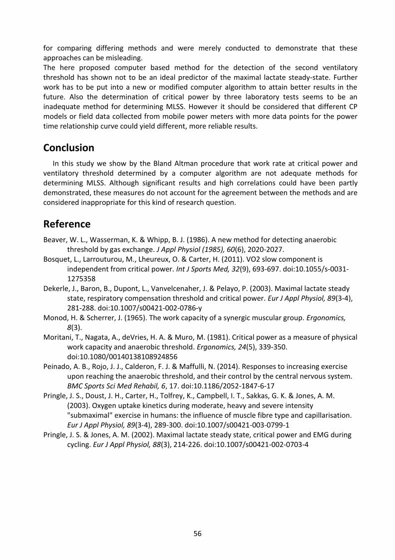
for comparing differing methods and were merely conducted to demonstrate that these approaches can be misleading. The here proposed computer based method for the detection of the second ventilatory threshold has shown not to be an ideal predictor of the maximal lactate steady-state. Further work has to be put into a new or modified computer algorithm to attain better results in the future. Also the determination of critical power by three laboratory tests seems to be an inadequate method for determining MLSS. However it should be considered that different CP models or field data collected from mobile power meters with more data points for the power time relationship curve could yield different, more reliable results.

Conclusion

In this study we show by the Bland Altman procedure that work rate at critical power and ventilatory threshold determined by a computer algorithm are not adequate methods for determining MLSS. Although significant results and high correlations could have been partly demonstrated, these measures do not account for the agreement between the methods and are considered inappropriate for this kind of research question.

Reference

Beaver, W. L., Wasserman, K. & Whipp, B. J. (1986). A new method for detecting anaerobic threshold by gas exchange. J Appl Physiol (1985), 60(6), 2020-2027.

Bosquet, L., Larrouturou, M., Lheureux, O. & Carter, H. (2011). VO2 slow component is independent from critical power. Int J Sports Med, 32(9), 693-697. doi:10.1055/s-0031-1275358

Dekerle, J., Baron, B., Dupont, L., Vanvelcenaher, J. & Pelayo, P. (2003). Maximal lactate steady state, respiratory compensation threshold and critical power. Eur J Appl Physiol, 89(3-4), 281-288. doi:10.1007/s00421-002-0786-y

Monod, H. & Scherrer, J. (1965). The work capacity of a synergic muscular group. Ergonomics, 8(3).

Moritani, T., Nagata, A., deVries, H. A. & Muro, M. (1981). Critical power as a measure of physical work capacity and anaerobic threshold. Ergonomics, 24(5), 339-350. doi:10.1080/00140138108924856

Peinado, A. B., Rojo, J. J., Calderon, F. J. & Maffulli, N. (2014). Responses to increasing exercise upon reaching the anaerobic threshold, and their control by the central nervous system. BMC Sports Sci Med Rehabil, 6, 17. doi:10.1186/2052-1847-6-17

Pringle, J. S., Doust, J. H., Carter, H., Tolfrey, K., Campbell, I. T., Sakkas, G. K. & Jones, A. M. (2003). Oxygen uptake kinetics during moderate, heavy and severe intensity "submaximal" exercise in humans: the influence of muscle fibre type and capillarisation. Eur J Appl Physiol, 89(3-4), 289-300. doi:10.1007/s00421-003-0799-1

Pringle, J. S. & Jones, A. M. (2002). Maximal lactate steady state, critical power and EMG during cycling. Eur J Appl Physiol, 88(3), 214-226. doi:10.1007/s00421-002-0703-4

56

High cycling cadences allow for an increase in training volume monitored via blood lactate concentration

Ralph Beneke, Renate M. Leithäuser

Dept. Medicine, Training and Health, Philipps University Marburg, ralph.beneke@staff.uni-marburg.de

Introduction

Top endurance athletes train 15 to 20 h per week. Selected endurance events seem to require even up to 30 h of training and up to 12 training sessions per week. In order to prevent glycogen depletion 70 to 90 % of the training volume is performed at intensities corresponding to blood lactate concentrations (BLC) up to 2 mmol l-1 [1]. The most efficient cadence in terms of VO2 at low exercise intensities is in the range of 40 to 60 rpm [2]. Cadence related divergences in VO2 converge as exercise intensity increases with small or no differences at peak power (PPeak). The BLC is higher at higher cadences and low intensities and this difference increases furthermore with increasing intensity (3). The reason why competitive cyclists prefer cadences between 90 and 110 RPM is not clear.

The maximal lactate steady state (MLSS) depicts the highest BLC that can be maintained over time without a continual accumulation at constant 30 min workload. Based on the cadence specific MLSS of a female cyclist (age: 25 yrs, height: 1.72 m, body mass: 67 kg, PPeak: 4.9 W kg-1, VO2max: 64.1 ml kg-1 min-1) we simulated cadence dependent limits of sustainable cycling training volume. We tested the hypothesis that high cadences offer an advantage in terms of carbohydrate e.g. pyruvate and lactate oxidation (CHO) related to metabolic rate and sustainable training volume.

Previous work

We demonstrated that at incremental load tests the intensity related to PPeak at which aerobic metabolism approaches complete dependence on carbohydrate oxidation as indicated by a respiratory exchange ratio (RER) near 1.0 was independent of cycling cadence irrespective of a higher BLC at 100 than at 50 RPM [3]. Furthermore, we found a higher MLSS at 105 than at 60 RPM with no differences in MLSS exercise intensity (IMLSS) [1]. At IMLSS RER is almost 1.0 indicating that the mitochondrial metabolism approaches saturation with pyruvate and lactate as metabolic substrate without much variability between the 10th and 30th min [4].

At BLC steady state (BLCSS), the glycolytic pyruvate and lactate generation (Gly) equals CHO (Eq.1). CHO is defined by VO2 times the amount of lactate and pyruvate combusted per unit VO2 (Ox) and the fraction of the VO2 utilized for CHO (relCHO). Gly and Ox depend on

57

VO2max, exercise intensity and cadence [1]. Eq.1: Gly = Ox * relCHO = CHO relCHO can be described as a nonlinear function of BLCSS (Eq.2) [1,3,5-7].

Eq.2:

nSS

CHO

BLC

k1

1relCHO

where kCHO is the constant of the 50 % activation of CHO, functionally reflecting the activation of the pyruvate dehydrogenase of the whole body. With relCHO approaching saturation, the cadence specific kCHO can be estimated by re-arranging Eq.2.

The total power (PTOT) required to cycle at a given velocity is determined by power to overcome air- (PAIR, Eq.3) plus rolling resistances (PROLL, Eq.4) [2,8].

Eq.3: PAIR = 0.5 cd A k v3 where cd is the drag coefficient, A the body surface area, k is the air resistance effective

fraction of A, is air density and v is cycling velocity. Eq.4: PROLL = M g v rrc where M is body mass plus bicycle mass, g is gravity and rrc is the rolling resistance

coefficient. Under the assumption that a daily glycogen turnover of 6 g per kg body mass indicates a

critical margin of sustainable endurance training volume corresponding training limits can be simulated based on cadence specific MLSS and PTOT.

Results

At 105 RPM the MLSS was 0.9 mmol l-1 higher than at 60 RPM (Fig.1) reflecting kCHO values of 6.2 and 3.3 (mmol l-1)3. With 3.3 W kg-1 and 66.7 %, PMLSS105 and IMLSS105 related to PPeak were approximately 8 % lower than PMLSS60 and IMLSS60 of 3.6 W kg-1 and 72.7 %, respectively. However, VO2 and IMLSS related to VO2max were almost identical with 49.3 ml kg-1 and 76.8 % at 105 RPM and 49.0 ml kg-1 and 76.4 % at 60 RPM. This corresponded to cycling velocities of 10.2 and 10.5 m s-1 sustainable for 52.6 and 51.8 min equivalent to 33.7 and 33.2 km at 105 and 60 RPM, respectively.

Cycling at 105 RPM decreased power and v by 18.2 and 7.9 % at 2.0 mmol l-1 and 37.5 and 7.7 % at 1.5 mmol l-1, respectively. No corresponding differences were seen in the VO2. However, compared to 60 RPM cycling at 105 RPM increased the sustainable time of the latter metabolic rate by 23.9 % at 2.0 mmol l-1 and by 40.4 % at 1.5 mmol l-1 (Table 1).

58

Time (min)

0 5 10 15 20 25 30 35

BL

C (

mm

ol l-1

)

0

1

2

3

4

5

6

MLSS

105 RPM , 220 W

MLSS

60 RPM, 240 W

105 RPM, 120 W

60 RPM, 150 W

105 RPM, 70 W

60 RPM, 105 W

Figure 1: MLSS obtained and simulated BLC-response (dotted lines) to prolonged constant workload at training relevant BLC, 105 and 60 RPM

105 RPM 60 RPM

P (W kg-1) 1.8 2.2 IP (% PPeak) 36.4 45.5 VO2 (ml kg-1 min-1) 33.2 33.7 2.0 mmol l-1 IVO2 (% VO2max) 52.6 51.8 v (m s-1) 8.2 8.9 T (min) 133.7 107.9 D (km) 65.8 57.6

P (W kg-1) 1.0 1.6 IP (% PPeak) 21.2 31.8 VO2 (ml kg-1 min-1) 25.9 25.3 1.5 mmol l-1 IVO2 (% VO2max) 40.5 39.5 v (m s-1) 7.2 7.8 T (min) 277.9 198.0 D (km) 120.0 92.7

Table 1: Simulated performance and metabolic response and sustainable training volume corresponding to BLC of 2.0 and 1.5 mmol l-1

59

Conclusions

The present findings provide support for the concept of cycling at relative high cadences at low exercise intensity training. High cadences seem to preserve CHO at given metabolic rates and/or BLC levels during low intensity high volume training sessions allowing for substantially increased training volumes at exercise intensities dominantly utilized in endurance training of high performance athletes.

Reference

[1] Beneke R, Leithäuser RM (2016) Maximal Lactate Steady State depends on Cycling Cadence. Int J Sports Physiol Perform (in press)

[2] Di Prampero PE (2000) Cycling on earth, in space, on the moon. Eur J Appl Physiol 82:345–360

[3] Beneke R, Alkhatib A (2015) High cycling cadence reduces carbohydrate oxidation at given low intensity metabolic rate. Biol Sport 32:27-33

[4] Baron B, Noakes TD, Dekerle J, Moullan F, Robin S, Matran R, Pelayo P (2008) Why does exercise terminate at the maximal lactate steady state intensity? Br J Sports Med 42(10):828-33. Epub 2007 Dec 10. Erratum in: Br J Sports Med. 2009 Apr;43(4):310-1.

[5] Beneke R, Hütler M, Leithäuser RM (2009) Carbohydrate and fat metabolism related to blood lactate in boys and male adolescents. Eur J Appl Physiol 105:257-263

[6] Beneke R (2003) Experiment and computer aided simulation complementary tools to understand exercise metabolism. Biochem Soc Trans 31:1263-1266.

[7] Mader A, Heck H (1986) A theory of the metabolic origin of "anaerobic threshold". Int J Sports Med 7(Suppl 1):45-65.

[8] Beneke R, di Prampero PE (2001) Mechanische und metabolische Belastung beim Radfahren – eine Analyse aus physiologischer und biomechanischer Sicht. Dtsch Z Sportmed 51(1):29-33

60