proceedings of the 27 minisymposium
TRANSCRIPT

PROCEEDINGS OF THE27TH MINISYMPOSIUM
OF THE
DEPARTMENT OF MEASUREMENT AND INFORMATION SYSTEMSBUDAPEST UNIVERSITY OF TECHNOLOGY AND ECONOMICS
(MINISY@DMIS 2020)
FEBRUARY 5–6, 2020BUDAPEST UNIVERSITY OF TECHNOLOGY AND ECONOMICS
BUILDING I
BUDAPEST UNIVERSITY OF TECHNOLOGY AND ECONOMICS
DEPARTMENT OF MEASUREMENT AND INFORMATION SYSTEMS

c© 2020 Department of Measurement and Information Systems,Budapest University of Technology and Economics.
For personal use only – unauthorized copying is prohibited.
Head of the Department:Tamas Daboczi
General Chair:Balazs Renczes
Organizers:Bence BruncsicsKristof Marussy
Peter Nagy
Homepage of the Conference:http://minisy.mit.bme.hu/
Sponsored by:Schnell Laszlo Foundation
E-Group
Supported by the EFOP-3.6.2-16-2017-00013 grant of the European Union,co-financed by the European Social Fund.

FOREWORD
On behalf of the Organizing Committee, I welcome you to the 27th Minisymposium of the Departmentof Measurement and Information Systems at the Budapest University of Technology and Economics.
As it used to be from the beginning of the history of the Minisymposium, the main idea of this event isto provide the Ph.D. students of the department the opportunity to present and discuss their scientificresults. Furthermore, the students can also gain some insights into the practical steps of organizing ascientific event. We are happy to see that in the last few years, the Minisymposium expanded to givespace for our international industrial and scientific partners, as well as to our talented Bachelor andMaster students.
During the years, besides the circle of lecturers, the scope of covered topics has broadened, as well;though our department still have research topics in the field of measurement and instrumentation, theinvestigated areas have been gradually growing to cover embedded information systems, dependabilityand security, artificial intelligence, bioinformatics, and cyber-physical systems.
Similarly to the last years’ practice, and also conforming to the international trends, the proceedingswill only be published in electronic form. We have experienced that the easy accessibility of the digitalproceedings makes it insufficient to publish a printed edition. We hope that any emerging inconveniencewill be dominated by the advantages of the electronic form.
We wish that the forthcoming one and a half days will not only be fruitful in a sense that we will be ableto gain insight into the research of one another, but it will also be a time for discussions and collectingideas for future research, as well as for finding possible interdisciplinary cooperation areas.
Budapest, February, 2020
Balazs RenczesGeneral Chair
2

PAPERS OF THE MINISYMPOSIUM
Author Title Page
Horvath, Kristof andBank, Balazs
Comparison of LMS-based Adaptive Audio Filters 4
Alekszejenko, Levente andDobrowiecki,Tadeusz P.
Simulating Urban Traffic as a Multilayered MultiagentSystem
8
Foldvari, Andras andPataricza, Andras
Support of System Identification by KnowledgeGraph-based Information Fusion
12
Nagy, Peter andJobbagy, Akos
Heart Period Is Defined by P-waves in ECG 17
Staderini, Mirko andPalli, Caterina
An Analysis on Ethereum Vulnerabilities and Further Steps 21
Graics, Bence andMajzik, Istvan
Modeling and Analysis of an Industrial CommunicationProtocol in the Gamma Framework
25
Mondok, Milan andVoros, Andras
Abstraction-based Model Checking of Linear TemporalProperties
29
Elekes, Marton andSzarnyas, Gabor
Incremental View Maintenance in Graph Databases: ACase Study in Neo4j
33
De Brouwer, Edward andArany, Adam andSimm, Jaak andMoreau, Yves
Continuous Time Modelling of Autocatalytic ChemicalReactions Dynamics From Sporadic Inputs
37
3

Comparison of LMS-based Adaptive Audio FiltersKristóf Horváth, Balázs Bank
Budapest University of Technology and EconomicsDepartment of Measurement and Information Systems
Budapest, HungaryEmail: {hkristof, bank}@mit.bme.hu
Abstract—In the field of audio signal processing, logarithmicfrequency resolution IIR filters, such as fixed-pole parallel filtersand Kautz filters, are commonly used. These proven structurescan efficiently approximate the frequency resolution of hearing,which is a highly desired property in audio applications. Inrecursive adaptive filtering however, the FIR structure with LMSalgorithm is the most commonly used. Since the linear frequencyresolution of FIR filters is less than ideal for audio applications, inthis paper we explore the possibility of combining the logarithmicfrequency resolution IIR filters with the LMS algorithm. To thisend the LMS algorithm is applied to fixed-pole parallel and Kautzfilters, and the resulting structures are compared against eachother and to the FIR-LMS filters in terms of convergence timeand remaining error.
Index Terms—audio signal processing, LMS, fixed-pole parallelfilters, Kautz filters
I. INTRODUCTION
Infinite impulse response (IIR) filters are commonly usedin audio signal processing [1], where logarithmic frequencyresolution is highly desired when modeling a transfer function.To achieve this, specialized filter design methodologies havebeen developed, including warped filters [2], second-orderfixed-pole parallel filters [3], and Kautz filters [4].
In adaptive filtering, finite impulse response (FIR) filterstructures with least mean squares (LMS) method are pop-ular choices. The reason for their popularity is their globalconvergence, however, they require more parameters to modela given response, as opposed to IIR filters. Another drawbackis that their residual error (misadjustment) is related to thestep-size coefficient (µ), and thus, a trade-off must be madebetween convergence time and residual error [5].
Common applications for adaptive audio filters, such ascompensation, or noise reduction, contain an adaptive filterthat identifies a given signal path. Thus, as a first step for com-paring logarithmic frequency resolution IIR filters in adaptivecontext, this paper explores the identification capabilities ofthe different IIR structures using LMS algorithm.
In this paper, the LMS algorithm is applied to the paralleland Kautz filters, and the resulting adaptive IIR filters arecompared to each other and to the common FIR-LMS filters.
II. THE LMS ALGORITHM
The Least Mean Squares (LMS) algorithm is a stochasticgrade descent method where the coefficients are adapted basedon the current error in time [5]. It uses the estimate of themean square error (MSE) gradient vector from the available
Fig. 1. LMS-based adaptive filter used for identification.
data, to make successive corrections to the filter coefficientsin the direction of the negative of the gradient vector. Thisiterative procedure eventually leads to minimum mean squareerror.
The block scheme of the LMS filter can be found in Fig. 1.The common input of the system to be identified and theadaptive filter is denoted by u(k), and the outputs are markedby y(k) and y(k) respectively.
The output of the adaptive filter is computed as
y(k) = w>(k)x(k). (1)
The recursive function for coefficient adaptation is thefollowing:
w(k + 1) = w(k)− µe(k)x(k), (2)
where w denotes the filter coefficients, k is the discrete time,µ is the step-size parameter, x is the estimated gradient and eis the output error, where e(k) = y(k)− y(k).
The input vector x(k), which acts as the estimated gradientvector, is unique for every filter structure. For FIR filters, itis a delay line; for other structures it can be deduced usingEquation 1.
Note that each element of x(k) is a function of time, andthey span the space of the output function. Because theyact as base functions, their correlation has an impact on theconvergence time: the lower the eigenvalue spread of thecorrelation matrix R, the faster the convergence [5].
4

The estimated autocorrelation matrix of x(k) is calculatedas:
R =1
L
L∑
k=0
x(k) · x>(k), (3)
where L denotes the number of samples.The main drawback of the LMS algorithm is that the gra-
dient vector scales with the input, which can cause instabilityin the adaption. As a remedy, the Normalized-LMS (NLMS)method is used, which normalizes the power of the input [5]:
w(k + 1) = w(k)− µ e(k)x(k)
α+ x>(k)x(k), (4)
where α is a small positive number used to avoid the denom-inator to become zero.
In this paper we used the NLMS algorithm for realizingadaptive filters.
III. ADAPTIVE IIR FILTERS
Adaptive IIR filters require fewer parameters compared toFIR filters, however, early research showed that adaptivelyvarying both the poles and zeros can lead to suboptimal per-formance caused by multimodal error surfaces [6] or becausethey require satisfaction of a strict positive real condition [7].
Alternatively, the poles of the IIR filter can be fixed at pre-determined values, which preserves the linearity in parametersand leads to well-behaved adaptation properties [8].
In audio signal processing, fixed-pole filters are commonlyused. The Kautz (Fig. 3) and the fixed-pole parallel filters(Fig. 2) are proven to have equivalent transfer functions whendesigned off-line [3]. The main difference between them lies inthe computational demand (see Table I): the fixed-pole parallelfilter need approximately 47% less operations compared tothe Kautz filter. The tap outputs of the two filters span thesame space, but the base functions of the Kautz filter areorthonormal [9]. This results in convergence properties similarto that of FIR filters [8].
The general structure of the parallel second-order structurecan be found in Fig. 2. The second-order sections can beimplemented as either direct-form, or other structures [10].Note that the structure of the second-order sections have directimpact on the parameters, and thus, affects the convergenceproperties if the second-order section is used in an adaptivefilter realization.
Adapting the aforementioned fixed-pole audio filters usingthe LMS algorithm can be done by substituting the IIR filterto the ∇ block in Fig. 1, with the output multiplications andsummation replaced by the adaptive linear combination of theLMS algorithm. For example, in case of the Kautz filter inFig. 3 it means that the ci coefficients are the tuned parameters.
IV. ORTHOGONAL SECOND-ORDER SECTION
In order to improve convergence, we present a new second-order structure (Fig. 4), which, to our knowledge, has notbeen presented before. The new structure is equivalent to asecond-order Kautz filter, therefore its two tap outputs are
TABLE INUMBER OF ARITHMETIC OPERATIONS REQUIED FOR THE TESTED
ADAPTIVE IIR FILTERS HAVING N CONJUGATE-COMPLEX POLE PAIRSIMPLEMENTED USING DIRECT-FORM 2 (DF2) OR ORTHOGONAL
SECOND-ORDER SECTIONS.
Multiplication AdditionFixed-pole parallel filter (DF2) 6N 3N − 1Fixed-pole parallel filter (orth.) 6N 5N − 1
Kautz filter (DF2) 9N + 2 8N + 1
Fig. 2. Parallel second-order filter. Note that in our investigations we omittedthe constant K section.
orthogonal. As this structure is more complex than the direct-form implementation, its usage in parallel filters result incomputational demand between the direct-form parallel filterand the Kautz filter.
The parameters a1 and a2 are the same as in the direct form.The p and q coefficients can be computed from the direct-formparameters b0 and b1 with the following formulas:
p =b0 − b1
2, (5)
q =b0 + b1
2. (6)
The estimates of the autocorrelation matrices can be foundin Fig. 5. It can be seen that the orthonormal property of theKautz filter results in a unity autocorrelation matrix. In fixed-pole parallel filters however, the neighboring tap outputs havehigh levels of cross-correlation. This effect is lower when theorthogonal second-order sections are used: only the tap outputsof the different sections are correlated, resulting in a periodicpattern.
V. NORMALIZING THE TAP OUTPUTS
The convergence rate of the LMS algorithm is relatedto the eigenvalues of the R matrix [5]. It is shown thatif the eigenvalue spread of the R matrix is the minimumover all possible matrices, the maximum convergence ratecan be achieved. As a consequence, the tap outputs of thefilter (denoted by X(k)) having the same output power is anecessary condition. This criterion is inherently satisfied fororthonormal filters [8], but not for fixed-pole second-order
5

Fig. 3. Kautz filter structure.
filters. Therefore, the tap outputs of the second-order sectionsneed to be scaled.
To determine the normalizing coefficients, we compute theimpulse responses between the input and the tap outputs. Thescaling factors are then determined by the sum of squares ofthe impulse responses:
si =1
∞∑k=0
(hi(k)
)2 , (7)
where hi denotes the impulse response between the filter inputand the i-th filter tap output. Using this scaling, the tap outputswill have the same power when the input is white noise.
VI. COMPARISONS
In our investigation we used the NLMS algorithm as amethod for system identification (Fig. 1). The input wasa white noise uniformly distributed in range [−1;+1]. Thesystem to be identified was implemented using a 10000-tap long FIR filter, whose coefficients were based on actualimpulse response measurements.
Fig. 4. Orthogonal second-order structure, with normalizing terms s1 and s2.
10 20 30 40
10
20
30
4010 20 30 40
10
20
30
40
10 20 30 40
10
20
30
40
0.2
0.4
0.6
0.8
1
Fig. 5. Visualization of R matrices. Top left: parallel filter with direct-form sections; top right: parallel filter with orthogonal second-order sections;bottom left: Kautz filter.
The filters to be compared are fixed-pole second-orderparallel filters (without FIR section), implemented using bothdirect-form and improved second-order sections, a Kautz filterand as a reference, a FIR filter. The IIR filters have 20conjugate complex pole pairs, placed along a logarithmic scalebetween 20 Hz and 20 kHz, assuming 44.1 kHz samplingfrequency. The quality factors of the poles were chosen thatthe neighboring sections had their magnitude response crossat their -3 dB point [11]. The FIR filter has 40 taps, thus thefilters have the same amount of free parameters.
The mean square error (MSE) of adapted filter parametersare computed on a logarithmic scale: the error, denoted by e(k)in Fig. 1, has its DFT spectrum sampled at certain frequencieshaving logarithmic distribution. The samples are then squaredand summed from 20 Hz to 20 kHz, assuming fs = 44.1 kHzsampling rate:
E(jω) = DFT{e(k)}, (8)
MSE =
f=20kHz∑
f=20Hz
∣∣E(j2πf/fs)∣∣2. (9)
For comparison, the MSE was calculated for all structures atevery 256 samples and then plotted.
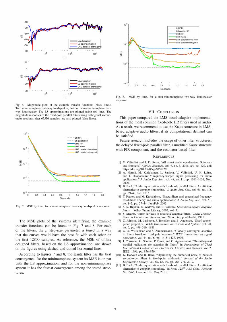
In our investigation, we used two example transfer functionsfor testing the algorithms: a minimumphase one-way loud-speaker (Fig. 6 top) and a larger, two-way loudspeaker withnon-minimumphase response (Fig. 6 bottom). In the figures,we marked the result of the off-line LS design as well as themagnitude response of the adaptive fixed-pole parallel filterthat is implemented using orthogonal second-order sections.Note that the transfer function of the adaptive Kautz is omittedbecause it fits the LS solution after the simulation time (65536samples).
6
Hz102 103 104
dB
-60
-50
-40
-30
-20
-10
LoudspeakerLS approximationLMS parallel orthogonal
Hz102 103 104
dB
-30
-20
-10
0
10
LoudspeakerLS approximationLMS parallel orthogonal
Fig. 6. Magnitude plots of the example transfer functions (black lines).Top: minimumphase one-way loudspeaker; bottom: non-minimumphase two-way loudspeaker. The LS approximations are plotted using red lines. Themagnitude responses of the fixed-pole parallel filters using orthogonal second-order sections, after 65536 samples, are also plotted (blue lines).
Seconds0 0.2 0.4 0.6 0.8 1 1.2 1.4 1.6 1.8
MS
E
10-4
10-3
10-2
10-1
100
LSiFIRLSiparalleliIIRLMSiFIRLMSiKautzLMSiparallelidirect-formLMSiparalleliorthogonal
Fig. 7. MSE by time, for a minimumphase one-way loudspeaker response.
The MSE plots of the systems identifying the exampletransfer functions can be found in Fig. 7 and 8. For eachof the filters, the µ step-size parameter is tuned in a waythat the curves would have the best fit with each other onthe first 12800 samples. As reference, the MSE of offlinedesigned filters, based on the LS approximation, are shownon the figures using dashed and dotted horizontal lines.
According to figures 7 and 8, the Kautz filter has the bestconvergence: for the minimumphase system its MSE is on parwith the LS approximation, and for the non-minimumphasesystem it has the fastest convergence among the tested struc-tures.
Seconds0 0.2 0.4 0.6 0.8 1 1.2 1.4 1.6 1.8
MS
E
10-3
10-2
10-1
100
LSiFIRLSiparalleliIIRLMSiFIRLMSiKautzLMSiparallelidirect-formLMSiparalleliorthogonal
Fig. 8. MSE by time, for a non-minimumphase two-way loudspeakerresponse.
VII. CONCLUSION
This paper compared the LMS-based adaptive implementa-tions of the most common fixed-pole IIR filters used in audio.As a result, we recommend to use the Kautz structure in LMS-based adaptive audio filters, if its computational demand canbe satisfied.
Future research includes the usage of other filter structures:the delayed fixed-pole parallel filter, a modified Kautz structurewith FIR component, and the resonator-based filter.
REFERENCES
[1] V. Välimäki and J. D. Reiss, “All about audio equalization: Solutionsand frontiers,” Applied Sciences, vol. 6, no. 5, 2016, art. no. 129, doi:https://doi.org/10.3390/app6050129.
[2] A. Härmä, M. Karjalainen, L. Savioja, V. Välimäki, U. K. Laine,and J. Huopaniemi, “Frequency-warped signal processing for audioapplications,” J. Audio Eng. Soc., vol. 48, no. 11, pp. 1011–1031, Nov.2000.
[3] B. Bank, “Audio equalization with fixed-pole parallel filters: An efficientalternative to complex smoothing,” J. Audio Eng. Soc., vol. 61, no. 1/2,pp. 39–49, Jan. 2013.
[4] T. Paatero and M. Karjalainen, “Kautz filters and generalized frequencyresolution: Theory and audio applications,” J. Audio Eng. Soc., vol. 51,no. 1–2, pp. 27–44, Jan./Feb. 2003.
[5] S. S. Haykin, B. Widrow, and B. Widrow, Least-mean-square adaptivefilters. Wiley Online Library, 2003, vol. 31.
[6] S. Stearns, “Error surfaces of recursive adaptive filters,” IEEE Transac-tions on Circuits and Systems, vol. 28, no. 6, pp. 603–606, 1981.
[7] C. Johnson, M. Larimore, J. Treichler, and B. Anderson, “Sharf conver-gence properties,” IEEE Transactions on Circuits and Systems, vol. 28,no. 6, pp. 499–510, 1981.
[8] G. A. Williamson and S. Zimmermann, “Globally convergent adaptiveiir filters based on fixed pole locations,” IEEE transactions on signalprocessing, vol. 44, no. 6, pp. 1418–1427, 1996.
[9] J. Cousseau, G. Sentoni, P. Diniz, and O. Agamennoni, “On orthogonalparallel realization for adaptive iir filters,” in Proceedings of ThirdInternational Conference on Electronics, Circuits, and Systems, vol. 2.IEEE, 1996, pp. 856–859.
[10] K. Horváth and B. Bank, “Optimizing the numerical noise of parallelsecond-order filters in fixed-point arithmetic,” Journal of the AudioEngineering Society, vol. 67, no. 10, pp. 763–771, 2019.
[11] B. Bank, “Audio equalization with fixed-pole parallel filters: An efficientalternative to complex smoothing,” in Proc. 128th AES Conv., PreprintNo. 7965, London, UK, May 2010.
7

Simulating Urban Traffic as a MultilayeredMultiagent System
Levente AlekszejenkoDepartment of Measurement and Information Systems
Budapest University of Technology and Economics Budapest, Hungary
Tadeusz DobrowieckiDepartment of Measurement and Information Systems
Budapest University of Technology and Economics Budapest, Hungary
Abstract—The vehicles of the future will be capable of com-municating with each other and with the road infrastructureas well. Based on this ability, complex multiagent systems canbe designed, including smart cars and intelligent traffic controlsystems (referred to as judges).
Such system was implemented by extending an open-sourcetraffic simulation tool, called Simulation of Urban MObilityplatform (SUMO). The implemented system can be used toexperiment with and to verify various algorithmic approachesaimed to increase the intelligence of autonomous drivers andurban traffic controllers.
Our study investigated the adaptation of the operating systemtask schedulers and the Explicit Congestion Notification algo-rithm of computer networks. It resulted in a layered cooperativemulti agent system composed from platooning car drivers in thelower layer and the cooperating intersection judges in the upperlayer.
Results indicate that the implemented system can organizethe traffic better in extraordinary cases (e.g. an accident, roadworks on some major streets, etc.). The regulatory capability ofthe proposed system depends greatly on the topology of the roadconnections. This aspect (especially the problem of congestions)is currently under investigation.
Index Terms—intelligent traffic control, smart vehicles, multia-gent system, platooning, explicit congestion notification, schedul-ing algorithms
I. INTRODUCTION
One of the major problems of our cities is the regularcongestion of road networks. As the number of vehiclesis rapidly increasing, improving the flow of the traffic andreducing traveling time becomes an even more challengingtask. The connected vehicles of the future and the wide varietyof IoT devices implemented in the road infrastructure maycreate new ways to optimize the traffic.
For example, smart cars can form groups, so called platoons,near intersections. The cars which form a platoon can changelanes or can pass through intersections together, thereforecausing less impact on the traffic.
Another possibility is to create intelligent traffic controllers,so called judges. Let us suppose that the number of incomingvehicles from each direction is known. In this case, as the
The research has been supported by the European Union, co-financed by theEuropean Social Fund (EFOP-3.6.2-16-2017-00013, Thematic FundamentalResearch Collaborations Grounding Innovation in Informatics and Infocom-munications).
demand is known for the near future, theoretically well estab-lished scheduling algorithms can be applied. Moreover, thesejudges can be made cooperative as well in order to make aglobally optimal solution.
Some ideas have already been implemented as a multilay-ered multi-agent system. In our implemented system there aretwo types of agents, i.e. smart cars and judges. They cancommunicate with each other in order to perform some intel-ligent actions. For example, smart cars can form platoons, orask the judges whether they can pass through an intersection.Judges can also send messages to each other, cooperativelyevaluating the state of the roadnetwork, to attempt to avoidthe congestion. The performance of our system was validatedby simulations. The used simulation platform was createdby extending the Simulation of Urban MObility (SUMO) [5]microscopic traffic simulation program.
II. LITERATURE REVIEW
Creating platoons of smart cars, besides reducing the com-putational demands on intelligent traffic controllers, results ina more efficient lane-changing strategy. Let us suppose thatthe lane-changing of a platoon can be modeled as a singlelane-change of a truck. In [9] the authors have shown thata double semi-trailer truck is equivalent to 3 personal cars.It takes, however, more space on the road than those 3 cars.Consequently, platooning also seem to be an effective way toreduce the impact of lane-changes.
Consider now the perspective of a judge, i.e. an intersectioncontroller. The task of the judge is analogous to that of thescheduler of an operating system. Both are responsible fordeciding which competing entity (task or vehicle) can use aunique resource (the processor or the part of the intersection).A scheduling solution to control intersection lamps was sug-gested by [1], where so called Minimal Destination DistanceFirst (MDDF) method was used, based on the well knownShortest Job First scheduler (SJF)1 of operating systems.Unfortunately, that proposed algorithm is not fair and wasverified only in a highly regular intersection environment.
Coordination of the traffic signals is an old idea, and forexample can be achieved by green-waves. There are some
1To be precise it is based on the Shortest Remaining Time First, thepreemptive version of SJF.
8

traditional algorithms, like TRANSYT and SCOOT [7], whichtry to shorten the queue lengths behind the traffic lights. In thelast decades, new methods were published, for example the onebased on a reservation system [2]. In this algorithm, smart carshave to book time and space slots when they are permitted topass through the intersection. An intersection manager storesthese bookings and checks whether an incoming booking isfeasible. This system has a major disadvantage, namely whenthere is a vast amount of vehicles with a vast amount ofbookings, the feasibility check would be a really processing-intensive task. An agent based solution was proposed in [10].In this approach every neighboring intersection was connected,therefore it is theoretically possible to create unstable states.The green time of a traffic signal is only modified a little bit,making its neighbors also to modify a little bit more, and soon. As a result of this butterfly-effect, the whole system mightbecome unstable, causing unpredictable traffic flows, thereforeincreasing the risk of an accident.
III. INTERACTION BETWEEN SMART CARS – PLATOONING
A. Formation of a Platoon
Smart cars are basically competing agents (for the greenlight slot), but they are willing to form a coalition – a platoon –in order to go through an intersection as efficiently as possible,if their interests (path) coincide.
When a smart car approaches an intersection2, it has to joina platoon. The cars of a platoon have the exactly same trajec-tory: they arrive at the intersection from the same direction, inthe same lane and leave via the same exit lane. For the timethe platoon exists, its cars are joined virtually into a chainmaintaining about 5 m of distance between each other.3
If the platoon in front of a smart car is not suitable, thesmart car has to create a new platoon.
In the front of the platoon is the platoon leader, all theother vehicles in the platoon are the platoon members. Platoonleaders are responsible for their platoons, and the platoonmembers have to follow the platoon leader.
After crossing the junction, the platoon leader exits itsplatoon and passes over its prerogatives to the next-in-linein the platoon. This smart car will be the new platoon leader.It is an easy and effective way to avoid the problems whichcan be caused by the preemptive scheduler of the judges.
B. Lane-Changing of Platoons
Reducing the impact of changing lanes before intersectionscan provide a significant improvement in the traffic flow. In theSUMO platform sophisticated lane change models are alreadyimplemented. In our research we modified the SL2015 model[3] to calculate also with the platooning concept. So while asmart car belongs to a platoon, it has to behave differently,depending on whether it is the leader or a simple member.
2Some markers are placed as new traffic signs which instruct the smart carsto join or leave a platoon.
3Platooning in this case is an adhoc formation and slightly differs fromplatoons created on highways. The aim of our platoons is to pass throughintersections more effectively than individual vehicles are able to do so.
In a platoon only the platoon leader can make a lane-changedecision. All the other members have to follow the car in frontof them.
If the platoon leader finds out that a lane change is needed4,it makes contact with the platoon leader (if there is any) in thetarget lane. The two platoon leaders make an agreement whoseplatoon will be ahead of the other.5 Platoon in the target lanewill slow down or even stop if necessary to make sure thatthe maneuver will be successful. Another possibility is that themover leader has to wait until the asked leader and its platoonleaves the target lane. The platoon manages the lane changecar-by-car, sending lane-change command down the platoonchain.
IV. INTERSECTION CONTROLLING ALGORITHMS OFUNCONNECTED JUDGES
In our first approach, unconnected (i.e. non-communicating)judges were implemented. From the operating system field weborrow two simple scheduling algorithms. One is the RoundRobin (RR) algorithm, which is fair (free of starvation) and theother is the Shortest Job First (SJF), which yields an optimalresponse time, but is unfair. These two simple schedulers (andtheir preemptive versions respectively) provide the basics ofall kinds of much more complex scheduling algorithms. Due tothis fact, we decided to try out these two methods, as conflictclass6 selector algorithms of an intelligent judge agent.
1) RR: A simple round robin scheduler can be implementedas a traffic controlling method without any significant modi-fication to the original algorithm. We prescribe time slices toeach conflict class. This will be the maximal amount of timein which a conflict class can be active. After this time slice iselapsed, we simply select the next conflict class from the list.
2) MDDF: [1] Minimal Destination Distance First trafficcontrolling system is based on the optimal scheduler, calledShortest Job First (specifically its preemptive version, the so-called Shortest Remaining Time first). The problem with thissolution is that it is not fair.
Let us suppose that a lonely car is waiting in an intersec-tion to pass. This car is at the beginning of its route to avery distant destination, but vehicles with significantly shorterroutes are continuously arriving. The car with the long routeto its destination can wait forever without getting through thisintersection.
To make the algorithm fair, we redefined our scheduler asa two-level scheduler. On the higher priority level a simpleRound Robin scheduler is running, and on the lower prioritylevel a scheduling algorithm similar to the implementation of[1] is used. At first, every conflict class is scheduled by thelower priority level. If a conflict class was not active in thelast 90 s, it would change its priority to the high level. This
4In this state, smart cars’ lane change model calculates with length ofplatoons instead of single vehicles.
5 [3] has already worked out the protocol and algorithm of this agreement.We modified the existing solution to have the contract made only betweenplatoon leaders instead of single vehicles.
6A conflict class is a group of cars, which are permitted to pass throughan intersection simultaneously.
9

way it is guaranteed that every vehicle will be scheduled in alimited amount of time. The Round Robin also prevents theoccurrence of starvation.
V. INTERSECTION CONTROLLING ALGORITHMS OFCONNECTED JUDGES
A. The ECN-based method
It is a simple idea to connect the judges (i.e. to permitthem to communicate) with each other in order to improve thecapabilities of the system. This improvement is a signal coor-dination which aims to prevent the formation of congestions.Such algorithms are already in use in the domain of computernetworking. However, the character of the traffic is differentand the majority of them cannot be applied in the road trafficenvironment. An algorithm which could be applied, or at leastbe experimented with, is the so called Explicit CongestionNotification (ECN) method [4], which we implemented in oursimulations.
The basic idea behind ECN is that the receiver node (anintersection manager or a network router) can inform thesender if the queue length (of vehicles or datagrams) at thereceiver side reaches a certain level (let us call this signal theECN-signal). This means that a congestion is about to form.To avoid the congestion, the sender must decrease its outputin this case. A new kind of judge, the so-called ECN-judge,was implemented which is based on this discussed method.
The ECN algorithm has a great advantage that it doesnot require the definition of arterial directions7. Definingarterials would demolish the merits of the intelligent system inextraordinary situations, when the proposed system can clearlyoutperform the traditional system, for details, see Section VI.
B. Challenges in the Implementation
The state-space of the ECN judge can be enormous since itdepends both on the number of incoming vehicles and on thenumber of the neighboring intersections. Therefore, storing asignal plan for all of the states is quite memory-consuming.Instead of doing this, a dynamical signal plan generationmethod was implemented (for an overview, see Figure 1).
The calculation of simple signal phase can be formalized asan integer programming problem (IP). Our goal is to maximizethe number of directions which receive green light at the sametime, subject to the actual state of the network. This stateconsists of dynamic parts, like the incoming ECN-signals orthe decision of a scheduling algorithm (eg. a Round Robin) aswell as static parts, which describes which directions cannotpass through an intersection simultaneously.
If the IP is solved, we only know the signal phase fora given moment. In order to generate a signal plan (whichdescribes how long a direction should get a green or a redlight), it is necessary to recalculate this IP problem from timeto time. In our implementation the recalculation time is alinear function of the number of incoming vehicles, but cannotexceed 45 seconds.
7Arterial direction is the main route which for example receives a green-wave.
Fig. 1. Overview of the ECN-judge
There is another topic which should be discussed, namelythe identification of the forming congestions. It is a quitedifficult task [6], [8], and our research did not focus onsolving this problem, thus based on preliminary simulations,we simply calculated the traffic density, which can provide thehighest traffic flow. We say that there is a congestion formingwhen the 90% of this level is reached, so the ECN-signal issent at this event.
VI. SIMULATIONS
Our solutions were tested by an extension to the Simulationof Urban MObility program (see Figure 2 for details). Thesimulated network was the BAH intersection8 of Budapest andits close neighborhood.
Fig. 2. The developed extension of the SUMO. The components of themultilayered, multiagent system are shown in green. Some modules arenecessary to create an abstraction layer between the original source code of theSUMO and the intelligent system’s layer. This abstraction layer is presentedin orange and blue in this figure.
Basically two types of traffic demand were modeled: somecases of regular traffic (eg. night traffic, morning traffic, nountraffic) and irregular traffic (Budaorsi ut is closed9) were fedinto the simulator.
8Where streets of Hegyalja ut, Jagello ut, Villanyi ut, Budaorsi ut andAlkotas utca intersect.
9Irregular1 case: Obstacle is northbound of “Budaorsi ut”, can be bypassedvia Karolina and Villanyi streets.Irregular2 case: Obstacle is southbound of “Budaorsi ut”, bypass route is via“Hegyalja ut”.
10

A. Simulating The Unconnected Judges
As a first attempt, we tested the behavior of the platooningsystem and the simple, unconnected judges. These measure-ments basically show that such kind of systems may be ableto reduce waiting and traveling times through this intersection.
The results show (see Table I and Table II) that such asystem is able to decrease the waiting (for example at redlights) and average traveling times in irregular situations. Onthe other hand, the improvement of the traffic flow10 is not soobvious in regular cases, see Figure 3.
TABLE ISIMULATION RESULTS OF “IRREGULAR1” CASE
Test case Arrived Waiting Time Average Traveling Time(%) (s) (s)
Traditional 33.81 29.68 170.55RR 29.19 12.117 174.87MDDF 22.77 12.41 154.02
TABLE IISIMULATION RESULTS OF “IRREGULAR2” CASE
Test case Arrived Waiting Time Average Traveling Time(%) (s) (s)
Traditional 38.48 36.44 199.38RR 32.71 11.43 170.07MDDF 34.39 10.74 176.72
B. Simulating The Connected Judges
In order to improve the traffic flow, some judges11 were re-programmed to ECN-judges. Theoretically this system wouldhave greater chance to find a globally optimal solution, thanthe unconnected judges, which are only capable of finding alocally optimal scheduling.
The trial of the system gave surprising results. Instead ofimproving the flow of the traffic in the BAH-intersection,this method rather reduced this value. As it can be seen inFigure 3, the new judges limit the density of the traffic toaround 65-70 vehicles/km, almost regardless of the height ofthe traffic demand. (With a combined system, which containsboth connected ECN-type and unconnected Round Robin-typejudges, this limit is slightly higher.) Partly by this densitylimitation, partly by some yet unknown effects, the traffic flowis strongly reduced by the ECN-judge system.
VII. CONCLUSION AND FURTHER RESEARCH AIMS
As the traditional system is likely to be numerically opti-mized, it is a challenging task to achieve the same or evenbetter results with a new intelligent solution in regular cases.On the other hand, in extraordinary situations, an intelligent,
10The traffic flow is a commonly calculated value. It is the product of thetraffic density ( vehicles
km) and the mean velocity of the vehicles ( km
h). These
values can be measured by different types of detectors, cameras, etc.11Namely the judge supervising the intersection of Villanyi and Budaorsi
streets, the one supervising the Budaorsi, Hegyalja and Alkotas street inter-section and the one placed at the Jagello and Hegyalja crossing.
Fig. 3. Traffic flow in the traditional and in the unconnected intelligent system,consisting of RR-type judegs.
multi-agent based solution can be much more flexible. Thisflexibility provides better traveling times by reducing theunnecessary waiting times.
The ECN-judges have no benefits in the BAH intersectionscenario, if our goal is to improve the flow of the traffic.Supposing that there are situations where the traffic density(and therefore the flow) limitation is a desired effect, ourproposed system might be beneficial as well. Such situationscan be the limitation of the traffic going through residentialareas or nature reserves.
Further research is needed to verify that the ECN-judgesystem is able to cause such effect in these kinds of networks.
REFERENCES
[1] F. Ahmad, S. A. Mahmud, G. M. Khan, and F. Z. Yousaf, “Shortestremaining processing time based schedulers for reduction of trafficcongestion,” in 2013 International Conference on Connected Vehiclesand Expo (ICCVE), Las Vegas, NV, USA, 2013, pp. 271–276.
[2] K. Dresner and P. Stone, “A Multiagent Approach to AutonomousIntersection Management,” JAIR, vol. 31, pp. 591–656, Mar. 2008.
[3] J. Erdmann, “SUMO’s Lane-Changing Model”, in Modeling Mobilitywith Open Data, M. Behrisch and M. Weber, Edit. Cham: SpringerInternational Publishing, 2015, pp. 105–123.
[4] S. Floyd, K. K. Ramakrishnan, and D. L. Black, “The Addition ofExplicit Congestion Notification (ECN) to IP.” [Online]. Accessible:https://tools.ietf.org/html/rfc3168#section-1. [Accessed: 2019. okt. 25.].
[5] P. A. Lopez et al., “Microscopic Traffic Simulation using SUMO,”in 2018 21st International Conference on Intelligent TransportationSystems (ITSC), 2018, pp. 2575–2582.
[6] K. Nagel, P. Wagner, and R. Woesler, “Still Flowing: Approaches toTraffic Flow and Traffic Jam Modeling,” Operations Research, vol. 51,no. 5, pp. 681–710, Oct. 2003.
[7] D. I. Robertson, “Research on the TRANSYT and SCOOT Methods ofSignal Coordination,” ITE Journal, Jan 1986 pp. 37-40.
[8] M. Treiber and A. Kesting, Traffic Flow Dynamics. Berlin, Heidelberg:Springer Berlin Heidelberg, 2013.
[9] N. Webster and L. Elefteriadou, “A simulation study of truck passen-ger car equivalents (PCE) on basic freeway sections,” TransportationResearch Part B: Methodological, vol. 33, no. 5, pp. 323–336, 1999.
[10] J. Withanawasam and A. Karunananda, “Multi-agent based road trafficcontrol optimization,” in 2017 IEEE 20th International Conferenceon Intelligent Transportation Systems (ITSC), Yokohama, 2017, pp.977–981.
11

Support of System Identificationby Knowledge Graph-Based Information Fusion
Andras FoldvariDepartment of Measurement and Information Systems
Budapest University of Technology and EconomicsHungary
Andras PatariczaDepartment of Measurement and Information Systems
Budapest University of Technology and EconomicsHungary
Abstract—The paper presents a knowledge graph-based so-lution for creating the core models for supervisory control ofcomplex Cyber-Physical Systems (CPS) and computing infras-tructures from design models and operational logs.
The core element of modern supervisory control approachesis a digital twin, which maps the observations about the systeminto a hybrid run-time model representing the expected systemstate. It serves as a basis for interaction between the controllerand the controlled system.
The high-level discrete-state machine of digital twins rep-resents the different operational regimes (domains of similarbehavior) and transitions between them. A continuous modeldescribes the intra-domain behavior in detail. A special case isthe qualitative domain model using discretized state variablesin the form of a few ordered values (e.g. low, medium, high).This model category is extremely beneficial, when representingpartial, dimensioning dependent behavior.
Parts of the digital twin model can be directly derived fromthe design models, but the description of dynamics of thequalitative domain models necessitates system identification fromobservations (operation logs or benchmark results). This waythe creation of the digital twin necessitates information fusionfrom different sources. Knowledge graphs provide an abstractsemantic framework for this purpose.
Our goal is to support system identification by deductivereasoning performing step-by-step checks of the abstract modelto assure consistency and completeness of the observations andtheir respective evolving models.
Index Terms—cyber-physical systems, system identification,knowledge graph, digital twin
I. INTRODUCTION
The purpose of cyber-physical systems (CPS) [1] is toobserve and control the physical world through intelligentmechanisms. They operate over continuous and discrete sig-nals originating in the physical world, for which they consistof physical and computational components interacting throughcommunication layers [2].
The core concept in modern supervisory control of CPSsis the “digital twin.” Data delivered by sensors continuously
The results presented in this research report were established in theframework of the professional community of Balatonfured Student ResearchGroup of BME-VIK to promote the economic development of the region.During the development of the achievements, we took into consideration thegoals set by the Balatonfured System Science Innovation Cluster and the plansof the ”BME Balatonfured Knowledge Center”, supported by EFOP 4.2.1-16-2017-00021.).
synchronize this model of the system under control with thephysical world. Assurance of dependability and resilience ofcritical CPSs necessitates the faithfulness of the twin model.
Modern CPS design relies on the integration of pre-implemented components. The compliance to the designatedtemporal properties (timeliness, throughput, etc.) necessitatesa proper dimensioning of the resources allocated to the com-ponents prior to the deployment.
The performance domain can influence the logic behavior.Non-linear effects resulting in bottlenecks, like the saturationof a particular resource, may change the dynamic behaviorof the system. Moreover, CPS activates the built-in overloadprotection mechanisms, this way the behavior of a particularcomponent, subsystem, and the entire system depend both onthe functional logic (functional architecture of the system) andon its parametrization.
This way, scalability of the digital twin, similar to thedeployed system requires hybrid modeling (Fig. 1) approachseparating the dimensioning-independent overall logic of thebehavior (discrete domain) and its actual state within an oper-ation regime under the current workload and parametrization(continuous domain).
Fig. 1. Hybrid modeling
Creating a hybrid model as part of the system identificationprocess necessitates the clustering of the data into domains(operational regimes), which show qualitatively identical be-havior of the system. This task referred to as discretization can
12

be performed by an expert manually or by automated means.Manual methods executed by an expert have the advantage
that the discretization process can rely on the backgroundknowledge of the expert. Furthermore, experts are also ableto use their domain skills for variable selections, amongothers. On the other hand, if the number of the measuredcharacteristics is large (as required for finite granular models),a pure expert-based approach becomes impossible.
A. Objective
Our goal was to support system identification (Fig. 2) bymerging the prior knowledge and the qualitative system modelinto a knowledge graph and perform step-by-step checks of theabstract model to assure consistency and completeness of theobservations and their respective evolving models.
Fig. 2. Reasoning
One approach to achieve this goal uses the phenomenolog-ical behavior of the system which provides an abstract viewof the system.
In our approach, we extend the phenomenon analysis withprior knowledge about the system. Knowledge graphs serveas information representation and fusion tool. Extending theknowledge graph with prior knowledge about the system pro-vides a more detailed view and allows more precise reasoningabout the system state.
If a new information (observation, input) does not fit intothe knowledge graph it could indicate that 1) the digital twinmodel does not fit to the real system; 2) it indicates a faultyoperation in the real system; or 3) the inputs are noisy. Thisway, deductive reasoning on the knowledge graph helps toidentify these behaviors.
B. Structure of the paper
The rest of the paper is split into four main sections.1) Section II presents how qualitative reasoning supports the
definition of operational modes.2) Section III presents the types of the prior knowledge in
form of engineering models.3) Section IV presents causal models in details and presents
a causal model building method based on the engineeringmodel.
4) Sections V presents a knowledge graph-based informationfusion and deductive reasoning.
II. QUALITATIVE REASONING
The discrete (qualitative) state machine is an abstract formof representing the logic of the dynamic behavior of thesystem. Its granularity corresponds to individual operationregimes (clusters of states of similar behavior) mapped to in-dividual states with transitions activated by crossing the inter-cluster boundaries in the continuous state space. A continuoussub-model associated with each discrete state describes theintra-cluster behavior in detail.
An upper, discrete ”super”-model assures portability in-dependent of the actual dimensioning when it covers theunion of all abstract behaviors potentially occurring in someconfiguration.
It allows (qualitative) reasoning [3] about the system be-havior by highlighting potential phenomena at a logic level.Moreover, it allows running simulations after the parametriza-tion of the qualitative model to a quantitative one. Although,discrete modeling has many advantages, due to the high levelof abstraction it may also cause ambiguity.
Moreover, the structure of the model is typically unknown,and its creation necessitates observation-based system iden-tification or prior knowledge-based model building. Bench-marking and operational log analysis are the primary means toensure the match between model architecture and observations.
The model formulation is about to determine the inputdescription of the system. Input description takes into accountthe knowledge of the kinds of entities and phenomena thatcan occur (model fragment). It is also necessary to addconstraints to the model about the boundaries of the system— this collected knowledge called domain theory. Knowledgebases allow storing the domain theory by providing a rich setof functionality (e.g., built-in reasoning) and representationmechanisms (relations, attributes, rules, etc.).
A. Clustering
The goal of clustering is the aggregation of the funda-mentally similar states into a uniform qualitative state in thediscrete state machine of the digital twin representing differentoperational modes. There are several approaches to achievethis goal:
1) Speculative approach: As operational modes at leastin the logic domain and runtime resource managementare subjects of the design process an initial clusteringcan be extracted from the design models. However, dueto the complex interaction between logic functionalityand resource management, the initial model has to berefined on the basis of observations originating in targetedexperiments, benchmarks and operational log mining.
2) Visual methods: For example, visual EDA uses diagrams(e.g., scatter plots, time-series diagrams) to identify clus-ter and their respective boundaries of each operationalmode. Because it is a heuristic process, it requires com-prehensive domain knowledge.
13

3) Algorithmic clustering: Algorithmic clustering (e.g.,decision tree, support vector machines, random forest,k-means) partitions the observed data into blocks cor-responding to uniform operation modes. These are algo-rithmic processes that need manual verification to checkthe consistency with other models.
The representativity of the inout dataset needs verificationby comparing the generated set of clusters with the initialstate machine for proper coverage of states and transitions ina similar way as testing of models.
a) Cluster boundaries: Mapping continuous variablesinto qualitative values requires the definition of thresholds fordiscretization by a classification algorithm according to theclusters identified:
• Input data: The input of the digital twin is quantitativedata. The discretized data perform synchronization of thedigital twin with the compatible sets of the controlledsystem states. Classification (into operational modes) ofthe continuous incoming data is based on the identifiedthresholds.
• Magnitude of the actuation: Thresholds can be usedto identify the magnitude of the actuation. This way,it can provide a more precise value for actuation bytransforming the qualitative values into continuous ones.
III. BACKGROUND KNOWLEDGE
The input information of the method is a set of observationsthat usually came from benchmarks or operational logs. Theydescribe the system (output metrics) under specific workloadparameters.
The first step is to analyze the measurement campaign onits own. Experts have to take into account the context of themeasurement and outlier data.
The context of the measurement covers the measured param-eters and boundaries of the measurement campaign. Outlierdata can warn about a non-functional operation of the systemor indicates that the measurement is not trustworthy.
However, different parametrizations of the same experiment(i.e., different resource allocation) may expose profoundlydifferent phenomena. A scalable model has to merge all ofthis even potentially different behaviors. This way, the modelbuilding has to be adopted to the fundamental configurationsettings.
A deeper understanding of the measurement data requires apriori knowledge of the domain expert.
A. Modeling approaches
Processing the measurement requires having (partially) thesystem architecture and functional model. The informationextracted from these models can be used during the evaluationphase. The design and development phase of the system pro-vides background information on different abstraction levels.
However, it is possible to work with partial knowledge aboutthe system. It is not necessary to know all the details (e.g.,third-party components as a black box, only the input-outputparameters are known with integration details).
Analysis of a system requires the collection of all priorknowledge that is available for the analyst. The backgroundknowledge comes from different sources and covers differentaspects of the system and includes the architecture, functional,resource allocation, deployment, and causal model of thesystem.
The system architecture and the functional model providesa high abstraction about the system components and their ob-jectives. Causal models can be built by extracting informationfrom other engineering models.
The resource allocation model closely connects to thefunctional model. It describes which component uses whichresource (e.g., networking capabilities, CPU, RAM). Theinstallation model presents the physical or logical layout ofthe system.
The causal model expresses the causal connections in thesystem based on prior knowledge about the domain and theprevious models. Furthermore, it is possible to extend thecausal model by adding external (out of the measurementcampaign’s context) causal connections to the model.
Collecting and systematizing the background knowledge isnecessary for further analysis.
IV. CAUSAL MODEL
Causality is a natural, universal concept, so deeply presentin our everyday life that we instinctively think in causalrelations without pondering about their actual complexity andimportance. The whole physical world around us is fueled bycausality. It is the connection through which -under certaincircumstances- one thing (the cause) influences another (theeffect) in a deterministic way.
Causal models [4] [5] allow the exploration of the causalcontext of a system and the detection of independent propertiesand events. Causal graphs are one representation of causalmodels.
A causal graph is a Directed Acyclic Graph (DAG), wherethe relations represent the causation among the variables.Two variables of interest are distinguishable: 1) the exposure(independent variable, cause); 2) and the outcome (dependentvariable, effect). Other variables (whether measured or notmeasured) are called covariates. Covariates can be categorizedinto several roles and they help in the further analysis of thesystem.
It is possible to build causal models (Fig. 3) by using classi-cal engineering techniques (e.g. UML, SysML [6]). Classicalengineering models collect the background knowledge thatis required for building the causal model. The causal modelis derivable from the functional model of the system andits resource allocation model (together with the deploymentinstance).
The functional model describes the continuous processesof the system, which defines the skeleton of the causalmodel. The causal model uses the described data flow by thefunctional model.
Extending the functional model with the resource allocationmodel also extends the causal graph with detailed causal
14

Fig. 3. Causal model building
relations. This model can present the causal connectionsbetween the resources and the functions (e.g., it is observableif two components using the same resource). This knowledgeis usually verified by an expert who knows the system and itsdomain in great detail.
V. KNOWLEDGE REPRESENTATION
Knowledge graph (KG) is a kind of a database to or-ganize complex networks of data. It provides a general-purpose approach to organize, efficiently store and querycomplex schemata to capture abstract concepts, entities, in-stances (represented as nodes of a graph) and their relations(the edges). Moreover, advanced knowledge database enginesprovide strong reasoning capabilities in an explainable andreusable form.
The simplicity and general validity of the underlying math-ematical paradigm facilitate the use of a KG-based NoSQLdatabase as the core element of digital twin creation andinstantiation by merging the a priori knowledge with theobservations.
The key asset (Fig. 4) in the creation phase of the digitaltwin model structure is an ontology-style merging of thedesign models (architecture, functional, resource allocation,deployment, and causal model) describing the different aspectsof the system [7]. The methodology considers different inputdata and metamodels during the information fusion and uni-formization.
A refinement of the initial core model in the KG enrichesit with the domains of the variables, and their interactionsas formulated in the qualitative model after processing theteaching set of observations.
Finally, the incoming stream of observations triggers acheck of the consistency of the incoming data with the systemmodel and updates the state of the digital twin model in theKG.
In this paper, GRAKN.AI [8] was used to store the modelsand qualitative benchmarking data.
A. Knowledge graph building
The schema of the GRAKN.AI knowledge graph is basedon ER (Entity-Relationship) modeling. ER models includeentities, relations, and attributes. It defines the objects of theexamined world and the relationship between the objects. Theobjects could have attributes that describe their properties.
Fig. 4. Knowledge database
The language allows the definition of type hierarchies, hyper-entities, hyper-relations, and rules.
This way, it is possible to define the knowledge graphon different abstraction levels. The traceability between theabstraction levels is performed by the built-in reasoning mech-anism.
B. Deductive reasoning
The knowledge graph accepts those observations whichcomply with the operation of the system represented by theknowledge graph. One of our research question is the follow-ing: How should we handle data that violates the operation ofthe system represented by the knowledge graph?
Violation can indicate different behaviors:
1) the digital twin model does not fit to the real system;2) it indicates a faulty operation in the real system;3) the inputs are noisy.
The identification of the violation requires further analysisinvolving domain experts and algorithmic mechanisms.
GRAKN.AI provides user-defined rules to support deductivereasoning. Rules look for a given pattern in the dataset andwhen found, create the given queryable relation. The rule-based reasoning allows automated capture and evolution ofpatterns within the knowledge graph.
VI. SUMMARY AND FURTHER RESEARCH
Qualitative reasoning and knowledge graph management ofthe system models provide an abstract semantic frameworkfor information fusion from different sources and automatedmodel extraction. They define the operational modes of thesystem and makes it possible to verify the ranges by discretevalue representation.
Deductive reasoning checks the compliance and complete-ness of the observations and their respective evolving models.
Further research is needed to generalize the models withrespect to the observations. This way a general hypothesis canbe constructed that is generally valid in similar operationalmodes. Also, if the hypothesis is proven to be valid, it will bereusable.
15

REFERENCES
[1] A. Bondavalli, S. Bouchenak, and H. Kopetz, Cyber-Physical Systems ofSystems: Foundations–A Conceptual Model and Some Derivations: theAMADEOS Legacy. Springer, 2016, vol. 10099.
[2] “ISO/IEC/IEEE42010 Systems and software engineering – Architecturedescription,” International Organization for Standardization, Standard,2011.
[3] K. D. Forbus, “Qualitative modeling,” Foundations of Artificial Intelli-gence, vol. 3, pp. 361–393, 2008.
[4] J. Pearl, Causality: models, reasoning and inference. Springer, 2000,vol. 29.
[5] J. Pearl and D. Mackenzie, The book of why: the new science of causeand effect. Basic Books, 2018.
[6] S. Friedenthal, A. Moore, and R. Steiner, A Practical Guide to SysML:Systems Modeling Language. San Francisco, CA, USA: MorganKaufmann Publishers Inc., 2008.
[7] A. Pataricza, L. Gonczy, A. Kovi, and Z. Szatmari, “A methodologyfor standards-driven metamodel fusion,” in Proceedings of the FirstInternational Conference on Model and Data Engineering, ser. MEDI’11.Berlin, Heidelberg: Springer-Verlag, 2011, p. 270–277.
[8] “Grakn Labs Ltd: GRAKN.AI.” https://grakn.ai.
16

Heart period is defined by P-waves in ECG
Péter Nagy, Ákos Jobbágy
Budapest University of Technology and Economics,
Department of Measurement and Information Systems,
Budapest, Hungary
Email: {nagy, jobbagy}@mit.bme.hu
Abstract—Heart rate variability (HRV) is a widely used
measure to assess emotional arousal and stress level. It measures
the variation in the duration of heart cycles. If HRV is
determined based on the ECG signal, the duration of heart cycles
is conventionally calculated as the time difference between
successive R-peaks. However, the heart cycle begins with atrial
depolarization, therefore, the onset of the P-wave is a
physiologically more appropriate fiducial point to define
successive heart cycles. This paper investigates the effect of using
the onset of P-waves instead of R-peaks on HRV calculation.
Measurements containing ECG signals recorded in Einthoven II
lead and one measurement containing simultaneously recorded
intracardiac electrograms and surface ECG signals were used.
Our results suggest that the classification of successive heart
cycle length differences is different depending on whether the
onset of P-waves or R-peaks are used as fiducial points.
Keywords—heart period; heart rate variability;
electrocardiogram; intracardiac electrogram; P-wave delineation
I. INTRODUCTION
Blood pressure measurement is one of the most commonly used daily procedures in medical examinations and home health monitoring to assess the state of the cardiovascular system. However, the accuracy of the measurement can be influenced by many physiological and external factors [1] [2]. Stress level of the examined person can have a large impact on the accuracy of blood pressure measurement results and may induce incorrect medical conclusions if high stress level remains undetected [3]. Heart rate variability (HRV) is a widely used measure to assess momentary stress level of the tested person [4]. The calculation of HRV is based on the measurement of heart periods (the duration of heart cycles), also designated as beat-to-beat intervals. Heart periods can be measured in different ways. One of the most commonly used methods is to define heart periods as the time difference between successive R-peaks in the ECG signal. However, the heart cycle begins with atrial depolarization, while the R-peak corresponds to ventricular depolarization. Accurate measurement of heart periods should be based on precise detection of the initiation of atrial activity [5]. The P-wave corresponds to atrial depolarization in the ECG signal, however, accurate detection of the onset of P-waves is a challenging task, especially when the amplitude of P-waves is small. In this paper, we calculate HRV values using the onset of P-waves as fiducial points for recordings with high signal-to-noise ratio (SNR) and compare these results to HRV values
calculated using R-peaks as fiducial points. Besides surface ECG signals, we analyze a measurement where intracardiac electrogram was also recorded.
II. MATERIALS AND METHODS
A. Detecting the Onset of Atrial Activity in the Intracardiac
Signal
Validating the detection of the onset of P-waves can be difficult, because there is no universally accepted rule for the onset and offset of the P-wave [6], moreover, in annotated databases like the QT database [7], manual annotations by experts may be inaccurate in some cases. For validation purposes, we used a clinical recording, where 12-channel surface ECG and intracardiac electrogram (EGM) were measured simultaneously. The intracardiac signals were recorded by a 4-electrode catheter. The bipolar signal of the electrode pair, closest to the sinoatrial node was used to locate the onset of atrial activity. Signals were sampled with 1 kHz sampling rate.
For the detection of the onset of atrial activity in the intracardiac signal, we used the algorithm described by Schilling [8] which is based on the non-linear energy operator (NLEO). The NLEO is a measure for the energy of a discrete-time signal. It is proportional to the squared amplitude as well as squared frequency of the given signal. Application of the NLEO to the EGM followed by filtering and thresholding can be used to analyze atrial activity.
B. Detecting the Onset of P-waves in the Surface ECG Signal
In the clinical recording, 12-channel ECG signals were recorded in parallel with the intracardiac signals. Moreover, a measurement series was conducted in laboratory environment, where only ECG in Einthoven II lead was recorded. One healthy senior adult and one healthy young adult participated in the measurement series. Healthy adults had normal ECG with no arrhythmia. 5 measurements were recorded for both tested persons. The recording length was between 100 and 120 seconds. Signals were sampled with 1 kHz sampling rate. The onset of P-waves was detected using the algorithm described by Martínez et al. [9]. The algorithm is based on wavelet transformation of the ECG signal with different scales. For the transformation, a quadratic spline wavelet is used. First, the QRS complex is located. After that, the P-wave is located using thresholds based on the root mean square of the transformed
17

signal. The peak of the P-wave is also detected. In this study, the peak of the P-wave was defined as the local maximum between the P-wave onset and the Q-wave in the corresponding heart cycle.
C. Detecting R-peaks in the Surface ECG Signal
Localization of R-peaks was carried out in two steps as described and evaluated in a previous study [10]. The first step is the designation of the QRS complex with any of the usual techniques. In this study, the QRS complex was located as part of the P-wave onset detection. In the second step, the original signal is re-filtered (independently of the filtering in the first step) with two notch filters at 50 Hz and 100 Hz (4th order Butterworth), and a low-pass filter at 120 Hz (3rd order Butterworth) and the maximum value is searched for within the QRS complex. We chose the described method because it showed very high accuracy for simulated noisy ECG signals.
D. Measurements for Experimentally Induced Physical Stress
For the analysis of the effect of stress on HRV, data were also analyzed from measurements where short-term physical stress was induced for the tested persons by running 1 floor downstairs then 1 floor upstairs. One healthy senior adult and one healthy young adult participated in the measurement. Data were recorded directly before and immediately after physical stress. The recording length was between 100 and 120 seconds. Signals were sampled with 1 kHz sampling rate.
E. Characterizing HRV in Short Recordings
HRV contains dominant frequency components between 0.0033 - 0.4 Hz [11]. Therefore, frequency domain analysis of HRV is not appropriate for short recordings (1-2 minutes) typically applicable before or during blood pressure measurement. For short recordings, time domain analysis is more appropriate. In the present study we used the pNN0_20, pNN20_50 and pNN50 parameters to characterize HRV. pNN0_20 is the ratio of Differences in Subsequent Heart Periods (DSHP) that lie between 0 and 20 ms compared to the total number of DSHP. pNN20_50 stands for the same ratio but for DSHP that lie between 20 and 50 ms. pNN50 designates the ratio for DSHP greater than 50 ms. In a previous study, these parameters reflected changes in stress level in situations, where the widely used pNN50 alone indicated no or only negligible changes in stress level [12].
III. RESULTS
A. Analyzing the Effect of Fiducial Point Designation Using
ECG and EGM Signals
The effect of fiducial point designation was analyzed using the clinical measurement where 12-channel surface ECG and intracardiac EGM were measured simultaneously. For the analysis, Einthoven II lead was selected from the ECG, because it was also available in other recordings. From the intracardiac recording, the bipolar signal of the electrode pair, closest to the sinoatrial node was used. Figure 1 shows a P-wave in the ECG signal with the detected P-wave onset and the point corresponding to the time point of the onset of atrial activity in the EGM signal.
Fig. 1. A P-wave in the ECG signal (Einthoven II lead) with the P-wave
onset point (circle) detected by the method described in chapter II.B and the point corresponding to the time point of the onset of atrial activity in the EGM
signal (triangle) detected by the method described in chapter II.A.
Fig. 2. The differences between heart periods calculated based on tRR, tPP
and tOnOn. Solid line: tRR-tPP; Dotted line: tRR-tOnOn.
Heart periods were calculated based on R-peaks from the ECG (tRR), the onset of P-waves from the ECG (tPP) and the onset of atrial activity from the EGM signal (tOnOn). Figure 2 shows the differences between calculated heart periods. Table I summarizes the pNN0_20, pNN20_50 and pNN50 values calculated using three different fiducial point definitions. Note that the length of the recording was approximately 50 seconds (55 heart cycles), so identical values in the cells of the table are not improbable (e.g. pNN0_20 = 30 % means that 16 of 54 DSHP lie between 0 and 20 ms).
The effect of fiducial point designation was also analyzed in recordings, where only ECG in Einthoven II lead was recorded. Recordings from one healthy senior adult (HSA) and one healthy young adult (HYA) were used. The difference between heart periods calculated based on R-peaks and the onset of P-waves (tRR-tPP) for one recording of the senior adult is plotted in Figure 3.
18

TABLE I. PNN0_20, PNN20_50 AND PNN50 VALUES CALCULATED
BASED ON DIFFERENT FIDUCIAL POINTS
pNN0_20 (%) pNN20_50 (%) pNN50 (%)
tRR 32 46 22
tPP 30 46 24
tOnOn 30 40 30
Fig. 3. The difference between heart periods calculated based on R-peaks
and the onset of P-waves (tRR-tPP) for one recording of the senior adult.
The average difference in pNN0_20, pNN20_50 and pNN50 values calculated based on R-peaks and P-wave onset points was also calculated. The results are shown in Table II.
TABLE II. AVERAGE DIFFERENCE IN PNN0_20, PNN20_50 AND PNN50
VALUES CALCULATED BASED ON R-PEAKS AND P-WAVE ONSET POINTS
Diff(pNN0_20)
(%) Diff(pNN20_50)
(%) Diff(pNN50)
(%)
HSA 2 2 0
HYA 2 1 1
B. The Effect of Physical Stress on HRV
The pNN0_20, pNN20_50 and pNN50 values were calculated for measurements recorded before and after short physical stress was induced for the tested person. Values were calculated based on both R-peaks and the onset of P-waves. Table III shows the calculated values for both conditions, before stress (Pre) and after stress (Post) based on tRR and tPP, for the healthy senior adult (HSA) and for the healthy young adult (HYA).
In order to investigate the change in the conduction time through the atrioventricular node during regeneration after physical stress, the P-peak-R-peak interval was also calculated. We used the interval between peaks instead of the commonly used P-R interval because the detection of peaks is more robust than the detection of onset points. Figure 4 shows the calculated intervals for both tested persons.
TABLE III. PNN0_20, PNN20_50 AND PNN50 VALUES CALCULATED
BEFORE AND AFTER SHORT PHYSICAL STRESS
pNN0_20 (%) pNN20_50 (%) pNN50 (%)
Pre Post Pre Post Pre Post
tRR, HSA
56 36 43 48 1 16
tPP, HSA
49 30 50 44 1 26
tRR, HYA
10 8 27 16 63 76
tPP, HYA
10 8 30 14 60 78
Fig. 4. P-peak-R-peak intevals after short physical stress for the healthy
senior adult (solid line) and the healthy young adult (dotted line).
IV. DISCUSSION
The difference in the pNN0_20, pNN20_50 and pNN50 values is less than 2 % if R-peaks and P-wave onsets are compared in the clinical recording. However, if R-peaks in the ECG and the onset of atrial activity in the EGM are compared, the difference is more that 5 % for the pNN20_50 and pNN50 parameters. In the previous study [12], pNN0_20, pNN20_50 and pNN50 values were determined in different physical and psychical conditions. According to the results in [12], 5 % difference can mask the change in stress level between certain conditions.
Recordings from the measurement series, where only ECG in Einthoven II lead was recorded yielded similar results to the clinical recording with respect to the pNN0_20, pNN20_50 and pNN50 differences between R-peak- and P-wave onset-based calculations. The very small difference in pNN50 of the healthy senior adult is in accordance with the fact, that the number of DSHP that exceed 50 ms can be very small for senior adults. It can be even zero for a short recording.
Physical stress has different effect on the pNN0_20, pNN20_50 and pNN50 parameters. For pNN50, physical stress increased values by more than 10 % for both tested persons. The pNN0_20 decreased for both persons, but for the young
19

adult, the amount of decrease is less than 2 %. The pNN20_50 decreased as a result of physical stress by more than 10 % for the young adult and decreased or increased for the senior adult depending on whether R-peaks or P-wave onsets were used for the calculation. The effect of fiducial point designation resulted in differences smaller than 5 % for all parameters in case of the young adult. For the senior adult, differences larger than 5 % appeared for both conditions in the pNN0_20 parameter, before physical stress in the pNN20_50 parameter and after physical stress in the pNN50 parameter. Moreover, the effect of physical stress on the pNN20_50 parameter is an increase if the calculation is based on R-peaks and a decrease if the calculation is based on the onset of P-waves. This result demonstrates that the effect of fiducial point designation can mask the change in stress level between different conditions.
The P-peak-R-peak intervals after short physical stress show an upward trend for the healthy senior adult, with more than 40 ms difference between the shortest and longest interval in the recording. For the healthy young adult, the upward trend can be observed only in the first 20 seconds but the difference between the shortest and longest interval is more than 25 ms. This result suggests that the conduction time through the atrioventricular node during regeneration after physical stress can change significantly in time. Thus, the effect of fiducial point designation on the calculated heart periods is not stable for a person-specific time interval after physical stress.
Interpretation of the results requires consideration of the accuracy of methods used to detect characteristic points in the ECG signal. The accuracy of the method we used for R-peak detection was assessed in [10]. The mean absolute error and standard deviation for a simulated noisy ECG signal were below 1 ms. Although the method was not evaluated on standard databases, we can expect similar results for real recordings because the SNR of the simulated signal was lower than that of most real ECG signals. The accuracy of the method we used for the detection of the onset of P-waves was assessed in [9]. The reported mean and standard deviation of the error of P-wave onset detection is 2.0 ± 14.8 ms for the QT database [7] and -4.9 ± 5.4 ms for the CSE database [13]. These error values are comparable to the effect of fiducial point designation on the heart period calculation (see Figure 3). Therefore, in case of recordings, where no intracardiac signal is available, heart period values based on the onset of P-waves must be handled carefully. R-peaks can be designated more accurately than P-wave onsets, however, the onset of the P-wave is physiologically more appropriate to define heart cycles. Further measurements and cooperation with medical experts can help to define HRV metrics using the information in both tRR and tPP for more accurate assessment of actual stress level.
V. CONCLUSION
Stress level of the examined person can have a large impact on the accuracy of blood pressure measurement. In this paper we investigated the effect of fiducial point designation on the
calculation of HRV. The pNN0_20, pNN20_50 and the pNN50 parameters were investigated. Our results show that using the onset of P-waves in the surface ECG instead of R-peaks can lead to more than 5 % difference in the calculated values and may result in significant differences in stress level assessment. However, the inaccuracy of existing methods for the delineation of P-waves is comparable to the effect of fiducial point designation on heart period calculation. Further research work is needed to improve the accuracy of methods to detect characteristic points in the ECG signal and to assess actual stress level.
ACKNOWLEDGMENT
The research has been supported by the European Union, co-financed by the European Social Fund (EFOP-3.6.2-16-2017-00013).
REFERENCES
[1] U. Tholl, K. Forstner, M. Anlauf “Measuring blood pressure: pitfalls and recommendations”, Nephrology Dialysis Transplantation, vol. 19, no. 4, 2004, pp. 766-770.
[2] Á. Jobbágy, P. Csordás, A. Mersich ”Blood Pressure Measurement: Assessment of a Variable Quantity”, Zdravniški Vestnik-Slovenian Medical Journal, vol. 80, no. 4, 2011, pp. 316-324.
[3] Y. Kawano, T. Horio, T. Matayoshi, K. Kamide “Masked Hypertension: Subtypes and Target Organ Damage“, Clinical and Experimental Hypertension, vol. 30, no. 3-4, 2008, pp. 289-296.
[4] A. J. Camm, et al. ”Heart rate variability: standards of measurement, physiological interpretation, and clinical use. Task Force of the European Society of Cardiology and the North American Society of Pacing and Electrophysiology”, Circulation, vol. 93, no. 5, 1996, pp. 1043-1065.
[5] G. D. Clifford, et al. “Advanced methods and tools for ECG data analysis”, Artech house, Boston, 2006, p. 72.
[6] A. Martínez, R. Alcaraz, J. J. Rieta “Application of the phasor transform for automatic delineation of single-lead ECG fiducial points”, Physiological measurement, vol. 31, no. 11, 2010, pp. 1467-1485.
[7] P. Laguna, R. G. Mark, A. Goldberg, G. B. Moody “A database for evaluation of algorithms for measurement of QT and other waveform intervals in the ECG”, Computers in Cardiology, 1997, pp. 673-676.
[8] C. Schilling “Analysis of atrial electrograms”, PhD thesis, Karlsruhe Institute of Technology (KIT), Karlsruhe, 2012, pp. 83-95.
[9] J. P. Martínez, R. Almeida, S. Olmos, A. P. Rocha, P. Laguna “A Wavelet-Based ECG Delineator: Evaluation on Standard Databases”, IEEE Transactions on Biomedical Engineering, vol. 51, no. 4, 2004, pp. 570-581.
[10] P. Nagy, Á. Jobbágy “Accurate Calculation of Heart Period and Pulse Wave Transit Time“, In: P. de Carvalho, N. Neves, J. Henriques (Eds) XV Mediterranean Conference on Medical and Biological Engineering and Computing – MEDICON 2019, IFMBE Proceedings, vol. 76 Springer, Cham, 2019, pp. 267-275.
[11] F. Shaffer, J. P. Ginsberg “An Overview of Heart Rate Variability Metrics and Norms”, Frontiers in Public Health, vol. 5, no. 258, 2017.
[12] Á. Jobbágy, M. Majnár, L. K. Tóth, P. Nagy “HRV-based stress level assessment using very short recordings”, Periodica Polytechnica EECS, vol. 61, no. 3, 2017, pp. 238-245.
[13] J. L. Willems et al., “A reference data base for multilead electrocardiographic computer measurement programs”, Journal of the American College of Cardiology, vol. 10, no. 6, 1987, pp. 1313-1321.
20

Analysis of Ethereum Vulnerabilities
and Further Steps Mirko Staderini, Caterina Palli
Department of Mathematics and Informatics University of Florence
Florence, Italy [email protected], [email protected]
Abstract— Blockchain technology is having an ever-
increasing impact on distributed applications domain, since the adoption of Blockchain 2.0 led to the spread of smart contracts. In such context, Ethereum is the framework with the highest diffusion in terms of smart contract’s development, with a consequent rise of code vulnerabilities exploitations, some of which causing bad financial losses. This work focuses on the issues of Ethereum smart contracts implementation by analyzing known vulnerabilities and gives an overview to further perform a comparison among existing static tools for vulnerability detection. This analysis aims to select the less detected vulnerabilities that need deeper investigations to reduce their impact.
Keywords— smart contracts, Ethereum, Solidity, vulnerabilities, tools.
I. INTRODUCTION In the last years, Blockchain 2.0 and smart contracts
exhibited the potential to have a disruptive impact in transforming some important industrial areas (e.g. medical-care, supply chain), due to the capability of automatically executing computerized transactions. Several platforms had a rapid and considerable diffusion. Among these, Ethereum is the most used framework to develop smart contracts and Dapps (decentralized applications), having a really active community and counting the highest number of deployed smart contract, developed in the language Solidity. Security issues related to the development of contracts in Solidity are particularly severe, considering that a smart contract, once deployed, cannot be patched: this can lead to funds stealing, and even to bad financial losses as happened in some well-known attacks [14], [15].
Therefore, in order to have a global view of the topic, we focused on studying code-related vulnerabilities, in particular examining several papers that analyze vulnerabilities, common patterns and countermeasures [1], [2], [3], [4], exploits [14], [15] and some analysis tools for vulnerability detection including [6], [7], [8].
Considering previous studies we noticed a lack in agreement in the number of vulnerabilities and in their categorization; the missing agreement could lead to user-confusion and to vulnerabilities proliferation as well as a difficulty for researchers to compare weaknesses with different platforms. Moreover, analysis tools for vulnerability detection that have been developed provide only a partial discovery of the comprehensive known vulnerabilities, and we noticed a lack in researches on benchmarking the existing tools, comparing performances and results. Our aim is to provide a Solidity-specific vulnerabilities analysis, categorizing each vulnerability with classes that are based on a general-purpose (not language-specific) classification, since we believe that this work may
help software developers in limiting weaknesses explosion and researcher in comparing other platforms vulnerabilities. In order to do that, we first studied the Common Weakness Enumerator (CWE) [13] classification that provided us with an abstract point of view to systematize the vulnerabilities. After this work, we aim at performing a benchmark on the existing static analyzers for Solidity vulnerability detection, since we believe that it may be useful to understand firstly which tools are the most effective and performing, and secondly which vulnerabilities are the most difficult to be detected, and thus require a deeper analysis.
Our Contribution: • A comprehensive list of Ethereum smart contracts
vulnerabilities, grouped following CWE categories. • A short description of further steps aiming at
performing a benchmark among static analysers for vulnerability detection.
The paper is organized as follows. Section II shortly describes the CWE hierarchical representation. Section III presents a systematization of the vulnerabilities. Section IV describes further steps of our work and Section V concludes the work.
II. CWE HIERARCHICAL REPRESENTATION The CWE (Common Weakness Enumeration) is a list of
community-developed security software weaknesses, used in multiple contexts (e.g. industries, academia, and standards). Considering that a vulnerability is a weakness that has been exploited (according to the Common Attack Pattern Enumeration and classification - CAPEC) [17], we decided to use CWE categories for our classification, abstracting from the language Solidity. CWE is organized in three different representations, corresponding to three different points of view; among these, we chose the one that is focused on software behaviours. Each representation is structured in a hierarchical way, that is a tree where the root contains the most generic category, and the leaves contain the most specific ones (mostly language-dependent). For our purposes, we chose the categories that allowed us to obtain groups of vulnerabilities having common characteristics, abstracting from Solidity.
III. VULNERABILITIES ANALYSIS In our work, we studied research publications of the last
years, using keywords as ‘Vulnerabilities, ‘Solidity’, ‘Known attacks’, ‘Smart contract’ ‘Survey’, ‘Common patterns’. We also consulted the official Solidity documentation [16], the Smart Contract Weakness Classification (SWC) [12], the National Vulnerable Database (NVD) [18] and web pages related to recommendations, best practices and known attacks. In order to define our set of vulnerabilities, at first we built a
21

comprehensive list of weaknesses; then we considered only the vulnerabilities (weaknesses that have been exploited at least once), and finally we choose the ones that are mentioned at least twice crossing all the analyzed resources.
Below, we shortly describe the CWE classes used to systematize the collected vulnerabilities; moreover, for each of them, we indicate the most referenced vulnerabilities belonging to it, providing a short description and a reason for the chosen categorization. Please refer to TABLE I for a comprehensive list of vulnerabilities, each associated to its CWE class, to a short description and to the main reference.
TABLE I. VULNERABILITIES AND THEIR CLASSES
Class Vulnerabilities Features and References
Vulnerabilities Features and References
CWE-20 Ether Lost in Transfer
If the address of money transfer is orphan, the money will be lost [2].
CWE-20 Short Addresses
If the address length is not checked in a contract invocation, an attacker could gain funds [1], [11].
CWE-20 Requirement Violation
It results from a violation of an external function input validation [11].
CWE-20 Malicious Libraries
Caused by the use of a library from untrusted sources [8].
CWE-284 Tx.origin When a contract uses tx.origin for authorization, it can be compromised by a phishing attack [12].
CWE-284 Visibility of Exposed Functions
When a function is defined with a wrong access policy, an attacker could execute it arbitrarily [1].
CWE-284 Unprotected Selfdestruct
The vulnerability results from the use of selfdestruct primitive, without a proper authorization check [12].
CWE-284 Unprotected Ether Withdrawal
Due to a missing or extraneous access control, an attacker can drain funds from a contract [12].
CWE-330 Bad Randomness
The use of variables as a seed to generate pseudo-random values may allow an attacker to nullify the randomness [2], [9], [12].
CWE-400 DoS costly Patterns and Loops
When the code contains unbounded operations, the gas needed to complete an execution may exceed the gas limit resources [6].
CWE-400 Call stack Depth Value
An attacker may force to exceed the stack limit size (1024 frames): if the exception is not correctly managed, the attack may succeed [16].
CWE-400 Gasless send An out-of-gas exception occurs when an operation execution exceeds the expected amount of gas [2].
CWE-400 Under-priced Opcode
Excessive resources consumption at a low price could lead to resources exhaustion [1].
CWE-682 Integer Overflow/Underflow
Missing/wrong/extraneous control in mathematical operation could lead to an overflow/underflow [1].
CWE-691 Unpredictable State
If the order in which transactions are executed is crucial for a contract, it may reach an unpredictable state [1].
CWE-691 Reentrancy When a callee calls the calling function back before its completion, an attacker may drain funds from a contract [9].
CWE-691 Freezing Ethers
It happens when, due to the wrong control flow, it is no more possible to transfer funds [6].
CWE-703 Unchecked Call Return Values
It is caused by a missing check in the return value results [8].
CWE-703 Unchecked Send
It is caused by a missing check in the return value of send primitive [8].
CWE-703 Exceptions Disorder
It is due to the inconsistency of exceptions propagation in Solidity [2].
CWE-668 Secrecy Failure
Using a variable (even private) for secret information may allow an attacker to discover them [2].
Class Vulnerabilities Features and References
Vulnerabilities Features and References
CWE-668 Lack of Transactional Privacy
Normally, the privacy of data transactions is not guaranteed [4].
CWE-668 Blockhash Usage
The blockhash global variable value should not be used in critical operations, because a malicious miner can manipulate it [5].
CWE-668 Timestamp Dependency
A timestamp global variable value should not be used in a critical operation, because a malicious miner can manipulate it [5].
CWE-345
Missing Protection against Signature Attack
In case of insufficient signature verification, an attacker could perform a replay attack [12].
CWE-345 Typecast
An attacker can execute arbitrary code, simply passing a malicious contract as a parameter in a contract function call that calls it back [2].
CWE-669 Call to the Unknown
Solidity primitives may invoke the fallback function of the callee, allowing some external portion of code to be executed [2].
CWE-669 Delegatecall to Untrusted Calle
The delegatecall primitive executes the code in the context of the called contract [7].
CWE-669 DoS by External Contract
External calls that depend on conditional statements may lead to a DoS situations [8].
A. CWE-20 Improper Input Validation An attacker can be able to execute arbitrary operations
and steal funds in case of an improper input validation. The exploitation of this group of vulnerabilities may lead to the excessive consumption of resources in the availability scope, to the reading of confidential data or to the alteration of the flow control (including arbitrary code execution).
1) The vulnerability Short Addresses is due to a missing check of an address validity. An attacker can perform a call with an address that is shorter than expected, causing the left shift of the following function parameter: if this represents an amount of funds, it may allow the adversary to gain money improperly [1], [11].
2) Other vulnerabilities that belong to this category are Ether Lost in Transfer [2], Requirement Violation [11] and Malicious Libraries [8].
B. CWE-284 Improper Access Control There is a missed or improper restriction in accessing a
resource. Improper authentication, incorrect and missing authorization are some of the mechanisms that characterize this class. An attack may lead to read or modify sensitive data, to gain unintended privileges or to allow an attacker to execute arbitrary code.
1) An improper definition of the access control of a function may lead to a Visibility of Exposed Functions: an unintended adversary may be able to execute the function for arbitrary reasons. In practice, the use of a wrong modifier may allow unauthorized execution, with various possible effects [1].
2) Due to an Improper Access Control a Tx.origin [12], an Unprotected Selfestruct [12] and an Unprotected Ether Withdrawal [12] could be generated and exploited.
22

C. CWE-330 Use of Insufficiently Random Values The software uses insufficient entropy generators when
an operation depends on unpredictable numbers. This may lead to bypass protection mechanisms, allowing improper access to protected resources or restricted functionalities.
1) Considering that the execution of the bytecode is deterministic, generating pseudo-random numbers using block-based values (i.e. blockchain global variables) can cause Bad Randomness. Since miners control blocks, a malicious one may bias specific values; moreover, even private variables can be read easily due to the public nature of the blockchain [2], [9], [12]: thus an attacker can guess random values and manipulate events. A possible countermeasure is using external sources via oracles.
D. CWE-400 Uncontrolled Resource Consumption Resources are consumed without any software control:
this may lead to their exhaustion. Some consequences could be a DoS situation or an impairment of software status.
1) In case in which loops or useless code [6] are used in a Solidity smart contract, a DoS Costly Pattern and Loops vulnerability may occur. This may lead to a DoS situation if the gas needed to execute an operation exceeds the gas limit.
2) Other vulnerabilities that may be generated in case of resource exhaustion are the Call-stack DepthValue [16] and the Gasless send [2].
E. CWE-682 Incorrect Calculation This class includes vulnerabilities in which the software
performs calculations that generate unintended results [19]. After an incorrect calculation, a program may move in an incorrect state, causing unintended resources consumption, compromising protection mechanisms and giving access to sensitive resources.
1) Arithmetic operations that are performed without any check may lead to an Integer overflow/underflow vulnerability: this can cause some different effects depending on the way in which the result is used (e.g. managing resources, controlling the execution flow).
F. CWE-691 Insufficient Control Flow Management Unexpected computations are caused by an incorrect
control of the execution flow; a common consequence is an alteration of the execution logic of the program.
1) Rentrancy is a vulnerability that has been exploited in the famous The DAO Attack [14]. When a callee calls the calling function back before its completion, this function may be executed repeatedly [9], [10], [12]. In the function is meant to execute only once, the attacker can drain all the funds of the contract. This is easily achievable due to the implementation of some Solidity primitives, mainly for sending Ethers, since the fallback function of the callee is executed.
2) If a software relies on the order of the execution of transactions an Unpredictable State [1] or a Freezing Ether [6] vulnerability may be generated.
G. CWE 703 - Improper Check or Handling of Exceptional Conditions Exceptional conditions that happen at run-time are not
properly handled; possible consequences are improper reading of application data, unexpected states or DoS situations.
1) A missing or wrong check on a Solidity function return value, mainly in case of transferring Ethers, may lead to the Unchecked Call Return Values vulnerability, in case of failure without raising an exception [8] and its subset Unchecked send [8].
2) The inconsistency in Solidity exceptions propagation in functions for transferring Ethers may lead to the Exceptions Disorder vulnerability [2].
H. CWE-668 Exposure of Resource to Wrong Sphere Unintended actors can inappropriately access to
resources, due to an improper resources exposition (e.g. insecure permissions).
1) Since all variables values are published onto the Ethereum blockchain, declaring a private variable does not guarantee its secrecy, generating a Secrecy Failure vulnerability: in fact, anyone can inspect published private values [2]. The improper exposure of transactions leads to Lack of transactional privacy [4].
2) When blockhash or timestamp global variables (that can be manipulated by a malicious miner) are used for critical operations, they can cause Blockhash Usage [5] and Timestamp Dependency [2] respectively.
I. CWE-345 Insufficient Verification of Data Authenticity The software accepts invalid data, not sufficiently
verifying their authenticity. This has various consequences, mostly related to data integrity.
1) Protection against the Signature Replay Attack is missing in operations that need a signature verification: the contract may be vulnerable having a Missing Protection against Signature Replay Attack [12].
2) Solidity type checker does not properly verify the correctness of contracts types; thus receiving a contract as a function argument and invoking its functions with insufficient verification leads to a Typecast vulnerability: an attacker may pass a malicious contract, having a function with the same name of an invoked one, achieving the execution of arbitrary code [2].
J. CWE-669 Incorrect Resource Transfer Between Spheres An unintended control over the resource is allowed, due
to an improper transfer/import management of a resource to/from another sphere. The most critical consequences are unexpected states or the possibility to read/modify data.
1) Using some primitives for functions invocation and for Ethers transfer may lead to unexpected behaviours, because of their adverse effect to invoke the fallback function of the callees. This is known as Call to the Unknown [2], [10].
2) The Incorrect Resource Transfer Between Spheres category also includes the Delegatecall to Untrusted Callee and the DoS by External Contracts vulnerabilities [8].
23

IV. FURTHER STEPS In this section, we summarize the steps of our future
work that aims at providing a comparison among static analyzers for vulnerability detection in Solidity code. Our final goal is to make a benchmark on these tools and to discover consequently which vulnerabilities are the most difficult to detect.
Fig. 1 Further steps: methodology proposal
Fig. 1 illustrates a conceptual overview of this work, highlighting the single mid-term steps that we will follow. We now provide a brief description of the whole process. Starting from the comprehensive list of categorized vulnerabilities that we provided, we should individuate the common patterns of their occurrence forms in Solidity code (e.g. missing check, wrong check, usage of unsafe constructs), in order to use them in the further steps; moreover, we should investigate actual occurrences in deployed smart contracts, such as those reported by NIST, in order to understand if some of them are more critical, in terms of detrimental effects. After the identification of the vulnerabilities occurrences, we should define an automatic procedure to inject the corresponding vulnerabilities patterns in actual smart contracts, in order to generate a set of vulnerable contracts. Therefore, it is necessary to define a set of contracts (several of them have already been retrieved from etherscan.io) to perform the injection, that should be carried out through a software mutation mechanism. By producing different combinations of vulnerabilities patterns and by injecting them into smart contracts code, we should obtain a set of vulnerable contracts that will be used to execute a set of static analyzers for vulnerability detection on them. Thus, another crucial step is the selection of a set of static tools that will be the object of our analysis: after a preliminary investigation on the state of art of static analyzers for Solidity vulnerability detection, we should individuate which among them are publicly available; starting from these, we should then obtain a final set, by selecting the most referenced ones. Moreover, in order to collect the results of the tools and analyze them in a meaningful way, we should generate a homogeneous representation of the identified values of interest. In particular, we should inspect the different tools outcomes stating the detection of each vulnerability, possibly investigating true/false positive, and true/false negative cases. The main steps of the whole process can be summarized in the following: the injection of vulnerabilities into the selected smart contracts code; the experimental phase, that is the execution of each selected tool on the obtained vulnerable contracts, alongside the results gathering in a meaningful and homogeneous way; and finally the analysis of the results. This analysis will focus on the comparison of the effectiveness and efficiency of the chosen set of tools. Moreover, this analysis will allow the identification of the vulnerabilities that are most difficult to be discovered, and that will require a deeper investigation.
V. CONCLUSION Because of the spreading of Ethereum smart contracts, we focused on the analysis of software vulnerabilities related to the programming language Solidity. This work presented a systematization of such vulnerabilities, furthermore categorized using CWE classes, in order to help researchers, through an abstract view, to compare them with those in different environments. Starting from a better understanding of vulnerabilities behaviours, we proposed a roadmap defining the steps to carry out a benchmark on existing static tools for the detection of smart contracts vulnerabilities, with the aim of allowing to identify the most undetected vulnerabilities, which further require a deeper study.
REFERENCES [1] H. Chen, M. Pendleton, L. Njilla, and S. Xu, “A survey on Ethereum
systems security: Vulnerabilities, Attacks and Defenses”, arXiv:1908.04507, 2019.
[2] N. Atzei, M. Bartoletti and T. Cimoli, “A survey on attacks of Ethereum smart contracts,(SoK)” in In Principle of Security and Trust, Springer, 2017, pp. 164-186.
[3] A. Dika and M. Nowostawski, "Security Vulnerabilities in Ethereum Smart Contracts," 2018 IEEE International Conference on Internet of Things (iThings), Halifax, NS, Canada, pp. 955-962(2018), DOI: 10.1109/Cybermatics_2018.2018.00182.
[4] A. Mense and M. Flatscher, “Security Vulnerabilities in Ethereum Smart Contracts,” in Proceedings of the 20th International Conference on Information Integration and Web-based Applications & Services. ACM, 2018, pp. 375–380.
[5] H. Hasanova, U.-J. Baek, M.-G. Shin, K. Cho, and M.-S. Kim, “A survey on blockchain cybersecurity vulnerabilities and possible countermeasures,” Int. J. Netw. Manage., vol. 29, no. 2, p. e2060, 2019.
[6] B. Jiang, Y. Liu, and W. Chan, “ContractFuzzer: Fuzzing Smart Contracts for Vulnerability Detection,” in Proceedings of the 33rd ACM/IEEE International Conference on ASE, 2018, pp. 259–269.
[7] L. Luu, D.-H. Chu, H. Olickel, P. Saxena, and A. Hobor, “Making Smart Contracts Smarter,” in Proceedings of the 2016 ACM SIGSAC, Conference on Computer and Communications Security, pp. 254–269, ACM, 2016.
[8] S. Tikhomirov, E. Voskresenskaya, I. Ivanitskiy, R. Takhaviev E. Marchenko, and Y. Alexandrov, “SmartCheck: Static Analysis of Ethereum Smart Contracts,” in 2018 IEEE/ACM, 1st WETSEB, pp. 9–16, IEEE, 2018.
[9] «DASP - TOP10,» Dasp, 2018. http://www.dasp.co/ (visited on 01.12.2019).
[10] “Known attacks - Ethereum Smart Contract Best Practices.” https: //consensys.github.io/smart-contract-best-practices/known_attacks/.
[11] “Solidity Security: Comprehensive list of known attack vectors and common anti-patterns”, [Online]. Available: https://blog.sigmaprime.io/solidity-security.html#re-vuln (visited on 12/12/2019).
[12] “SWC Registry,” [Online]. Available: https://smartcontractsecurity.github.io/SWC-registry (visited on 12/11/2019).
[13] "CWE View: Research Concept," [Online]. Available: https://cwe.mitre.org/data/definitions/1000.html (visited on 12/11/2019).
[14] “Understanding the DAO Attack,” [Online]. Available: https://www.coindesk.com/understanding-dao-hack-journalists
[15] “Governmental’s 1100 eth jackpot payout is stuck because it uses too much gas” [Online]. Available: https://www.reddit.com/r/ethereum/comments/4ghzhv/governmentals_1100_eth_jackpot_payout_is_stuck/ (visited on 12/11/2019).
[16] “Solidity,” [Online]. Available: https://solidity.readthedocs.io/en/latest/ (visited on 05/07/2019).
[17] “CAPEC,” [Online]. Available: https://capec.mitre.org/ (visited on 15/07/2019).
[18] “NVD,”[Online]. Available: https://nvd.nist.gov/ (visited on 12/10/2019)
24

Modeling and Analysis of an IndustrialCommunication Protocol in the Gamma Framework
Bence Graics∗†, Istvan Majzik∗∗Budapest University of Technology and Economics, Department of Measurement and Information Systems
Budapest, Hungary†MTA-BME Lendulet Cyber-physical Systems Research Group
Budapest, HungaryEmail: {graics, majzik}@mit.bme.hu
Abstract—Communication protocols are often designed onthe basis of state-based models. During protocol design, theuse of formal verification is indispensable, as concurrent be-havior is notorious for hidden and sophisticated bugs. Thispaper presents a formal verification approach to verify anindustrial communication protocol using the Gamma StatechartComposition Framework. Gamma is a modeling toolset for thedesign and analysis of reactive systems. It supports a family ofmodeling languages with formal semantics for the component-based definition of state-based behavior. It also supports formalverification by automatically mapping the defined models to theinput formalisms of verification backends and back-annotatingthe results. The verification approach is presented in the contextof the Orion industrial communication protocol. The verificationapproach supports the introduction of channel models withdifferent message transmission characteristics and failure modes.Different execution modes of the components are also analyzed.
I. INTRODUCTION
Communication protocols are inherently event-driven andare frequently designed using state-based models, e.g., state-charts [1]. Furthermore, communication protocols are oftenused in safety-critical systems where correct behavior iscrucial, which makes formal modeling languages as well assophisticated verification and validation (V&V) techniques,e.g., formal verification, necessary during the design process.
As communication protocols have multiple participants, themodeling language must support composition functionalitiesin addition to supporting individual component design. Also,to make formal verification feasible, the modeling languagemust have a formal semantics both at component and systemlevel, defining how a standalone component is executed, anddescribing the execution and communication of containedcomponents. Such a language can be supported by a modelingand analysis tool, which can facilitate the design and V&V ofcommunication protocols.
The Gamma Statechart Composition Framework is such atool, providing a language for composing individual statechartcomponents (possibly created in other tools) while supportingverification and validation (V&V) capabilities. In this paperwe propose a formal verification approach for communicationprotocols using the Gamma framework, which includes 1) theconstruction of protocol participant models as well as channelmodels with different failure modes, 2) the composition of pro-tocol participant and channel models to form system models
and 3) model checking on the system models with automaticback-annotation of the results. The process is presented inthe context of Orion, a master-slave communication protocolunder design targeted to be used in the railway industry.
II. GAMMA STATECHART COMPOSITION FRAMEWORK
The Gamma Statechart Composition Framework [2] is anopen-source, integrated modeling toolset to support the seman-tically sound composition of heterogeneous statechart compo-nents. The framework reuses statechart models of third-partytools and their code generators for separate components, e.g.,Yakindu1 and MagicDraw2, thus UML/SysML state machinemodels are supported. The mapping of these external modelsto the internal statechart representation of Gamma (GammaStatechart Language – GSL) is supported by automatic modeltransformations. The framework provides the Gamma Compo-sition Language (GCL), which supports the interconnection ofcomponents according to different composition modes basedon precise semantics. Furthermore, Gamma provides codegenerators for deriving implementation from defined modelsas well as test case generators for the analysis of compo-nent interactions. Gamma also supports system-level formalverification and validation (V&V) functionalities by mappingstatechart and composition models into formal automata ofthe UPPAAL [3] model checker. Also, the automatic back-annotation of the verification results is supported.
GCL supports three composition modes, namely syn-chronous, cascade and asynchronous, which fundamentallydetermine the execution of the resulting composite models.The detailed introduction of these composition modes can befound in [4], here we include a summary of their properties.
Synchronous A synchronous model represents a coherentunit consisting of strongly coupled but concurrent components,which are executed in a lock-step fashion and communicatein a synchronous manner using signals.
Cascade Cascade models are special synchronous modelswhose components are executed in a sequential manner. Con-tained components can be considered as a set of filters appliedsequentially to derive an output from an input.
1https://www.itemis.com/en/yakindu/state-machine/2https://www.nomagic.com/products/magicdraw
25

Asynchronous Asynchronous models represent indepen-dently running components. There is no guarantee on theexecution time or the execution frequency of such components,thus, they communicate with queued (persistent) messages.
III. MODELING OF THE COMMUNICATION PROTOCOL
This section introduces the modeling process of our pro-posed verification approach in the context of Orion.
A. Protocol Participants
Orion is a master-slave communication protocol, where theestablishment of a connection between two participants isalways initiated by a master and the connection request iseither accepted or rejected by a slave. Both the master and theslave participants were designed on the basis of statechartsin MagicDraw and have the same events (commands andmessages) that can be classified into two groups:
• Connect and Disconnect events come from the environ-ment and can be used as external commands to initiatea connection or break down an established connection.Invalid event is also an external event indicating aninvalid status in the environment of the system.
• Events of the Orion protocol are transmitted betweenprotocol participants and can be used to establish (Orion-ConnReq, OrionConnResp and OrionConnConf ) or breakdown a connection (OrionDisconnCause), send data inestablished connections (OrionAppData) or keep estab-lished connection alive in the absence of transmittabledata (OrionKeepAlive).
The initial state of the master statechart (depicted in Fig. 1)is Closed. Upon receiving a Connect event or after a specifiedtimeout (TReconn: 5 seconds in the example), it goes tostate Connecting while sending an OrionConnReq event to theslave. If it receives an OrionConnResp event within a specifiedtime interval, it goes to state Connected while sending anOrionConnConf event to the slave. If in state Connecting itreceives any other events, or does not receive any events in aspecified time interval (TConn: 5 sec), it goes back to stateClosed and sends an OrionDisconn event when necessary, thatis, if the received event was not OrionDisconnCause. In stateConnected, application specific data, or in the absence of datafor a specified time interval (TKeepAlive: 4 sec) an Orion-KeepAlive event are sent (child state KeepAliveSendTimeout).Also in state Connected, data as well as OrionKeepAliveevents are received (child state KeepAliveReceiveTimeout).However, if any other event is received or no events arereceived in a specified time interval (TInactive: 5 sec), themaster goes back to state Closed and sends an OrionDisconnevent if necessary.
The slave statechart (see Fig. 2) is similar to the master.The models can be automatically transformed to the GSL
using the model transformers of Gamma, in which theycan be validated based on statechart-related well-formednessrules [5]. According to the validators of Gamma, the presentedstatechart models are well-formed.
Fig. 1. The statechart model describing the behavior of the master component.
Fig. 2. The statechart model describing the behavior of the slave component.
B. Channel Models
Several failure modes of event transmission between proto-col participants can be considered [6]. In this work we focuson loss of events and delay of events failure modes, as
• the duplication of events can be filtered using sequencenumbering, this failure does not reach the protocol level,
• the reordering of events can be detected using sequencenumbering, on protocol level this failure is mapped to theloss of these events, and
• the alteration of event content can be detected usingintegrity checking, on protocol level this failure is alsomapped to the loss of these events.
Therefore, by focusing on loss of events and delay of events,we cover all relevant failure modes of [6].
In this work we defined five atomic channel models inYakindu: one ideal channel, three models describing loss ofevents failure modes (bursty message losing channel, arbitrarymessage losing channel and timed message losing channel)and one model related to delay of events failure mode (delaychannel). The following paragraphs present these models usinggraphical statechart representations. Note that these represen-tations are simplified versions of the real models and includebehavior only for a single event (OrionConnReq), however,additional events in the real models are handled analogously.
Fig. 3 depicts the ideal channel model. When it receives acertain event on its input, it forwards the event to its output,events are not lost or delayed.
Fig. 4 depicts the bursty message losing channel model,which models a channel that can lose a given amount(LOST MESSAGE MAX ) of subsequent incoming events. Ithas two states, Operating (initial state) and MessageLosing. If
26
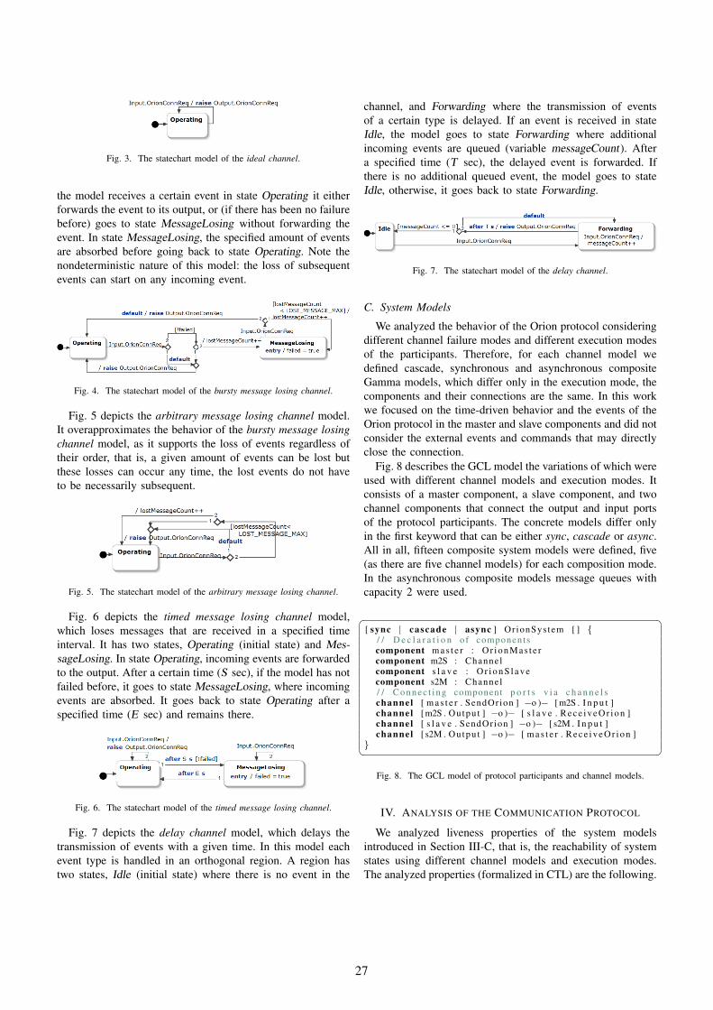
Fig. 3. The statechart model of the ideal channel.
the model receives a certain event in state Operating it eitherforwards the event to its output, or (if there has been no failurebefore) goes to state MessageLosing without forwarding theevent. In state MessageLosing, the specified amount of eventsare absorbed before going back to state Operating. Note thenondeterministic nature of this model: the loss of subsequentevents can start on any incoming event.
Fig. 4. The statechart model of the bursty message losing channel.
Fig. 5 depicts the arbitrary message losing channel model.It overapproximates the behavior of the bursty message losingchannel model, as it supports the loss of events regardless oftheir order, that is, a given amount of events can be lost butthese losses can occur any time, the lost events do not haveto be necessarily subsequent.
Fig. 5. The statechart model of the arbitrary message losing channel.
Fig. 6 depicts the timed message losing channel model,which loses messages that are received in a specified timeinterval. It has two states, Operating (initial state) and Mes-sageLosing. In state Operating, incoming events are forwardedto the output. After a certain time (S sec), if the model has notfailed before, it goes to state MessageLosing, where incomingevents are absorbed. It goes back to state Operating after aspecified time (E sec) and remains there.
Fig. 6. The statechart model of the timed message losing channel.
Fig. 7 depicts the delay channel model, which delays thetransmission of events with a given time. In this model eachevent type is handled in an orthogonal region. A region hastwo states, Idle (initial state) where there is no event in the
channel, and Forwarding where the transmission of eventsof a certain type is delayed. If an event is received in stateIdle, the model goes to state Forwarding where additionalincoming events are queued (variable messageCount). Aftera specified time (T sec), the delayed event is forwarded. Ifthere is no additional queued event, the model goes to stateIdle, otherwise, it goes back to state Forwarding.
Fig. 7. The statechart model of the delay channel.
C. System Models
We analyzed the behavior of the Orion protocol consideringdifferent channel failure modes and different execution modesof the participants. Therefore, for each channel model wedefined cascade, synchronous and asynchronous compositeGamma models, which differ only in the execution mode, thecomponents and their connections are the same. In this workwe focused on the time-driven behavior and the events of theOrion protocol in the master and slave components and did notconsider the external events and commands that may directlyclose the connection.
Fig. 8 describes the GCL model the variations of which wereused with different channel models and execution modes. Itconsists of a master component, a slave component, and twochannel components that connect the output and input portsof the protocol participants. The concrete models differ onlyin the first keyword that can be either sync, cascade or async.All in all, fifteen composite system models were defined, five(as there are five channel models) for each composition mode.In the asynchronous composite models message queues withcapacity 2 were used.
� �[ sync | cascade | async ] Or ionSys tem [ ] {
/ / D e c l a r a t i o n o f componentscomponent m a s t e r : Or io nMas t e rcomponent m2S : Channelcomponent s l a v e : O r i o n S l a v ecomponent s2M : Channel/ / C o n n e c t i n g component p o r t s v i a c h a n n e l schannel [ m a s t e r . SendOrion ] −o )− [m2S . I n p u t ]channel [ m2S . Outpu t ] −o )− [ s l a v e . R e c e i v e O r i o n ]channel [ s l a v e . SendOrion ] −o )− [ s2M . I n p u t ]channel [ s2M . Outpu t ] −o )− [ m a s t e r . R e c e i v e O r i o n ]
}� �Fig. 8. The GCL model of protocol participants and channel models.
IV. ANALYSIS OF THE COMMUNICATION PROTOCOL
We analyzed liveness properties of the system modelsintroduced in Section III-C, that is, the reachability of systemstates using different channel models and execution modes.The analyzed properties (formalized in CTL) are the following.
27

P1 The system can reach a state in which both themaster and the slave are in state Connected : EFmaster.Connected && slave.Connected.
P2 The system must eventually reach a state in which boththe master and the slave are in state Connected : AFmaster.Connected && slave.Connected.
P1 means the models do not contain fundamental faults. P2,as a robustness property means the protocol is always able torecover despite the specified failure mode of the channel.
According to the verification executed in Gamma, P1 holdsin the case of every system model introduced in Section III-C.The analysis results for P2 are shown in the following sections.
A. Synchronous Composition Mode
As the protocol has real-time timeouts, the fulfillment of theproperty depends on the execution frequency (indicated by f )of the system components in the case of each channel model.
In the case of the ideal channel model, f has to be higherthan 4/TConn for the property to hold due to the lock-step execution mode of the components: event transmissionbetween the master and the slave is delayed as events aretransmitted through separate channel components (the valuein the nominator refers to the number of components in thecomposite model). The timeout in state Connecting (both forthe master and the slave) is TConn sec. Therefore, eventOrionConnResp in response to OrionConnReq in the caseof the master, and event OrionConnConf in response toOrionConnReq in the case of the slave have to be receivedin lesser time to enable the reaching of state Connected.
The property holds in cases of both the burstyand arbitrary message losing channel models for allLOST MESSAGE MAX values between 1 and 9, if f ishigher than 4/TConn.
In the case of the timed message losing channel model, theproperty was checked for the following S and E values: 4 and9, 4 and 14, 4 and 19, 9 and 14, 9 and 19, 14 and 19 (so thatmultiples of parameters TReconn and TConn in the masterand slave models fall into these intervals). If f is higher than4/TConn, the property holds.
In the case of the delay message losing channel model, f,the T parameter of the channel and the TConn parameter inthe master and slave have to satisfy the following constraint:2/f + T < TConn/2. If this constraint is not satisfied, anexecution of the components can exist where the master andslave get desynchronized due to the late arrival of messagesand the Connected states are never reached at the same time.
B. Cascade Composition Mode
The cascade composition mode defines a sequential exe-cution semantics. Similarly to the synchronous compositionmode, the fulfillment of the analyzed property depends onthe execution frequency of components. The property canbe fulfilled in the case of every channel model, and in thiscomposition mode the execution frequencies can be lower.
In the case of the ideal channel, bursty-, arbitrary- andtimed message losing channel models, f has to be higher than
1/TConn for the property to hold, as components are executedin the following order: master, m2S, slave, s2M. Therefore,events from the master to the slave and from the slave to themaster can be transmitted in a single execution cycle.
In the case of the delay message losing channel model, f,the T and the TConn parameters have to satisfy the followingconstraint: 1/f + T < TConn/2.
C. Asynchronous Composition ModeIn the case of the asynchronous composition mode, there is
no guarantee on the execution frequency of the componentsof the composite model. Therefore, in the case of any channelmodel, it is possible to delay the execution of either the masteror slave component in state Connecting until the timeoutis reached (TConn sec). Thus, the property does not holdregardless of the defined channel models. To examine thisproblem, we introduced constraints on the execution frequencyof the components in the formal models. We observed that ifthe execution frequencies of the components are in the orderf(master) < f(m2S) < f(slave) < f(s2M), and are higherthan 4/TConn in the cases of the first four channel models,or the 2/f + T < TConn/2 constraint holds in the case of thedelay channel model, the property holds.
V. CONCLUSION
We proposed a verification approach for communicationprotocols using Gamma in the context of Orion, an industrialmaster-slave communication protocol. We defined multiplechannel models describing loss of events and delay of eventsfailure modes. Using model checking, we verified whether thesystem 1) might eventually and 2) must eventually reach a statein which both the master and slave are in state Connected.
In the future we plan to investigate the composition of chan-nel models in a single GCL component where the operatingchannel model is selected by a selector component. This way,both the model construction and the analysis phases could besimplified as the number of resulting system models woulddecrease to three. We also aim to introduce full support forexecution frequency constraints in asynchronous components.
Acknowledgment Supported by the European Union, co-financed by theEuropean Social Fund (EFOP-3.6.2-16-2017-00013) and the UNKP-19-3 NewNational Excellence Program of the Ministry for Innovation and Technology.
REFERENCES
[1] D. Harel, “Statecharts: A visual formalism for complex systems,” Sci.Comput. Program., vol. 8, no. 3, pp. 231–274, Jun. 1987.
[2] V. Molnar, B. Graics, A. Voros, I. Majzik, and D. Varro, “The GammaStatechart Composition Framework,” in 40th International Conference onSoftware Engineering (ICSE 2018). Gothenburg, Sweden: ACM, 2018.
[3] G. Behrmann, A. David, K. G. Larsen, J. Hakansson, P. Pettersson, W. Yi,and M. Hendriks, “Uppaal 4.0,” 2006.
[4] B. Graics and V. Molnar, “Mix-and-match composition in the GammaFramework,” in 25th Minisymposium, Department of Measurement andInformation Systems, Budapest, Hungary, January 2018.
[5] B. Graics, “Documentation of the Gamma Statechart CompositionFramework,” Budapest Univ. of Technology and Economics, Dept. ofMeasurement and Information Systems, Tech. Rep., 2016. [Online].Available: https://inf.mit.bme.hu/en/gamma/
[6] S. Procter and P. Feiler, “The AADL error library: An operationalizedtaxonomy of system errors,” Ada Lett., vol. 39, no. 1, p. 6370, Jan.2020. [Online]. Available: https://doi.org/10.1145/3379106.3379113
28

Abstraction-Based Model Checkingof Linear Temporal Properties
Milan Mondok, Andras VorosBudapest University of Technology and Economics
Department of Measurement and Information SystemsEmail: [email protected], [email protected]
Abstract—Even though the expressiveness of linear temporallogic (LTL) supports engineering application, model checkingof such properties is a computationally complex task and statespace explosion often hinders successful verification. LTL modelchecking consists of constructing automata from the propertyand the system, generating the synchronous product of the twoautomata and checking its language emptiness. We propose anovel LTL model checking algorithm that uses abstraction totackle the challenge of state space explosion. This algorithmcombines the advantages of two commonly used model checkingapproaches, counterexample-guided abstraction refinement andautomata theoretic LTL model checking. The main challenge incombining these is the refinement of ”lasso”-shaped counterex-amples, for which task we propose a novel refinement strategybased on interpolation.
I. INTRODUCTION
Linear temporal logic (LTL) specifications are particularlyexpressive and thus easy to use for engineers, but LTL modelchecking is a computationally expensive task. An efficient andcommonly used linear temporal logic verification algorithm isbased on automata theory. It consists of constructing automatafrom the property and the system, generating the synchronousproduct of the two automata and checking its language empti-ness. This reduces the LTL model checking task to productcalculation and language emptiness checking, which can beefficiently computed on Buchi automata, but the problem ofstate space explosion still hinders verification.
As the number of state variables in a system increases,the system’s state space grows at least exponentially, whichmakes the exploration resource-intensive. Several approacheswere developed to tackle the challenge of state space explo-sion. Counterexample-guided abstraction refinement checks asimplified model instead of the original problem, iterativelyadding more detail until the verification task can be decided.Abstraction-based solutions proved efficient in reachabilityanalysis, but have not been elaborated in the domain of LTLmodel checking yet.
We propose a novel LTL model checking algorithm thatperforms automata theoretic model checking on an iterativelyrefined abstract model. The abstraction is refined using a novelalgorithm based on interpolation.
Our approach is similar to the one described by Zhao Duanet al. in [4]. As an optimization, they limit the scope of the ver-ification to terminable programs and define an alternate versionof LTL that is interpreted over finite paths. These alternate LTL
formulas can be expressed using deterministic finite automata,which makes their verification computationally less demandingthan regular LTL model checking.
II. BACKGROUND
We use the following notation [6] from first-order logic(FOL) throughout our paper. Given a set of variables V =
{v1, v2, ...} let V ′ = {v′1, v′2, ...} and V 〈i〉 = {v〈i〉1 , v〈i〉2 , ...}
represent the primed and indexed version of the variables. Weuse V ′ to refer to successor states and V 〈i〉 for paths. Givenan expression ϕ over V ∪ V ′, let ϕ〈i〉 denote the indexedexpression obtained by replacing V and V ′ with V 〈i〉 andV 〈i+1〉 respectively in ϕ.
A. Control flow automata
In our work we describe programs using Control flowautomata (CFA) [6]. We define a Control flow automaton asa 4-tuple 〈V,L, l0, E〉, where:• V = {v1, v2, ..., vk} is the set of variables. Each variablevi has an associated domain Dvi ;
• L is the set of control locations, which model the programcounter;
• l0 ∈ L is the initial location;• E ⊆ L × Ops × L, where op ∈ Ops are FOL formulas
over V and V ′, is a set of directed edges representing theoperations that are executed when control flows from thesource location to the target.
A concrete state (l, c) is a pair of a location l ∈ Land an interpretation c ∈ Dv0 × ... × Dvn that assigns avalue c(v) = d ∈ Dv to each variable v ∈ V of itsdomain Dv . The set of initial states is {(l, c)|l = l0} anda transition exists between states (l, c) and (l′, c′) if an edge(l, op, l′) ∈ E exists with (c, c′) |= op. A concrete path is afinite, alternating sequence of concrete states and operationsσ = ((l1, c1), op1, ..., opn−1, (ln, cn)) if (li, opi, li+1) ∈ E forevery 1 ≤ i < n and (c
〈1〉1 , c
〈2〉2 , ..., c
〈n〉n ) |= ∧
1≤i<n op〈i〉i , i.e.,
there is a sequence of edges starting from the initial locationand the interpretations satisfy the semantics of the operations.
B. Counterexample-guided abstraction refinement
Counterexample-guided abstraction refinement (CEGAR)[2] [6] aims to tackle the problem of state space explosion byperforming the verification task on a simpler, abstract model.The abstract model is an overapproximation of the concrete
29

model: it contains all behaviours of the concrete model, butcan contain additional behaviour as well. Such models aresufficient to prove the absence of counterexamples but cancontain false positives, meaning that the counterexamples inthe abstract models have to undergo further analysis.
The core of the CEGAR algorithm is the CEGAR-loop,which consists of two components, the abstractor and therefiner. The task of the abstractor is to calculate the abstractstate space based on the current precision and to search forcounterexamples, while the task of the refiner is to verifythe concretizability of the abstract counterexample and refinethe precision accordingly. The loop can only be left in twoscenarios, either if the abstractor finds no counterexamples, orif the refiner finds that an abstract counterexample is feasible.
In Boolean predicate abstraction [6], an abstract state s ∈ Sin the set of abstract states is a Boolean combination of FOLpredicates. A precision π ∈ Π is a set of FOL predicatesthat are currently tracked by the algorithm. For example, ifthe current precision π contains two predicates, (x < 0) and(x < 1), then true, x < 0 or !(x < 0) ∧ x < 1 are examplesof possible abstract states.
The result of the transfer function [6] T (s, op, π) is thestrongest Boolean combination of predicates in the precisionthat is entailed by the source state s and the operation op.This can be calculated by assigning a fresh propositionalvariable vi to each predicate pi ∈ π and enumerating allsatisfying assignments of the variables vi in the formulas∧ op∧∧pi∈π(vi ↔ p′i). For each assignment, a conjunctionof predicates is formed by taking predicates with positive vari-ables and the negations of predicates with negative variables.The disjunction of all such conjunctions is the successor states′.
Locations of the CFA are tracked explicitly. Abstract statesSL = L × S are pairs of a location l ∈ L and a states ∈ S. The transfer function extended with locations isTL((l, s), π) = {(l′, s′)|(l, op, l′) ∈ E, s′ ∈ T (s, op, π)}, i.e.,(l′, s′) is a successor of (l, s) if there is an edge between land l′ with op and s′ is a successor of s with respect to theinner transfer function T .
An abstract path σ = ((l1, s1), op1, ..., opn−1, (ln, sn))is an alternating sequence of abstract states and operations.An abstract path is feasible if a corresponding concretepath ((l1, c1), op1, ..., opn−1, (ln, cn)) exists, where each ci ismapped to si.
The abstractor explores the abstract state space using asearch strategy (such as DFS of BFS) looking for counterex-amples, i.e., abstract paths that start in the initial state andend in an error state. The exploration starts in the abstract state(l0, true). When visiting a state, all of its unvisited successorswith respect to the transfer function TL are visited by thesearch. The search can be optimized by not visiting coveredsuccessors, i.e. abstract states (lc, sc), for which an alreadyvisited (lv, sv) exists such that lc = lv and (sc ⇒ sv). Ifall reachable states were visited and no counterexample wasfound, then the model is safe, however, if a counterexamplewas found the refiner needs to check its validity.
The refinement [6] happens as follows. The input is apath σ = ((l1, s1), op1, (l2, s2), op2, ..., opn−1, (ln, sn)) andthe current precision π. First, the feasibility of the pathis decided by querying an SMT solver with the formulas〈1〉1 ∧ op〈1〉1 ∧ s〈2〉2 ∧ op〈2〉2 ∧ ... ∧ op〈n−1〉n−1 ∧ s〈n〉n . If this
formula is satisfiable, then the model is unsafe and a satisfyingassignment to this formula is returned as the counterexample.Otherwise, an interpolant is calculated from the infeasible pathσ that holds information for the further steps of refinement.
A Craig interpolant [7] for a mutually inconsistent pairof formulas (A,B) is a formula that is (1) implied by A,(2) inconsistent with B, and (3) expressed over the commonvariables of A and B.
A binary interpolant for an infeasible path σ can be calcu-lated by defining A ≡ s
〈1〉1 ∧ op〈1〉1 ∧ ... ∧ op〈i−1〉i−1 ∧ s〈i〉i and
B ≡ op〈i〉i ∧ s〈i+1〉i+1 , where i corresponds to the longest prefix
of σ that is still feasible. The refined precision returned is theunion of π and the new predicate that is obtained by replacingthe variables V 〈i〉 with V in this interpolant.
C. Automata theoretic LTL model checking
Kripke structures, LTL expressions and Buchi automata canall be used to characterize ω-regular languages [10]. As LTLexpressions can only characterize a strict subset of ω-regularlanguages, while every ω-regular language can be recognizedby a Buchi automaton, all LTL-expressions can be transformedto equivalent Buchi automata, for example using the algorithmof Gerth et al [5].
We regard the state space of the model as a Kripke structureM . Given an LTL-formula ϕ let L(M) and L(ϕ) denotethe language that the Kripke structure can produce and thelanguage that the LTL-formula specifies. The LTL modelchecking problem [3] can now be restated as follows: is theset of provided behaviours a subset of the valid behaviours,i.e., does L(M) ⊆ L(ϕ) hold?
An equivalent formalization is L(M) ∩ L(ϕ)?= ∅, where
L(ϕ) is the complement of the language L(ϕ). Complemen-tation is computationally hard, but it can avoided in case ofLTL model checking by utilizing that the complement of thelanguage of an LTL-formula is the language of the negatedformula: L(ϕ) ≡ L(¬ϕ). This allows the model checkingproblem to be reduced to language intersection and languageemptiness, both of which can be efficiently computed on Buchiautomata.
A possible way of checking the language emptiness of aBuchi automaton is checking whether at least one stronglyconnected component (SCC) that contains an accepting stateis reachable from the initial state. If such an SCC is reachable,then the Buchi automaton contains at least one run thatcontains an accepting state infinitely many times, fulfilling theacceptance condition of Buchi automata. Tarjan’s algorithm [9]identifies SCCs using a single depth-first search (DFS) andclever indexing. Algorithms based on Nested DFS [8] offera different approach. These algorithms usually conduct twodepth-first searches, the former one to find and sort accepting
30

states, and the latter one to find cycles that contain acceptingstates.
III. OVERVIEW OF THE APPROACH
LTL model checkers have always struggled with perfor-mance. We propose to use counterexample-guided abstractionrefinement in LTL model checking. The key idea of our ap-proach (Fig. 1) is that we conduct the automata theoretic LTLmodel checking on abstract models that we iteratively refineto the required precision using the the CEGAR algorithm.
The algorithm can work with various abstract domains, suchas explicit value abstraction [1], predicate abstraction, or evena mix of the two. The appropriate abstraction method can onlybe selected based on the desired application domain. In thispaper, we present the algorithm using predicate abstraction, avariant more suited for reactive systems as variables in suchsystems usually only get assigned a relatively small subset oftheir domains as values.
The algorithm has the following steps:1) The requirement specification is given in the form of an
LTL-formula ϕ. Negate this formula and transform it toan equivalent Buchi automaton S;
2) Apply abstraction to the concrete model with the currentprecision, calculate the abstract state space and representit with an automaton M ;
3) Calculate the synchronous product of the two automataS × M . During each step of the product the modelautomaton steps first, then the specification automatonsteps based on the target state of the model automaton.
4) Check the language emptiness of the product automatonS ×M ;• If the language of the product is empty, then the
model meets the correctness specification as nocounterexamples were found;
• If a counterexample is found in the abstract statespace, then verify whether it is feasible in theconcrete state space as well;– A feasible counterexample means that the model
does not meet the correctness specification (i.e.is unsafe), as we found a contradicting trace;
– If the counterexample isn’t feasible in the con-crete system (i.e. spurious), then refine the pre-cision and jump to step 2.
When using a suitable language emptiness checking al-gorithm such as Nested DFS [8], the tasks of state spacegeneration, calculation of the product automaton and languageemptiness checking can be conducted together, which canresult in a significant increase in performance. If these threetasks are carried out at the same time, then the model checkingis said to happen ”on-the-fly”.
IV. REFINEMENT
In this section we present a novel refinement method forpredicate abstraction. The algorithm searches for counterex-amples that have a ”lasso”-like form. The first part of the
LTLtoBA¬φ
Abstractor
S×M
M
S
concretemodel
L(S×M)?=∅
Refiner
✓true
abstractcounterexample
concretecounterexample
refinedprecision
Xinitialprecision
Fig. 1. Overview of CEGAR-based LTL model checking.
counterexample is a path leading to an accepting state and thesecond part is a cycle which starts and ends in said acceptingstate. If such a counterexample is found, then an acceptingrun is possible, because by repeatedly traversing the cycle, anaccepting state can be explored infinitely many times, fulfillingthe Buchi acceptance condition.
The CEGAR algorithm is usually used for reachabilitychecking, where counterexamples are abstract paths leadingfrom the initial state to an error state. When verifying thesecounterexamples the only thing that needs to be checked iswhether such a path exists in the concrete model, whose statesand transitions all correspond to the states and transitions ofthe abstract path. However, the fulfillment of this condition isrequired, but not enough, when analysing a cycle. A path thatis not a cycle in the concrete model might appear as one inthe abstract model.
We developed a novel counterexample refinementstrategy that is capable of handling ”lasso”-likecounterexamples. The input is an abstract pathσ = ((l1, s1), op1, (l2, s2), op2, ..., opn−1, (ln, sn)) andan integer 1 ≤ cycle ≤ n that is the index of the initial stateof the cycle, i.e. the recurrent accepting state (scycle = sn).The path is first fed to the traditional CEGAR refinementalgorithm presented in Section II-B. Based on the result ofthis algorithm, we have two options. If the algorithm findsthat the path isn’t traversable and returns a refined precision,then we simply return this refined precision. However, if thealgorithm finds that the path is traversable, then we conductfurther analysis to decide whether it is traversable in sucha way that the initial and the end state of the cycle are thesame concrete states.
Control locations are tracked explicitly during state spaceexploration, thus deciding whether two concrete states thatbelong to the same abstract state are identical can be doneby comparing their data values (i.e. the values assignedto the variables in them). We construct a constraint B ≡∧v∈V v
〈cycle〉 = v〈n〉, which expresses that each variablehas the same value in the initial and end state of the cycle,i.e. they are the same concrete states. We also constructthe same formula that the refinement algorithm in II-B usedto verify traversability, A ≡ s
〈1〉1 ∧ op〈1〉1 ∧ ... ∧ s〈cycle〉cycle ∧
op〈cycle〉cycle ∧ ... ∧ op
〈n−1〉n−1 ∧ s〈n〉n . By querying an SMT solver
with the conjuntion of these two formulas, i.e., A ∧ B, we
31

T !(x<=0) !(x<=0)x'=1 x<5∧x'=x
x'=x+1�1 ,�2 �4 �3Text
Fig. 2. Example of an abstract counterexample.
verify whether the counterexample is feasible. If this formulais satisfiable then the model does not meet the requirementspecification (i.e. is unsafe) and a satisfying assignment isreturned as counterexample. If the formula isn’t satisfiable (i.e.is spurious), then we refine the precision by calculating aninterpolant based on this formula.
Algorithm 1 Lasso refinementInput: σ: abstract path, cycle: initial index of cycleOutput: (unsafe or spurious , π′)
1: procedure lasso refine(σ, cycle)2: res := refine(σ)3: if res is spurious then return res4: else5: A ≡ s〈1〉1 ∧ op
〈1〉1 ∧ ... ∧ op
〈n−1〉n−1 ∧ s
〈n〉n
6: B ≡ ∧v∈V v
〈cycle〉 = v〈n〉
7: if A ∧B is feasible then return (unsafe, π)8: else9: I ← get interpolant for (A, B)
10: η ← get satisfying assignment for A11: π′ ← create predicate from I:12: replace all v〈n〉 ∈ I with v13: replace all v〈cycle〉 ∈ I with η(v〈cycle〉)14: return (spurious, π ∪ π′)
To refine the precision we obtain an interpolant I for Aand B. This interpolant is interpreted over V 〈cycle〉 and V 〈n〉,let’s denote this with I(v
〈cycle〉1 , ..., v
〈cycle〉k , v
〈n〉1 , ..., v
〈n〉k ). We
also query the SMT solver for a satisfying assignment ηto the formula A, which describes a concrete path σ =((l1, c1), op1, ..., opn−1, (ln, cn)), where ccycle 6= cn. To en-sure that the spurious counterexample described by η isn’tfound again during later explorations of the abstract statespace, we need to extend our precision with a new predicateπ′(v1, ..., vk) that evaluates to false in ccycle and to true incn (or vice versa), so that ccycle and cn get mapped to differ-ent abstract states. Formally, π′(η(v
〈cycle〉1 ), ..., η(v
〈cycle〉k )) =
false and π′(η(v〈n〉1 ), ..., η(v
〈n〉k )) = true. To construct
the predicate π′ from the interpolant I , we replace thevariables V 〈n〉 with V , and V 〈cycle〉 with values thatare assigned to them by η. Formally, π′(v1, ..., vk) :=
I(η(v〈cycle〉1 ), ..., η(v
〈cycle〉k ), v1, ..., vk).
If we evaluate π′(η(v〈n〉1 ), ..., η(v
〈n〉k )), i.e. π′ in cn, we
get I(η(v〈cycle〉1 ), ..., η(v
〈cycle〉k ), η(v
〈n〉1 ), ..., η(v
〈n〉k )), which is
true, because of the first property of Craig interpolants(A → I), from which it follows that if an assignment ηsatisfies A, then it also satisfies I .
Evaluating π′ in ccycle however, results inI(η(v
〈cycle〉1 ), ..., η(v
〈cycle〉k ), η(v
〈cycle〉1 ), ..., η(v
〈cycle〉k )),
which is false. In this case the variables V 〈cycle〉 areassigned the same values as their counterparts V 〈n〉, whichmeans that B is true. It follows that I in this case is false,because of the second property of Craig interpolants (I ∧ Bis unsatisfiable),
We demonstrate the refinement process on the abstract coun-terexample in Fig. 2. The white rectangles represent abstractstates with the applying predicates displayed inside them, thearrows represent transitions, the precision only contains onepredicate, (x ≤ 0). The value of cycle and n is 2 and 4,respectively. We construct the following formulas based onthis path:
A ≡ true ∧ x〈2〉=1 ∧ !(x〈2〉≤0) ∧ x〈2〉<5∧x〈3〉=x〈2〉 ∧!(x〈3〉≤0) ∧ x〈4〉=x〈3〉+1 ∧ !(x〈4〉≤0)
B ≡ x〈2〉=x〈4〉
By querying an SMT solver with the formula A∧B we findthat the counterexample in spurious, as A∧B isn’t satisfiable.The solver returns the interpolant I ≡ x〈2〉 < x〈4〉 (note thatthis is only one of the possible interpolants). We request asatisfying assignment for A from the solver, and construct apredicate from I by replacing x〈4〉 with x and x〈2〉 with 1(the value that is assigned to it in the satisfying assignment).Finally, we return that the counterexample is spurious, accom-panied by the refined precision (x ≤ 0), (1 < x).
V. CONCLUSION
In our paper we examined LTL model checking and pro-posed a novel algorithm, which combines the advantages ofcounterexample-guided abstraction refinement and automatatheoretic LTL model checking. We also proposed a novelrefinement method for predicate abstraction. We implementedour algorithm in the Theta framework [11], but chose to omitexperimental evaluation from this paper due to the lack ofspace.
REFERENCES
[1] Dirk Beyer and Stefan Lowe. Explicit-state software model checkingbased on cegar and interpolation. 2013.
[2] Edmund Clarke, Orna Grumberg, Somesh Jha, Yuan Lu, and HelmutVeith. Counterexample-guided abstraction refinement for symbolicmodel checking. 2003.
[3] Edmund M. Clarke, Jr., Orna Grumberg, and Doron A. Peled. ModelChecking. MIT Press, 1999.
[4] Zhao Duan, Cong Tian, and Zhenhua Duan. Verifying temporalproperties of c programs via lazy abstraction. 2017.
[5] Rob Gerth, Doron Peled, Moshe Y. Vardi, and Pierre Wolper. Simpleon-the-fly automatic verification of linear temporal logic. 1996.
[6] Akos Hajdu and Zoltan Micskei. Efficient strategies for cegar-basedmodel checking. 2019.
[7] Kenneth McMillan. Applications of craig interpolation to model check-ing. 2005.
[8] Stefan Schwoon and Javier Esparza. A note on on-the-fly verificationalgorithms. 2005.
[9] Robert Tarjan. Depth first search and linear graph algorithms. 1972.[10] Wolfgang Thomas. Handbook of theoretical computer science (vol. b).
chapter Automata on Infinite Objects. 1990.[11] Tamas Toth, Akos Hajdu, Andras Voros, Zoltan Micskei, and Istvan
Majzik. Theta: a framework for abstraction refinement-based modelchecking. 2017.
32

Incremental view maintenance in graph databases:A case study in Neo4j
Marton Elekes, Gabor SzarnyasBudapest University of Technology and Economics
Department of Measurement and Information SystemsBudapest, Hungary
Email: {elekes, szarnyas}@mit.bme.hu
Abstract—With the increasing amount of densely connecteddata sets, graph analysis has become an integral part of dataprocessing pipelines. Therefore, the last decade saw the emer-gence of numerous dedicated graph analytical systems along withspecialized graph database management systems. Traditionally,graph analytical tools targeted global fixed-point computations,while graph databases focused on simpler transactional readoperations such as retrieving the neighbours of a node. However,recent applications of graph processing (such as financial frauddetection and serving personalized recommendations) often ne-cessitate a mix of the two workload profiles. Following this trend,the 2018 Transformation Tool Contest (an annual competitionfor graph transformation tools) presented a case study thatrequires participants to compute complex graph queries definedon a continuously changing social network graph. The solutionsare assessed based on their scalability and query reevaluationtime, therefore, solutions are encouraged to incrementalize theirimplementations. This paper demonstrates a solution in thepopular Neo4j graph database using several incrementalizationtechniques and compares them against the reference implemen-tation of the case study.
Fig. 1: Graph schema of the case study.
I. INTRODUCTION
We start by describing the “Social Media” case study ofthe 2018 Transformation Tool Contest [5]. This case study isdefined using a familiar social network-like data model (Fig. 1)consisting of Users and their Submissions. These submissionsform a tree where the root node is a Post and the rest ofthe nodes are Comments. Users can like Comments and formfriends relations with each other. Additionally, Comments havea direct pointer rootPost to the root Post to allow quicklookups. Fig. 2a shows an example graph with two Posts (p1,p2), three Comments (c1, c2, c3) and four Users (u1, . . . ,u4). Solutions are required to compute two queries:Q1: influential posts. Assign a score to each Post, definedas 10 times the number of their (direct or indirect) Comments
(a) Initial graph and scores. Comment c2 has two components: c2/aconsists of User u1, while c2/b consists of Users u3 and u4. Itstotal score is the sum of the component sizes, i.e. 12 + 22 = 5.
(b) Graph after performing an update that inserted six entities: (1) afriends edge between Users u1 and u4, (2) a likes edge fromUser u2 to Comment c2, (3) a Comment node c4 with (4) anoutgoing rootPost edge to Post p1, (5) an outgoing commentededge to Comment c1, and (6) an incoming likes edge from Useru4. The changes have increased the score of Post p1 and resultedin Comment c2 having a single component of size 4, thereforereceiving a score of 42 = 16. Comment c4 getting a score of 12 = 1.
Fig. 2: Example graphs: initial and updated versions.
plus the number of Users liking those Comments. Return thetop 3 Posts according to their score.Q2: influential comments. Assign a score to each Comment,based on the friendships of the Users who like that Comment.Based on the graph formed by the User nodes and their friendsedges, for every comment we define an induced subgraphwhich contains the Users who like the Comment and theirfriends edges. The subgraph contains connected components,
33

EnumPaths EnumPaths Reachability MatComp MatComp GraphAlgo GraphAlgo MatCompSubgraph Subgraph FixedPoint PathOp EdgeFilter GraphAlgo
(very slow) (incompatible) ●
initi
alev
alua
tion enumerate paths
materialize subgraph (edges/labels) E reachability (shortestPath) Ereachability+dynamic labels (APOC lib.) fixed-point calculation (APOC library) materialize subgraph components Graph Algorithms library
upda
te reevaluationn/a n/a
maintain component dirty flag for Comments
TABLE I: Comparison of strategies for Q2 regarding the techniques (language features and libraries) used in each strategy.Strategies in bold are described in more detail. Notation – : the technique is used by the strategy, E: incompatible strategies.“MatComp” strategies are denoted with ◻, while “GraphAlgo” strategies are denoted with ×.
i.e. groups of users who know each other directly or viafriends. The score is defined as the sum of squared componentsizes. Finally, the top 3 Comments should be returned.Updating the graph. After the query execution on the initialgraph the case study requires solutions to perform a numberof updates on the graph while maintaining the results of thequeries. Fig. 2 shows the initial graph and the updated graphwith the scores for Q1 and Q2.Neo4j. Neo4j is a graph database management system usingthe property graph data model. Such graphs consist of la-belled entities, i.e. nodes and edges, which can be describedwith properties encoded as key-value pairs. Neo4j uses theCypher query language [2] which offers both read and updateconstructs [3]. While the main focus of Neo4j is to run graphqueries, it also supports graph analytical algorithms with therecently released Graph Algorithms library [7].
II. APPROACH
Q1 Batch. Q1 can be expressed with the Cypher query inListing 1. The Cypher language uses node labels (e.g. Post,Comment, User), edge types (e.g. ROOT POST, LIKES),node and edges properties to express graph patterns. Thequery matches every node with label Post, then all its com-ments via the rootPost edges, then the Users via the likesedges. OPTIONAL MATCH denotes an optional pattern, wherevariables are filled with NULL values if there is no match.RETURN can be also used to group and aggregate. The resultsare grouped by the id and timestamp properties of the Posts,aggregated, then the top 3 scores are returned. The aggregationcounts the likes using the number of Users (a User canlike more Comments), and counts the number of Comments(DISTINCT is used to remove duplicate Comments).
1 MATCH (p:Post)2 OPTIONAL MATCH (p)<-[:ROOT_POST]-(c:Comment)3 OPTIONAL MATCH (c)<-[:LIKES]-(u:User)4 RETURN p.id AS id,5 10*count(DISTINCT c)+count(u) AS score,6 p.timestamp AS timestamp7 ORDER BY score DESC, timestamp DESC LIMIT 3
Listing 1: Q1 Batch.
Q1 Incremental. To incrementally evaluate Q1, we initiallycompute the score for each Post as previously and store it in
score property (Listing 2). Based on this property the currenttop 3 scores can be computed using Listing 3. The scoreproperty is indexed to improve lookup times.
For every batch of updates Alg. 1 is executed to insert newelements and update the score property, then Listing 3 is usedto get the top 3.
1 MATCH (p:Post)2 OPTIONAL MATCH (p)<-[:ROOT_POST]-(c:Comment)3 OPTIONAL MATCH (c)<-[:LIKES]-(u:User)4 WITH p, 10*count(DISTINCT c)+count(u) AS score5 SET p.score = score
Listing 2: Q1 Incremental – initial evaluation.
1 MATCH (p:Post)2 WHERE p.score >= 0 // query hint to use index3 RETURN p.id AS id, p.score AS score,4 p.timestamp AS timestamp5 ORDER BY score DESC, timestamp DESC LIMIT 3
Listing 3: Q1 Incremental – get top 3 results.
Algorithm 1 Maintaining scores for Q11: procedure UPDATEQ1(updates)2: for all update ∈ updates do3: ADDNEWELEMENT(update) ▷ insert into the graph4: if update isPost then5: update.score← 0 ▷ init score for new Post6: else if update is ⟨Comment,Post⟩ then ▷ new Comment node7: ⟨ , rp⟩← update ▷ get the root Post8: rp.score← rp.score + 10 ▷ update score9: else if update is ⟨User,Comment⟩ then ▷ new likes edge
10: ⟨ , c⟩← update ▷ get Comment vertex of new edge11: rp ← ROOTPOST(c) ▷ navigate via rootPost12: rp.score← rp.score + 1 ▷ update score13: end if14: end for15: end procedure
Q2 Strategies. Table I compares the different strategies usedfor Q2 to find connected components in a subgraph and handleupdates. Fig. 3 shows a comparison of their runtime duringthe initial evaluation and after the updates. The EnumPathsstrategy finds the connected components by enumerating allpaths of friends edges between Users who like a comment
34

and filtering to ensure that every User on the path also likesthe Comment. The complexity of this operation is intractable,therefore this strategy is not feasible on larger graphs. Toonly enumerate valid paths in the subgraph, the edges of thesubgraph can be materialized for each subgraph, i.e. for eachComment (stored as an edge property). The combination ofthese techniques (EnumPaths Subgraph ) also exhibits poorscalability (later measurements show that it reaches the timelimit after graph size 8). This limitation could be resolvedby using a Cypher reachability query, but unfortunately suchqueries cannot perform filtering on properties (which is nec-essary to ensure we only enumerate valid paths).
To use reachability queries and avoid the costly enumerationof paths, MatComp FixedPoint strategy uses Neo4j’s APOClibrary1. It materializes subgraph components by converting◯ likesÐÐ→◯User Comment edges to ◯componentÐÐÐÐÐ→◯Comment Component and
◯userÐÐ→◯Component User edges where the Component node con-nects every User who knows each other directly or via friends.The conversion is executed for each component one by oneusing the fixed-point query execution mechanism of APOC.This strategy has the best performance, which is caused bythe use of reachability function and incremental maintenanceafter updates. Component materialization can be expressedwith pure Cypher queries using path operations (MatCompPathOp , which also has limited scalability due to the use ofpath enumeration.
GraphAlgo strategies (×) use functions provided by theNeo4j Graph Algorithms library2 [7] to find connected com-ponents in a subgraph conveniently. The library loads the sub-graph into an in-memory projected subgraph before runningthe computations. The initial runtimes of these solutions areworse than the runtime of MatComp FixedPoint. This can beattributed to the load phase, which is run for every subgraph,i.e. for every Comment.
Strategies can differ in the way they handle the updates: theycan fully reevaluate the queries or incrementally maintain theresults depending on the update. Repeated reevaluations takea significant amount of time, which causes the execution totime out. EnumPaths Subgraph strategy uses Comment-level incrementalization with dirty flags, but using path enu-merations limits its scalability. The incremental evaluation ofmaterialized components (◻) is implemented by merging thecomponents and maintaining their sizes and the scores. Theseupdates have the best performance. (The MatComp strategieswith worse initial runtime reaches the time limit.)Q2 Batch. Listing 4 shows the GraphAlgo solutionfor Q2 using Neo4j Graph Algorithms library. Thealgo.unionFind.stream function is used to find con-nected components of the subgraph given by the node labelsand edge types or Cypher queries. For each Comment, thefirst Cypher query in Lines 3–7 select Users who like theComment, the second query selects all friend edges as pairs
1https://neo4j.com/labs/apoc/2https://neo4j.com/docs/graph-algorithms/
1 MATCH (c:Comment)2 CALL algo.unionFind.stream(3 'MATCH (c:Comment)<-[:LIKES]-(u:User)4 WHERE id(c)=' + id(c) + '5 RETURN id(u) as id',6 'MATCH (u1:User)-[:FRIEND]->(u2:User)7 RETURN id(u1) as source, id(u2) as target',8 {graph: 'cypher'})9 YIELD setId
10 WITH c, setId, count(setId) AS cSize11 WITH c, cSize * cSize AS cSize_212 RETURN c.id AS id, sum(cSize_2) AS score, c.
timestamp13 ORDER BY score DESC, c.timestamp DESC LIMIT 314 UNION ALL15 MATCH (c:Comment)16 WHERE NOT (c)<-[:LIKES]-(:User)17 RETURN c.id AS id, 0 AS score, c.timestamp18 ORDER BY c.timestamp DESC LIMIT 3
Listing 4: Q2 batch using the Neo4j Graph Algorithms library.
●●
●●
●●
●
●
Initial Update
Q2
1 2 4 8 16 32 64 128 256 512 1024 1 2 4 8 16 32 64 128 256 512 1024
0.1
1
10
100
1000
Graph size
Exe
cutio
n tim
e [s
]
Technique
●
Enumerate paths on subgraph
Graph Algorithms + edge filter (batch)
Graph Algorithms library (batch)
Materialize components by fixed−point calculation
Materialize components by Graph Algorithms library
Materialize components by path operations
Fig. 3: Performance comparison of Q2 strategies. The symbolsdenoting techniques correspond to those shown in Table I.
of Users. The function returns the ID of the componentcontaining the User node. Lines 10–14 calculate the squaredsum of the component sizes and selects the top 3 scores. Thefunction is invoked only for Comments with likes. The top 3Comments without likes are enumerated by Lines 16–20.Q2 Incremental. The incremental solution in this section(MatComp FixedPoint) materializes the components of thesubgraph using fixed-point query execution of APOC library.To achieve this, the solution materializes subgraph edges asdynamically named labels (Listing 5) and finds reachablenodes using the APOC library (Listing 6). The incrementalevaluation is performed by merging the components andmaintaining their sizes and the scores (Listing 7).
III. EVALUATION
To evaluate the performance and scalability of our solution,we have used the benchmark framework of the case study [5].This executes the queries on graphs of increasing sizes asshown in Table II, then adds new elements to the graph, andmaintains the result using the queries. (Similar queries can beformulated for element removal.) As a performance baseline,
35
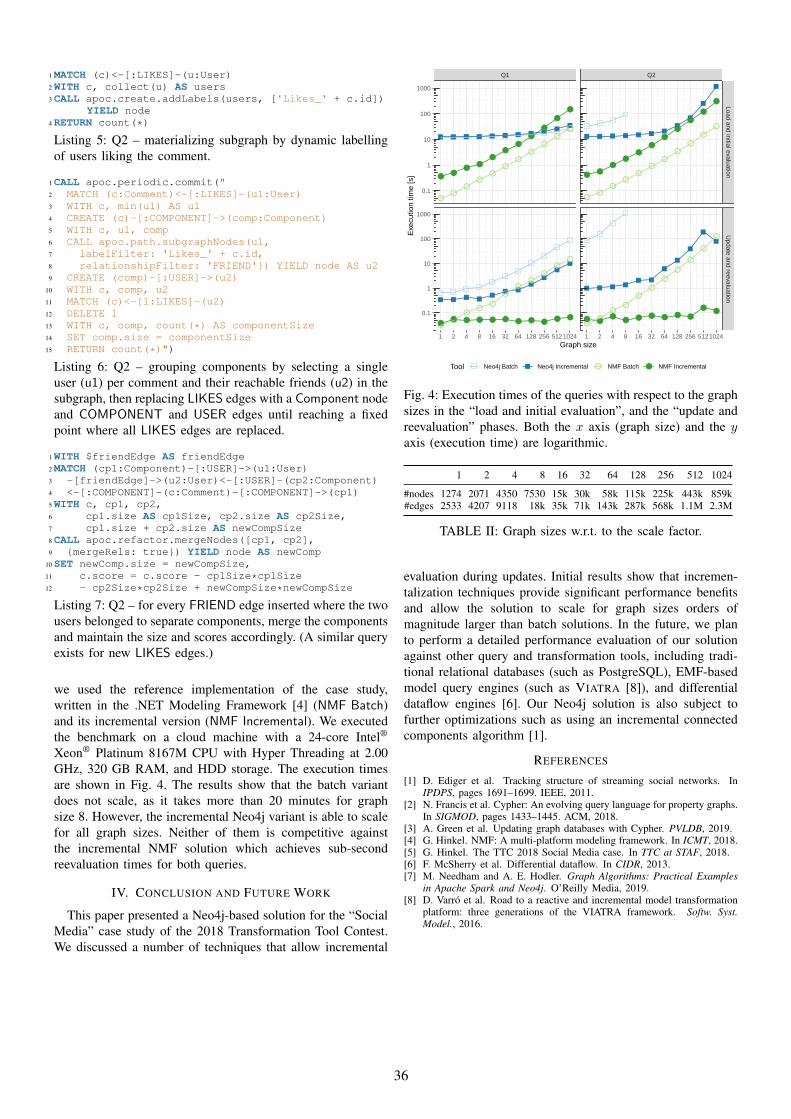
1 MATCH (c)<-[:LIKES]-(u:User)2 WITH c, collect(u) AS users3 CALL apoc.create.addLabels(users, ['Likes_' + c.id])
YIELD node4 RETURN count(*)
Listing 5: Q2 – materializing subgraph by dynamic labellingof users liking the comment.
1 CALL apoc.periodic.commit("2 MATCH (c:Comment)<-[:LIKES]-(u1:User)3 WITH c, min(u1) AS u14 CREATE (c)-[:COMPONENT]->(comp:Component)5 WITH c, u1, comp6 CALL apoc.path.subgraphNodes(u1,7 labelFilter: 'Likes_' + c.id,8 relationshipFilter: 'FRIEND'}) YIELD node AS u29 CREATE (comp)-[:USER]->(u2)
10 WITH c, comp, u211 MATCH (c)<-[l:LIKES]-(u2)12 DELETE l13 WITH c, comp, count(*) AS componentSize14 SET comp.size = componentSize15 RETURN count(*)")
Listing 6: Q2 – grouping components by selecting a singleuser (u1) per comment and their reachable friends (u2) in thesubgraph, then replacing LIKES edges with a Component nodeand COMPONENT and USER edges until reaching a fixedpoint where all LIKES edges are replaced.
1 WITH $friendEdge AS friendEdge2 MATCH (cp1:Component)-[:USER]->(u1:User)3 -[friendEdge]->(u2:User)<-[:USER]-(cp2:Component)4 <-[:COMPONENT]-(c:Comment)-[:COMPONENT]->(cp1)5 WITH c, cp1, cp2,6 cp1.size AS cp1Size, cp2.size AS cp2Size,7 cp1.size + cp2.size AS newCompSize8 CALL apoc.refactor.mergeNodes([cp1, cp2],9 {mergeRels: true}) YIELD node AS newComp
10 SET newComp.size = newCompSize,11 c.score = c.score - cp1Size*cp1Size12 - cp2Size*cp2Size + newCompSize*newCompSize
Listing 7: Q2 – for every FRIEND edge inserted where the twousers belonged to separate components, merge the componentsand maintain the size and scores accordingly. (A similar queryexists for new LIKES edges.)
we used the reference implementation of the case study,written in the .NET Modeling Framework [4] (NMF Batch)and its incremental version (NMF Incremental). We executedthe benchmark on a cloud machine with a 24-core Intel®
Xeon® Platinum 8167M CPU with Hyper Threading at 2.00GHz, 320 GB RAM, and HDD storage. The execution timesare shown in Fig. 4. The results show that the batch variantdoes not scale, as it takes more than 20 minutes for graphsize 8. However, the incremental Neo4j variant is able to scalefor all graph sizes. Neither of them is competitive againstthe incremental NMF solution which achieves sub-secondreevaluation times for both queries.
IV. CONCLUSION AND FUTURE WORK
This paper presented a Neo4j-based solution for the “SocialMedia” case study of the 2018 Transformation Tool Contest.We discussed a number of techniques that allow incremental
●●
●●
●●
●●
●●
●
●●
●●
●●
●●
●
●
●
●●
●●
●
●●
●●
●●
●● ● ● ● ● ● ● ● ● ●
●●
●●
●●
●●
●
●
●
●●
●●
●●
●●
●
●
●
●●
●●
●●
●
●
●
●
●
● ●●
● ● ● ● ● ●
● ●
Q1 Q2
Load and initial evaluationU
pdate and reevaluation
1 2 4 8 16 32 64 128 256 5121024 1 2 4 8 16 32 64 128 256 5121024
0.1
1
10
100
1000
0.1
1
10
100
1000
Graph size
Exe
cutio
n tim
e [s
]
Tool ● ●Neo4j Batch Neo4j Incremental NMF Batch NMF Incremental
Fig. 4: Execution times of the queries with respect to the graphsizes in the “load and initial evaluation”, and the “update andreevaluation” phases. Both the x axis (graph size) and the yaxis (execution time) are logarithmic.
1 2 4 8 16 32 64 128 256 512 1024
#nodes 1274 2071 4350 7530 15k 30k 58k 115k 225k 443k 859k#edges 2533 4207 9118 18k 35k 71k 143k 287k 568k 1.1M 2.3M
TABLE II: Graph sizes w.r.t. to the scale factor.
evaluation during updates. Initial results show that incremen-talization techniques provide significant performance benefitsand allow the solution to scale for graph sizes orders ofmagnitude larger than batch solutions. In the future, we planto perform a detailed performance evaluation of our solutionagainst other query and transformation tools, including tradi-tional relational databases (such as PostgreSQL), EMF-basedmodel query engines (such as VIATRA [8]), and differentialdataflow engines [6]. Our Neo4j solution is also subject tofurther optimizations such as using an incremental connectedcomponents algorithm [1].
REFERENCES
[1] D. Ediger et al. Tracking structure of streaming social networks. InIPDPS, pages 1691–1699. IEEE, 2011.
[2] N. Francis et al. Cypher: An evolving query language for property graphs.In SIGMOD, pages 1433–1445. ACM, 2018.
[3] A. Green et al. Updating graph databases with Cypher. PVLDB, 2019.[4] G. Hinkel. NMF: A multi-platform modeling framework. In ICMT, 2018.[5] G. Hinkel. The TTC 2018 Social Media case. In TTC at STAF, 2018.[6] F. McSherry et al. Differential dataflow. In CIDR, 2013.[7] M. Needham and A. E. Hodler. Graph Algorithms: Practical Examples
in Apache Spark and Neo4j. O’Reilly Media, 2019.[8] D. Varro et al. Road to a reactive and incremental model transformation
platform: three generations of the VIATRA framework. Softw. Syst.Model., 2016.
36

Continuous time modelling of autocatalyticchemical reaction dynamics from sporadic inputs
Edward De BrouwerESAT-STADIUS
KU LeuvenLeuven, Belgium
Adam AranyESAT-STADIUS
KU LeuvenLeuven, Belgium
Jaak SimmESAT-STADIUS
KU LeuvenLeuven, Belgium
Yves MoreauESAT-STADIUS
KU LeuvenLeuven, Belgium
Abstract—Real-world time series are usually sporadically ob-served when collected outside of rigorous scientific experiments.The sampling is irregular across time and across dimensions,which breaks the typical assumption of most recurrent networksand dynamical process models. In this work, we propose to useour GRU-ODE-Bayes [1], a recently proposed model that posits acontinuous latent process whose dynamics are driven by an ordi-nary differential equation parametrized with neural networks [2].We apply this framework in the estimation of reaction dynamicsfrom observational data. In particular, we show that our methodis able to learn unstable autocatalytic chemical reactions withinthe large class of reactions driven by the Brusselator dynamicalmodel [3], such as the Belousov–Zhabotinsky reaction in thepresence of very few sporadic observation points.
Index Terms—Neural Networks, Time Series, ODE, ChemicalReactions Dynamics
I. INTRODUCTION AND MOTIVATION
Scientific research produces large quantity of time seriesdata from various domains such as chemistry, astronomy,healthcare or climate science. Even though most statisticalmethods for analyzing this type of data assumes that signalsare measured systematically at fixed constant time intervals,this assumption is often not hold in practice.
Indeed, due to some practical contingencies, much real-world data is sporadic (i.e., the signals are sampled irregularlyand not all signals are measured each time). A typical exampleis patient measurements, which are taken when the patientcomes for a visit (e.g., sometimes skipping an appointment)
Edward De Brouwer is funded by a FWO-SB grant. Yves Moreau is fundedby (1) Research Council KU Leuven: C14/18/092 SymBioSys3; CELSA-HIDUCTION, (2) Innovative Medicines Initiative: MELLODY, (3) FlemishGovernment (ELIXIR Belgium, IWT, FWO 06260) and (4) Impulsfonds AI:VR 2019 2203 DOC.0318/1QUATER Kenniscentrum Data en Maatschappij.Computational resources and services used in this work were provided by theVSC (Flemish Supercomputer Center), funded by the Research Foundation- Flanders (FWO) and the Flemish Government – department EWI. We alsogratefully acknowledge the support of NVIDIA Corporation with the donationof the Titan Xp GPU used for this research. The research has also beensupported by the European Union, co-financed by the European Social Fund(EFOP-3.6.2-16-2017-00013, Thematic Fundamental Research CollaborationsGrounding Innovation in Informatics and Infocommunications).
and where not every measurement is taken at every visit.Another example would be running lab experiments spreadover several days when sensor errors can occur.
Modeling then becomes challenging as such data violatesthe main assumptions underlying traditional machine learn-ing methods (such as recurrent neural networks). The moststraightforward way to address this issue is to perform impu-tation, but this is often unsatisfactory as it results in biasedestimates.
Recently, the GRU-ODE-Bayes model [1] proposed a novelway to address this type of sporadic time series for forecastingand classification. Based on the seminal Neural-ODE idea[2], it proposes a filtering approach that posits a continuouslatent process that generates the observations. By framingthe dynamics as an ordinary differential equation (ODE)parametrized by neural networks, the model is able to modelcomplex dynamics and integrate it over arbitrary time inter-vals, therefore addressing the sporadicity issue in a naturalway. Furthermore, it was shown that the continuity prior wasproviding extra performance when the continuity assumption isverified in practice, such as in patients clinical data predictionor weather forecasting.
This continuity assumption is also valid in chemical reactiondynamics. Indeed, chemical reactions are intrinsically contin-uous and can most of the time be expressed analytically asODEs. However, reactions in multiple component mixturesare very complex and the true dynamic is often unknown.In this case, chemists try to approximate the true dynamicof the process by running some temporal experiments andlearning the underlying dynamics of the reaction. What ismore, as mentioned above, scientific practice sometimes leadto sporadic time series, as some concentration or variables arenot measured continuously.
In this work, we propose to use GRU-ODE-Bayes to learncomplex chemical reactions dynamics from sporadic data. Weshow that using very few data points, our model is able to learnthe true chemical dynamics with high accuracy. The rest of
37

the paper is organized as follows. In section II, we review therelated works relevant to ours. Section III presents succinctlythe GRU-ODE-Bayes method and the main assumptions be-hind the model. Finally, results of our method on the broadclass of Brusselator reactions are shown in Section IV.
II. RELATED WORKS
Our work naturally builds upon the machine learning andstatistics literature on (sporadic) time series and on the learningof dynamical systems in chemistry and life sciences in general.
A. Temporal modelling of sporadic time series
The most straightforward approach to handle sporadic timeseries consists in data imputation. One then feed the obser-vation mask and times of observations jointly to the recurrentnetwork [4]–[6]. Despite some promising experimental results,this approach relies too much on the ability of the model todistinguish imputed and true data points. Some works havetried to address this limitation by introducing more meaningfuldata representation for sporadic time series [7], [8], liketensors [9], [10].
Gaussian processes (GP) are the most popular generativeapproach to deal with sporadic observations. They have beenused for smart imputation before a RNN or CNN architecture[11], [12], or to derive informative representations of timeseries [8]. However, they usually suffer from high uncertaintyoutside the observation support, are computationally intensive,and learning the optimal kernel is tricky.
Most recently, the seminal work of Neural ODEs [2],[13] suggested a continuous version of neural networks thatovercomes the limits imposed by discrete-time recurrent neuralnetworks. Coupled with a variational auto-encoder (VAE)architecture, it proposed a natural way of generating irregularlysampled data. However, the VAE nature of the limits itsexpressivity when it comes to forecasting.
Our method also has connections to the Extended KalmanFilter (EKF) that models the dynamics of the distribution ofprocesses in continuous time. However, the practical applica-bility of the EKF is limited because of the linearization ofthe state update and the difficulties involved in identifying itsparameters.
B. Learning dynamics in chemistry and life sciences
Mathematical modeling with ordinary differential equations(ODEs) has a very long tradition in biology and ecology.Efforts to apply ODEs to understand population dynamicsstarted already in the 18th century (see, e.g., Malthus’s growthmodel) [14]. More recently, several optimization methods havebeen proposed to fit ODE models to observational data indomains such as metabolic models and more general biologicalpathways [15]–[17]. However, those methods require a heavilyparametrized formulation of the ODE, motivated by a lotof prior assumptions and expert knowledge. In contrast, themethod we propose here allows very flexible representationof the ODE, which alleviates the risk of misparametrization,at the expense of more data samples required for training
the model. To the best of our knowledge, this is the firstattempt to use ODE parametrized by neural networks to fitbiological/chemical processes from observational data.
III. METHODS
In this work we are interested in uncovering the dynamicsof a D dimensional process Y(t) ∈ RD driven by an unknown(stochastic) differential equation (SDE) which is observedsporadically :
dY(t) = µ(Y(t))dt+ σ(Y(t))dW(t), (1)
where dW(t) is a Wiener process. The distribution of Y(t)then evolves according to the Fokker-Planck equation. Werefer to the mean and covariance parameters of its probabilitydensity function (PDF) as µY(t) and ΣY(t). Our goal isto estimate those time evolving parameters conditioned onprevious observations.
In practice we have access to N realizations of the SDE butthe parameters of the SDE can change from one realizationto another. Furthermore, for each realization Y(t)i with (i =0, ..., N − 1), we only observed sporadic measurements. Thatis, we have a vector t∗i ∈ RTi of times where the process isobserved along with a mask m ∈ {0, 1}Ti×D that indicateswhich dimension is observed at each observation time. We thenhave missingness both across time and across dimensions.
A. GRU-ODE-Bayes
GRU-ODE-Bayes [1] was recently proposed as a newfiltering method to deal with sporadic time series. It assumes acontinuous latent process h(t) that generates the observationsY(t) through some mapping Y(t) ∼ fobs(h(t)).
It consists of two modules: GRU-ODE, responsible forlearning the continuous dynamics of the latent process thatgenerates the observations and GRU-Bayes, responsible fordealing with incoming observations and update the conditionalcurrent estimate of the latent process.
1) GRU-ODE: The GRU-ODE module parametrizes thedynamics of the latent process h(t) with an Neural-ODEinspired from the classical GRU module. We use the followingparametric ODE:
dh(t)
dt= (1− z(t))� (g(t)− h(t)), (2)
Where z(t) and g(t) are given as in the GRU equations :
rt = σ(Wrxt + Urht−1 + br)
zt = σ(Wzxt + Uzht−1 + bz) (3)gt = tanh(Whxt + Uh(rt � ht−1) + bh),
38

GRU-ODEGRU-Bayes
time
h(t)
Losspre
Losspost
t[k] t[k+1]
Fig. 1. GRU-ODE-Bayes uses GRU-ODE to evolve the hidden state betweentwo observation times t[k] and t[k+1]. GRU-Bayes processes the observationsand updates the hidden vector h in a discrete fashion, reflecting the additionalinformation brought in by the observed data.
2) GRU-Bayes: GRU-Bayes module is responsible for theupdate of the hidden state when new measurements are ob-served. As data comes in in packets, we allow the hiddenprocess to jump to a new point in hidden space where it reflectsmore the newly observed data point as shown on Figure 1.
This update is performed by using a GRU cell that takesas input the previous hidden state and the current observationand then mimics a Bayesian update to set the hidden to a newvalue that matches the current observations :
h(t+) = GRU(h(t−), fprep(y[k],m[k],h(t−))), (4)
3) End-to-end: At test time, the model performs predictionsas suggested on Figure 1. We integrate the hidden processaccording to the GRU-ODE dynamics until the next observa-tion (done with numerical integration). When an observationis reached, we process it with GRU-Bayes and update thehidden state. We then resume to GRU-ODE integration fromthe new initial point and continue until a next observation isreached. At each point in time, we can use fobs(.) to predictthe distribution of the measurements.
B. The Brusselator
In order to demonstrate the capabilities of our approach, wechoose to learn the dynamics of a range of reactions that can bemodelled by the Brusselator. The Brusselator is a theoreticalmodel for a type of autocatalytic chemical reactions. The typeof chemical reactions it’s modeling consists of two initialreactants A and B whose products X and Y are also catalystsof coupled reactions as shown below:
A −−→ X
2 X + Y −−→ 3 X
B + X −−→ Y + D
X −−→ E
In the case of A and B being in large excess comparedto products of above reactions, their concentration can be
assumed constant in the solution and the following dynamicsare obtained :
d
dt[X] = [A] + [X]2[Y ]− [B][X]− [Y ] (5)
d
dt[Y ] = [B][X]− [X]2[Y ] (6)
where the brackets stand for the concentration of the givenchemical in the solution (e.g. in moles/l).
Equations 5 and 6 suggest that a fixed point is located at[X] = A and [Y ] = [B]/[A]. Importantly, this fixed pointbecomes unstable when:
Unstability condition :
B > 1 +A2 (7)
When the instability condition is satisfied, the concentra-tions X and Y start oscillating over time. An example of suchoscillation is shown on figure 2.
0 10 20 30 40 50Time
1.0
1.5
2.0
2.5
Conc
entra
tion
Dynamics of concentrations of X and Y over time[X][Y]
Fig. 2. Example of an unstable dynamic evolution of concentrations ofproducts X and Y over time when A = 0.7 and B = 1.7.
The most well known example of this type of unstableautocatalytic reactions is the Belousov-Zhabotinsky reactionwhich can be created using a reducing agent (malonic acid)an oxidiser (bromate), and appropriate redox catalyst (eg.:manganese ion, cerium ion, or ferroin).
C. Dataset Generation
Because there is usually some measurement error andbecause of the uncertainty about the true nature of the hiddendriving ODE, we generate trajectories of concentrations [X]and [Y ] from a modified stochastic differential equation:
dx
dt= 1 + (b+ 1)x+ ax2y + σdW1(t)
dy
dt= bx− ax2y + σdW2(t)
(8)
Where dW1(t) and dW2(t) are correlated Brownian motionswith correlation coefficient ρ. We simulate 1,000 trajectories
39

driven by the dynamics given in Eq. 8 with parameters a = 0.3and b = 1.4 such that the ODE is unstable.
We simulate those trajectories over a time period of 50seconds from which we sample sporadically Nsamp observa-tions with Nsamp ∼ Uniform(0.38, 0.42) ∗ T and T = 50.For each of those observations, we then randomly sampleacross dimensions to generate missing value dimension wise.We select both dimensions with probability 0.8 and only oneof them with probability 0.2. The resulting dataset is then asporadic time series of the the generative SDE process fromEquation 8.
IV. RESULTS
We train the GRU-ODE-Bayes model on the data describedin Section III. We use 700 trajectories for training, 200 forvalidation and leave 100 out for testing. We used DOPRI-5for the numerical integration of the ODE. Prediction of ourmodel on a test trajectory is displayed on Figure 3.
We observe that at the start of the trajectory, as no measure-ment is observed, the model is uncertain about the future ofthe trajectory, which is illustrated by the very large confidenceintervals before the first observations (shaded areas). However,as soon as an observation is reached, the model can update itslatent state more accurately. The uncertainty remains high untilmore observations are reached, when the model can conditionthe expected trajectory on more information. Furthermore, weobserve that the model is able to capture correlations betweenboth dimensions of the process as indicated by the red arrowon the figure, where dimension 2 is updated even if onlyinformation about dimension 1 is gathered.
Fig. 3. Predictions of GRU-ODE-Bayes on an unknown realization ofthe BXLator process of Equation 8. Green and Blue are the two differentconcentrations we try to model over time. Solid lines represent the predictedmeans, shaded areas are the confidence intervals (1.96 standard deviations).Red arrow points out the update of dimension 2 when only dimension 1 isobserved, showing that the model is able to detect meaningful correlationbetween both dimensions.
Table I further displays mean square errors (MSE) andnegative log-likelihoods obtained on the test sets. They arecomputed by using the first 35 seconds of the processes as
observable data and predictions are made on the remaininghidden observations between t = 35 and t = 50. We compareit with the Neural-ODE model as well as a Gaussian Process.We observe that our method clearly outperforms the competi-tors both in terms of MSE and log-likelihood. We motivatethis performance by 1) the information bottleneck imposedin the Neural-ODE and 2) the lack of strong extrapolationcapabilities in Gaussian processes. Furthermore, compared toa Gaussian process approach that would scale quadraticallywith the number of observations and dimensions, our modelis much more efficient and scales linearly with the number ofobservations.
TABLE ITEST PERFORMANCE RESULTS
Model MSE Neg-LoglikGRU-ODE-Bayes 0.11 −0.62
Neural-ODE 0.28 0.91Gaussian Process 0.33 1.09
V. CONCLUSION
In this paper, we showed the fitness of the GRU-ODE-Bayesmethod to assess complex chemical reactions dynamics fromsporadic observational data. We showed that our method wasable to accurately learn the dynamics of the broad range ofreaction dynamics modeled by the Brusselator equation. Inorder to make the problem more realistic, we added Browianmotion noise to the dynamics, making every realization of thetemporal process different from one another. Our approachoutperformed a selected subset of baselines and seem to besuited for long term prediction of the concentrations (seeFigure 3).
Those encouraging results motivate us to make this methodmore useful for the chemical community. In particular, aninteresting application would be to be able to predict theconstants a and b from a single experiment time series,allowing the chemist to infer the concentration of reactantsA and B from the temporal measurements of X and Y .From preliminary experiments we expect that more time seriesrealizations would be required to learn this task accurately.This is left for future work.
REFERENCES
[1] E. De Brouwer, J. Simm, A. Arany, and Y. Moreau, “Gru-ode-bayes: Continuous modeling of sporadically-observed time series,” arXivpreprint arXiv:1905.12374, 2019.
[2] T. Q. Chen, Y. Rubanova, J. Bettencourt, and D. Duvenaud, “Neuralordinary differential equations,” in Advances in Neural InformationProcessing Systems, 2018, 2018.
[3] I. Prigogine, From being to becoming. Freeman, 1982.[4] Z. Che, S. Purushotham, K. Cho, D. Sontag, and Y. Liu, “Recurrent
neural networks for multivariate time series with missing values,”Scientific reports, vol. 8, no. 1, p. 6085, 2018.
[5] E. Choi, M. T. Bahadori, A. Schuetz, W. F. Stewart, and J. Sun, “Doctorai: Predicting clinical events via recurrent neural networks,” in MachineLearning for Healthcare Conference, 2016, pp. 301–318.
[6] Z. C. Lipton, D. Kale, and R. Wetzel, “Directly modeling missing datain sequences with rnns: Improved classification of clinical time series,”in Machine Learning for Healthcare Conference, 2016, pp. 253–270.
40

[7] A. Rajkomar, E. Oren, K. Chen, A. M. Dai, N. Hajaj, M. Hardt, P. J. Liu,X. Liu, J. Marcus, M. Sun et al., “Scalable and accurate deep learningwith electronic health records,” npj Digital Medicine, vol. 1, no. 1, p. 18,2018.
[8] M. Ghassemi, M. A. Pimentel, T. Naumann, T. Brennan, D. A. Clifton,P. Szolovits, and M. Feng, “A multivariate timeseries modeling approachto severity of illness assessment and forecasting in icu with sparse,heterogeneous clinical data.” in AAAI, 2015, pp. 446–453.
[9] E. De Brouwer, J. Simm, A. Arany, and Y. Moreau, “Deep ensembletensor factorization for longitudinal patient trajectories classification,”arXiv preprint arXiv:1811.10501, 2018.
[10] J. Simm, A. Arany, P. Zakeri, T. Haber, J. K. Wegner, V. Chupakhin,H. Ceulemans, and Y. Moreau, “Macau: Scalable bayesian factorizationwith high-dimensional side information using mcmc,” in 2017 IEEE27th International Workshop on Machine Learning for Signal Processing(MLSP). IEEE, 2017, pp. 1–6.
[11] J. Futoma, S. Hariharan, and K. Heller, “Learning to detect sep-sis with a multitask gaussian process rnn classifier,” arXiv preprintarXiv:1706.04152, 2017.
[12] M. Moor, M. Horn, B. Rieck, D. Roqueiro, and K. Borgwardt, “Temporalconvolutional networks and dynamic time warping can drastically im-prove the early prediction of sepsis,” arXiv preprint arXiv:1902.01659,2019.
[13] Y. Rubanova, R. T. Chen, and D. Duvenaud, “Latent odes for irregularly-sampled time series,” arXiv preprint arXiv:1907.03907, 2019.
[14] D.-E. Gratie, B. Iancu, and I. Petre, “Ode analysis of biological systems,”in International School on Formal Methods for the Design of Computer,Communication and Software Systems. Springer, 2013, pp. 29–62.
[15] S. M. Baker, K. Schallau, and B. H. Junker, “Comparison of differentalgorithms for simultaneous estimation of multiple parameters in kineticmetabolic models,” Journal of integrative bioinformatics, vol. 7, no. 3,pp. 254–262, 2010.
[16] C. G. Moles, P. Mendes, and J. R. Banga, “Parameter estimation inbiochemical pathways: a comparison of global optimization methods,”Genome research, vol. 13, no. 11, pp. 2467–2474, 2003.
[17] P. Mendes and D. Kell, “Non-linear optimization of biochemical path-ways: applications to metabolic engineering and parameter estimation.”Bioinformatics (Oxford, England), vol. 14, no. 10, pp. 869–883, 1998.
41