process design and optimization of biorefining …
TRANSCRIPT

PROCESS DESIGN AND OPTIMIZATION OF BIOREFINING PATHWAYS
A Dissertation
by
BUPING BAO
Submitted to the Office of Graduate Studies of Texas A&M University
in partial fulfillment of the requirements for the degree of
DOCTOR OF PHILOSOPHY
May 2012
Major Subject: Chemical Engineering

Process Design and Optimization of Biorefining Pathways
Copyright © 2012 Buping Bao

PROCESS DESIGN AND OPTIMIZATION OF BIOREFINING PATHWAYS
A Dissertation
by
BUPING BAO
Submitted to the Office of Graduate Studies of Texas A&M University
in partial fulfillment of the requirements for the degree of
DOCTOR OF PHILOSOPHY
Approved by:
Co-Chairs of Committee, Mahmoud El-Halwagi Nimir Elbashir Committee Members, M. Sam Mannan Christine Ehlig-Economides Head of Department, Charles Glover
May 2012
Major Subject: Chemical Engineering

iii
ABSTRACT
Process Design and Optimization of Biorefining Pathways. (May 2012)
Buping Bao, B.S., Zhejiang University;
M.S., Texas A&M University
Co-Chairs of Advisory Committee: Dr. Mahmoud El-Halwagi Dr. Nimir Elbashir
Synthesis and screening of technology alternatives is a key process-development activity
in the process industries. Recently, this has become particularly important for the
conceptual design of biorefineries. A structural representation (referred to as the
chemical species/conversion operator) is introduced. It is used to track individual
chemicals while allowing for the processing of multiple chemicals in processing
technologies. The representation is used to embed potential configurations of interest.
An optimization approach is developed to screen and determine optimum network
configurations for various technology pathways using simple data.
The design of separation systems is an essential component in the design of biorefineries
and hydrocarbon processing facilities. This work introduces methodical techniques for
the synthesis and selection of separation networks. A shortcut method is developed for
the separation of intermediates and products in biorefineries. The optimal allocation of
conversion technologies and recycle design is determined in conjunction with the
selection of the separation systems. The work also investigates the selection of

iv
separation systems for gas-to-liquid (GTL) technologies using supercritical Fischer-
Tropsch synthesis. The task of the separation network is to exploit the pressure profile of
the process, the availability of the solvent as a process product, and the techno-economic
advantages of recovering and recycling the solvent. Case studies are solved to illustrate
the effectiveness of the various techniques developed in this work.
The result shows 1, the optimal pathway based on minimum payback period for cost
efficiency is pathway through alcohol fermentation and oligomerized to gasoline as 11.7
years with 1620 tonne/day of feedstock. When the capacity is increased to 120,000 BPD
of gasoline production, the payback period will be reduced to 3.4 years. 2, from the
proposed separation configuration, the solvent is recovered 99% from the FT products,
while not affecting the heavier components recovery and light gas recovery, and 99% of
waster is recycled. The SCF-FT case is competitive with the traditional FT case with
similar ROI 0.2. 3, The proposed process has comparable major parts cost with typical
GTL process and the capital investment per BPD is within the range of existing GTL
plant.

v
ACKNOWLEDGEMENTS
First of all, I would like to express my deepest thanks and appreciation to my dear
advisor Dr Mahmoud El-Halwagi. During the past few years, Dr El-Halwagi has
consistently provided me with various opportunities in doing most promising research
projects and getting acquainted with most competent researchers in the area. He also
gave me countless advice in academic research and my career path decision. I sincerely
appreciate his patient help, precious advice, and congenial support during my graduate
years. Without his generous guidance and invaluable advice, I would not have gone as
deep into the research. I owe a great deal to him. Words cannot express my thanks for
him.
I would also take the opportunity to thank my committee members, Dr Nimir Elbashir,
Dr Sam Mannan, and Dr Christine Ehlig-Economides for their precious time in
reviewing my thesis and their valuable advice to improve my work. Dr Elbashir has
provided me with the constant assistance in the GTL project and sincere guidance
through working out the paper.
Particularly, I would give special thanks to Dr Arturo Jiménez-Gutiérrez, Dr Jose Maria
Ponce-Ortega , Dr Denny Ng , Douglas Tay, and Ammar Alkhawaldeh for the BTL
optimization research. Their insightful advices and solid experiences provided me a
broader view of research, and make my research life more meaningful.

vi
I’d also like to thank Dr Fadwa Tahra ElJack, Dr Mert Atilhan, Elmalik Elfatih, and
Vishal Mahindrakar for the fruitful collaborations and precious opportunities in the GTE
and GTL research in Qatar.
I am grateful to both the former and present members of process optimization and
integration group, Ian Bowling, Chun Deng, Rene’ Elms, Tahmina Imam, Houssein
Kheireddine, Linlin Liu, Abdullah Bin Mahfouz, Mohamed Noureldin, Viet Pham,
Grace Pokoo-Aikins, Arwa Rabie, and Eman Tora for their assistance they have
provided me and their valuable insights that enriched my research. I’d like also to extend
my gratitude to PSE group members Dr Juergen Hahn, Dr Carl Laird, Yu Zhu, Zuyi
Huang, Ruifeng Qi, Yuan Lu, Jia Kang, Peng Lian, and Katherine Prem for their helpful
discussions and precious suggestions in my PhD study.
Finally, I am deeply indebted to my parents, who support me constantly during my
pursuit of PhD. It is their encouragement and love that leads me to strive all the way
toward my goal, and to stick to my interests and dreams.

vii
NOMENCLATURE
ASF Anderson-Schulz-Flory Equation
ASU Air Separation Unit
ATR Autothermal Reactor
BPD Barrels Per Day
CFB Circulating Fluidized Bed
FCI Fixed Capital Investment
F-T Fischer Tropsch
GTL Gas to Liquid
HEN Heat Exchange Network
HP High Pressure
HTFT High Temperature Fischer Tropsch
IGCC Integrated Gasification Combined Cycle
LNG Liquefied Natural Gas
LP Low Pressure
LPG Liquefied Petroleum Gas
LTFT Low Temperature Fischer Tropsch
MEN Mass Exchange Network
MILP Mixed Integer Linear Program
POX Partial Oxidation
ROI Return on Investment

viii
SCFD Standard Cubic Feet per Day
SMDS Shell Middle Distillate Synthesis
SMR Steam Methane Reforming
SPD Slurry-Phase Distillate Process
TAC Total Annualized Cost
TCI Total Capital Investment
TEHL Table of Exchangeable Heat Loads
TID Temperature Interval Diagram
WGS Water Gas Shift
ag,i Parameter To Get Annualized Cost For The Different Capacity
AFCg,i Annualized Fixed Cost Of Technology gi In Layer i
AOCg,i Annualized Operating Cost Of Technology gi In Layer i
c Index For Chemical Species
CFeedstock Cost Of The Feedstock
lim
igc Index For The Limiting Component Of gi
CProduct Selling Price Of The Product
igd Design Variable Of gi
E Binary Variable For The Route Selected
Fc,i Flowrate Of Chemical Species c In Chemical-Species Layers i
Fc,i+1 Flowrate Of Chemical Species c In Chemical-Species Layers i+1
FFeedstock Flowrate Of The Feedstock

ix
incigi
F ,, Flowrate Of Chemical Species c Entering Conversion Operator gi
In Layer i
outcigi
F ,, Flowrates Of Chemical Species c Leaving Conversion Operator
gi In Layer i
Fp,NP Flowrate Of The Desired Product Leaving The Last Chemical-
Species Layer
FCg, i Capacity Flowrate Of Annual Cost Found In Literature With
Technology gi
,, Products Fraction
gi Index For A Conversion-Operator Layer
i Index For A Chemical-Conversion Or A Conversion-Operator
Layer
MinFrac Limit For The Concentration Of A Given Stream
MinProdFlow Limit For The Product Flow
NC Total Number Of Candidate Chemical Species
NCASE Set For The Number Of Cases
NP Total Number Of Chemical-Conversion Layers Or Index
Corresponding To The Product Layer
OperCost Operational Cost For Technology
igO Operating Variable Of gi
PP Pay Back Period

x
icg ir ,, Rate Of Formation/Depletion Of Chemical Species c In
Conversion Operator gi
ig iTAC , Total Annualized Cost Of Conversion Operator gi In Layer, i
TAFC Total Annualized Fixed Cost
TAOC Total Annualized Operating Cost
cigiy ,, Yield Of Component c In Conversion Operator gi
ig i ,Ω Functional Expression For Total Annualized Cost Of Conversion
Operator gi In Layer i
ig i ,ψ Performance Model For Conversion Operator gi In Layer i
icg i ,,υ Stoichiometric Or Another Coefficient For Compound c In
Conversion Operator gi

xi
TABLE OF CONTENTS
Page
ABSTRACT ..................................................................................................................... iii
ACKNOWLEDGEMENTS ............................................................................................... v
NOMENCLATURE ........................................................................................................ vii
TABLE OF CONTENTS ..................................................................................................xi
LIST OF FIGURES .........................................................................................................xiv
LIST OF TABLES ........................................................................................................ xvii
1. INTRODUCTION AND LITERATURE REVIEW ................................................... 1
1.1 Overview and Background ................................................................................ 1
1.2 BTL Technology Introduction ........................................................................... 3
1.3 Feedstock Introduction and Pretreatment .......................................................... 7
2. METHODOLOGY AND APPROACH .................................................................... 14
2.1 Overview of the Process Design Approach ..................................................... 14
2.2 Methodology on Mass and Energy Integration ............................................... 17
3. A SHORTCUT METHOD FOR THE PRELIMINARY SYNTHESIS OF
PROCESS-TECHNOLOGY PATHWAYS: AN OPTIMIZATION APPROACH
AND APPLICATION FOR THE CONCEPTUAL DESIGN OF INTEGRATED
BIOREFINERIES ..................................................................................................... 30
3.1 Introduction ..................................................................................................... 30
3.2 Problem Statement ........................................................................................... 34
3.3 Approach And Mathematical Formulation ...................................................... 34
3.4 Case Studies ..................................................................................................... 42
3.4.1 Case Study 1: Maximum Yield for Production of Gasoline from a Cellulosic Biomass .............................................................................. 42

xii
3.4.2 Case Study 2: Maximum Yield for the Production of Gasoline from Two Feedstocks with Actual Conversion and Yields .......................... 51
3.4.3 Case Study 3: Minimum Payback Period ............................................ 57
3.5 Conclusions ..................................................................................................... 61
4. AN INTEGRATED APPROACH FOR THE BIOREFINERY PATHWAY
OPTIMIZATION INCLUDING SIMULTANEOUSLY CONVERSION,
RECYCLE AND SEPARATION PROCESSES ...................................................... 62
4.1 Abstract ............................................................................................................ 62
4.2 Introduction and Literature Review ................................................................. 63
4.3 Problem Statement ........................................................................................... 69
4.4 Approach and Mathematical Formulation ....................................................... 71
4.4.1 Systematic Approach ........................................................................... 73
4.4.2 Outline for the Mathematical Model ................................................... 74
4.4.3 Mathematical Formulation .................................................................. 79
4.4.4 Remarks for the Methodology Presented. ........................................... 85
4.5 Case Study ....................................................................................................... 86
4.6 Conclusions ..................................................................................................... 92
5. A SYSTEMATIC TECHNO-ECONOMICAL ANALYSIS FOR THE
SUPERCRITICAL SOLVENT FISCHER TROPSCH SYNTHESIS ...................... 93
5.1 Abstract ............................................................................................................ 93
5.2 Introduction ..................................................................................................... 94
5.3 Problem Statement ........................................................................................... 97
5.4 Proposed Approach ......................................................................................... 98
5.5 Generic Mathematic Formulation for the Separation Design Selection. ....... 100
5.6 Case Study and Results. ................................................................................ 105
5.6.1 Preliminary Flowsheet Result. ........................................................... 106
5.6.2 Results and Analysis of Aeparation Acenario Optimization. ............ 117
5.6.3 Economic Evaluation to Compare the SCF-FT and Conventional FT Process. ........................................................................................ 135
5.7 Conclusions. .................................................................................................. 138

xiii
6. SUMMARY, CONCLUSIONS AND FUTURE WORK ....................................... 139
REFERENCES ............................................................................................................... 141
VITA .............................................................................................................................. 162

xiv
LIST OF FIGURES
Page
Figure 1.1. The Design Approach for Biorefinery Processes ............................................ 2
Figure 1.2. The Various Pathway to Produce Fuels and Chemicals from Algae ............... 9
Figure 1.3. Elemental Analysis of MSW and Other Biomass Feedstock ........................ 12
Figure 1.4. The Pretreatment for MSW Process .............................................................. 13
Figure 2.1. Process Synthesis Representation .................................................................. 14
Figure 2.2. Process Analysis Representation ................................................................... 14
Figure 2.3. Sink and Source Composite Diagram for Material Recycle Pinch Analysis ......................................................................................................... 19
Figure 2.4. Representation of Source Interception Sink Network ................................... 20
Figure 2.5. Representation of Heat Exchange Network ................................................... 23
Figure 2.6. Heat Integration Diagram with Pinch Point ................................................... 25
Figure 2.7. The Temperature Interval Diagram for Heat Loads of Hot and Cold Streams.................................................................................................. 25
Figure 2.8. The Heat Balance for Each Heat Interval ...................................................... 26
Figure 2.9. Thermal Passing Cascade Diagram and Integrated Heat Interval Representation ............................................................................................... 29
Figure 3.1. Chemical Species/Conversion Operator (CSCO) Mapping for the
Structural Representation of the Biorefinery-Pathway Integration ............... 36
Figure 3.2. Mixing and Splitting on the CSCO Superstructure with Symbols ................ 39
Figure 3.3. CSCO Pathway Map for Case Study 1 .......................................................... 45
Figure 3.4. Five Optimal Pathways for Maximum Yield of Gasoline (Case Study 2) .... 47

xv
Figure 3.5. Pathway for Gasoline Production from MSW and Sorghum (Case Study 2) .............................................................................................. 53
Figure 3.6. Solution to the Problem of Minimum Payback Period (Case Study 3) ....... 60
Figure 4.1. Proposed Solution Approach ....................................................................... 72
Figure 4.2. Conversion Operator-Interception-Conversion Operator Representation for Biorefinery Pathway Synthesis .............................................................. 76
Figure 4.3. Structural Representation of the Mass Treatment Network Integration with Conversion Operator. ........................................................................... 78
Figure 4.4. Mixing and Splitting Representation Around the Conversion Operator ..... 80
Figure 4.5. Optimal Pathway for the Case Study (Alcohol Fermentation) .................... 90
Figure 4.6. Second Best Solution Identified for the Case Study (Carboxylate Thermal Conversion). .................................................................................. 91
Figure 5.1. Proposed Approach for the SCF-FT Solvent Recovery Technology .......... 99
Figure 5.2. Mathematic Formulation for the Optimum Separation Designing ............ 101
Figure 5.3a. Flowsheet of Typical GTL Process ............................................................ 113
Figure 5.3b. Flowsheet of SCF-FT GTL Process ........................................................... 114
Figure 5.4. Flowsheet for Supercritical Solvent Separation Process ........................... 115
Figure 5.5a. Optimization of the Heavy Components Recovery ................................... 118
Figure 5.5b. The Design of Flash Columns Sequence ................................................... 119
Figure 5.5c. The Adding of Condenser to Increase Pergas Purity ................................. 119
Figure 5.5d. The Replacement of the Radfrac Column with the Flash Column in Separating Solvent ..................................................................................... 120
Figure 5.6a. Sensitivity Analysis of Reboiler Duty Versus Feed Stage in Radfrac Column ....................................................................................................... 121
Figure 5.6b. Sensitivity Analysis of Recoverability of Heavy (C9-C30+) Components Versus Feed Stage in the Radfrac Column ................................................ 121

xvi
Figure 5.7a. Reboiler Duty Versus Condenser Duty .................................................... 122
Figure 5.7b. Recoverability of Heavy (C9-C30+) Components Versus Condenser Duty ....................................................................................... 123
Figure 5.8a. Reboiler Duty Versus the Total Number of Stages .................................. 124
Figure 5.8b. Recoverability of Heavy (C9-C30+) Components Versus the Total Number of Stages ........................................................................... 124
Figure 5.9a. Combination of the Flash Columns with Dropping Pressures ................. 125
Figure 5.9b. Combination of Flash Columns with Dropping Temperatures ................ 126
Figure 5.10a. Recoverability of Heavy (C9-C30+) Components Versus Pressure and Temperature Conditions of the Flash Columns ....................................... 128
Figure 5.10b. Recoverability of Heavy (C9-C30+) Components Versus Pressure and Temperature Conditions of the Flash Columns ....................................... 128
Figure 5.11. Recovery of the Components in Each Stream ......................................... 134
Figure 5.12. Process Units in the GTL Process ............................................................ 135

xvii
LIST OF TABLES
Page
Table 1.1. The Composition of MSW Anlaysis ............................................................. 11
Table 3.1. Key Reactions for Case Study 1 .................................................................... 44
Table 3.2. Compilation of Conversion and Yield Data for Case Study 2 ...................... 54
Table 3.3. Composition of Sorghum and MSW ............................................................. 56
Table 3.4. Cost Data for Case Study 3 ........................................................................... 58
Table 3.5. Costs and Selling Prices for the Species of Case Study 3 ............................. 59
Table 4.1. Separation Cost for Various Streams from Different Sources ...................... 88
Table 5.1a. Mass Balance for A Typical GTL Process .................................................. 108
Table 5.1b. Mass Balance for A GTL Process with Supercritical Conditions ............... 111
Table 5.2. The Conditions of the Three Columns ........................................................ 127
Table 5.3. Fixed Cost (US$) for Different Scenarios Analyzed .................................. 131
Table 5.4. Results Comparison for the Energy Consumption ...................................... 132
Table 5.5. Cost Analysis of Five Scenarios Analyzed ................................................. 133
Table 5.6. Economic Comparison for the Traditional and SCF FT Processes ............. 137
Table 5.7. Total Capital Investment (TCI) of the Process ........................................... 137
Table 5.8. The Distribution of the Cost of the GTL Process. ...................................... 138

1
1. INTRODUCTION AND LITERATURE REVIEW
1.1 Overview and Background
Over half of U.S. oil consumption is imported each year, equaling to approximately 10
MMbbl/day of fuels, of which 2/3 is used for transportation fuels, bringing an about
annual 300 billion $ of US economy cost (Spath et al., 2005). When burning these fuels,
2.1 billion metric tons of CO2 / year will be released to environment as pollution
(assuming 20 pounds of CO2 / gallon) (Jones et al., 1999; Hamelinck and Fajj, 2002).
This puts both economy and environmental pressures on traditional fossil fuels, and
engenders trend for renewable fuel resources for sustainable operation.
Biomass to liquid (BTL) refineries are among the promising choices for the sustainable
processing. Conventional biorefineries are only concerned with the particular process
pathway, design, or feedstock/product selection, without broadening the view to the
systematic design and process configuration, nor applying for multiple
task/scale/numerous technologies optimization of the process. This work will take into
consideration the process integration techniques to globally optimize the biorefinery
pathways and eliminate the limitations mentioned above.
The systematic approach to optimize a biomass to liquid process is to integrate the
____________ This dissertation follows the style and format of Chemical Engineering Science.

2
biorefinery process from process synthesis and process analysis (shown in Figure 1.1).
Process synthesis will generate alternative pathways, establish performance targets, and
provide holistic insights for the design. While process analysis will incorporate
simulation and mathematic models to produce input/output relations, compare
performance and operating conditions, and screen the alternative designs from the
process synthesis to finally reach the optimal biorefinery pathways and designs.
Figure 1.1. The Design Approach for Biorefinery Processes
This dissertation presents the approaches and applications of process optimization and
integration for a XTL refinery pathway selection and design. It provides a systematic
framework for conceptual designing and optimizing the technology route for producing

3
value added chemicals and fuels from biomass or natural resources. The first section
covers the background and technologies introduction for the problem in the disseration,
including the Fischer-Tropsch technology, the biorefinery overview, the biomass
feedstock treatment and GHG analysis. The second section introduces the approaches
and methodologies for the problem solution, including process synthesis and problem
analysis. The third section focuses on developing the systematic way for biorefinery
pathway optimization, followed by section four for the continuing work on the
conversion technology integrated with material interception network to further optimize
the biorefinery pathway system. The fifth section detailed the aforementioned pathway
by exploring the unit operation and process design. The scope of the techniques covered
in the approach ranges from the mass integration, heat integration, and property
integration, including mathematical programming, graphical approach, separation and
recycle methods. Process simulation, economic evaluation, greenhouse gas life cycle
analysis and other analysis measures will be conducted to evaluate the potential and
optimizing opportunities for the illustrated cases.
1.2 BTL Technology Introduction
Biomass feedstock treatment technology could be categorized into thermochemical
conversions and biochemical conversions. Thermochemical conversion typically uses
high temperature and pressure to improve conversion efficiencies. Therefore the
feedstock need to be less moisturized and could range wide. Thermochemical conversion
technologies include:
4
Combustion utilizes excess oxidizer to convert fuels by 100% to produce heat, CO2,
H2O, ash and other incomplete reaction products at high temperatures between 1500 and
3000 ºF. The process will not generate useful intermediate such as fuel gases or liquids.
The heat efficiency is dependent on the furnace design, operating conditions, feedstocks,
and system configuration (Hackett et al., 2004).
Gasification is a process that generally uses oxidation or indirect heating to produce
mainly fuel gases including synthesis gas, methane, and other light hydrocarbons
depending on the process operations (Hackett et al., 2004). It also uses air or oxygen as
input to produce oils, tars, char as additional output as well. Gasification can be applied
in processes like methanol production, Fischer-Tropsch (FT) process, etc.
Pyrolysis typically refers to gasification similar processes that don’t include air or
oxygen as an input. It produces pyrolysis oils rich in oxygenated hydrocarbons that can
be directly used or upgraded to higher quality chemicals, fuels as primary products. It
also produces gases and solids. Refining of pyrolysis oils will generate stable and easy
handling value added chemicals. In addition to the thermal degrading of the solid
biomass, there are catalytic cracking technologies that involves catalysts to increase
product selectivity and embedding favorable groups to the products, such as volatility or
solubility (Hackett et al., 2004). The reaction design could include Circulating Fluidized
Bed Pyrolysis, Bubbling Fluidized Bed Pyrolysis, Rotating Cone, Entrained Flow
Pyrolysis, Ablative pyrolysis, Moving Bed or Auger Pyrolysis (Bridgewater 2007). The

5
produced pyrolysis oil is a “dark brown, free-flowing, unstable liquid with about 25%
water that cannot be easily separated” (Oasmaa and Kuoppala, 2003, Diebold, 2000). It’s
immiscible with traditional hydrocarbon fuels (Bridgewater, 2007). To utilize the pyoil,
it could be converted to high quality fuel by removing the oxygen via hydrotreating
process.
Liquefaction requires lower temperatures but higher pressures. It has high conversion to
liquid fuels.
Biochemical conversion doesn’t care the moisture of the feedstock and operates at mild
temperatures. And it will give higher selectivity to products but has lower conversions.
Biochemical conversion technologies include:
Fermentation generally uses yeast or bacteria to function without oxygen to produce
ethanol, acids, and other chemicals from cellulosic feedstocks. Cellulosic in biomass,
need pretreatment such as acid treatment, enzymatic, or hydrolysis to decompose
cellulose and hemicellulose to easy fermented molecules. Lignin is not viable for
fermentation but could be reactant for thermochemical conversion. Anaerobic digestion
is also classified as one of the particular fermentation.
Anaerobic digestion is a fermentation technique occurring mostly in waste water
treatment, sludge degradation, and landfills. It operates at anaerobic conditions and

6
produces biogas that includes methane and carbon dioxide as main products, and also
moisture, H2S, siloxane as by products. Technologies to separate methane from biogas
cover the following methods: scrubbing, pressure swing absorption (PSA), Selexol
(polyethylene glycol ether), membrane separation, and cryogenic separation (Lynd 1996).
Aerobic conversion has higher conversion rate than anaerobic processes, but not tends
to produce value added gases. It usually takes place at sludge orwaste water treatment
processes (Wooley et al., 1999).
Boerrigter (2006) indicated in the report that total capital cost of BTL plants is usually
60% higher than GTL plant with same scale and technologies through FT conversions,
due to the following reasons: 1, extensive solid handling and treatment for the feedstocks,
2, 50% more oxygen input is demanded for BTL resulting in lager ASU capacity, 3,
additional application of Rectisol unit is installed to remove impurities and clean syngas.
Boerrigter (2006) concluded the same conclusion that lager capacities will favor more
economical production is given from this assessment. The cost calculation approach is
following the way Boerrigter (2006) did, and it referenced the ORYX GTL (34,000 BPD)
with TCI of 1100 MM$.
The notion of first generation biofuels is liquid biofuels like ethanol from sugar plant, oil
from oil crops, biodiesel from esterification. Their low fuel qualities, low environmental
efficiency (50% avoided CO2 emission compared to 80% of the second generation), and

7
low production capacity due to specific feedstock crops production lead to the necessity
to utilize other biofuels from the second generation. The second generation biofuels are
produced from lingo-cellulose feedstock and has high quality fuels with as high as 70%
BTL efficiency (Boerrigter, 2006).
These BTL design studies introduced a basis for identifying the status of alternative
conversion technologies for producing biofuels. These studies also helped understand
technical barriers for the design and cost improvement potential.
1.3 Feedstock Introduction and Pretreatment
Different feedstock has wide range of compositions and hence various handling and
converting technologies. The feedstock characteristic and compositions will also affect
the following processing designs, conversion rate, capital cost, and choices of fuel types.
There are biomass feedstock such as municipal solid waste (MSW), algae, energy crop,
plantation waste, farm residuals, landfill gas, etc.
There are microalgae and cyanobacteria (blue green algae) which can be cultivated
either by photoautotrophic (which needs light to grow) in ponds, or by heterotrophic
methods (which doesn’t need light and need carbon source to grow). Another category
of algae called macroalgae (or seaweed) has different cultivation requirement of open
off-shore or coastal facilities. Therefore waste water, CO2, sugar waste streams could
serve as the nutrient source for algae grow. The difficulty with technology handling
8
algae lies in the large water amount existing in it. The government investment in algae
development adds to $180M in 2010 (Hamelinck and Fajj, 2002).
Morello and Pate (2010) shows a variety of technologies that could be applied to convert
algae into value added chemicals (shown in Figure 1.2). The advantage of using algae to
produce fuels include:1, it occupies less land, 2, it has high production and easy culture
(Micro Algae of 700 - 7000 vs. Corn 18 vs. Soybeans 48 gallon of oil/acre/yr), 3, it
doesn’t compete with food crops, 4, it can potentially recycle waste and CO2, 5. It could
reduce demand on fresh water. The factors that will affect the efficiency of the process
include: 1, algae species will choose different processing decision and cultivation
resources, 2, algae cultivation will determine different facility and scale 3, algal
harvesting and processing will determine different technologies and result in different
conversion rate (Morello and Pate, 2010).
Harvesting of algae is conducted by flocculation, centrifugation of biomass, and solvent
extraction. Since algae is high moisturized, the cost for extraction will be three times
higher as usual for soybean extraction. The residual biomass will be used for anaerobic
digestion and C rich products will be recycled back to the pond. Early cost analysis for
large-scale microalgae production in the 1970s and during the 1980s showed that the
biological conversion accounts for the most cost factor and open pond designs seem to
be the most cost effective technology for algae production (160 barrels of crude oil/ha/yr)
(Benemann et al., 1978). Without major improvements in culture patterns, economic

9
activity, alternative design, material handling, there will be long term for looking for
new algae utilization techniques.
Figure 1.2. The Various Pathway to Produce Fuels and Chemicals from Algae (Morello and Pate, 2010)

10
“MSW is defined as household waste, commercial solid waste, nonhazardous sludge,
conditionally exempt, small quantity hazardous waste, and industrial solid waste. It
includes food waste, residential rubbish, commercial and industrial wastes, and
construction and demolition debris.”(Williams, 2007) United States Environmental
Protection Agency (EPA) reports that in 2006 the national MSW amount was more than
251 MM tons per year, and 45% was treated by recycling, composting, and energy
generation. If all the MSW was converted to fuels, more than 310,000 bbl per day of
liquid fuels (about 1.4% of U.S. transportation fuels) would be produced. And this
accounted for an 544 MM metric tons/yr of CO2 emissions reduction through MSW
treating (Ivannova, et al, 2008; Stinson et al, 1995; Tong, et al, 1990; Ham, et al, 1993;
Baldwin et al, 1998; Department of the Environment, 1995; Micales and Skog, 1997). It
will retain a lot of heating value from recovering MSW. To pretreat MSW, it’s better to
convert it to refuse derived fuel (RDF) first, where size is greatly reduced, characteristics
and composition of the material are improved (lower pollutant, easier handling, less air
combustion, homogeneous composition), and heating value is increased by approaches
of screening, sorting, and pelletization. After this step, 75%– 85% of MSW is processed
to RDF and 80%–90% of the heating value is recovered (Jones et al., 2009).

11
Lab experiments were tested and compositions of MSW were analyzed from the work
(Table 1.1). MSW is majority cellulose, hemicellulose and lignin composed. The lignin is
not viable to degrade. Elements like S, Cl, F, As and P are volatile and will poison the
catalysts for later synthesis processing steps (Baldwin et al., 1998), and elements like Cd
and Hg are also difficult to remove and increase catalyst burden (Figure 1.3).
Table 1.1. The Composition of MSW Anlaysis (Valkenburg et al, 2008)

12
Government will apply tipping fee of about $24.06 per ton in the south to $70.06 per ton
in the Northeast (Repa, 2005) for treating MSW. The pretreatment steps include (Phyllis,
2008): removing non-grindables such as metal and glass, drying and milling, and finally
sent to gasifier (Shown in Figure 1.4).
Figure 1.3. Elemental Analysis of MSW and Other Biomass Feedstock (Valkenburg et al, 2010)
Biomass pretreatment includes torrefaction and flash pyrolysis for bioslorry producing
(Wooley et al., 1999). Syngas treatment and conditioning includes: syngas cooling,
water gas shift, CO2 treatment, and impurities removal. The gasification for biomass has
advantages of high efficiency conversion to bio syngas. In addition, it could support
wide range of scalability, and has flexibility to run on coals as back-up fuel.

13
Besides the operational and technology performance effect for the BTL process, the
feasibility and opportunity of biomass refinery is also concerned with the following
constraints, difficulty of feedstock handling and pretreatment, impact of feedstock crop
production and price, impact of scale, impact of feedstock transportation, etc.
Figure 1.4. The Pretreatment for MSW Process (Valkenburg et al, 2010)

14
2. METHODOLOGY AND APPROACH
2.1 Overview of the Process Design Approach
The framework in this biorefinery process design work involves material treatment,
mass recycle, heat retrofitting, and so on. These emphasize the use of process integration
approach and picture the design from holistic view without exhausting in the separate
unit detailing.
The design and optimization of chemical and industrial processes is targeted to improve
the performance of the following items: raw material conservation, waste output
reduction, energy efficiency increase, yield and product quality enhancement, capital
cost reduction, safety emphasis, and process flexibility and debottlenecking (El-Halwagi,
2006). The development of process integration has led to a systematic and fundamental
framework that could incorporate widely-applicable techniques and address the process
design problems. This can be categorized into process synthesis techniques and process
analysis techniques.
The traditional process design and improve approaches typically cover: 1, Adopting old
designs, that is to solve similar problems based on experiences of earlier developed
methods. 2, Using heuristics, that is to solve certain types of problems with general-
applicable experience-generated knowledge and methods. 3, By brainstorming, that is to
list only a few generic alternatives for the problem designs and screen from them

15
through optimizing techniques. (El-Halwagi, 2006) While these approaches suggest a
good platform for generating various alternatives for the process, they didn’t identify the
internal challenges for the problem and didn’t take it as an integrated system, thus
leaving a few limitations for obtaining the optimum solution. These limitations include:
1, Only a few of the existing process alternatives could be suggested, and the real
optimum solutions maybe neglected. 2, They’re time and cost consuming for evaluating
each alternative. 3, They didn’t really diagnose the root causes of the bottleneck of the
process problems. 4, Since they’re derived from experiences and existing knowledge, the
application will be limited and incompatible with the real case. 5, With the above listed
reasons, it’s usually not getting the optimum target for the designs. (El-Halwagi, 2006)
In order to treat the root causes of the problems and generate an effective and sustainable
framework, it’s necessary to perform a process integration technique. “Process
integration is a holistic approach to process design, retrofitting, and operation which
emphasizes the unity of the process.” (El-Halwagi, 1997) Process integration has been
classified into mass integration and heat integration (discussed in later sections).
Process synthesis presents a configuration that combines separate elements and
interconnects them in a systematic way. These elements include the parameters,
equipments, and structures of the process. By having the inputs and outputs for a process,
it’s able to generate an optimum flowsheet for the process design (shown in Figure 2.1).

16
Figure 2.1. Process Synthesis Representation (El-Halwagi, 2006)
In contrast to process synthesis, process analysis aims at evaluating and predicting the
performance outputs of a process design with known inputs and flowsheet details
(shown in Figure 2.2). This analysis could be carried out by computer aided software,
mathematical formulation, and empirical models.
Figure 2.2. Process Analysis Representation (El-Halwagi, 2006)
The process integration is performed in the following steps: 1, data generation, to gather
necessary data or models with known conditions to develop strategies for problem
solving. 2, targeting, to set up the goals to be achieved and to identify the idealistic goal
ahead of detailed design as a useful insight. 3, performing process synthesis, to generate
design alternatives framework that could be embedded possible configurations and to

17
select the optimum solutions using optimizing techniques. 4, performing process
analysis, to assess and validate the behavior of the generated alternatives.
2.2 Methodology on Mass and Energy Integration
Mass integration provides a systematic and fundamental way to identify the optimal
mass segregation, mixing and generation strategies throughout the chemical processes,
the performance of which will affect the characteristics of those streams. The main
elements in the mass integration are the sinks and sources. They could accept species or
generate species according to the design specifications and therefore influence the
streams operations. There are many tools to conduct mass integration, like graphical
strategies, mathematical models, and optimization softwares.
Mass integration requires firstly to target the mass potential of the strategy. This includes
the determination of for example (El-Halwagi, 2006):
• To what extent the mass amount could be recycled?
• How should the mass streams be segregated and split?
• What is the minimum waste that could be discharged?
• What is the minimum fresh feed amount?
• How should the optimum mixing fraction be?
• What unit should be proper streams assigned to?
• Should the units be replaced or added?
• How should the units be operated and conditions controlled?

18
With source and sink graphical techniques, the optimum target could be reached for
mass recycle problems (shown in Figure 2.3). The steps follows: 1, rank the sinks and
sources in ascending order of compositions, 2, plot the sink and source with the load of
impurity vesus flowrate. Each sink is connected from the arrow of the previous sink with
superposition arrow starting from the sink with lowest composition. The same is applied
to sources. The fresh feed and the waste discharge are represented by the rate of the
flowrate of the starting and the end between the sink and source composite curves. After
that, the source composite curve could be moved horizontally until touched by the sink
composite curve. The touch point is represented as the pinch point. This means, at this
point, the minimum waste charge and minimum fresh feed is achieved. The flowrate
amount passed between the pinch is reduced. Thus, the recycle extent, the waste flowrate,
the feed flowrate could be reduced by this amount. The thumb rule applied here is that,
there should be no fresh feed to sink above the pinch, no waste from the source below
the pinch, and no flowrate passed in the pinch (El-Halwagi, 2006).

19
Figure 2.3. Sink and Source Composite Diagram for Material Recycle Pinch Analysis (El-Halwagi, 2006)
Another important strategy to obtain the target is by including interception systems.
Interception generally takes charge of the process streams’ properties such as species
composition, flowrate, to make them suitable for sink designs by adding new equipment
along with related materials. One particular case is the separation system for the species
allocation.
While it’s helpful and beneficial to apply the visual tools for these problems, it’s still
necessary to employ algebraic methods when it meets the cases of numerous process

20
units or multiple task identification. In a mass synthesis network, a mathematical
programming technique could be utilized to determine a sustainable process mass design.
In a source interception sink network, the formulation can be expressed as this way.
Sources can be segregated into fractions and sent to interception units to separate
unwanted species, and treated streams can be mixed according to the requirement of
each sink and fed into the sinks. The sinks could be controlled for the design and
operating purpose. It is desired to determine the minimum cost for the interception
network, and at the same time the optimum allocation of the splitting and mixing of the
streams between the sinks and sources could be determined. The representation is shown
in Figure 2.4. To solve it in a global linear optimization perspective, the interception
network could be adjusted using assumptions that each interceptor is discretized into a
few interceptors for each split streams to feed in. Each interceptor is fixed with the
separation efficiency.
Figure 2.4. Representation of Source Interception Sink Network (El-Halwagi, 2006)

21
The objective is to decide the minimum cost for the system, including the cost of the
intetceptors and the cost of the fresh feed cost and waste cost (El-Halwagi, 2006).
Minimize total annualized cost = ∑ ℎ
+ ∑ × × × +
×
Subject to the constraints of:
Each source i is split into streams for each interceptor u
= = 1,2, …
∈
The unwanted species removal in the uth interceptor is
= 1 − × = 1,2, …
The streams coming out of each interceptor u is split to waste and different sinks
= , + , = 1,…
The flowrate for each sink j is mixed by streams from fresh feed and streams from
interceptors
= ℎ + , = 1, …
Material balance for each sink j when mixing
× = ℎ × + , × = 1,2, …
The material composition requirement for each sink j
≤ ≤ = 1,2, …

22
The total waste is mixed by the streams from unused flows
= ,,
where
is the separation efficiency of the interceptor u
is the cost of the interceptor u
is the fresh feed cost
is the waste treatment cost
ℎ is the flowrate of fresh feed
is the flowrate of waste stream
is the composition from each source to unit u
is the flowrate to each unit u
, is the flowrate coming out of each unit u to different sink j
is the flowrate into each sink j
is the flowrate of each source i
is the composition of streams into each sink j
Synthesis of heat exchange network will significantly reduce the complex of the external
utility tasks and increase the heat efficiency for the process. In a typical process, there
will be a variety of hot streams need to be cooled and cold streams to be heated. This
introduces a lot of duty for external utilty usage. Before the external utility is applied, it
is possible to transfer heat from hot streams to cold streams according to thermodynamic

23
rules. This is what heat integration does (shown in Figure 2.5) to simultaneously
improve the energy efficiency in the process while achieving the optimal system
configuration in this regard.
Figure 2.5. Representation of Heat Exchange Network (El-Halwagi, 2006)
Various heat network methods have been developed, and the key responsibility is to
solve these problems:
How should the heat be exchanged between hot and cold streams?
How much is the optimal heat load from external utility?
Where and how should the heat utility placed or added?
How is the thermal system arranged?

24
One of the techniques used here to answer these questions is by graphically generating a
heat exchange pinch diagram (shown in Figure 2.6) to target for the optimal design. The
first step is to list all the hot streams/cold streams by drawing the starting and ending
temperatures versus enthalpy exchange. The temperatures for cold and hot streams are
plotted in the coordinate one-to-one correspondingly. All hot streams are super
positioned by the heat load scale using diagonal rule. And the same is applied to all the
cold streams to construct the cold composite curve. Different heat exchange strategy will
imply different position of cold composite curve by moving it up and down. The point
where the two curve touch is the thermal pinch point, where the minimum heating utility
and minimum cooling utility are obtained. The design rule to achieve the optimal heat
decision follows: 1, there are no cooling utilities above the point. 2, there is no heating
utilities below the point. 3, there is no heat flow passed the point (El-Halwagi, 2006). In
this way, the maximum heat exchange could be integrated within the existing process
streams and optimal energy design system is achieved according to this target.

25
HeatExchanged
MinimumHeating Utility
MaximumIntegratedHeat Exchange
MinimumCooling Utility
Heat ExchangePinch Point
Cold CompositeStream
Hot CompositeStream
T
T = T - ∆Tmin
Figure 2.6. Heat Integration Diagram with Pinch Point (El-Halwagi, 2006)
Intervel Hot Stream Cold Stream
TH1in TH1
in - ∆Tmin
1 TC1in + ∆Tmin TC1
out
2 HP1 TC2out+ ∆Tmin TC2
out
3 TH2in TH2
in - ∆Tmin Cp1
4 TH1out TC1
in
5 TC2out + ∆Tmin TC2
out
6 HP2 TH3int TH3
in - ∆Tmin Cp2
7 TC2in + ∆Tmin TC2
in
8 HP3 TH2out TC3
out
9 TC3in + ∆Tmin TC3
in Cp3
10 TH3out TH3
out - ∆Tmin
................. ......................
TCNin
N THNout
Figure 2.7. The Temperature Interval Diagram for Heat Loads of Hot and Cold Streams (El-Halwagi, 2006)

26
After that, heat intervals diagrams 2.7 will be constructed for a table of exchangeable
heat loads to express the temperature and heat load relationship. From the table, the heat
loads of process hot and cold streams could be calculated. It’s a useful tool to represent
the thermodynamic heat exchange, with the horizontal lines indicating the temperatures
and vertical arrows indicating heat of each stream, where the tail defines the supply
temperatures and head defines the target temperatures. The heat loads could be
represented by algebraic expressions (El-Halwagi, 2006).
Figure 2.8. The Heat Balance for Each Heat Interval (El-Halwagi, 2006)
A schematic representation is shown in Figure 2.8 to illustrate the heat balance around
each temperature interval. The heat balance around each interval is calculated by the
residual heat, heat of process streams, and heat from heat utilities. With the rule of
thermodynamic, it’s practical to pass heat from heat intervals with higher temperatures
z
rz-1
Heat Removedby
Cold Streams
Residual Heat from Preceding Interval
Residual Heat to Subsequent Interval
HCzTotalHH z
Total
Heat Addedby
Hot Streams
r z
HCUzTotal
HHU zTotal

27
to lower temperatures, but not the reverse direction. And it’s feasible to transfer heat
from heat streams to cold streams within the process (El-Halwagi, 2006).
1−+−−+= zTotalz
TotalZ
Totalz
TotalZz rHCUHCHHUHHr
The heat supplied from the u th hot stream is
)(,t
us
uupuu TTCFHH −= u =1, 2, …, HN
The heat supplied to the v th cold stream is
)(,tv
svvpvv ttCfHC −=
v=1, 2, …, CN
Using the table of exchangeable heat loads, the heat load for each hot stream within t
each temperature interval can be determined by
)( 1,, zzupuzu TTCFHH −= −
And the heat load for each vth cold stream within each zth temperature interval can be
determined by
)( 1,, Zzvpvzv ttCfHC −= −
Therefore, the total heat load entering and leaving the zth interval can be calculated by
the summation of all the cold and heat streams.
zu
wherez interval through passesu
Totalz HH = HH ,
N ......, 2, 1,=u H
Σ
zv
Nvandz interval through passes v
Totalz HC = HC
C
,
,....,2,1
Σ=
Where
upuCF , is heat capacity of hot stream u

28
vpvCf , is heat capacity of cold stream v
vHC is heat supplied to the v th cold stream
uHH is heat discharged from the u th hot stream
1−zr , zr is the residual heat entering and leaving the z th heat interval
1−zT , zT is the top and the bottom temperature defining the z th interval for the hot
streams
suT ,
tuT is inlet and outlet temperature for hot stream u
1−zt , zt is the top and the bottom temperature defining the z th interval for the cold
streams
svt ,
tvt is inlet and outlet temperature for cold stream v
After this, the heat intervals for all the temperature levels throughout the process could
be interconnected and heat integration could be performed (shown in Figure 2.9). The
point with the lowest heat residual which is negative will is called pocket. Since heat
residual should not be negative, a heat surplus will be added from the top of the heat
cascade sequence to make it be zero. This zero point will be the pinch point, where the
minimum heat consumption is achieved. The heat added from the top will be the
minimum heating utility and heat in the bottom will be the minimum cooling utility.

29
Figure 2.9. Thermal Passing Cascade Diagram and Integrated Heat Interval Representation (El-Halwagi, 2006)
r0
1HC1
TotalHH1Total
r
HCU1Total
HHU1Total
1
2HC2
TotalHH2Total
r2
HCU2Total
HHU2Total
3HC3
TotalHH3Total
r3
HCU3Total
HHU3Total
NHCN
TotalHHNTotal
r
HCUNTotal
HHUNTotal
N
Hot addedby
hot streams
Hot removedby
cold streams
(most negative)
r0
1HC1
TotalHH1Total
r
HCU1Total
HHU1Total
1
2HC2
TotalHH2Total
r2
HCU2Total
HHU2Total
3HC3
TotalHH3Total
r3
HCU3Total
HHU3Total
NHCN
TotalHHNTotal
r
HCUNTotal
HHUNTotal
N
Hot addedby
hot streams
Hot removedby
cold streams
(most negative)
1HC1
TotalHH1Total
HCU1Total
HHU1Total
2HC2
TotalHH2Total
HCU2Total
HHU2Total
3HC3
TotalHH3Total
HCU3Total
HHU3Total
NHCN
TotalHHNTotal
HCUNTotal
HHUNTotal
Hot addedby
hot streams
Hot removedby
cold streamsQh,min=r0+|r2|
Qc,min=rN+|r2|
d1=r1+|r2|
d3=r3+|r2|
d2=0 (pinch point)
1HC1
TotalHH1Total
HCU1Total
HHU1Total
2HC2
TotalHH2Total
HCU2Total
HHU2Total
3HC3
TotalHH3Total
HCU3Total
HHU3Total
NHCN
TotalHHNTotal
HCUNTotal
HHUNTotal
Hot addedby
hot streams
Hot removedby
cold streamsQh,min=r0+|r2|
Qc,min=rN+|r2|
d1=r1+|r2|
d3=r3+|r2|
d2=0 (pinch point)

30
3. A SHORTCUT METHOD FOR THE PRELIMINARY SYNTHESIS OF
PROCESS-TECHNOLOGY PATHWAYS: AN OPTIMIZATION APPROACH
AND APPLICATION FOR THE CONCEPTUAL DESIGN OF INTEGRATED
BIOREFINERIES*
3.1 Introduction
Fossil fuels have been essential in meeting a substantial portion of the global energy
demand. With the continuous growth of population and industrial activities, the World’s
energy consumption is projected to increase by 44% from 2006 to 2030 (EIA, 2009). In
addition, liquid fuels are expected to remain as the world main energy source with
consumption of approximately 90 million barrels per day currently (EIA, 2009). The
dwindling fossil-energy resources coupled with the increasing energy demand will
ultimately lead to the exhaustion of fossil fuels (Shafiee and Topal, 2008). This
underlines the need to develop alternative energy sources including biofuels.
Biofuels are renewable energy forms derived from any organic material such as plants
and animals. They can provide a variety of environmental advantages over petroleum-
based fuels including sustainability and the reduction in greenhouse gas (GHG)
emissions. For example, in a full fuel cycle, corn ethanol has the potential to reduce
____________ *Reprinted with permission from “A shortcut method for the preliminary synthesis of process-technology pathways: An optimization approach and application for the conceptual design of integrated biorefineries” by Buping Bao, Denny K.S. Ng, Douglas H.S. Tay, Arturo Jiménez-Gutiérrez, Mahmoud M. El-Halwagi, 2011. Computers & Chemical Engineering, 35, 1374–1383, Copyright [2011] by Elsevier Ltd. the right to include the journal article, in full or in part, in a thesis or dissertation

31
GHG by as much as 52% compared to conventional fossil fuels (EIA, 2009). Such
reduction is attributed to carbon dioxide being sequestrated during photosynthesis and
growth of crops. The processes that convert biomass into biofuels produce inherently
low GHG emissions and are more environmental friendly as compared with processes
for fossil fuels. The amount of investment and funding for biofuels research and
production totaled at more than $4 billion worldwide in year 2007 and is expected to
increase over the years (Bringezu et al., 2009). Biorefineries are processing facilities
that convert biomass into value-added products such as biofuels, specialty chemicals,
and pharmaceuticals (Ng et al., 2009). There are multiple established conversion
technologies (e.g., thermochemical, biochemical, etc.) in a biorefinery. The U.S.
Department of Energy suggested five primary platforms (i.e. sugar, thermochemical,
biogas, carbon rich chains and plant products platforms) to describe the expanded
conversion technologies for a biorefinery (NREL, 2005). Given the tremendous number
of potential alternatives and combinations of technologies in a biorefinery, there is a
strong need to quickly and methodically generate and screen alternatives. It is also
necessary to explore different levels of integration in a biorefinery to reduce waste and
conserve resources (e.g., Azapagic, 2002). In this paper, we use the term an “integrated
refinery” to refer to a biorefinery that integrates multiple technologies and platforms
(compared to a biorefinery that uses a single technology or a platform).
In order to synthesize a cost-effective integrated biorefinery, various technologies should
be examined and analyzed. Ng et al. (2009) proposed a hierarchical procedure for the

32
synthesis of potential pathways and developed a systematic approach to screen and
identify promising pathways for integrated biorefineries. The approach uses a sequential
method to screen competing technologies based on thermodynamic feasibility and gross
revenue (sales minus cost of raw materials). Recently, Ng (2010) presented a pinch
based automated targeting approach to locate the maximum biofuel production and
revenue targets for an integrated biorefinery prior to the detail design. Simple
conversion models were used in a cascade analysis to target the yield of a biorefinery
based on the flows of mass from sources to sinks. While this approach is useful in
getting targeting estimates, it is limited to simple technological models and does not
account for capital investment. Tay et al. (2011) extended the used of a carbon-
hydrogen-oxygen (C-H-O) ternary diagram to synthesize and analyze an integrated
biorefinery. Using graphical insights, the overall performance target of the synthesized
integrated biorefinery can be determined. Additionally, detailed techno-economic
analyses have also been conducted for several biomass-to-energy pathways such as
thermal processes (e.g., Goyal et al., 2008) and biodiesel production (e.g., Mohan and
El-Halwagi, 2007; Myint and El-Halwagi, 2009; Pokoo-Aikins et al., 2010a; Qin et al.,
2006). Research efforts have also been directed towards establishing processing routes
prior to establishing the optimal product for optimal energy savings in the process (e.g.,
Alvarado-Morales et al., 2009; Fernando et al., 2006; Gosling, 2005). Sammons et al.
(2008) incorporated economic perspective to analyze an integrated biorefinery and
develop a systematic framework that evaluates environmental and economic measures
for product allocation problems. Tan et al. (2009) developed an extended input-output

33
model using fuzzy linear programming to determine the optimal capacities of distinct
process units given a predefined product mix and environmental (carbon, land and water
footprint) goals. Elms and El-Halwagi (2009) introduced an optimization routine for
feedstock selection and scheduling for biorefineries and included the impact of
greenhouse gas policies on the biorefinery design. Pokoo-Aikins et al. (2010b) included
safety metrics along with process and economic metrics to guide the design and
screening of biorefineries.
Since there is a very large number of available process configurations, feedstocks, and
products in an integrated biorefinery, it is necessary to develop a systematic
methodology that handles such complex process synthesis problem which is the subject
of this work. A systematic approach is developed in this work, to quickly screen the
potential technology pathways and to synthesize an integrated biorefinery based on
various objective functions (e.g., maximum production, revenues, etc.). The use of
limited data on the performance of technology is incorporated in a structural
representation that embeds potential pathways of interest. An optimization formulation is
developed to screen the potential pathways and to develop a preliminary and conceptual
flowsheet of the biorefinery. Integration of multiple conversion technologies and the
produced species is systematically achieved via the optimization framework to quickly
screen and synthesize a technological pathway.

34
3.2 Problem Statement
The problem addressed in this paper can be simply stated as follows: Given a set of
feedstocks and a set of desired primary products, synthesize a process that meets a
certain objective (e.g., maximum yield, maximum gross revenue, etc.). Available for
service are a number of processing (conversion) technologies with known characteristics
of performance (e.g., yield, cost). The conceptual design procedure is intended to
quickly screen the numerous alternatives, to produce a conceptual design of the major
components of the biorefinery, to integrate technologies and to set the stage for more
detailed techno-economic analysis. While the problem statement and the approach to be
presented apply to the synthesis of general chemical processes, focus in this paper will
be given to biorefineries starting with a number of biomass feedstocks. This focus is
chosen because of the significant opportunities in the area of biorefineries where there
are numerous evolving alternatives that should be screened and integrated.
3.3 Approach And Mathematical Formulation
Instead of tracking the biomass and product mixtures, the network is categorized into
chemical species and conversion technologies (operators). The analysis is started with
the following steps:
1. List the available conversion technologies along with their performance
characteristics (e.g., yield, cost) based on literature survey, simulation,
reaction pathways synthesis, etc.

35
2. Based on the characteristics of the biomass feedstock, the desired
products, and the conversion technologies, develop a list of the candidate
chemical species that may be involved in the biorefinery. Let c and NC be
the index and the total number of the chemical species, respectively.
3. Break the biomass feedstock into key chemical species (quantified based
on chemical analysis)
Next, a chemical species/conversion operator (CSCO) diagram is introduced (Figure 3.1).
The CSCO diagram has alternating layers of chemical species followed by conversion
operators (processing technologies). There are NP layers of chemical species and NP – 1
layers of conversion operators, each designated by the index i. The first chemical-species
layer (i = 1) is the biomass feedstock (broken into chemical species) while the last (i =
NP) represents the desired product. The other chemical-species layers represent the
candidate intermediates involved in the biorefinery. A certain chemical species, c,
produced from various conversion operators in layer i is collected from the different
conversion operators and fed to the corresponding chemical-species node, c, in layer i +
1. Recycle is allowed by allocating a species c to an earlier layer. Furthermore, a certain
chemical species, c, in the chemical-species layer i, is allowed to split to the different
conversion operators in layer i. In addition to available technologies in each conversion
layer, blank operators are also added to allow a species to go through the layer
unchanged.

36
Figure 3.1 Chemical Species/Conversion Operator (CSCO) Mapping for the Structural Representation of the Biorefinery-Pathway Integration
Feedstock
...
Chemical-Species Layer i = 1(Feedstock)
Conversion-Operator Layer i = 1
Chemical-Species Layer i = 2
Conversion-Operator Layer i = 2
Chemical-Species Layer i = NP(Product)
c=1 c=2 c=3
c=1
c=1
c=2
c=2 c=3
c=3
c=p
c=p
c=p…
…
…
…
…
g=1
g=1 g=NG
g=NGg=2
g=2
36

37
The foregoing concepts can be included in an optimization formulation that involves the
following constraints:
The performance model for conversion operator gi in layer i (referred as ig i ,ψ ) relates
the flowrates of the different chemical species entering and leaving the conversion
operator, i.e.
),...,,...,( .,,,1,,out
NCigout
cigout
ig iiiFFF = ig i ,ψ ),,,...,,...,( .,,,1,, iiiii gg
inNCig
incig
inig OdFFF ig∀ , i∀
where outcigi
F ,, and incigi
F ,, are the flowrates of chemical species c leaving and entering
conversion operator gi in layer i. The design and operating variables of gi are denoted by
igd and igO , respectively.
The total annualized cost of conversion operator gi in layer i, ig iTAC , , is given through
the function ig i ,Ω as follows:
=ig iTAC , ig i ,Ω ),,,...,,...,( .,,,1,, iiiii gg
inNCig
incig
inig OdFFF ig∀ , i∀
The flowrates of the chemical species c in chemical-species layers i + 1 and i (designated
respectively by Fc,i+1 and Fc,i) are related by the rates of formation or depletion via
chemical reaction over all the conversion operators in that layer, i.e.

38
∑+=+i
ig
icgicic rFF ,,,1, ig∀ , i∀
where icg ir ,, is the rate of formation/depletion of chemical species c in conversion
operator gi and is given a positive sign for formation and a negative sign for depletion.
Material balance for the splitting of the flowrate of species c from chemical-species layer
i to the conversion operators in layer i (Figure 3.2):
∑=i
ig
inicgic FF ,,, c∀ , i∀
Material balance for the mixing of the flowrate of species c from the conversion
operators in layer i to the chemical-species layer i + 1 (Figure 3. 2):
∑=+i
ig
outicgic FF ,,1, c∀ , i∀
The objective of the optimization program may be aimed at maximizing the yield of the
desired product, i.e.
Maximize Fp,NP
where Fp,NP is the flowrate of the desired product (index c = p) leaving the last chemical-
species layer (index i = NP).

39
39
Figure 3.2 Mixing and Splitting on the CSCO Superstructure with Symbols
C=1 C C=NC
1=ig ig ii NGg =
outcigi
F ,,
incigi
F ,,
Fc,i+1
Fc,i
C=1 C C=NC
Chemical-SpeciesLayer i
Conversion-OperatorLayer i
Chemical-SpeciesLayer i+1
39

40
Another option for the objective function is to maximize the economic potential which is
defined as the value of the product less the cost of feedstock and processing steps, i.e.,
Maximize ∑∑−−i g
gNPp
i
iTACFCFC FeedstockFeedstock
,Product
where CProduct is the selling price of the product (e.g., $/kg), CFeedstock is the cost of the
feedstock (e.g., $/kg) and FFeedstock is flowrate of the feedstock.
The foregoing optimization formulation is a nonlinear program (NLP) which can be
solved to select the different conversion operators, interconnect them, and identify the
flows throughout the biorefinery.
A particularly useful special case is when the following three conditions apply:
a. The flowrate of each component leaving conversion operator gi is calculated through a
given yield ( ),, cig iy times the flowrate of a limiting component (the index of the limiting
component is c=lim
igc and its inlet flowrate is in
icgigi
F,, lim ), i.e.,
in
icgicgout
icgigiii
FyF,,,,,, lim= ig∀ , c∀ , i∀

41
b. The flowrates of the different chemical species entering the conversion operator gi are
related to the flowrate of the limiting component via a stoichiometric or another form of
required ratio (denoted by icg i ,,υ ). Hence,
in
icgicgin
icgigiii
FF,,,,,, limυ= ig∀ , c∀ , i∀
c. The total annualized cost ( )igiTAC , of conversion operator gi in layer i is given by a
cost factor ( ig i ,α ) times the flowrate of the limiting component entering the conversion
operator, i.e.
in
icgigigigiii
FTAC,,,, limα= ig∀ , i∀
d. To synthesize a cost-effective integrated biorefinery, the optimization objective can be
an economic function. For instance, one may minimize the payback period (PP) of the
process as follows:
Minimize PP
where PP is calculated as:
onDepreciati Annual) RateTax (1Cost) Annualized TotalSales (Annual
Investment Capital Fixed
+−×−=PP
The total annualized cost (TAC) is the summation of total annualized fixed (TAFC) and
operating (TAOC) costs, as shown in Equation
TAC = TAFC + TAOC

42
Meanwhile, TAFC is summation of annualized fixed cost (AFCg,i) in each technology g
in each layer i; TAOC is summation of annualized operating cost (AOCg,i) in each
technology g in each layer i .
The optimization formulation is a nonlinear program (NLP). In some special cases, when
Equations in a,b,c are used, the optimization formulation becomes a linear program (LP)
which can be solved globally to determine the biorefinery configuration and the flows
interconnecting the various conversion operators. To illustrate the proposed approach,
three case studies are solved.
3.4 Case Studies
3.4.1 Case Study 1: Maximum Yield for Production of Gasoline from a Cellulosic
Biomass
In this case study, it is desired to convert 162 tonne/day of a cellulosic biomass into
gasoline. The objective of the case study is to select a technological pathway that will
maximize the gasoline yield based on the idealistic case of assuming maximum
theoretical yield for each technology block. This is an important scenario when little data
are available about the technologies and there is a need to select the promising set of
technologies for further analysis and techno-economic assessment. Cellulose was
assumed to be C6H10O5 and gasoline was taken as C8H18. Hydrogen and oxygen were
allowed to be added as needed. Table 3.1 lists the key reactions involved in the
conversion technologies. To limit the complexity of the developed biorefinery, the

43
number of conversion-operator layers in this case study is limited to four (i ≤ 4). Based
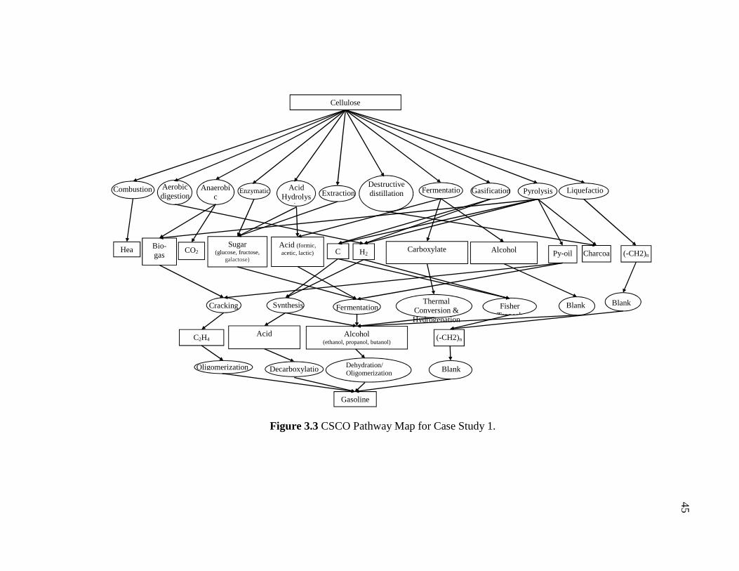
on various technologies that are found in open literature, the CSCO pathway map is
developed as shown in Figure 3.3. The ‘Blank’ operators (as shown in Figure 3.3) are
employed in the CSCO representation to allow a chemical species to go unchanged
through a layer.
The synthesis problem is formulated as a linear program and solved using the
optimization software LINGO (version 10). Once a solution is obtained, an integer cut is
added to exclude the solution and to generate another one. The procedure is continued
until the value of the objective function drops below the maximum yield obtained in the
first solution.

44
Table 3.1 Key Reactions for Case Study 1
From Pathway To Reaction
C6H10O5
Hydrolysis Anaerobic digestion
C6H12O6 CH4
C6H10O5 +H2O → C6H12O6 C6H10O5 +H2O → 3CO2 + 3CH4
CO2 Gasification CO C6H10O5 + O2 → 6CO +4H2+H2O
H2 Fermentation Carboxylate 1.5CaCO3 + C6H10O5 +H2O →
1.5(CH3COO)2Ca +1.5CO2+0.5H2O CO2
C6H12O6
Anaerobic digestion
CH4
C6H12O6 → 3CO2 + 3CH4
CO2 Gasification CO C6H12O6 + O2 → 6CO +4H2+2H2O
H2 Fermentation Carboxylate 1.5CaCO3 + C6H12O6 →
1.5(CH3COO)2Ca +1.5CO2+1.5H2O CO2 CH4 Cracking C2H4 CH4 + 0.5O2→ 0.5 C2H4 + H2O CO2 Water gas shift CO CO2 + H2 → H2O + CO
Carboxylate Thermal conversion
Alcohol CH3COOCaCOOCH3→CaCO3+CH3
COCH3 CH3COCH3 + H2→ CH3CHOHCH3
CO Synthesis Alcohol CO + 2H2→CH3OH C2H4 Oligomerization Gasoline 4C2H4+H2→C8H18
Alcohol Dehydration + oligermerization
Gasoline 8CH3OH+H2→C8H18+8H2O
Alcohol Methanol to olefins process
Olefin CH3OH → CH3OCH3 + H2O CH3OCH3→C2H4 +H2O
CO2 Methanation Methane CO2+4H4 → CH4+2H2O CH4 Steam reforming CO CH4+H2O → CO+3H2
H2 CH4 Dry reforming CO CH4+CO2 → 2CO+2H2
H2
45
45
Figure 3.3 CSCO Pathway Map for Case Study 1.
Blank Blank
Blank
C
Cellulose
Carboxylate Sugar
(glucose, fructose, galactose)
Acid (formic, acetic, lactic)
Bio-gas
(CH ) Py-oil
Gasoline
Charcoal
Hea
Pyrolysis Gasification Destructive distillation
Acid Hydrolys
is
Enzymatic Anaerobic
Aerobic digestion
H2
Combustion
Alcohol (ethanol, propanol, butanol) C2H4
Fermentation
CO2
Cracking
Oligomerization
Fisher Tropsch
Extraction
Acid
Synthesis
Decarboxylation
Fermentation
Thermal Conversion & Hydrogenation
Alcohol
Liquefaction
(-CH2)n
Blank
Blank
Blank
(-CH2)n
Dehydration/ Oligomerization
45

46
Five optimal pathways were generated as shown by Fig. 3.4(a-e). All of them provide a
maximum gasoline yield of 85.5 tonne/day. The first pathway (Fig. 3.4a) uses
gasification to produce syngas which is converted to methanol then dehydrated and
oligomerized to gasoline. The second pathway employs anaerobic digestion to produce
CH4 and CO2. Next, CH4 is dry reformed to syngas with the input of the co-produced
CO2. Syngas is synthesized into methanol and finally converted through dehydration and
oligomerization to gasoline. More water is produced in the process than the required
amount in the digestion. Therefore, the produced water is recycled to replace the fresh
water used in digestion. The third pathways starts with fermentation in the presence of
calcium carbonate to produce calcium acetate, (CH3COO)2Ca which is then treated in
thermal conversion to produce acetone (CH3COCH3) and regenerate the calcium
carbonate (see Figure 3.4c). After that, it is hydrogenated to isopropyl alcohol
(CH3CHOHCH3). Finally, the alcohol is dehydrated and oligomerized to gasoline.
Meanwhile, the CO2 from fermentation is hydrogenated to CO and water and the CO is
synthesized to methanol (CH3OH). Methanol then goes through the same process as
isopropyl alcohol to produce gasoline. In the fourth configuration (Fig. 3.4d), cellulose
is hydrolyzed and fermented to ethanol (C2H5OH) and CO2. Ethanol is oligoermized to
gasoline while CO2 undergoes shift reaction followed by methanol synthesis and
oligomerization. Finally, in the fifth configuration, CO2 produced from anerobic
digestion is converted to methane through a methanation process with the input of
additional hydrogen. Methane from digestion and methanation is converted to syngas
through steam reforming then synthesized to methanol. Finally methanol goes through

47
dehydration and oligomerization to gasoline. Hydrogen produced in the process is
recycled to the methanation step.
It is interesting to note that these five configuration vary widely in their building blocks
and arrangements, yet they provide the same yield. This underscores the value of the
proposed approach in generating promising alternatives without the need to perform
detailed design. Once these potential candidates are generated, effort is focused to these
alternatives and a detailed analysis is properly carried out.
Figure. 3.4(a) Figure 3.4. Five Optimal Pathways for Maximum Yield of Gasoline (Case Study 2)
(all numbers are in tonne/day)

48
Figure. 3.4(b) continued

49
Figure. 3.4(c) continued

50
Figure. 3.4(d) continued

51
Figure. 3.4(e) continued
3.4.2 Case Study 2: Maximum Yield for the Production of Gasoline from Two
Feedstocks with Actual Conversion and Yields
In this case, we increase the level of complexity of the case study by allowing two
biomass feedstocks and by including reported data for conversion and yield. These data
are compiled in Table 3.2. Two types of biomass are considered: 30 tonne/day of
sorghum and 70 tonne/day of municipal solid waste (MSW). Table 3.3 shows the
composition of both feedstocks. Note that the main components in the given feedstocks

52
are cellulose, hemicellulose and lignin. Furthermore, the external supply of hydrogen
was limited to an upper bound of 0.25 tonne/day. The optimization formulation is
developed with the objective of maximizing the gasoline yield. The solution was found
to be a maximum gasoline yield of 26.6 tonne/day and the identified pathway is shown
by Fig. 3.5. It includes fermentation of cellulose and hemicelluloses and pyrolysis of
lignin. The produced alcohol from fermentation is dehydrated and oligomerized to
gasoline. The pyrolysis products are subjected to cracking, oligomerization, and Fischer-
Tropsch synthesis to produce gasoline.

53
Figure 3.5. Pathway for Gasoline Production from MSW and Sorghum (Case Study 2) (all numbers are in tonne/day)

54
54
Table 3.2 Compilation of Conversion and Yield Data for Case Study 2
From Pathway To Conversion
%
Yield (Mass Ratio of Desired Product to Key Feed)
Reference
Cellulosic Municipal
Solid Waste
Anaerobic digestion Bio-gas 80.0 0.210
CO2 80.0 0.473 Rivard (1993) Extraction Sugar
Hydrolysis/Fermentation
Carboxylate 30.2 0.180 Aiello-Mazzarri et
al. (2005)
Acid 90.0 0.800 Schmidt and
Padukone (1997)
Alcohol 90.0 0.511 Krishnan et al.(1999)
Gasification CO 99.0 0.500
H2 99.0 0.071 Filippis et al.
(2004)
Pyrolysis
Py-oil 99.0 0.522 Ojolo and
Bamgboye (2005) Charcoal 99.0 0.242
H2 99.0 0.040 CO 99.0 0.186
Liquefaction Gasoline 95.0 0.260 Minowa et al.
(1995)
Bio-gas Cracking C2H4 92.9 0.580 Fincke et al. (2000)
54

55
55
Table 3.2 Continued
Sugar Fermentation Alcohol 83.0 0.360 Reid and George
(1945)
Acid Fermentation Alcohol 0.900
CO
Synthesis Acid 90.0 0.770 Knifton, (1985)
Alcohol 37.5 0.208
Zhang et al. (2001)
F-T Gasoline 90.0 0.203 Dry (1996)
H2 Synthesis
Acid 90.0 0.108 Knifton (1985) Alcohol 37.5 0.015 Zhang et al. (2001)
F-T Gasoline 90.0 0.014 Dry (1996)
Carboxylate Thermal conversion Ketone 99.5 0.365 Holtzapple, et al.
(1999)
Bio-oil
Cracking (Hydroprocessing) C2H4 99.0 0.250 Bridgwater (2008)
Gasification Syngas
99.0 0.530
C2H4 Oligomerization Gasoline 99.0 1.017 Khanmetov et al
(2006)
Acid Decarboxylation Gasoline 60.0 0.252 Sharma and Olson
(1994)
Alcohol
Dehydration/Oligomerization
Gasoline 99.0 0.619 Costa et al. (1985)
Lignin Pyrolysis
Bio-gas
100.0
0.089
Bio-oil 0.360
CO 0.050 H2 0.020
Gasification H2
100.0 0.075 Jangsawan et al.
(2005) CO 0.018
55

56
56
Table 3.2 Continued
Hemicellulose
Pyrolysis
Bio-gas
100.0
0.089
Bio-oil .360
CO 0.050 H2 0.020
Gasification H2
90.0 0.072
CO 0.170
Fermentation Alcohol 90.0 0.450
Murphy and McCarth (2005)
Acid 80.0 0.760 Jin et al. (2005) Anerobic digestion CH4 80.0 0.180 Enzymic hydrolysis Sugar 90.0 0.830 Adsul et al. (2007)
Table 3.3 Composition of Sorghum and MSW (NREL, 2007)
Wt % Sorghum MSW Cellulose 45 52
Hemicellulose 30 26 Lignin 24 20
56

57
3.4.3 Case Study 3: Minimum Payback Period
Other than targeting the maximum biofuel yield as shown in case studies 1 and 2,
including economic objectives may be desired early enough in the development
activities. In this case study, minimum payback period is selected as the optimization
objective. The intent is to include key economic indicators without getting trapped in an
in-depth economic analysis that will require tremendous time and effort for all the
potential candidates. Tables 3.4 and 3.5 show the cost data for the processing
technologies and the cost/selling price of the targeted species. A feed flowrate of 1,620
tonne/day of cellulose is used. A ten-year linear depreciation scheme is used with no
salvage value. The synthesis task is formulated as a nonlinear programming problem
whose objective is to minimize the payback period and the constraints include the
developed optimization formulation coupled with the data from Tables 3.2, 3.4, and 3.5.
The solution obtained using the optimization software LINGO (version 10) is shown by
Fig. 3.6. As shown, the pathway involves hydrolysis and fermentation of cellulose
followed by dehydration and oligomerization. The produced gasoline is 511 tonne/day.
The solution has an objective function for a minimum payback period of 8.8 years. It is
worth noting that upon further techno-economic analysis, the payback period will be
longer because of the addition of equipment that have not been accounted for in the
program. Nonetheless, the intent of this approach is to quickly provide preliminary
synthesis alternatives that warrant additional analysis. It is also worth noting that once
the cost criterion has been included in this case study, the complexity of the synthesized
solution has significantly decreased compared to the previous two case studies which

58
only focused on yield without cost. This is attributed to the ability of this approach to
exclude pathways or portions of the pathways that will not be cost effective even if they
enhance the yield.
Table 3.4. Cost Data for Case Study 3
Technology AOC per daily tonne
($/yr/daily tonne) α AOF*
($/yr/daily tonne0.7) Combustion 1.00×10⁶ 1.00×10⁶
Aerobic Digestion 1.15×10⁵ 3.62×10⁵ Anaerobic Digestion 1.34×10⁵ 1.97×10⁵
Enzymatic 1.00×10⁶ 1.00×10⁶ Acid Hydrolysis 1.00×10⁶ 1.00×10⁶
Extraction 1.00×10⁶ 1.00×10⁶ Destructive Distillation 1.00×10⁶ 1.00×10⁶ Fermentation (to acid) 8.90×10⁴ 1.19×10⁵
Fermentation (to carboxylate) 2.06×10⁵ 2.14×10⁵ Fermentation (to alcohol) 5.72×10⁴ 1.35×10⁵
Gasification 1.43×10⁵ 2.28×10⁵ Pyrolysis 1.04×10⁵ 1.88×10⁵
Liquefaction 3.33×10⁵ 4.47×10⁵ Methane Cracking 2.43×10⁴ 7.27×10⁵
Acid Synthesis 6.73×10⁴ 8.64×10⁴ Alcohol Synthesis 6.73×10⁴ 8.64×10⁴
Sugar Fermentation 2.86×10⁵ 2.69×10⁵ Thermal Conversion 1.17×10⁴ 1.92×10⁵
Fisher Tropsch 3.01×10⁵ 4.70×10⁵ Pyoil Gasification 8.91×10⁴ 4.46×10⁵
Pyoil Cracking 5.98×10⁴ 4.55×10⁵ Oligomerization 2.16×10⁴ 3.89×10⁵ Decarboxylation 2.85×10⁵ 1.65×10⁵
Dehydration 3.57×10⁴ 4.37×10⁴ *The AFC is modeled using the following formula: AFC = α*Flowrate0.7

59
59
Table 3.5. Costs and Selling Prices for the Species of Case Study 3
Species Price Cellulose 60 $/tonne Gasoline 3.1$/gal Biogas 6.86$/1000SCF Sugar $765/tonne Acid $1,496/tonne H2 4,000$/tonne
Carboxylate $1,100/tonne Alcohol 3.2$/gal Pyoil 2$/gal
Charcoal 77$/tonne C2H4 $1,386/tonne H2O $1.5/1000gal
CaCO3 65$/tonne O2 $210/tonne
59

60
60
Figure 3.6 Solution to the Problem of Minimum Payback Period (Case Study 3) (all numbers are in tonne/day)
60

61
3.5 Conclusions
In this paper, a shortcut method has been introduced for the conceptual design and
preliminary synthesis of alternative pathways of the process industries with focus on the
applications for biorefineries. The chemical species/conversion operator structural
representation has been introduced. It tracks chemical species, connects various streams
with processing technologies, and embeds potential configurations of interest. An
optimization formulation has been developed to maximize the yield or the economic
potential subject to constraints that include process models, distribution of streams and
species over the conversion technologies, interconnection of the candidate technologies,
and techno-economic data. Three case studies have been solved to demonstrate the
effectiveness and applicability of the developed approach. The case studies covered the
scenarios of maximum theoretical yield, accounting for actual process yield, including
more than one feedstock, and incorporating an economic objective (payback period),
The solutions of the case study illustrate the ability of the proposed approach to generate
a wide variety of pathways that achieve the same target but vary significantly in their
building blocks and interconnections. The solution of the case studies also demonstrate
that by including an economic objective function that the complexity of the devised
pathways is greatly reduced.

62
4. AN INTEGRATED APPROACH FOR THE BIOREFINERY PATHWAY
OPTIMIZATION INCLUDING SIMULTANEOUSLY CONVERSION,
RECYCLE AND SEPARATION PROCESSES
4.1 Abstract
Biorefinery is an industrial facility that produces a lot of products from biomass, and
nowadays it has gained a lot of attention because the increasing depletion of fossil fuels
and the environmental problems caused by the use of fossil fuels. In this regard, biomass
can be considered as a sustainable resource and it provides significant environmental
benefits because the reduction of the greenhouse gas emissions. While there are
tremendous technologies and pathways concerning the selection for a biorefinery, this
work presents a systematic approach to determine the optimum pathway of technologies
to convert biomass into biofuels, combining the necessary steps to recover and recycle
intermediate products during the synthesis. A system of mass treatment network and
technology conversion network is presented to model the problem. Mathematic
formulations are constructed to analyze the optimization network. A case study has been
presented to illustrate the problem for producing gasoline from cellulose, and results
show that the optimal pathway corresponds to alcohol fermentation and oligomerized to
gasoline with a minimum payback period of 11.7 years with 1620 tonne/day of feedstock;
whereas, when the capacity is increased to 120,000 BPD of gasoline production, the
payback period is reduced to 3.4 years.

63
4.2 Introduction and Literature Review
Fossil fuels have been supplying a large share of global energy demand. With the
continuous growth of population and industrial activities, the world's energy
consumption is projected to increase by 49% from 495 quadrillion Btu in 2007 to 739
quadrillion Btu in 2035 (EIA, 2010), while the world crude oil and natural gas reserve
can only last for 50 years (IEA, 2010). The pressure of fossil energy supply for meeting
the increasing demand situation prompts the need to develop alternative energy
resources including hydro, wind, solar, geothermal, marine energy, and biomass.
Biofuels provide a variety of advantages over petroleum-based fuels including: (a) the
biomass feedstock are sustainable and environmentally friendly, (b) biofuels are neutral
in greenhouse gas (GHG) emissions if efficient processes are applied, which can help to
satisfy the Kyoto regulations (Bioenergy, 1998), (c) a wide variety of versatile biomass
can serve as the feedstock and they are easy and cheap to be accessed, and as a result a
large production of fuels or chemicals could be derived, (d) with the increasing price and
depletion of fossil fuels, the biofuels will show promising economical potential and
supplement the energy supply. There have been an increase of public awareness towards
biofuels production, and global government investment to biofuels is projected to rise to
45-65$ billion per year from 2010-2035 (IEA, 2010). In addition, conventional chemical
companies like Shell, Conoco-Phillips, Dupont, Dow and BP between others have been
stepping into the area of developing technologies and processes for producing biofuels
and bio-chemicals (Huber et al., 2006).

64
A biorefinery is a processing facility that can transform biomass to fuels, power, and
value added chemicals by integrating conversion technologies and processes (NREL,
2005; Ng, 2009). A variety of forms of biomass including energy crops, agricultural
wastes, forestry residues and municipal solid wastes can serve as the main resources of
feedstock (Bridgwater, 2003). Biomass components include lignin, cellulose, proteins,
acids, and various other chemicals (Askew, 2005), and the target of a biorefinery is to
obtain the maximum value from the biomass components through optimal processes.
Although biomass has been taken as an input to derive products in extensive applications,
the application of converting it through a complex petroleum like refinery to produce
multiple products is relatively new (Fernando et al., 2006). There are various routes in
biorefineries, among which biological conversion, physical conversion and thermal
conversion are the three main paths for producing bio-energy. Given the intensive capital
cost in a biorefinery, there is a need to explore different levels of integration to enhance
the performance of a biorefinery, which includes increasing the energy efficiency,
maximizing overall value of products derived from feedstock, adding flexibility of
products conversion, and reducing the overall cost.
Much research efforts have been involved in chemical process synthesis (Douglas, 1988).
Rudd (1968) pioneered the process synthesis work in the 1960s,whereas Westerberg
(1980) and Nishida et al. (1981) later defined the process synthesis as an approach to
determine the optimal structure of the process system and the optimal process design to
satisfy the specified performance. Extensive works have been conducted in the synthesis

65
area, including separation sequences, reaction pathways, heat integration, etc. In this
regard, El-Halwagi (1997; 2006) introduced the concept of mass-exchange networks
(MEN) in the area of mass integration and Bagajewicz (2000) presented a review on
various methods for the wastewater treatment and material allocation problem.
There are a few challenges facing the designing and synthesis of multi levels of
integrated biorefineries, these include the complex chemical structures and compositions
of biomass (which increases the difficulty of feedstock analysis and treatment as well as
regional dependent, and lack of established information for the thermodynamic
properties and reaction kinetics (Ng et al., 2010)). This makes many synthesis and
design approaches of conventional chemical processes not compatible for the synthesis
of integrated biorefineries. In this regard, Kokossis et al. (2009) discussed the status and
the challenges for the synthesis and integration of a biorefinery, and they proposed a
systematic approach to identify optimal opportunities for biomass-chemical production
and combining with other technologies. Mansoornejad et al. (2009) presented a
biorefinery framework in marketing decision aspects, through integrating supply chain
design with process design. Bridgwater (2003) presented multiple products and multi-
scale processes in a biorefinery. Sammons et al. (2007) then presented a framework to
evaluate multiple production routes and product portfolios based on profitability
optimization. Later, Sammons et al. (2008) extended the work by including economic
perspective with other process insights to facilitate evaluating an integrated biorefinery
through a mathematic framework to optimize product allocation problems based on

66
environmental and economic measures. Later, Tan et al. (2009) developed a fuzzy linear
programming integrated with an input-output mass-energy balance system to target the
optimum of process units capacities based on product metrics and environmental goals.
At the same time, Elms and El-Halwagi (2009) presented a systematic procedure for
scheduling of biorefineries and biomass resources selection, the optimization was
performed to design and integrate the biorefinery along with the consideration of GHG
emissions reduction. In addition, Ng et al. (2009) proposed a hierarchical approach for
the synthesis and integration of biorefineries to determine promising pathways, where a
sequential screening method was utilized for targeting potential technologies by
analyzing thermodynamic feasibility and gross revenue. Ng et al. (2010) then introduced
an automated optimization method to target the maximum biofuel production and
revenue for an integrated biorefinery, this approach used simple conversion models to
calculate the yield of a biorefinery through a source to sink mass flow structure.
Although the approach by Ng et al. (2010) is convenient in targeting yield estimates, it
does not consider capital investment and only simple technological models could be
applied. Pokoo-Aikins et al. (2010) also presented a method to design and guide the
screening of alternative biorefineries based on safety, process and economic metrics. In
addition, Tay et al. (2011) used graphical techniques of a carbon–hydrogen–oxygen
(CHO) ternary diagram to synthesize and optimize for the performance target of an
integrated biorefinery. Bao et al. (2011) then proposed a structural representation and
optimization approach for synthesis and screening of integrated biorefineries. Research
efforts have also covered optimal biofuel production and optimal energy reduction in

67
designing alternative biorefinery routes (see Gosling, 2005; Alvarado-Morales et al.,
2009). Additionally, detailed techno-economic analyses have been carried out for
biorefineries with thermal cogeneration considerations (Qin et al. 2006; Mohan et al.,
2007; Goyal et al., 2008). Furthermore, design and optimization alternatives have been
conducted for biodiesel production from a variety of feedstock like soybean oil and algal
oil (Myint and El-Halwagi, 2009; Pokoo-Aikins et al., 2010).
On the other hand, mass integration techniques have been effectively used in process
optimization by dealing with the material separation, allocation and conversion of
species and processes. There are mass integration strategies to recycle and reuse process
sources using the pinch analysis method and mathematical programming models (El-
Halwagi, 2006; Pillai and Bandyopadhyay, 2007). Interception systems can be utilized in
the mass synthesis to separate target species from process streams as a strategy for
material recovery and waste minimization. El-Halwagi and Manousiouthakis (1989)
developed an approach for synthesizing mass exchange networks (MENs) to transfer
species between a set of rich streams and a set of lean streams. Later a graphical strategy
for minimizing wastewater was introduced by Wang and Smith (1995). Garrard and
Fraga (1998) and Xue et al. (2000) used generic algorithms techniques to synthesize
MENs. Quesada and Grossmann (1995) presented a mass exchange networks model and
dealt with the bilinear terms. Dhole et al. (1996) presented a graphical supply and
demand composite that relates flow rate versus concentration to locate the water pinch
point. El-Halwagi and Spriggs (1998) presented a source sink system to analyze the

68
recycling problem. Later, Polley and Polley (2000) proposed an approach to optimize the
recycling conditions coupled with material recovery. Multicomponent systems of
material recovering and recycling have also been addressed by Benko et al. (2000), Dunn
et al. (2001a; 2001b), Teles et al. (2008), and Alvarado-Morales et al. (2009) by using
mathematical programming techniques. Manan et al. (2004) developed strategies to
target minimum fresh water using a surplus diagram and design mass recovery using a
non iterative approach in a wastewater treatment problem. Gomes et al. (2007) proposed
a heuristic approach when dealing with synthesizing mass exchange networks, and Ng et
al. (2007a; 2007b) also addressed the problem to get maximum water recycle by
coupling with regeneration system to meet environmental regulations. In addition,
different approaches for mass integration based on different properties have been
recently reported (see Ponce-Ortega et al., 2009; 2010; Napoles-Rivera et al., 2010;
Grooms, et al., 2005).
Therefore, even that the previous improvements identified in the design of integrated
biorefineries, previous methodologies have the following drawbacks: 1) In the previous
methodologies only a few of the existing technology alternatives from experiences could
be suggested, and the real optimum process solutions maybe neglected. 2) They are time
and cost consuming for evaluating each alternative. 3) Since they are derived from
experiences and existing knowledge, the application will be limited. 4) The
simultaneously optimization for the technology and mass recovery selection was not
considered. 5) The optimal interconnecting products and flow rates can not be

69
considered. And therefore, 6) No systematic approach for the optimal cost-effective
design of an integrated biorefinery that considers the optimal selection of conversion,
separation and recycle has been reported.
Therefore, to overcome the drawbacks of the previously reported methodologies, this
paper proposes an approach to synthesize an optimum biorefinery pathway by coupling
conversion techniques with material recycle and reuse to provide a generic biorefinery
synthesis approach. To consider the diverse potential of conversion
technologies/feedstocks and alternative combinations of the pathways in a biorefinery,
there is a strong need to effectively and systematically generate optimal alternatives that
meet specified objective of cost effective, pollution preventive and resources
conservative design (e.g., Azapagic, 2002; Chouinard-Dussault et al., 2011). The target
of the model is to find an optimal alternative of biorefinery pathway that also considers
the process specifications, design and selection of process separation and recover/recycle
besides the conversion technologies. As a result, a systematic approach is developed to
select the optimal biorefinery pathway. The optimal allocation of conversion
technologies, recycle design and interconnecting flow rates are determined for the
selected feedstock and products.
4.3 Problem Statement
The problem addressed in this paper is defined as follows.

70
Given a process with:
1. A set of biomass feedstock: FEEDSTOCK = r| r = 1, 2, …, NFEEDSTOCK. Each
feedstock has a given flow rate Hr and a given composition CFRESHc,r.
2. A set of desired primary products: PRODUCTS = pr| pr = 1, 2, …, NPRODUCT. Each
product requires a flow rate Wpr and composition CPRODc,pr that satisfy the following
constraint:
, ≤ , ≤ , , ∈ , ∈
≥ , ∈
where , and , are given lower and upper bounds on acceptable
component composition c for products pr, and is given lower bounds on
acceptable flow rate for products pr.
3. A set of interception units: INTERCEPTORS = u| u = 1, 2,…, NUNITS that can be
used to treat each component composition c.
4. Available for service is a set of processing (conversion) technologies: TECH = g| g =
1, 2,…, NTECH with known characteristics of performance (e.g., yield, unit cost,
composition).
The objective is to synthesize a biorefinery and develop an optimization method to
determine the following:
1. Minimum cost of the biorefinery pathway including the cost of conversion
technologies, separation and recycling that satisfy the process requirements.
2. Optimum selection of conversion technologies and feedstock.

71
3. Optimum pathway of conversion technologies and process flow rate allocation.
4. Optimum selection and allocation of interception units.
The conceptual design procedure proposed in this paper is intended to screen the
numerous alternatives, to produce an optimal technology pathway of the major process
components of the biorefinery, and to perform a detailed techno-economic analysis.
4.4 Approach and Mathematical Formulation
The methodology presented in this paper consists in a systematic approach and
mathematical formulations (as it shown in Figure 4.1). First the systematic approach is
presented and then the mathematical programming formulation is shown.

72
Figure 4.1 Proposed Solution Approach.
First, based on the available biomass and desired fuel products, targetting is performed
before the optimization steps to evaluate the best feasible solution. Then, the information
of all the available technologies and intermediate products is collected for a pathway tree

73
construction. After that, the mathematic model is formulated to select the optimal
pathway based on certain objectives with necessary constraints. If the objective is met,
then the solution will be output as the optimal pathway with the intermediate products
and technologies selected. If the objective is not met, the pathway tree is revised and the
constraints are changed for the mathematical optimization again until the objective is
met.
4.4.1 Systematic Approach
The problem is formulated as a network representation, and this network is categorized
into conversion (technologies) operator block and material separation block. The
analysis is started with the following steps:
1. List the available conversion technologies along with their performance characteristics
(e.g., yield, unit cost) based on literature survey, simulation, reaction pathways synthesis,
etc. The constraints (inlet components concentration, operation conditions, properties,
etc) for each technology are listed as well.
2. Based on the characteristics of the biomass feedstock, the desired products, and the
conversion technologies, develop a list of the candidate chemical species that may be
involved in the biorefinery. Let c and NSPECIES be the index and the total number of
the chemical species, respectively. Also, use a list of candidate compositions that are
used to track the process streams and break the biomass feedstock into key chemical
species (quantified based on chemical analysis).

74
3. Based on the available chemical species and the performance characteristics of
products from the available technologies, list the possible units that can be used to treat
each component. Simulation or preliminary calculations of separation scheme with some
heuristic rule are carried out first. Let NUNIT be the total number of available units. The
performance and inlet conditions of the units are also included to select the optimum
treatment units. Environmental requirements are considered wherever necessary.
4. After the previous steps are performed, the two blocks of conversion operator and
material separation system are interconnected with the process streams mixing and
splitting. Then, a network of the synthesized pathway is constructed and the
mathematical model is finally formulated to optimize the system.
The outline for the mathematical model is given in the next section.
4.4.2 Outline for the Mathematical Model
The conversion operator-interception-conversion operator representation proposed in
this paper is shown in Figure 4.2. The diagram is comprised of alternating layers of
conversion technologies followed by the interception network. There are NP layers of
conversion operators and each layer is designated by the index i. The conversion
operators in the first layer (i=1 ) accept flow rates from feedstock. There are NFEEDSTOCK
of feedstock and each feedstock is designated by the index r. Each feedstock is allowed
to split to different process convertors. The convertors in the last layer (i=NP) are used
to store process streams unchanged into product acceptors. There are NPRODUCT products

75
and each product is designated by the index pr. Streams fed into conversion operator gNP
go unchanged into product acceptor pr with the relation of gNP = pr. Each process
convertor gi can accept multiple streams from the mass treatment system, and the
streams produced from each conversion operator gNP is segregated into unknown flow
rates and are allocated to the mass treatment system to be treated and recycled. Within
each conversion operator, the streams with specific component characteristics can be
converted to streams with new or intermediate species, and those intermediate species
can be treated and further converted through other technologies to finally produce the
desired products. Within the interception network, the composition of each stream is
altered if an interception device is used. After the separation and purification steps are
carried out, the streams leaving the interception network are allowed to mix and fed to
process convertors in the next layer or recycled to previous layers.

76
gi=1 gi=2 NGigi…...
g1=1 g1=2 NG1g1…...
r=1 r=2 r r=N…...
gNP=
1
gNP=
2NGNPgNP
…...
pr=1 pr=2 pr NPR…...
Feedstock
Conversion-
operator layer i=1
Conversion-
operator layer i
Conversion-
operator layer
i=NP
Product
MASS
TREATMENT
SYSTEM
Figure 4.2 Conversion Operator-Interception-Conversion Operator Representation for Biorefinery Pathway Synthesis.

77
The more detailed structure of the mass and property treatment system is shown in
Figure 4.3. The mathematical model is based on the configuration shown in Figure 4.3,
and it includes mass and material balances at mixing points of each process streams,
mass balances at splitting points, and process and performance constraints. It is a source-
sink network integrated with a technology convertor system. All the process streams
coming from the conversion operators with flow rate , represent the process sources
for the interception network, and all the process streams entering the operators with flow
rate , represent the sinks for the interception network. An optimum allocation of
operation convertors gi is determined and an optimum flow rate connecting these
convertors is determined. Each source is segregated into fractions and allocated to the
interception network. Streams leaving the separation network are mixed before entering
each sink. The splitting fractions and mixing ratios are optimized. In the mass treatment
network, there are NUNITS treatment units with index u to refer to each unit, and NKi
discretized interceptors to treat each stream. Each unit has a certain interception extent,
efficiency and cost performance. The optimum interception for the streams and selection
of treatment units are determined.

78
Figure 4.3. Structural Representation of the Mass Treatment Network Integration with Conversion Operator.

79
A blank unit is put in the interception system to allow a stream that need pass through
the system unchanged. An additional sink is placed to represent the waste material. Also,
some external fresh resources can be purchased to supplement the use of existing process
streams.
4.4.3 Mathematical Formulation
The foregoing concepts can be conducted in an optimization formulation that involves
the following model.
The performance model (shown in Figure 4.4) for conversion operator gi in layer i
(referred to as ,,) relates the flow rates of the different streams entering and leaving
the conversion operator:
(, , ,,) = ,,, ,,,,,,,, ∀ ∈ , ∈ , ∈
(4.1)
where , and , are the flow rates of process streams leaving and entering the
conversion operator gi in layer i. And ,, and ,, are the composition for
component c of process streams leaving and entering the conversion operator gi. The
design and operating variables of gi are denoted by , and igO , respectively.

80
Figure 4.4 Mixing and Splitting Representation Around the Conversion Operator.
The mass balance around the conversion operator indicates that the total flow rates
coming out of the operator gi in layer i should not exceed the flow rates fed into the
operator gi:
, ≤ , , ∀ ∈ , ∈ (4.2)
Splitting of fresh sources: Fresh sources can be split and sent to any sink but not to the
waste to satisfy the treatment capabilities. Feedstock can be among those fresh sources.
= ∑ ∑ ℎ,,∈∈(,) !
, ∀ ∈ , ⊂
(4.3)
Splitting of process sources: Process sources are split and sent to each treatment unit:

81
, = ∑ ∈, , ∀ ∈ , ∈ (4.4)
Mass balance in the splitting point at the exit of the interceptors: The flow rate of
streams leaving the interceptor is equal to the summation of streams sent to the available
sinks and the waste.
∑ ∑ ,,∈∈ = , ∀ ∈ (4.5)
Mixing of streams entering the sinks: The flow rate entering each sink is equal to the
summation of the streams from the interceptors plus the fresh sources.
, = ∑ ,,∈ + ∑ ℎ,,∈" , ∀ ∈ , ∈ (4.6)
The component balance around the mixing point before the sinks is given by the
following equation:
,,, = ∑ ,,∈ , + ∑ ℎ,,∈" ,#! ,∀ ∈ , ∈
, ∈ (4.7)
Mixing of waste: Streams leaving the network are allowed to mix into the waste block.
!"# = ∑ ,(,)$ !∈ (4.8)
The performance function for the uth interceptor is given by the following relationship:
, = $,, ,, ∀ ∈ , ∈ (4.9)

82
Previous relationships state that the composition of each component c in the output
stream from interceptor u is the function of the design and operating factors
(these could be the temperature, pressure, solvent selection, catalyst, etc.) and the
composition of the stream fed to the unit. Notice that each unit has specific constraints.
Constraints: A set of constraints for the process convertors is needed for the process
limits and environmental regulations. These include the constraints for the quality of the
products, given in terms of upper (≤ ,, ) and lower bounds (,,) for
the composition of the product.
,, ≤ ,, ≤ ,, ,∀ ∈ , ∈ , ∈
(4.10)
The environmental constraints for the waste generated are stated in terms of upper
(, !% ) and lower (, !%) bounds for the composition as follows:
, !% ≤ , ! ! ≤ , !% ,∀ ∈ (4.11)
The feedstocks are fed to the technologies in the first layer:
∑ ℎ,&,∈ = ,∀ ∈ , ⊂ (4.12)
Notice that the index r refers to the feedstock, which is among the total fresh sources.
No streams can enter to the technologies in the first layer other than the feedstock:
,&, = 0, ∀ ∈ , ∈ (4.13)

83
Bounds for the product flow rate: The flow rates of products require lower bounds. The
streams entering to the convertors in the last layer NP are equal to the streams of the
desired products; therefore, the flow rates of the streams entering to the convertors in the
last layer require the following lower bounds:
,
≥
,∀ ∈ (4.14)
A particularly useful special case is when the concentration of each component c leaving
the conversion operator gi is calculated through a given yield (%..)times the
concentration of a limiting component (lim
igc ):
,, = %.. × ,,
,∀ ∈ , ∈ , ∈ (4.15)
Note that the concentration of all the components c should be less than or equal to 1.
∑ ,,∈ ≤ 1, ∀ ∈ , ∈ , ∈ (4.16)
The flow rates of the different chemical species entering to the conversion operator gi are
related to the flow rate of the limiting component via a stoichiometric or another form of
required ratio (denoted by &..). Hence, the following relationship is included in the
model:
,, = &.. × ,,
,∀ ∈ , ∈ , ∈ (4.17)

84
The total annualized cost of the conversion operator gi in layer i is given by a cost factor
(',) times the flowrate of the limiting component entering to the conversion operator:
, = , × ',,∀ ∈ , ∈ (4.18)
The total annualized cost for the interceptor u is given by a cost factor (() times the
flowrate of the stream entering to the interceptor:
= × (,∀ ∈ (4.19)
The pollutant removal for the uth interceptor is given by the following relationship:
, = 1 − × ,
,∀ ∈ ∈ (4.20)
Where ) is the efficiency for unit u to remove the pollutants.
Objective function: The objective function consists in to maximize the net annual profit
(), constituted by the annual sales of products minus the cost of fresh sources,
minus the cost of the pathway technologies used to convert the feedstock to products
(, ), minus the cost of selected interceptors to treat the process streams
().
max = * ,' × ''
− * ∈"
×
− * * ,∈∈
− * ∈
(4.21)

85
Where, ' and are the unit cost for the products and fresh sources
respectively.
The cost of technologies gi is related to the flow rates entering to the convertor and the
type of convertor selected (Ω,). In addition the cost for the technology selected depends
on the design and operating parameters as follows:
, = Ω,, ,,,,,∀ ∈ , ∈ (4.22)
The total cost for technology g in the ith layer is a function of the design and operating
factors and the flow rate fed into the conversion technology g.
Previous relationships constitute a mathematical programming problem that could be
linear and the problem can be solved globally to determine the biorefinery configuration
including the flows interconnecting the various conversion operators and the optimum
interceptors for treatment of required properties. If the relationships are not linear and
non convex, appropriate non linear programming solutions methods must be use to get
the optimal solution.
4.4.4 Remarks for the Methodology Presented
• The proposed methodology considers simultaneously the optimal selection of
conversion technology, separation and recycle for the synthesis of a biorefinery.

86
• The problem could be formulated as a linear programming problem to guarantee the
optimal solution.
• To reduce the cost burden and process complexity, layers of technologies are limited
to 3.
• Fresh streams include feedstock and necessary external species for the technologies
conversion.
• The input stream output from the conversion operator are taken as input stream for
the mass treatment system, and output stream from the mass treatment system are
taken as input for the conversion operator.
4.5 Case Study
The following case study is used to illustrate application of the proposed approach.
There are 3 layers of conversion technologies, and the feedstock is selected as cellulose.
There are 11 technologies to convert biomass into intermediates (see Table 4.1), and
these 11 intermediates can be further processed to other products until producing bio-
gasoline. After each technology, there are the separation units to recover the necessary
products. The separation cost of each unit for different sources is listed in Table 4.1
(information taken from Perry and Green, 1984; Peters, 1991; Sinnott, 2005; Vatavuk,
1990; Watson, 1999). The unit cost for treating the waste is 0.22$/tonne. The data for
yield, conversion, unit costs for each considered technology were taken from Bao et al.
(2011). The pathway tree is constructed and the problem is solved using the
mathematical model shown in the previous section using the Lingo software to get the

87
global optimum solution, where a variety of selections could be chosen. The solution for
the minimum payback period of the optimal pathway with separation unit is shown in
Figure 4.5, which corresponds to the pathway with cellulose fermented to alcohol and
alcohol dehydrated to gasoline with a payback period of 11.7 year with 1620 tonne/day
of feedstock. In addition, the second best solution is shown in Figure 4.6 and it
corresponds to the pathway with cellulose fermented to carboxylate and carboxylate
thermal converted to ketone and hydrogenated and oligomerized to gasoline with a
payback period of 12 years. It is noteworthy to mention that when the capacity is
increased to 120,000 BPD of gasoline production, the payback period for both previous
solutions are 3.4 years and 4.2 years, respectively. This information is very important,
because the proposed approach allows to indentify the production required for a desired
payback period.

88
Table 4.1. Separation Cost for Various Streams from Different Sources.
Source stream Technology Separation Removal efficiency (%)
Cost ($/kg recovered)
Cellulose Anaerobic digestion Methane separation
10 0.01
60 0.02 95 0.03
Fermentation to alcohol
Filter and Liquid separation
95 0.03
Gasification Syngas separation 10 0.003 50 0.006 70 0.012 95 0.023
Fermentation to carboxylate
Filter & Liquid separation
95 0.03
Fermentation to acid Filter& Liquid separation
95 0.03
Pyrolysis Syngas separation 10 0.004 50 0.008 70 0.015 95 0.025
Liquefaction Filter 95 0.02
Lignin
Pyrolysis
Syngas separation 10 0.008 50 0.015 70 0.02 95 0.03
Gasification
Syngas separation 10 0.004 50 0.008 70 0.015 95 0.025
Hemicellulose
Pyrolysis
Syngas separation 10 0.008 50 0.015 70 0.02 95 0.03
Gasification
Syngas separation 10 0.005 50 0.01 70 0.016 95 0.026
Fermentation to alcohol
Filter and Liquid separation
95 0.02
Fermentation to acid
Filter and Liquid separation
95 0.015
Anaerobic digestion
Methane separation
10 0.01 60 0.02 95 0.03
Enzymatic hydrolysis
Filter and Liquid separation
95 0.01

89
Table 4.1. Continued
CH4 Cracking Ethylene
separation 95 0.02
Sugar Fermentation to
alcohol Liquid separation 95 0.02
CO Synthesis to acid Liquid separation 95 0.01
Synthesis to alcohol Liquid separation 95 0.012
FT Liquid separation 95 0.01
Pyroil Cracking Ethylene
separation 95 0.02
gasification
Syngas separation 10 0.002 50 0.005 70 0.01 95 0.02
Acid Decarboxylation Liquid separation 95 0.01
Alcohol Dehydration Liquid separation 95 0.01
In Figure 4.5 (optimal solution), the pathway starts with hydrolysis of cellulose to
alcohol. After separation of alcohol from CO2 and other byproducts, alcohol and external
H2 input is converted by dehydration and oligomerization into gasoline. Gasoline is
separated from water byproducts to get the final products of 511 tonne/day. On the other
hand, in Figure 4.6 for the second best solution, the pathway starts with the fermentation
of cellulose into carboxylates. After separating carboxylates from water and lignin
residues, the carboxylates are further converted by thermal conversion into ketones.
After separation and recovery, CaCO3 is recovered and recycled back to supply the fresh
feed, and the recovered ketones are hydrogenated with external H2 and through
oligomerization and hydrogenation converted into gasoline products. Separation steps
are applied to remove the excess water to get the final product (i.e., gasoline) with flow
rate of 234 tonne/day.

90
Figure 4.5 Optimal Pathway for the Case Study (Alcohol Fermentation).

91
Figure 4.6 Second Best Solution Identified for the Case Study (Carboxylate Thermal Conversion).

92
4.6 Conclusions
This work presents a new methodology to effectively optimize a biorefinery technology
pathway integrated with species separation and recycle networks. The proposed
methodology allows to determine the optimal allocation of the conversion technologies
and the recycle. In addition, the proposed methodology is able to identify the cost
effective process of conversion technologies combinations and the optimal
interconnecting flow rates for the selected feedstock and desired products.
A case study has been conducted to illustrate the proposed approach, and results show
that the optimal pathway for the gasoline production from cellulosic materials
corresponds to the alcohol fermentation through oligomerization with a minimum
payback period of 11.7 years; whereas the pathway of cellulose fermented to carboxylate
and carboxylate thermal converted to ketone and hydrogenated and oligomerized to
gasoline has a payback period of 12 years for 1620 tonne/day of cellulose feedstock.
When the capacity is increased to 120,000 BPD of gasoline production, the payback
period for each case is 3.4 years and 4.2 years, respectively. These results allow to
identify optimal pathways and to analyze different scenarios for the implementation of a
biorefinery. Finally, the proposed methodology is applicable to different cases, and the
systematic approach allows to solve easily a problem that originally is complicated.

93
5. A SYSTEMATIC TECHNO-ECONOMICAL ANALYSIS FOR THE
SUPERCRITICAL SOLVENT FISCHER TROPSCH SYNTHESIS
5.1 Abstract
Supercritical solvents offer significant economic benefits in the synthesis of biofuels
using the Fischer-Tropsch synthesis technology. The current study is focused on the
methods to efficiently recycle the supercritical solvent from the Fischer-Tropsch
synthesis products (referred to as light hydrocarbons, syncrude and water) while taking
advantage of the high pressure operation in the reactor bed of the supercritical solvent
Fischer-Tropsch synthesis. In addition, the study is aimed at ensuring the recovery of
middle distillates product as well (jet fuel and fuel fractions of the syncrude). Several
parameters were investigated and optimized in this process, including the separation
sequence and the heat duty (energy consumption) of the separation units. Results show
that from the proposed separation configuration, the solvent is recovered 99% from the
FT products, while not affecting the heavier components recovered and light gas
recovery, and 99% of wastewater is recycled. The case that uses super critical fluids in
the Fischer-Tropsch process is competitive with the traditional FT case with a similar
ROI of 0.26 year. The proposed process has comparable major parts cost with typical
gas to liquid process and the capital investment per BPD is within the range of existing
gas to liquid plant. In addition, several scenarios have been analyzed to show potential
configurations comparable with the optimal one for the FT process.

94
5.2 Introduction
Fischer-Tropsch (FT) reaction has been studied and investigated for nearly a century,
and it is basically described as converting synthesis gas into value added chemicals and
fuel products. The rapid increasing interest on this technology comes from the notice
that natural gas (GTL: gas to liquid), coals (CTL: coal to liquid), biomass (BTL: biomass
to liquid) and other types of wide available resources can be utilized to produce high
value fuels (Alden, 1946; Schulz, 1999). The products are of large range from methane
to wax, and types from branched compounds to oxygenates. The diesel produced from
FT has quality of high cetane number and no sulfur, less CO, NOx and particles resulting
in an environmental friendly fuel.
The application of supercritical fluids in the Fischer-Tropsch synthesis (SCF-FTS) is
aimed mainly at low temperature (LTFT) reactor (Eilers et al., 1990; Fox and Tam,
1995). LTFT bases the main target to produce long chains wax and diesel, by utilizing
the catalyst type of either precipitated iron or supported cobalt (Anderson,1956), and
reactor choice between fixed bed or slurry reactor (Caldwell and van Vuuren, 1986). In
high temperature Fischer-Tropsch (HTFT) there is no liquid phase outside the catalyst
particles, which is the major difference from the LTFT (Steynberg and Dry, 2004).
HTFT usually utilizes a fused iron catalyst with fluidized bed reactor to produce
syncrude including light olefins and gasoline (Steynberg et al., 1999).

95
The first type of LTFT reactor is the fixed bed reactor. It is worth noting that the FT
reaction is highly exothermic; therefore, a large number of tubes is required to remove
the heat released from the reactor and this brings in the problem of poor economies for
scaling up. In addition, the non uniformity in the temperature profile resulting from the
tubes needs increases the catalyst loading rate. This design also results in high pressure
drop, and thus high compression costs (El-Bashir et al., 2010). To avoid previous
problems, Sasol developed a slurry bed FT reactor that uses a fluid media (i.e., wax
produced from the reaction) to operate the reactor as a continuous stirred tank reactor
(CSTR) to keep a uniform temperature profile throughout the reactor (Jager and
Espinoza, 1995). Therefore, the catalyst activity is kept high under uniform temperature
and a good products selectivity is achieved. In addition, this design brings low
compression cost. However, the difficulty in separation of the solid catalyst from the
liquid products remains as a problem in this type of reactors (El-Bashir et al., 2010).
Therefore, there is urgent desire to combine the simplicity of fixed bed reactor and take
advantage of slurry reactor to improve the FT reaction performance. SCF-FTS provides
the platform for this concern, as supercritical fluid has the advantage of gas like
diffusivity and liquid like solubility. Operating FTS under supercritical fluid (SCF)
conditions improves the catalyst selectivity and activity. In addition, SCF can provide
benefits as provide high solubility in extracting heavy hydrocarbons from the catalyst
and excellent heat transfer performance for the reactor. Furthermore, the superior
diffusivity feature eliminates the molecule transport limitations and enhances high α-

96
olefin selectivity for products (Jacobs et al., 2003; Yokota et al., 1990; Bochniak and
Subramaniam, 1998; Durham et al., 2008).
One of the first works in SCF-FTS was undertaken by Yokota and Fujimoto (1989),
where they evaluated the products, solvent and reaction performances of the FTS
reaction under supercritical phase, under gas and under liquid phases, and compared the
results among these conditions in fixed bed reactor and suggested encouraging future for
SCF-FT. Yokota et al. (1990) and Fan et al. (1992) also conducted research on the
catalyst characteristics, hydrocarbon selectivity and reaction performance under the
effect of solvent in SCF-FT analysis. Bochniak and Subramaniam (1998) took a study
for SCF-FTS process and investigated different pressure conditions for the reaction
performance and compared their influence on the catalyst. Huang and Roberts (2003)
carried out a series of experiments using different catalysts and identified several
benefits for the SCF-FTS reaction with cobalt catalyst. El-Bashir and Roberts (2005)
conducted SCF-FTS reaction research using cobalt catalyst and found out that the
standard Anderson-Shutlz-Flory (ASF) model does not apply in near-critical and
supercritical conditions. Recently, El-Bashir et al. (2009) reported a solvent recovery
model under SCF conditions and proposed a design for the optimization of SCF
separation processes as part of FT reactor design.
Previous researches provide a good perspective for the FT reactor. However, previous
researches did not consider the large cost and energy associated with using supercritical

97
fluid operation, and did not notice the design of separation solvent from liquid products
from process optimization view. Proper selection of separation conditions plays a vital
role in obtaining desirable performance. Therefore, this paper proposes a new design for
the separation process of supercritical solvent from reaction mixture optimizing the
pressure drop and the temperature to separate the light hydrocarbons fractions as well as
the permanent gases (syngas and CO2) from reaction mixture coupled with Radfrac
distillation to improve the separation efficiency. Success in utilizing pressure drop in the
separation processes for supercritical phase FTS could represent a major advantage for
this process over conventional FTS technologies since it has always been challenged by
the high price needed for the compression process in addition to other costs associated
for high pressure equipments. Therefore, this paper is focused on the design of
separation sequences of the supercritical solvent as well as the rest of the process by
utilizing the energy from the potential of manipulating the high pressure and temperature
profile from the FTS reaction, in order to evaluate the potential of SCF-FT to beat
traditional FT design.
5.3 Problem Statement
The focus of this paper is to investigate the cost and energy analysis of the gas to liquid
(GTL) process with supercritical fluids in FTS, and to evaluate the potential to compete
with the non supercritical FT process. The main process differences between the two
types are the products distribution range, the reactor operation, and the SCF
incorporation and recovery. Therefore, the paper focus on the step to recover

98
supercritical solvent to reduce cost and obtain sustainable operations. To recover the
solvent from the SCF-FT products, there are several elements to consider: products
purity, products yield, solvent purity, solvent recoverability, energy cost, and operation
feasibility.
The objective of this work is to minimize the process cost and energy consumption,
while maintaining no less than 95% of solvent recoverability, with consideration for
constraints of hydrocarbon products recoverability and purity, and ease of operation.
Also, the work is aimed at taking advantage of the high pressure operation in the reactor
and comparing the process cost of the SCF-FT and non SCF-FT.
5.4 Proposed Approach
This paper proposed a systematic approach to deal with the addressed problem. The
approach is conducted in two main steps and the details are shown in Figure 5.1.

99
Process
Alternatives
Process
Simulation
Oil-Solvent
input
Separation design
constraints
Operating
variables
Process
IntegrationObjective?
Experimental
Validation &
Cost analysis
yes
no
Design, Operating
output
Change Operating
variables or oil
solvent input
Figure 5.1. Proposed Approach for the SCF-FT Solvent Recovery Technology.
In the first step, the approach starts with formulating design and operating variables prior
to selection of the optimum separation design. Firstly, a preliminary flowsheet is
established, and separation design specifications are analyzed and searched from the
literature with the basis of the input oil-solvent mixture characteristics. They are then

100
synthesized and sent to simulation software to generate the mass and heat balance for
later steps. Alternative scenarios are generated based on the performance condition of
the process (arrangement of the sequence of separation units, selection of the units and
the operating conditions of the units). Then, energy integration is performed to target the
minimum energy cost for each scenario and an economic analysis is conducted for each
synthesized process. A certain objective metric is generated based on either cost
optimization, material conservation or environmental efficiency, and it is used to
compare the process performance of each scenario. Certain constraints are also given
including recoverability, composition requirement, etc to assist the optimization step.
After that, if the objective is met, the data are used for experimental validation and
economic evaluation; otherwise, the input data is adjusted and refined, and the previous
steps are went through again until qualified optimum design alternatives are generated.
The second step is to compare the potential of the generated process with the process
without SCF utilization. The comparison is based on certain metric of cost, energy
efficiency or products yield. The first step of SCF separation process design could be
embed in this step.
5.5 Generic Mathematic Formulation for the Separation Design Selection
This section presents the generic mathematic formulation for the selection of the optimal
separation design. Figure 5.2 shows the schematic representation of the addressed
problem. Given a series of scenarios k of different separation design processes, it is

101
desired to select the optimum case k that has the maximum return of investment (ROI).
In each case k there is a sequence of units j to choose from, and there are feedstocks and
external input streams RawFlow(i), and output and products streams ProdFlow(i). Some
output streams including solvents and water could be recycled back as input streams.
Figure 5.2. Mathematic Formulation for the Optimum Separation Designing.
The objective is to maximize the return of investment (ROI):
ObjectiveFunction = MAX (#"+,$+-#!".#+") (5.1)
And the return of investment is the annual net profit divided by the total capital
investment (TCI):
= (#
((()!) (5.2)
The total capital investment is the summation of the working capital investment and the
fixed capital investment (FCI):

102
= ,/+ " 0+-#!".#+" + (1#2 " 0+-#!".#+") (5.3)
The annual net profit is equal to the annual sale minus the annual operating cost, the
annualized fixed cost and the tax:
++ 0+#",$" =3++ 0! 0# − ++ 0,# "+,!" − ++ 04#2$1#2,!"5 × 31 − " 15 +
++ 04#2$1#2,!" (5.4)
The annualized fixed cost is equal to the fixed capital investment minus the salvage
value over the life period:
++ 04#2$1#2,!" = "*!())(
(#' (5.5)
Because only one case k could be selected as the optimal one, the following disjunction
is used to account for the economic aspects.
⋁
/ ∈
677777778 +
++ 0! 0# = **# × ,20,+,
× +,,
=**# × 0,+, × +,,
+ #,!"+
=*1,!"+,,,
× '+,,9:::::::;
Therefore, if the case k is selected, then the binary variable Ek is 1 and the associated
economic parameters for that technology k apply; otherwise, when the technology k is
not selected, Ek is 0 and the associated economic parameters do not apply.

103
The annual sale is the summation of all the products flow rate (,20,+,) multiplied
by the products fraction ( +,,) multiplied by the price of that component c (Pricec).
FCI is the summation of all fixed costs of each unit j multiplied by the size coefficient '.
The annual operating cost (#,!") is the summation of the feedstock cost and other
operating costs (utility, labor, maintenance, etc.). The feedstock cost is the summation of
the entire feedstock flow rate ( 0,+, ) multiplied by the fraction +,, and
multiplied by the price of the component c (Pricec).
To model previous disjunction, the following set of algebraic relationships are used.
Only one case k is selected as optimum:
∑ + = 1+ (5.6)
To find the best possible solution, the above formulation could be solved as follows:
++ 0! 0# ≤ ∑ ∑ # × ,20,+, × +,, + × 1 − + , ∀/
(5.7)
++ 0! 0# ≥ ∑ ∑ # × ,20,+, × +,, − × 1 − + , ∀/
(5.8)
++ 0,# "+,!" ≤ ∑ ∑ # × 0,+, × +,, + #,!"+ +
× 1 − + , ∀/
(5.9)

104
++ 0,# "+,!" ≥ ∑ ∑ # × 0,+, × +,, + #,!"+ −
× 1 − + , ∀/
(5.10)
≤ ∑ 1,!"+,,, × '+,, + × 1 − + , ∀/ (5.11)
≥ ∑ 1,!"+,,, × '+,, − × 1 − + , ∀/ (5.12)
In previous relationships, when the binary variable Ek is equal to one, the relationships
apply properly; on the other hand, when the binary variable Ek is equal to zero, the
relationships are relaxed because of the big M parameter.
In the same way, when the technology is selected, the appropriate relationships for the
mass, component and feasibility constraints apply. This is modeled through the
following disjunction:
⋁
/ ∈
677777778 +
* 0,+, =
*,20,+,
* 0,+, × +,, =
*,20,+, × +,,
,∀ +,, ≥ + +,,∀, ∀
,20,+, ≥ +,20,+,,∀9:::::::;
The overall mass balance of the process for each case k should be equal.
∑ 0,+, ≤ ∑ ,20,+, + × 1 − + , ∀/ (5.13)
∑ 0,+, ≥ ∑ ,20,+, − × 1 − + , ∀/ (5.14)
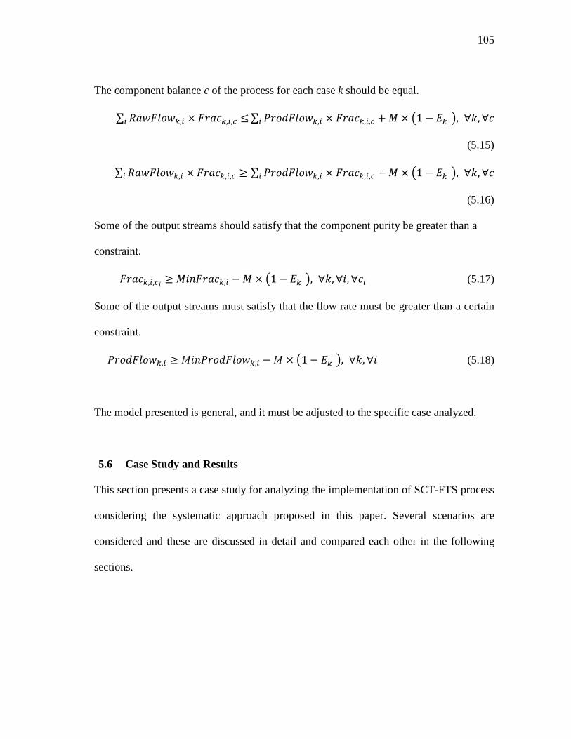
105
The component balance c of the process for each case k should be equal.
∑ 0,+, × +,, ≤ ∑ ,20,+, × +,, + × 1 − + , ∀/, ∀
(5.15)
∑ 0,+, × +,, ≥ ∑ ,20,+, × +,, − × 1 − + , ∀/, ∀
(5.16)
Some of the output streams should satisfy that the component purity be greater than a
constraint.
+,, ≥ + +, − × 1 − + , ∀/, ∀, ∀ (5.17)
Some of the output streams must satisfy that the flow rate must be greater than a certain
constraint.
,20,+, ≥ +,20,+, − × 1 − + , ∀/, ∀ (5.18)
The model presented is general, and it must be adjusted to the specific case analyzed.
5.6 Case Study and Results
This section presents a case study for analyzing the implementation of SCT-FTS process
considering the systematic approach proposed in this paper. Several scenarios are
considered and these are discussed in detail and compared each other in the following
sections.

106
5.6.1 Preliminary Flowsheet Result
Pentane and hexane’s critical properties could qualify as candidate for SCF, since LTFT
typically operates at ranges of 220 to 250 ºC, in addition, they are inert with cobalt and
iron catalyst and show high solubility for other hydrocarbons; hence, in this work
solvent of C5-C7 is selected. As indicated previously, the FTS products are composed of
a variety of hydrocarbon products, gases (CO2 and unreacted CO and H2), and liquids
(water) whereby the hydrocarbons consist of components from light gases of cetane
number approximately 1 up to heavy hydrocarbons with cetane number larger than 30.
In a conventional separation setup, these products are normally separated in three
fraction: (i) permanent gases with light key CO, H2, H2O, C1-C4, (ii) Light hydrocarbons
(e.g. C5-C8), and (iii) Middle and heavy distillates of C9+ components.

107
The FTS products distribution is calculated according to the Anderson-Shutlz-Flory
(ASF) equation (Steynberg and Dry, 2004) following the procedure explained in
Bartholomew and Farrauto (2006) for Shell’s Middle Distillate Synthesis (SMDS)
reactor technology. The chain growth or propagation probability (α-value) is set as 0.96,
and the H2 conversion is set as 73% with syngas feed mole ratio at H2/CO = 2.15. To
reduce the complexity, hydrocarbons with cetane number bigger than 30 are all
represented as C30+ components. The simulated process capacity is assumed to be
120,000 BPD, compared to Sasol setup of approximately 34,000 BPD (Espinoza et al,
1999). The solvent for the SCF- FTS is simulated as C5-C7 and this is co-fed with the
syngas into the FTS reactor at molar ratio of 3:1. The products from the FTS reactor are
obtained from a reaction conditions of 45 bar and 240 °C over cobalt-based catalyst.
Feedstock and products representation at a typical and the aforementioned conditions for
a GTL process are listed in Tables 5.1a and 5.1b.

108
Table 5.1a. Mass Balance for a Typical GTL Process.
Mass Flow (kg/hr)
NG Makeup water
O2 Condense
water Syngas output
Syngas ratio
adjust input
CO2 sequestration
H2 stream production
FT output cobalt 230
H2O - 712,800 - 657,763 657,763 - - - 780,855
METHANE 1,199,785 - - - 7,212 7,212 - - 8,184
NITROGEN 1,764 - 6,360 - 8,123 8,123 - - 8,123
OXYGEN - - 1,445,640 - - - - - -
ETHANE 92,024 - - - 92,024 92,024 - - 93,890
PROPANE 1,039 - - - 1,039 1,039 - - 3,725
CO - - - - 1,547,828 1,547,828 - - 333,171
CO2 20,020 - - - 859,581 - 859,581 - -
H2 - - - - 305,859 237,702 - 68,157 64,180
c4 - - - - - - - - 3,439
c5 - - - - - - - - 4,127
c6 - - - - - - - - 4,754
c7 - - - - - - - - 5,324
c8 - - - - - - - - 5,842
c9 - - - - - - - - 6,309
c10 - - - - - - - - 6,730
c11 - - - - - - - - 7,106
c12 - - - - - - - - 7,442
c13 - - - - - - - - 7,740
c14 - - - - - - - - 8,002
108

109
109
Table 5.1a. Continued
c15 - - - - - - - - 8,231
c16 - - - - - - - - 8,428
c17 - - - - - - - - 8,597
c18 - - - - - - - - 8,738
c19 - - - - - - - - 8,855
c20 - - - - - - - - 8,948
c21 - - - - - - - - 9,020
c22 - - - - - - - - 9,071
c23 - - - - - - - - 9,104
c24 - - - - - - - - 9,120
c25 - - - - - - - - 9,120
c26 - - - - - - - - 9,105
c27 - - - - - - - - 9,077
c28 - - - - - - - - 9,037
c29 - - - - - - - - 8,985
c30+ - - - - - - - - 401,555
- - - - - - - - -
Total 1,314,631 712,800 1,452,000 657,763 3,479,431 1,893,929 859,581 68,157 1,893,936
109

110
110
Table 5.1b. Mass Balance for a GTL Process with Supercritical Conditions.
Mass Flow (kg/hr)
NG Makeup water
O2 condense
water syngas output
syngas ratio
adjust input
CO2 sequestration
H2 stream production
SCFT
H2O - 712,800 - 657,763 657,763 - - - 855,728
METHANE 1,199,785 - - - 7,212 7,212 - - 7,212
NITROGEN 1,764 - 6,360 - 8,123 8,123 - - 8,123
OXYGEN - - 1,445,640 - - - - - -
ETHANE 92,024 - - - 92,024 92,024 - - 92,024
PROPANE 1,039 - - - 1,039 1,039 - - 1,039
CO - - - - 1,547,828 1,547,828 - - 216,696
CO2 20,020 - - - 859,581 - 859,581 - -
H2 - - - - 305,859 237,702 - 68,157 47,541
c4 - - - - - - - - -
c5 - - - - - - - - -
c6 - - - - - - - - 115,194
c7 - - - - - - - - 86,124
c8 - - - - - - - - 71,164
c9 - - - - - - - - 62,330
c10 - - - - - - - - 53,463
c11 - - - - - - - - 43,606
c12 - - - - - - - - 36,480
c13 - - - - - - - - 31,426
c14 - - - - - - - - 25,829
110

111
111
Table 5.1b. Continued
c15 - - - - - - - - 24,893
c16 - - - - - - - - 22,793
c17 - - - - - - - - 18,071
c18 - - - - - - - - 15,395
c19 - - - - - - - - 14,470
c20 - - - - - - - - 11,794
c21 - - - - - - - - 10,368
c22 - - - - - - - - 7,496
c23 - - - - - - - - 5,810
c24 - - - - - - - - 4,950
c25 - - - - - - - - 3,971
c26 - - - - - - - - -
c27 - - - - - - - - -
c28 - - - - - - - - -
c29 - - - - - - - - -
c30+ - - - - - - - - -
- - - - - - - - -
Total 1,314,631 712,800 1,452,000 657,763 3,479,431 1,893,929 859,581 68,157 1,893,988
111

112
The flowsheet and mass balance of the two processes to be compared are shown in
Figures 5.3a (typical) and 5.3b (SCF). The process is composed mainly of autothermal
reactor (ATR) to convert natural gas (NG) into synthesis gas, FT reactor to produce
syncrude from synthesis gas, and the upgrading units. There are units of air separation
(ASU) to generate O2 from air, units to separate CO2, water and other components from
the output gas from ATR, and units to produce H2 from synthesis gas to adjust the
syngas ratio before feed in the FT reactor. In the supercritical solvent FT process, there
are additional separation units to feed fresh solvent to supercritical condition, separate
solvent from liquid products, and separate other products components for further
upgrading. This step is to ensure that: the fresh and recycled solvent are properly mixed,
the temperature and pressure are controlled for syngas and solvent mixture before feed to
the reactor bed, the separation columns are efficient in separating solvent from synthesis
gas, light components, and middle distillates, the pressure drop from the products is
utilized for energy concern.

113
Figure 5.3a. Flowsheet of Typical GTL Process.
113

114
114
Figure 5.3b. Flowsheet of SCF-FT GTL Process.
114

115
The simulation of the solvent/product separation units (Figures 5.4) has been conducted
in Aspen 2006 Plus utilizing the NRTL-RK property method to evaluate the separation
result based on the phase behavior of the product mix. Alkanes are used to model
hydrocarbons from C1 to C30 in this work since they are the major products from the FTS
over the cobalt-based catalyst. The separations units are distillation based, where the
flash column modules play a major role in light hydrocarbons and solvent recovery. The
RadFrac distillation 1 is simulated with 30 stages partial-vapor RadFrac distillate column
with reflux ratio of 2, feed on the first stage and the side draw extracted from the stage
15, the condenser pressure is of 10 bar with a stage pressure drop of 0.1 bar. The
flowsheet of the separation process is described in Figure 5.4.
Figure 5.4. Flowsheet for Supercritical Solvent Separation Process.
The products from FTS (typical outlet products of the FTS reactor bed) (Elbashir et al.,
2009) are represented in stream FT Products where the outlet tailgas recycle streams are

116
represented in the stream Permenant Gas1 and Permenant Gas2, and the outlet solvent
streams are represented by SOLVENT1 and SOLVENT2, the middle distillate and the
heavy hydrocarbons (i.e. C8+) are represented by HEAVY stream while the water outlet
stream is represented by stream water. The separation process starts in the block flash
column1, 2 and 3, where lighter components are initially separated from heavier ones to
reduce large capacity for later separation. The second step in the separation process is
the recovery of middle distillate hydrocarbons in Radfrac Distillation 1. The remaining
lighter fractions from the former steps are sent to Radfrac Distillation 2 and 3. A portion
of Permenant gas could be recovered by a Flash. The Radfrac Distillation 3 will recover
most of the solvent in the bottom of the column. The remaining vapor streams are
separated in the coalesce to obtain the remaining permenant gas, solvent and water. The
separated water is cleaned and reused to purity of 10 ppm to 1000 ppm as indicated in
the patent 7147775. The recovered solvent could be sent back to be mixed with fresh
solvent and feed into the FT reactor. The flow rate of solvent (C5-C7) is averaged among
each component.
The heat duty released or consumed by the flash distillation unit has been accounted for
based on both temperature and pressure factors as shown above. The SCS-FTS is
normally operated at elevated pressure to accommodate the single phase operation for
the reaction mixture as required by this process. Our objective from this analysis is to
take advantage of the high pressure operation and to utilize energy input (for the
compression) in the separation process by utilizing phase split in pressure drop.

117
According to our simulation, as pressure and temperature are dropped, products are
separated and energy could be utilized. Our effort in this study is focused on finding
optimum separation conditions whereby maximum heat release is obtained coupled with
high recoverability of the supercritical solvents and other products. The feed stream of
products from the FT reactor for a solvent- oil syngas ration of 3:1is shown contains by
8% of pergas, 85 % of solvent, 1% of heavier (C8+) and 7% of water.
The condenser/separator system is used for the water/oil product separation after the FT
reactor from patent search of Syntroleum, that condenser/separator is dependent upon
various factors such as overall operating condition, quality and quantity of water
produced by associated Fischer-Tropsch process and quantity and type of contaminants
contained in the natural gas feed stream supplied to autothermal reformer (John, 2004).
One VSEP unit of nano-filtration membranes can be undertaken at pressure of 250 psig
to separate in industrial scale the water from syncrude with the resulting water purity of
16 ppm. Since the water/oil emulsion happen when less than 26% water present in the
system (Hon et al., 2001); therefore, it is desired to separate part of the solvent first and
then use a condenser and a decanter to separate the rest of the mixture of water and
solvent.
5.6.2 Results and Analysis of Aeparation Acenario Optimization
There is a variety of alternatives that could be used to optimize the design of the
separation supercritical solvent from the FT products. In this case, 5 alternatives are used:

118
the abovementioned process (Figure 5.4), the process with optimization of the heavy
components recovery (Figure 5.5a), the process with the design of flash columns
sequence (Figure 5.5b), the adding of condenser after column 4 to increase pergas purity
(Figure 5.5c), and the replacement of Radfrac column with flash column in separating
solvent (Figure 5.5d). These alternatives are designed and simulated in the Aspen Plus
software. The mass and energy balance are produced for these alternatives. The
methodologies presented in the approach section are used to analyze and select the
optimum separation design. The design of each alternative process is described in the
following section.
Flash
column 1
Flash
column 2
Flash
column 3
Radfrac
Distillation 1
Radfrac
Distillation 2
Radfrac
Distillation 3
Flash
column 4
Condenser
FT
products
Heavy
products
Permenant
Gas 1
Permenant
Gas 2
Solvent 1
Solvent 2
Water
FT reactor
Fresh feed
(syngas,
solvent)
recycle
mixer
Figure 5.5a. Optimization of the Heavy Components Recovery.

119
Flash
column 1
Flash
column 2
Flash
column 3
Radfrac
Distillation 1
Radfrac
Distillation 2
Radfrac
Distillation 3
Flash
column 4
Condenser
FT
products
Heavy
products
Permenant
Gas 1
Permenant
Gas 2
Solvent 1
Solvent 2
Water
FT reactor
Fresh feed
(syngas,
solvent)
recycle
mixer
Figure 5.5b. The Design of Flash Columns Sequence.
Flash
column 1
Flash
column 2
Flash
column 3
Radfrac
Distillation 1
Radfrac
Distillation 2
Radfrac
Distillation 3
Flash
column 4
Condenser
FT
products
Heavy
products
Permenant
Gas 1
Permenant
Gas 2
Solvent 1
Solvent 2
Water
FT reactor
Fresh feed
(syngas,
solvent)
recycle
mixer Condenser
Figure 5.5c. The Adding of Condenser to Increase Pergas Purity.

120
Flash
column 1
Flash
column 2
Flash
column 3
Radfrac
Distillation 1
Radfrac
Distillation 2
Radfrac
Distillation 3
Flash
column 4
Condenser
FT
products
Heavy
products
Permenant
Gas 1
Permenant
Gas 2
Solvent 1
Solvent 2
Water
FT reactor
Fresh feed
(syngas,
solvent)
recycle
mixer
Figure 5.5d. The Replacement of the Radfrac Column with the Flash Column in Separating Solvent.
For the separation of the heavy fractions part, the Radfrac column 1 is operated at
condenser pressure of 5 bar with 0.1 bar of stage pressure drop. The total number of
stages is 30. The recoverability is increased as the bottom rate increases. The sensitivity
of the reboiler duty and the recoverability of the heavy (C9-C30+) components versus the
feed stage are analyzed (Figures 5.6a and 5.6b) to determine the optimal feed stage. It is
intended to reduce the external energy cost and keep high recoverability of heavy
components. In Figure 5.6a the reboiler duty of 2.24E+09 Btu/hr is shown as the lowest
value at some feed stages. In Figure 5.6b the recoverability of heavy components starts
to drop after the stage 25. The other component compositions are not affected. This way,
the combination of the two figures gives the optimal feed in stage at 5.

121
Figure 5.6a. Sensitivity Analysis of Reboiler Duty Versus Feed Stage in Radfrac Column.
Figure 5.6b. Sensitivity Analysis of Recoverability of Heavy (C9-C30+) Components Versus Feed Stage in the Radfrac Column.
2.2E+09
2.25E+09
2.3E+09
2.35E+09
2.4E+09
2.45E+09
2.5E+09
2.55E+09
2.6E+09
0 5 10 15 20 25 30 35
Re
bo
ile
r d
uty
(B
tu/h
r)
Stage number
95.5
96
96.5
97
97.5
98
98.5
99
0 5 10 15 20 25 30 35
He
av
y c
om
po
ne
nts
(C
9-C
30
+)
reco
ve
rab
ilit
y (
%)
Stage number

122
The analysis of the reboiler duty versus the condenser duty with the above condition is
then conducted to determine the optimal condenser duty with the same objective in
Figures 5.7a and 5.7b. In Figure 5.7a the reboiler duty is reduced as the condenser duty
drops below 1.8E+09 Btu/hr. In Figure 5.7b the recoverability significantly drops below
the condenser duty of 0.5E+09 Btu/hr. This way, the cross point of the two figures gives
the optimal condenser duty at 0.5E+09 Btu/hr. The other components composition is not
affected. Both lower condenser duty and reboiler duty reduce the energy cost.
Figure 5.7a. Reboiler Duty Versus Condenser Duty.
0
0.5
1
1.5
2
2.5
0 0.5 1 1.5 2 2.5
Re
bo
ile
r d
uty
(1
E+
09
Btu
/hr)
Condenser duty (1E+09 Btu/hr)
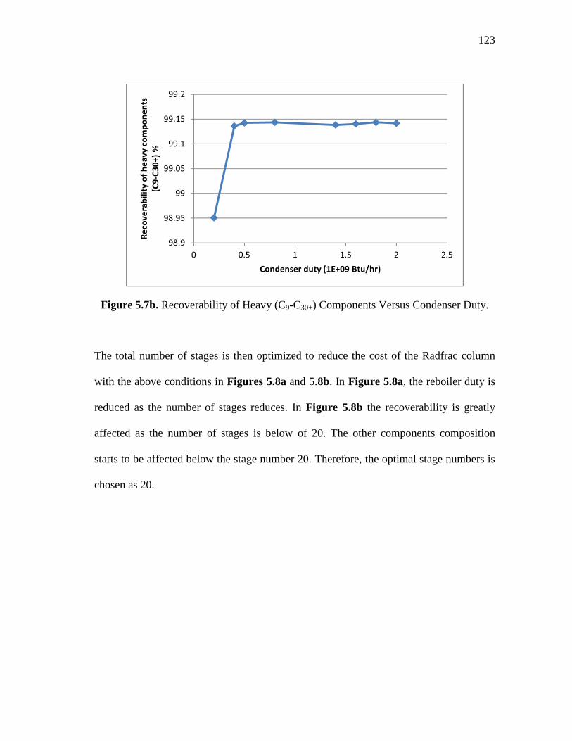
123
Figure 5.7b. Recoverability of Heavy (C9-C30+) Components Versus Condenser Duty.
The total number of stages is then optimized to reduce the cost of the Radfrac column
with the above conditions in Figures 5.8a and 5.8b. In Figure 5.8a, the reboiler duty is
reduced as the number of stages reduces. In Figure 5.8b the recoverability is greatly
affected as the number of stages is below of 20. The other components composition
starts to be affected below the stage number 20. Therefore, the optimal stage numbers is
chosen as 20.
98.9
98.95
99
99.05
99.1
99.15
99.2
0 0.5 1 1.5 2 2.5
Re
cov
era
bil
ity
of
he
av
y c
om
po
ne
nts
(C9
-C3
0+
) %
Condenser duty (1E+09 Btu/hr)

124
Figure 5.8a. Reboiler Duty Versus the Total Number of Stages.
Figure 5.8b. Recoverability of Heavy (C9-C30+) Components Versus the Total Number of Stages.
7.49
7.5
7.51
7.52
7.53
7.54
7.55
7.56
7.57
7.58
0 5 10 15 20 25 30 35
Re
bo
ile
r d
uty
(1
E+
08
Btu
/hr)
Total number of stages
98.5
98.6
98.7
98.8
98.9
99
99.1
99.2
0 5 10 15 20 25 30 35
Re
cov
era
bil
ity
of
he
av
y c
om
po
ne
nts
(C9
-C3
0+
) %
Total number of stages

125
The product streams from the FT reactor could be separated with flash columns first to
reduce the capacity of the stream and to reduce the operation burden and cost burden of
later steps. The separation could be conducted by dropping the pressure and
temperatures of the columns. The sequence of the columns could be operated in two
ways shown in Figures 5.9a and 5.9b. In Figure 5.9a, it is primarily to drop the
pressures of the columns and in Figure 5.9b it is primarily to drop the temperatures of
the columns.
Figure 5.9a. Combination of the Flash Columns with Dropping Pressures.
FTPRO 1
23
4
5
7F1
F2
F3
B5
6

126
Figure 5.9b. Combination of Flash Columns with Dropping Temperatures.
The combination of the operating conditions of the three columns is shown in Table 5.2.
Condition 1 and 2 are standing for the condition in Figures 5.9b, and other conditions
stand for Figure 5.9a.
FTPRO 1
2
3
4
5
7
F1
F2
F3
B5
6

127
Table 5.2. The Conditions of the Three Columns.
Column 1 Column 2 Column 3
Condition T
(°C)
P
(
b
a
r
)
T
(°C)
P
(
b
a
r
)
T
(
°
C
)
P (bar)
1 220 45 200 45 180 45
2 230 45 220 45 210 45
3 200 45 200 40 200 35
4 200 45 200 40 200 30
5 200 45 200 35 200 30
6 200 45 200 35 200 25
7 220 45 220 35 220 30
8 210 45 210 35 210 30
9 190 45 190 35 190 30
10 180 45 180 35 180 30
11 190 45 190 35 190 25
12 180 45 180 35 180 25
13 180 45 180 30 180 20
14 160 45 160 30 160 15
The analysis result is shown in Figures 5.10a and 5.10b. Condition 1 and 2 from
Figures 5.9b are not the optimum choices because the recovered flow rate is high, which
increases the later steps cost. The choices are focused on the combination in Figure 5.9a.
The requirements should be high for heavy components recoverability and low for
recovered flow rate. This way, the results in the two figures give the choices in condition
4, 5, 11, and 13; and in this work, condition 5 is used for later steps.

128
Figure 5.10a. Recoverability of Heavy (C9-C30+) Components Versus Pressure and Temperature Conditions of the Flash Columns.
Figure 5.10b. Recovered Heavy Components Flow Rate Versus the Pressure and Temperature Conditions of the Flash Columns.
84
86
88
90
92
94
96
98
100
102
0 2 4 6 8 10 12 14 16
He
av
y c
om
po
ne
nts
(C
9-C
30
+)
reco
ve
rab
ilit
y (
%)
condition number
0
20000
40000
60000
80000
100000
120000
140000
160000
0 2 4 6 8 10 12 14 16
Re
cov
ere
d f
low
ra
te (
lbm
ol/
hr)
condition number

129
From this analysis, the molar recoverability of heavy components increases from 98.8%
to 99.2% and it does not influence the recovering of other components. At the same time,
external utility and column cost are reduced.
The part of recovering light fractions process is conducted in the following. The Radfrac
column 2 is replaced with a flash column to analyze the effect. The result of simulation
shows that the recovered pergas and solvent streams are not affected greatly, while at the
same time the energy cost of the flash column reduces significantly. Then, the flash
column 4 is added with a condenser after it to increase the purity and recovery of the
pergas stream. The simulation result shows that the overall recovery of pergas increases
from 98.9% to 99.2% and the solvent recoverability increases from 97.4% to 99.9%
while the external energy consumption reduces.
An economic analysis was carried out with the software Aspen Icarus and the results are
shown in Table 5.3, notice that the fixed cost is composed of direct and indirect cost
based on all the equipment cost in the process from the simulation result. The case with
Radfrac column installed has the highest cost, and the case with heavy column adjusted
has the lowest fixed cost. The heat balance of each scenario is identified and heat
integration is carried out and optimized using the software Lingo to yield a heating
utility cost of 3$/MMBtu and cooling utility cost of 5$/MMBtu. The main results for the
heat integration are shown in Table 5.4, notice that the case with heavy component

130
separation optimized is the one with the minimum utility costs, whereas the case with
the radfrac column is the one with the highest utility costs.
The mass balance of the separation result for each scenario is identified and then the
mass integration is carried out. For the process economic analysis, the following unit
costs were used, syngas $13/GJ, hexane $1.15/gal, diesel $82/bbl, gasoline $63/bbl, H2
$2/kg, H2O $1.2x10⁻³/gal, tailgas $50/bbl. The cost analysis is shown in Table 5.5. The
result shows that the case with heavy column optimized has the highest return of
investment. While the case with the condenser added has the highest recoverability and
purity, and the case with the flash sequence optimized has the highest sale of production.
The case with the Radfrac column replaced has the highest energy saved. This
information is very useful, because this allows to the designer to choose the best case
dependent on the objective of the design.

131
Table 5.3. Fixed Cost (US$) for Different Scenarios Analyzed.
Unit with condenser with no condenser replace radfrac flash sequence heavy column
flash column1 30,844,719 30,844,719 30,844,719 34,732,760 30,844,719
flash column2 29,623,455 29,623,455 29,623,455 3,948,988 29,623,455
flash column3 22,368,446 22,368,446 22,368,446 1,701,861 22,368,446
flash column4 844,882 844,882 844,882 844,882 844,882
radfrac
distillation 1
483,388,081 483,388,081 483,388,081 483,388,081 428,024,094
radfrac
distillation 2
5,911,850 5,911,850 58,159,170 5,911,850 5,911,850
radfrac
distillation 3
69,822,826 69,822,826 69,822,826 69,822,826 69,822,826
FT synthesis 680,335,917 680,335,917 680,335,917 680,335,917 680,335,917
heat exchanger1 4,195,567 4,195,567 4,195,567 4,195,567 4,195,567
heat exchanger2 9,759,880 9,759,880 9,759,880 9,759,880 9,759,880
heat exchanger3 1,068,199 1,068,199 1,068,199 1,068,199 1,068,199
heat exchanger4 3,632,622 3,632,622 3,632,622 3,632,622 3,632,622
heat exchanger5 3,632,622 3,632,622 3,632,622 3,632,622 3,632,622
pump 2,605,364 2,605,364 2,605,364 2,605,364 2,605,364
131

132
132
Table 5.3. Continued
condenser1 1,268,254 - - - -
condenser2 754,625 754,625 754,625 754,625 754,625
total 1,350,057,309 1,348,789,055 1,401,036,374 1,306,336,043 1,293,425,069
Table 5.4. Results Comparison for The Energy Consumption.
Case Hot utility
requirement
(BTU/hr)
Cold utility
requireme
nt
(BTU/hr)
Cost for hot
utility
(MM$/yr
)
Cost for cold
utility
(MM$/yr
)
Total utility
cost
(MM$/y
r)
With condenser added 0.1039885E+11 0.1678697E+11 288 776 1064.023
With no condensed added 0.1039885E+11 0.1678697E+11 288 776 1064.023
with heavy components
separation optimized
0.8619653E+10 0.1528577E+11 239
706
945.322
with flash sequence optimized 0.1139260E+11 0.1582207E+11 316 730 1046.911
With Radfrac column 0.1084365E+11 0.1750977E+11 301 808 1109.746
132

133
133
Table 5.5. Cost Analysis of Five Scenarios Analyzed.
Case/concept With
conde
nser
With no
condens
er
Replace
radfr
ac
Flash
sequence
Heavy
colum
n
Annual capital cost (MM$/yr) 61 61 63 59 58
Annual operating cost (MM$/yr) 3,017 3,056 3,231 2,863 2,836
Utility cost without heat integration (MM$/yr) 1,715 1,715 1,880 1,530 1,592
Utility cost with energy integration(MM$/yr) 1,064 1,064 1,110 1,047 945
Total sales(MM$/yr) 3,619 3,619 3,619 3,621 3,611
ROI without energy integration 0.29 0.28 0.19 0.38 0.39
ROI with energy integration 0.60 0.58 0.54 0.62 0.71
133

134
Overall, for the cases analyzed, the permenant gas has been separated from solvent
stream with 99% of recoverability, the solvent has been separated with 99% of
recoverability, and the heavier components product has been recovered with 99% of
recoverability, and the recovery of the components is shown in Figure 5.11, where the x
axis shows the components from carbon 1 to carbon 31, water, H2 and CO, and the y
axis shows the recoverability of the component. There are 8 series showing 8 output
streams, including water streams, solvent streams, permenant gas streams, and heavier
components streams. The graph shows that 99% of water is recovered in the water
stream, 99% of solvent (C5-C8) is recovered in the solvent stream, 99% of C9+
components is recovered in the heavier stream, and 99% of the C1-C4 is recovered in the
pergas stream.
Figure 5.11. Recovery of the Components in Each Stream.
0%
10%
20%
30%
40%
50%
60%
70%
80%
90%
100%
1 4 7 10 13 16 19 22 25 28 31
reco
vera
bili
ty
component
Recoverability of each component in the streams
WATER2
WATER1
HEAVY
SOLVENT3
SOLVENT2
SOLVENT1
PERGAS2
PERGAS1

135
5.6.3 Economic Evaluation to Compare the SCF-FT and Conventional FT
Process
The optimum scenario of the abovementioned separation design is included in the SCF-
FT process to compare the cost potential with conventional FT process on the GTL basis.
The major parts included in calculating the fixed cost are shown in Figure 5.12. Results
show that although GTL with SCF-FT design has higher cost due to the installation of
the pressure compression units and solvent separation units, it could be more energy
efficient in utilizing the pressure and temperature when separating, and in this way the
overall return of investment of GTL is higher than the conventional process. This means
that the GTL process with supercritical solvent design is competitive.
Figure 5.12. Process Units in the GTL Process.

136
The costs calculation for the components of the units is based on the literature reports of
the NETL (Kreutz et al., 2008) using the corresponding scaling factor in addition to
Aspen Icarus estimations. The equipment cost is calculated using the following scaling
methods from the existing cost case. The train capacity is calculated as S=Sr/n,
C=C0×(S/S0)f, Cm=C×nm, where Cm is the component cost, C is the train cost, Sr is the
required capacity, S is the train capacity, S0 is the base capacity, n is the train number,
C0 is the base cost reported, f is the scaling factor and m was assumed as 0.9. Project
contingencies were added to cover project uncertainty and the cost of any additional
equipment that could result from a detailed design. For typical chemical plants, the
OSBL costs are only 20% of the ISBL costs. However, in a GTL plant the volumes of
the side streams are very high (i.e. the oxygen and nitrogen from the ASU as well as
water by-product from the FT synthesis) and handling and treatment of these streams
require correspondingly more auxiliary operations (Richardson, 1993).
Table 5.6 shows a results comparison for the traditional FT process optimized in this
paper respect to the SCF-FT process proposed in this paper. Notice that the capital cost
for the SCF-FT respect to the traditional FT process increases 36%, the operational costs
decreases 9% and the total sales increase 5%; as a results the ROI increase from 0.25 to
0.26 for the SCF-FT process proposed in this paper respect to the traditional FT process
optimized using the strategy proposed in this paper.

137
Table 5.6. Economic Comparison for the Traditional and SCF FT Processes.
Process Total capital Cost
(MM$) Total Operational cost
(MM$/yr) Total Sales (MM$/yr)
ROI
Traditional FT process 3248 5203 7493 0.25
SCF-FT process 4406 4730 7826 0.26
The comparison of $/BPD of this case is compared with current GTL processes shown in
Table 5.7, and the unit cost of each major part is shown in Table 5.8. The data show that
the capital investment per BPD of the proposed case is a little higher than the existing
plant of GTL and it is within the range of the typical cost trend. The cost distribution of
this case is compatible with the typical GTL cost distribution of each major part. In this
case, the upgrading cost is a little higher than typical case, indicating the cost related
with the gas recovery and additional installation of solvent recovery system.
Table 5.7. Total Capital Investment (TCI) of the Process.
Plant BPD TCI (MM$) $/BPD
Bintulu (Shell) 12,500 850 68,000
Oryx (Sasol) 34,000 1,100 32,353
Nigeria (Sasol) 34,000 2,000 58,824
This case 120,000 10,718 89,320

138
Table 5.8. The Distribution of the Cost of the GTL Process.
UNIT Typical case (%) This case (%)
ASU 30 27
syngas manufacture 30 17
FT 25 20
upgrading 15 21
power 0 15
5.7 Conclusions
In this work the performance of supercritical solvent separation from Fischer-Tropsch
products has been evaluated. An approach has been proposed to recover solvent from
SCF-FT products. A process for recovering is developed followed by optimization and
heat integration to analyze the economic potential. A flowsheet is established for
separation of the products. A case study is implemented to optimize the efficiency of
separating and the effect of products. Alternative scenarios for supercritical solvent
separation for FT products have been investigated and selected based on the developed
mathematic model. A comparison of cost efficiency between common FT process and
SCF-FT process has been carried out, and the result shows that SCF-FT is competitive to
conventional GTL processes when supercritical operation is coupled with proper
separation designs.

139
6. SUMMARY, CONCLUSIONS AND FUTURE WORK
In this work, a shortcut method has been introduced for the conceptual design and
preliminary synthesis of alternative pathways of the process industries with focus on the
applications for biorefineries. The chemical species/conversion operator structural
representation has been introduced. It tracks chemical species, connects various streams
with processing technologies, and embeds potential configurations of interest. An
optimization formulation has been developed to maximize the yield or the economic
potential subject to constraints that include process models, distribution of streams and
species over the conversion technologies, interconnection of the candidate technologies,
and techno-economic data. Three case studies have been solved to demonstrate the
effectiveness and applicability of the developed approach. The case studies covered the
scenarios of maximum theoretical yield, accounting for actual process yield, including
more than one feedstock, and incorporating an economic objective (payback period),
The solutions of the case study illustrate the ability of the proposed approach to generate
a wide variety of pathways that achieve the same target but vary significantly in their
building blocks and interconnections. The solution of the case studies also demonstrates
that by including an economic objective function that the complexity of the devised
pathways is greatly reduced.
Also, in this work a system to effectively optimize a biorefinery technology pathway
integrated with species separation and recycle networks has also been developed.

140
The synthesis and design of separation networks has also been studies for a supercritical
fluid Fischer-Tropsch (SCF FT) gas-to-liquid (GTL) process. . A solvent-recovery
process has been synthesized. Optimization and heat integration have been employed to
improve the economic performance of the process. A case study has been solved to
include and screen alternative scenarios for supercritical solvent separation. A
comparison of cost efficiency between common FT process and SCF-FT process has
been carried out. The results show that the SCF-FT is competitive with conventional
GTL processes when the supercritical operation is coupled with proper separation
designs.
The following research activities are proposed for future work:
• Inclusion of fluctuation in the feedstock quality in the synthesis procedure for
biorefineries (design under uncertainty).
• Integration of process design and operation for biorefineries.
• Inclusion of process safety as an objective in the design of biorefineries.
• Assessment of different solvents for SCF FT and analysis of techno-economic
factors for the various solvents.

141
REFERENCES
Adsul, M., Khire, J., Bastawde, K. and Gokhale, D. 2007. Production of lactic acid from
cellobiose and cellotriose by Lactobacillus delbrueckii Mutant Uc-3. Applied
Environmental Microbiology. 75(15), 5055-5057.
Aiello-Mazzarri, C., Agbogbo, F.K. and Holtzapple, M.T., 2006. Conversion of
municipal solid waste to carboxylic acids using a mixed culture of mesophilic
microorganisms. Bioresource Technology, 97, 47-56.
Alcohol solutions, 2001. Renewable methanol and liquid carbon dioxide from landfill
gas. Available at http://www.methanol.org/pdf/MethanolfromLFGBrochure.pdf
Alden, R.C., 1946. Conversion of natural gas to liquid fuels. The Oil and Gas Journal, 9,
79-98.
Alvarado-Morales, M., Terra, J., Gernaey, K.V., Woodley, J.M., Gani, R., 2009.
Biorefining: Computer aided tools for sustainable design and analysis of bioethanol
production. Chemical Engineering Research and Design, 87, 1171-1183.
Anderson, R.B., 1956. Catalysis, Emmett (ed.) Reinhold, New York.
Askew, M., 2005. The biorefinery concept.
http://europa.eu.int/comm/research/energy/pdf/renews3.pdf
Azapagic, A., 2002. Sustainable development progress metrics. IChemE Sustainable
Development Working Group, IChemE Rugby, UK

142
Bagajewicz, M., 2000. A review of recent design procedures for water networks in
refineries and process plants. Computers and Chemical Engineering, 24(9-10), 2093-
2113.
Baldwin, T.D., Stinson, J. and Ham, R.K., 1998. Decomposition of specific materials
buried within sanitary landfills. Journal of Environmental Engineering, 124, 1193–1202.
Bao, B., Ng, D.K.S., Tay, D.H.S., Jiménez-Gutiérrez, A., El-Halwagi, M.M., 2011. A
shortcut method for the preliminary synthesis of process-technology pathways: An
optimization approach and application for the conceptual design of integrated
biorefineries. Computers and Chemical Engineering, 35, 1373-1384.
Bao, B., El-Halwagi, M.M., El-Bashir, N.O., 2010a, Simulation, integration and
economic analysis of gas-to-liquid process. Fuel Processing Technology, 91 (7), 703-713.
Bao, B., El-Bashir, O.N., El-Halwagi, M.M., 2010b, Techno-economic analysis of gas-
to-liquid process. Proceedings of the 2nd Annual Gas Processing Symposium, edited by
Benyahia F. and Eljack, F., Series “Advances in Gas Processing”, Gas Processing Center,
Doha, January 2010.
Bartholomew, C.H., and Farrauto, R.J., 2006, Fundamentals of Industrial Catalytic
Processes. Second ed., Hoboken: Wiley & Sons.
Bechtel, 1992. Baseline design/economics for advanced Fischer-Tropsch technology.
Quarterly Report, Jan-Mar.
Bechtel, 1998a. Baseline design/economics for advanced Fischer-Tropsch technology.
Report under contract DEAC22- 91PC90027, Federal Energy Technology Center.

143
Bechtel, 1998b. Aspen process flowsheet simulation model of a Battelle biomass-based
gasification, Fischer-Tropsch liquefaction and combined-cycle power plant, DE-AC22-
93PC91029-16. US Dept. of Energy, Pittsburgh, Pennsylvania, May.
Benko, N., Rev, E., Fonyo, Z., 2000. The use of nonlinear programming to optimal
water allocation. Chemical Engineering Communications, 178, 67-101.
Bioenergy, IEA, 1998. The Role of Bioenergy in Greenhouse Gas Mitigation.
Bochniak, D.J, Subramaniam, B., 1998, Fischer-Tropsch synthesis in near critical n-
hexane: pressure-tuning effects. AIChE Journal, 44,1889–1896.
Boerrigter. H., 2006. Economy of biomass-to-liquids (BTL) plants. An Engineering
Assessment
Bolder, F.H.A., and Mulder, H., 2005. Dehydration of alcohols in the presence of
carbonyl compounds and carboxylic acids in a Fsischer-Tropsch hydrocarbons matrix.
Applied Catalysis A: General. 300, 36-40.
Bordawekar M, Roberts CB, editors. 2007. Effects of Super-Critical Fluid Extraction on
the Activity and Selectivity of Fischer Tropsch Catalysts. Preprints of Symposia.
Washington, DC: Division of Fuel Chemistry, American Chemical Society.
Bridgwater, A.V., 2003. Renewable fuels and chemicals by thermal processing of
biomass. Chemical Engineering Journal, 91 (2-3), 87-102.
Bridgwater T., 2008. Biofuel production. Available at
http://www.omega.mmu.ac.uk/Alternative-Fuels-
Presentations/Tony%20Bridgwater%20Aston%20University%20-
%20Biofuel%20Production.pdf

144
Bringezu, S., Schutz, H., O’Brien, M., Kauppi, L., Howarth, W.R., 2009. Towards
sustainable production and use of resources: Assessing biofuels. United Nations
Environment Programme. 10-16.
Caldwell, L., van Vuuren, D.S., 1986. The formation and composition of the liquid
phase in Fischer-Tropsche reactors. Chemical Engineering Science, 41, 89-96.
Chakraborty, A., 2009. A globally convergent mathematical model for synthesizing
topologically constrained water recycle networks. Computers and Chemical Engineering,
33(7), 1279-1288.
Chen, W., Ding, Y., Jiang, D., Wang, T., Luo, H., 2006. A selective synthesis of acetic
acid from syngas over a novel Rh nanoparticles/nanosized SiO2 catalysts. Catalysis
Communications, 8, 559-562.
Chouinard-Dussault, P., Bradt, L., Ponce-Ortega, J.M., El-Halwagi, M.M., 2011.
Incorporation of process integration into life cycle analysis for the production of biofuels.
Clean Technologies and Environmental Policy, 13(5), 673-685.
Costa, E., Ugulna, A., Aguado, J. and Herndndez, P.J., 1985. Ethanol to gasoline process:
Effect of variables, mechanism, and kinetics. Industrial and Engineering Chemistry
Process Design and Development, 24, 239-244.
Davis, B.H., 2003. Fischer-Tropsch synthesis: supercritical conversion using a Co/Al2O3
catalyst in a fixed bed reactor. Fuel, 82,1251–1260.
Department of the Environment., 1995. Landfill design, construction and operational
practice. Waste management paper, 26B, Her Majesty’s Stationery Office, London.

145
Dhole, V.R., Ramchandani, N., Richard, A.T., Marek, W., 1996. Make your process
water pay for itself. Chemical Engineering, 103(1), 100-103.
Dong, K.K., Chang, Y.C., Woo, T.L., Jong, H.K., 2001. Microwave dehydrogenation of
ethane to ethylene. Journal of Industrial and Engineering Chemistry, 7, 363-374.
Douglas, J.M., 1988. Conceptual Design of Chemical Processes. New York, McGraw
Hill.
Dry, M.E., 1996. Practical and theoretical aspects of catalytic Fischer-Tropsch process.
Applied Catalyst A: General, 138, 319-344.
Dunn, R.F., Wenzel, H., Overcash, M.R., 2001a. Process integration design methods for
waste conservation and wastewater reduction in industry: Part I. Design for multiple
contaminants. Clean Products and Processes, 3, 319-329.
Dunn, R.F., Wenzel, H., Overcash, M.R., 2001b. Process integration design methods for
waste conservation and wastewater reduction in industry: Part I. Design for single
contaminants. Clean Products and Processes, 3, 307-318.
Durham, E., Zhang, S., Roberts, C.B., 2008. Supercritical reactivation of Fischer
Tropsch catalysts. AIChE Annual Meeting: Presentation 678d. In: Durham E
EIA, Energy Information Administration 2010. International Energy Outlook 2010.
http://www.eia.gov/oiaf/ieo/world.html.
Eilers, J., Posthuma, S.A., Sie, S.T., 1990. The shell middle distillate synthesis process
(SMDS). Catalysis Letters, 7, 253-270
El-Bashir, N.O., Roberts, C.B., 2005. Enhanced incorporation of a-olefins in the Fischer-
Tropsch synthesis chain-growth process over an alumina supported cobalt catalyst in

146
near-critical and supercritical hexane medium. Industrial and Enginering Chemistry
Research, 44, 505–521.
El-Bashir, N.O., Bao, B., El-Halwagi, M.M., 2009. An approach to the design of
advanced Fischer-Tropsch reactor for operation in near-critical and supercritical phase
media. Proceedings of the 1st Annual Gas Processing Symposium, Alfadala, H., Rex
Reklaitis, G.V. and El-Hawagi, M.M. (Editors), Doha.
El-Bashir, N.O., Bukur, D.B., Durham, E., Roberts, C.B., 2010. Advancement of
Fischer-Tropsch synthesis via utilization of supercritical fluid reaction media. AIChE
Journal, 56 (4), 997-1015.
El-Halwagi, M.M. 1997. Pollution Prevention Through Process Integration. Academic
press, San Diego
El-Halwagi, M.M. 2006. Process Integration, volume 7. Academic press, San Diego
El-Halwagi, M.M., Glasgow, I.M., Qin, X., 2004. Property integration: Componentless
design techniques and visualization tools. AIChE Journal, 50(8), 1854-1869.
El-Halwagi, M.M., Hamad, A.A., Garrison, G.W., 1996. Synthesis of waste interception
and allocation networks. AIChE Journal, 42(11), 3087-3101.
El-Halwagi, M.M., and Manousiouthakis, V., 1989. Synthesis of mass exchange
networks. AIChE Journal, 35(8), 1233-1244.
El-Halwagi, M.M., and Spriggs, H.D., 1998. Solve design puzzles with mass integration.
Chemical Engineering Progress, 94(8), 25-44.

147
Elms, R.D. and El-Halwagi, M.M., 2009. Optimal scheduling and operation of biodiesel
plants with multiple feedstocks. International Journal of Process Systems Engineering, 1,
1–28.
EPRI-Electric Power Research Institute, 1993. Technical Assessment Guide (TAG)
Electricity Supply, TR-102276-V1R7, EPRI, Palo Alto, California.
Espinoza, R.L., Steynberg, A.P., Jager, B., Voslo, A.C., 1999. Low temperature Fischer-
Tropsch synthesis from a Sasol perspective. Applied Catalysis A: General, 186, 13-26.
Fan, L., Yokota, K., Fujimoto, K., 1992. Supercritical phase Fischer-Tropsch synthesis:
catalyst pore-size effect. AIChE Journal, 38, 1639-1648.
Ferdinand, L and Arthur, H., 1994. Preparation of formic acid from carbon monoxide
and water. US Patent No: 5334759. Available at:
http://www.freepatentsonline.com/5334759.pdf
Fernando, S., Adhikari, S., Chandrapal, C., Murali, N., 2006. Biorefineries: Current
status, challenges, and future directions. Energy and Fuels, 20(4), 1727–1737.
Filippis, P., Borgianni, C., Paolucci, M., Pochetti, F., 2004. Prediction of syngas quality
for two-stage gasification of selected waste feedstocks. Waste management, 24, 633-639.
Fincke, J., Anderson, R., Hyde, T., Wright, R., Bewley, R., 2000. Thermal conversion of
methane to acetylene final report. Idaho National Engineering and Environmental
Laboratory
Foo, D.C.Y., Kazantzi, V., El-Halwagi, M.M., Manan Z.A., 2006. Surplus diagram and
cascade analysis technique for targeting property-based material reuse network.
Chemical Engineering Science, 61(8), 2626-2642.

148
Fox, J.M., and Tam, S.S., 1995. Correlation of slurry reactor Fischer-Tropsch yield data.
Topics in Catalysis, 2, 285-300.
Fu, X., Zhu, B., Tian, S., Hou, S., Long, J., 2007. Decarboxylation technology for
processing high acid crude via fluid catalytic cracking. JCK oil meeting. Available at
http://www.pecj.or.jp/japanese/plaza/china/JCKoilmeeting20071203/a-4.pdf
Gabriel, F.B. and El-Halwagi, M.M., 2005. Simultaneous synthesis of waste interception
and material reuse networks: Problem reformulation for global optimization.
Environmental Progress, 24(2), 171-180.
Garrard, A., and Fraga, E.S., 1998. Mass exchange network synthesis using genetic
algorithms. Computers and Chemical Engineering, 22(12), 1837-1850.
Gomes, J.F.S., Queiroz, E.M., Pessoa, F.L.P., 2007. Design procedure for
water/wastewater minimization: single contaminant. Journal of Cleaner Production, 15
(5), 474-485.
Gosling, I., 2005. Process simulation and modeling for industrial bioprocessing: tools
and techniques. Industrial Biotechnology, 1(2), 106–109.
Gould, Ronald, Yurchak, Sergei, 1982. Method for gasoline yield enhancement in the
fixed bed methanol-to-gasoline process. United States Patent 4523046.
Goyal, H.B., Diptendu, S., and Saxena, R.C., 2008. Bio-fuels from thermochemical
conversion of renewable resources: A review. Renewable and Sustainable Energy
Reviews. 12, 504-517.

149
Grooms, D., Kazantzi, V., El-Halwagi, M.M., 2005. Optimal synthesis and scheduling of
hybrid dynamic/steady-state property integration networks. Computers and Chemical
Engineering, 29(11-12), 2318-2325.
Hackett, C., Williams, R. B., Durbin, T. D., Welch, W., Pence, J., Aldas, R., Jenkins, B.
M., and Salour, D., 2004. Evaluation of conversion technology processes and products.
Draft final Report, University of California.
Ham, R.K., Norman, M.R. and Fritschel, P.R., 1993. Chemical characterization of fresh
kills landfill refuse and extracts. Journal of Environmental Engineering, 119, 1176–1195.
Hamelinck, C.N. and Faaij, A.P.C, 2002. Future prospects for production of methanol
and hydrogen from biomass. Journal of Power Sources, 111(1), 1-22.
He, M., Hu, Z., Xiao, B., Li, J., Guo, X. and Luo, S., 2008. Hydrogen-rich gas from
catalytic steam gasification of municipal solid waste (MSW): Influence of catalyst and
temperature on yield and product composition. International Journal of Hydrogen
Energy, 9, 1-9.
Holtzapple, M.T., Davison, R.R., Ross, M.K., Aldrett-Lee, S., Nagwani, M., Lee, C.M.,
Lee, C., Adelson, S., Kaar, W., Gaskin, D., Shirage, H., Chang, N., Chang, V. and
Hon, Y., How, L., Mat, Y., Ahmad, I., 2001. Separation of water-oil emulsion by using
membrane. 15th symposium of Malaysian chemical engineers SOMCHE.
Huang, X., and Roberts, C.B., 2003. Selective Fischer-Tropsch synthesis over an Al2O3
supported cobalt catalyst in supercritical hexane. Fuel Processing Technology, 83,81–99.
Huber, G.W., Iborra, S., Corma, A., 2006. Synthesis of transportation fuels from
biomass: Chemistry, catalysts, and engineering. Chemical Reviews, 106(9) 4044-4098.

150
IEA, International Energy Agency, 2010. World Energy Outlook 2010.
Ivannova, L.K., Richads, D.J., Smallman, D.J., 2008. Assessment of the anaerobic
biodegradation potential of MSW. Proceedings of the Institution of Civil Engineers,
Waste and Resource Management, 161, 167-180.
Jacobs, G., Chaudhari, K., Sparks, D., Zhang, Y., Shi, B., Spicer, R., Das, T.K., Li, J.,
Jager, B., and Espinoza, R., 1995. Advances in low temperature Fischer-Tropsch
synthesis. Catal Today. 23,17–28.
Jin, B, Yin, P, Ma, Y. and Zhao, L.. 2005. Production of lactic acid and fungal biomass
by Rhizopus fungi from food processing waste streams. Journal of Industrial
Microbiology and Biotechnology, 32 (1), 678–686.
John, S.P., 2004. System and method for treatment of water and disposal of
contaminants produced by converting lighter hydrocarbons into heavier hydrocarbon.
Patent 6794417.
Jones, S,B., Holladay, J.E., Valkenburg, C., Stevens, D.J., Walton, C.W., Kinchin, C.,
Elliott, D.C., Czernik,S., 1999. Production of gasoline and diesel from biomass via fast
pyrolysis, hydrotreating and hydrocracking: A design case. A report prepared by US
Department of Energy.
Jones, S.B., Zhu, Y., Valkenburg, C., 2009. Municipal solid waste (MSW) to liquid fuels
synthesis, Volume 2: A techno-economic evaluation of the production of mixed alcohols.
US Department of Energy.
Kazantzi, V., El-Halwagi, M.M., 2005. Targeting material reuse via property integration.
Chemical Engineering Progress, 101(8), 28-37.

151
Kazantzi, V., Qin, X.Y., El-Halwagi, M.M., Eljack, F., Eden, M., 2007. Simultaneous
process and molecular design through property clustering techniques: A visualization
tool. Industrial and Engineering Chemistry Research, 46(10), 3400-3409.
Khanmetov, A., Azizov, A., Piraliev, A., 2006. Ethylene oligomerization in the presence
of catalyst systems based on mixed ligan b-diketonatoziroconium chlorides. Petroleum
Chemistry, 46, 366-370.
Knifton, J., 1985. Syngas reaction IX. Acetic acid from syntheis gas. Journal of Catalysis,
96, 439-453.
Kokossis, A.C., and Yang, A., 2009. Future system challenges in the design of
renewable bio-energy system and the synthesis of sustainable biorefineries. Proceeding
of Seventh International Conference on Foundations of Computer-Aided Process Design,
207-2011.
Kreutz, T., Williams, R., Consonni, S., and Chiesa, P., 2005. Co-production of hydrogen,
electricity and CO2 from coal with commercially ready technology. Part B: Economic
analysis. International Journal of Hydrogen Energy, 30, 769-784.
Kreutz, T.G., Larson, E.D., Liu, G., Williams, R.H., 2008. Fischer-Tropsch fuels from
coal and biomass. 25th Annual International Pittsburgh Coal Conference. Pittsburgh,
Pennsylvania.
Krishnan, M. S., Ho, N.W.Y., and Tsao, G.T., 1999. Fermentation kinetics of ethanol
production from glucose and xylose by recombinant saccaromyces 1400 (pLNH33).
Applied Biochemistry and Biotechnology, 78(1-3), 373-388.

152
Kusmlyati, N.A.S., 2007. Conversion of methane to gasoline range hydrocarbons over
W/HZSM-5 catalyst: Effect of co-feeding. Available at
http://eprints.utm.my/5086/1/Kusmiyati2007_ConversionOfMethaneToGasolineRange.p
df
Loescher, M.E, 1999. Biomass conversion to mixed alcohol fuels using the MixAlco
process. Applied Biochemistry and Biotechnology, 79(1-3), 609-631.
Lynd, L.,R., 1996. Overview and evaluation of fuel ethanol from cellulosic biomass:
Technology, economics, the environment, and policy. Annual Review of Energy and the
Environment, 21, 403-465.
Manan, Z.A., Tan, Y.L., Foo, D.C.Y., 2004. Targeting the minimum water flow rate
using water cascade analysis technique. AIChE Journal, 50(12), 3169-3183.
Mansoornejad, B., Chambost, V., Stuart, P., 2009. Integrating product portfolio design
and supply chain design for the forest biorefinery. Proceeding of Seventh International
Conference on Foundations of Computer-Aided Process Design, 1017-1033.
Micales, J.A. and Skog, K.E., 1997. The decomposition of forest products in landfills.
International Biodeterioration and Biodegradation, 39, 145–158.
Minowa, T., Murakami, M., Dote, Y., Ogi, T. and Yokoyama, S., 1995. Oil production
from garbage by thermochemical liquefaction. Biomass and Bioenergy. 8, 117-120.
Mohan, T., and El-Halwagi, M.M. 2007. An algebraic targeting approach for effective
utilization of biomass in cogeneration systems through process integration. Journal of
Clean Technology and environmental Policy, 9(1), 13-25.

153
Morello, J., and Pate, R., 2010. The promise and challenge of algae as renewable sources
of biofuels. Biomass program webinar
Myint, L.L., and El-Halwagi, M.M., 2009. Process analysis and optimization of
biodiesel production from soybean oil. Clean Technologies and Environmental Policy,
11(3), 263-276.
Murphy, J.D. and McCarthy, K.. 2005. Ethanol production from energy crops and wastes
for use as a transport fuel in Ireland. Applied Energy. 82(2), 148-166.
Napoles-Rivera, F., Ponce-Ortega, J.M., El-Halwagi, M.M., Jimenez-Gutierrez, A., 2010.
Global optimization of mass and property integration networks with in-plant property
interceptors. Chemical Engineering Science, 65(15), 4363-4377.
National Renewable Energy Laboratory (NREL), 2005. Conceptual biorefinery.
Available from http://www.nrel.gov/biomass/biorefinery.html
NETL- National Energy Technology Laboratory, 2007. Cost and performance baseline
for fossil energy plants: Volume 1: Bituminous Coal and Natural Gas to Electricity.
DOE/ NETL-2007/1281, Rev. 1, August (www.netl.doe.gov).
Ng, D.K.S., Pham, V., El-Halwagi, M.M., Jiménez-Gutiérrez, A. and Spriggs, H.D.,
2009. A hierarchical approach to the synthesis and analysis of integrated biorefineries.
Proceeding of Seventh International Conference on Foundations of Computer-Aided
Process Design 2009, 425-432.
Ng, D.K.S., 2010. Automated targeting for synthesis of an integrated biorefinery.
Chemical Engineering Journal, 162 (1), 67–74.

154
Ng, D.K.S., Foo, D.C.Y., Tan, R.R., 2007a. Targeting for total water network. 1. Waste
stream identification. Industrial and Engineering Chemistry Research, 46(26), 9107-
9113.
Ng, D.K.S., Foo, D.C.Y., Tan, R.R., 2007b. Targeting for total water network. 2. Waste
treatment targeting and interactions with water system elements. Industrial and
Engineering Chemistry Research, 46(26), 9114-9125.
Nishida, N., Stephanopoulos, G., Westerberg, A.W., 1981. A Review of Process
Synthesis. AIChE Journal, 27(3), 321-351.
NREL, National Renewable Energy Laboratory, 2005. Conceptual biorefinery.
http://www.nrel.gov/biomass/biorefinery.html.
NREL, 2007. Municipal solid waste in the United States: 2007 Facts and Figures
Ogden, J.M., 2004. Conceptual design of optimized fossil energy systems with capture
and sequestration of carbon dioxide. Institute of Transportation Studies, University of
California, Davis, Research Report UCD-ITSRR-04-34.
Ogden, J., 2003. Modeling infrastructure for a fossil hydrogen energy system with CO2
sequestration, in J. Gale and Y Kaya (eds). Proceedings of the 6th International
Conference on Greenhouse Gas Control Technologies, Oxford: Elsevier Science, pp.
1069-74.
Ojolo, S. and Bamgboye, A., 2005. Thermochemical conversion of municipal solid
waste to produce fuel and reduce waste. Agricultural Engineering International: the
CIGR Ejournal. Vol. VII. Manuscript EE 05 006. September, 2005.

155
Perry, R.H., and Green, D., 1984. Perry's Chemical Engineers' Handbook. 6th Ed.,
McGraw-Hill, NY
Peters, M.S., and Timmerhaus, K.D., 1991. Plant Design and Economics for Chemical
Engineers. McGraw-Hill, NY
Pham, V., Holtzapple, M., El-Halwagi, M.M., 2010. Techno-economic analysis of
biomass to fuel conversion via the MixAlco process. Journal of Industrial Microbiol
Biotechnology, 37, 1157-1168.
Phyllis, 2008. Composition of biomass and waste database. Energy Research Centre of
the Netherlands, Petten, Holland, Netherlands. Accessed April 24, 2008 at
http://www.ecn.nl/phyllis
Pierre, G., 2007. Process options for the catalystic conversion of renewables into
bioproducts. In Catalysis for Renewables: From Feedstock to Energy Production, Centi
G. and van Santen R.A. (Edts). Wiley-VCH Verlag, KgaA, Weinheim.
Pillai, H.K., and Bandyopadhyay, S., 2007. A rigorous targeting algorithm for resource
allocation networks. Chemical Engineering Science, 62(22), 6212-6221.
Pokoo-Aikins, G., Nadim, A., El-Halwagi, M.M., Mahalec, V., 2010ba Design and
analysis of biodiesel production from algae grown through carbon sequestration. Clean
Technologies and Environmental Policy, 12(3), 239-254.
Pokoo-Aikinsa, G., Heatha, A., Mentzerb, R.A., Mannanb, M.S., Rogersb, W.J., El-
Halwagi, M.M., 2010b. A multi-criteria approach to screening alternatives for
converting sewage sludge to biodiesel. Journal of Loss Prevention in the Process
Industries, 23(3), 412 – 420.

156
Polley, G.T., and Polley, H.L., 2000. Design better water networks. Chemical
Engineering Progress, 96(2), 47-52.
Ponce-Ortega, J.M., El-Halwagi, M.M., Jimenez-Gutierrez, A., 2010. Global
optimization for the synthesis of property-based recycle and reuse networks including
environmental constraints. Computers and Chemical Engineering, 34(3), 318-330.
Ponce-Ortega, J.M., Hortua, A.C., El-Halwagi, M.M., Jimenez-Gutierrez, A., 2009. A
property-based optimization of direct recycle networks and wastewater treatment
processes. AIChE Journal, 55(9), 2329-2344.
Qin, X., Mohan, T., El-Halwagi, M.M., Cornforth, F., McCarl, B.A., 2006. Switchgrass
as an alternate feedstock for power generation: Integrated environmental, energy, and
economic life cycle analysis. Journal of Clean Technology and Environmental Policy,
8(4), 233-249.
Quesada, I., and Grossmann, I.E., 1995. Global optimization of bilinear process
networks with multicomponent flows. Computers and Chemical Engineering, 19(12),
1219-1242.
Reid, H., George, J., 1945. Fermentation of wood sugars to ethyl alcohol. Industrial and
Engineering Chemistry, 37, 390-395.
Repa, E., 2005. NSWMA’s 2005 tip fee survey. National Solid Wastes Management
Association, Washington, D.C.
Richardson, 1993. Process plant construction estimating standards, Process Equipment.
Engineering Services, Volume 4, Mesa, AZ
Rivard, C.J., 1993. Anaerobic bioconversion of municipal solid wastes using a high-

157
solids reactor design. Applied Biochemistry and Biotechnology. 39-40(1), 71-82.
Roberts, C.B., and El-Bashir, N.O., 2003. An overview to advances in C1 chemistry in
the year 2002. Fuel Processing Technology, 83 (1-3), 1-9.
Rudd, D.F., and Watson, C.C., 1968. Strategy of Process Engineering. New York, Wiley.
Sammons Jr., N.E., Eden, M.R., Yuan, W., Cullinan, H., Aksoy, B., 2007. A flexible
framework for optimal biorefinery product allocation. Environment Progress, 26(4),
349-354.
Sammons, Jr., N.E., Yuan, W., Eden, M.R., Aksoy, B., Cullinan, H.T., 2008. Optimal
biorefinery product allocation by combining process and economic modeling. Chemical
Engineering Research and Design, 86, 800-808.
Schulz, H., 1999. Short history and present trends of Fischer-Tropsch synthesis. Applied
catalysis A: General, 186, 3-12.
Schmidt, S. and Padukone, N., 1997. Production of lactic acid from wastepaper as a
cellulosic feedstock. Journal of Industrial Microbiology and Biotechnology, 18, 10-14.
Shafiee, S. and Topal, E., 2008. When will fossil fuel reserves be diminished. Energy
Policy. 1, 181-189.
Sharma, R.K. and Olson, E.S., 1994. Conversion of fatty acids and esters to low-
aromatic gasoline. Available at
http://www.anl.gov/PCS/acsfuel/preprint%20archive/Files/39_4_WASHINGTON%20D
C_08-94_1040.pdf

158
Shelley, M.D., and El-Halwagi, M.M., 2000. Component-less design of recovery and
allocation systems: a functionality-based clustering approach. Computers and Chemical
Engineering, 24(9-10), 2081-2091.
Sie, S.T., Senden, M.M.G., van Wechbm, H.M.H., 1991. Conversion of natural gas to
transportation distillate synthesis process (SMDS). Catalysis Today, 8, 371-394.
Simbeck, D., 2004. Existing coal power plants - CO2 Mitigation costs (Replacement coal
gasification combined cycle). Draft worksheet for WestCarb, SFA Pacific, Inc., San
Francisco, Oct. 26.
Sinnott, R.K., 2005. Chemical Engineering Design. 4th Ed. NY
Sorensen, A., Teller, P.J., Hilstrom, T. and Ahring, B., 2008. Hydrolysis of Miscanthus
for biotethanol production using dilute acid presoaking combined with wet explosion
pre-treatment and enzymatic treatment. Bioresourse Technology, 99(14), 6602-6607.
Spath, P., Aden, A., Eggerman, T., Ringer, M., Wallace, B., Jechura, J., 2005. Biomass
hydrogen production detailed design and economics utiltizing the Battelle Columbus
Laboratory indirectly heated gasifier. NREL/TP-510-37408. National Renewable Energy
Laboratory, Golden, CO.
Steynberg, A.P., Espinoza, R.L., Jager, B., Vosloo, A.C. 1999. High temperature
Fischer-Tropsch synthesis in commercial practice. Applied Catalyst A: Geneneral,
186,41-54.
Steynberg, A.P. and Dry, M.E., 2004. Fischer-Tropsch Technology. Elsevier.
Amsterdam, the Netherlands

159
Stinson, J.A. and Ham, R.K., 1995. Effect of lignin on the anaerobic decomposition of
cellulose as determined through the use of a biochemical methane potential method.
Environmental Science and Technology, 29,2305–2310.
Tan, R.R., Jay. B.B., Aviso, K.B., Culaba, A.B., 2009. A fuzzy multiple-objective
approach to the optimization of bioenergy system footprints. Chemical Engineering
Research and Design. 87, 1162-1170.
Tay, D.H.S., Kheireddine, H., Ng, D.K.S. and El-Halwagi, M.M., 2011. Synthesis of an
integrated biorefinery via the C-H-O ternary diagram. Clean Technologies and
Environmental Policy, (in press).
Teles, J., Castro, P.M., Novais, A., 2008. LP-based solution strategies for the optimal
design of industrial water networks with multiple contaminants. Chemical Engineering
Science, 63(2), 376-394.
Tong, X.G., Smith, L.H., and Mccarty, P.L., 1990. Methane fermentation of selected
lignocellulosic materials. Biomass, 21, 239–255.
Tora, E., Elmalik, E., El-Halwagi, M. M., El-Bashir, N.O., 2011. A method for solvent
selection for supercritical Fischer-Tropsch synthesis process. Preprint Paper - American
Chemical Society, Division of Fuel Chemistry, accepted.
USDA, 2007. An analysis of energy production costs from anaerobic digestion systems
on U.S. livestock production facilities. NRCS
Valkenburg, C., Thompson, B.L., Jones, S.B., Zhu, Y., Gerber, M.A., Stevens, D.J.,
Walton, C.W., 2010. Design case summary: Production of mixed alcohols from
municipal solid waste via gasification. US Department of Energy

160
Valkenburg, C., Thompson, B.L., Jones, S.B., Gerber, M.A., Stevens, D.J., Walton,
C.W., 2008. Municipal solid waste (MSW) to liquid fuels synthesis, Volume 1:
Availability of feedstock and technology. US Department of Energy
Vatavuk, W.M., 1990. Estimating Costs of Air Pollution Control. Lewis Publishing,
Chelsea, MI
Wade, A., 1998. Analysis of two biomass gasification/fuel scenarios for small-scale
power generation. National Renewable Energy Laboratory, prepared as a report for the
U.S. Department of Energy
Wang, Y.P., and Smith, R., 1995. Wastewater minimization with flowrate constraints.
Chemical Engineering Research and Design, 73(A8), 889-904.
Watson, J.S., 1999. Separation Methods for Waste and Environmental Applications,
New York, NY, Marcel Dekker.
Westerberg, A.W. Ed., 1980. A review of process synthesis. Computer Applications to
Chemical Engineering: Process Design and Simulation. Washington, American
Chemical Society.
Williams, R.B., 2007. Biofuels from municipal wastes - background discussion paper. A
report prepared for Department of Biological and Agricultural Engineering, University
of California, Davis
Wooley, R., Ruth, M., Sheehan, J., and Ibsen, K., 1999. Lignocellulosic biomass to
ethanol process design and economics utilizing co-current dilute acid prehydrolysis and
enzymatic hydrolysis current and futuristic scenarios. National Renewable Energy
Laboratory, Colorado

161
Xue, D.F., Li, S.J., Li, Y.Y., Yao, P., 2000. Synthesis of waste interception and
allocation networks using genetic-alopex algorithm. Computers and Chemical
Engineering, 24(2-7), 1455-1460.
Yokota, K., Hanakat, Y., Fujimoto, K., 1990. Supercritical phase Fischer-Tropsch
synthesis. Chemical Engineering Science, 45, 2743–2749.
Yokota, K., and Fujimoto, K., 1989. Supercritical phase Fischer-Tropsch synthesis
reaction. Fuel, 68,255–256. http://greatchange.org/bb-GTL_limitations.html
Zhang, Y., Sun, Y. and Zhong, B., 2001. Synthesis of higher alcohol from syngas over
ultrafine Mo-Co-K catalysts. Catalysis Letters. 76(3-4), 249-253.

162
VITA
Name: Buping Bao
Address: Artie McFerrin Department of Chemical Engineering Texas A&M University College Station, TX 77843-3136
Email address: [email protected]
Education: B.S., Chemical Engineering, 2006 Zhejiang University, Hangzhou, P.R.China M.S., Chemical Engineering, 2008 Texas A&M University, College Station, TX
P.h.D. Chemical Engineering, 2012 Texas A&M University, College Station, TX