process integration prof. bikash mohanty department of...

Process Integration Prof. Bikash Mohanty

Department of Chemical Engineering Indian Institute of Technology, Roorkee

Module - 7

Tutorial & Case Studies Lecture - 1

Problem solving HINT Software – Part 01

Up till now you have understood the principle behind the design of heat exchanger

network. You must have also realized that in some of the cases the design is too

complicated and computationally intensive. Thus, to tackle bigger and complicated

problems for the design of heat exchanger network, one needs computer software. In this

lecture, we will see such non commercial software which is called HINT. We will

demonstrate the software and you can use the software for the design of small heat

exchanger networks. Let me explain, how to use hint software, there are many softwares

which are available for the design of heat exchanger networks. These softwares can

broadly divide into commercial softwares and non commercial softwares.

(Refer Slide Time: 01:40)

The group of commercial softwares Aspen Energy Analyzer, SuperTarget, WS Pinch,

WS Hen-Explorer paths. In the non commercial softwares which are available free of

cost, the softwares are HINT develop by department of chemical engineering and

environmental technology university of Valladolid Spain. The other software is THEN.

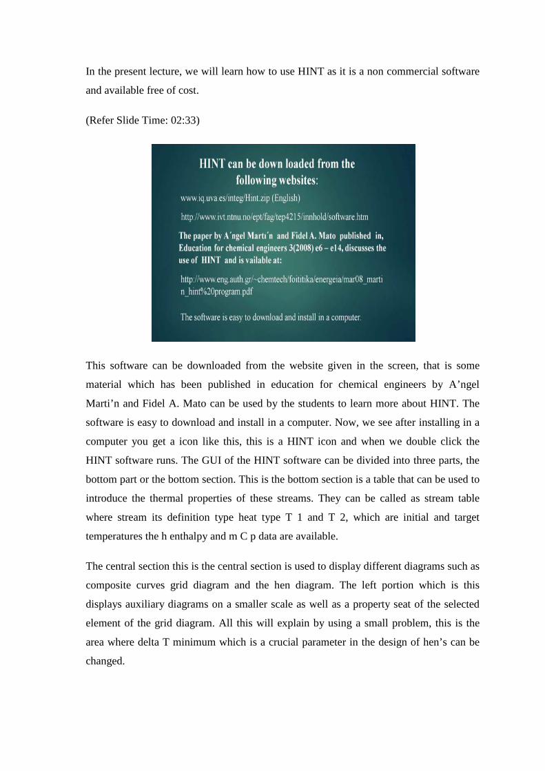
In the present lecture, we will learn how to use HINT as it is a non commercial software

and available free of cost.


This software can be downloaded from the website given in the screen, that is some

material which has been published in education for chemical engineers by A’ngel

Marti’n and Fidel A. Mato can be used by the students to learn more about HINT. The

software is easy to download and install in a computer. Now, we see after installing in a

computer you get a icon like this, this is a HINT icon and when we double click the

HINT software runs. The GUI of the HINT software can be divided into three parts, the

bottom part or the bottom section. This is the bottom section is a table that can be used to

introduce the thermal properties of these streams. They can be called as stream table

where stream its definition type heat type T 1 and T 2, which are initial and target

temperatures the h enthalpy and m C p data are available.

The central section this is the central section is used to display different diagrams such as

composite curves grid diagram and the hen diagram. The left portion which is this

displays auxiliary diagrams on a smaller scale as well as a property seat of the selected

element of the grid diagram. All this will explain by using a small problem, this is the

area where delta T minimum which is a crucial parameter in the design of hen’s can be

changed.

Now, let take a small problem and demonstrate it, so to start with we go to the streams

and then we go to add. Now, it opens up a window to enter the stream data the stream

data can be of two types, one is non linear type another is linear type this is a linear

stream data where m C p is constant. This shows a non linear stream data, where m C p

changes with temperature. Now, we start with the non linear stream data which is

seldomly used in demonstration purposes, but we start with this. So, we click the radio

button of non stream non linear stream data and then we go to the enthalpy, it opens up a

table like this. In this table we can fill a non linear stream data which comprises of

temperature and enthalpy.


Now, we take a small problem for filling the non-linear-stream data, here you see the

temperature and enthalpy 180, the enthalpy is 0, 160 enthalpy is minus 800 and so on so

forth. In the last, temperature is 70 where enthalpy is minus 2400. This is a data for a hot

stream, where the temperature is changing from a higher temperature to a lower

temperature. This stream is giving heat to the system and that is why the enthalpies are

negative.

So, we again come to this table to fill this data, so I will filled then I press add this

temperature is 140 the enthalpy is minus 1200. Then again I press data this temperature

is 120 and this enthalpy is minus 1600, then again I press data this enthalpy is 100, this

temperature is 100 and the enthalpy is minus 2,000. Again, I press data this temperature

is 800, enthalpy is minus 2200, the last temperature is 700 and the enthalpy is minus

2400.

So, once I fill this data this is the enthalpy temperature diagram which is visible here and

this can be used in the computation of hen, so we cancel this. Now, we go for linear

stream data’s, so I again open the stream data table. Let us take a small problem, where

there are two hot streams and two cold streams.


This is shown in table one four stream problem for load integration and utility

predictions; this is the table where there are two hot streams and two cold streams. The

supply temperature of the first hot stream is from 180 to 75, it is C P which is basically

m C p is 30. The second hot streams moves from 240 to 60, the C P is 40, the first cold

stream C 1 is 40 to 230 degree, the CP is 35, the second cold stream is 120 to 300 the CP

is 20. So, we are going to feed this data and see how the program deals with it.

Now, this is stream number one the description is H 1, now the supply temperature is

180 and the target temperature is 75. I want to introduce the m C p data, so I click this

radio button and enter the m C p data as 30 given in the problem while inserting data. It

can be inserted in two mode m C p mode and delta H mode. So, if I try to introduce delta

H, I can on this radio button and introduce my delta H which is 3150 in this case, but

however we will for this problem. We will introduce the m C p data and not delta H data

which is 30.

Then, I go to the next stream, I press the add button this number changes to 2 and the

second stream is H 2. The supply temperature is 240, the target temperature is 60 and the

m C p value is 40, so I go to the next stream. Now, I put add this is C 1 the first cold

stream its supply temperature is 40 and its target temperature is 230 and the m C p value

is 35. I again press add this goes to the forth stream the stream number is C 2, its supply

temperature is 120 and its target temperature is 300. Now, completed my problem and I

can press.


Now, whatever data I have feed it has come to here all the stream data you can match

this is H 100, this is hot stream, the heat type is sensible. The supply temperature is 180

and the target temperature is 75 heat exchange is 3150 kilowatt and the m C p value is

30, so the complete stream table has come to this. Now, this shows the great diagram and

here we see the composite curve a small composite curve and this show about the

streams. So, this shows the first stream H 1 and the supply temperature 180, target

temperature 75, I can press this, so I to see the data stream 2. I can press this stream 2, if

I want to see the data stream 3, I can press the stream 3, it comes to the cold one if I want

stream 4, I can press this.

So, in short we can also see the complete data from here also or we can also see from

here. Now, after we have feed the data then we can this menus are available for further

processing, I can see different diagram by pressing the diagram menu, if I want to see a

composite curve.


I can press this, I get the composite curve, it is in a small, and it is a big composite curve.

I can reformate it or going to the format statement, I can change this width and height

say suppose, I make it 20, I make it 20. I can change the fonts of the axis scale legend

axis titles etcetera, I can write down the x axis title, y axis title. Other things can be

change from here, so when I press this enlarges this enlarges the composite curve.

Now, I take a second problem of data feeding and that is given here, the second problem

it is a four stream problem where two hot streams and two cold streams. H 1 changes

from 150 degree centigrade to 50 degree centigrade C P is 2 and delta H is minus 80. Let

us feed this and see what happens, so I go here it shows me the last problem. So, I have

to press here new and then I press stream and add. So, in this case H 1 and the supply

temperature is 140 the target temperature is 50 and the value of m C p is 2 then I add it

changes to 2, so the second stream is H 2.

The supply temperature is 90 this target temperature is 40 and the value of m C p is 6, a

third stream is C 1 cold one and the supply temperature is 30. Target temperature is 150

and the value of m C p is 2, we go to the forth stream this is C 2, the supply temperature

is 70. The target temperature is 125 and the m C p value is 3, once all data related to the

stream temporal has been entered with and press. So, the stream temporal appears here

and the grid diagram appears here in the grid diagram. You see that this line corresponds

to pinch line the hot pinch is 90 degree the cold pinch is 80 degree, the first stream

moves from 140 to 50.

The enthalpy exchange is minus 180, the minus sign shows that it is a hot stream the m C

p value is 2 shown here, the second stream starts from the pinch itself. It is a hot stream

moves from 90 degree to 40 degrees centigrade, it exchanges an enthalpy minus 300 and

its value is 6 the first cold stream, it is C 1 the stream number is 3 moves from 30 degree

to 150 degree. It exchanges 240 units of heat that means, it requires 240 units of heat to

be heated from 30 to 150 its m C p value is 2.

This is the fourth stream which is second cold stream starts from 70 degree goes to 125

degree exchange is 165 units of heat and its m C p value is 3. Now, this shows how to

feed the data using this computer using this computer program which is HINT. Now, we

will go for a small problem and we will show you how to do energy targets and unit

target calculations using this HINT now for this.


We take up this problem, this is table 2 problem here also there are two hot streams and

two cold streams. Using this we will show you the energy target and unit target

calculations using HINT. Now, we start with a new problem here, so we go to the stream

go to this add. Now, here you will see that in this problem the delta T minimum is 10 and

here this delta T minimum is 10, so we do not have to change it. If you will have a

different value, you can change the delta T minimum from here.

Now, we enter the data this is H 1 140 and this is 50, m C p value is 2, add second stream

H 2 supply temperature is 90. Target temperature is 40, m C p value is 6 add this third

stream this is C 1 30 supply temperature target temperature is 150 and m C p is 2 and

forth stream this is C 2. Supply temperature is 70 and target temperature is 125 and m C

p value is 3, so we press here the stream temporal appears here we can check this appears

to be ok. Now, this is our hot composite curve and this is our cold composite curve.


So, if I see the composite curves this is my hot composite curve and this is my cold

composite curve, now I revert back to my grid diagram here. Now, you see if I press this

then this stream in this composite curve starts from here to here. It becomes green, so

this is available from here to here and if I press this, it is available from here to here.

Now, if I press this it appears into the cold composite curves are goes from here to here

and the second this is from here to here and some part from here to here. So, what do I

mean that when you press a stream, its contribution in the cold as well as hot composite

curves is visible in this small diagram.

So, this again we go to the composite curve if I want to enlarge it a little, so I can go here

I can add this to say S 120 and to this make this 20 and it enlarges. So, this is my hot

composite curve and this is my cold composite curve the relative position of these two

curves depends upon this delta T minimum. Delta T minimum is the distance from here

to here the vertical distance where the two curves are closes to each other. Now, from

this the hot stream can give heat to this cold stream, but from here onwards there is no

stream available to give heat to this cold stream.

So, this has to be given by a utility and here also if I draw a vertical line from here to

here, the hot stream from here to here are able to give heat to the cold stream, from here

onwards there is no cold stream which will take heat from this hot stream. Hence, this

has to be taken by a cold utility. Now, if I go for energy target I can press this it gives me

a cascade diagram which is called P T A. I get the P T A, here it shows minimum

temperature difference 10, heat duties 175 that is q h minimum is 175 kilowatt and

cooling duties which is q c minimum is 250 kilowatt, and the pinch temperature is 85.

So, to get hot pinch temperature I have to add to this delta T minimum by 2 and to get

the cold pinch temperature, I have to deduct from this data that is 85 cold delta T

minimum divided by 2, which is available in the stream diagram. Now, this energy target

which is shown here is dependent on this minimum temperature difference. So, if I

change minimum temperature difference here say make it 20 and press then what I find

that this value changes, now this is 225 and 300. I can change it further to 30 degree

centigrade, this again changes to 45 to 320 again I can change it 240 degree centigrade,

again this changes I can make it to 50 degree centigrade it further changes.

So, what we observed that we if we change delta T minimum the energy target changes,

now this shows the minimum number of heat exchangers, this is unit’s target. Now, if I

change delta T minimum this unit targets also changes, if I make it 10 then I find that my

units target is 7. So, from this table I can find out the energy target as well as units target.

Now, if I want to get a complete picture of this then I can go to a different menu, this is

streams this is cascade diagram. Just a minute, so I can go to the delta T minimum

analysis I can go to the here, so I can fix up this minimum temperature differences 10 to

5 number of points 50 and I say ok.


It shows how the hot utility and the cold utility are changing when delta T is minimum, I

can go to this, further I can ask that how the pinch temperature is changing.


This pinch temperature is changing like this when the delta T minimum is changing from

say 1 degree centigrade to 50 degree centigrade. I can also see that how my minimum

number of heat exchangers is changing when the delta T minimum is changing from 1 to

50.


So, we see around 20 degree value of delta T minimum there is sudden change below

this the number of units required is 7 and after this the number of units required is 6, it is

minimum. It is minimum number of units required for the heat exchanger, so we see the

effects here. Now, if I want to change, we again go to the stream grid diagram, if I want

to change the m C p of a certain stream, it also affects the grid diagram. Let us see it, let

me change it to 10 and then I say enter not changed.


Now, it has changed, now you see that once this changes to 10 in place of 2, the whole

grid diagram changes the value of the pinch which was earlier 19 and 80 changes the

placement of streams also changes. So, I go back to two and you observe the change,

now you see this has completely changed. So, we conclude that the m C p value or the

stream affects the grid diagram and also the composite curves, the delta T minimum

value affects the utilities that is q h minimum and q c minimum values and units target.

So, by these examples now we are able to understand how the energy targets and unit

targets are computed, and what are the different parameters, which affect the energy and

unit target. We will take the same problem that is table number 2 to demonstrate other

features of this software HINT. Now, if we go to the diagram menu then you have

different diagrams are available composite curves, composite curves with utilities grand

composite curve, available temperature difference grid diagram energy, composite

curves energy grand, composite curves available energy etcetera.

So, we are not going to use this energy composite curve and energy grand composite

curve and available energy, but we will use all these above diagram that is composite

curve. Composite curves utilities, grand composite curves available temperature

difference grid diagram delta T minimum analysis, I have already shown you loops and

paths. So, the next diagram is our grand composite curve, so if I press grand composite

curve, I see a grand composite curve here.


So, you can directly draw your grand composite curve using the software and you can

take a print out from here using the print menu. Now, if I go to the second that is

available temperature difference.


It shows me the available temperature difference, it is drawn between A T cold and T

hot. We will discuss a lot about this when we will go for the remaining problem analysis

and driving force plot in the grand composite curve from here to here. It shows the hot

utility requirement and from here to here, it shows the cold utility requirement, you all

know about the grand composite curves. So, if you want to draw you can use this

software then if you go to these streams, you can add stream using stream command, you

can delete a stream, you can split a stream.

You can find out the cascade, this is the cascade and then you can use the feasibility, this

feasibility menu is used for the design of heat exchangers. It has got two parts above

pinch and below pinch an above pinch and below pinch rules can be used to design a

heat exchanger network, this gives you the area target and this gives you the cost target.

Now, in the heat exchanger menu’s, you can add a heat exchanger, you can delete a heat

exchanger, you can go for the area and cost calculations. It shows the results in which it

gives you the details of all the heat exchangers available in the heat exchanger network.

This can be used for remaining problem analysis which gives correct direction to a heat

exchanger design, when we are using our own utilities that means user defined utilities.

Now, if you see this HINT program, HINT program uses the utility in two ways if you

do not give cold and hot utilities the HINT program itself assumes cold and hot utility

depending upon the stream data. It also gives you a facility to define your hot and cold

utilities and with this add menu, you can add a cold and hot utility. The delete menu

deletes cold and hot utility, combine menu it combines the hot utility and the cold utility

with the stream data. So, this is the stream data and when you use this combine it

combines the hot utility and cold utility. You must have seen that for targeting, we can

combine the hot and cold utility with the steam data.

We can go for the area targeting, it also gives you the cost data in the loops and path are

used for identification of loops and heat transfer paths in a heat exchanger network, when

we go for the design of a heat exchanger network. The first design is a M E R design,

maximum energy recovery design and then maximum energy recovery design is further

modified to get a low cost heat exchanger design by avoiding, or by you can say the

pinch is violated in that to save the number of units. When we will talk about the design,

we will see that the M E R design can be modified, or improved upon by breaking the

loops.

So, here in the loops and paths dropdown menu, you get all those facilities which are

used to break the loops and to detect the temperature paths, or enthalpy paths through

which the heat can be transferred from hot utility to the cold utility. This gives you the

diagrams this gives you the tools different tools. So, in a nutshell we have seen that what

this program can do and these are the small icons through, which this is icon where

through which I can go to the composite curve. This is icon where I can go to the grand

composite curve.

This is icon where I can go for the delta T minimization for that I have give the cost data

that is why it is fronting me to give cost data this gives you the grid diagram. So, icons

are basically used when we do not want to use these dropdown menus. Now, we take a

problem new problem which will show us the area target, we know that there are

different targeting schemes in which energy target is a units target and then area target.

So, we will now take a problem and demonstrate the area target.


So, this is the problem which is given in table three a five stream problem for cost

targeting and area targeting basically for the cost target. We will have some more data

which are required in the area target, you will see in this table that for area targeting. We

need the stream data plus the heat transfer coefficient data for all the streams here we can

add the utilities. Here, there are two utilities, one is stream and the other is cooling water

steam is transferring heat through latent heat and cooling water is transferring heat

through sensible heat.

The supply temperature here is 300 and 299 and for cooling water it is 20, supply

temperature and target temperature is 60, here we will see that the temperature is taken

for the stream is 300, 299. We know that the stream heating is a constant temperature

heating, it should be taken 300 and 300 instead of 300 and 299. We should take 300, but

if I take 300 then my computation of C P will be infinite, further if you see a practical

problem when a cold stream is heated by stream. There is a pressure drop from the

location where stream is injected to a location where a stream drawn out.

So, due to this pressure drop the temperature drop will also occur and if I am taking this

temperature to be 300 and 299, I am not committing any mistake because this is in heat

balance and in the computations no error will be introduce. Now, let us start the area

targeting using table 3 data, so start introducing the data. So, this is stream data I had this

is H 1 159, 59, 77 the value of m C p is 22.85, the second is H 2 the supply temperature

is 267 and target temperature is 80 and this is 2.04.

The third is H 3, there are three hot streams supply temperature is 343 and target

temperature is 90 and m C p value is 5.385, 0.38. The forth is C 1 the supply temperature

is 26, the target temperature is 127, m C p value is 9.33. The last one fifth stream which

is a cold stream, it is called C 2 supply temperature is 180 and target temperature is 265

and m C p, sorry target temperature 265 here and m C p values is 19.61. Now, we have

fed our stream data, but we have not fed the stream heat transfer coefficient.

Now, this can be handle in a two way in the first case we will not feed our cold and hot

utilities as given in the table stream table. So, we have already fed the stream data you

set, now we have gone to the stream data and area target. Now, in this using this tabular

format, we will feed the heat transfer coefficients half different streams if I see this, it

has been written stream one. Heat transfer coefficient is 2 kilowatt per meter square

Kelvin, so default data of heat transfer in hint is 2 kilowatt per meter square and Kelvin.

So, here stream number one 2 kilowatt, if I change this stream to two still it is 2 kilowatt,

to three 2 kilowatt, to four 2 kilowatt, to five 2 kilowatt to six 2 kilowatt for five because

we have five streams.

Now, utility we see the utility number one which is heating hot utility its heat transfer

coefficient has also been taken to and the temperature has been taken 348. If I go to the

cold stream again the heat transfer coefficient is 2 and the temperature of the cold one.

So, there are the default values of heat transfer coefficient in the HINT, but we can

change this like in our problem the heat transfer coefficient of stream one is 0.1, so I

write is 1. So, there is a problem in this software, you have to keep this decimal value

intact if you delete this that is a problem in entering, so 0.1 then I go to two then I delete

this two, but I keep the decimal value then I put it here 0.4.

Then I go to the stream number three and the heat transfer value is 0.5, stream number

four the heat transfer value is 0.01 and for the fifth stream this is 0.5. I am not entering

the heat transfer values of the utilities here this steam is 0.05 and the cooling water is 0.2

I am not entering this values and do not consider this values. The heat transfer coefficient

values are very accurate because in the problem we have taken some representative

values for showing you the calculation.

Now, if I do this it clearly shows the area target is 3523.29 meter square the number of

minimum heat exchange that is unit target is 8. So, directly I get a value here, now what I

can do, so if I go again go to the area target I see the value is 3643.33. The earlier value

is wrong because it has not executed, now it has a executed completely this software.

Hence, the area target when not feeding the hot and cold utilities and computer is taking

default values of hot and cold utilities, the area target obvious to be 3643.33 meter

square.

Now, let us try to give the values of the heat transfer coefficient of utilities, so the first

utility is heating. So, here the coefficient is 0, 5 and the second utility this coefficient is

0.2, so this is 0.2, so if I say ok. So, it changes the value of area target changes, now we

must be wondering that how to field the temperature levels of the cold and hot utilities.

So, let us see how to do it, now you see here the minimum temperature difference is 10 if

I make it 20 my area target will also change, you see these are change. So, by changing

the temperatures you can also see that the area target changes.


Now, if you go to the here that is a utility, now I can do it plus this is cooling utility say I

am pressing on the latent heat. The supply temperature is 300 in our case and target

temperature is 299. So, I say this, so it exchanges a heat up minus 1,295 and it makes it

sensible because here the temperature is changing from 300 to 299. Basically, I have

approximated the latent heat transfer to a sensibly transfer and say I say plus it is cooling.

It is not a latent, so I have to make it sensible and then this temperature is 20 and this

temperature is 60. So, I say this adds say the clue.


Now, I can go to the combine to add this to utilities so if I draw this when it goes here

the value is added up heating values and the cooling 300 degree, let me check. There is

stream which is 343, so we have to increase the temperature of the hot utility then only it

up here, so let us change. So, make it 400 degree say 360 will also do and this 359. So,

my this line shows my hot utilities which is above the harsh temperature of the grant

composite curve the cold utility, the lowest temperature is may be 26, so cold utility 22,

60 may work.

So, this shows you the cold utility line and this shows you the hot utility line, so I can

combine them. Let us go to the area target again and I see the area target now changed.

So, this result which I get is when I am utilizing user defined hot utility and cold utilities,

so I get area target which is this. Now, I can also see that the how the area target changes

with delta T minimum, so if do this I get curve like this.


So, when delta T minimum is increasing the value of the area target that means area

which is required for the total heat exchanger is defining. This shows that when delta T

minimum increases the fixed cost of the heat exchanger network decreases.

Thank you.

process integration prof. bikash mohanty department of...

Documents