processes

Article

Optimal Design of a Carbon Dioxide SeparationProcess with Market Uncertainty and Waste Reduction

Juan Pablo Gutierrez 1,*, Eleonora Erdmann 1 and Davide Manca 2

1 Instituto de Investigaciones para la Industria Química (INIQUI, CONICET-UNSa), Facultad de Ingeniería,Universidad Nacional de Salta. Av. Bolivia 5150, Salta 4400, Argentina; eleonora@unsa.edu.ar

2 PSE-Lab, CMIC Department, Politecnico di Milano, P.zza Leonardo da Vinci 32, 20133 Milan, Italy;davide.manca@polimi.it

* Correspondence: gutierrezjp@unsa.edu.ar

Received: 11 March 2019; Accepted: 27 May 2019; Published: 5 June 2019�����������������

Abstract: The aim of this work is to optimize the conceptual design of an amine-based carbondioxide (CO2) separation process for Enhanced Oil Recovery (EOR). A systematic approach isapplied to predict the economic profitability of the system while reducing the environmental impacts.Firstly, we model the process with UniSim and determine the governing degrees of freedom (DoF)through a sensitivity analysis. Then, we proceed with the formulation of the economic problem,where the employment of econometric models allows us to predict the highest dynamic economicpotential (DEP). In the second part, we apply the Waste Reduction (WAR) algorithm to quantify theenvironmental risks of the studied process. This method is based on the minimization of the potentialenvironmental indicator (PEI) by using the generalization of the Waste Reduction algorithm. Resultsshow that the CO2 separation plant is promising in terms of economic revenues. However, the PEIvalue indicates that the higher the profitability, the larger the environmental risk. The optimal valueof the DEP corresponds to 0.0274 kmol/h and 60 ◦C, with a plant capacity according to the mole flowrate of the produced acid gas. In addition, the highest environmental risk is observed at the upperbounds of the DoF.

Keywords: optimal conceptual design; market prediction; economic uncertainty; environmentalimpact; carbon dioxide separation

1. Introduction

Several stages exist to recover the original pressure of mature oil and gas wells. Among thosealready applied, the Enhanced Oil Recovery (EOR) with carbon dioxide (CO2) proved to be a mid-termsolution to increase the oil production to its original levels while capturing thousands of tonnes ofCO2 [1,2].

Haszeldine [3] states that the first injections of carbon dioxide into the microscopic pores ofsedimentary rocks date from the early 1970s. Successful cases of CO2-EOR have been reported inthe United States, United Kingdom, Norway, and Canada by Wright et al. [4] and Mumford et al. [5].The injection of CO2 was also evaluated in the reservoirs of Argentina, a region where EOR pilotexperiences were barely intended. Although the results provided good revenues, the CO2-EOR in theregion remains unmaterialized after more than twenty years since first being discussed [6].

The main problem related to this procedure is the large and continuous amount of CO2 necessaryto start the EOR injection [7]. In this regard, Herzog [8] reports that the common sources for largeamounts of CO2 correspond to the acid gas coming from natural gas processing.

Kwak et al. [9] compare different technologies for CO2 separation from natural gas. Based onsimulation and economic studies, they conclude that chemical absorption with methyldiethanolamine

Processes 2019, 7, 342; doi:10.3390/pr7060342 www.mdpi.com/journal/processes

Processes 2019, 7, 342 2 of 17

(MDEA) is the least expensive and most feasible option to separate carbon dioxide. Moreover,Leung et al. [10] note the amine processes’ high efficiency, large amounts of acid gas as a side product,and the possibility to regenerate the solvent. Other comparable processes include separation withpolymeric membranes, cryogenic separation, physical solvents, and hybrid technologies.

Another task when evaluating CO2-EOR possibilities is the large dependence of oil and gascompanies upon economic conditions and countries’ institutional frameworks [11]. For instance,Ponzo et al. [12] state that changing market structures influence the long-term evolution of gasquotations and, consequently, the development of gas fields. Moreover, interdependency amongvariations of time with technical, operative, and economic conditions has been assigned to performeconomic evaluation by Manolas et al. [13]. Classically, the interaction between the operating aspectsand economic revenues during the definition of a process is first estimated according to the conventionalconceptual design [14]. Conceptual process design (CD) consists of the selection of proper operationunits, their sequences, and the recycling structure needed to obtain a specified product [15]. However,Sepiacci et al. [16] explain that this conventional method is no longer representative when consideringmarket uncertainty, demand and offer fluctuations, and the price instability of commodities and utilities.Then, Manca and Grana [17] introduced the benefits of dynamic conceptual design (DCD). Based onCD and the economic potentials (EP) presented by [14], DCD takes into account the dynamic featuresof price/cost fluctuations within a given time horizon.

Indeed, the process design of chemical industries are considered complete when performing theenvironmental risk analysis of new process systems. Currently, there is a great deal of interest inthe development of methods that can be used to minimize the generation of pollution, and there arenumerous efforts underway in this area [18]. Specifically, this interest has increased with the world’sawareness of CO2 emissions and made process engineering adopt practices to mitigate the effects ofclimate change [19].

For the above reasons, we apply the concept of DCD to obtain and condition CO2 for EORpurposes. As can be anticipated, we focus our study to establish the conceptual design of the processin the context of market instability and future uncertainties. CO2 for EOR is obtained from a naturalgas sweetening design that uses MDEA as solvent; the specifications for the produced CO2 include a95 mol% concentration of the acid gas, compressed at 6500 kPa [20].

An optimization problem is formulated with the aim of minimizing the Dynamic EconomicPotential (DEP) of the design. In this sense, Mores et al. [21] state that two degrees of freedom (DoF)govern the optimization problem of the CO2 MDEA absorption—the recycled amine flow rate and itstemperature. However, we extend the analysis to prove that the variable most affecting the energydemands of the plant is the water makeup of the amine solution, and thus more proper DoF.

Then, we analyze the historical prices of products and raw materials by using statistical tools.We present natural gas prices as references to estimate the evolution of the rest of the involvedcomponents by using numerical correlations. Linear Regression Models (such as AutoRegressivemodel with an eXternal input, ARX) are applied to interpret the behavior of past quotations. We switchthe contribution of these economic models into econometrics to make them capable of predictingquotations and generating future market scenarios.

On the other hand, we perform an assessment to find the pair of DoF that reduce the environmentalpotential index. The method is adapted from the Waste-Reduction algorithm applied to chemicalprocesses presented by Young et al. [22]. The Waste Reduction (WAR) algorithm has been developedto describe the flow and the generation of potential environmental impact through a chemical process.

2. Process Description

The purpose of a natural gas sweetening process is to remove the acid gases from a sour naturalgas stream. Due to the high selectivity of the solvent, the by-product of this process is a high-purityCO2 material stream that, after conditioning, can be used as an EOR fluid.

Processes 2019, 7, 342 3 of 17

The regular process of natural gas sweetening to obtain CO2 is divided into two parts [23]. In thefirst stage, which consists of an absorber column, the natural acid is put in countercurrent contactwith a descending MDEA aqueous solution—a so-called lean amine [24]. Fouad and Berrouk [25] andKazemi et al. [26] indicate that low temperatures and high pressures favor the exothermic reaction thatoccurs in the unit. After contact, the aqueous solution of amine is pressurized, heated, and sent tothe regeneration stage [27]. This second stage consists of a distillation column where the acid gas isremoved from the amine solution due to an external heat contribution. Different studies have beenperformed in order to optimize the energy requirements of the regeneration column [28–30]. The liquidfrom the regenerator column is cooled and pumped back to the absorption stage [31,32]. Water andMDEA are placed in the stream from the bottom of the column to the absorption tower to compensatefor leaks within the operation. Meanwhile, the high-purity CO2 from the top of the regenerator issent to a series of four centrifugal compressors to considerably increase the pressure. Original wellpressures are required to dispose of the CO2 as an injection fluid; in this case the value remains over6500 kPa. The 4-stage compression design includes intercooling units and intermediate separationstages [33].

3. Methods

3.1. Simulation Base Case

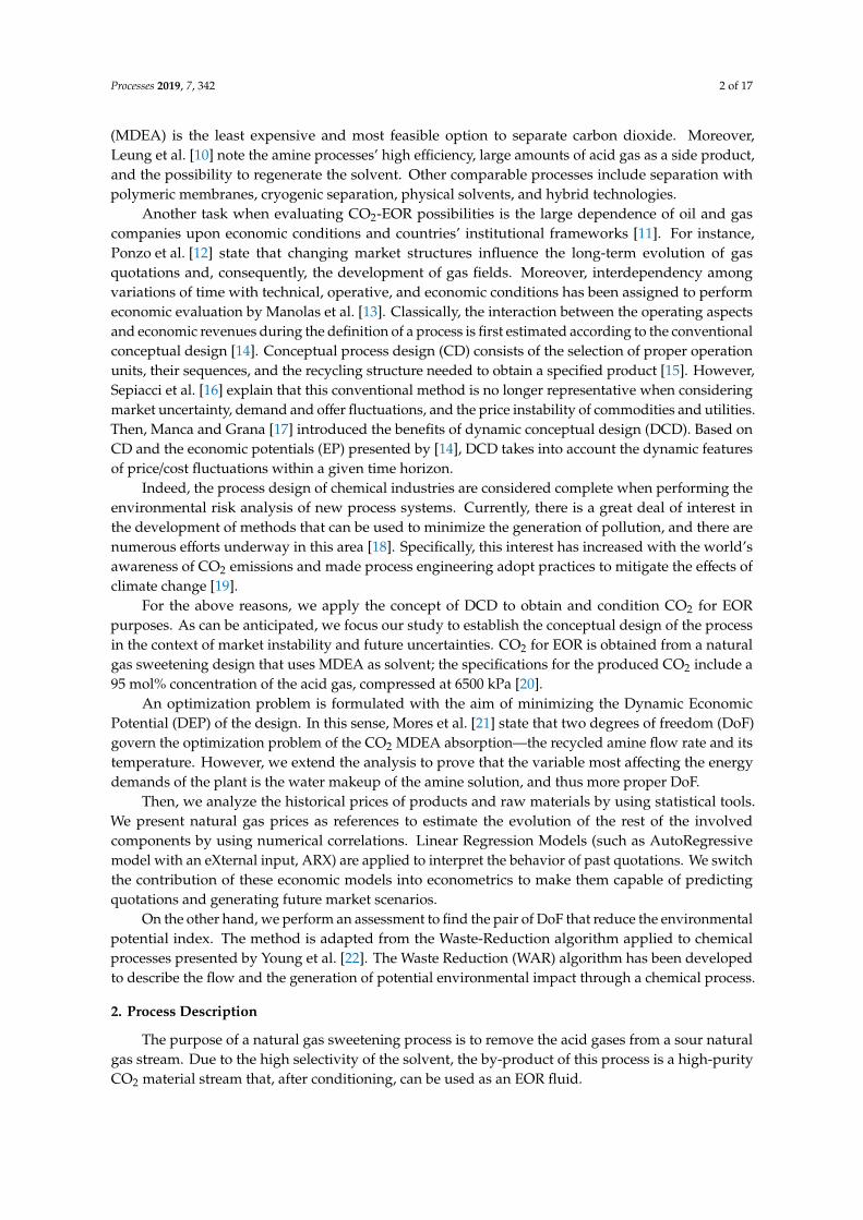
A process of CO2 absorption and compression is modeled by using UniSim [34]. Natural gasat a value of 2500 mm3/d is assumed as the plant’s capacity. The conditions of the plant are thosereported in the work of Gutierrez et al. [19]: sour natural gas at 35 ◦C and 6178 kPa with 93 and 4 mol%of CH4 and CO2, respectively. Also, the conditions of the lean amine are reproduced. We consider21,000 kmol/h of an aqueous MDEA solution (38 wt%), at 42 ◦C and 9610 kPa. A 24-tray absorptioncolumn operates at the pressure of the inlet gas. Rich MDEA from the bottom of the absorber is flashedat 441 kPa, heated up to 90 ◦C, and then sent to regeneration. The regeneration column consists of24 trays and operates at 90 ◦C and 443 kPa. To provide the column with an external heat, we assume areboiler unit using natural gas as fuel. Recycled MDEA is pumped and cooled, first exchanging heatwith the rich amine, and then with a cooler so that it reproduces the temperature of absorption.

A 4-stage compression system is employed to increase the pressure of the produced CO2 up to6865 kPa [33]. Figure 1 shows the simulation of (a) the CO2 separation plant and (b) the compressionsector to produce the high-purity CO2 stream.

Muhammad and GadelHak [35] explain that the main variables affecting CO2 absorption aresolvent flow rate and the absorber temperature, this last through the cooling of the lean amine stream.

As we anticipated, two streams conform the solvent inlet flow stream, one corresponding to a pureMDEA stream and the other connected to the makeup water. Generally speaking, two independentvariables are related to the same degree of freedom, so in this study we determine whether there is astrong dependency between the main energy requirements and the independent variables. Similar toTorres-Ortega et al. [36], we perform a sensitivity analysis to evaluate suitable ranges of variation forthe decision variables along the optimization.

3.2. Predictive Concept Design

This section provides the dynamic approach to the economic assessment for the CO2 conditioningplant. Econometrics models (EM) are employed to simulate and evaluate future trajectories of pricesand costs.

Processes 2019, 7, 342 4 of 17

Processes 2019, 7, x FOR PEER REVIEW 4 of 17

(a)

(b)

Figure 1. Simulation model in UniSim: (a) absorption sector and (b) compression sector. Figure 1. Simulation model in UniSim: (a) absorption sector and (b) compression sector.

Processes 2019, 7, 342 5 of 17

3.2.1. Development of Econometric Models

The first step while performing EM is the selection of a reference component (RC). Manca [37]employs RC historical quotations to estimate the economic dynamics of all commodities and utilitiesin the process he analyzed. Moreover, Manca [38] suggests that an RC must be representative of thesector where the plant operates, with the availability of frequent data and updated price evolution.

A good RC for the industry of Oil and Gas is crude oil (CO) [39]. CO, and also the evolution ofnatural gas (NG), quotations are traced daily for EIA [40]. However, the prices of natural gas producedin the basins of Argentina are also indicated monthly by the Ministry of Energy [41]. In this study,we perform the EM for both CO and NG as potential candidates for reference components.

A structural auto regression model is applied to separately autocorrelate both West TexasIntermediate (WTI) crude oil and US natural gas prices [42]. For both potential candidates, we analyzemonthly quotations from July, 2007 to July, 2017 (the last available date). To correlate the historicalvalues of the quotations, we use a similar methodology as the one used by Zhou et al. [43] regardingthe coefficients of the Pearson equation (Equation (1)). Pearson coefficients (PCs) measure the strengthand direction of the linear relationship between two random variables [44]. In this case, both variablesrepresent the monthly quotations of the RC, but differ in one period:

rk =

∑t=k+1

(Yt −Y

)(Yt−k −Y

)∑n

t=1

(Yt −Y

)2 (1)

where rk denotes the PC for a particular period.∑

t=k+1

(Yt −Y

)(Yt−k −Y

)is the covariance of the

quotations (Yt) with respect to one-period of the previous quotations (Yt−k), and∑n

t=1

(Yt −Y

)2is the

squared of the standard deviation. rk varies from –1 to 1 and, in general, the higher the correlationcoefficient, the stronger the relationship is [45]. Dancey and Reidy [46] state that if rk ranges from 0.7 to0.9, the strength of correlation is high, and quite enough to determine the size of the correlation. Thischaracteristic can be visualized when plotting the coefficient versus the time lag between the quotations.

3.2.2. Formulation of the Economic Optimization

Once the EM are identified, it is viable to run the grid-search optimization according to theregular process conceptual design (PCD). In the optimization problem, we determine the set ofDoF that maximizes the cumulated value of the Dynamic Economic Potential of order four (DEP4),Equations (2)–(4).

(Cumulated)i =N∑

j=1

DEP4 j,i; i = 1, . . . , I (2)

DEP4i

(USD

y

)=

N∑j=1

Revenues j,i·nHpY −CAPEXN/12

(3)

Revenues j,i

(USD

y

)=

NP∑p=1

Cp, j,i·FP −

NR∑r=1

Cr, j,i·Fr −OPEX j,i (4)

where DEP4 is the fourth-level economic potential calculated for the i− th economic scenario. j, i arethe subscripts for a specific month and scenario, respectively; nHpY is the number of working hoursper year. N stands for the number of months to perform the economic assessment. NP, NR, FP, and Fr

represent the number of products and reactants, their flow rates, and C their costs. The CAPEX term isestimated according to the empirical equations reported by Douglas [14]. Six main units are consideredfor the calculation: absorber and distillation columns, MDEA heat exchanger, and two air coolers.

The OPEX term considers a price trajectory for each raw material, by-product, and utility, for thei− th scenario. The main contributors of the OPEX are two air coolers, a condenser, reboiler fuel, and

Processes 2019, 7, 342 6 of 17

the total power required for the acid gas compressors (Gutierrez et al. [19]). The material and energybalances required to calculate the OPEX are taken from the steady-state simulation of the process.

The goal of the optimization is to determine the combination of DoF that maximizes the value of(Cumulated)i, with respect to a set of generated scenarios, where the assessment becomes probabilistic.To obtain a high-purity CO2 material stream, Gutierrez et al. [19] use a limit value of 2 mol% in the gascoming from the top of the absorber, so we consider the molar fraction of CO2 as a restriction for thestated problem.

3.3. Waste Reduction Algorithm

We employ the Waste Reduction (WAR) algorithm to describe the flow and the generation potentialenvironmental impact through the process under study [22]. The general methodology of the WARalgorithm defines Potential Environmental Impact (PEI) indexes to characterize the generation of thepotential impact in a process, divided into eight categories.

The first four categories evaluate, globally, the environmental friendliness of a process: humantoxicity potential by ingestion (HTPI), human toxicity potential by exposure (both dermal and inhalation)(HTPE), terrestrial toxicity potential (TTP), and aquatic toxicity potential (ATP).

On the other hand, the other four are related to the toxicological aspects of the involved chemicalswithin the process: global warming potential (GWP), ozone depletion potential (ODP), photochemicaloxidation potential (PCOP), and acidification potential (AP).

The potential environmental impacts are calculated from stream mass flow rates, streamcomposition, and a relative potential environmental impact score for each chemical present inthe separation process [18].

According to the notation of Young and Cabezas [47], the output PEI to the chemical process canbe rewritten as Equation (5):

i(cp)out =

N∑w=1

.M

(out)w

∑i

xi,wψi (5)

ψk =∑

l

αlψsi,l (6)

where.

M(out)w is the output mass flow rate of stream w, xi,w is the mass fraction of the chemical i in

the stream is w, and ψi is the overall PEI for the chemical k. ψi can be calculated from Equation (6).In Equation (6), ψs

i,l is the normalized specific PEI of chemical k for the impact category l, and αl is therelative weighing factor of impact category l [39,47]. A unitary value is assigned to α, to illustrate thecase where the eight categories have the same importance in our evaluation [48]. Normalized impactscores are obtained from the WAR algorithm add-in included in the latest release of the CAPE-OPENto CAPE-OPEN (COCO) Simulation Environment, available from http://www.cocosimulator.org/ [49].

4. Results

4.1. Simulation Output

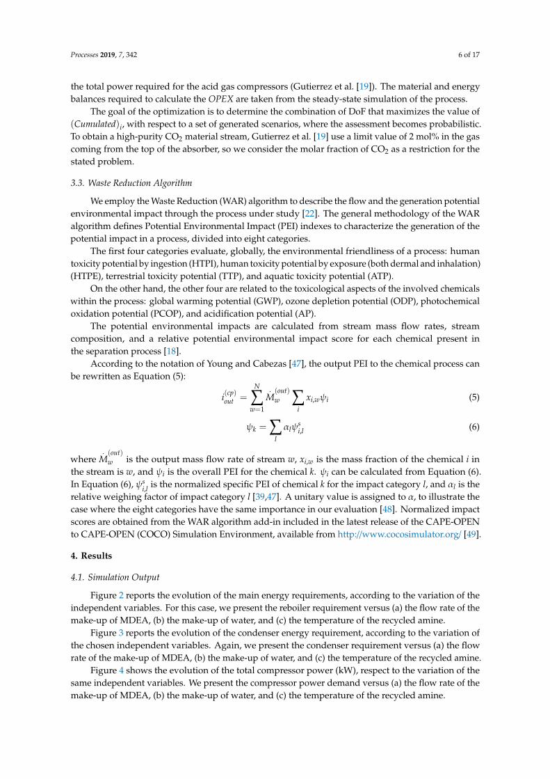
Figure 2 reports the evolution of the main energy requirements, according to the variation of theindependent variables. For this case, we present the reboiler requirement versus (a) the flow rate of themake-up of MDEA, (b) the make-up of water, and (c) the temperature of the recycled amine.

Figure 3 reports the evolution of the condenser energy requirement, according to the variation ofthe chosen independent variables. Again, we present the condenser requirement versus (a) the flowrate of the make-up of MDEA, (b) the make-up of water, and (c) the temperature of the recycled amine.

Figure 4 shows the evolution of the total compressor power (kW), respect to the variation of thesame independent variables. We present the compressor power demand versus (a) the flow rate of themake-up of MDEA, (b) the make-up of water, and (c) the temperature of the recycled amine.

Processes 2019, 7, 342 7 of 17Processes 2019, 7, x FOR PEER REVIEW 7 of 17

Figure 2. Variation of reboiler energy requirements (kW) versus (a) the make-up of amine molar flow (kmol/h), (b) water make-up (kmol/h), and (c) the recycled methyldiethanolamine (MDEA) temperature (°C).

Figure 3 reports the evolution of the condenser energy requirement, according to the variation of the chosen independent variables. Again, we present the condenser requirement versus (a) the flow rate of the make-up of MDEA, (b) the make-up of water, and (c) the temperature of the recycled amine.

Figure 3. Variation of condenser energy requirement (kW) versus (a) the make-up of amine molar flow (kmol/h), (b) water make-up (kmol/h), and (c) the recycled MDEA temperature (°C).

Figure 4 shows the evolution of the total compressor power (kW), respect to the variation of the same independent variables. We present the compressor power demand versus (a) the flow rate of the make-up of MDEA, (b) the make-up of water, and (c) the temperature of the recycled amine.

Figure 4. Variation of compressor power demand (kW) versus (a) the make-up of amine molar flow (kmol/h), (b) water make-up (kmol/h), and (c) the recycled MDEA temperature (°C).

Figure 5 shows the evolution of the cooling system requirements (kW), with respect to the variation of the available variables. We present the energy demand of the coolers (AC-100 and AC-

Figure 2. Variation of reboiler energy requirements (kW) versus (a) the make-up of amine molar flow(kmol/h), (b) water make-up (kmol/h), and (c) the recycled methyldiethanolamine (MDEA) temperature(◦C).

Processes 2019, 7, x FOR PEER REVIEW 7 of 17

Figure 2. Variation of reboiler energy requirements (kW) versus (a) the make-up of amine molar flow (kmol/h), (b) water make-up (kmol/h), and (c) the recycled methyldiethanolamine (MDEA) temperature (°C).

Figure 3 reports the evolution of the condenser energy requirement, according to the variation of the chosen independent variables. Again, we present the condenser requirement versus (a) the flow rate of the make-up of MDEA, (b) the make-up of water, and (c) the temperature of the recycled amine.

Figure 3. Variation of condenser energy requirement (kW) versus (a) the make-up of amine molar flow (kmol/h), (b) water make-up (kmol/h), and (c) the recycled MDEA temperature (°C).

Figure 4 shows the evolution of the total compressor power (kW), respect to the variation of the same independent variables. We present the compressor power demand versus (a) the flow rate of the make-up of MDEA, (b) the make-up of water, and (c) the temperature of the recycled amine.

Figure 4. Variation of compressor power demand (kW) versus (a) the make-up of amine molar flow (kmol/h), (b) water make-up (kmol/h), and (c) the recycled MDEA temperature (°C).

Figure 5 shows the evolution of the cooling system requirements (kW), with respect to the variation of the available variables. We present the energy demand of the coolers (AC-100 and AC-

Figure 3. Variation of condenser energy requirement (kW) versus (a) the make-up of amine molar flow(kmol/h), (b) water make-up (kmol/h), and (c) the recycled MDEA temperature (◦C).

Processes 2019, 7, x FOR PEER REVIEW 7 of 17

Figure 2. Variation of reboiler energy requirements (kW) versus (a) the make-up of amine molar flow (kmol/h), (b) water make-up (kmol/h), and (c) the recycled methyldiethanolamine (MDEA) temperature (°C).

Figure 3 reports the evolution of the condenser energy requirement, according to the variation of the chosen independent variables. Again, we present the condenser requirement versus (a) the flow rate of the make-up of MDEA, (b) the make-up of water, and (c) the temperature of the recycled amine.

Figure 3. Variation of condenser energy requirement (kW) versus (a) the make-up of amine molar flow (kmol/h), (b) water make-up (kmol/h), and (c) the recycled MDEA temperature (°C).

Figure 4 shows the evolution of the total compressor power (kW), respect to the variation of the same independent variables. We present the compressor power demand versus (a) the flow rate of the make-up of MDEA, (b) the make-up of water, and (c) the temperature of the recycled amine.

Figure 4. Variation of compressor power demand (kW) versus (a) the make-up of amine molar flow (kmol/h), (b) water make-up (kmol/h), and (c) the recycled MDEA temperature (°C).

Figure 5 shows the evolution of the cooling system requirements (kW), with respect to the variation of the available variables. We present the energy demand of the coolers (AC-100 and AC-

Figure 4. Variation of compressor power demand (kW) versus (a) the make-up of amine molar flow(kmol/h), (b) water make-up (kmol/h), and (c) the recycled MDEA temperature (◦C).

Figure 5 shows the evolution of the cooling system requirements (kW), with respect to the variationof the available variables. We present the energy demand of the coolers (AC-100 and AC-101) versus(a) the flow rate of the make-up of MDEA, (b) the make-up of water, and (c) the temperature of therecycled amine.

Figures 2–5 expose a remarkable dependency between the main energy consumptions and thetemperature of the recycled MDEA. Moreover, it was illustrated that the energy requirements stronglydepend on the flow rate of the water make up. On the other hand, the variation of the MDEA flow rateproves to not alter the energy requirement of the reboiler, condenser, compressors, and the air-coolers.With this analysis, it is demonstrated that the proper DoF, representing the reduction of the recycleMDEA flow rate, corresponds to the water makeup of the process. Previous articles state that thedecision variable is the recycled aqueous amine flowrate, but it is demonstrated here that the variable

Processes 2019, 7, 342 8 of 17

of most impact is the water make-up to conform to that flowrate. Thus, for the objective functions inthis work, the decision variables are the water mole flow and the temperature of the recycled amine.

Processes 2019, 7, x FOR PEER REVIEW 8 of 17

101) versus (a) the flow rate of the make-up of MDEA, (b) the make-up of water, and (c) the temperature of the recycled amine.

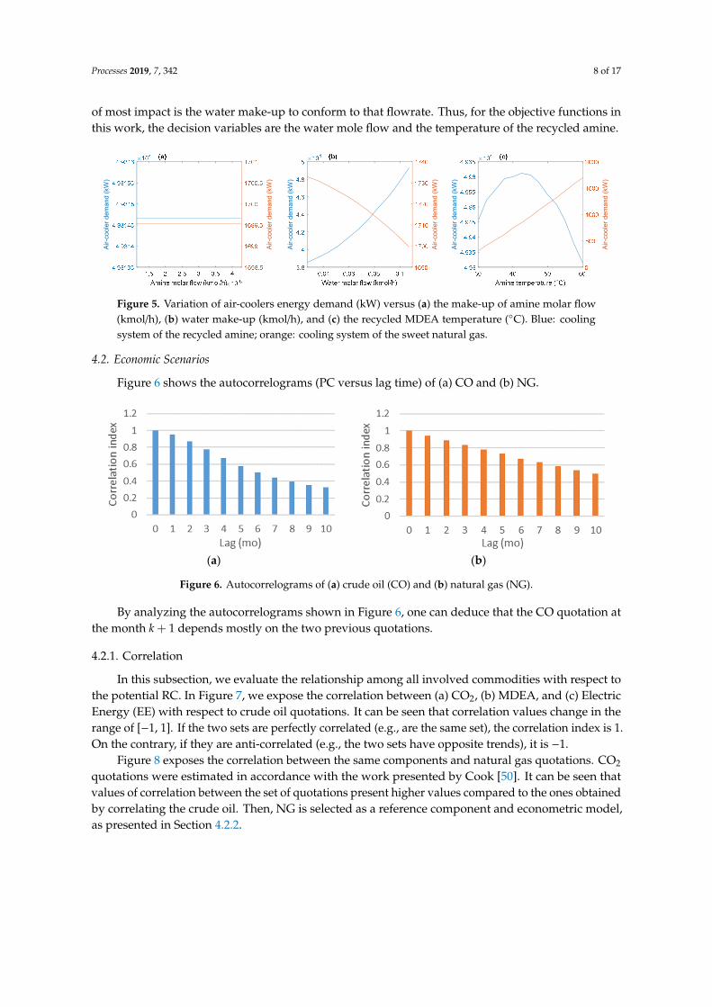
Figure 5. Variation of air-coolers energy demand (kW) versus (a) the make-up of amine molar flow (kmol/h), (b) water make-up (kmol/h), and (c) the recycled MDEA temperature (°C). Blue: cooling system of the recycled amine; orange: cooling system of the sweet natural gas.

Figures 2–5 expose a remarkable dependency between the main energy consumptions and the temperature of the recycled MDEA. Moreover, it was illustrated that the energy requirements strongly depend on the flow rate of the water make up. On the other hand, the variation of the MDEA flow rate proves to not alter the energy requirement of the reboiler, condenser, compressors, and the air-coolers. With this analysis, it is demonstrated that the proper DoF, representing the reduction of the recycle MDEA flow rate, corresponds to the water makeup of the process. Previous articles state that the decision variable is the recycled aqueous amine flowrate, but it is demonstrated here that the variable of most impact is the water make-up to conform to that flowrate. Thus, for the objective functions in this work, the decision variables are the water mole flow and the temperature of the recycled amine.

4.2. Economic Scenarios

Figure 6 shows the autocorrelograms (PC versus lag time) of (a) CO and (b) NG.

(a) (b)

Figure 6. Autocorrelograms of (a) crude oil (CO) and (b) natural gas (NG).

By analyzing the autocorrelograms shown in Figure 6, one can deduce that the CO quotation at the month 𝑘 + 1 depends mostly on the two previous quotations.

4.2.1. Correlation

In this subsection, we evaluate the relationship among all involved commodities with respect to the potential RC. In Figure 7, we expose the correlation between (a) CO2, (b) MDEA, and (c) Electric Energy (EE) with respect to crude oil quotations. It can be seen that correlation values change in the

Air-c

oole

r dem

and

(kW

)

Air-c

oole

r dem

and

(kW

)

Air-c

oole

r dem

and

(kW

)

Air-c

oole

r dem

and

(kW

)

Air-c

oole

r dem

and

(kW

)

Air-c

oole

r dem

and

(kW

)

Figure 5. Variation of air-coolers energy demand (kW) versus (a) the make-up of amine molar flow(kmol/h), (b) water make-up (kmol/h), and (c) the recycled MDEA temperature (◦C). Blue: coolingsystem of the recycled amine; orange: cooling system of the sweet natural gas.

4.2. Economic Scenarios

Figure 6 shows the autocorrelograms (PC versus lag time) of (a) CO and (b) NG.

Processes 2019, 7, x FOR PEER REVIEW 8 of 17

101) versus (a) the flow rate of the make-up of MDEA, (b) the make-up of water, and (c) the temperature of the recycled amine.

Figure 5. Variation of air-coolers energy demand (kW) versus (a) the make-up of amine molar flow (kmol/h), (b) water make-up (kmol/h), and (c) the recycled MDEA temperature (°C). Blue: cooling system of the recycled amine; orange: cooling system of the sweet natural gas.

Figures 2–5 expose a remarkable dependency between the main energy consumptions and the temperature of the recycled MDEA. Moreover, it was illustrated that the energy requirements strongly depend on the flow rate of the water make up. On the other hand, the variation of the MDEA flow rate proves to not alter the energy requirement of the reboiler, condenser, compressors, and the air-coolers. With this analysis, it is demonstrated that the proper DoF, representing the reduction of the recycle MDEA flow rate, corresponds to the water makeup of the process. Previous articles state that the decision variable is the recycled aqueous amine flowrate, but it is demonstrated here that the variable of most impact is the water make-up to conform to that flowrate. Thus, for the objective functions in this work, the decision variables are the water mole flow and the temperature of the recycled amine.

4.2. Economic Scenarios

Figure 6 shows the autocorrelograms (PC versus lag time) of (a) CO and (b) NG.

(a) (b)

Figure 6. Autocorrelograms of (a) crude oil (CO) and (b) natural gas (NG).

By analyzing the autocorrelograms shown in Figure 6, one can deduce that the CO quotation at the month 𝑘 + 1 depends mostly on the two previous quotations.

4.2.1. Correlation

In this subsection, we evaluate the relationship among all involved commodities with respect to the potential RC. In Figure 7, we expose the correlation between (a) CO2, (b) MDEA, and (c) Electric Energy (EE) with respect to crude oil quotations. It can be seen that correlation values change in the

Air-c

oole

r dem

and

(kW

)

Air-c

oole

r dem

and

(kW

)

Air-c

oole

r dem

and

(kW

)

Air-c

oole

r dem

and

(kW

)

Air-c

oole

r dem

and

(kW

)

Air-c

oole

r dem

and

(kW

)Figure 6. Autocorrelograms of (a) crude oil (CO) and (b) natural gas (NG).

By analyzing the autocorrelograms shown in Figure 6, one can deduce that the CO quotation atthe month k + 1 depends mostly on the two previous quotations.

4.2.1. Correlation

In this subsection, we evaluate the relationship among all involved commodities with respect tothe potential RC. In Figure 7, we expose the correlation between (a) CO2, (b) MDEA, and (c) ElectricEnergy (EE) with respect to crude oil quotations. It can be seen that correlation values change in therange of [−1, 1]. If the two sets are perfectly correlated (e.g., are the same set), the correlation index is 1.On the contrary, if they are anti-correlated (e.g., the two sets have opposite trends), it is −1.

Figure 8 exposes the correlation between the same components and natural gas quotations. CO2

quotations were estimated in accordance with the work presented by Cook [50]. It can be seen thatvalues of correlation between the set of quotations present higher values compared to the ones obtainedby correlating the crude oil. Then, NG is selected as a reference component and econometric model,as presented in Section 4.2.2.

Processes 2019, 7, 342 9 of 17

Processes 2019, 7, x FOR PEER REVIEW 9 of 17

range of [−1,1]. If the two sets are perfectly correlated (e.g., are the same set), the correlation index is 1. On the contrary, if they are anti-correlated (e.g., the two sets have opposite trends), it is −1.

(a) (b) (c)

Figure 7. Correlation between CO and (a) CO2, (b) MDEA, and (c) electricity quotations.

Figure 8 exposes the correlation between the same components and natural gas quotations. CO2 quotations were estimated in accordance with the work presented by Cook [50]. It can be seen that values of correlation between the set of quotations present higher values compared to the ones obtained by correlating the crude oil. Then, NG is selected as a reference component and econometric model, as presented in Section 4.2.2.

(a) (b) (c)

Figure 8. Correlation between NG and (a) CO2, (b) MDEA, and (c) electricity quotations.

4.2.2. Econometric Models

From Figures 7 and 8, we observe better correlation indexes when comparing to the NG quotations. Then, the EM of NG as RC becomes the one expressed through Equation (5).

Where 𝑃 , is the monthly quotation of NG. 𝜎 and 𝑃 are the standard deviation of the prices and the average of relative errors, respectively. 𝑟𝑎𝑛𝑑 is a stochastic function normally distributed, and 𝐴, 𝐵, and 𝐶 are adaptive parameters calculated with linear regression, minimizing the square error between real quotations and those predicted by the model [51].

Manca [38] reports EM for toluene, benzene, propylene, and cumene prices based on a dedicated (auto)correlogram analysis. According to our correlation indexes, we elaborate the EM for the CO2 conditioning process. Table 1 presents Autoregressive Distributed Lag (ADL) models for estimating each quotation evolution, without the stochastic factor. 𝑃 , = 𝐴 + 𝐵 ∙ 𝑃 , + 𝐶 ∙ 𝑃 , ∙ (1 + 𝑟𝑎𝑛𝑑 ∙ 𝜎 + 𝑃 ). (5)

Figure 7. Correlation between CO and (a) CO2, (b) MDEA, and (c) electricity quotations.

Processes 2019, 7, x FOR PEER REVIEW 9 of 17

range of [−1,1]. If the two sets are perfectly correlated (e.g., are the same set), the correlation index is 1. On the contrary, if they are anti-correlated (e.g., the two sets have opposite trends), it is −1.

(a) (b) (c)

Figure 7. Correlation between CO and (a) CO2, (b) MDEA, and (c) electricity quotations.

Figure 8 exposes the correlation between the same components and natural gas quotations. CO2 quotations were estimated in accordance with the work presented by Cook [50]. It can be seen that values of correlation between the set of quotations present higher values compared to the ones obtained by correlating the crude oil. Then, NG is selected as a reference component and econometric model, as presented in Section 4.2.2.

(a) (b) (c)

Figure 8. Correlation between NG and (a) CO2, (b) MDEA, and (c) electricity quotations.

4.2.2. Econometric Models

From Figures 7 and 8, we observe better correlation indexes when comparing to the NG quotations. Then, the EM of NG as RC becomes the one expressed through Equation (5).

Where 𝑃 , is the monthly quotation of NG. 𝜎 and 𝑃 are the standard deviation of the prices and the average of relative errors, respectively. 𝑟𝑎𝑛𝑑 is a stochastic function normally distributed, and 𝐴, 𝐵, and 𝐶 are adaptive parameters calculated with linear regression, minimizing the square error between real quotations and those predicted by the model [51].

Manca [38] reports EM for toluene, benzene, propylene, and cumene prices based on a dedicated (auto)correlogram analysis. According to our correlation indexes, we elaborate the EM for the CO2 conditioning process. Table 1 presents Autoregressive Distributed Lag (ADL) models for estimating each quotation evolution, without the stochastic factor. 𝑃 , = 𝐴 + 𝐵 ∙ 𝑃 , + 𝐶 ∙ 𝑃 , ∙ (1 + 𝑟𝑎𝑛𝑑 ∙ 𝜎 + 𝑃 ). (5)

Figure 8. Correlation between NG and (a) CO2, (b) MDEA, and (c) electricity quotations.

4.2.2. Econometric Models

From Figures 7 and 8, we observe better correlation indexes when comparing to the NG quotations.Then, the EM of NG as RC becomes the one expressed through Equation (5).

Where PNG,k+1 is the monthly quotation of NG. σ and P are the standard deviation of the pricesand the average of relative errors, respectively. rand is a stochastic function normally distributed, andA, B, and C are adaptive parameters calculated with linear regression, minimizing the square errorbetween real quotations and those predicted by the model [51].

Manca [38] reports EM for toluene, benzene, propylene, and cumene prices based on a dedicated(auto)correlogram analysis. According to our correlation indexes, we elaborate the EM for the CO2

conditioning process. Table 1 presents Autoregressive Distributed Lag (ADL) models for estimatingeach quotation evolution, without the stochastic factor.

PNG,k+1 =(A + B·PNG,k + C·PNG,k−1

)·

(1 + rand·σNG + PNG

). (7)

Table 1. ADL EM for NG, CO2, and MDEA prices, without the stochastic factor.

Component Model

CO2 PCO2,k+1 = A + B·PNG,k+1 + C·PCO2,k + D·PCO2,k−1MDEA PMDEA,k+1 = A + B·PNG,k+1 + C·PMDEA,k + D·PMDEA,k−1

To simply the forecast EE quotations, we adopt previous monthly prices of the Ministry ofEnergy [41]. Similar to Manca [52], the EM for EE is based on (auto)correlograms and the economicdependency of the EE to NG. From these observations, it is feasible to apply the model represented byEquation (8):

PEE,k+1 = A + B·PNG,k + C·PEE,k (8)

Processes 2019, 7, 342 10 of 17

where the price of EE (PEE,k+1) is estimated employing previous quotations of NG and EE. Table 2reports the adaptive coefficients, including the models of NG, CO2, MDEA, and EE.

Table 2. Adaptive parameters of ADL EM of NG, CO2, and MDEA.

Component A B C D σ P

NG 0.0362 −0.0285 1.2205 - 0.1918 0.0705CO2 0.0033 0.0078 1.4167 −0.4870 0.0606 0.0074

MDEA 0.1124 0.9731 0 −0.0171 0.0126 0.0002

We use the EM of CO2, MDEA and EE to generate a set of random economic scenarios. Figure 9shows eight predicted trajectories from the EM of NG, MDEA, CO2, and EE, during a time horizon of120 months, in different random colors. It shows a probabilistic approach, based on a distribution ofmultiple viable economic scenarios.Processes 2019, 7, x FOR PEER REVIEW 11 of 17

Figure 9. Random price trajectories, for (a) NG expressed, (b) MDEA, (c) CO2, and (d) EE.

4.3. Optimal Economic and Environmental Friendly Design

Results concerning the optimal design of the CO2 separation plant are shown in this section.

4.3.1. DEP4 cumulated

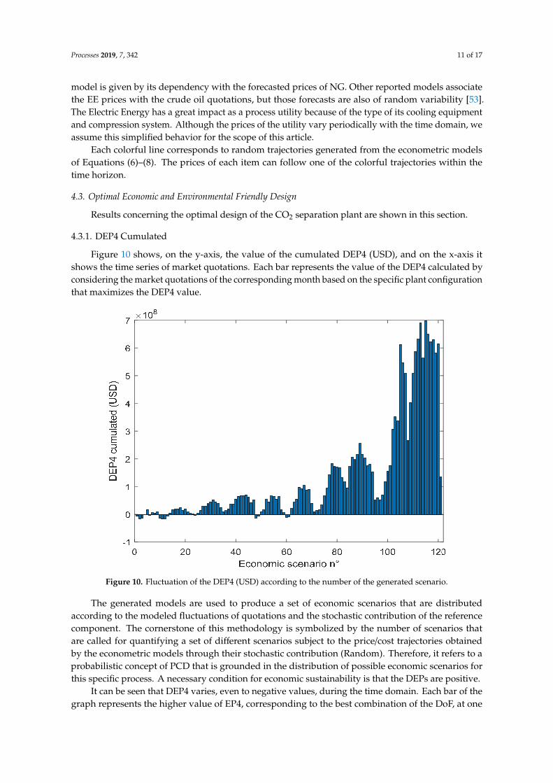
Figure 10 shows, on the y-axis, the value of the cumulated DEP4 (USD), and on the x-axis it shows the time series of market quotations. Each bar represents the value of the DEP4 calculated by considering the market quotations of the corresponding month based on the specific plant configuration that maximizes the DEP4 value.

The generated models are used to produce a set of economic scenarios that are distributed according to the modeled fluctuations of quotations and the stochastic contribution of the reference component. The cornerstone of this methodology is symbolized by the number of scenarios that are called for quantifying a set of different scenarios subject to the price/cost trajectories obtained by the econometric models through their stochastic contribution (Random). Therefore, it refers to a probabilistic concept of PCD that is grounded in the distribution of possible economic scenarios for this specific process. A necessary condition for economic sustainability is that the DEPs are positive.

Pric

e (U

SD/m

3)Pr

ice

(USD

/kg)

Pric

e (U

SD/m

3)Pr

ice

(USD

/MW

h)

Figure 9. Random price trajectories, for (a) NG expressed, (b) MDEA, (c) CO2, and (d) EE.

Particularly for the case of the Electric Energy (Figure 9d), we present a brief predictive modelwhere A = 2.98, B = 1.316, and C = 0.81 (Sepiacci et al. [16]), in Equation (8). The predictive nature of this

Processes 2019, 7, 342 11 of 17

model is given by its dependency with the forecasted prices of NG. Other reported models associatethe EE prices with the crude oil quotations, but those forecasts are also of random variability [53].The Electric Energy has a great impact as a process utility because of the type of its cooling equipmentand compression system. Although the prices of the utility vary periodically with the time domain, weassume this simplified behavior for the scope of this article.

Each colorful line corresponds to random trajectories generated from the econometric modelsof Equations (6)–(8). The prices of each item can follow one of the colorful trajectories within thetime horizon.

4.3. Optimal Economic and Environmental Friendly Design

Results concerning the optimal design of the CO2 separation plant are shown in this section.

4.3.1. DEP4 Cumulated

Figure 10 shows, on the y-axis, the value of the cumulated DEP4 (USD), and on the x-axis itshows the time series of market quotations. Each bar represents the value of the DEP4 calculated byconsidering the market quotations of the corresponding month based on the specific plant configurationthat maximizes the DEP4 value.

Processes 2019, 7, x FOR PEER REVIEW 12 of 17

Figure 10. Fluctuation of the DEP4 (USD) according to the number of the generated scenario.

It can be seen that DEP4 varies, even to negative values, during the time domain. Each bar of the graph represents the higher value of EP4, corresponding to the best combination of the DoF, at one particular month. In general, the economic potential fluctuation strongly depends on the price volatility of raw materials and final products. Where positive, the obtained DEP4 is of an eight-power magnitude, which demonstrates the economic potential of the plant in accordance with the predictive models.

4.3.2. Economic Optimal

Figure 11 illustrates the trend of the cumulated DEP4 as a function of the DoF, the water flow make-up, and the temperature of the recycled amine. The presented surface represents the maximization of Equation (4), where a total capital expenditure of 1.44 × 107 USD is estimated from the calculation. As previously stated, the DEP4 is not represented by a single value but by a distribution of values, one for each scenario. In order to have a simple representation of the economic objective function, we present the average value of the cumulated DEP4. The results of Equation (4) show that the average of the cumulated DEP4 reaches eight order values.

The configuration yielding the maximum value of the cumulated DEP4 corresponds to a temperature equal to 60 °C for the MDEA to recycle and value the water amine flow rate equal to 0.0274 kmol/h.

Based on this experience, high temperatures of MDEA imply that the conversion of the absorption reaction is increased and, consequently, the produced CO2 is increased. Interestingly, an increment of the water flow rate proves that the MDEA concentration of 38 wt% can be modified to obtain a better performance in terms of the economical aspect of this process. At the same value of temperature, 60 °C, and 0.1074 kmol/h, the cumulated DEP4 is equal to 1.06 × 108 USD. The order of magnitude of this DEP4 is even higher than the one obtained by Sepiacci et al. [16], who obtained a six-order DEP4 while applying this methodology in a petrochemical process.

Figure 10. Fluctuation of the DEP4 (USD) according to the number of the generated scenario.

The generated models are used to produce a set of economic scenarios that are distributedaccording to the modeled fluctuations of quotations and the stochastic contribution of the referencecomponent. The cornerstone of this methodology is symbolized by the number of scenarios thatare called for quantifying a set of different scenarios subject to the price/cost trajectories obtainedby the econometric models through their stochastic contribution (Random). Therefore, it refers to aprobabilistic concept of PCD that is grounded in the distribution of possible economic scenarios forthis specific process. A necessary condition for economic sustainability is that the DEPs are positive.

It can be seen that DEP4 varies, even to negative values, during the time domain. Each bar of thegraph represents the higher value of EP4, corresponding to the best combination of the DoF, at one

Processes 2019, 7, 342 12 of 17

particular month. In general, the economic potential fluctuation strongly depends on the price volatilityof raw materials and final products. Where positive, the obtained DEP4 is of an eight-power magnitude,which demonstrates the economic potential of the plant in accordance with the predictive models.

4.3.2. Economic Optimal

Figure 11 illustrates the trend of the cumulated DEP4 as a function of the DoF, the water flowmake-up, and the temperature of the recycled amine. The presented surface represents the maximizationof Equation (4), where a total capital expenditure of 1.44 × 107 USD is estimated from the calculation.As previously stated, the DEP4 is not represented by a single value but by a distribution of values,one for each scenario. In order to have a simple representation of the economic objective function, wepresent the average value of the cumulated DEP4. The results of Equation (4) show that the average ofthe cumulated DEP4 reaches eight order values.

The configuration yielding the maximum value of the cumulated DEP4 corresponds to atemperature equal to 60 ◦C for the MDEA to recycle and value the water amine flow rate equalto 0.0274 kmol/h.

Based on this experience, high temperatures of MDEA imply that the conversion of the absorptionreaction is increased and, consequently, the produced CO2 is increased. Interestingly, an increment ofthe water flow rate proves that the MDEA concentration of 38 wt% can be modified to obtain a betterperformance in terms of the economical aspect of this process. At the same value of temperature, 60 ◦C,and 0.1074 kmol/h, the cumulated DEP4 is equal to 1.06 × 108 USD. The order of magnitude of thisDEP4 is even higher than the one obtained by Sepiacci et al. [16], who obtained a six-order DEP4 whileapplying this methodology in a petrochemical process.

4.3.3. Minimal Environmental Risks

Figure 12 shows the behavior of the PEI. In this case, the highest environmental risk is observed atthe upper bounds of the DoF.

A probabilistic approach to future scenarios is concerned to find the combination of decisive DoFthat maximizes the indicator of economic sustainability. Similarly, the potential environmental risk isalso evaluated. Results show that this CO2 separation design is promising, although the PEI indicatesthat the higher the profitability, the larger the environmental risk is. The environmental risk appears athigh values of water make-up flow and recycle amine temperatures. This situation may be explainedby the toxicological aspects of the involved chemicals within the process—an increase in the power ofthe cooling stage and modification of the reboiler combustion parameters.

Processes 2019, 7, 342 13 of 17Processes 2019, 7, x FOR PEER REVIEW 13 of 17

(a)

(b)

Figure 11 (a-b). Average cumulated DEP4 (USD) function with respect to water amine molar flow rate (kmol/h) and recycle MDEA temperature (°C), based on the PCD method.

4.3.3. Minimal Environmental Risks

Figure 12 shows the behavior of the PEI. In this case, the highest environmental risk is observed at the upper bounds of the DoF.

Figure 11. (a,b). Average cumulated DEP4 (USD) function with respect to water amine molar flow rate(kmol/h) and recycle MDEA temperature (◦C), based on the PCD method.

Processes 2019, 7, 342 14 of 17Processes 2019, 7, x FOR PEER REVIEW 14 of 17

(a)

(b)

Figure 12 (a-b). PEI function with respect to water amine molar flow rate (kmol/h) and recycle MDEA temperature (°C), based on Waste Reduction.

A probabilistic approach to future scenarios is concerned to find the combination of decisive DoF that maximizes the indicator of economic sustainability. Similarly, the potential environmental risk is also evaluated. Results show that this CO2 separation design is promising, although the PEI indicates that the higher the profitability, the larger the environmental risk is. The environmental risk appears at high values of water make-up flow and recycle amine temperatures. This situation may be explained by the toxicological aspects of the involved chemicals within the process—an increase in the power of the cooling stage and modification of the reboiler combustion parameters.

Figure 12. (a,b). PEI function with respect to water amine molar flow rate (kmol/h) and recycle MDEAtemperature (◦C), based on Waste Reduction.

5. Conclusions and Future Developments

This paper evaluates the process to obtain and condition CO2 to be used as an EOR fluid, in theArgentine Basin of Neuquén. We focus the study on the evaluation of economic aspects in a context ofmarket variability and price uncertainties. PCD methodology is adopted to achieve the aim of thearticle. With this technique, a probabilistic approach to future scenarios is used to find the combinationof decisive DoF that maximizes the indicator of economic sustainability. According to the results,

Processes 2019, 7, 342 15 of 17

the implementation of the plant at this stage of the study is feasible and suggests promising values forrevenues and economic profitability.

The results of this preliminary study are promising. The economic potential of the four order isproven to be high, with a magnitude of eight order in USD/y. Further, the statistical indexes prove thatthe plant is profitable within 12 years of the process time’s life. Finally, the conditions of the plantmaximizing the EP are identified—a recycle amine flow of 0.0274 kmol/h at 60 ◦C proved to be anoptimal combination of the decision variables. In respect to the ‘green’ risks, it is demonstrated thatthe higher the upper bounds of the DoF, the higher the environmental risk is.

The evaluation of DoF and their impact on the energy requirements of the plant have led to anotable conclusion—the decision variable affecting the consumer is the water makeup of the plant.Thus, a new perspective for authors working with a similar process is presented in this paper.

Future work can extend the limits of this methodology and include a higher number of DoFs, suchas the ones related to the regeneration of the column, which is rarely discussed in the bibliography.In addition, the economic potential evaluation can be extended with heat integration coming from thepinch technology.

The last important aspect to be noted is that the CO2 was historically considered to be a by-product,and in the past, it was a common practice to flare it. However, the recuperation and condition of thisgas, and the installation of a proper plant operating at proper conditions, might be the starting pointfor implementing the technology of EOR in the region, taking into account volatile market scenarios.

Author Contributions: Conceptualization, J.P.G., E.E. and D.M.; Methodology, J.P.G., E.E. and D.M.; Validation,J.P.G., E.E. and D.M.; Investigation, J.P.G., E.E. and D.M.; Resources, E.E. and D.M.; Writing-Original DraftPreparation, J.P.G. and E.E.; Writing-Review & Editing, J.P.G., E.E. and D.M.; Supervision, E.E. and D.M.; FundingAcquisition, J.P.G., E.E. and D.M.

Funding: This publication has been produced with the funding of the ERASMUS MUNDUS (Action 2 Strand 1)SUSTAIN-T Program, under the coordination of Politecnico di Milano, Italy. The authors also acknowledge thefunding of CONICET (Grant 2222016000218900) and the Universidad Nacional de Salta (CIUNSa Projects 2253/0,2465, and 2645), Argentina.

Conflicts of Interest: The authors declare no conflict of interest.

References

1. Roussanaly, S.; Grimstad, A.-A. The Economic Value of CO2 for EOR Applications. Energy Procedia 2014, 63,7836–7843. [CrossRef]

2. Yang, H.; Xu, Z.; Fan, M.; Gupta, R.; Slimane, R.B.; Bland, A.E.; Wright, I. Progress in carbon dioxideseparation and capture: A review. J. Environ. Sci. 2008, 20, 14–27. [CrossRef]

3. Haszeldine, R.S. Carbon capture and storage: How green can black be? Science 2009, 325, 1647–1652.[CrossRef] [PubMed]

4. Wright, I.W.; Lee, A.; Middleton, P.; Lowe, C.; Imbus, S.W.; Miracca, I. CO2 Capture Project: Initial Results.In Proceedings of the SPE International Conference on Health, Safety, and Environment in Oil and GasExploration and Production, Society of Petroleum Engineers, Calgary, AB, Canada, 29–31 March 2004.

5. Mumford, K.A.; Wu, Y.; Smith, K.H.; Stevens, G.W. Review of solvent based carbon-dioxide capturetechnologies. Front. Chem. Sci. Eng. 2015, 9, 125–141. [CrossRef]

6. Brush, R.M.; Davitt, H.J.; Aimar, O.B.; Arguello, J.; Whiteside, J.M. Immiscible CO2 flooding for increasedoil recovery and reduced emissions. In Proceedings of the SPE/DOE Improved Oil Recovery Symposium,Society of Petroleum Engineers, Tulsa, Oklahoma, 3–5 April 2000.

7. Mazzetti, M.J.; Skagestad, R.; Mathisen, A.; Eldrup, N.H. CO2 from natural gas sweetening to kick-start EORin the North Sea. Energy Procedia 2014, 63, 7280–7289. [CrossRef]

8. Herzog, H.J. Scaling up carbon dioxide capture and storage: From megatons to gigatons. Energy Econ. 2011,33, 597–604. [CrossRef]

9. Kwak, D.-H.; Yun, D.; Binns, M.; Yeo, Y.-K.; Kim, J.-K. Conceptual process design of CO2 recovery plants forenhanced oil recovery applications. Ind. Eng. Chem. Res. 2014, 53, 14385–14396. [CrossRef]

Processes 2019, 7, 342 16 of 17

10. Leung, D.Y.; Caramanna, G.; Maroto-Valer, M.M. An overview of current status of carbon dioxide captureand storage technologies. Renew. Sustain. Energy Rev. 2014, 39, 426–443. [CrossRef]

11. Chávez-Rodríguez, M.; Varela, D.; Rodrigues, F.; Salvagno, J.B.; Köberle, A.C.; Vasquez-Arroyo, E.; Raineri, R.;Rabinovich, G. The role of LNG and unconventional gas in the future natural gas markets of Argentina andChile. J. Nat. Gas Sci. Eng. 2017, 45, 584–598. [CrossRef]

12. Ponzo, R.; Dyner, I.; Arango, S.; Larsen, E.R. Regulation and development of the Argentinean gas market.Energy Policy 2011, 39, 1070–1079. [CrossRef]

13. Manolas, D.A.; Frangopoulos, C.A.; Gialamas, T.P.; Tsahalis, D.T. Operation optimization of an industrialcogeneration system by a genetic algorithm. Energy Convers. Manag. 1997, 38, 1625–1636. [CrossRef]

14. Douglas, J.M. Conceptual Design of Chemical Processes; McGraw-Hill: New York, NY, USA, 1988; Volume 1110.15. Harmsen, G. Industrial best practices of conceptual process design. Chem. Eng. Process. Process Intensif. 2004,

43, 671–675. [CrossRef]16. Sepiacci, P.; Depetri, V.; Manca, D. A systematic approach to the optimal design of chemical plants with

waste reduction and market uncertainty. Comput. Chem. Eng. 2017, 102, 96–109. [CrossRef]17. Manca, D.; Grana, R. Dynamic conceptual design of industrial processes. Comput. Chem. Eng. 2010, 34,

656–667. [CrossRef]18. Cabezas, H.; Bare, J.C.; Mallick, S.K. Pollution prevention with chemical process simulators: The generalized

waste reduction (WAR) algorithm—Full version. Comput. Chem. Eng. 1999, 23, 623–634. [CrossRef]19. Gutierrez, J.P.; Ruiz, E.L.A.; Erdmann, E. Energy requirements, GHG emissions and investment costs in

natural gas sweetening processes. J. Nat. Gas Sci. Eng. 2017, 38, 187–194. [CrossRef]20. Gallo, G.; Erdmann, E. Potencialidad el EOR con CO2 en reservorios de baja permeabilidad de la cuenca

Neuquina. In Congreso de Produccion y Desarrollo de Reservas; Instituto Argentino del Petroleo y Gas: BuenosAires, Argentina, 2016.

21. Mores, P.; Scenna, N.; Mussati, S. Post-combustion CO2 capture process: Equilibrium stage mathematicalmodel of the chemical absorption of CO2 into monoethanolamine (MEA) aqueous solution. Chem. Eng. Res.Des. 2011, 89, 1587–1599. [CrossRef]

22. Young, D.; Scharp, R.; Cabezas, H. The waste reduction (WAR) algorithm: Environmental impacts, energyconsumption, and engineering economics. Waste Manag. 2000, 20, 605–615. [CrossRef]

23. Erdmann, E.; Ruiz, L.A.; Martínez, J.; Gutierrez, J.P.; Tarifa, E. Endulzamiento de gas natural con aminas.Simulación del proceso y análisis de sensibilidad paramétrico. Avances en Ciencias e Ingeniería. 2012, 3,89–101.

24. Green, D.W.; Perry, R.H. Chemical Engineers’ Handbook; McGraw-Hill: New York, NY, USA, 1973.25. Fouad, W.A.; Berrouk, A.S. Using mixed tertiary amines for gas sweetening energy requirement reduction.

J. Nat. Gas Sci. Eng. 2013, 11, 12–17. [CrossRef]26. Kazemi, A.; Malayeri, M.; kharaji, A.G.; Shariati, A. Feasibility study, simulation and economical evaluation

of natural gas sweetening processes—Part 1: A case study on a low capacity plant in iran. J. Nat. Gas Sci.Eng. 2014, 20, 16–22. [CrossRef]

27. Gutierrez, J.P.; Benitez, L.A.; Ale Ruiz, E.L.; Erdmann, E. A sensitivity analysis and a comparison of twosimulators performance for the process of natural gas sweetening. J. Nat. Gas Sci. Eng. 2016, 31, 800–807.[CrossRef]

28. Al-Lagtah, N.M.; Al-Habsi, S.; Onaizi, S.A. Optimization and performance improvement of Lekhwair naturalgas sweetening plant using Aspen HYSYS. J. Nat. Gas Sci. Eng. 2015, 26, 367–381. [CrossRef]

29. Kvamsdal, H.; Jakobsen, J.; Hoff, K. Dynamic modeling and simulation of a CO2 absorber column forpost-combustion CO2 capture. Chem. Eng. Process. Process Intensif. 2009, 48, 135–144. [CrossRef]

30. Prölss, K.; Tummescheit, H.; Velut, S.; Åkesson, J. Dynamic model of a post-combustion absorption unit foruse in a non-linear model predictive control scheme. Energy Procedia 2011, 4, 2620–2627. [CrossRef]

31. Behroozsarand, A.; Zamaniyan, A. Multiobjective optimization scheme for industrial synthesis gas sweeteningplant in GTL process. J. Nat. Gas Chem. 2011, 20, 99–109. [CrossRef]

32. Øi, L.E.; Bråthen, T.; Berg, C.; Brekne, S.K.; Flatin, M.; Johnsen, R.; Moen, I.G.; Thomassen, E. Optimizationof configurations for amine based CO2 absorption using Aspen HYSYS. Energy Procedia 2014, 51, 224–233.[CrossRef]

Processes 2019, 7, 342 17 of 17

33. Gutierrez, J.P.; Erdmann, E.; Manca, D. Multi-objective optimization of a CO2-EOR process from thesustainability criteria. In 28th European Symposium on Computer Aided Process Engineering; Elsevier: Graz,Austria, 2018.

34. Honeywell. UniSim Design; Honeywell International Inc.: Charlotte, NC, USA, 2016.35. Muhammad, A.; GadelHak, Y. Correlating the additional amine sweetening cost to acid gases load in natural

gas using Aspen Hysys. J. Nat. Gas Sci. Eng. 2014, 17, 119–130. [CrossRef]36. Torres-Ortega, C.E.; Segovia-Hernández, J.G.; Gómez-Castro, F.I.; Hernández, S.; Bonilla-Petriciolet, A.;

Rong, B.-G.; Errico, M. Design, optimization and controllability of an alternative process based on extractivedistillation for an ethane–carbon dioxide mixture. Chem. Eng. Process. Process Intensif. 2013, 74, 55–68.[CrossRef]

37. Manca, D. A methodology to forecast the price of commodities. In Computer Aided Chemical Engineering;Karimi, I.A., Srinivasan, R., Eds.; Elsevier: Amsterdam, The Netherlands, 2012; pp. 1306–1310.

38. Manca, D. Modeling the commodity fluctuations of OPEX terms. Comput. Chem. Eng. 2013, 57, 3–9.[CrossRef]

39. Sepiacci, P.; Manca, D. Economic assessment of chemical plants supported by environmental and socialsustainability. Chem. Eng. Trans. 2015, 43, 2209–2214.

40. EIA. US Energy Information Administration. 2018. Available online: https://www.eia.gov/ (accessed on1 June 2018).

41. Ministry-of-Energy. Reporte de Produccion. 2017; Presidencia de la Nacion Argentina. Available online:https://www.se.gob.ar/ (accessed on 1 June 2018).

42. Wiggins, S.; Etienne, X.L. Turbulent times: Uncovering the origins of US natural gas price fluctuations sincederegulation. Energy Econ. 2017, 64, 196–205. [CrossRef]

43. Zhou, H.; Deng, Z.; Xia, Y.; Fu, M. A new sampling method in particle filter based on Pearson correlationcoefficient. Neurocomputing 2016, 216, 208–215. [CrossRef]

44. Lee Rodgers, J.; Nicewander, W.A. Thirteen ways to look at the correlation coefficient. Am. Stat. 1988, 42,59–66. [CrossRef]

45. Mohamed Salleh, F.H.; Arif, S.M.; Zainudin, S.; Firdaus-Raih, M. Reconstructing gene regulatory networksfrom knock-out data using Gaussian Noise Model and Pearson Correlation Coefficient. Comput. Biol. Chem.2015, 59, 3–14. [CrossRef] [PubMed]

46. Dancey, C.P.; Reidy, J. Statistics without Maths for Psychology; Pearson Education: London, UK, 2007.47. Young, D.; Cabezas, H. Designing sustainable processes with simulation: The waste reduction (WAR)

algorithm. Comput. Chem. Eng. 1999, 23, 1477–1491. [CrossRef]48. Marticorena, A.A.; Mandagarán, B.A.; Campanella, E.A. Análisis del Impacto Ambiental de la Recuperación

de Metanol en la Producción de Biodiesel usando el Algoritmo de Reducción de Desechos WAR. Inf. Tecnol.2010, 21, 23–30. [CrossRef]

49. Barrett, W.M.; van Baten, J.; Martin, T. Implementation of the waste reduction (WAR) algorithm utilizingflowsheet monitoring. Comput. Chem. Eng. 2011, 35, 2680–2686. [CrossRef]

50. Cook, B. EORI’s Economic scoping model. In Proceedings of the 8th Annual EORI Casper CO2 Conference,Enhanced Oil Recovery Institute, University of Wyoming, Laramie, WY, USA, 9 July 2014.

51. Mazzetto, F.; Ortiz-Gutiérrez, R.A.; Manca, D.; Bezzo, F. Strategic design of bioethanol supply chainsincluding commodity market dynamics. Ind. Eng. Chem. Res. 2013, 52, 10305–10316. [CrossRef]

52. Manca, D. Price model of electrical energy for PSE applications. Comput. Chem. Eng. 2016, 84, 208–216.[CrossRef]

53. Manca, D. A methodology to forecast the price of electric energy. In Computer Aided Chemical Engineering;Elsevier: Amsterdam, The Netherlands, 2013; pp. 679–684.

© 2019 by the authors. Licensee MDPI, Basel, Switzerland. This article is an open accessarticle distributed under the terms and conditions of the Creative Commons Attribution(CC BY) license (http://creativecommons.org/licenses/by/4.0/).