processing and classifying satellite imagery to in the nelson area … · 2017-01-19 · processing...

Processing and classifying satellite imagery to assess the December 2011 landslide storm damage in the Nelson area

S. Ashraf K. E. Jones GNS Science Consultancy Report 2013/13 January 2013

Project number 440W1472

DISCLAIMER

This report has been prepared by the Institute of Geological and Nuclear Sciences Limited (GNS Science) exclusively for and under contract to Nelson City Council. Unless otherwise agreed in writing by GNS Science, GNS Science accepts no responsibility for any use of, or reliance on any contents of this Report by any person other than Nelson City Council and shall not be liable to any person other than Nelson City Council, on any ground, for any loss, damage or expense arising from such use or reliance.

The data presented in this Report are available to GNS Science for other use from February 2013.

BIBLIOGRAPHIC REFERENCE

Ashraf, S.; Jones, K.E. 2013. Processing and classifying WV-2 satellite imagery to assess the December 2011 landslide storm damage in the Nelson area, GNS Science Consultancy Report 2013/13. 19 p + CD.

Confidential 2013

GNS Science Consultancy Report 2013/13 i

CONTENTS

EXECUTIVE SUMMARY ....................................................................................................... iii

1.0 INTRODUCTION ........................................................................................................ 1

1.1 Project Objectives.......................................................................................................... 2 1.2 Project Deliverables....................................................................................................... 2

2.0 METHODOLOGY ....................................................................................................... 3

2.1 Post event imagery ........................................................................................................ 3 2.2 Data import and ortho-rectification ................................................................................ 5 2.3 Conversion to reflectance data ...................................................................................... 7 2.4 Mosaicking and image fusion ........................................................................................ 9 2.5 Spectral classification .................................................................................................. 13

3.0 RESULTS ................................................................................................................. 15

3.1 Differentiating between scar and debris trail ............................................................... 17 3.2 Accuracy assessment ................................................................................................. 17 3.3 Limitations of satellite imagery .................................................................................... 17

4.0 ACKNOWLEDGEMENT ........................................................................................... 19

5.0 REFERENCES ......................................................................................................... 19

FIGURES

Figure 1.1 Isohyet map of 48 hour rainfall for 13-15 December 2011 rain storm (courtesy of Tasman District Council, 2012). ................................................................................................................. 1

Figure 2.1 Nelson City Council (NCC) boundary appears as black outline whereas the AOI of WV-2 data is shown within red outline. ................................................................................................... 4

Figure 2.2 (a) Original georectified datasets supplied by DigitalGlobe, note the asymmetric georectification misalignment on a hilly surface due to topography and different viewing angles. This issue is addressed in (b) with orthorectification. ....................................................... 5

Figure 2.3 (a) Original georectified datasets supplied by DigitalGlobe, note the asymmetric georectification misalignment along the runway on a flat surface due to different viewing angles. This issue is addressed in (b) with orthorectification. ....................................................... 6

Figure 2.4 DN to Reflectance conversion results shown using same contrast stretch algorithm; (a) origanl image, (b) ToA reflectance and (c) ATCOR2 model based reflectnace. ........................... 8

Figure 2.5 Spectral response curve of different features; (a) DN response, (b) ToA reflectance and (c) ATCOR2 based reflectance. ................................................................................................... 8

Figure 2.6 Colour coded display of NDVI results for (a) unprocessed, (b) ToA reflectance, and (c) ATCOR2 reflectance images. Blue to cyan tone represents water, moist soil and shaded areas; green is bare or exposed soil; yellow to red tones indicate vegetated areas; note the changes between the images for shaded (solid arrow) and sunlit areas (dashed arrow). .......................................................................................................................................... 9

Figure 2.7 Colour balanced mosaic of multispectral and panchromatic data tiles with the seamline boundary, cutlines are shown as blue lines. ............................................................................... 10

Confidential 2013

GNS Science Consultancy Report 2013/13 ii

Figure 2.8 A mosaic of panchromatic image shows a dark hue of grey along the western tile at 1:25,000 scale (left); it shows a seamless joinery of tiles on large scales below 1:5,000(right), cutlines are shown as blue lines. ......................................................................... 10

Figure 2.9 (a) WorldView-2 multispectral image at Cable Bay showing bands 5, 3, 2 as Red, Green, Blue; (b) WV-2 panchromatic image of the same extent; (c) CLN based pan-sharpened image; and (d) HCS pan-sharpened multispectral image. .......................................................... 11

Figure 2.10 Spectral profiles of (a) the NIR1 band, (b) the red-edge band, and (c) the red band of multispectral (MS) image (green line), CLN based pan-sharpened image (red line) and HCS pan-sharpened image (blue line). The spectral profile of panchromatic band appears as black dashed line. .................................................................................................... 12

Figure 2.11 SAM classification results on the unprocessed (middle) and ATCOR2 reflectance (right) images. Red shades represent landslides, green and yellow shades represent grass and scrub landuse ............................................................................................................................. 13

Figure 2.12 (a – c) represents a section of imagery where haze is absent. (e – f) represents a section of imagery where haze is present. The red shading represents classification of landslides, note the over classification in the lower right hand corner of (e) and (f). The yellow outline represents the final landslide classification after manual editing. ......................... 14

Figure 3.1 Surface area distribution of landslide occurences in the Nelson area, most landslides are less than 250 m2 and are shallow failures. ................................................................................. 15

Figure 3.2 Distribution of landslides in Nelson area..................................................................................... 16

TABLES

Table 2.1 Spectral characteristics of WorldView-2 bands. ........................................................................... 3 Table 2.2 Meta-data information of WorldView-2 image tiles. ...................................................................... 4 Table 3.1 Statistics of landslide classification of the WorldView-2 mosaic within Nelson City Council

boundary. ................................................................................................................................... 15 Table 3.2 Bare ground classification accuracy assessment. ...................................................................... 17

EQUATIONS

Equation 2.1 ..................................................................................................................................................... 7 Equation 2.2 ..................................................................................................................................................... 7 Equation 2.3 ..................................................................................................................................................... 8

Confidential 2013

GNS Science Consultancy Report 2013/13 iii

EXECUTIVE SUMMARY

Heavy rains on 13 to 15 December 2011 led to significant flooding and landsliding in the Nelson region. GNS Science tasked satellite imagery immediately after the event for the Nelson area. Remote sensing data provides the best source of information to spatially assess widespread landslide damage. The high resolution WorldView-2 (WV-2) imagery was captured in June 2012, thereby observing the landslide damage from this event 6 months previously.

Nelson City Council (NCC) commissioned GNS Science to analyse the available satellite imagery within the NCC boundary to determine areas affected by shallow landslides following the December 2011 storm event.

The processing, classification and analysis of satellite imagery was undertaken in ENVI and Intergraph/ERDAS Imagine software. By using a semi-automated spectral classification process, fresh bare-ground features from the satellite imagery were identified, and manually reviewed in ESRI ArcGIS software. The report provides a final inventory of bare-ground features which illustrate the location and extent of landslides in ESRI Shapefile format. A total of 1,519 landslides were mapped with an average area of 170 m2. The overall mapping accuracy was 82.6 %. An additional output is a colour-balanced, orthorectified, atmospherically corrected and pan-sharpened mosaicked copy of the WV-2 satellite data clipped to the NCC territorial boundary.

The major limitation of the data was the time lag between the storm event and the time of data capture due to a six-month tasking window. This resulted in many of the landslide features appearing partially re-vegetated, complicating the classification process. A further limitation was the poor image quality due to haze and presence of thin layer of cloud and low solar elevation that contributed to lower than expected classification accuracy. Processing steps were undertaken, where possible, to minimise these effects.

Confidential 2013

GNS Science Consultancy Report 2013/13 1

1.0 INTRODUCTION

Heavy rains between the 13 and 15 December 2011 resulted in extensive flooding and debris flows in western part of Golden Bay and flooding and landsliding in and around Nelson city, in the north of the South Island, New Zealand. The unusual rainfall pattern with the heaviest rainfall closest to the coast was caused by a north-west airflow with subtropical moisture trapped between a low in the Tasman Sea and a high pressure system to the east of New Zealand. The heaviest rainfall was restricted to the coastal hillslopes west of Takaka in Golden Bay, the north-west facing coastal hillslopes behind Nelson and low-lying areas around Richmond (Figure 1.1). Flood flows in rivers were generally lower than expected due to inland areas receiving less rainfall than coastal areas. However, in urban areas there was significant surface flooding from small streams.

A state of emergency was declared on the evening of Wednesday 14 December with regional road closures and the evacuation of 108 residents. East of Nelson city, the Maitai River over-topped its banks, flooding low-lying areas. Regional landslide density was low and many of the shallow failures occurred in urban areas damaging properties and infrastructure. Approximately 30 shallow landslides occurred on the Tahunanui slump in Nelson city raising concern that the slump had reactivated (S. Dellow 2013, pers. comm.). Nearly 140 properties were issued with red or yellow property damage placards. In February 2012, approximately 70 families were still unable to return to their homes. At the beginning of March 2012, 45 red or yellow placards remained on properties in Nelson (Nelson Tasman Civil Defence, 2011).

Figure 1.1 Isohyet map of 48 hour rainfall for 13-15 December 2011 rain storm (courtesy of Tasman District Council, 2012).

Confidential 2013


NCC labelled this as a one in 250 year event for the Nelson region. The total insurance cost of the Nelson 2011 floods is given at $16.8 million (March, 2012; ICNZ, 2012). The damage from this event is comparable with previous major flood events in the Nelson-Tasman region (see NZ Historic Weather Events Catalog; NIWA, 2013).

1.1 PROJECT OBJECTIVES

This report has been prepared for Nelson City Council (NCC) and funded via an Envirolink grant (NLCC 63). It has been prepared by Salman Ashraf and Katie Jones who are both remote sensing and GIS specialists from the Institute of Geological and Nuclear Sciences (GNS Science).

The objective of the report is to determine the area of land affected by landsliding following the December 2011 storm event, within the NCC boundary. The project will involve the classification of fresh bare ground in post-event imagery from WorldView-2 (WV-2) (0.5 m resolution) imagery for selected urban areas within Nelson City Council territorial boundary. Topographic information will be used to distinguish valley floor sedimentation from hillslope bare ground. No attempt is made to distinguish between erosion forms (gully/landslides) or landslide components (scar evacuation/debris tail).

The image classification will consist of four main parts:

• Pre-processing of post-event WV-2 photography imagery to a level suitable for bare ground classification.

• Classification of storm derived bare ground using semi-automated techniques from the post-event imagery.

• Validation of post-event imagery classification results using a combination of expert knowledge and visual checking.

• Calculation of post-event imagery bare ground statistics.

1.2 PROJECT DELIVERABLES

GNS Science will deliver the following products to Nelson City Council:

• A report presenting an analysis of the WV-2 satellite imagery with comments on the quality of the imagery, processing steps, classification routine, accuracy assessment and final statistics

• Derived product of the WV-2 imagery, orthorectified and mosaicked image clipped to the NCC boundary (GeoJPEG2000 format).

• Polygon representation of bare ground classification from the post-event imagery (ESRI Shapefile format).

Confidential 2013


2.0 METHODOLOGY

The following section outlines the processing steps taken in analysis of the WV-2 satellite data.

2.1 POST EVENT IMAGERY

Remote sensing (RS) data acquired by various satellites have inherent differences in data quality due to their specific spectral resolution (number and width of spectral bands), spatial resolution (pixel size), spatial extent (size of an image) and temporal resolution (timing of the image collection) characteristics. To acquire data of any specific event or incidence also depends on seasonality, meteorological conditions, extent and shape of area of interest (AOI) and data cost. Satellite data acquisition always involves trade-offs between these parameters.

There are a few very high spatial resolution satellites such as IKONOS, GeoEye, QuickBird, and WV-2 that are which are capable of acquiring data at sub-meter (spatial) resolution. These satellites have similar data extent, temporal resolution as well as data cost. However, WV-2 offers superior spectral resolution as it captures data in eight spectral bands, whereas other very high resolution satellites capture only 4 bands. The WV-2 sensor provides a high resolution 0.5 m panchromatic band and eight multispectral bands; four standard colours (red, green, blue, and near-infrared 1) and four new bands (coastal, yellow, red edge, and near-infrared 2) at 2 m resolution. The four extra bands enable better spectral analysis of the data. The spectral details of WV-2 are summarised in Table 2.1 below.

Table 2.1 Spectral characteristics of WorldView-2 bands.

Spectral Bands Spectral Range

(nm)

Absolute Radiometric Calibration Factor

(W sr-1 m-2)

Effective Bandwidth

(nm)

Exo-atmosphere Solar Spectral Irradiance

(W m-2 nm-1)

Panchromatic 450 – 800 2.846610×10-2 284.6 1.5808140

Coastal 400 – 450 9.295654×10-3 47.3 1.7582229

Blue 450 – 510 7.291212×10-3 54.3 1.9742416

Green 510 – 580 5.654403×10-3 63.0 1.8564104

Yellow 585 – 625 5.101088×10-3 37.4 1.7384791

Red 630 – 690 4.569992×10-3 57.4 1.5594555

Red Edge 705 – 745 4.539619×10-3 39.3 1.3420695

Near-InfraRed1 (NIR 1) 770 – 895 5.076947×10-3 98.9 1.0697302

Near-InfraRed2 (NIR 2) 860 – 1040 9.042234×10-3 99.6 0.8612866

The extent of data tasked was determined from the initial reports of flooding and landslide incidents in Nelson. The area of WV-2 image was limited to 485 km2 due to the cost constraints on data collection. The extent of WV-2 data and NCC boundary are illustrated in Figure 2.1. Persistent cloud cover over the area delayed image acquisition and as a consequence WV-2 data was captured on two different dates in three different tiles. Over 90% of the AOI was acquired on 2nd June 2012 while the eastern tile was captured on 27th June 2012 (see Figure 2.1). The western and central tiles had different off-nadir view angles;

Confidential 2013


the central tile was captured as the satellite moved towards the AOI, and the western tile was captured as the satellite moved away from Nelson. All these image tiles have visible patches of cloud and hazy atmospheric conditions during their data acquisition. The meta-data of these tiles is summarised below in Table 2.2.

Table 2.2 Meta-data information of WorldView-2 image tiles.

Figure 2.1 Nelson City Council (NCC) boundary appears as black outline whereas the AOI of WV-2 data is shown within red outline.

Meta-data Information

Western Tile

Central Tile

Eastern Tile

Date of acquisition (yyyy-mm-dd) 2012-06-02 2012-06-02 2012-06-27

Acquisition Time (UTC) 22:59:24 22:59:38 22:39:00

Cloud cover (%) 12 1 1

Sensor off nadir view angle (°) -15.97 18.4 14.2

Mean Sensor azimuth (°) 281.0 258.8 130.8

Mean Sensor elevation (°) 72.0 69.3 74.1

Mean Solar azimuth (°) 21.7 21.5 27.1

Mean Solar elevation (°) 23.46 23.57 20.8

Confidential 2013


2.2 DATA IMPORT AND ORTHORECTIFICATION

WV-2 images were delivered as a georectified product in Geo-TIFF format from DigitalGlobe. These images were imported into Intergraph’s ERDAS Imagine software for image processing. Different viewing angles and topographic variation of the region have caused asymmetric georectification misalignments between these data tiles (as shown in Figure 2.2 and Figure 2.3). A process of orthorectification was applied to address this issue using Intergraph’s Leica Photogrammetry Suite (LPS) software. All other processing has been performed using ERDAS Imagine software.

Figure 2.2 (a) Original georectified datasets supplied by DigitalGlobe, note the asymmetric georectification misalignment on a hilly surface due to topography and different viewing angles. This issue is addressed in (b) with orthorectification.

(a)

(b)

Confidential 2013


Figure 2.3 (a) Original georectified datasets supplied by DigitalGlobe, note the asymmetric georectification misalignment along the runway on a flat surface due to different viewing angles. This issue is addressed in (b) with orthorectification.

(a)

(b)

Confidential 2013


2.3 CONVERSION TO REFLECTANCE DATA

The WV-2 data acquired for this study have different illumination angles (because of varied solar elevations due to multi-date acquisition), as well as different view angles (due to the sensor’s capability to view off-nadir) in adjacent tiles. These effects cause reflectance invariance in the data and require processing using the Bidirectional Reflectance Distribution Function (BRDF) to correct the view and illumination angle effects before further image processing is carried out on RS data. The BRDF gives the reflectance of a target as a function of illumination geometry and viewing geometry, it simply describes that objects look different when viewed from different angles, and when illuminated from different directions.

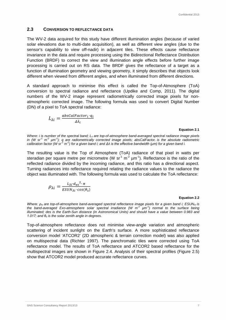
A standard approach to minimise this effect is called the Top-of-Atmosphere (ToA) conversion to spectral radiance and reflectance (Updike and Comp, 2011). The digital numbers of the WV-2 image represent radiometrically corrected image pixels for non-atmospheric corrected image. The following formula was used to convert Digital Number (DN) of a pixel to ToA spectral radiance:

𝐿𝜆𝑖 = 𝑎𝑏𝑠𝐶𝑎𝑙𝐹𝑎𝑐𝑡𝑜𝑟𝑖 ∙𝑞𝑖𝛥𝜆𝑖

Equation 2.1

Where: i is number of the spectral band; Lλ are top-of-atmosphere band-averaged spectral radiance image pixels in (W sr-1 m-2 µm-1); q are radiometrically corrected image pixels; absCalFactori is the absolute radiometric calibration factor (W sr-1 m-2) for a given band i; and Δλ is the effective bandwidth (µm) for a given band i.

The resulting value is the Top of Atmosphere (ToA) radiance of that pixel in watts per steradian per square metre per micrometre (W sr-1 m-2 µm-1). Reflectance is the ratio of the reflected radiance divided by the incoming radiance, and this ratio has a directional aspect. Turning radiances into reflectance required relating the radiance values to the radiance the object was illuminated with. The following formula was used to calculate the ToA reflectance:

𝜌𝜆𝑖 = 𝐿𝜆𝑖∙𝑑𝑒𝑠2∙ 𝜋𝐸𝑆𝑈𝑁𝜆𝑖 ∙𝑐𝑜𝑠(𝜃𝑠)

Equation 2.2

Where: ρλi are top-of-atmosphere band-averaged spectral reflectance image pixels for a given band i; ESUNλi is the band-averaged Exo-atmosphere solar spectral irradiance (W m-2 µm-1) normal to the surface being illuminated; des is the Earth-Sun distance (in Astronomical Units) and should have a value between 0.983 and 1.017; and θs is the solar zenith angle in degrees.

Top-of-atmosphere reflectance does not minimise view-angle variation and atmospheric scattering of incident sunlight on the Earth’s surface. A more sophisticated reflectance conversion model ‘ATCOR2’ (2D atmospheric & terrain correction model) was also applied on multispectral data (Richter 1997). The panchromatic tiles were corrected using ToA reflectance model. The results of ToA reflectance and ATCOR2 based reflectance for the multispectral images are shown in Figure 2.4. Analysis of their spectral profiles (Figure 2.5) show that ATCOR2 model produced accurate reflectance curves.

Confidential 2013


Figure 2.4 DN to Reflectance conversion results shown using same contrast stretch algorithm; (a) origanl image, (b) ToA reflectance and (c) ATCOR2 model based reflectnace.

Figure 2.5 Spectral response curve of different features; (a) DN response, (b) ToA reflectance and (c) ATCOR2 based reflectance.

Further analysis was performed by calculating the most widely used vegetation indices, referred to as the Normalized Difference Vegetation Index (NDVI), and based on the following equation:

NDVI = �ρλNIR − ρλRED��ρλNIR + ρλRED�

Equation 2.3

Where: ρλ are band-averaged spectral reflectance image pixels for a given band.

The differential reflection in the red (R) and near-infrared (NIR) bands enables monitoring of the density and intensity of green vegetation growth using the spectral reflectivity of solar radiation. Green leaves commonly show better reflection in the near-infrared wavelength range than in visible wavelength ranges (Rouse et al., 1973). When leaves are water stressed, diseased, or dead, they become more yellow thus reflect more in the red band while reflect significantly less in the near-infrared range. Clouds, water, and snow show

Confidential 2013


better reflection in the visible range than in the near-infrared range, while the difference approximates zero for rock and bare soil.

The NDVI process creates a single-band dataset whose values range between -1 to +1. The NDVI for the radiometrically corrected (unprocessed), top-of-atmosphere reflectance and ATCOR2 based reflectance images are shown in the Figure 2.6 below. These images are colour coded in different shades of blue, cyan, green, yellow, and red. The negative values in shades of blue to cyan represent water, moist sand and hill shaded soil. The values near zero appear as shades of green represent bare or exposed soil while positive values appear as shades of yellow to red mainly represent greenery. The ATCOR2 model reflectance data produced correct NDVI values for the shaded and sunlit parts of the images and was used for further processing.

Figure 2.6 Colour coded display of NDVI results for (a) unprocessed, (b) ToA reflectance, and (c) ATCOR2 reflectance images. Blue to cyan tone represents water, moist soil and shaded areas; green is bare or exposed soil; yellow to red tones indicate vegetated areas; note the changes between the images for shaded (solid arrow) and sunlit areas (dashed arrow).

2.4 MOSAICKING AND IMAGE FUSION

The next process was to generate a seamless and colour balanced mosaic from atmospherically corrected multispectral and panchromatic data tiles. Figure 2.7 shows the mosaics and their cutlines. Since the panchromatic tiles are corrected to ToA reflectance only, the mosaic shows a dark hue of grey tone along the margin of central and western tiles because no correction was applied to adjust different viewing angles between these two tiles. This appears strongly at small scales, e.g. 1:25 000, but diffuses when data is displayed at large scales, e.g. 1:5 000 (see Figure 2.8).

Confidential 2013


Figure 2.7 Colour balanced mosaic of multispectral and panchromatic data tiles with the seamline boundary, cutlines are shown as blue lines.

Figure 2.8 A mosaic of panchromatic image shows a dark hue of grey along the western tile at 1:25,000 scale (left); it shows a seamless joinery of tiles on large scales below 1:5,000(right), cutlines are shown as blue lines.

A ToA reflectance corrected panchromatic mosaic is then injected into a multispectral mosaic to generate a high resolution multispectral image. This process is called image fusion or panchromatic sharpening. Two image fusion processes were applied to these mosaics, which show significant improvement in visualising landslides and other high frequency structures such as urban features. A hyperspherical colour space (HCS) resolution merge technique (Padwick et al., 2010), devised by DigitalGloble, to pan-sharpen 8-band WV-2 data, has been tested along with the contrast and luminance normalised (CLN) fusion method (Ashraf et al., 2013). A CLN fusion method, developed by the University of Waikato (NZ) minimises spectral reflectance distortions in high-wavelength data channnels such as Red Edge and Near Infra-red. The results from these image fusion methods are displayed in Figure 2.9.

Confidential 2013


Figure 2.9 (a) WorldView-2 multispectral image at Cable Bay showing bands 5, 3, 2 as Red, Green, Blue; (b) WV-2 panchromatic image of the same extent; (c) CLN based pan-sharpened image; and (d) HCS pan-sharpened multispectral image.

Figure 2.10 displays spectral profiles along the yellow line (as shown in Figure 2.9) for the panchromatic as well as red, red-edge and NIR1 bands of the multispectral (2 m resolution) and pan-sharpened multispectral (0.5 m resolution) images. Since these high-wavelength bands are salient toward spectral classification, the result is less spectral distortion during the CLN fusion process compared to HCS. Therefore, CLN fused multispectral mosaic was used for further classification to delimit landslides. A digital copy of the resulting corrected satellite image for the NCC territorial boundary is avalaible in GeoJPEG2000 format (*.jp2) in the disk at the back of this report.

Confidential 2013


Figure 2.10 Spectral profiles of (a) the NIR1 band, (b) the red-edge band, and (c) the red band of multispectral (MS) image (green line), CLN based pan-sharpened image (red line) and HCS pan-sharpened image (blue line). The spectral profile of panchromatic band appears as black dashed line.

Confidential 2013


2.5 SPECTRAL CLASSIFICATION

In the next step, spectral classification was performed to delimit landslides. The Spectral Angle Mapper (SAM) based classification tool within Intergraph/ERDAS Imagine was used to conduct supervised classification. SAM is a physically-based spectral classification that uses an n-dimensional angle to match pixels to reference spectra (Kruse et al., 1993). When used on calibrated reflectance data, this technique is relatively insensitive to illumination and albedo effects.

SAM classification was tested on the original, ToA reflectance and ATCOR2 reflectance sub-images to compare its classification effectiveness on different processed datasets (along yellow line in Figure 2.9). Preliminary results show that ATCOR2 data produced better demarcation of landslide boundaries. Figure 2.11 shows that there is an over representation of grass pixels classed as landslides (shown as red color) in the orginal data compared to the classification of ATCOR2 based reflectance image.

Figure 2.11 SAM classification results on the unprocessed (middle) and ATCOR2 reflectance (right) images. Red shades represent landslides, green and yellow shades represent grass and scrub landuse

The SAM relies solely on the spectral response of individual pixels for classification. End-member spectra (or the training sample data) used by SAM were extracted directly from the image from hand digitized polygons of features of interest, e.g. bare ground, pasture, forestry, urban, cloud etc. Using the reflectance of different training samples, the pan-sharpened mosaic was classed into different categories. An example of the bareground categories are overlaid on a mosaic as shades of red and yellow respectively in Figure 2.12.

Higher reflectance due to haze and presence of thin cloud over certain parts resulted in many of these areas being incorrectly classified. Reflectance from unmetalled hill tracks, rock outcrops, eroding cliffs along the coastline were occasionally identified within the landslide classes. These unwanted classes were manually cleaned from the data, then converted into ESRI Shapefile format. Due to partial revegetation of some landslides, some single features were mapped as multiple polygons. To address this, a boundary filter of 1 m (equivalent to 4 pixels between features) was applied to the dataset, to group all polygons within this extent. It was assumed that polygons within this filter distance represented a single landslide.

Confidential 2013


Figure 2.12 (a – c) represents a section of imagery where haze is absent. (e – f) represents a section of imagery where haze is present. The red shading represents classification of landslides, note the over classification in the lower right hand corner of (e) and (f). The yellow outline represents the final landslide classification after manual editing.

Confidential 2013


3.0 RESULTS

The total area and other statistics of multiple landslides classified from the WV-2 image within the NCC territorial boundary are summarised in Table 3.1. A digital copy of this data is avalaible as an ESRI Shapefile in the disk at the back of this report.

Table 3.1 Statistics of landslide classification of the WorldView-2 mosaic within Nelson City Council boundary.

Landslide Statistics

Number of landslides 1519 polygons

Minimum size 1 m2

Maximum size 7380.25 m2

Average size 169.94 m2

Median (landslide occurrences) 49.0 m2

Median (landslide surface area) 576 m2

Std. Deviation 422.32 m2

Total Area 258138.23 m2

Distribution of landslides based on their surface area is shown in Figure 3.1, the spatial distribution is shown in Figure 3.2.

Figure 3.1 Surface area distribution of landslide occurences in the Nelson area, most landslides are less than 250 m2 and are shallow failures.

Confidential 2013


Figure 3.2 Distribution of landslides in Nelson area.

Confidential 2013


3.1 DIFFERENTIATING BETWEEN SCAR AND DEBRIS TRAIL

While the high resolution of the WV-2 imagery renders it likely to distingush between erosion forms (gully/landslide) and landslide components (scar evacuation/debris tail) during the primary classification, this approach was outside the scope of this project’s proposal, and has not been undertaken.

3.2 ACCURACY ASSESSMENT

Validation of the remotely sensed imagery results was achieved through the comparison of the SAM classification with visual assessment by expert users. A stratified random approach was adopted where points were randomly distributed across the region, with 100 points constrained to areas classified as bare ground, and another 100 points constrained to areas of non-bare ground. The classification of these points was extracted from the raster classification layer and each point was visually assessed against the imagery and marked as either correct or incorrect. These results were then compared within a confusion matrix to derive the degree of commission and omission in the classification (Table 3.2). Errors of commission result when a point is incorrectly associated with another classification e.g. the point is classified as bare ground but is located on a pasture covered stable slope. Errors of omission occur when a point is not identified as representing bare ground but should have been identified as belonging to this particular class. Mapping accuracy for each class is the number of correctly identified pixels within the displayed area, divided by that number plus error pixels of commission and omission. The overall mapping accuracy was 82.6 %

Table 3.2 Bare ground classification accuracy assessment.

Classification Omissions Commissions Accuracy

Landslide bare ground (18/100)

18%

(1/100)

1 %

82/(82+1+18)

81.2 %

Non-landslide bare ground (1/100)

1%

(18/100)

18 %

99/(99+1+18)

83.9 %

3.3 LIMITATIONS OF SATELLITE IMAGERY

There were the following limitations in acqusition and processing of this WV-2 dataset which restricted the ability to utilise this data to its fullest.

The first and the foremost criticial limitation was the length of time between the landslide events and the date of data acqusition. This lag time was more than seven months for the WV-2 imagery. During this time there were few windows of fine weather and the satellite was either not positioned adequately during orbit, or did not have sufficent data storage space to collect the required data. As compared to satellite data, acqusition of aerial images is more practical and can be planned and initiated with better knowledge of local weather conditions.

An advantage of capturing high multispectral high resolution (8-band) images using WV-2 data was one of the reasons to test it for accurate detection and mapping of landslides. Delayed acquisition from the event date meant that the event clean up had already taken place in urban areas and may have led to vegetation regeneration in landslide areas so that reduced the contrast between exposed bare ground and other bare ground features (such as tracks and logged forest land). Acquisition of aerial images in early January 2012 (as organised by the Tasman District Council) depicts a better sanpshot of near-real-time

Confidential 2013


damage. Although such data was delivered to the council as 3-band visible coloured image, actual data was captured in four bands of visible to near infra-red spectrum. This could be considered better in terms of spatial resolutions and sufficent in terms of spectral resolution. The use of the additional NIR band could be more cost-effective than requesting a new satellite image with a 6 month tasking window.

The month of June is a winter solstice for the Southern hemisphere. The 21st June is the date when sun is at its lowest altitude above the horizon. A delay in data acquisition led to the imagery being acquired around this time. The topography of Nelson city and the surrounding region varies from sea level to aproximately 500 m above mean sea level. In this case, a low solar elevation causes significant topographic shadowing that leads to a high contrast image. The conversion of the data from digital number to reflectance using the ATCOR2 model helped by compensating the spectral response of similar features in shade and sunlit regions so that image ratios (such as the NDVI) could produce consistent results. However, more sophisticated topographic correction models such as ATCOR3 (3D atmospheric and terrain correction) and use of a digital elevation model (DEM) of the area to simulate topographic shade and sunlit regions, alleviates the reflectance of features in shaded regions and improves image quality for further processing. Testing of such topographic correction methods would require more processing time.

Another limitation was the prevalence of cloud and hazy atmospheric conditions in various parts of the image. Although ATCOR2 model could compensate for haze correction, initial haze correction results were unimpressive due to the high contrast between shaded and sunlit regions. A combination of haze and topographic correction could be more useful but as mentioned above, the benefit is reduced when data quality is less than ideal and represents changes in the ground conditions up to eight months after the event.

Confidential 2013


4.0 ACKNOWLEDGEMENT

The funding for this report was provided through Envirolink grant NLCC 63, courtesy of Paul Sheldon, Environmental Monitoring Co-ordinator, Nelson City Council.

The authors would like to acknowledge Jon Carey and Julie Lee (GNS Science) for reviewing this report, and Sally Dellow (GNS Science) for discussions about the Nelson/Tasman 2011 flood event.

5.0 REFERENCES

Ashraf, S., Brabyn, L. and Hicks, B. J. 2013. Introducing Contrast and Luminance Normalisation to improve the quality of subtractive resolution merge technique. International Journal of Image and Data Fusion, Paper under review.

Dellow, S., 2013. Personal communication. GNS Science, Lower Hutt, New Zealand.

ICNZ, 2012. Insurance Council of New Zealand; http://www.icnz.org.nz/current/weather/index.php [online]. [Accessed 24 Jan. 2013].

Kruse, F., Lefkoff, A.B., Boardman, J.W., Heidebrecht, K.B., Shapiro, A.T., Barloon, P.J., and Goetz, A.F.H., 1993. The Spectral Image Processing System (SIPS) – Interactive Visualization and Analysis of Imaging Spectrometer Data. Remote Sensing of Environment, 44 (2-3), pp. 145-163.

Nelson Tasman Civil Defence, 2011. Nelson Tasman Emergency Management Group News; Heavy rain updates; http://nelsontasmancivildefence.co.nz/heavy-rain-update-12 [online]. [Accessed 18 Jan. 2013].

NIWA, 2013. NZ Historic Weather Events Catalog; http://hwe.niwa.co.nz [online]. [Accessed 18 Jan. 2013].

Padwick, C., Deskevich, M., Pacifici, F. and Smallwood, S., 2010. WorldView-2 Pan-Sharpening. ASPRS 2010 Annual Conference: Opportunities for Emerging Geospatial Technologies. San Diego, California: ASPRS.

Richter, R. 1997. Correction of atmospheric and topographic effects for high spatial resolution satellite imagery. International Journal of Remote Sensing, 18(5), 1099-1111.

Rouse, J.W., Haas, R.H., Schell, J.A. and Deering, D.W., 1973. Monitoring vegetation systems in the Great Plains with ERTS. In 3rd ERTS Symposium, NASA SP-351 I, pp. 309–317.

Updike, T. and Comp, C., 2011. Radiometric Use of WorldView-2 Imagery. Longmont, Colorado: DigitalGlobe, Inc. [Accessed 5 Oct 2012; https://www.digitalglobe.com/downloads/Radiometric_Use_of_WorldView-2_Imagery.pdf.

http://www.icnz.org.nz/current/weather/index.php

http://nelsontasmancivildefence.co.nz/heavy-rain-update-12

http://hwe.niwa.co.nz/

https://www.digitalglobe.com/downloads/Radiometric_Use_of_WorldView-2_Imagery.pdf

1 Fairway Drive

Avalon

PO Box 30368

Lower Hutt

New Zealand

T +64-4-570 1444

F +64-4-570 4600

Dunedin Research Centre

764 Cumberland Street

Private Bag 1930

Dunedin

New Zealand

T +64-3-477 4050

F +64-3-477 5232

Wairakei Research Centre

114 Karetoto Road

Wairakei

Private Bag 2000, Taupo

New Zealand

T +64-7-374 8211

F +64-7-374 8199

National Isotope Centre

30 Gracefield Road

PO Box 31312

Lower Hutt

New Zealand

T +64-4-570 1444

F +64-4-570 4657

Principal Location

www.gns.cri.nz

Other Locations

processing and classifying satellite imagery to in the nelson area … · 2017-01-19 · processing...

Documents