Processing of large document collections

Part 2 (Text categorization, term selection)

Helena Ahonen-Myka

Spring 2005

2

Text categorization, continues

• problem setting

• machine learning approach

• example of a learner: Rocchio method

• term selection (for text categorization)

3

Text categorization: problem setting

• let – D: a collection of documents

– C = {c1, …, c|C|} : a set of predefined categories

– T = true, F = false

• the task is to approximate the unknown target function ’: D x C -> {T,F} by means of a function : D x C -> {T,F}, such that the functions ”coincide as much as possible”

• function ’ : how documents should be classified

• function : classifier (hypothesis, model…)

4

Some assumptions

• categories are just symbolic labels– no additional knowledge of their meaning is

available

• no knowledge outside of the documents is available– all decisions have to be made on the basis

of the knowledge extracted from the documents

– metadata, e.g., publication date, document type, source etc. is not used

5

Some assumptions

• methods do not depend on any application-dependent knowledge– but: in operational (”real life”) applications

all kind of knowledge can be used (e.g. in spam filtering)

• note: content-based decisions are necessarily subjective– it is often difficult to measure the

effectiveness of the classifiers– even human classifiers do not always agree

6

Single-label, multi-label TC

• single-label text categorization– exactly 1 category must be assigned to

each dj D

• multi-label text categorization– any number of categories may be assigned

to the same dj D

7

Single-label, multi-label TC

• special case of single-label: binary

– each dj must be assigned either to category ci or to its complement ¬ ci

• the binary case (and, hence, the single-label case) is more general than the multi-label– an algorithm for binary classification can

also be used for multi-label classification– the converse is not true

8

Single-label, multi-label TC

• in the following, we will use the binary case only:– classification under a set of categories C =

set of |C| independent problems of classifying the documents in D under a given category ci, for i = 1, ..., |C|

9

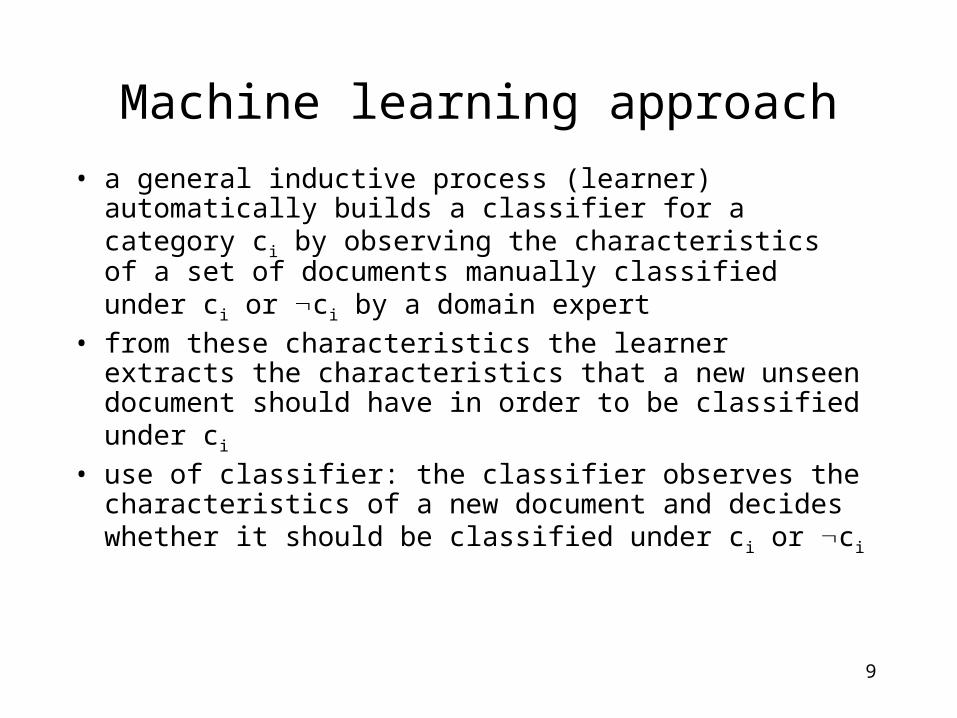
Machine learning approach

• a general inductive process (learner) automatically builds a classifier for a category ci by observing the characteristics of a set of documents manually classified under ci or ci by a domain expert

• from these characteristics the learner extracts the characteristics that a new unseen document should have in order to be classified under ci

• use of classifier: the classifier observes the characteristics of a new document and decides whether it should be classified under ci or ci

10

Classification process: classifier construction

Learner

ClassifierDoc 1; Label: yesDoc2; Label: no

...Docn; Label: yes

Training set

11

Classification process: testing the classifier

Test set Classifier

12

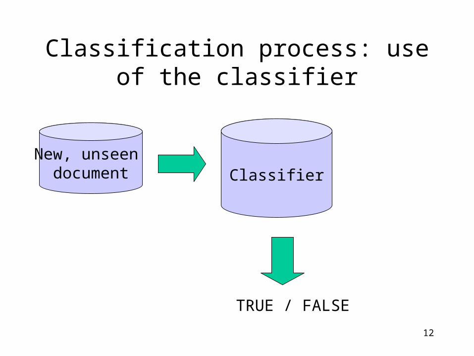
Classification process: use of the classifier

ClassifierNew, unseen

document

TRUE / FALSE

13

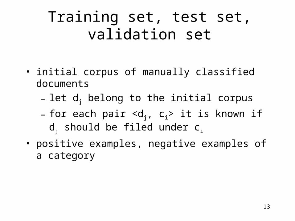
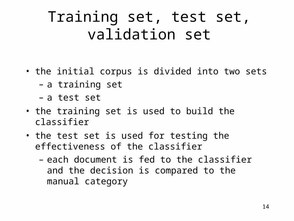
Training set, test set, validation set

• initial corpus of manually classified documents

– let dj belong to the initial corpus

– for each pair <dj, ci> it is known if dj should be filed under ci

• positive examples, negative examples of a category

14

Training set, test set, validation set

• the initial corpus is divided into two sets– a training set– a test set

• the training set is used to build the classifier

• the test set is used for testing the effectiveness of the classifier– each document is fed to the classifier and

the decision is compared to the manual category

15

Training set, test set, validation set

• the documents in the test set are not used in the construction of the classifier

• alternative: k-fold cross-validation– k different classifiers are built by

partitioning the initial corpus into k disjoint sets and then iteratively applying the train-and-test approach on pairs, where k-1 sets construct a training set and 1 set is used as a test set

– individual results are then averaged

16

Training set, test set, validation set

• training set can be split to two parts

• one part is used for optimising parameters– test which values of parameters yield the

best effectiveness

• test set and validation set must be kept separate

17

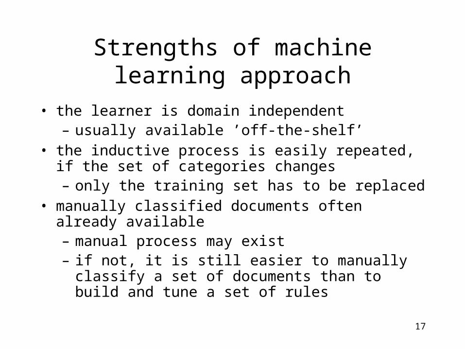
Strengths of machine learning approach

• the learner is domain independent– usually available ’off-the-shelf’

• the inductive process is easily repeated, if the set of categories changes– only the training set has to be replaced

• manually classified documents often already available– manual process may exist– if not, it is still easier to manually classify a

set of documents than to build and tune a set of rules

18

Examples of learners• Rocchio method• probabilistic classifiers (Naïve Bayes)• decision tree classifiers• decision rule classifiers• regression methods• on-line methods• neural networks• example-based classifiers (k-NN)• boosting methods• support vector machines

19

Rocchio method

• learner

• for each category, an explicit profile (or prototypical document) is constructed from the documents in the training set– the same representation as for the

documents– benefit: profile is understandable even for

humans

20

Rocchio method

• a profile of a category is a vector of the same dimension as the documents– in our example: 118 terms

• categories medicine, energy, and environment are represented by vectors of 118 elements

– the weight of each element represents the importance of the respective term for the category

21

Rocchio method

• weight of the kth term of the category i:

• POSi: set of positive examples

– documents that are of category i

• NEGi: set of negative examples

}{}{ |||| ijij NEGd i

kj

POSd i

kjki

NEG

w

POS

ww

22

Rocchio method

• in the formula, and are control parameters that are used to set the relative importance of positive and negative examples

• for instance, if =2 and =1, we don’t want the negative examples to have as strong influence as the positive examples

23

Rocchio method

• in our sample dataset: what is the weight of term ’nuclear’ in the category ’medicine’?

– POSmedicine contains the documents Doc1-Doc4, and NEGmedicine contains the documents Doc5-Doc10

• | POSmedicine | = 4 and |NEGmedicine| = 6

24

Rocchio method

– the weights of term ´nuclear´ in documents in POSmedicine

• w_nuclear_doc1 = 0.5

• w_nuclear_doc2 = 0

• w_nuclear_doc3 = 0

• w_nuclear_doc4 = 0.5

– and in documents in NEGmedicine

• w_nuclear_doc6 = 0.5

25

Rocchio method

• weight of ’nuclear’ in the category ’medicine’:– w_nuclear_medicine = 2*

(0.5 + 0.5)/4 – 1 * 0.5/6 = 0.5 - 0.08 = 0.42

26

Rocchio method

• using the classifier: cosine similarity of the category vector and the document vector is computed– |T| is the number of terms

||

1

2||

1

2

||

1),(T

k kj

T

k ki

T

k kjkiji

ww

wwdcS

27

Rocchio method

• the cosine similarity function returns a value between 0 and 1

• a threshold is given– if the value is higher than the threshold ->

true (the document belongs to the category)

– otherwise -> false (the document does not belong to the category)

28

Strengths of Rocchio method

• simple to implement

• fast to train

• search engines can be used to run a classifier

29

Weaknesses of Rocchio method

• if the documents in a category occur in disjoint clusters, a classifier may miss most of them– e.g. two types of Sports news: boxing and

rock-climbing– the centroid of these clusters may fall

outside all of these clusters

30

_

_

_

+++

+ ++

++

++

_

_ _

_ __

_

_

_

__

_ _

31

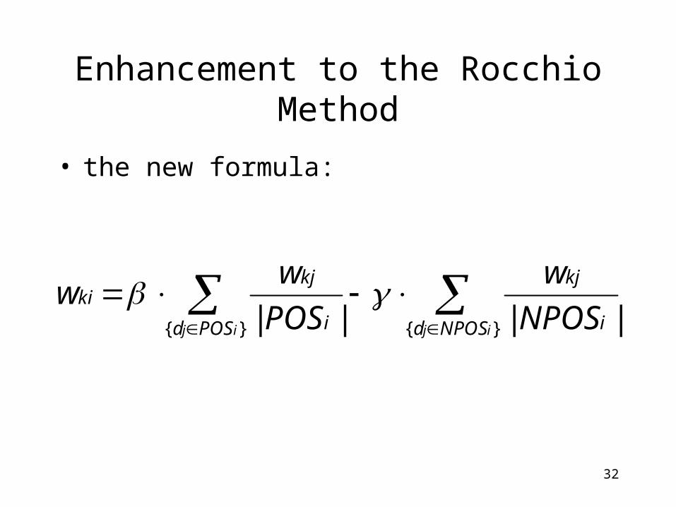
Enhancement to the Rocchio Method

• instead of considering the set of negative examples in its entirety, a smaller sample can be used– for instance, the set of near-positive

examples

• near-positives (NPOSc): the most positive amongst the negative training examples

32

Enhancement to the Rocchio Method

• the new formula:

}{}{ |||| ijij NPOSd i

kj

POSd i

kjki

NPOS

w

POS

ww

33

Enhancement to the Rocchio Method

• the use of near-positives is motivated, as they are the most difficult documents to distinguish from the positive documents

• near-positives can be found, e.g., by querying the set of negative examples with the centroid of the positive examples– the top documents retrieved are most similar

to this centroid, and therefore near-positives• with this and other enhancements, the

performance of Rocchio is comparable to the best methods

34

Term selection

• a large document collection may contain millions of words -> document vectors would contain millions of dimensions– many algorithms cannot handle high

dimensionality of the term space (= large number of terms)

– very specific terms may lead to overfitting: the classifier can classify the documents in the training data well but fails often with unseen documents

35

Term selection

• usually only a part of terms is used

• how to select terms that are used?– term selection (often called feature

selection or dimensionality reduction) methods

36

Term selection

• goal: select terms that yield the highest effectiveness in the given application

• wrapper approach– the reduced set of terms is found iteratively

and tested with the application

• filtering approach– keep the terms that receive the highest

score according to a function that measures the ”importance” of the term for the task

37

Term selection

• many functions available– document frequency: keep the high

frequency terms• stopwords have been already removed

• 50% of the words occur only once in the document collection

• e.g. remove all terms occurring in at most 3 documents

38

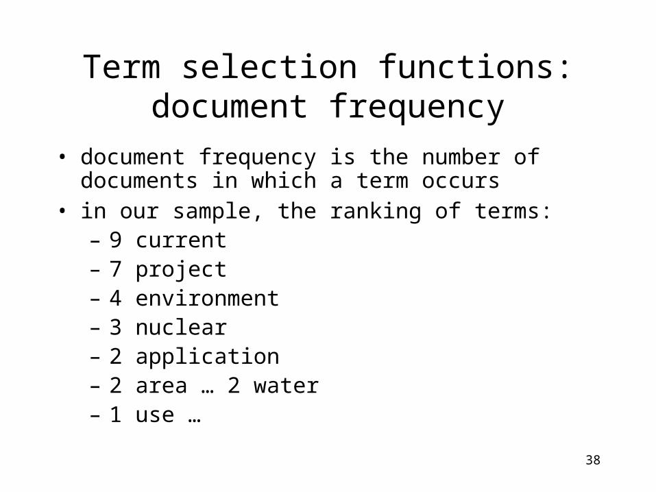
Term selection functions: document frequency

• document frequency is the number of documents in which a term occurs

• in our sample, the ranking of terms:– 9 current– 7 project– 4 environment– 3 nuclear– 2 application– 2 area … 2 water– 1 use …

39

Term selection functions: document frequency

• we might now set the threshold to 2 and remove all the words that occur only once

• result: 29 words of 118 words (~25%) selected

40

Term selection: other functions

• Information-theoretic term selection functions, e.g.– chi-square– information gain– mutual information– odds ratio– relevancy score

41

Term selection: information gain

• Information gain: measures the (number of bits of) information obtained for category prediction by knowing the presence or absence of a term in a document

• information gain is calculated for each term and the best n terms are selected

42

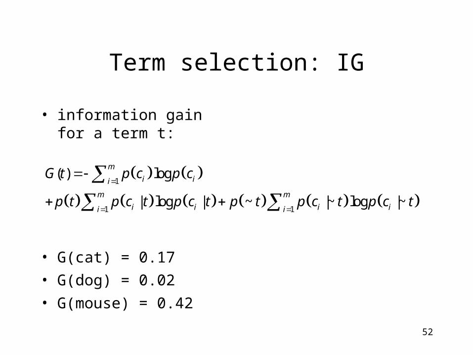
Term selection: IG

• information gain for term t:– m: the number of categories

1

1

1

( ) log

| log |

~ |~ log |~

m

i ii

m

i ii

m

i ii

G t p c p c

p t p c t p c t

p t p c t p c t

43

Estimating probabilities

• Doc 1: cat cat cat (c)

• Doc 2: cat cat cat dog (c)

• Doc 3: cat dog mouse (~c)

• Doc 4: cat cat cat dog dog dog (~c)

• Doc 5: mouse (~c)

• 2 classes: c and ~c

44

Term selection: estimating probabilities

• P(t): probability of a term t– P(cat) = 4/5, or

• ‘cat’ occurs in 4 docs of 5

– P(cat) = 10/17 • the proportion of the occurrences of ´cat’ of the

all term occurrences

45

Term selection: estimating probabilities

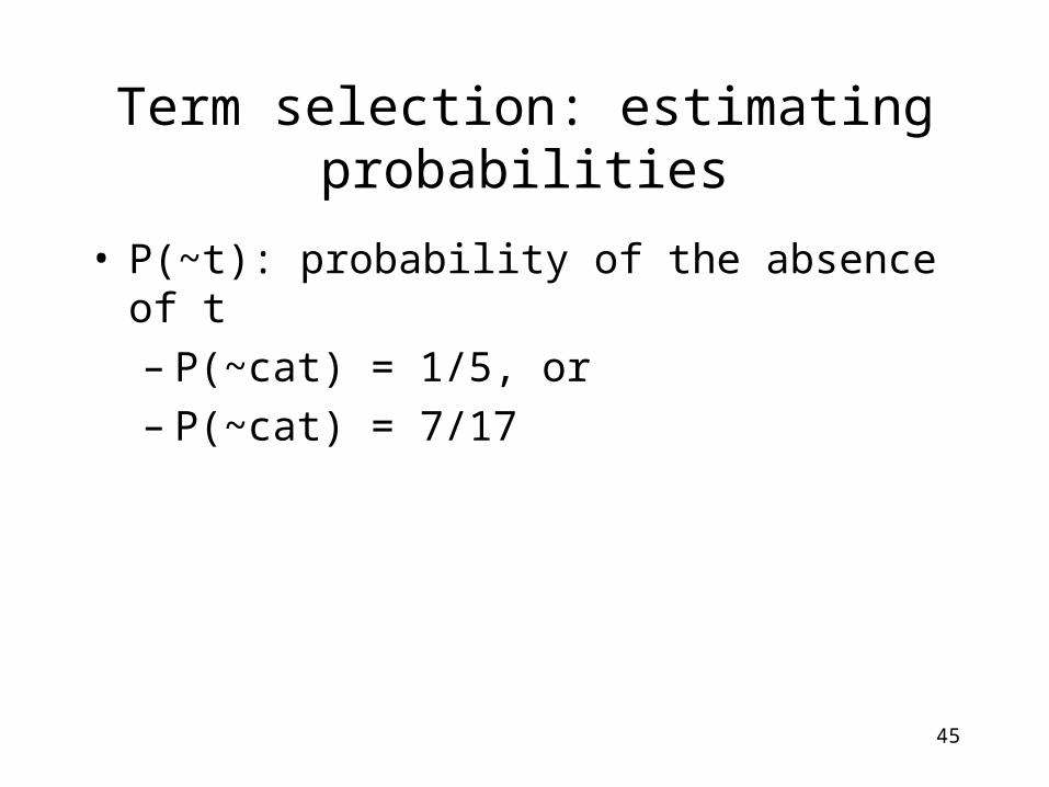
• P(~t): probability of the absence of t– P(~cat) = 1/5, or– P(~cat) = 7/17

46

Term selection: estimating probabilities

• P(ci): probability of category i

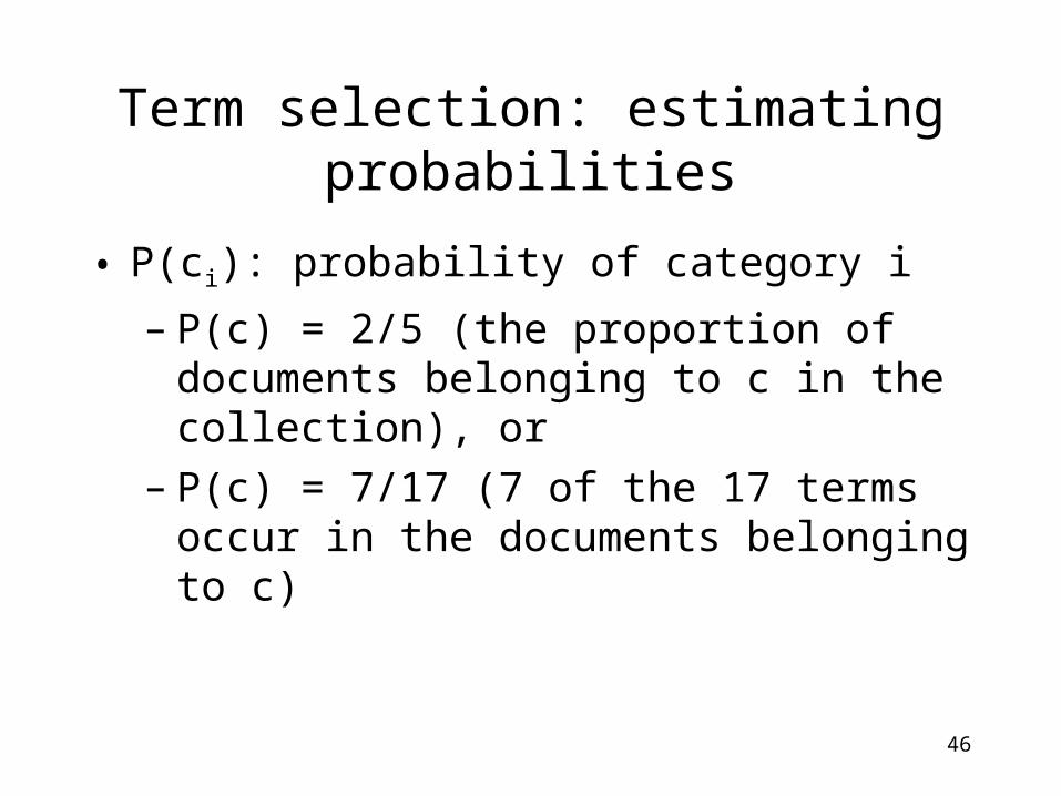
– P(c) = 2/5 (the proportion of documents belonging to c in the collection), or

– P(c) = 7/17 (7 of the 17 terms occur in the documents belonging to c)

47

Term selection: estimating probabilities

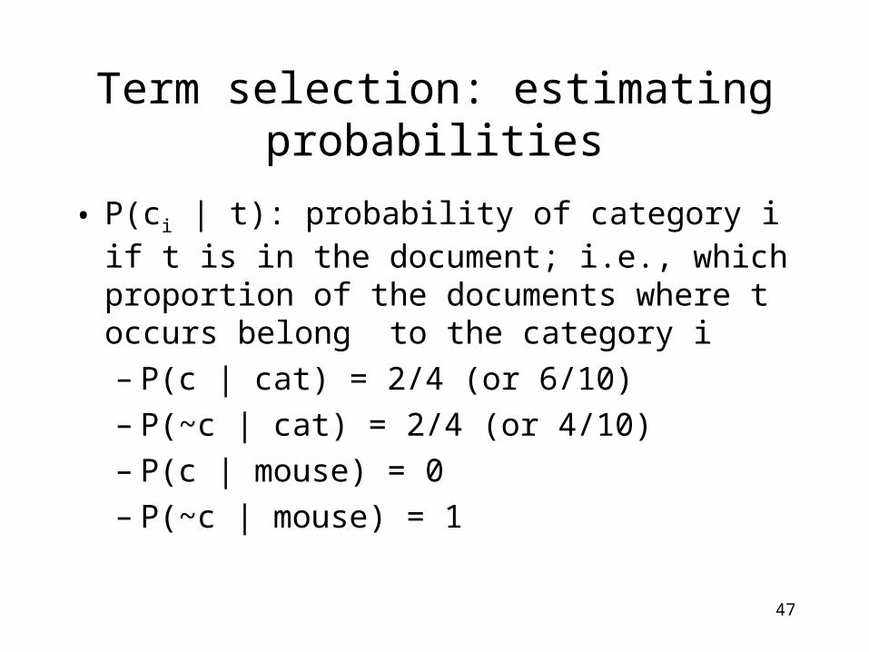
• P(ci | t): probability of category i if t is in the document; i.e., which proportion of the documents where t occurs belong to the category i– P(c | cat) = 2/4 (or 6/10)– P(~c | cat) = 2/4 (or 4/10)– P(c | mouse) = 0– P(~c | mouse) = 1

48

Term selection: estimating probabilities

• P(ci | ~t): probability of category i if t is not in the document; i.e., which proportion of the documents where t does not occur belongs to the category i– P(c | ~cat) = 0 (or 1/7)– P(c | ~dog) = ½ (or 6/12)– P(c | ~mouse) = 2/3 (or 7/15)

49

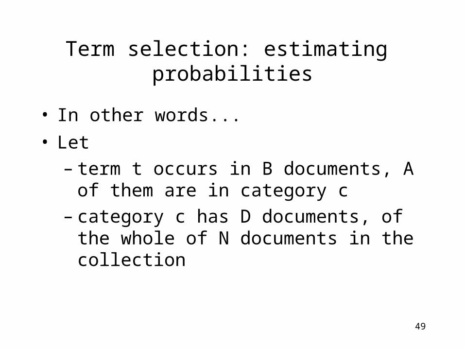
Term selection: estimating probabilities

• In other words...

• Let– term t occurs in B documents, A of

them are in category c– category c has D documents, of the

whole of N documents in the collection

50

Term selection: estimating probabilities

cdocs

containing t

N documents

B documents

A documents

D documents

51

Term selection: estimating probabilities

• For instance,– P(t): B/N– P(~t): (N-B)/N– P(c): D/N– P(c|t): A/B– P(c|~t): (D-A)/(N-B)

52

Term selection: IG

• information gain for a term t:

• G(cat) = 0.17

• G(dog) = 0.02

• G(mouse) = 0.42

1

1 1

( ) log

| log | ~ |~ log |~

m

i ii

m m

i i i ii i

G t p c p c

p t p c t p c t p t p c t p c t