PRODUCT DEVELOPMENT MEETS INSTRUCTIONAL DESIGN- A CASE STUDY IN

THE REDESIGN OF A FUNDAMENTALS OF FLUIDS COURSE

by

David Andrew Torick

Bachelor of Science, GMI Engineering & Management Institute, 1996

Master of Education, The Ohio State University, 2000

Submitted to the Graduate Faculty of

Swanson School of Engineering in partial fulfillment

of the requirements for the degree of

Master of Science

University of Pittsburgh

2009

ii

UNIVERSITY OF PITTSBURGH

SWANSON SCHOOL OF ENGINEERING

This thesis was presented

by

David Torick

It was defended on

April 1, 2009

and approved by

Dr. Daniel Budny, Associate Professor, Civil and Environmental Engineering

Dr. Leonard Casson, Associate Professor, Civil and Environmental Engineering

Dr. Amir Koubaa, Associate Professor, Civil and Environmental Engineering

Thesis Advisor: Dr. Daniel Budny, Associate Professor, Civil and Environmental Engineering

iii

Copyright © by David Torick

2009

iv

Over the past two years, substantial research and implementation efforts have occurred to

support the mobilization of the laboratory experiences in the Fundamental of Fluids course. No

longer does the laboratory component of this course require substantial year-long floor space.

The entire laboratory curriculum has been redesigned to use equipment designed and fabricate

in-house. This equipment is able to be stored in a closet and easily setup and utilized in a just-in-

time fashion. The actual laboratory experiences and corresponding procedures and documents

have been modified and improved based off of research in engineering education and student

feedback. This thesis describes the method of applying a product development approach to

instructional design. It also contains the curriculum, assessment methods, and results of

implementing the new curriculum.

PRODUCT DEVELOPMENT MEETS INSTRUCTIONAL DESIGN- A CASE STUDY

IN THE REDESIGN OF A FUNDAMENTALS OF FLUIDS COURSE

David Torick, M.S.

University of Pittsburgh, 2009

v

TABLE OF CONTENTS

ACKNOWLEDGEMENTS ........................................................................................................ X

1.0 INTRODUCTION ........................................................................................................ 1

2.0 OVERVIEW OF EDUCATIONAL RESEARCH .................................................... 3

2.1 EDUCATIONAL DESIGN ................................................................................. 4

2.1.1 Influences of Product Development ............................................................... 4

2.1.2 Idea Generation ............................................................................................... 6

2.2 RELEVANT TRENDS IN EDCUATION ......................................................... 7

2.2.1 Real-World Context ........................................................................................ 8

2.2.2 Contributions to the Preparation of Engineers ............................................ 9

2.2.3 Opportunities for Practice ............................................................................ 10

2.3 BEST PRACTICES IN LABORATORY EXPERIENCES .......................... 11

2.4 ASSESSMENT OF STUDENT KNOWLEDGE ............................................ 13

2.4.1 Assessment Approaches ................................................................................ 14

2.4.2 Data Analysis Approaches ............................................................................ 15

3.0 DEVELOPING NEW LABORATORY EXPERIENCES ..................................... 18

3.1 PROCESS OVERVIEW ................................................................................... 18

3.1.1 Determination of Design Constraints .......................................................... 19

3.1.2 Determination of Laboratory Curriculum .................................................. 22

vi

3.1.3 Development of Laboratory Equipment...................................................... 27

3.1.3.1 Utilizing Existing Equipment ............................................................. 27

3.1.3.2 Developing New Equipment ............................................................... 28

3.1.4 Development of Supporting Material .......................................................... 32

3.1.5 Pilot Study and Assessment .......................................................................... 35

3.1.5.1 Pilot Study ............................................................................................ 36

3.1.5.2 Assessment ........................................................................................... 37

3.1.6 Finalization of Lab Equipment and Curriculum........................................ 40

3.2 ITERATIONS IN THE DESIGN PROCESS.................................................. 41

4.0 NEWLY DESIGNED LABORATORY EXPERIENCES ...................................... 44

5.0 DATA ANALYSIS ..................................................................................................... 46

5.1 STATISTICAL ANALYSIS APPROACHES ................................................. 47

5.1.1 Effect Size ....................................................................................................... 48

5.1.2 Mann-Whitney U Test ................................................................................... 49

5.2 RESULTS AND DISCUSSION ........................................................................ 50

5.2.1 Self-Assessment Survey ................................................................................. 50

5.2.2 Evaluation Survey.......................................................................................... 52

5.2.3 Exam Data ...................................................................................................... 55

5.2.4 ABET Criterion ............................................................................................. 58

6.0 SUMMARY AND CONCLUSIONS ........................................................................ 65

7.0 FUTURE WORK ....................................................................................................... 69

APPENDIX A - TEACHING ASSISTANT MANUAL ........................................................... 72

APPENDIX B - LABORATORY EXPERIENCE HANDOUTS ........................................... 97

vii

APPENDIX C - CEE 1402 SPRING 2009 SYLLABUS ........................................................ 125

APPENDIX D - FUNDAMENTALS OF FLUIDS SELF-ASSESSMENT SURVEY ........ 128

APPENDIX E - SEMESTER EVALUATION FORM .......................................................... 130

BIBLIOGRAPHY ..................................................................................................................... 132

viii

LIST OF TABLES

Table 1. Design Constraints for the Redesign of the Fluids Laboratory Experiences .................. 21

Table 2. Over-Arching Principles for Laboratory Design ............................................................ 23

Table 3. Summary of Content Analysis for the Fundamentals of Fluids Course ......................... 25

Table 4. Content Areas Covered in Laboratory Experiences ....................................................... 26

Table 5. Laboratory Experiences and Device Types .................................................................... 29

Table 6. Pilot Study Schedule ....................................................................................................... 37

Table 7. Summary of Products for all of the New Laboratory Experiences ................................. 45

Table 8. Summary Table of Concepts with the Largest Difference in Percent of Gain Realized 47

Table 9. Significant Effect Size Results for the Self-Assessment Survey .................................... 51

Table 10. Mann- Whitney U Test Results for the Self-Assessment Survey ................................. 52

Table 11. Effect Size for Evaluation Survey ................................................................................ 53

Table 12. Mann-Whitney U test for the Evaluation Survey ......................................................... 54

Table 13. Project Constraints Analysis ......................................................................................... 66

ix

LIST OF FIGURES

Figure 1. Basic Stages in the Design Process ................................................................................. 5

Figure 2. Six Step Design Process .................................................................................................. 5

Figure 3. Sample Questions from the Mathematics Inventory Survey ......................................... 15

Figure 4. Design Process Utilized to Develop New Laboratory Experiences .............................. 19

Figure 5. Multi-Purpose Device 1 ................................................................................................. 30

Figure 6. Multi-Purpose Device 2 ................................................................................................. 31

Figure 7. Pooled Standard Deviation ............................................................................................ 48

Figure 8- Test 1 Results ................................................................................................................ 56

Figure 9- Test 2 Results ................................................................................................................ 57

Figure 10- Final Exam Results ..................................................................................................... 58

Figure 11- ABET Criterion 2 Outcome A Results ........................................................................ 60

Figure 12- ABET Criterion 2 Outcome B Results ........................................................................ 61

Figure 13- ABET Criterion 2 Outcome E Results ........................................................................ 62

Figure 14- ABET Criterion 2 Outcome E Results ........................................................................ 63

x

ACKNOWLEDGEMENTS

The support I have received through funding and guidance from several different sources made

this thesis possible. I want to thank the Civil and Environmental Engineering Department for the

financial support to pursue this research. I also need to acknowledge the funding from the

Mascaro Center for Sustainable Innovation in supplying funding while I pursued a brief

exploration into the emerging study of sustainability. The Freshman Engineering program also

provided financial assistance to develop key aspects of this thesis.

While at the university I have had several advisors as I have explored and attempted to

find a mutually beneficial relationship. I appreciate the time that each advisor has invested with

me and wish them all success and enjoyment in their pursuits. A special thanks to: Dr. Mike

Lovell, Dr. Amy Landis, and Dr. Joe Marriott. Although I did not complete thesis related

research with them, each has had an impact while I was at the university.

I appreciate the feedback and guidance from my thesis committee members, Dr. Amir

Koubaa and Dr. Leonard Casson. Their insights have strengthened the quality of this thesis and

have helped me more clearly communicate the work that was conducted. I would have liked to

have worked more with each of them over the last few years and look forward to future

collaborations as I pursue my next career only one building away.

I would like to thank my advisor Dr. Daniel Budny for all he has done over the last two

years. First of all, I am grateful for the opportunity to write a thesis that involves two of my

xi

favorite career interests, teaching and design. I have appreciated the frank discussions about

engineering, academia, and life in general. Finally, I look forward to future collaborations to

benefit both of our student groups. Dr. Budny’s concern and passion for student learning,

achievement, and well-being is admirable and inspirational.

Moving back to Pittsburgh three years ago has had so many benefits. I am so grateful to

be closer to my family and appreciate their support and understanding over the last few years as I

pursued the many dreams that have taken away time I would have liked to have spent with them.

Having a loving and supportive family has made all the difference over the years as I have

pursued various careers and dreams. Knowing that there is a wonderful place to fall back to, no

matter what, makes it so much easier to leap into the unknown to follow my dreams.

I want to thank my old and new friends for the good times, support, and assistance over

the last two years. Luckily we are placed on Earth with a family and the opportunity to make

friends, without them life will be much less enjoyable and much more difficult.

A final thank you to life itself: the lessons, experiences, people, and circumstances have

all contributed to the ability and desire to complete this thesis. As I move forward I would like to

reflect on a quote from Mark Twain, “Twenty years from now you will be more disappointed by

the things you didn’t do than by the ones you did do. So throw off the bowlines. Sail away from

the safe harbor. Catch the trade winds in your sails. Explore. Dream. Discover.”

1

1.0 INTRODUCTION

Benedum Hall, the home of most engineering departments at the University of Pittsburgh, is in

the middle of an extensive remodeling project. This project has caused the temporary loss of the

laboratory space for the Fundamental of Fluids course that is required of all Civil and

Environmental Engineering undergraduates. For a minimum of two semesters, the course’s lab

experiences will be taught in various locations throughout the building. The development of

portable experiences for students that can be stored in minimal space and easily setup each week

is required for the department to meet its educational requirements to the undergraduate students.

Additionally, over the last decade, ABET is directing universities to provide an engineering

education that is focused more on the process of learning than on the body of knowledge that

was typical before this decade [EAC, 2008]. Research at other universities shows that change in

the curriculum is challenging [Lamancusa, 2006]. The necessity of redesign has provided the

required resources to redesign the labs for portability and with an attention to 21st century

educational research and current ABET criteria.

The process of making these labs portable is not a trivial task. Other engineering

programs have reported that it is difficult to develop cheap and effective hands-on experiences to

enhance the engineering curriculum [Hesketh, 2000]. This thesis discusses the process of

redesigning these labs. The approach draws from best practices and experiences in product

2

development (PD) as well as information gathered from educational research and instructional

design (ID).

The emerging engineering education community is calling for increased rigor in research.

Early research showed a focus on curriculum improvements but lacked assessment [Borrego,

2007]. The overall objective of this thesis is curriculum improvement with rigor. This objective

is attained through three separate but related activities:

• curriculum development grounded in ID • curriculum design based on best-practices in engineering education • formative and summative feedback through several assessment methods

This thesis describes an approach to laboratory curriculum design that has shown to be beneficial

for increasing student understanding of fundamental of fluids topics. This approach has potential

to be used in other courses that require a redesign or updating of the laboratory experience.

3

2.0 OVERVIEW OF EDUCATIONAL RESEARCH

There is a vast resource of literature related to education research. Researchers and practitioners

in the fields of science, engineering, education, and psychology have been contributing to the

advancement of helping people learn for many years. This section will focus on four areas of

educational research that are necessary in the redesign of the laboratory experiences (LE). The

development of a systematic approach to curriculum design requires understanding of current

models of ID and curriculum development approaches. The need to examine trends in

engineering education and best practices in LE in engineering is also required. This process,

although necessary, can present significant problems in creating effective curriculum solutions. It

is cautioned, that the searching for ideas should be done at an abstract level [Schunn, 2008] to

limit the effects of design fixation [Smith, 1993] and allow for creative solutions to problems.

Finally, it is important to examine effective measures in assessment of student learning. There

are many approaches and available materials that can either be used or modified to match this

project’s goal. Combined, this overview was used to guide the development and assessment of

the new fluids laboratory curriculum.

4

2.1 EDUCATIONAL DESIGN

Effective product design is not the result of luck or intuition; it is a systematic approach to

providing a desired outcome. ABET criteria require that engineering programs provide courses

and opportunities for students to learn effective design principles and practice these skills [EAC,

2008]. There are also many journals that publish on the scholarship of design [Schunn, 2008]. It

is therefore rather shocking that little work has been done in the past to apply the engineering

approach of PD to ID [Rowland, 1993]. PD is an iterative process that has definitive steps that

can provide the basis of an ID model.

2.1.1 Influences of Product Development

There are many models of PD practiced and published today. Most of these models have some

underlying consistencies that form the basis of expert or high quality design. At the most basic

level effective PD can be summarized by the steps shown in Figure 1 [Black, 1996]. However,

this process description shows a linear progression with definitive gates in the process. An

activity such as implementation, involves the testing of a prototype design, evaluating to pre-

determined metrics, and modifying of the design to improve the performance. The process must

be flexible enough to allow for iteration and still have the specific tasks or milestones to insure

efficient product design progression. Otto [2001] developed a six phase model of the design

process shown in Figure 2. Both models contain the identification of needs, development of

ideas, idea selection, idea development, detailed design, and implementation/improvement. In

Otto’s model, identification of needs, development of ideas, and idea selection are all part of the

concept development phase, however in his book he spends significant time describing this very

5

important and involved step. Only recently has significant work been directed to relating the

product design cycle to ID.

Figure 1. Basic Stages in the Design Process (Adapted from Black, 1996). This figure shows the linear overall progression in the design process, iteration can occur at any point in the process. The expanded detail of the

first 5 stages of this model provides more information about early stages in the design process.

Figure 2. Six Step Design Process (Adapted from Otto, 2001). The expanded detail of this model at later phases in the design process provides more information of the final steps of design.

ID can benefit greatly from the robust processes that have been developed over the years

in PD. In most models of PD customer needs and product requirements must be developed early

in the design process. Much research and many resources are focused on the early phases in the

design process. The benefits of this research can be transferred especially well to the needs of an

instructional designer to clearly define what learner outcomes (product requirements) the product

will be designed to improve. A relatively successful redesign of fluids labs began by determining

6

the topics that presented the most difficulty to students. The difficult topics became the learner

outcomes for the lab products that were developed [Fraser, 2007]. In both PD and ID, care must

be taken to insure that product requirements are written in such a way that they do not predispose

a solution [Schunn, 2008 & Otto, 2001]. For instance, specifying that students will understand

the relationship of pressure and depth is preferable to specifying that students will use pressure

data from an experiment to understand pressure and depth relationships. The later forces a

particular solution to be used. In ID and PD, it is imperative to develop measurable outcomes.

The measureable outcomes aid in the iterative cycle of improving the design after prototype

testing by illuminating areas designs that require improvement. Without non-guiding and

measureable outcomes it is difficult to insure effective use of design efforts regardless of the

design field.

2.1.2 Idea Generation

Once a problem has been clearly defined, it is possible to move into the idea generation phase.

During this phase scientific and content knowledge, as well as previous solutions to similar

problems can be explored. The results of this search can be used to help develop design

alternatives to meet the requirements established earlier. ID differs from design slightly in this

phase due to the relatively small set of theories and experiences that can be used to predict future

outcomes, empirical testing may be required of alternatives [Schunn, 2008]. During this phase,

the designer may work in teams or alone to determine alternatives that will be ranked based off

the students expected performance in meeting design constraints and requirements. Both PD and

ID benefit from creation of many realistic design possibilities before idea selection occurs. The

number of design possibilities strongly correlates to a successful design [Schunn, 2008].

7

ID and PD differ significantly in the evaluation of ideas, testing and refinement. PD has a

significantly easier, perhaps more expensive, ability to rapid prototype and conduct testing of the

design to specific requirements. For example, a product may be able to be designed using three

different material choices. The three choices can be prototyped, tested to certain requirements,

and the design evaluated on the performance of each design relative to the other. A final decision

can be made using quantitative data. ID assessment and testing are substantially more difficult

but there are viable solutions the instructional designer can use, these approaches are based on

the optimization of resources, specifically time and money.

The solution to the evaluation and prototyping problem may be found in some software

engineering practices. Software engineers often approach design using rapid prototyping. In this

process, needs are established, alternatives are researched and developed, and testing and

refinement are then performed. Through the process, designs may or may not end up as the final

product but the entire system is better understood and subsequent designs are improved. Over

time, the design steps begin to be performed in parallel. This system has been used in ID since

the early 1990’s [Tripp, 1990] and has been shown to decrease the amount of time to perform ID

over conventional methods [Reiser, 2001]. Since rapid prototyping allows for real-world

experiments in a timely fashion, it can overcome the shortcomings of applying the PD approach

to ID.

2.2 RELEVANT TRENDS IN EDCUATION

There is a vast resource of knowledge related to education and student achievement, literature

related to laboratory experiences and hands-on learning is of particular importance. The

8

effectiveness of hands-on experiences is well documented in the literature and widely accepted

amongst educators at all level. However, the finer details associated with the design of this type

of curriculum should be examined. Through the development of new LE there is evidence that at

least three principles should be followed to increase student performance related to learning

outcomes. All labs should be cognizant of the increased student performance that is associated

when students are exposed to real-world examples. Secondly, the laboratories are part of the

course curriculum and also the entire engineering curriculum, they serve a specific role in the

development of engineers. Finally, laboratories offer another point of practice for students. These

three concepts will be further discussed in this section.

2.2.1 Real-World Context

Engineering students are not unique with their difficulty in establishing real-world contexts for

their learning. Research performed in physics education shows that students believe that physics

related less to the real-world after taking an introductory college course than before they took the

course [Reddish, 1998]. The authors speculate that the decrease in course relevance may be a

result of simplified experiments that demonstrate the phenomena in a very controlled manner but

actually removed the real-world context of the content. For example, students are told that

objects fall at the same rate regardless of their weight. They are shown an experiment where a

feather and a chip are placed in a vacuum tube and they fall at the same rate. This however, does

not match reality of the students’ world, and they begin to think that physics does not relate to

the real-world, they believe that physics is just a set of equations and knowledge that work in the

classroom and on tests. Principles of ID emphasize that learning is promoted when learners are

engaged in real-world problems and when new knowledge is integrated into the learner’s world

9

[Merrill, 2002]. Laboratory exercises at the University of Pittsburgh were designed years ago and

typically focused on the demonstration or proof of an equation or a phenomenon. Literature

shows that learning will be improved if the experiences are focused more on real-world

situations. The realization that students are working on something relevant to themselves or the

world they live in has also been shown to increase retention and enthusiasm for learning [Higley,

2001 & Pomales-Garcia, 2007]. It is a safe assumption that LE that directly relate to the real-

world will benefit all engineering departments in meeting their goals of student retention and

excellence in teaching.

2.2.2 Contributions to the Preparation of Engineers

The ABET criteria, specifically criteria 3, are changing the key features of an engineering

departments entire curriculum. Criterion 3 requires students to have the ability to design and

conduct experiments, use techniques and skills necessary for engineering practice, and apply

knowledge of mathematics, science, and engineering [EAC, 2008]. There are more criteria but

these three can easily be correlated to experiences in a laboratory setting. The criteria are vague

but provide direction for student learning objectives of an engineering program [Felder, 2003].

These skills cannot easily be taught in one semester, they are the types of skills that are best

learned in practice and continued use [Pavelich, 1996]. An engineering curriculum that develops

these skills through guidance in early years and independent practice as the students mature

should be highly successful. ABET criteria 3c requires that students have the ability to design

and conduct experiments, as well as analyze and interpret data [EAC, 2008]. Typical university

LE that were designed years ago and even some recently published [Nasrazadani, 2007] allow

the students to engage in three of the four key elements in this criterion. It is rare for students to

10

be allowed to create their own procedures; instead they follow a prescribed procedure. The

design of an experiment requires significantly different skills and can easily be incorporated into

LE to allow the students to grow in this area as well. Through proper planning of the entire

engineering laboratory curriculum, students will achieve more than just content learning

outcomes.

2.2.3 Opportunities for Practice

The LE, when properly designed, can provide substantially more benefits than only

validating the laws and principles discussed in class. If there is one consistency in education over

the years, across disciplines, and at any age level, it is clearly that practice is important. More

practice yields faster and more accurate recall, and provides better long term retention

[Anderson, 1999]. The laboratory experience should be viewed as an opportunity for more

practice. Students practice solving problems through homework or group work, learn about

concepts in lab and lecture, and can also practice content and process skills through well

designed labs. The labs also provide an opportunity for students to “do.” Some theories in ID are

based on effective curriculum containing 4 components: tell, show, ask, and do [Merrill, 2001].

Research shows students need the opportunity to practice a skill in order to acquire it. Laboratory

experiences offer the opportunity to do or practice both content and process skills necessary for

success as an engineer.

11

2.3 BEST PRACTICES IN LABORATORY EXPERIENCES

An engineering student during their undergraduate career will take several courses that require

LE. Most of these experiences are of the traditional nature. Students use a specific piece of

equipment to determine some characteristics or to realize particular principles. They follow a list

of instructions and record data when instructed. After the lab, they typically develop a standard

lab report that includes an introduction, procedures, recorded data, analysis, results, and

conclusions. They are exposed to this same form throughout the semester and in other courses.

The only difference is the equipment to be used, types of measurements, and content to be

learned. This “practice” insures that students can follow directions in a laboratory setting; it does

not insure that they are optimizing their learning while in the lab. Research shows that

engineering programs are deviating from this traditional cookbook approach to the laboratory

experience. In the following section several beneficial deviations from the norm that were found

to be advantageous to student learning will be discussed.

Recently developed laboratory experiences still allow the reinforcement of lecture

material that has been present for decades. No matter how unique the experience, the laboratory

should still have the fundamental focus of illustrating the theory discussed in lecture [Kresta,

1998 and Schwartz 2000]. At the University of Colorado at Boulder, a substantial initiative

created the Integrated Teaching and Learning Lab (ITL). The ITL is a common facility that

engineering students visit to perform experiments and demonstrations throughout their

engineering education experience. It utilizes LabVIEW and a relatively expensive data system to

insure that students can reinforce the principles discussed in lecture. Currently there are over 50

labs or demonstrations that use this facility [Kresta, 1998]. Researchers at the University of

Alberta have developed demonstrations that not only emphasize the lecture content but also

12

bridge theory and industry. For example, students have the opportunity to disassemble various

pumps and valves. They are able to actually see how these components work instead of just

being able to calculate their impact on a system [Kresta, 1998]. As new technology and teaching

approaches emerge, it is important for labs to continue to focus on reinforcing and allowing the

visualization of theories presented in the traditional lecture format while expanding to new

dimensions.

Previously, the importance of design in the growth of an engineering student was

discussed. Some experts in engineering education believe that the senior capstone course is too

late in the curriculum. Dym et al [2003] believe that design should be a cornerstone of

engineering education. Several mechanical engineering programs have incorporated design into

their introductory fluids course. One of these courses allows students the opportunity to design

the most efficient nozzle. They are given testing requirements, nozzle parameters, and material

budget limits. They spend four weeks designing and fabricating their nozzle. The experience

culminates with a competition to determine who has the highest flow rate [Wicker, 2000].

Another school provides the students with a prototyping budget and $50 to purchase off-the-shelf

components to build a pumping system. The students, after they design and fabricate, have a

head-to-head tournament to see who can empty their own reservoir first while discharging their

pump into their opponent’s reservoir. Both projects allow for design and reinforcement of lecture

topics. The research shows that the students were more motivated and performed better than

control groups when tested on the same relevant content.

Technology is being used more and more in education at all levels and all disciplines.

The use of technology needs to be appropriate in order to benefit student learning. The

visualization of fluid flow is a difficult task to achieve; MathCad was utilized to develop a

13

computer simulation to aid in student understanding of fluid flow [Maixner, 1999]. Computer

simulations can also be used to help students understand such traditionally challenging concepts

as the pitot tube and velocity measurement [Fraser, 2007]. Computer technology can also be used

in data acquisition, the ITL labs, that were discussed earlier, utilize LabVIEW to acquire data

and also control the experiment. The use of spreadsheets in engineering is not a new concept.

They are powerful tools that can be used to solve problems and provide quick graphical

representations of the data gathered in an experiment [Chehab 2004]. Spreadsheets can also be

beneficial in helping students understand how to solve problems that require multiple steps. At

the University of Northern Texas, students use spreadsheets to help them solve problems

involving gates [Kumar, 1997]. The computer and associated technology have great potential in

increasing student learning outcomes when used appropriately.

2.4 ASSESSMENT OF STUDENT KNOWLEDGE

A key element of instructional and product design is the evaluation of performance. In product

design evaluation of performance is achieved through tests designed to verify that a product has

met the design specifications or customer needs and requirements. The instructional designer

usually has to develop an approach or find an evaluation tool to best measure the performance of

their product. Ideally, the designer should be aware of statistical approaches when designing or

selecting an assessment approach. In the following section, several approaches to assessment as

well as several statistical approaches that can be used will be discussed.

14

2.4.1 Assessment Approaches

The best situation for a designer is to find an existing instrument that can be used to analyze a

product. Through a search of available research there is substantial evidence that supports the

accuracy and use of a Force Concept Inventory exam to assess student pre and post instruction

understanding in physics [Hestenes, 1992]. This exam has been used by many other researchers

in the physics education field to determine the impact of interventions on student learning. This

common measurement tool allows researchers and the practitioner to evaluate the effectiveness

of new curriculum. Recently, collaboration between researchers at the University of Wisconsin-

Madison and University of Illinois, Champaign-Urbana developed a tool for fluid mechanics

[Martin, 2003]. The Fluid Mechanics Concept Inventory (FMCI) was designed to assess

mechanical engineering students’ understanding of essential concepts in fluids. The end result is

a 27 question assessment that covers 10 key topics. Martin et al report that the development of

these questions was difficult in fluid mechanics due to the large number of concepts as well as

the complex answers that result from the conceptual questions. In the following year, the

researchers reported on the pilot study that was conducted. Based off of the results of

approximately 200 students using the FMCI as a pre and post instruction analysis tool, the

researchers planned to keep 6 of the initial 27 questions [Martin, 2004]. No further evidence is

available for the FMCI in research, either by the authors or by other researchers using this

assessment tool.

The use of self-assessment in assessing student understanding has been used as an

alternative to concept tests or traditional instructional testing practices. Self-assessment was used

as early as the 1980’s to judge cognitive abilities, knowledge, and literacy related to computers at

Purdue University [LeBold, 1987]. Over time, researchers have modified the initial design of the

15

survey and have demonstrated its effectiveness in measuring understanding. There is a complex

but present relationship between the self-survey and academic performance [LeBold, 1998]. The

self-assessment approach has also been applied in assessing students’ mathematics ability

[Budny 1992]. A few sample questions from this survey are shown in Figure 3. The self-

assessment approach has been used at other universities and several researchers have shown that

students can effectively self assess [Zoller, 1998 and Sarin, 2002]. Self-assessment appears to be

a valuable tool that can be used to validate student understanding in an efficient and broad scope.

Figure 3. Sample Questions from the Mathematics Inventory Survey. The students rate their level of understanding before and after the course, data analysis determines the impact of instruction

on the student’s perception of their understanding.

2.4.2 Data Analysis Approaches

Data analysis is a critical step in ID. It is through data analysis that the instructional product can

be determined to be statistically effective. Unlike product design where a prototype can be

judged on pass/fail criteria, the determination of performance requires statistical analysis. The

16

gains of a particular product must be analyzed to determine if the impact is significant or simply

due to the innate variability associated with assessment in education.

There are several approaches that are more appropriate and more common but they

depend on the type of data to be analyzed. Many research studies in engineering education

determine the effect size [Prince, 2004]. The effect size is found by dividing the difference of the

means of two groups (a control group and an experimental group) by the pooled standard

deviation. If the ratio is greater than or equal to 1, the difference in the means is rather

significant, being at least 1 standard deviation between the control and experimental group.

However, effect sizes rarely exceed 0.8 and it is common to report an effect when an effect size

is greater than 0.5 [Prince, 2004]. The determination of effect is relatively easy to implement and

can be done very simply using any statistical software or spreadsheet program. Effect size is

therefore very common in engineering education research when test questions or problem-based

assessments are used.

The use of surveys is also common in educational research, surveys such as the self-

assessment survey mentioned previously. Often these surveys use a Likert scale to determine the

level of agreement with a statement or the level of understanding. Likert scales are ordinal and

require a different approach in order to accurately determine the statistical significance of an

experiment. The analysis of this type of data requires the use of non-parametric approaches

[Clarke, 1992]; customary binary proportions, medians, and means may not identify contrasts or

lack thereof for central indexes of ordinal data [Feinstein, 2003]. Clarke [1991] and others

recommend the use of the Mann-Whitney U test or the Wilcoxon signed-rank test to evaluate the

significance with ordinal data [Clarke, 1992]. The steps of this type of data analysis on ordinal

17

data are also relatively simple and statistical software can easily perform the analysis for a

novice user of the program.

Educational researchers must determine what the best data analysis approach to use. Any

of the methods: effect size, Mann-Whitney U test or Wilcoxon signed-rank test will allow

researchers to determine if the intervention that they are testing is significant. The higher the

effect size the more significant the effect. The Mann-Whitney and Wilcoxon show significance

when the number is smaller, less than .05 is generally accepted. The significance in either test

relates to the intervention resulting in a change in student performance that is beyond the

inherent variability of students and educational testing. The researcher should use the test that is

most appropriate to their type of data, ordinal or Likert scale data requires the Mann-Whitney or

Wilcoxon, and continuous data should use effect size.

18

3.0 DEVELOPING NEW LABORATORY EXPERIENCES

The process of developing new LE will be described in this chapter. The entire design process is

iterative and this feature will not be highlighted through the discussion to insure clear

communication of the steps in the design process. The iterations will be discussed separately at

the end of this chapter. The new teaching assistant manual is included in Appendix A, the new

handouts for the laboratory experiences are included in Appendix B, and an example of a revised

syllabus is found in Appendix C.

3.1 PROCESS OVERVIEW

The redesign of LE for a class can be a daunting task. It is important to start in a logical place

and proceed with a well developed plan in order to insure a successful product. The development

process can be broken down into the 6 steps shown in Figure 4. In the figure, the solid arrows

describe the sequential flow of the curriculum design process and the unfilled areas represent

iteration paths. This process is based on a PD approach that has been slightly modified to meet

the needs of instructional design. Many times in PD and ID a designer develops an idea on how

to solve the problem during the initial information gathering stage. This approach reduces the

chance for a creative solution to be developed. Although the designer may develop a product that

fits within design constraints and established requirements, it may do so inefficiently. Through

19

the development of the LE the developers were cognizant of this pitfall and attempted to follow

the 6 step process for all of the LE that were developed. The design step in Figure 4 will be

thoroughly discussed in this section.

Figure 4. Design Process Utilized to Develop New Laboratory Experiences. This 6 step process depicts specific stages in the design process. While the design process is not entirely linear and sequential this diagram represents the general progression and key milestones in the process that was successfully utilized in

this case study.

3.1.1 Determination of Design Constraints

All design problems have a set of constraints that are important to clearly identify at the

beginning of the development process. Each constraint that is determined for the design will not

have the same level of importance. It is important to work with the “customer” to determine what

design constraints are present. In this case study, the customer is the faculty member teaching the

Fundamentals of Fluids Course and the Department of Civil and Environmental Engineering.

20

During this phase, it is important to ask questions that will clarify the design space and also elicit

the relative importance of one constraint to the other.

The questions that were asked revealed that the main requirement for our new LE is

portability and storability. The labs will need to be conducted on movable carts that must be

easily moved through a standard door and set up with minimal effort. At the initial phase of our

project, it was unclear where the LE would be conducted. The maximum set-up time for any lab

must be less than 30 minutes. This time constraint is in place to insure that the components are

not too complex since teaching assistants change relatively frequently and the department lacks a

staff member who is responsible for setting up the LE each week. The equipment must also be

designed in such a way that they can be easily stored with a minimal requirement for space. The

faculty member responsible for the fluids course decided that the new LE must be storable in a

closet, on a shelf or on the floor. Since closets vary in size more questioning was required to

develop a specific size limit for any device. After further inquiry, it was determined that the

devices could not be longer than 12 feet and needed to be easily moved by two people. A further

constraint to the lab redesign is a total cost of less than $6,000. This amount was available from

the department to perform this project. Once the project budget was determined it became

necessary to determine the project timeline. The redesign of the LE would occur during the

spring and summer semesters of 2008. The new LE would completely replace the current LE in

the Fall 2008 semester. This constraint was based on the renovation schedule for Benedum Hall.

The fluids laboratory space was lost after the Spring 2008 semester and would not be available

again till at least the Fall 2009 semester. Once the permanent laboratory space is available the

equipment can either be permanently set-up or remain in its current portable state. The final

constraint is that all of the new LE must fit into the standard 15 week curriculum and should be

21

properly timed to coincide with topics covered in the lecture sessions. The above constraints

were organized into a table with relative importance for quick reference throughout the design

process, see Table 1.

Table 1. Design Constraints for the Redesign of the Fluids Laboratory Experiences. Constraints that have a rank of 5 are the most critical or inflexible and therefore must be met. Constraints with lower scores should

be met but take a lower priority.

The ranking of constraints is important to any designer. In an ideal situation, a designer

would be able to meet every design constraint. In order to meet every design constraint

substantial resources are required. Few designers are ever provided with this luxury. It is

therefore necessary to determine which constraints must not be exceeded and which constraints

may be exceeded. For this design case study, the devices must meet all storage and portability

constraints. It is also necessary for the project to be completed in the specified timeframe since

there will not be an alternative for the LE if the project is not successful. The new LE cannot

require additional credits to complete and therefore must “fit” within the standard course. Both

budget and minimal set-up time are not as critical. A project that significantly exceeds the budget

is not be acceptable, it is however reasonable to believe that a small amount of additional funds,

if necessary, would be available to finish the project. The minimum time constraint is ideal, and

22

as long as all of the labs do not require substantial set-up time, the project would be considered

successful. Since the design constraints are determined and ranked according to importance the

next step is to determine the exact LE.

3.1.2 Determination of Laboratory Curriculum

The determination of laboratory curriculum is perhaps the most important phase in the design

process. This is also the case in PD, it is imperative that a designer is working on the correct

product. No matter how much effort and attention are placed into the later phases of design, if

the fundamental idea is bad, the product will be bad. For this reason, extra effort was spent

determining the goals of the LE. This was accomplished through gathering information, forming

over-arching goals, and determining content learning outcomes for the LE.

There is a substantial amount of information available to insure that the best LE can be

developed. Research journals in education, psychology, and even engineering can provide useful

information for a designer. The ABET criteria is also a useful source of information to help

determine more of the broader learning outcomes. The instructor of the course, the course

syllabus, current LE, and homework problems can also provide necessary information. Together

this knowledge base insures that an appropriate direction is created for each LE

Earlier, in Section 2.2 and 2.3, information was presented that is useful in developing the

LE for any engineering course. The scientific journals and ABET criteria offer information that

will be beneficial in developing overarching design principles for all of the LE. Table 2

summarizes the findings from the previously mentioned sections and is used in created quality

LE.

23

Table 2. Over-Arching Principles for Laboratory Design. These principles are revisited through properly designed LE as often as possible throughout the semester.

The determination of specific content learning objectives requires a less formal approach.

The information needed for this step is contained at this University and within this Department.

There is not a standard list of what a civil or environmental engineer needs to know about fluids

after they complete the course. It is safe to say that the content learning objectives of chemical,

mechanical, and civil/environmental engineering differ significantly. There has not been a survey

sent to faculty members or industry leaders to determine what is important. Instead, professors

usually must rely on their own experiences in research or industry to help determine what

content and skills must be taught. Professors can also turn to other members of the department to

determine what pre-requisite knowledge is required for courses that follow the Fundamentals of

Fluids course. If a professor is ambitious, they may be able to gain knowledge from companies

or students who have recently graduated or had a co-operative experience. The professor is a key

element in determining what learning outcomes are most important and need to be thoroughly

understood. Through the course of this project, informal dialogues and brain-storming session

with the faculty in charge of the Fundamentals of Fluids course provided significant information

related to the most troubling and most important concepts in the course.

24

Another method that was used to gather information was the examination of the syllabus

and homework assignments. The syllabus provides a general framework for the content that will

be covered in the course and provides a list of what would be covered with LE if there were no

constraints and unlimited resources. It is unrealistic to cover every topic in a course with a LE,

the information gained form meeting with the professor for this course is critical in determining

what content should be covered in both the lecture and the LE. A close examination of the

homework problems assigned revealed more detail than what is available in only examining the

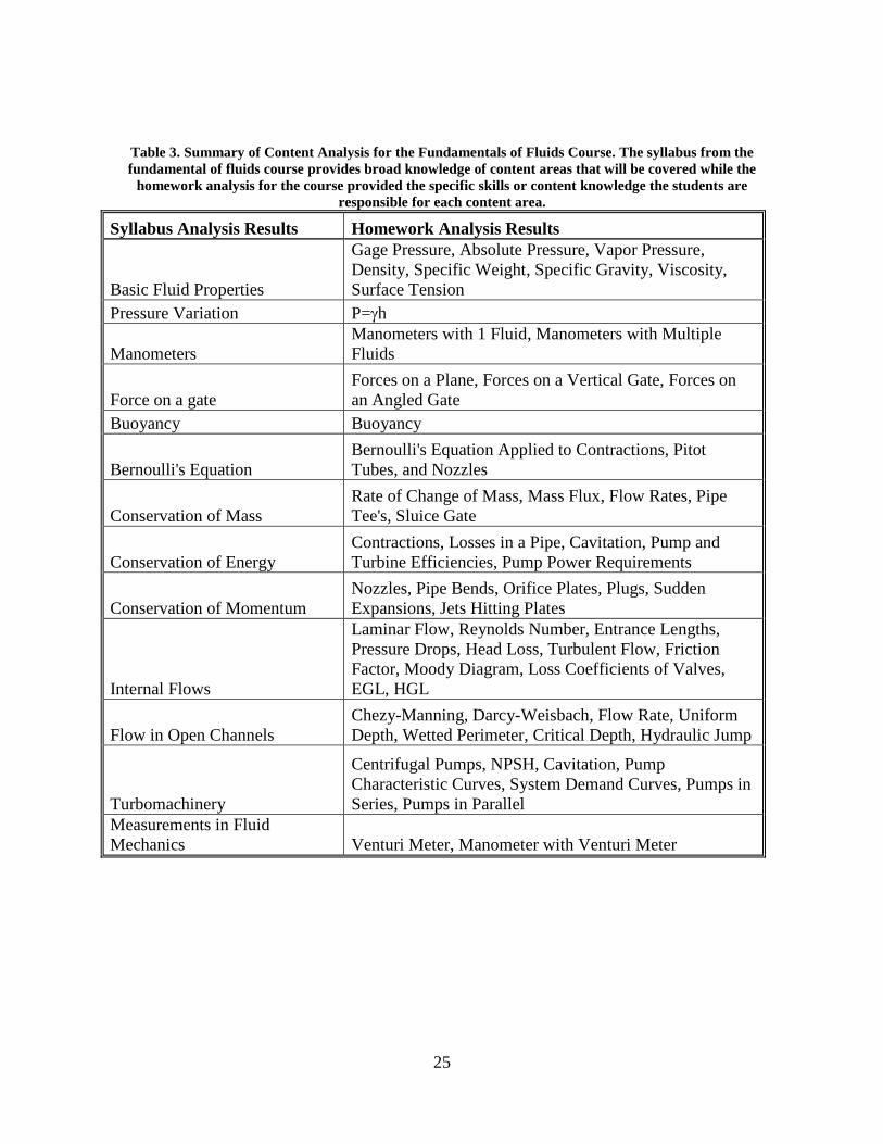
syllabus. Table 3 summarizes the key concepts of the course that resulted from analysis of the

syllabus and homework assignments.

The final step in determining the LE is accomplished through discussions with the faculty

member responsible for the Fundamentals of Fluids Course. As was mentioned earlier, the

faculty member will have the best understanding of student difficulty areas, important concepts

for later courses, and important concepts for the students' career. The topics that were chosen for

a LE usually met several of the following criteria:

• Students traditionally found this content difficult • Students would most likely need this content in their future coursework • Students would need this content in their future careers • Students would benefit from establishing real-world relevance • Students would benefit from a hands-on experience with a theoretical concept • Students would benefit from proper timing of course lectures and LE Table 4 is a list of the content covered in the old and new laboratory experiences for the

Fundamentals of Fluids course. It should be noted that in the same lab time period the number of

topics covered with LE increased from 16 to 40. With the establishment of the learning

objectives for the LE complete, the next step is to develop the laboratory equipment.

25

Table 3. Summary of Content Analysis for the Fundamentals of Fluids Course. The syllabus from the fundamental of fluids course provides broad knowledge of content areas that will be covered while the

homework analysis for the course provided the specific skills or content knowledge the students are responsible for each content area.

Syllabus Analysis Results Homework Analysis Results

Basic Fluid Properties

Gage Pressure, Absolute Pressure, Vapor Pressure, Density, Specific Weight, Specific Gravity, Viscosity, Surface Tension

Pressure Variation P=γh

Manometers Manometers with 1 Fluid, Manometers with Multiple Fluids

Force on a gate Forces on a Plane, Forces on a Vertical Gate, Forces on an Angled Gate

Buoyancy Buoyancy

Bernoulli's Equation Bernoulli's Equation Applied to Contractions, Pitot Tubes, and Nozzles

Conservation of Mass Rate of Change of Mass, Mass Flux, Flow Rates, Pipe Tee's, Sluice Gate

Conservation of Energy Contractions, Losses in a Pipe, Cavitation, Pump and Turbine Efficiencies, Pump Power Requirements

Conservation of Momentum Nozzles, Pipe Bends, Orifice Plates, Plugs, Sudden Expansions, Jets Hitting Plates

Internal Flows

Laminar Flow, Reynolds Number, Entrance Lengths, Pressure Drops, Head Loss, Turbulent Flow, Friction Factor, Moody Diagram, Loss Coefficients of Valves, EGL, HGL

Flow in Open Channels Chezy-Manning, Darcy-Weisbach, Flow Rate, Uniform Depth, Wetted Perimeter, Critical Depth, Hydraulic Jump

Turbomachinery

Centrifugal Pumps, NPSH, Cavitation, Pump Characteristic Curves, System Demand Curves, Pumps in Series, Pumps in Parallel

Measurements in Fluid Mechanics Venturi Meter, Manometer with Venturi Meter

26

Table 4. Content Areas Covered in Laboratory Experiences. The last two columns contain specific content areas that are covered in the LE. The content areas that are covered by the LE have significantly increased

through the redesign of the LE from16 to 40learnign objectives. General Content Area Content Areas Covered by

Previous Laboratory Experiences

Content Areas Covered by New Laboratory Experiences

Fluid Properties Basic units, mass and weight properties

Basic units, mass and weight properties, vapor pressure

Fluid Statics Pressure, pressure measurements, buoyancy

Pressure, pressure variation with elevation, pressure measurements, hydrostatic forces on plane surfaces, buoyancy, and stability

Flowing Fluids and Pressure Variation

Velocity, flow visualization with streaklines, laminar and turbulent flows, Bernoulli’s equation

Velocity, flow visualization with streaklines, laminar and turbulent flows, Bernoulli’s equation

Control Volume Rate of flow, control volume approach, continuity equation, momentum principle, derivation of the energy equation

Flow Measurements Measurement of velocity (propeller based instrument)

Measurements of velocity: propeller based instrument, Parshall Flume, weirs, orifice, venture meter

Differential form of Fundamental Equations

Continuity equation, momentum equation derivation, energy equations

Flow in Conduits Laminar flow in pipes, turbulent flow in pipes

Laminar flow in pipes, turbulent flow in pipes, flow losses from fittings, pipe systems, hydraulic and energy grade lines

Turbomachinery Radial-flow pumps, suction limitations, cavitation, pumps in series, pumps in parallel

Open Channel Flow Uniform flow, similitude- Froude Number, specific energy, hydraulic jumps

Uniform flow, similitude- Froude Number, specific energy, hydraulic jumps

Total Areas Covered 16 40

27

3.1.3 Development of Laboratory Equipment

Once the desired learning outcomes were developed, it was now time to develop the necessary

laboratory equipment. In a traditional product design cycle the development of laboratory

equipment would involve idea generation, idea selection, and detailed design. In our process, this

step and the following step, development of curriculum, are the instructional design equivalents.

During the development process decisions were made to either utilize existing equipment or

develop new equipment.

3.1.3.1 Utilizing Existing Equipment

There are many benefits to utilizing existing equipment. The most obvious is the financial

savings of using a current apparatus. There is also the time savings of not designing and

fabrication a completely new device. Most of the existing equipment is 20-30 years old and not

portable in nature. Therefore, most of the equipment was not able to be reused in the new LE.

A flow visualization table was reused instead of designing and fabricating a new device.

This device produced a well-developed flow stream that objects could be placed into and the

streaklines of the fluid as it moved around the object could be visualized. The old device used

red dye that would be put into the water in three locations using a reservoir cup and three

needles. Unfortunately, since the system circulates the water, the water became red rather

quickly and required draining during the laboratory in order to allow visualization for all of the

objects placed in the flow stream.

There is a commercially available fluid additive to help visualize fluid flow patterns. The

additive can be bought from the online store Steve Spangler Science and is called Pearl Swirl ®

(http://www.stevespanglerscience.com/product/1218). Each laboratory session requires only 1.5

28

bottles for a cost of just $10. The additive makes the water “shimmery” and it is possible to

visualize the flow patterns around an object. This modification has several benefits over the old

approach. The water does not need to be changed during the LE; it usually only needs to be

changed from one lab day to the next. It also provides a better visualization of the flow patterns

before, and especially after the object. It is now possible for students to visualize eddies after an

object and even see where the fluid changes directions and flows “upstream”. The final benefit of

this material is that it will fall out of solution when the velocity of the solution decreases

substantially. Therefore students can see where the stagnation point occurs as well as the

boundary layer.

3.1.3.2 Developing New Equipment

The developing of new equipment is a resource intensive process. It requires time, money,

proper facilities and equipment, and experienced personnel. Therefore it is critical to create as

few pieces of equipment as possible to minimize the resource requirements. This can be

accomplished by designed and creating multi-functional devices. The approach to accomplishing

this as well as some examples will be discussed in this section. The justification for the material

choices and measurement systems will also be discussed.

In order to develop as many multi-functional devices as possible a clear understanding of

all of the content that will be covered in the LE is required. This information is now readily

available after completing step 2 in our design process, Determination of Laboratory Curriculum.

After grouping the content areas into related categories it was determined that 13 separate LE

would be required to meet the educational needs of the students. A list of the LE and the required

device is shown in Table 5. Through careful planning, only 6 new devices were required. Multi-

purpose device 1 is shown in Figure 5 to clarify the definition of a multi-purpose device, the key

29

to a small number of required devices. The small number of devices created a substantial savings

in time and money. Images and a brief description of each device are shown in Figures 5 through

13, further information and setup is described in Appendix A.

Table 5. Laboratory Experiences and Device Types. The LE’s listed on the left side require some device in order to be conducted. There are three different types of laboratory devices: multi-purpose devices are used in multiple LE, Unique devices are used for only 1 LE, and Existing devices have been modified from their

original design or usage to improve learning.

30

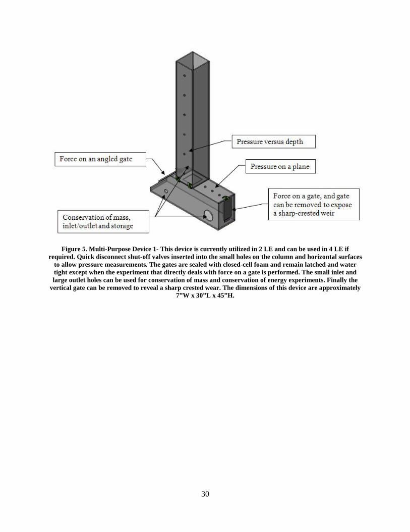
Figure 5. Multi-Purpose Device 1- This device is currently utilized in 2 LE and can be used in 4 LE if required. Quick disconnect shut-off valves inserted into the small holes on the column and horizontal surfaces

to allow pressure measurements. The gates are sealed with closed-cell foam and remain latched and water tight except when the experiment that directly deals with force on a gate is performed. The small inlet and large outlet holes can be used for conservation of mass and conservation of energy experiments. Finally the

vertical gate can be removed to reveal a sharp crested wear. The dimensions of this device are approximately 7”W x 30”L x 45”H.

31

Figure 6. Multi-Purpose Device 2- The rectangular box with the tube extending from it is used in a buoyancy LE and a specific weight LE. The spout allows water to flow from the container as the different objects that are on the table are placed into the container. The water is then collected and measured with the graduated cylinder and verified with the computer scale on the right of the picture.

The material selection choice was based on ease of fabrication and material properties

that would aid in student learning. It is not beneficial to save $10 in material cost if it requires an

additional 2 hours of machining time. Machining time if billed is currently around $45-80/hour.

Clear acrylic was used for the construction of our containers, flumes, and most devices. Since the

acrylic was clear, it allows students to visualize the water in the devices. Acrylic is also easy to

machine and can easily be joined together with a solvent, methylene chloride. Machinists in the

Swanson School of Engineering have substantial experience in creating acrylic water tight boxes

and provided a great resource during the design of these devices. In our devices that utilized

piping systems the material of choice was copper or PVC. PVC was chosen most frequently

because of its ease of assembly with just glue. There will not be high pressure water through

32

these pipes so schedule 40 was also specified. Schedule 40 PVC pipe can safely handle pressures

below 290 PSI; our experiments will never exceed 60 PSI. Copper pipes were only used when

absolutely necessary due to the increased cost of material and the skill and time required to sweat

joints.

The data acquisition component of any LE can be very substantial. The ITL that were

mentioned earlier requires the use of over $14,000 of data acquisition software and hardware for

each student station. This far exceeds our constraint of $6,000 for the entire project. After

substantial searching of different data acquisition systems the PASCO Pasport® system was

selected. It had the cheapest price and was able to meet all of our measurement needs. The

system is very user friendly and a program tailored for each lab can be quickly created and stored

on the computer for future lab teaching assistants to utilize. The sensors are easy to switch and

up to 3 channels of data can be recorded at anytime. The only significant limitation of the system

is the lack of accuracy of certain sensors. For example, it is sufficient for creating laboratory

pressure readings that are within 1-5% of theoretical values but the system is not capable of

recording more accurate readings. A typical pressure sensor system that would maintain an

accuracy of 1.5% is over $400 with only marginally better performance. The designers decided

to overlook the accuracy deficiency because the learning objectives would most likely still be

met and a greater chance of meeting the cost constraint could be realized. A consistent system

also reduces the time impact of the teaching assistant to learn the new sensor/software.

3.1.4 Development of Supporting Material

Curriculum according to Webster’s Dictionary [Curriculum, 1954], is the set of courses

constituting an area of specialization. In formal education, curriculum is also defined as the set of

33

courses and content offered at a school or university. The latter definition in our following

discussion; curriculum is the content of the LE for the Fundamentals of Fluids course. This

includes the teaching assistant training manual, student laboratory handouts, the data acquisition

program when applicable, and the overall flow of the LE. The approach to develop the

curriculum will be discussed in this section. Particular attention will be given to the method and

beliefs that were applied to this step in the design process.

Curriculum involves more than just the materials that are developed; it involves the

timing of the learning opportunities. The original LE were not could have been better

synchronized with the lecture and homework. It is logical to believe that learning opportunities

in the laboratory and in the class that are coincidental will improve student learning. The need

for students to visualize classroom theory with real-world examples has been mentioned several

times already. The alignment of the laboratory and lecture experiences was a priority in the

redesign of the LE curriculum. The results of this effort can be seen in the most current syllabus

found in Appendix C. Both the LE and lecture are aligned to cover the same content and each

will either reinforce or introduce common content.

The development of curriculum phase is depicted as following the development of lab

equipment phase in Figure 4, the design process overview. However, this stage does not start

when the equipment phase finishes. The devices are designed with a vision of what the LE

experience will involve. It is more accurate to think of the two stages beginning together with the

effort being spent on curriculum and equipment. Once the overall design of the LE is determined

and how a piece of equipment will be utilized efforts were focused on the design and fabrication

of the equipment. With the equipment completed the focus is then on the curriculum to

accompany the device. By using the above approach it is very likely that the equipment will meet

34

our curriculum requirements and excessive time developing curriculum before the device is not

required.

The instructional design concept of curriculum development that was adopted is rapid-

prototyping. Since curriculum has a relatively low impact on resources it is beneficial to apply

this type of design. In developing the curriculum, the main resource that was used is time. From

our earlier design steps, an initial idea of what the students should learn and accomplish in each

LE was created. The curriculum was then developed based off of research and experiences as

instructors to provide the students with the learning opportunities to acquire the knowledge and

experience that were important for the activity. In developing curriculum, a lot of time and

energy can be used in predicting how students will understand a step, what misconceptions they

may carry, and what they will walk away from the LE understanding. Using previous knowledge

and experience a “best-guess” of what will work for the students was developed. Educational

systems have so many factors and influences that it is impossible to guarantee that one approach

will work in all situations. Excessive time and effort can be spent predicting the effectiveness of

curriculum, it is therefore beneficial to develop a reasonable set of curriculum and conduct a

pilot study. The methods and benefits of a pilot study are discussed in the next section. Since a

rapid prototyping approach was followed, the curriculum development step is the most revisited

in our design process. Over time, the curriculum has changed from a “pretty good” level to a

very effective level. This iteration process is also described later and since it is a critical part of

curriculum development it is briefly mentioned here.

Through the rapid prototyping approach there were several over-arching principles that

were present in the LE. The LE is an opportunity for students to have more practice on key

concepts in the course and LE are a logical place for extending homework and class concepts. It

35

has previously been shown that students learn better when they realize the real-world

applications of the content that they learn. Curriculum was developed that allowed students to be

“dam engineers”, “load masters” for coal barges, and even “plumbers” soldering pipes. Another

key principle that the LE curriculum develops is the ability to design a lab experience. In the

past, students would just follow a set of steps and record their data to prove a concept. In the new

LE, students are often asked to design the experiment based off of the available equipment,

determine how to reduce error, and determine what variables are necessary to control and

measure. Finally, the curriculum must still allow students to visualize some of the theoretical

concepts discussed in class to aid in the students’ understanding. These elements are present to

some degree in each of the 13 LE developed for the course, the LE have a variety of approaches

to keep the labs interesting and to meet more student needs.

The final modification of the LE curriculum was the introduction of guided problem-

solving sessions. In the week preceding an exam, students review a previous year’s exam in their

scheduled laboratory period. This allows the teaching assistant to properly model problem

solving strategies, the teaching assistant solves the problems by thinking aloud as they work on

the board. The students are expected to at least attempt to develop a plan on how to solve the

problem before the laboratory period. This session is optional and many students utilize it to

benefit their learning experiences.

3.1.5 Pilot Study and Assessment

The pilot study and assessment phase are a key factor in ensuring the best LE possible. This step

correlates with the traditional prototyping testing and design verification phases that are common

in PD. Pilot studies and assessment are always critical in ID; however, they are even more

36

critical in the design process because the curriculum was developed utilizing a rapid-prototyping

model. The model requires assessment and formative feedback to create higher quality

curriculum each cycle since many assumptions and “best guesses” occur in the curriculum

development phase. Summative feedback is not necessary for the design process but it useful for

dissemination and will be discussed in a later chapter. In this section, the pilot study schedule

and an assessment tool that was developed for the LE will be discussed.

3.1.5.1 Pilot Study

The pilot study was done in several stages over the course of two years. The main objective of

the pilot study is to gather information about the quality of the curriculum and equipment that

was created. The initial pilot study was very minor. One modified LE was conducted in the fall

of 2007. In hind-sight, it would have been advisable for quality of summative assessment data to

not change the control group’s LE. Each subsequent term new LE were piloted, Table 6

summarizes our pilot study implementation schedule. By spreading the implementation over

several semesters the designers were able to learn from the results of piloting each new LE. The

formative assessments of the piloted LE allowed the design of later curriculum and equipment to

benefit from our growing knowledge and experience related to students’ learning in the

laboratory environment of a fluids course. Due to limited resources, specifically development

time in the summer and fall of 2008, two of the new LE have not been piloted as of yet. It is the

hope of the author that they will be ready for pilot testing this semester. These 2 LE are

completely new to the course and would only further enrich student learning.

37

Table 6. Pilot Study Schedule. The new LE were phased into the fundamental of fluids course, the term denotes the semester that the new LE was first used. The LE after the pilot study are improved and then

become a permanent part of the curriculum.

3.1.5.2 Assessment

An ideal situation for any instructional designer is to use readily available assessment tools.

Earlier in Section 2.4 the Fluid Mechanics Concept Inventory was discussed and it was shown

that the authors were unhappy with its current performance. Another option would be to use

standard test questions from year to year. However, in many institutions student populations are

very talented at finding old exams to view and practice with. A test with the same question from

one semester to the next may be a measure of a student’s ability to find old tests more than a

measure of the affect of the new LE. Final exams are usually immune to the problem mentioned

above but it would be difficult to have a final exam that could assess all of the LE plus other

critical material that is covered in the course. The designers therefore chose to create a self-

38

assessment survey to assess the effectiveness of the new LE. An additional satisfaction type

survey was also created as a back-up assessment tool.

The development of an assessment tool requires some resources to complete but insures

that the tool will meet our specific requirements. The development of the self-assessment survey

was relatively quick when compared to developing a set of conceptual questions. The survey is

intended to elicit a student’s self-assessment of their knowledge of a particular content topic. The

process begins by determining all of the possible topics that could be covered in the

Fundamentals of Fluids course. Determining the topics can be accomplished by looking at the

table of contents of the course’s textbook and adding any topics that are covered without the use

of the textbook. The relatively large number of topics serves two purposes. First, the topics that

are not covered in the course help to verify the tools effectiveness. Students should not show a

significant gain for topics that are not covered in the course. Student learning may occur in other

courses or through experiences in life but the majority of these topics should not show a

significant gain if the tool is effective. The second benefit is to provide a baseline of data that can

be recorded. If an instructor decides to cover a new topic, or add another LE there is a sufficient

control group that the group which experienced the new curriculum can be compared too. Once

all of the possible topics are determined, the survey is created. It is standard to use a 5 point

Likert scale with 1 representing “never heard of it” and 5 represents “extensive knowledge”. The

survey has 96 assessment points, see Appendix D, and has been administered as a pre- and post-

instruction survey to 2 groups. The third group is currently being evaluated this semester. The

actual assessment results are discussed in Section 5.2.1.

The development of our evaluation form served several purposes. First of all, it would

provide a more common assessment of changes to the course. Student perceptions about the

39

quality of the lab or their experiences are often shown to justify the impact of a new pedagogical

approach. Our evaluation form was divided into three sections to answer different questions:

• What components of the entire course helped the student learn the most • Did engineering or lifelong learning abilities improved as a result of this course • What are the opinions of the LE? Our evaluation survey was also a back-up to the self-assessment survey. Although the self-

assessment survey has been shown to be successful in literature and through personal experience

of the course coordinator, this was a first attempt at applying the survey to fluid mechanics and

difficulties could arise. This survey has a total of 33 topics and can be found in Appendix E. The

results of the analysis of this survey’s data are also contained in Section 5.2.2.

Relevant assessment and feedback information can be gathered through non-quantitative

means as well. Each LE was assessed for its ability to perform as designed, through observations

of the students in the laboratory and also through the laboratory reports that were submitted a

qualitative impression was made about each LE. During the LE, the directions or information

provided to the student were misleading or not always sufficient. Since the designer was also the

teaching assistant, it was easy to record these problems and make modifications to the

curriculum to improve the LE after each pilot study. This process is usually not very time

consuming but seems to be improving the quality of the rapid-prototype. The students’

laboratory reports are also analyzed to determine if students are realizing the main learning

objectives of each LE. Again, if the designer/teaching assistant sees a disparity between what the

students were intended to learn and what they actually learned, the curriculum can be modified

for the next pilot study. It was very beneficial for the curriculum developer to also be the

teaching assistant, immediate and very accessible feedback was easily transferred to improved

prototype quality.

40

3.1.6 Finalization of Lab Equipment and Curriculum

The finalization of the lab equipment and curriculum is nearly complete. Based off the results

from the pilot study and assessment data several design changes were made. For the most part,

the laboratory equipment was well developed and has only received minor modifications with

the exception of one LE. The conservation of momentum LE is still not producing meaningful

and useful data for students. Several modifications to the equipment have been completed, and

each time we have not realized any significant increase in performance. Final suggestions for this

LE will be made later in the future work chapter. The overall success of the equipment in the

pilot study is satisfying to the designer. Unlike the written curriculum, the equipment was not

designed in a rapid-prototype fashion. Considerable planning, design experience, computer aided

design, discussions with the faculty responsible for the course, and the Swanson School of

Engineering’s Prototype Machine Shop manager provided many benefits. Without these

resources many of the devices would most definitely need to be redesigned.

The finalization of the curriculum is an ongoing process this semester. The final pilot

study should be sufficient to finalize the curriculum for the labs that have been created. These

components of the overall design have seen many modifications. The modifications were to be

expected due to the rapid-prototyping approach to the curriculum development. The final

handouts can be found in Appendix B. A more detailed description of the equipment setup and

overall progression of each LE are found in Appendix A. The goal of this phase in the design

process is to develop sufficient material to insure that this LE can be duplicated in this

department in subsequent semesters with different teaching assistants assigned to the course.

There are not sufficient time resources in the scope of this project to develop the necessary

equipment drawings and specifications for duplications at other universities.

41

3.2 ITERATIONS IN THE DESIGN PROCESS

It has already mentioned that the design process is not linear; it has several iteration loops that

are important to discuss. The main results of these iterations also fall into two categories,

improvements or expansion. In this section, the iteration process for the project is discussed as

well as the results of the iteration activity.

Most of the design iterations occur as a result of the pilot study, only rarely was there

iteration in the development of equipment phase. When iterations did occur in the equipment

phase, it usually resulted from feedback from the fabrication activity. The designs were well

thought out, but occasionally design choices resulted in difficulties in fabrication. When this

occurred, the initial design was reevaluated and modified if it would improve fabrication and

maintain the same level of functionality. As a designer, it is important to be flexible and

constantly monitoring any feedback available to improve the overall design.

The first iteration loops occurs after the pilot study and assessment phase and returns to

the development of lab equipment phase. Feedback from lab reports, being a teaching assistant in

the LE, and discussion with students provides important information. As mentioned in Section

3.1.4, the development of laboratory equipment and curriculum occur in almost a parallel

fashion. The feedback information is equally important to each. The curriculum tended to be

revised more frequently, mostly to improve directions or the content of the laboratory handouts.

If students did not have the intended learning experience the curriculum was modified to

improve its quality. Most of the equipment remained the same after the pilot study with the

42

exception of the flume and momentum experiments. Both of these were modified to improve the

quality of data that could be gathered. The flume required a redesign of the baffles to help

develop the flow and the addition of a few more components to increase flow in the piping

system. The initial piping for the pump component of the flume was not well planned, and the

changing of the location of the pump and the addition of an elbow were required to improve the

flow characteristics of the system. The momentum experiment is still not working as effectively

as possible. Another redesign that may involve a different example of the conservation of

momentum may be required, or the experiment may improve with more pressure. Currently, the

experiment’s flow and pressure are created by two pumps in series; the resulting pressure is only

about 5 feet of water (2.17 PSI). If the experiment is connected to the pressure available from the

water supply in Benedum the pressure would be close to 100 feet of water (43PSI). the increased

pressure would result in an increase in the force to hold the 180 degree bend in place and may

allow students to actually gather several data points for their experiment. These are just a few

examples of how this iteration loop improves the design.

A larger iteration loop surfaced as the project progressed. An iteration loop that flowed

back to the determination of laboratory experiences phase emerged. When most of the LE were

completed and conducted, ideas for extensions or new learning objectives always seemed to

surface. Perhaps the visualization of the theoretical concepts not only benefits the students but

also may help designers. This phenomenon is also not uncommon in the PD world; in PD it is

known as project drift. The initial outcomes and goals of the product are realized and the person

in charge begins to think how nice it would be if the product could do, X, Y, and Z as well.

Many times project drift was allowed to occur and the LE were expanded to include the new

possibilities in subsequent prototypes. This was allowed to occur if the overall project would still

43

be able to stay within the constraints that were established in the first phase. Each expansion

requires resources and it is important to decide which expansions are most needed or will have

the greatest impact and then pursue those concepts.

44

4.0 NEWLY DESIGNED LABORATORY EXPERIENCES

The product of the design process is both the equipment and the associated curriculum for each

LE. The equipment is relatively easy to set-up and use but a manual for the teaching assistant

will be beneficial. This manual is intended to insure that the next teaching assistant can

effectively teach the LE. In order to meet this need, the designers believe it is important that the

manual contain the following information:

• learning objectives • over-arching principles • common areas of student difficulty • warnings to increase accuracy or protect the equipment • data acquisition setup (if applicable) • output screens of data acquisition software • pictures of equipment • setup of equipment

The manual is therefore a description of each LE and can be found in Appendix A. The

associated laboratory hand-out can be found in Appendix B. Table 7 is an aid to understand

which device and hand-out is related to which LE. The teaching assistant laboratory manual was

created to improve student learning. A teaching assistant who better understands the philosophy

and objectives of a lab will perform better and improve student learning more than one who only

knows how to follow the procedures.

45

Table 7. Summary of Products for all of the New Laboratory Experiences. Each LE has an associated lab number for the ancillary material that was created for it and a specific device that must be used with the LE.

46

5.0 DATA ANALYSIS

The field of engineering education is continuing to grow and must maintain quality data analysis

to improve the acceptance of its efforts and results by the entire engineering community. To this

end, a self-assessment pre- and post-survey was developed to provide a more elegant approach to

assessment. A more standard evaluation survey was also administered to the students when they

finished the course each semester. During our preliminary analysis, the change in mean scores

between the new LE to existing LE provided very promising results. Our primary data analysis is

discussed in the following sections of this chapter.

The preliminary analysis of our data was based on the difference in the average percent

of gain realized for each question on the self-assessment survey for fall 2007 students and spring

2008 students. The analysis was completed through the following steps:

• Determine each students change from pre- to post-instruction survey for each question • Divide the results of step 1 by the possible gain [5(the maximum value on Likert Scale) minus the pre-

instruction ranking] and multiply by 100, this gives the percent of gain realized • For each question, determine an average student response by finding the average percent of gain realized • Find the difference between the two data sets (fall 2007-control, spring 2008-treatement) for each question. An initial analysis showed that students had a greater increase in their perception of

understanding for topics that were covered in new labs. The data is summarized in Table 8, of

the 8 largest gains 6 of them occurred for concepts covered in the new LE. This analysis lacks

any statistical approach and a more robust analysis should be performed to verify that these

changes are indeed significant.

47

Table 8. Summary Table of Concepts with the Largest Difference in Percent of Gain Realized. Shaded regions are concepts covered with new laboratory experiences. The students in each group were given a self-

assessment survey pre- and post- instruction. The last column represents the change from one semester to the next. (Fall 2007 n= 37, Spring 2008 n= 13) *- See Appendix D for a description of the concept number

5.1 STATISTICAL ANALYSIS APPROACHES

The results from educational research are often reported by measuring the effect size. This

method is relatively easy and can be accomplished using most spreadsheet programs. However,

as was mentioned earlier, it is not advisable to use data analysis approaches for continuous data

on ordinal data. Since the Likert Scale surveys are ordinal a Mann-Whitney U test was conducted

in the analysis. This test cannot be completed using a spreadsheet but it can be easily conducted

using statistical analysis software. These two steps will be described in this section.

48

5.1.1 Effect Size

The effect size is a relatively easy calculation. The purpose of the statistical analysis for the

available data is to determine if the new LE had an impact on learning fluids, and if there was an

impact, was it a positive or negative impact. This hypothesis would be proven if the two groups

of students had different average rankings on the self-assessment survey. At the beginning of this

chapter it was demonstrated that the LE did have an increase in understanding, but was this

change significant? The effect size calculation is a common measurement found in the

engineering education literature. The higher the value the more effect has occurred. A value

above 0.5 is considered to be worthy of reporting, a value of 0.8 is considered excellent, and 1.0

is rare. The effect size was determined between students in the fall of 2007 (control group) and

the students in the spring of 2008 (experimental group) for each of the 96 self-assessment survey

questions. The method to calculate effect size is shown below:

• Determine the difference from pre-to post- instruction for each student for each question • Determine the mean of the above step of each question for each group of students • Determine the standard deviation of the first step for each question for each group of students • Divide the difference in the mean by the pooled standard deviation • The standard deviation can be found by using the equation in Figure 6.

• Figure 7. Pooled Standard Deviation – This equation is used to determine a combined standard deviation for

multiple datasets. (n=number of samples in the data set, s=standard deviation of the dataset, k=number of datasets)

The effect size was calculated in a similar manner for the evaluation surveys except there was

only a post-instruction evaluation survey given to the students. The analysis is based on the mean

scores for the surveys of the two groups; both sets of results are reported later in this chapter.

49

5.1.2 Mann-Whitney U Test

The Likert self-assessment survey and evaluation survey are ordinal and are more appropriately

evaluated using a non-parametric test. The Mann-Whitney U test (MWU) is the best test for our

data. The data collected is normally distributed, but has a relatively small sample size, the

maximum set of students’ surveys is 37 and the minimum is 13. The MWU will be used to

determine if there is a significant difference in the scores from the control group to the

experimental group. A significant result occurs when the hypothesis that the two datasets are

equal is false.

The MWU is simple in nature but would require substantial time if conducted by hand,

therefore, Mintab ® was used to perform this analysis. Minitab was used to determine a

significance level when the distributions of one set of data are not equal to the distributions of

another set of data. The lower the significance level, the more likely the two sets of data have a

different mean value. Remembering from basic statistics that the significance level is 1 minus the

confidence level, the significance level was set to be 0.05, a common value in educational

research literature. Therefore there would be a 95% confidence level that the two values are

statistically different if the significance is less than 0.05. As the significance increases it is not

possible to say that the two groups of data are significantly different. The exact approach used in

a MWU can be found in a statistical textbook [Kreyszig, 1970]. The approach to performing the

MWU using Minitab can be found in a user book by Ryan et al [Ryan, 2005]. The results of

Minitab give a significance level that the two sets of data would be considered different.

Therefore, a very small number demonstrates a very strong statistical difference in the two data

sets.

50

5.2 RESULTS AND DISCUSSION

Significant results will only be reported in this section. During the statistical analysis, it became

apparent that it will not be possible to determine the effectiveness of each lab with our

assessment methods. Therefore, results from tests and finals conducted during different

semesters are also included. The use of ABET criteria has also been used to determine the impact

of the LE. These results allow the observation of the general effect on overall student

performance in the course.

5.2.1 Self-Assessment Survey

Although the literature showed promise in the self-assessment survey approach, the results do

not permit considerable conclusions from the data. The intention was for the survey to show a

difference in students’ perception of understanding in specific content questions. The tool was

designed to measure the impact of the new LE on student learning when compared to old LE.

There were 96 concepts on the self-assessment survey, of those 96 only 5 demonstrated a

significant effect; as shown in Table 9. The first two concepts related to manometers which has

the same curriculum between the two semesters. However, the students showed a significant

change form one semester to the next. In education there are a substantial number of variables. It

is difficult to say why students showed a substantially gain in this area, an unfortunate possibility

is that the survey is not working well. The next two topics received were taught with new LE in

the experimental group. It is satisfying to see a reportable effect size; however, more data will be

needed to support that the LE influenced this gain. This material was covered on the first exam

and the results of the first exam scores will be discussed later in this chapter. The last topic,

51

viscosity, was only discussed in lecture and there is no evidence that the lecture was changed

substantially from one semester to the next. Together these results discount the legitimacy of the

self-assessment survey that was developed as a tool in determining the effectiveness of changing

LE.

Table 9. Significant Effect Size Results for the Self-Assessment Survey (n=50). Effect sizes greater than 0.5 are considered to be significant, the larger the number the more different the mean results are from each group, Fall 2007 and Spring 2008 students. Concepts 3 and 12 were not treated differently; the remaining

concepts had new LE for the Spring 2008 semester.

The confidence in the self-assessment survey to differentiate the student performance due

to different learning opportunities was further decreased after a MWU was conducted. Since the

data is ordinal, this is the more accurate test of significance. The results of this test are shown in

Table 10. Of the 15 concepts that showed a significant difference in the scores, only 2 of them

received any substantially different treatment from the control group to the experimental group.

Again, it is difficult to understand let alone control all variables in an educational experiment but

the appearance of only 2 concepts that were treated with the new LE raises more concern for the

test validity. The other 13 concepts received the same treatment and it is assumed that they

52

should not be significantly different; this however is not the case. There is a large chance that the

self-assessment survey did not work effectively in measuring the impact of the new LE.

Table 10. Mann- Whitney U Test Results for the Self-Assessment Survey (n=50). The self-assessment survey was given to students pre-and post instruction in two different semesters (fall 2007 and spring 2008). A

significance level below 0.05 are considered significant, the lower the number the more significant. Most of the concepts in this list are not covered or covered in the same manner from one semester to the next.

Therefore the quality of the test instrument is concerning since it cannot differentiate between material that is not covered, covered, or covered with new LE. *- represents a new LE for the spring 2008 students

5.2.2 Evaluation Survey

The evaluation survey contained 33 items, many of which were not relevant to the LE. This

survey did show some promising results for the new LE. This survey is vaguer than the self-

assessment survey but some general conclusions based off of some significant results in our

53

analysis can be made. Table 11 shows the result from determining the effect size for the 2 data

sets; survey items that showed an effect size above 0.5 from the fall 2007 semester to the spring

2008 are shown. The in-class review, which showed an effect size of 0.57, was not an addition to

the course and the gain was unexpected. The gain may be due to the change from one semester to

the next in the teaching assistant who provided the in-class review. Items 4, 7, 6, and 15 were

related to how much each item helped the students learn, a positive shift is beneficial for these

items. According to this data our labs improved the students learning. The improvement is either

due to the new LE or to the new teaching assistant or to a combination of these factors. Item 27

and 28 deal directly with the students’ opinions of the LE. 28 is obviously a beneficial change if

the results are negative, positive results occur when students disagree with this statement more if

the new LE are effective. From these two items it can be said that our labs are generally less

boring and engaged students more in the LE.

Table 11. Effect Size for Evaluation Survey (n=50). Students in the fall 2007 and spring 2008 completed a post instruction survey that was based on the LE and what helped them learn through the semester. The effect size

is a measure of the difference in the mean score between these two populations on the survey. Effect sizes greater than 0.5 are significant and the larger the number the greater the effect.

The analysis of the evaluation survey using the MWU provided similar results see the

summary in Table 12. The items that showed significant differences in the experimental and

54

control population were all related to the LE or the teaching assistant except for the last item,

lecture. The difference in lecture scores is an interesting result and may be due to the

substantially smaller class sizes that traditionally occur for this course in the spring semester.

The professor may be able to customize the learning experience better for the students with a

smaller class size. The rest of the results in Table 12 demonstrate that the new LE are having a

significant impact on the students’ learning, the lower the number the more significant. The

MWU does not differentiate positive or negative directions in the distribution of responses; it

only shows if there is a significant difference. Therefore it is important to clarify that the students

were less bored in the LE in the spring 2008 semester, this is easily seen in Table 11. Since it is

apparent that the new LE are having a positive effect, tests and final data will be utilized to try

and determine which LE or groups of LE are having the most effect.

Table 12. Mann-Whitney U test for the Evaluation Survey (n=50). Students in the fall 2007 and spring 2008 completed a post instruction survey that was based on the LE and what helped them learn through the

semester. A significance level below 0.05 shows a significant difference between the two populations.

55

5.2.3 Exam Data

There are 3 exams throughout the semester and one final in the Fundamental of Fluids course.

The first exam covers several concept areas: basic properties of fluids, pressure with depth,

pressure on gates, and conservation of mass. The second exam covers Bernoulli’s Principle,

conservation of momentum, and conservation of energy. The third test is a group test that

students traditionally do well on. The last exam that would be useful to analyze is the final.

Therefore the first and second exam may help us determine if each set of new LE made an

impact, and the final can measure overall improvements that are due to the new LE.

The first test covers material that was piloted first in the spring 2008 semester. This

would be the fundamental properties of fluids, force on a gate, and forces with depth. The

conservation of mass LE was introduced in the fall of 2007. Figure 8 shows the results for the

first test over the last 9 semesters. The table clearly shows an increase in student performance

once the new LE are piloted. This gain in performance remains in subsequent semesters. The

slight decrease that occurs after the spring 2008 semester may be due to the impact of the

temporary loss of lab space. The lab was basically conducted in a hallway that lacked basic

infrastructure for the lab. This area was also in the center of the construction offices and was

frequently disrupted by the construction of Benedum Hall. In the spring 2009 term, the LE has

moved to a room that is under construction in the basement. It is an improvement over the fall

2008 circumstances but it is not even close to an ideal learning environment. As a result, when

this data is combined with information from previous analysis it can be concluded that the new

LE that cover topics on the first test had a significant and real impact on the students’ learning.

The second test results, see Figure 9, show the highest average test 2 scores for the

semester that the material was first piloted. The new LE began in the spring of 2008 for the

56

material covered on the second exam. This includes the conservation of momentum and the

conservation of energy. The conservation of momentum laboratory has consistently performed

poorly and it is not surprising that the new LE has not shown a sustained impact. The other key

topic covered on this test is Bernoulli’s Principle. There is not a specific lab that can be used to

reinforce this concept at this time. In the future there will be a lab that deals with measurements

in fluids, and Bernoulli’s Principle will be applied in this lab. The impact of the negative learning

environment over the last two semesters may be hiding some of the gains that are occurring with

the new LE. From this data, it is difficult to determine if the new LE are positively or negatively

impacting the student performance due to the possible learning environment impact on learning.

Figure 8- Test 1 Results. The mean score for each semester is higher after the new LE have been implemented. These new LE provide more opportunities for learning and new areas of coverage in the

laboratory setting. Error bars are the standard error of the mean.

60%

65%

70%

75%

80%

85%

90%

95%

Sp05 Fa05 Sp06 Fa06 Sp07 Fa07 Sp08 Fa08 Sp09

Perc

ent C

orre

ct

Semester

Mean Percent Correct- Exam 1

n=25 n=58 n=17 n=61 n=27 n=47 n=16 n=61 n=35STDV= STDV= STDV= STDV= STDV= STDV= STDV= STDV= STDV=17.2% 11.9% 20.4% 12.6% 13.7% 14.7% 6.0% 8.3% 12.3%

57

Figure 9- Test 2 Results. The mean score for each semester has not consistently changed with the new LE being implemented. During the last two semesters the labs were conducted in adverse learning

environments and this may have negatively impacted the learning. The new LE do not show a statistically significant decrease in performance which is beneficial.

The final was the last set of data that was utilized in the analysis. The summary of

average scores on the final for the last 4 semesters is shown in Figure 10. The data for the spring

2009 semester is not available while this document is being written. The table shows a consistent

fluctuation between the spring and fall, according to the professor of this course, this trend

always seems to happen. Although this data does not show a significant gain, it does show that

the new portable LE do not cause a negative effect on student learning.

60%

65%

70%

75%

80%

85%

90%

95%

Sp05 Fa05 Sp06 Fa06 Sp07 Fa07 Sp08 Fa08 Sp09

Perc

ent C

orre

ct

Semester

Mean Percent Correct- Exam 2

n=25 n=57 n=17 n=61 n=27 n=47 n=16 n=61 n=35STDV= STDV= STDV= STDV= STDV= STDV= STDV= STDV= STDV=14.2% 10.8% 17.2% 13.7% 8.9% 10.0% 18.6% 12.4% 13.3%

58

Figure 10- Final Exam Results. The mean score for each semester does not show a statistically significant difference from year to year. A semester to semester variation does occur and this can be attributed to the different level of student performance. Usually students in the fall semester are on

track to graduate on time, while students in the spring semester are either transfer students or students who have fallen behind. The graph shows that there has not been a negative impact on

student learning with the new LE. Error bars are the standard error of the mean.

5.2.4 ABET Criterion

ABET certified engineering departments across the country are required to measure student

progress towards criterion. ABET Criterion 3, Program Outcomes, has several outcomes that the

new LE attempted to address throughout the course. For many semesters, the civil and

environmental engineering department at the University of Pittsburgh has been measuring the

results of an end of semester survey that determines if students feel the course they just finished

60%

65%

70%

75%

80%

85%

90%

95%

Sp05 Fa05 Sp06 Fa06 Sp07 Fa07 Sp08 Fa08

Perc

ent C

orre

ct

Semester

Mean Percent Correct- Final Exam

n=25 n=58 n=17 n=61 n=27 n=47 n=16 n=60STDV= STDV= STDV= STDV= STDV= STDV= STDV= STDV=11.9% 11.0% 15.6% 10.0% 10.7 % 12.9% 10.5% 10.0%

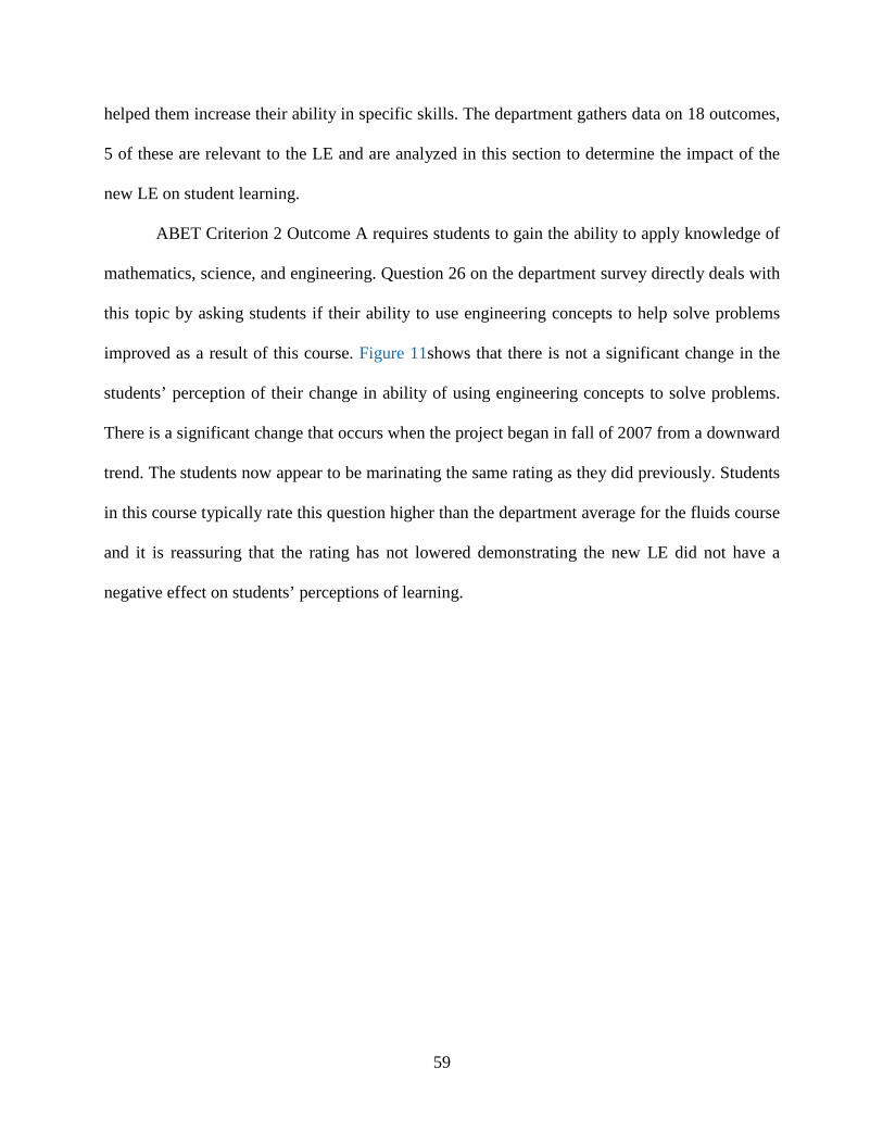
59

helped them increase their ability in specific skills. The department gathers data on 18 outcomes,

5 of these are relevant to the LE and are analyzed in this section to determine the impact of the

new LE on student learning.

ABET Criterion 2 Outcome A requires students to gain the ability to apply knowledge of

mathematics, science, and engineering. Question 26 on the department survey directly deals with

this topic by asking students if their ability to use engineering concepts to help solve problems

improved as a result of this course. Figure 11shows that there is not a significant change in the

students’ perception of their change in ability of using engineering concepts to solve problems.

There is a significant change that occurs when the project began in fall of 2007 from a downward

trend. The students now appear to be marinating the same rating as they did previously. Students

in this course typically rate this question higher than the department average for the fluids course

and it is reassuring that the rating has not lowered demonstrating the new LE did not have a

negative effect on students’ perceptions of learning.

60

Figure 11- ABET Criterion 2 Outcome A Results. Student responses to the statement: This course improved my ability to use engineering concepts to help solve engineering problems. Mean rating on a 5-point Likert

scale, 5 is the optimal response. The students’ perceptions regarding their ability to use engineering concepts to solve problems appear to be revitalized with the beginning of the project in the fall 2007 semester.

ABET Criterion 2 Outcome B requires students to gain the ability to design and conduct

experiments, as well as to analyze and interpret data. This key trait of an engineer is assessed

through question 27 and 28 on the department survey. Question 27 is related to the ability to

design and conduct an experiment; the results of this question are shown in Figure 12(A).

Question 28 relates to the students’ ability to analyze and interpret data, the results of this

question are shown in Figure 12(B). The results of both questions show that student learning

may slightly be improving with the new LE. As before, the downward trend that was occurring

before the fall 2007 semester was stopped and a new trend with a higher mean value appears to

be forming.

3.53.73.94.14.34.54.74.9

Sp05 Fa05 Sp06 Fa06 Sp07 Fa07 Sp08 Fa08

Mea

n Ra

ting

Semester

Results of the End of Semester Survey- Question 26

n=22 n=52 n=12 n=57 n=17 n=43 n=14 n=54 STDV= STDV= STDV= STDV= STDV= STDV= STDV= STDV=0.67 0.81 0.79 0.71 1.07 0.63 0.74 0.77

61

Figure 12- ABET Criterion 2 Outcome B Results. (A) Student responses to the statement: This course improved my ability to design an experiment to obtain measurements or gain additional knowledge about a process. (B) Student responses to the statement: This course improved my ability to analyze and interpret

engineering data.

2.8

3.3

3.8

Sp05 Fa05 Sp06 Fa06 Sp07 Fa07 Sp08 Fa08

Mea

n Ra

ting

Semester

Results of the End of Semester Survey- Question 27

n=22 n=52 n=12 n=57 n=17 n=43 n=14 n=54 STDV= STDV= STDV= STDV= STDV= STDV= STDV= STDV=1.39 1.16 1.42 1.05 1.29 1.14 1.16 0.88

A

3.0

3.5

4.0

4.5

Sp05 Fa05 Sp06 Fa06 Sp07 Fa07 Sp08 Fa08

Mea

n Ra

ting

Semester

Results of the End of Semester Survey- Question 28

n=22 n=52 n=12 n=57 n=17 n=43 n=14 n=54 STDV= STDV= STDV= STDV= STDV= STDV= STDV= STDV=0.74 0.83 1.21 0.68 1.11 0.82 0.55 0.71

B

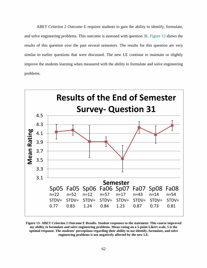
62

ABET Criterion 2 Outcome E requires students to gain the ability to identify, formulate,

and solve engineering problems. This outcome is assessed with question 31. Figure 13 shows the

results of this question over the past several semesters. The results for this question are very

similar to earlier questions that were discussed. The new LE continue to maintain or slightly

improve the students learning when measured with the ability to formulate and solve engineering

problems.

Figure 13- ABET Criterion 2 Outcome E Results. Student responses to the statement: This course improved my ability to formulate and solve engineering problems. Mean rating on a 5-point Likert scale, 5 is the optimal response. The students’ perceptions regarding their ability to use identify, formulate, and solve

engineering problems is not negatively affected by the new LE.

3.1

3.3

3.5

3.7

3.9

4.1

4.3

4.5

Sp05 Fa05 Sp06 Fa06 Sp07 Fa07 Sp08 Fa08

Mea

n Ra

ting

Semester

Results of the End of Semester Survey- Question 31

n=22 n=52 n=12 n=57 n=17 n=43 n=14 n=54 STDV= STDV= STDV= STDV= STDV= STDV= STDV= STDV=0.77 0.83 1.24 0.84 1.23 0.87 0.73 0.81

63

ABET Criterion 2 Outcome K requires students to gain the ability use the techniques,

skills, and modern engineering tools necessary for engineering practice. This outcome is

evaluated with question 32. Figure 14 shows that there has been no negative effect from the new

LE.

Figure 14- ABET Criterion 2 Outcome E Results. Student responses to the statement: This course improved my ability to use laboratory procedures and equipment. Mean rating on a 5-point Likert scale, 5 is the optimal response. The students’ perceptions regarding their ability to use laboratory procedures and

equipment are not negatively affected by the new LE.

Although the use of ABET criterion did not show that the new LE improved student

outcomes it reinforces the concept that student learning was not negatively affected. As the new

LE became more a part of the curriculum the trend in all of the questions were positive. They are

3.2

3.4

3.6

3.8

4.0

4.2

4.4

4.6

Sp05 Fa05 Sp06 Fa06 Sp07 Fa07 Sp08 Fa08

Mea

n Ra

ting

Semester

Results of the End of Semester Survey- Question 32

n=22 n=52 n=12 n=57 n=17 n=43 n=14 n=54 STDV= STDV= STDV= STDV= STDV= STDV= STDV= STDV=1.16 0.76 1.27 0.74 1.15 1.07 1.05 0.87

64

not necessarily statistically significant but they do show that there was not a negative effect. The

mean scores for these questions traditionally are higher than the mean scores for the department.

The previous LE were already successful and the similar or marginally better performance of the

new LE demonstrates that the project was successful.

65

6.0 SUMMARY AND CONCLUSIONS

The main objective of this work was to develop a portable set of LE for the Fundamentals of

Fluids course for the civil and environmental engineering department at the University of

Pittsburgh. The determination of success comes from traditional product development

measurements. Did the product fall within the project constraints? Has the product met the

design specifications or, in instructional design terms, has student learning improved as a result

of the new LE? The answer to both of these questions is yes.

The main constraints imposed on this project were space limitations, time, and money.

The motivation and the resources to accomplish this work were made available due to the loss of

space for the laboratory component of the course. All of the devices can be placed into a closet

that is no larger than 4’x12’x4’. The small space requirement is a stark contrast to the original

footprint of the laboratory space which was approximately 24’x60’. The equipment and

curriculum were developed in the appropriate time to insure that the students would still have a

LE even though there is substantial construction and loss of a true laboratory. Finally, the project

almost reached its budget goals but had a slight overrun in costs. A rough estimate of all of the

purchases to complete this project is roughly $6,500. An overrun of only $500 is relatively

impressive; considering that the purchase of the pump alone for the open-channel flow

experiment was $1,500. The initial scope of this project was to video record previous open-

channel flow experiments and provide the video as the LE for the students. The designers

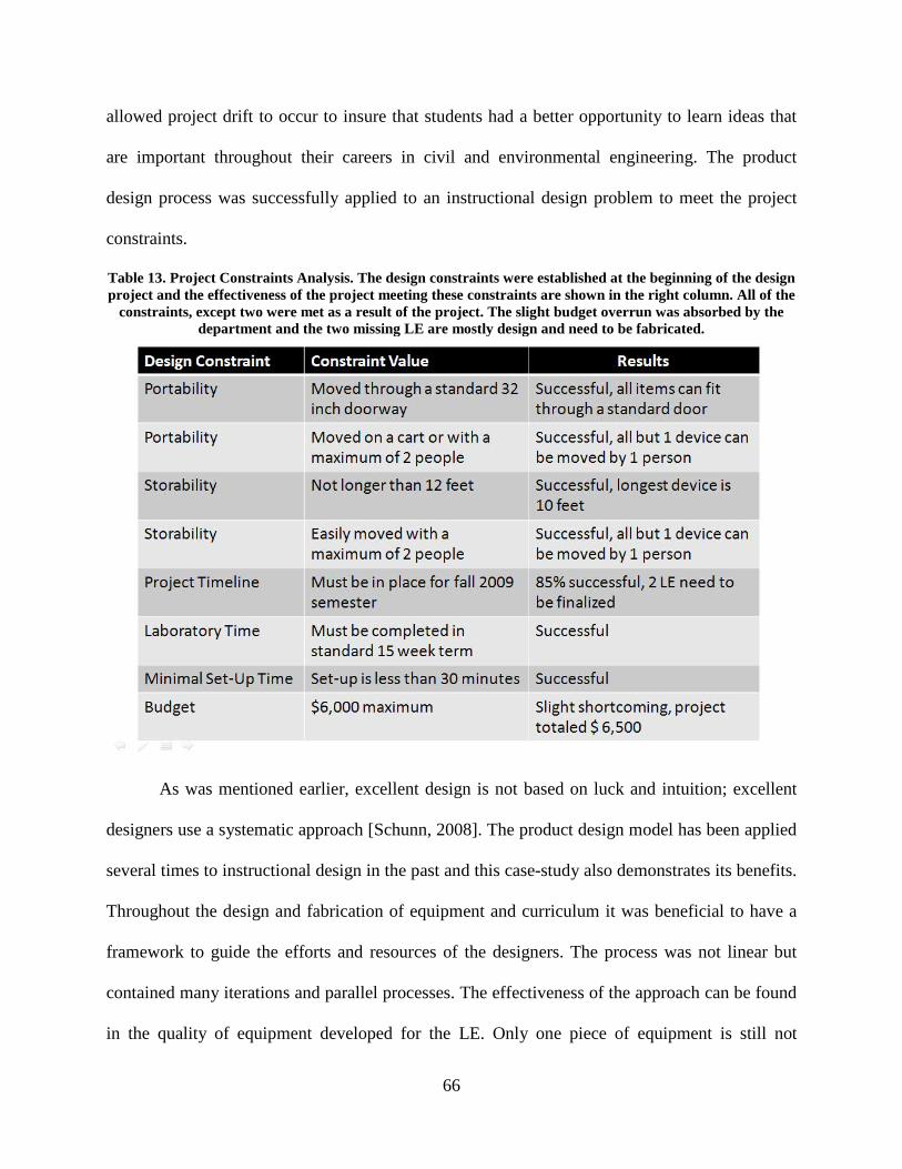
66

allowed project drift to occur to insure that students had a better opportunity to learn ideas that

are important throughout their careers in civil and environmental engineering. The product

design process was successfully applied to an instructional design problem to meet the project

constraints.

Table 13. Project Constraints Analysis. The design constraints were established at the beginning of the design project and the effectiveness of the project meeting these constraints are shown in the right column. All of the

constraints, except two were met as a result of the project. The slight budget overrun was absorbed by the department and the two missing LE are mostly design and need to be fabricated.

As was mentioned earlier, excellent design is not based on luck and intuition; excellent

designers use a systematic approach [Schunn, 2008]. The product design model has been applied

several times to instructional design in the past and this case-study also demonstrates its benefits.

Throughout the design and fabrication of equipment and curriculum it was beneficial to have a

framework to guide the efforts and resources of the designers. The process was not linear but

contained many iterations and parallel processes. The effectiveness of the approach can be found

in the quality of equipment developed for the LE. Only one piece of equipment is still not

67

working to an adequate performance level, the success rate of the prototype equipment is

amazing considering how prototypes typically require substantial revisions in order to be useful.

For instance, products that are developed using many steps in the design process are usually only

around 70% successful [Hise, 1989], any designer would be pleased with an 86% success rate.

The benefit of rapid prototyping the other curriculum for the LE was aided by the

teaching assistant being the designer. It was substantially easier to assess and utilize the feedback

in making revisions to the prototype curriculum. This benefit allowed a large amount of

curriculum to be developed in a relatively short time, some researchers report spending an entire

semester designing one LE. This project was able to develop 11 new LE and the associated

equipment in only 2 semesters.

A fundamental indicator of the effectiveness of the project is the impact on student

learning. There were two surveys developed, the results were analyzed, and the performance of

the curriculum was assessed in real-time to determine the impact on student learning.

Unfortunately, the self-assessment survey was unable to validate the project. The evaluation

survey did show that the new LE make the laboratory session less boring, improve the perception

that LE improve learning, and improve the students’ understanding of the concepts that were

covered in the LE. The test results show an initial increase in performance with a slight decrease

or leveling out that occurs once the LE were conducted in poor learning environments. The

actual gain of the new experiences on testing will most likely be higher when the LE is

conducted in a true laboratory setting. It is hard to learn when jack-hammers, dust, and the

atmosphere of an active construction site bombard one’s senses. The professor of this course also

reports that he is able to make the final harder now because students are finally getting the basic

concepts that they were unable to grasp on the first exam. This may also explain the decrease in

68

student scores. It is difficult to draw quantitative conclusions from exams that are constantly

changing. The real-time assessment of the labs showed an improvement in students’ relation of

the topics to real world situations. This is a quality that has been shown to improve learning and

the designers are very satisfied with the increased opportunity of this in the new LE. Although

some of the assessment tools were not able to provide the information that was desired, a broad

look at all of the data shows that the LE met their goal of improving student learning.

The successful redesign of the LE for any course is a difficult project. The approach of

this project was based on pre-existing concepts from product development and instructional

design. The union of the body of knowledge of these two fields is still in its infancy and few

results are described in the literature at this time. The project was successfully in developing a

new model that successfully maintained or improved student learning while creating portable

experiments. The quantitative results validate that learning was either maintained or improved.

The qualitative information shows that students are better understanding the base concepts and

this allows the instructor to utilize the additional class time to further pursue advanced concepts

with the students. The LE can successfully be designed or redesigned using the design model

described in this case study.

69

7.0 FUTURE WORK

Any major project provides the opportunity for future work and new areas to explore, this project

was no different. There are currently two LE that need to be finalized in the near future. These

LE will most likely be conducted as this thesis is reviewed and defended. The new LE should be

tested in April of 2009 and any modifications that are necessary will be made by the end of the

spring 2009 semester. The completion of these LE will completely meet all of the proposed

learning objectives and should enhance the learning experience for the students.

The self-assessment survey should be revisited to improve its performance. The terms

may be too vague for the students to accurately measure. It is recommended that the survey is

shortened and utilizes language the students will be familiar with at the completion of the course.

The current survey is long and covers all possible topics in any introductory fluids course; the

survey may create more accurate results if it is developed for typical civil and environmental

engineering fundamental of fluids courses.

Over the next few semesters it will be critical to the success of the LE that the instructor

and teaching assistant meet before each lab to discuss the next lab, and review the effectiveness

of the previous LE. The curriculum is currently effective but revisiting and evaluating the

material over the next few semesters is sure to provide opportunities for improvement.

All of the LE have only 1 piece of equipment, this makes the LE more of a demonstration

then a hands-on learning opportunity. Funding should be found to replicate the equipment in this

70

lab. It can be accomplished through reverse engineering of the devices and fabrication in the

student machine shop. These devices were all made in the student machine shop with only a few

parts requiring CNC milling that required the help of a machinist. The reverse engineering could

be a project within the CAD course in the students engineering curriculum. Student learning

outcomes should increase if all of the students are able to participate in the experiment instead of

the majority of the experience involving watching the experiments in a passive nature. The

replication of all of the labs, including data acquisition, and excluding the open channel flow

experiment would be approximately $3,000 per set. Since most labs are a maximum of 16

people, only 3 more sets would need to be developed totaling just under $10,000. With this

investment the LE would be one of the best for students in a Fundamental of Fluids course in a

civil and environmental engineering department across the country.

Finally, as the fluids laboratory space becomes available again, it would be beneficial to

develop the space as a lecture and laboratory area. The new classroom can be “L-shaped” to

allow one part of the space for lecture and another area of the room can be dedicated to

demonstrations and LE. The current course does not utilize the computer classroom that it is

taught in. There is no benefit for students to be in the computer classroom that this course is

typically taught in. Imagine discussing open-channel flow and walking around the corner to a

flume that is demonstrating the specific phenomenon that the instructor is trying to describe

through lecture. The students should benefit greatly from this type of environment. At Worcester

Polytechnic Institute they have developed a lecture/laboratory setting that is having positive

effects (Olinger, 2002). At West Point professors utilize physical models to introduce concept

topics. They believe that the model stimulates questions and leads to a dialogue as the students

learn the new concept instead of a traditional didactic approach to the introduction of theory

71

(Welch, 2007). Although the construction at Benedum may have made learning difficult for a

few semesters, it has the potential to provide the opportunity to develop a beneficial learning

environment as the new laboratory space is repopulated. It is my hope that the fluids course and

open-channel hydrology course are taught in this new facility. The components that are used to

manage flow in open-channels can easily be designed to be placed into the flume to demonstrate

most of the learning topics in the hydrology course. The students can then actually develop or

verify the concepts they are being taught in the lecture component of the course.

72

APPENDIX A

TEACHING ASSISTANT MANUAL

The manual to aid the teaching assistants in properly conducting the laboratory experiments are

on the following pages. For each LE the over-arching and content learning objectives are listed

when applicable. There is also a section with pictures of the equipment and setup instructions.

Finally there is a section that describes the intended flow of the LE, output from the data

acquisition software when applicable, and student trouble areas. The original formatting of the

training manual is retained.

73

Fundamentals of Fluids (CEE-1402)

Laboratory Experience-

Teaching Assistant Training Manual

Version 1.0

Last modified March 2009

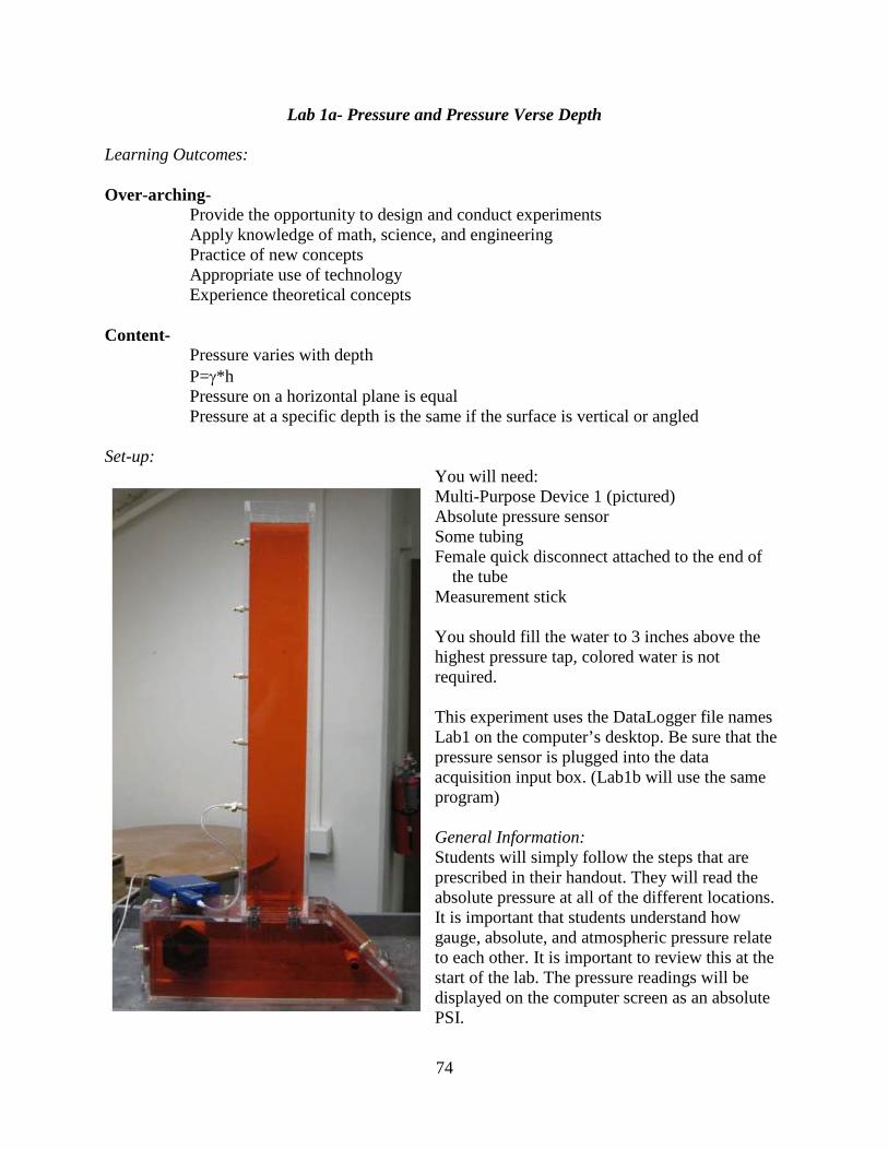
74

Lab 1a- Pressure and Pressure Verse Depth

Learning Outcomes: Over-arching- Provide the opportunity to design and conduct experiments Apply knowledge of math, science, and engineering Practice of new concepts Appropriate use of technology Experience theoretical concepts Content- Pressure varies with depth P=γ*h Pressure on a horizontal plane is equal Pressure at a specific depth is the same if the surface is vertical or angled Set-up:

You will need: Multi-Purpose Device 1 (pictured) Absolute pressure sensor Some tubing Female quick disconnect attached to the end of the tube Measurement stick You should fill the water to 3 inches above the highest pressure tap, colored water is not required. This experiment uses the DataLogger file names Lab1 on the computer’s desktop. Be sure that the pressure sensor is plugged into the data acquisition input box. (Lab1b will use the same program) General Information: Students will simply follow the steps that are prescribed in their handout. They will read the absolute pressure at all of the different locations. It is important that students understand how gauge, absolute, and atmospheric pressure relate to each other. It is important to review this at the start of the lab. The pressure readings will be displayed on the computer screen as an absolute PSI.

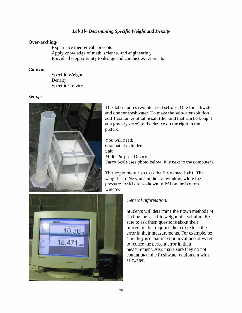
75

Lab 1b- Determining Specific Weight and Density

Over-arching- Experience theoretical concepts Apply knowledge of math, science, and engineering Provide the opportunity to design and conduct experiments Content- Specific Weight Density Specific Gravity Set-up:

This lab requires two identical set-ups. One for saltwater and one for freshwater. To make the saltwater solution add 1 container of table salt (the kind that can be bought at a grocery store) to the device on the right in the picture. You will need: Graduated cylinders Salt Multi-Purpose Device 2 Pasco Scale (see photo below, it is next to the computer) This experiment also uses the file named Lab1. The weight is in Newtons in the top window, while the pressure for lab 1a is shown in PSI on the bottom window.

General Information: Students will determine their own methods of finding the specific weight of a solution. Be sure to ask them questions about their procedure that requires them to reduce the error in their measurements. For example, be sure they use that maximum volume of water to reduce the percent error in their measurement. Also make sure they do not contaminate the freshwater equipment with saltwater.

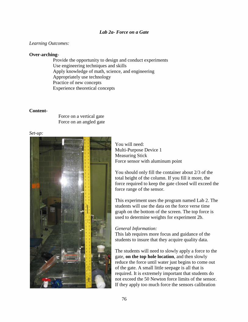
76

Lab 2a- Force on a Gate

Learning Outcomes: Over-arching- Provide the opportunity to design and conduct experiments Use engineering techniques and skills Apply knowledge of math, science, and engineering Appropriately use technology Practice of new concepts Experience theoretical concepts Content- Force on a vertical gate Force on an angled gate Set-up:

You will need: Multi-Purpose Device 1 Measuring Stick Force sensor with aluminum point You should only fill the container about 2/3 of the total height of the column. If you fill it more, the force required to keep the gate closed will exceed the force range of the sensor. This experiment uses the program named Lab 2. The students will use the data on the force verse time graph on the bottom of the screen. The top force is used to determine weights for experiment 2b. General Information: This lab requires more focus and guidance of the students to insure that they acquire quality data. The students will need to slowly apply a force to the gate, on the top hole location, and then slowly reduce the force until water just begins to come out of the gate. A small little seepage is all that is required. It is extremely important that students do not exceed the 50 Newton force limits of the sensor. If they apply too much force the sensors calibration

77

will be ruined. The computer screen below shows the output for an experiment. The students would record the minimum forces and take the average of 4 or 5 minimums. Run #2, in red, shows 9 minimums. Outliers may be removed if the student reports that he let too much water. The top reading is for experiment 2b.

Shown below is a picture of the foam on the gate. Students must accurately measure the dimensions of the area that the water exerts pressure upon. It is best to do this at the end of the experiment when a good indentation has formed on the foam; it is much easier to measure at this point.

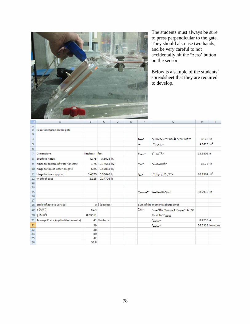
78

The students must always be sure to press perpendicular to the gate. They should also use two hands, and be very careful to not accidentally hit the “zero’ button on the sensor. Below is a sample of the students’ spreadsheet that they are required to develop.

79

Lab 2b- Buoyancy

Learning Outcomes: Over-arching- Provide the opportunity to design and conduct experiments Apply knowledge of math, science, and engineering Bridge the gap between theory and industry Practice of new concepts Exposure to real-world examples Experience theoretical concepts Content- Specific Weight Density Specific Gravity Archimedes’s Principle Buoyancy Freeboard and draft of vessels Effect of specific weight on buoyancy Set-up: There will be two identical set-ups for this experiment. One of them will have saltwater and the other is fresh water. Do not contaminant the freshwater. Use 1 container of slat, and the same

procedure you did for experiment 1b. You will need: Multi-Purpose Device 2 Graduated Cylinder Plastic “Barge” “Coal” Bee-Bee’s Aluminum Block Dial calipers Pasco Scale for weight Insure that both containers are filled to drain opening. Also, be sure to have extra saltwater available to refill the container throughout the experiment.

This experiment also uses the program called Lab2. The top window shows the weight from the Pasco scale.

80

General Information: The students should be able to follow the steps relatively easily. Students often are not careful in keeping the container completely filled; this will lead to errors in their results. You must insure that students quickly submerge the object if required. If they move too slowly they may capture some of the water that is displaced by their arms. It is very important for students to insure that their “coal” is evenly distributed along the bottom of the “barge” otherwise instability will result. The students should calculate around 2.39 Newtons of coal to keep the half inch free board, see the picture below.

81

Lab 3- Observation of Flow Patterns

Learning Outcomes: Over-arching- Provide the opportunity to design and conduct experiments Bridge the gap between theory and industry Practice of new concepts Exposure to real-world examples Experience theoretical concepts Content- Stagnation point Boundary layer Vortices/eddies Streaklines Effect of an object’s geometry on the flow of a fluid Set-up:

You will need: 1.5 bottles of Pearl Swirl (purchased form Steve Spangler, an online science education store) Flow Visualization Device Food coloring The many shapes that are shown in the picture on the next page Be sure the device is level; it has leveling knobs at its three contact points. Add a little bit of red food coloring to help visualize the flow. When the pump is running be sure the fluid level is at the height marked with the marker, see picture. If there is too much liquid the flow becomes choked, and too little fluid does not allow good visualization. Empty the contents of the device into a bucket for overnight storage. This will reduce the amount of buildup on the

bottom of the device.

82

General Information: It is very common for students to believe the shadows that result from the standing waves are the streaklines. If you explain these are standing waves and that we are interested in determining what happens to the fluid from the very beginning (when it leaves the screen) to when it flows back into the pump, students should understand better.

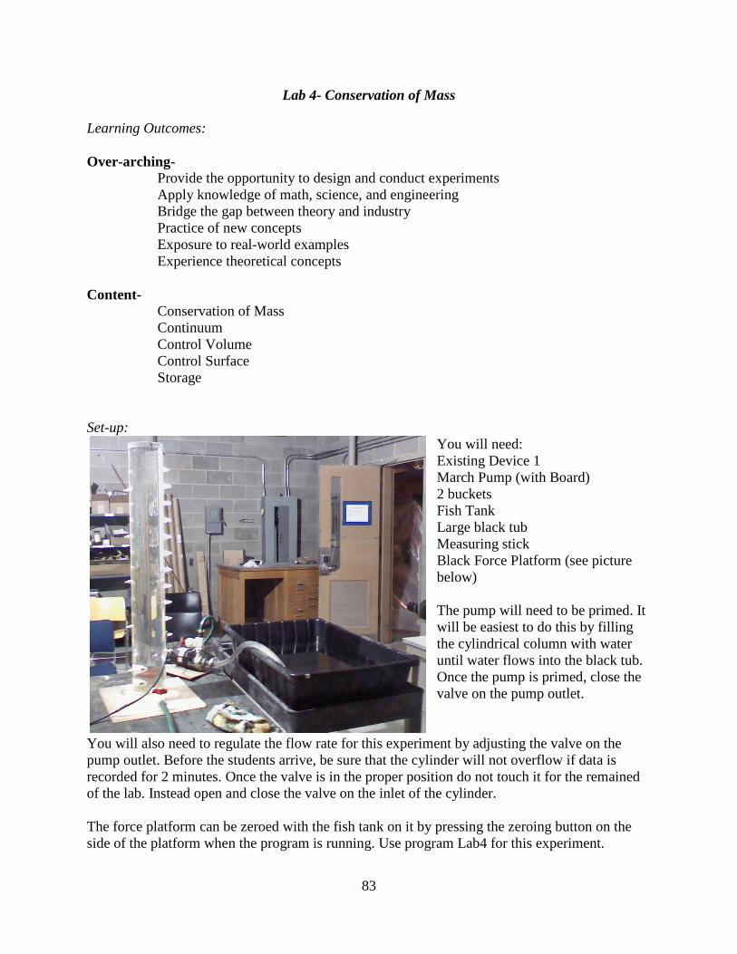
83

Lab 4- Conservation of Mass

Learning Outcomes: Over-arching- Provide the opportunity to design and conduct experiments Apply knowledge of math, science, and engineering Bridge the gap between theory and industry Practice of new concepts Exposure to real-world examples Experience theoretical concepts Content- Conservation of Mass Continuum Control Volume Control Surface Storage Set-up:

You will need: Existing Device 1 March Pump (with Board) 2 buckets Fish Tank Large black tub Measuring stick Black Force Platform (see picture below) The pump will need to be primed. It will be easiest to do this by filling the cylindrical column with water until water flows into the black tub. Once the pump is primed, close the valve on the pump outlet.

You will also need to regulate the flow rate for this experiment by adjusting the valve on the pump outlet. Before the students arrive, be sure that the cylinder will not overflow if data is recorded for 2 minutes. Once the valve is in the proper position do not touch it for the remained of the lab. Instead open and close the valve on the inlet of the cylinder. The force platform can be zeroed with the fish tank on it by pressing the zeroing button on the side of the platform when the program is running. Use program Lab4 for this experiment.

84

General Information: Students should determine a procedure that has them measuring the flow out and the change in storage. From this information they can determine the flow in. The flow out is calculated by capturing 2 minutes of low in the fish tank. The hose should be kept in the bucket until the 10 inch mark is reached. The surface when the water level is below 10 inches is too difficult to measure and this also allows the hose to completely fill with water. After the 10 inch mark is reached, the timer starts and the hose is transferred into the fish tank. The hose remains there for two minutes. Once the experiment is over, put all of the water back into the black tub. The change in storage is determined by measuring the change in height for the two minutes.

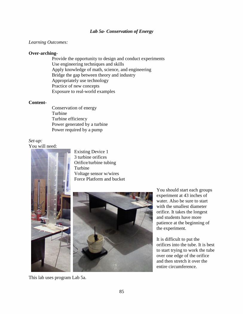
85

Lab 5a- Conservation of Energy

Learning Outcomes: Over-arching- Provide the opportunity to design and conduct experiments Use engineering techniques and skills Apply knowledge of math, science, and engineering Bridge the gap between theory and industry Appropriately use technology Practice of new concepts Exposure to real-world examples Content- Conservation of energy Turbine Turbine efficiency Power generated by a turbine Power required by a pump Set-up: You will need:

Existing Device 1 3 turbine orifices Orifice/turbine tubing Turbine Voltage sensor w/wires Force Platform and bucket

You should start each groups experiment at 43 inches of water. Also be sure to start with the smallest diameter orifice. It takes the longest and students have more patience at the beginning of the experiment. It is difficult to put the orifices into the tube. It is best to start trying to work the tube over one edge of the orifice and then stretch it over the entire circumference.

This lab uses program Lab 5a.

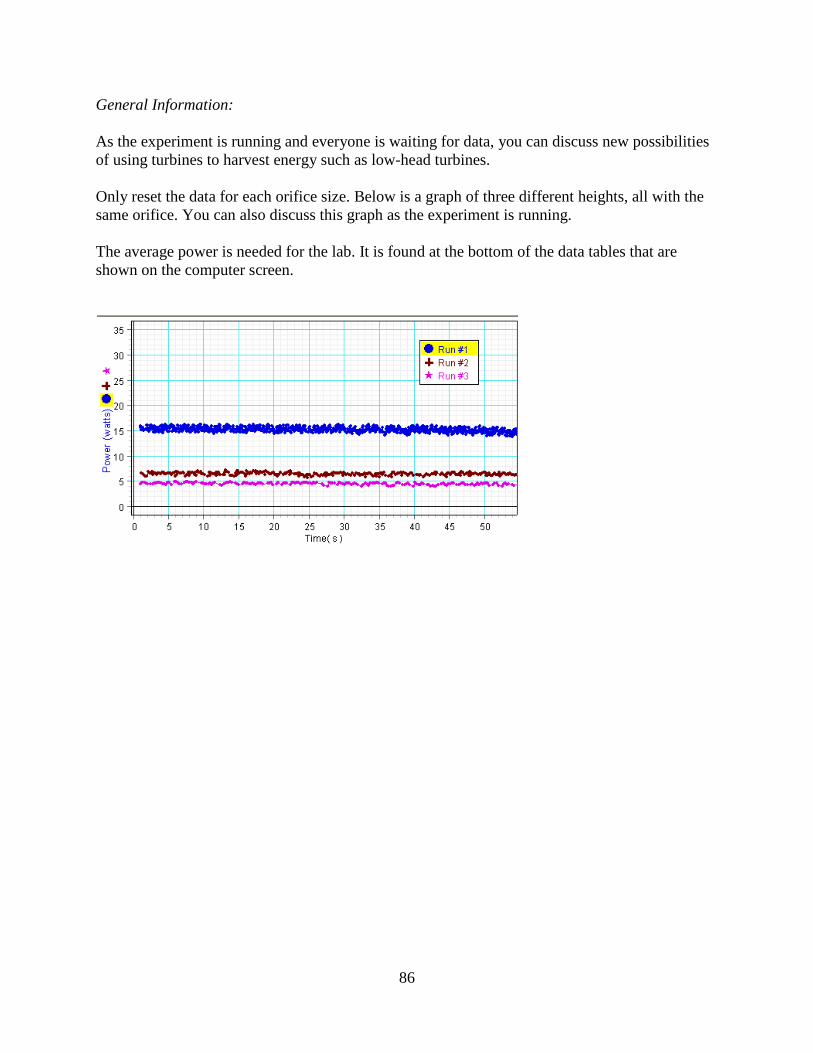
86

General Information: As the experiment is running and everyone is waiting for data, you can discuss new possibilities of using turbines to harvest energy such as low-head turbines. Only reset the data for each orifice size. Below is a graph of three different heights, all with the same orifice. You can also discuss this graph as the experiment is running. The average power is needed for the lab. It is found at the bottom of the data tables that are shown on the computer screen.

87

Lab 5b- Conservation of Momentum

Learning Outcomes: Over-arching- Provide the opportunity to design and conduct experiments Apply knowledge of math, science, and engineering Bridge the gap between theory and industry Appropriately use technology Practice of new concepts Exposure to real-world examples Experience theoretical concepts Content- Conservation of momentum F=P*A Reaction forces for pipe fittings Set-up:

You will need: Unique Device 1 Both pumps connected in series (need as much pressure as possible) Absolute pressure sensor Fish tank Bucket Force Platform (not pictured) Fill the fish tank with water before you prime the pump. It is easiest to prime the pump by filling the outlet hose full of water and open both valves. Once it is primed close one of the valves to keep it primed. This experiment uses the program called Lab 5b. Insure that the fitting is pressed against the force sensor and then zero the force gauge (the data software must be running). Also be sure the 180 degree bend is centered on the force gauge.

88

General Information: The flow rate in the lab should be controlled by the second pumps valve. The first pump should always run completely open. Use the flow rate gauge only to get an idea of how the flow is being adjusted. Always be sure students weigh the amount of water that comes out in a specific time to determine the flow rate in the pipe. The pressure sensor always needs to be connected. If the reading is atmospheric, the pipe is not running full and the experiment is over. Review how to determine gauge pressure from atmospheric and absolute pressure.

89

Lab 6- Piping Lab

Learning Outcomes: Over-arching- Provide the opportunity to design and conduct experiments Apply knowledge of math, science, and engineering Bridge the gap between theory and industry Appropriately use technology Practice of new concepts Exposure to real-world examples Experience theoretical concepts Content- Conservation of energy Head loss in a pipe Head loss in a fitting Head loss in various valves Equivalent length of pipe Determining K (loss coefficient) Moody Diagram Set-up:

You will need: Multi-Purpose Device 3 Check valve Gate valve Globe valve Ball valve Fish tank Bucket Force platform Absolute pressure sensor March Pump (with wood base) 2 wrenches Tape measure or measuring stick The pump will need to be primed. It is easiest to prime by pouring water into the suction end with the valve open after the pump. Once, it is primed close the valve.

This experiment uses program Lab6 on the computer.

90

The fish tank is used for the pump suction house to draw from; the bucket is used to catch a certain amount of water for a given time. The device can be used as shown in the picture to the left, just be sure the valve is closed so water does not come out of the black fitting in the picture. It is very easy to just connect the pump into the system without the tee, but it is not required, it would increase the flow rate and thus the head loss. General Information: Students will follow the direction in the lab hand-out. Help them to properly loosen the unions on the copper pipes when required. It is important to keep the pipe form spinning with one

wrench while the nut is loosened with another wrench. This will keep the system from forming a leak. There are valves in the storage area that are already loosened that students can take a part to see how the inside of the valves are designed. This should help them understand why one valve is substantially better or worse than another valve. Below are the different valves in the lab. Form the top:

Ball valve- usually has a lever handle Check valve Globe valve- a more spherical valve body Gate valve- a more rectangular valve body

91

Lab 7- Pump Lab

Learning Outcomes: Over-arching- Provide the opportunity to design and conduct experiments Use engineering techniques and skills Apply knowledge of math, science, and engineering Bridge the gap between theory and industry Appropriately use technology Practice of new concepts Exposure to real-world examples Experience theoretical concepts Content- Relationship between pump head and flow rate Creating pump performance curves: Single pump Pumps in parallel Pumps in series Set-up:

You will need: Multi-Purpose Device 3 Fish tank Bucket Force platform Absolute pressure sensor Both Pumps Flat blade screwdriver 2Wrenches The pump will need to be primed. It is easiest to prime by pouring water into the suction end with the valve open after the pump. Once, it is primed close the valve. This experiment uses program Lab6 on the computer.

The fish tank is used for the pump suction house to draw from; the bucket is used to catch a certain amount of water for a given time.

92

To make the lab flow quicker, connect both pumps up to the system before the start of the lab. Both suction hoses can be placed in the fish tank. Control the ball valves on the tee to determine which pump is to be tested, or for the pumps to run in parallel. You will need to unattach one of the houses form the tee and close the valve on that side when the pumps are connected in series. Pumps in series have the output of one pump flowing into the suction of another pump. General Information: Students follow the procedure in the lab hand-out. Be sure that all of the valves are in the proper position before the pumps are started each time so water does not go where it is not intended. Close the pump valves completely before turning off the pumps so that the pumps do not need to be re-primed.

93

Lab 8- Open Channel Flow

Learning Outcomes: Over-arching- Provide the opportunity to design and conduct experiments Use engineering techniques and skills Apply knowledge of math, science, and engineering Bridge the gap between theory and industry Practice of new concepts Exposure to real-world examples Experience theoretical concepts Content- Olgee Spillway Critical depth Froude Number Hydraulic jump Energy loss in hydraulics Set-up:

You will need: Unique Device 2 Hoses Large reservoir Large pump Pump controller Bucket Force Platform Rulers Completely fill the reservoir tank, this will provide enough water for the experiment. Practice creating a hydraulic jump before the lab by adjusting the gate

at the outlet of the flume. Usually you must close it a bit to create the jump, and then open it more to stop the jump from moving upstream. The pump is a variable speed. Turn the controller on, press the PU button. Adjust the drive frequency by rotating the knob to the desired value; 30 Hz is sufficient for this lab. Once you have the proper value press set. This experiment uses the program named Lab 8 on the computer.

94

General Information: The students will follow the lab hand-out for this experiment. Be sure that students get the proper critical depth on the spillway. Also be sure that they are measuring the hydraulic jump as effectively as possible.

The velocity measurement device that uses the propeller should be used midway between the spillway and the entrance to the flume to get the best measurements.

95

Lab 9- Measurements in Fluid Mechanics

Learning Outcomes: Currently Being Developed

Over-arching- Provide the opportunity to design and conduct experiments Use engineering techniques and skills Apply knowledge of math, science, and engineering Bridge the gap between theory and industry Appropriately use technology Practice of new concepts Exposure to real-world examples Experience theoretical concepts Content- Pitot Tube to measure velocity Orifice plate to measure velocity Venturi Meter to measure velocity Applications of Bernoulli’s Equation Applications of conservation of energy Set-up: General Information:

96

Lab 10- Reynolds Lab and Moody Diagram

Currently Being Developed

Learning Outcomes: Over-arching- Provide the opportunity to design and conduct experiments Use engineering techniques and skills Apply knowledge of math, science, and engineering Appropriately use technology Practice of new concepts Experience theoretical concepts Content- Reynolds Number Turbulent flow Laminar flow Moody Diagram Head loss Set-up: General Information:

97

APPENDIX B

LABORATORY EXPEREINCE HANDOUTS

The handouts that are provided to the students for each LE follow on the subsequent pages. They

are in chronological order as the students would experience them throughout the semester and

follow this page. They are also placed in this document without headings to maintain the

formatting of the handouts.

98

CEE 1402 FLUID MECHANICS LABORATORY

Experiment 1a: Pressure at various points

Objectives: The purpose of this lab is to visualize and thoroughly understand the pressure at various points in a system:

• Pressure with depth varying • Pressure on a horizontal plane • Pressure on a vertical surface vs. an angled surface

Procedure and Analysis:

1. Fill the device with water just below the top of the water column. 2. Record the pressure that the pressure sensor displays when it is only measuring atmospheric pressure. Pressure with depth varying(p1, p2, …, pn, h) Measure the depth of each pressure tap ( note reading is atmospheric pressure + inches of water) 3. Use the pressure sensor to obtain the pressure at each location, record your results. This value is the absolute pressure. 4. Repeat the experiment 2 times obtain three total pressure data sets

• Plot the data of pressure (pounds/feet2) vs. depth (feet) Write-up

• Use excel or other methods to determine the slope of the best fit line for this data • Subtract the atmospheric pressure from each data point for pressure, re-plot the data, and find the slope of the best fit line • Discuss how the value of the slope of the lines compares to the specific weight found in the back of the book. Also explain why each graph has a different y-intercept. • In the above experiment we have measured or calculated the gauge pressure, atmospheric pressure, and absolute pressure. In your own words describe each one of these as it relates to our experiment.

Pressure on a plane (p1, p2, p3, h) 5. Record the pressure for each of the 3 pressure taps on the horizontal surface of the box

• Using your data either prove or disprove the following statement. Pressure on a horizontal plane in a static fluid is constant.

Write-up

99

Pressure on a vertical surface verse an angled surface (p1, p2, h) 6. Record the pressure at the pressure tap on the bottom vertical surface, also record the depth of this pressure tap 7. Record the pressure at the pressure tap on the angled surface, also record the depth of the pressure tap

• Discuss the comparison of these two data points after you convert them to gauge pressure with the pressure expected at this depth using Pressure (p) = g*depth (h). Be sure to watch your units!

Write-up

• From your data above and previous experiments does this prove or disprove the following statement. Pressure on a horizontal plane in a static fluid is constant regardless of the angle of the surface to the water.

100

Experiment 1b: Determining Specific Weight

Objectives: The purpose of this lab is to develop a method to measure the specific weight of a fluid. Procedure and Analysis: Using a graduate cylinder, computer weight scale, water, and salt water determine the specific weight of each solution. PLEASE ONLY USE SALT WATER IN THE CONTAINERS LABELED SALT WATER!

• Clearly list the steps of your experiment Write-up

• Calculate γ (gamma-specific weight) and S (specific gravity) of each solution. Assume the water temperature is 60 degrees. You will need to reference the table in the back of your book.

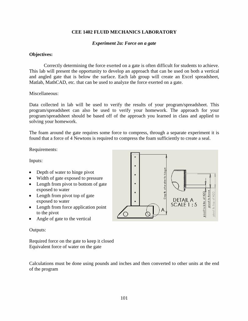
101

CEE 1402 FLUID MECHANICS LABORATORY

Experiment 2a: Force on a gate

Objectives: Correctly determining the force exerted on a gate is often difficult for students to achieve. This lab will present the opportunity to develop an approach that can be used on both a vertical and angled gate that is below the surface. Each lab group will create an Excel spreadsheet, Matlab, MathCAD, etc. that can be used to analyze the force exerted on a gate. Miscellaneous: Data collected in lab will be used to verify the results of your program/spreadsheet. This program/spreadsheet can also be used to verify your homework. The approach for your program/spreadsheet should be based off of the approach you learned in class and applied to solving your homework. The foam around the gate requires some force to compress, through a separate experiment it is found that a force of 4 Newtons is required to compress the foam sufficiently to create a seal. Requirements:

Inputs:

• Depth of water to hinge pivot • Width of gate exposed to pressure • Length from pivot to bottom of gate

exposed to water • Length from pivot top of gate

exposed to water • Length from force application point

to the pivot • Angle of gate to the vertical Outputs:

Required force on the gate to keep it closed Equivalent force of water on the gate

Calculations must be done using pounds and inches and then converted to other units at the end of the program

102

Write-up: (A complete lab report is not necessary for this section)

Comparison of the program results verse the lab results, with a discussion about the differences appropriate diagrams, variables, and equations must be included to clearly communicate the method that your program utilizes to perform the required calculations. The computer file and output for the vertical and angled gate must be emailed to the teaching assistant. Extra credit is available if your program is verified by solving a homework problem, the amount of extra credit is dependent upon how well you communicate the verification

103

Experiment 2b: Buoyancy Lab

Objectives: The purpose of this lab is to understand several more basic properties of fluids and their application:

• Density • Archimedes’s Principle • Freeboard and draft related to transportation of goods using barges

Procedure and Analysis:

• The first two parts of this lab will be conducted twice, once using normal tap water and another time using saltwater. • DO NOT PUT SALTWATER INTO THE FRESHWATER TANK AND VICE VERSA. • All write-ups will be done for both regular and saltwater.

Density

1. Fill the device with water so that water just begins to come out of the side tube 2. Measure the volume of the solid aluminum block using a ruler 3. Gently but quickly place the object into the container and capture the amount of water that flows out of the container. Do not drop the block 4. Measure both the volume and the mass of this water 5. Refill the water in the container so it just begins to come out of the tap

Write-up (show all calculations)- • What is the volume of the aluminum block? What is the volume of water that left the container? How do the two values compare? • What is the weight of the aluminum block? How does it compare to the weight of the water that left the container? • What is the density and specific weight of aluminum? • What is the density and specific weight of the water?

Archimedes’s Principle

6. Insure that the water level is such that water just begins to come out of the container 7. Measure the weight of the barge using the scale, you may have to convert units 8. Measure the cross-sectional area that would represent the length and width of the barge 9. Place the boat into the water and measure the weight and volume of the water that flows out of the container, DO THIS STEP BEFORE STEP 9 10. Measure the depth that the barge sinks in the water, if you push the barge towards the side of the container it will be easier to measure. This is the draft of the barge when it is empty 11. Refill the water in the container so it just begins to come out of the tap 12. Use the dial calipers to determine the volume of plastic that is used in the barge.

104

13. Quickly sink the barge by putting it into the water on its side and measure the volume of water that flows out of the container 14. Refill the water in the container so it just begins to come out of the tap 15. Repeat steps 1-13 but use saltwater.

Write-up (show all calculations)- • What is the weight of the barge? What is the weight of the water displaced by the barge? How do these two values compare? Explain how this supports or disproves Archimedes’s principle found on page 61 of your textbook? • What is the volume of the barge that is submerged? What is the volume of the water displaced? How do these values compare? • What is the density and specific weight of the plastic that makes up the barge? • How do the values for step 10 and 11 compare? Discuss your results and any errors that may have occurred. • Create a free body diagram for the barge and for the block. Applying Archimedes’s principle what is the buoyancy force exerted on the barge? What is the buoyancy force exerted on the block? Provide the values for all of the forces that act on the barge and the block, remember that the objects are stationary so the forces must sum to zero according to Newton’s Second Law.

THIS EXPERIEMNT IS ONLY DONE IN FRESHWATER, NOT SALTWATER Freeboard and Draft As mentioned earlier the draft is the amount of the boat that is below the surface of the water. The U.S. Army Corps of Engineers guarantees the depth of the Monongahela to be at least 9 feet. This is accomplished through locks, dams, reservoirs, and reservoir releases. The entire system is very interesting and more can be learned about this system by taking the Water Resources course. When circumstances require, The Corp of Engineers has the ability to send surges down the river to allow “special” transportation depths up to 11 feet. The next section of the lab is an application of basic knowledge about fluids and design. The Problem- You work for a major regional coal company and need to optimize the amount of coal that can be transported up the Monongahela using the barges that your company has already purchased. These barges where specially designed so that their draft will be the maximum draft allowable for river travel when they are fully loaded. When a barge is fully loaded it still has a certain amount above the water to prevent waves from entering the cargo area. The amount above the water is known as freeboard. You have developed a scale model to determine what the maximum load the barge can carry while maintain the minimum freeboard. What is the maximum amount of weight that your model barge can carry in freshwater while still maintain a ½ inch freeboard? Experiment- Be sure to completely measure all aspects of the barge so that you can complete the problem. You will add bee-bee’s to your barge to represent coal. Determine how much “coal” your barge can carry and still maintain a ½ inch freeboard. (92 bee-bee’s = 42 grams)

105

Once you have calculated the weight of bee-bee’s that your barge can carry, you will verify your results by actually conducting the experiment. Put your estimated number of bee-bee's into the freshwater barge and place it into the freshwater tank. How much freeboard remains? Write-up-

• Clearly show all of your calculations to determine the amount of “coal” your barge can carry. • Discuss how well your calculated value compared to the result from the lab. • What would be the mass of coal that could be carried if these barges were used in saltwater (the same saltwater in our lab)? Assume that the freeboard remains constant at .5 inches, this is a poor assumption but it will help reinforce concepts in this lab, why is this a poor assumption?

Final Questions-

• In the first two parts of this lab, density and Archimedes’s Principle, we conducted the experiment in both saltwater and freshwater. Compare the weight/mass and volume of water that left the container when it was fresh and saltwater for the barge and also for the block (it may be useful to create a table with the weight and volume of water that left the container for the barge floating and sunk as well as the aluminum block, include your calculated buoyancy forces as well). Also, how does the weight of water that left compare to the buoyancy force? Justify why they were the same or different. • Put Archimedes’s Principle in your own words, and relate it to the data from the laboratory experience.

106

CEE 1402 FLUID MECHANICS LABORATORY Experiment 3: Observation of Flow Patterns

Objectives:

A study of flow patterns is often needed in the design of fluid mechanics or hydraulic systems. The objective of this experiment is to observe the streaklines around objects of different geometrical forms in a flow-visualization channel. The streaklines will be shown by a material that is suspended in the water, it is called Pearl Swirl. Do not be confused by the standing waves that will form around the object, these will appear as dark shadows as you look at the water, this does not represent the flow of the fluid. At the conclusion of this lab you should understand the following:

• stagnation point • boundary layer • vortices/eddies • streaklines

Procedure and Analysis:

1. Fill the experiment apparatus with water until the channel is approximately half inch deep. 2. Move the apparatus until it is on level ground, within reach of an electrical outlet. Plug into the wall and flip the switch so the pump starts and water begins to flow. 3. Add the Pearl Swirl concentrate, 1.5 bottles should be sufficient. 4. Place the following objects in the narrow channel and clearly draw the flow patterns, you must show the following if applicable:

• stagnation point • vortices/eddies • 3-5 streaklines

Objects:

• Rectangular piece- this is the simplest form for concrete and hence bridge piers • Round piece- a simpler form for concrete

The above objects have disadvantages that engineers have been able to reduce. The next few objects will show the progression from the above objects to the ideal shape for an object that is placed in a flow stream.

5. Place the following objects in the narrow channel and clearly draw the flow patterns, you must show the following if applicable:

Objects: • rectangular piece with a half cylinder in front • rectangular piece with a half cylinder in front and in back • airfoil (half-cylinder piece in the front, triangle piece behind)

107

More than one bridge pier is usually placed in a stream or river. Use the 3 cylinders to represent 3 bridge piers going across the stream; it may be necessary to hold them in place. Note what happens to the water level by looking at the side of the water channel. Sketch this profile

. Later in the semester we will be learning about this phenomenon, you should see that a choke point occurs, these cause negative effects to open-channel waterways. Choke points raise the water level before the obstruction and also cause increased stream velocity below the obstruction. Why would these be negative effects?

We have two Matchbox cars, using what you have learned predict what the flow patterns around each car would look like. Show these to your instructor and then place the cars back into the flow stream and draw the following:

Checking in (before you leave):

• stagnation point • vortices/eddies • 3-5 streaklines

Write-up (per lab group):

1. In your own words define/describe the following based off of what you learned in this lab, from class, the textbook, or other sources:

• stagnation point • boundary layer • vortices/eddies • streaklines

2. Clear drawings of each object placed in the flow stream.

3. The half cylinders improved the flow patterns around the rectangle. What does each half cylinder do to improve the flow?

4. It can be seen from the lab that the airfoil has the best flow pattern, please discuss why this shape is not used for bridge piers; you should have several answers for this. You should utilize general knowledge as well as knowledge from other classes.

108

CEE 1402 FLUID MECHANICS LABORATORY

Experiment 4- Being a Dam Engineer

Dam Engineers have many dam responsibilities. A dam engineer who works at a reservoir must be sure that their dam will not overtop. Overtopping occurs when the water level raises above the design limits of the dam and water flows overtop of the dam. This is a primary cause of dam failures around the world. If you become a dam engineer, or you design dams you must understand and be able to apply the concept of Conservation of Mass.

This lab is a model of a reservoir system. The reservoir is the tall plastic cylinder. A reservoir is responsible for storing water that falls on its watershed. Watersheds are the land area that will drain to a specific point, in this case, the reservoir. When rain falls, some of the water is absorbed into the soil, but a substantial part can turn into runoff and flow through the watershed to a reservoir. The inlet valve from the building water supply represents the runoff for the watershed we are concerned with. As dams are designed the engineer must determine what the max rainfall and thus, the max runoff will be. The valve has been preset to allow a specific amount of “runoff” for our lab; this is the worst case rainfall and storm our dam will be designed to.

Another reservoir design choice is outflow. This is often controlled be gates that are built into a dam. A dam engineer will need to know when to open or close these controls to maintain the proper reservoir level as well as control the flow and water level of the outlet water. In our lab we will simulate this by controlling the valve on the outlet of the cylinder.

109

Conservation of Mass: If we choose our control volume to be a cylinder below the surface of the water in the reservoir (column) the flow inside the control volume is steady, therefore the first integral will go to zero.

The second integral will simplify to: ρ1*A1*n V1 + ρ2*A2*n V2 + ρ3*A3*n V3 = 0 1= inlet surface 2= control surface below water level in cylinder 3= outlet surface ρ1 = ρ2 = ρ3, therefore the above equation simplifies to: A1*n V1 + A2*n V2 + A3*n V3 = 0 n is a vector that points away from the control volume, therefore some of the above terms will be negative when the dot product is taken between n and V (velocity). In our lab we will not be able to measure velocity or area, and most dam engineers are not concerned with velocity nearly as much as flow (Q). Q=A*V Therefore, combining the 2 previous equations: Q1 +Q2 +Q3 = 0 However, in our lab we will not be measuring area or velocity, but we will measure the total volume.

This approach will be useful for determining the mass that is passing through the outlet control surface, or through the “gates of the dam”. Dam engineers are always concerned with the rate that the reservoir is raising. We will measure this information as well in our lab. The rate of rise (dh/dt) would be the velocity of the fluid through the second control surface.

c.v.

=Q*∆t

110

Experiment 1 (as a class): There is a massive rainfall and the runoff is filling up your reservoir. Using indirect measurements determine the flow thru each control surface (inlet, just below reservoir water level, outlet). For our experiment we will only “fill” the reservoir for 2 minutes. We will start the experiment when the water level is at 10 inches. Information that may be useful: Diameter of cylinder Volume of water in fish tank after 2 minutes Change in height over the two minutes Experiment 2 (individual lab groups): The massive storm continues (assume the flow into the reservoir is the same as Experiment 1) but you have a dam problem. One of your gates has broken. It was poorly designed and has failed in the closed position; you now have a decreased flow out of the reservoir. How long after the experiment beings will the reservoir overtop? How tall would our cylinder have to be if it would take 20 minutes for the gate to be repaired? Note: We will only run this experiment for 1 minute; again start the experiment when the water level reaches 10 inches. More information that may be useful to collect: Volume of water in fish tank after 1 minute Change in height over 1 minute Height of cylinder above starting water level

111

CEE 1402 FLUID MECHANICS LABORATORY

Lab 5- Energy and Momentum

5a- Turbines

Engineers and society are looking at turbines as a source of generating renewable energy more and more. After a turbine system is optimized it can have an efficiency of 90+ %. This is in stark contrast to a coal-fired power plant that is approximately 35%. Key factors in optimization are flow rate and head. Each turbine is designed to operate most efficiently on a narrow range of these factors. It is your job today to determine what the best design parameters for our turbine are, a much smaller scale than one used at a hydro-electric dam. Objectives: To apply the energy equation to a turbine and determine the effects of

parameters on efficiency

Energy Equation applied to Turbines

The energy equation for steady uniform flow is: Hp + V12/(2g) + P1/γ + z1 = HT + V22/(2g) + P2/γ + z2 + hl (1) Point 1 is located at the top of the water surface in the column. Point 2 is located at the point that the water hits the turbine. Therefore, we will assume that the water stops when it hits the turbine and V2=0. We will set our coordinate access at Point 2, therefore z2 =0. Since the water column and the stream of water are both in the atmosphere, there pressure = 0 as well. The velocity of the fluid at Point 1 is also very small when compared to Point 2, therefore V1 = 0. We do not have a pump involved so Hp=0. We will also assume there is no head loss. This assumption will cause the efficiency of the turbine to be lower.

The energy equation can now be rewritten as: z1 = HT (2) We also know that the power generated by a turbine with an efficiency ηT is: WT = γQHT ηT (3)

112

In our experiment we will record the average power over a given time period. We will also need to know the average flow rate and the average value of z1. Our goal will be to determine what will make the turbine work most efficiently. We will vary the z1 and also the orifice diameter. Procedure:

1. Determine how far above Point 2 the top of the acrylic sheet is. This will be where we make all of our measurements from. Use the clear plastic tube and the concept that water will be at the same level in the tube to help you make accurate measurements.

2. Place the smallest orifice into the tube and position it into the turbine so that it is as close to the blades but does not interfere with the movement of the blades.

3. Fill the water column very close to the top. 4. Open the valve for the turbine. Begin the experiment when the water level passes

a specific inch mark on the measuring stick. You begin the experiment by pressing start on the program.

5. The program will record the time and average power over the duration of the experiment. Stop the experiment after 2 inches of water has left the cylinder; remember the cylinder has a diameter of 5.5 inches. The average height will be used in the calculations that you perform later.

6. Record the total time of the experiment, the beginning and ending heights (this will be used to find the average height that you will use in equation 2), and the average power in watts.

7. Close the valve to the turbine and open the valve to the drain hose, let the column drain to about 2/3 of the total height, then close the drain hose.

8. Repeat steps 4-6. 9. Close the valve to the turbine and open the valve to the yellow drain hose, let the

column drain to about 1/3 of the total height, then close the drain hose. 10. Repeat steps 4-6. 11. Now you will switch to a different orifice. Carefully remove the smallest orifice

and replace it with the medium sized orifice. Be sure that when you place it back into the turbine you get it as close to the blades as possible without interfering with them.

12. Repeat steps 3-10 13. Now you will switch to the last orifice. Carefully remove the medium orifice and

replace it with the largest orifice. Be sure that when you place it back into the turbine you get it as close to the blades as possible without interfering with them.

14. Repeat steps 3-10

113

Write-up

1. Make a sketch of the experiment that clearly shows all relevant measurements. 2. Create an orderly table of the data your recoded. Include the efficiency, Q,

average z1, power, and total energy produced for each of the nine variations we performed for the experiment. Assume the water is at 60 º F. The diameters of the orifices are: .060 inches .205 inches .319 inches

3. Discuss what would be the optimal design and why. 4. If we assume that the loss coefficient in the pipeline (including entrance and exit

losses) to be K=1.5, what is the actual efficiency of the turbine? Explain why it changes.

5. Students are trying to determine if they can generate any substantial electricity by capturing the rainwater that falls on the roof of Benedum and using it to generate electricity. The group will use the turbine that you have used in the lab. Is this a useful endeavor? Explain.

You will need to find out some information to arrive at your conclusion, below are some suggested points to consider:

• Height of Benedum Hall • Where the turbine will be located • Average rainfall (monthly/yearly totals)

6. As our society becomes more aware of our impacts of everyday life on the

environment there are suggestions for how we can live “greener” in our everyday. One of these suggestions is that we should only take 5 minute showers and uses a low-flow shower head. Of course, some of you may be motivated to save the environment by not showering for days at a time. How much energy (in Joules and kW*h) is required by a pump if it is running at an efficiency of 85% to supply the water to your shower for an entire year if you take “green” showers. Assume there is no headloss in the system (bad assumption but it will make the problem easier), the flow through the shower head is 1.75 gpm, the water is pumped from the water treatment facility reservoir on the Allegheny river which has an approximate elevation of 850 feet, to your bathroom which is approximately 1300 feet, assume you shower every day, and assume the pressure as the water reaches the shower head is 30 PSI. How does this compare to a normal American who spends 8 minutes in the shower and uses a shower head that has a flow rate of 2.6 gpm.

114

5b- Momentum Objectives: To determine the reaction force of a 180º turn in a piping system

To develop a force characteristic curve for 180º turns The moment equation is: ∑Fx=m*(V2x-V1x) (1) ∑Fy=m*(V2y-V1y) (2) ∑Fz=m*(V2z-V1z) (3) Where the x-axis points in the direction of flow into the turn, the y-axis is perpendicular to the x-axis, and the z-axis points straight up from the mounting surface. In our lab we will only be concerned with equation (1). For discussion we will only work with equation (1) for a 180 º turn. Expanding (1) in this situation yields: p1A1-Rx+p2A2=m*(V2x-V1x) (4) Since the pipe vents to the atmosphere p2=0, and m= ρQ= ρAV, V2x=-V1x , and V =|V1x| (4) simplifies to: p1A1-Rx= -2ρAV2 (5) Rx= 2ρAV2 + p1A1 (6) Rx= 2mV + p1A1 (7) In lab we will be able to measure Rx directly and V indirectly based off of the flow. We may also choose to just determine the mass flow rate. The pressure in the pipe will be measured in p.s.i., you will need to convert to feet of water. Procedure:

1. Completely open the valve by the pump; Let the system stabilize and adjust the fitting so it is centered on the rubber force probes.

2. Record data for 10 seconds using the computer. Record the average reaction forces, the flow rate, the pressure, and the mass of water that flows in 10 seconds.

3. Decrease the flow by about 2 gpm and repeat step 2. 4. Continue repeating step 3 until you reach 2 gallons per minute.

115

Write-up

7. Create a table that clearly shows all of the data collected as well as the pressure. Also include derivations, unit conversions, and equations you used to determine the calculated reaction force. You need to calculate the reaction force based off of the mass flow rate and the flow rate determined by the flow meter. (There will be errors in these measurements).

8. Clearly compare and discuss your computed force reaction results with the actual values recorded in the lab. Which measurement method is more accurate? Where do errors occur? etc.

9. You will find that the reaction force is very small, .5” copper pipe is common, or even a small size for residential homes. Since the reaction forces are so low excessive care is not required to accommodate these forces. However, in large scale applications such as pump stations or hydro-electric dams the reaction force needs to be accommodated in the facility design. Later in the course you will use pump characteristic curves. You will also find, in your careers, that characteristics curves can be used to approximate many values. To understand how these are created, please create a Reaction characteristic curve for the 180º turn. Follow the following guidelines for success:

a. The graph should have the reaction force on the y-axis b. The x-axis should have the flow in gallons per minute c. Create the graph with the average pressure of 60 psi, and with the water

temperature at 60 º F. d. There should be separate curves for different pipe diameters, start your

pipe diameters at 16 inches and go up from there in standard sizes for cast iron pipe (a common pipe material in water distribution systems). You should have at least 6 different standard pipe diameters.

e. Choose your range of values for flow to be in the range of 0 to 130 cfs. An example of a characteristic curve can be found on page 612 Figure 12.6 of your textbook.

116

CEE 1402 FLUID MECHANICS LABORATORY

Lab 6- Piping Systems Overview: No matter what specialty of Civil and Environmental Engineering you choose you will most likely have to determine the losses in a piping system to help you select the proper pump. In this lab we will examine the head losses in a piping system; in the next lab you will develop pumping systems. Combined you should be able to properly select a pump(s) for a given piping system. You will need to reference and understand Section 7.6 in your textbook.

Procedure and Analysis:

1. Insure that the pump is properly primed; your instructor will help with this. 2. Record the atmospheric pressure of the room before starting the experiment; you will

need this to determine gauge pressure since our reading is in absolute pressure. 3. Draw a sketch of the piping system. Include actual dimensions, the pump, valves, and

pressure tap locations. Use proper symbols in your final write-up. 4. Assume the water temperature is 65 degrees Fahrenheit

***Write-up • Provide a sketch of the piping system with the actual dimensions, pump, valves, and

pressure locations clearly and properly shown Part A- Pressure losses in a length of pipe and equivalent length

5. Be sure the container on the scale is empty and close the valves on the section of the pipe network that contains the cooper pipe

6. Turn the pump on and completely open the valve closest to the pump 7. Record the pressure at pressure tap location 2-6 8. Determine the flow rate

***Write-up • Calculate the flow rate • Report the pressure drops in a table for this piping system, you should have pressure

drops measurements with the following pairings: 2 and 6 5 and 6 4 and 5 3 and 5

• Using the flow rate, moody diagram and Table 7.2 determine what the calculated pressure drops should be for each of the measurements above. Discuss your results. Use a value of .0002 inches for e of a PVC pipe. Be sure to include all of the elbows and pipe lengths when required.

• Determine the equivalent length of the pipe network from point 2 to 6

117

Part B- Pressure losses in different valves 9. Be sure the container on the scale is empty and open the valves on the section of the pipe

network that contains the cooper pipe, while closing the valves on the section that is all PVC pipe

10. Turn the pump on and completely open the valve closest to the pump 11. Determine the flow rate 12. Record the pressure at pressure tap location 7 and 8. This is the baseline that we will

compare our changes to the system too. 13. Close the valve that allows water to enter the copper pipe and then use the wrenches to

remove the copper pipe at the unions and insert the check valve. 14. Once the system is tightened, open the valve to the copper pipe 15. Determine the flow rate 16. Record the pressure at pressure tap location 7 and 8. 17. Repeat steps 13-16 for the remaining valves

• Ball Valve • Gate Valve • Globe Valve

***Write-up • Report the pressure drops in a table for each section:

Straight Check Valve Ball Valve Gate Valve Globe Valve

• Using the flow rate, moody diagram and Table 7.2 determine what the calculated pressure drops should be for each of the measurements above. Discuss your results. What is the best valve to choose if you are concerned only with head loss?

Part C- Determining K for a globe valve K or the loss coefficient is usually always provided in references or by the manufacturer of any valve, measurement device, sensor, etc. However, it is beneficial to understand how K is determined. We have already used the equation: hL = K*V2/(2*g). Develop a method, and acquire the necessary data to determine K for the globe valve. ***Write-up

• Include your procedure, data, and method of determining K. • Justify if you need to account or can ignore the length of copper pipe between the

measurement points.

118

CEE 1402 FLUID MECHANICS LABORATORY

Lab 7- Pumping Systems Overview: This lab is a continuation of last week’s lab. Previously we determined the pressure loss in a piping system. Today we will determine the characteristic curves for several pumps. We will also observe the impact of placing pumps in series and in parallel. You will find it useful to review and use information from sections 12.1, 12.2, and 12.4 in your textbook.

Procedure and Analysis: 1. Insure that the pump is properly primed; your instructor will help with this. 2. Record the atmospheric pressure of the room before starting the experiment; you will

need this to determine gauge pressure since our reading is in absolute pressure. 3. Draw a sketch of the piping system for each test. 4. Assume the water temperature is 65 degrees Fahrenheit

***Write-up • Provide a sketch of the piping system with the actual dimensions, pump, valves, and

pressure locations clearly and properly shown BE SURE THE LAST VALVE IN THE PIPING SYSTEM IS SLIGHTLY CLOSED TO INSURE THAT THE PIPING SYSTEM REMAINS PRESSURIZED AND RUNS COMPLETELY FULL. Part A- Pump A Performance curve

5. Close and open the proper valves so the water will flow from pump A through both tees, the copper pipe and then the bucket.

6. Record all pressures through the pressure tap by the pump. 7. Insure the valve is closed and record the pressure, this is the maximum head that the

pump can deliver, this is often reported for a pump as its pressure, but THERE IS NO FLOW, and therefore not very useful.

8. Give the valve by the pump a half turn and record the pressure at the valve now. Also record the mass and time of water that flows so you can calculate the flow rate later.

9. Repeat step 8 until the valve is completely open ***Write-up

• Calculate the gauge pressure for each of the data points recorded (feet of water) • Calculate the flow rate at each data point (gallons per minute) • Create a graph of pressure verse flow rate, make this graph an entire page, we will be

adding more data sets later in the lab (see the attached graphs from the pump manufacturer for clarity)

• Using the graph extend the curve so you can determine what the flow rate is when the head is zero. This is also another point of data that is provided for the pump, the maximum flow rate. However, this is not extremely useful information since the system will always have some resistance and head loss.

• Report the maximum head and maximum flow for this pump

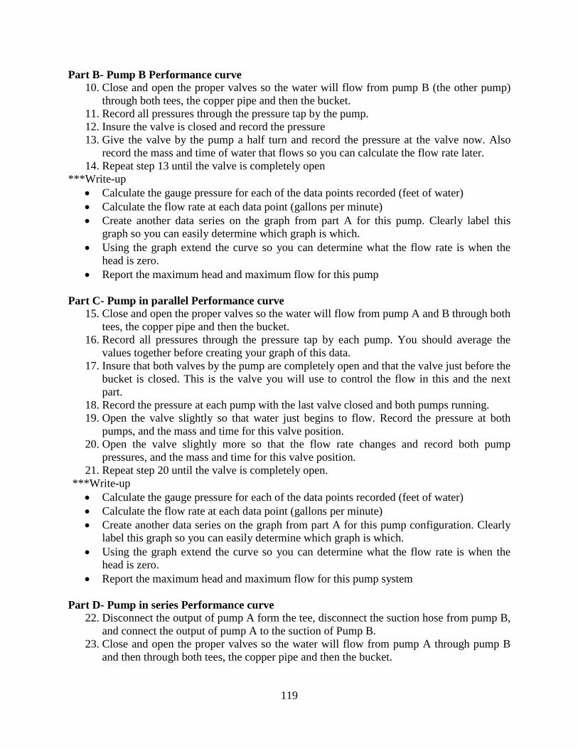
119

Part B- Pump B Performance curve 10. Close and open the proper valves so the water will flow from pump B (the other pump)

through both tees, the copper pipe and then the bucket. 11. Record all pressures through the pressure tap by the pump. 12. Insure the valve is closed and record the pressure 13. Give the valve by the pump a half turn and record the pressure at the valve now. Also

record the mass and time of water that flows so you can calculate the flow rate later. 14. Repeat step 13 until the valve is completely open

***Write-up • Calculate the gauge pressure for each of the data points recorded (feet of water) • Calculate the flow rate at each data point (gallons per minute) • Create another data series on the graph from part A for this pump. Clearly label this

graph so you can easily determine which graph is which. • Using the graph extend the curve so you can determine what the flow rate is when the

head is zero. • Report the maximum head and maximum flow for this pump

Part C- Pump in parallel Performance curve

15. Close and open the proper valves so the water will flow from pump A and B through both tees, the copper pipe and then the bucket.

16. Record all pressures through the pressure tap by each pump. You should average the values together before creating your graph of this data.

17. Insure that both valves by the pump are completely open and that the valve just before the bucket is closed. This is the valve you will use to control the flow in this and the next part.

18. Record the pressure at each pump with the last valve closed and both pumps running. 19. Open the valve slightly so that water just begins to flow. Record the pressure at both

pumps, and the mass and time for this valve position. 20. Open the valve slightly more so that the flow rate changes and record both pump

pressures, and the mass and time for this valve position. 21. Repeat step 20 until the valve is completely open.

***Write-up • Calculate the gauge pressure for each of the data points recorded (feet of water) • Calculate the flow rate at each data point (gallons per minute) • Create another data series on the graph from part A for this pump configuration. Clearly

label this graph so you can easily determine which graph is which. • Using the graph extend the curve so you can determine what the flow rate is when the

head is zero. • Report the maximum head and maximum flow for this pump system

Part D- Pump in series Performance curve

22. Disconnect the output of pump A form the tee, disconnect the suction hose from pump B, and connect the output of pump A to the suction of Pump B.

23. Close and open the proper valves so the water will flow from pump A through pump B and then through both tees, the copper pipe and then the bucket.

120

24. Record all pressures through the pressure tap by each pump. You will use the pressure tap by the last pump to graph your data.

25. Insure that both valves by the pump are completely open and that the valve just before the bucket is closed. This is the valve you will use to control the flow in this and the next part.

26. Record the pressure at each pump with the last valve closed and both pumps running. 27. Open the valve slightly so that water just begins to flow. Record the pressure at both

pumps, and the mass and time for this valve position. 28. Open the valve slightly more so that the flow rate changes and record both pump

pressures, and the mass and time for this valve position. 29. Repeat step 28 until the valve is completely open.

***Write-up • Calculate the gauge pressure for each of the data points recorded (feet of water) • Calculate the flow rate at each data point (gallons per minute) • Create another data series on the graph from part A for this pump configuration. Clearly

label this graph so you can easily determine which graph is which. • Using the graph extend the curve so you can determine what the flow rate is when the

head is zero. • Report the maximum head and maximum flow for this pump system

Overall write-up:

• Tabulate the data for maximum head and flow rate in a table for all four experiments. • Using the tabulated data and the graph that you have created what conclusions can you

draw regarding pumps in parallel and pumps in series? (Your final conclusions should be summarized in a sentence or two but it will take more writing to justify your conclusions.

• Looking at the attached graphs, how does our data compare with the companies' results? Please describe any sources of error and ideas for how to reduce the errors.

121

Pump A- Little Giant 4 MD

Pump B- March AC-3C-MD

122

CEE 1402 Fluid Mechanics Laboratory Lab 8- Open Channel Flow with Spillway and Hydraulic Jump Objectives: Further understanding of flow over a spillway can be learned from this experiment and analysis. The water depth immediately downstream of the spillway is indicated by Y1 and that downstream from the hydraulic jump is Y2. One can apply the continuity equation and the Bernoulli equation to calculate the velocities, V1 and V2, at the two sections. Y1

2-Y22=q2/g(1/Y2-1/Y1) (1)

Where q is the flow per unit width of channel. This value can be used to calculate the velocity, V1, just after the spillway and the velocity, V2, after the hydraulic jump:

V

qY (2)

in which Y is the depth of water where the Froude Number is:

Fr

V

g Y⋅ (3)

The water depth at the crest of the spillway is indicated by Yc, known as the critical depth. The velocity head at this section follows the condition: Fr = Fc = 1 = Vc / (gYc)1/2 or Vc = (gYc)1/2 (4)

By transforming this equation, it can also be used to obtain q, the flow rate per unit width: q = Q/L = VcYc = (gYc3)1/2 (5) The flow over a sharp crested weir can be found using the equation below: Q=Cd*(2/3)*(2*g)^.5 *b*Y^(3/2) (6) Cd= .61 + .08*(Y/h) (7) b= channel width, h= height of the weir, Y= height of water above the weir, sufficiently far from the nappe

123

Procedure and Analysis:

Part A ( use centimeters and newtons)

Completely close the aluminum gate at the end of the flume and allow the water to develop a steady state of flow over top of the aluminum gate. The duty cycle for the pump will be initially set at 25 Hz. Record the necessary information from below and adjust the pump speed to 27.5 Hz and 30 Hz to complete this part of the experiment. Make a sketch and label your measurement points. You will use equation (6) to find the flow of water, therefore determine and measure the required information. We will use the steel bucket to “catch” 5 seconds of water. You will use this to verify the results of the experiment and equation. You will also want to record the height of the water just as it flows over the top of the sharp crested weir, we will use this value in part B.

Part B ( use centimeters and newtons)

The duty cycle for the pump will be initially set at 25 Hz. Record the necessary information from below and adjust the pump speed to 27.5 Hz and 30 Hz to complete this part of the experiment. Completely open the gate at the end of the flume to remove any hydraulic jump. Then adjust the height of the gate to create a hydraulic jump that is several feet away from the gate. Make a sketch and label your measurement points. Establish a flow with a hydraulic jump in the section of the flume after the spillway and measure the water depths Y1 and Y2. The depth of flow will fluctuate approximately 1.5 cm. Record the depth values as +/- 1 cm. Also record the height of the water at the leading edge of the Olgee Spillway and the depth of the water approximately 12 cm upstream of the spillway.

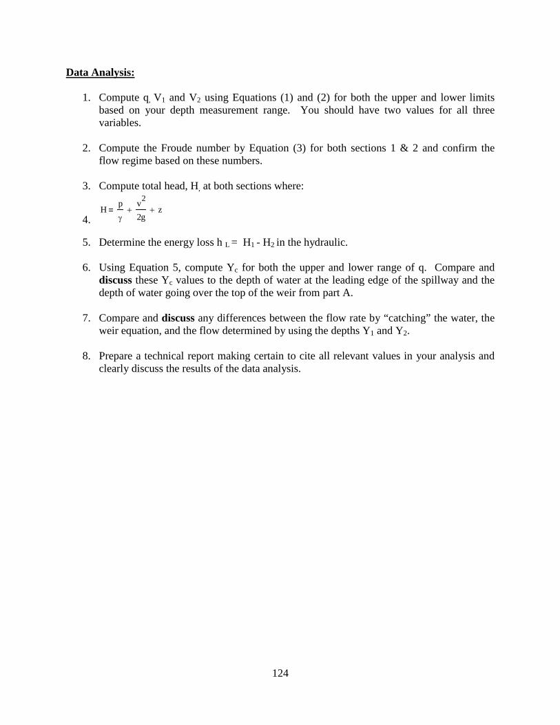
124

Data Analysis:

1. Compute q, V1 and V2 using Equations (1) and (2) for both the upper and lower limits based on your depth measurement range. You should have two values for all three variables.

2. Compute the Froude number by Equation (3) for both sections 1 & 2 and confirm the

flow regime based on these numbers.

3. Compute total head, H, at both sections where:

4. H

pγ

v2

2g+ z+

5. Determine the energy loss h L = H1 - H2 in the hydraulic.

6. Using Equation 5, compute Yc for both the upper and lower range of q. Compare and discuss these Yc values to the depth of water at the leading edge of the spillway and the depth of water going over the top of the weir from part A.

7. Compare and discuss any differences between the flow rate by “catching” the water, the

weir equation, and the flow determined by using the depths Y1 and Y2.

8. Prepare a technical report making certain to cite all relevant values in your analysis and clearly discuss the results of the data analysis.

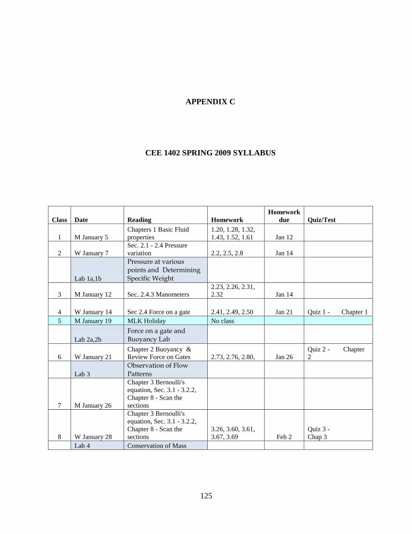
125

APPENDIX C

CEE 1402 SPRING 2009 SYLLABUS

Class Date Reading Homework

Homework due Quiz/Test

1 M January 5 Chapters 1 Basic Fluid properties

1.20, 1.28, 1.32, 1.43, 1.52, 1.61 Jan 12

2 W January 7 Sec. 2.1 - 2.4 Pressure variation 2.2, 2.5, 2.8 Jan 14

Lab 1a,1b

Pressure at various points and Determining Specific Weight

3 M January 12 Sec. 2.4.3 Manometers 2.23, 2.26, 2.31, 2.32 Jan 14

4 W January 14 Sec 2.4 Force on a gate 2.41, 2.49, 2.50 Jan 21 Quiz 1 - Chapter 1 5 M January 19 MLK Holiday No class

Lab 2a,2b Force on a gate and Buoyancy Lab

6 W January 21 Chapter 2 Buoyancy & Review Force on Gates 2.73, 2.76, 2.80, Jan 26

Quiz 2 - Chapter 2

Lab 3 Observation of Flow Patterns

7 M January 26

Chapter 3 Bernoulli's equation, Sec. 3.1 - 3.2.2, Chapter 8 - Scan the sections

8 W January 28

Chapter 3 Bernoulli's equation, Sec. 3.1 - 3.2.2, Chapter 8 - Scan the sections

3.26, 3.60, 3.61, 3.67, 3.69 Feb 2

Quiz 3 - Chap 3

Lab 4 Conservation of Mass

126

Class Date Reading Homework Homework

due Quiz/Test

9 M February 2 Sec. 4.1 - 4.4 Conservation of Mass

4.19, 4.21, 4.22, 4.24, 4.47 Feb 4

10 W February 4 Review for test and Conservation of Energy 4.66, 4.67, 4.69 Feb 11

Lab Review for Test 11 M February 9 Test 1 Test 1 Chap 1 - 4.4

12 W February 11 Sec. 4.5 Conservation of Energy

4.78, 4.83, 4.91, 4.93 Feb 16

Lab 5a,5b Conservation of Energy and Momentum

13 M February 16 Sec. 4.6 - 4.8 Conservation of Energy

4.55, 4.56, 4.86, 4.94 Feb 18

Quiz 4 Chap 4

14 W February 18 Sec. 4.6 - 4.8 Conservation of Momentum

4.111, 4.114, 4.115, 4.117 Feb 23

Quiz 5 Chap 4

Lab Review for test

15 M February 23 Sec. 4.6 - 4.8 Conservation of Momentum

4.112, 4.113,4.122, 4.137 Feb 25

16 W February 25 Review for test Last year’s test 2 Quiz 6 Chap 4

Lab No lab

17 M March 2 Test 2 Test 2 Chap 4

18 W March 4 Sec. 7.1 - 7.3, 7.6 Internal Flow

7.1, 7.4, 7.6, 7.9, 7.20, 7.32, 7.82, 7.85, 7.102 March 16

19 M March 9 Spring Break No Class 20 W March 11 Spring Break No Class

Lab 6 Head Loss in Piping Systems

21 M March 16 Sec. 7.7 Pumps

7.115, 7.118, 7.121, 7.129, 7.130 March 18

22 W March 18 Sec. 7.7

7.87, 7.104, 7.131, 7.134, 7.135 March 23

Quiz 7 Chap 7

Lab 7 Pumps in Parallel and Series

23 M March 23 Review Chapter 7 7.140, 7.141, 7.142 March 25

24 W March 25 Sec. 10.1 - 10.6 Open Channel

10.4, 10.6, 10.8 Last year’s test 3 March 30

Quiz 8 Chap 7

Lab Review for test 25 M March 30 Review for test

26 W. April 1 Test 3 Test 3 Chap 4, 7, 10

Lab 8 Open Channel Flow

127

Class Date Reading Homework Homework

due Quiz/Test

27 M. April 6 Sec. 12.1 - 12.4 Turbomachinery

10.13, 10.40, 12.2, 12.6, 12.8, 12.12, 12.15 April 8

26 W April 8 Sec. 12.5 - 12.6 Turbomachinery

12.28, 12.30, 12.38 April 13

Quiz 9 Chapter 10

Lab Review for final

27 M April 13 Chapter 13 Measurements in Fluids 13.7, 13.8 April 15

Quiz 10 - Sec. 12.1 - 12.4

30 W April 15 Review

31 M April 20 Final Exam classroom 10 am. -

noon Final Exam Chap 1 - 10, 13,14

128

APPENDIX D

FUNDAMENTALS OF FLUIDS SELF-ASSESSMENT SURVEY

The survey is on the following page to preserve the formatting and reproducibility of the

document.

129

130

APPENDIX E

SEMESTER EVALUATION FORM

The evaluation survey is on the following page to preserve the formatting and reproducibility of

the document.

131

132

BIBLIOGRAPHY

Anderson, J.R. (1999). Learning and Memory, An Integrated Approach. NY: Wiley.

Black, R. M. (1996). Design & Manufacture- An Integrated Approach. London: Macmillan Press LTD.

Budny, D.D., W. LeBold, and S. Ward (1992). “Mathematical Self-Concept Development.” 1992 ASEE Annual Conference Proceedings, June 21-25, 1992, Toledo, OH.

Borrego, M. (2007). ”Development of Engineering Education as a rigorous discipline: A Study of the Publication Patterns of Four Coalitions.” Journal of Engineering Education 96(1):5-18.

Chehab, A., A. El-Hajj, M. Al-Husseini, and H. Artail (2004).” Spreadsheet Applications in Electrical Engineering: A Review.” International Journal of Engineering Education 20(6):902-908.

Clarke, G. M. and D. Cooke (1992). A Basic Course in Statistics 3rd Edition. London: Edward Arnold- A Division of Hodder & Stoughton.

Curriculum (2009). In Merriam-Webster Online Dictionary. Retrieved March 9, 2009, from http://www.merriam-webster.com/dictionary/curriculum.

Dym, C.L. and J.S. Rossmann (2004). “On Designing engineering Education: Lessons Learned

at Mudd Design Workshop IV.” International Journal of Engineering Education 20(3):470-473.

EAC- Engineering Accreditation Commission (2008). "Criteria for Accrediting Engineering Programs."http://www.abet.org/Linked%20Documents-UPDATE/Criteria%20and%20PP/E001%2009-10%20EAC%20Criteria%2012-01-08.pdf.

Felder, R.M. and R. Brent (2003). “Designing and Teaching Courses to Satisfy the ABET Engineering Criteria.” Journal of Engineering Education 92(1):7-25.

Feinstein, A.R. (2001). Principles in Medical Statistics. New York: Chapman and Hall.

133

Fraser, D. M., R. Pillay, L. Tjatindi, and J.M. Case (2007). “Enhancing the Learning of Fluid Mechanics Using Computer Simulations.” Journal of Engineering Education 96(4):381-387.

Hesketh, R.P. and C.S. Slater (2000). “Innovative and Economical Bench-Scale Process Engineering Experiments.” International Journal of Engineering Education 16(4):327-334.

Hestenes, D., M. Wells, and G. Swackhamer (1992). “Force Concept Inventory.” The Physics Teacher 30(3)141-151.

Higley, K.A. and C.M. Marianno (2001). “Making Engineering Education Fun.” Journal of Engineering Education 90(1):105-107.

Hise, R.T., L. O’Neal, J.C. McNeal, and A. Parasuraman (1989). “The Effect of Product Design Activities on Commercial Success Levels of New Industrial Products.” Journal of Prodcut Innovation Management 6(1):43-50.

Kresta, M.S. (1998). “Hands-on Demonstrations: An Alternative to Full Scale Lab Experiments.” Journal of Engineering Education 87:7-9.

Kumar, R. and A. O. Al-Sahantaf (1997). “Spreadsheet Analysis of Fluid Mechanics Problems.” FIE Conference- Teaching & Learning in an Era of Change Proceedings 3:1334-1337.

Kreyszig, E. (1973). Introductory Mathematical Statistics. New York: John Wiley & Sons, Inc.

Lamancusa, J. S. (2006). “Design as the Bridge Between Theory and Practice.” International Journal of Engineering Education 22(3):652-658.

LeBold, W.K., W. Zink, S.E. Scott, and G. Salvendy (1987). “Programming Perceptions and Computer Literacy of Students Enrolled in Computer-Related Curricula.” IEEE Transaction in Education 30(4):201-211.

LeBold, W.K., R. Montgomery, D. Budny, G. Bjedov, and S. Ward (1998). “Assessing Computer Literacy and Achievement Using Self-Concepts.” Proceeding of the 28th Annual Frontiers in Education 1:1-7.

Martin, J., J. Mitchell, and T. Newell (2003). “Development of a Concept Inventory for Fluid Mechanics.” 33rd ASEE/IEEE Frontiers in Education Conference T3D:23-28.

Martin, J., J. Mitchell, and T. Newell (2004). “Work in Progress: Analysis of Reliability of the Fluid Mechanics Concept Inventory.” 34th ASEE/IEEE Frontiers in Education Conference F1F:3-4.

Maxiner, M.R. (1999). “The Use of MathCad in Teaching Ideal Fluid Flow with Complex Variables.” International Journal of Engineering Education 15(6):456-468.

134

Merrill, M.D. (2001). “Components of Instruction Toward a Theoretical Tool for Instructional Design.” Instructional Science 29:291-310.

Merril, M. D. (2002). “First Principles of Instruction.” Educational Technology Research & Development 50(3):43-59.

Nasarazadani, S. (2007). “Design and Construction of a Heat Exchanger Analyzer for an Undergraduate Thermal-Fluids Laboratory.” International Journal of Engineering Education 23(3):618-628.

Olinger, D. J. and J. C. Hermanson (2002). “Integrated Thermal-Fluid Experiments in WPI’s Discovery Classroom.” Journal of Engineering Education 91(2):239.244.

Otto, K. N. (2001). Product Design: Techniques in Reverse Engineering and New Product Development. Upper Saddle River, NJ: Prentice Hall.

Pavelich, M.J. and W. S. Moore (1996). “Measuring the Effect of Experiential Education Using the Perry Model.” Journal of Engineering Education 85(4):287-292.

Pomales-Garcia, C. and Y. Liu (2007). “Excellence in Engineering Education: Views of Undergraduate Engineering Students.” Journal of Engineering Education 96(3):253-262.

Prince, M. (2004). “Does Active Learning Work? A Review of the Research.” Journal of Engineering Education 93:223-231.

Reddish, E.F., J. M. Saul, and R. N. Steinberg (1998). “Student Expectations in Introductory Physics.” American Journal of Physics 66(3):212-224.

Reiser, R.A. (2001). “A History of Instructional Design and Technology: Part II: A History of Instructional Design.” Educational Technology Research & Development 49(2):57-67.

Rowland, G. (1993). “Designing and Instructional Design.” Educational Technology Research & Development 41(1):79-91.

Ryan, B., B. Joiner, and J. Cryer. (2005). Minitab Handbook- Updated for Release 14. Belmont, CA: Brooks/Cole Thompson Learning.

Sarin, S. and D. Headley (2002). “Validity of Student Self-Assessments.” Proceedings of the 2002 ASEE Annual Conference, Session 3530.

Schunn, D. (2008). “Engineering Educational Design.” Educational Designer, 1(1). Retrieved February 28, 2009, from http://www.educationaldesigner.org/ed/volume1/issue1/article2 .

Schwartz, T.L. and Dunkin B.M. (2000). “Facilitating Interdisciplinary Hands-on Learning using LabVIEW.” International Journal of Engineering Education 16(3):218-227.

Smith, S.M., T.B. Ward, and J.S. Schumacher (1993). “Constraining Effects of Examples in a Creative Generations Task.” Memory and Cognition 21(6):837-845.

135

Tripp, S. D. and B. Bichelmeyer (1990). Rapid Prototyping: An Alternative Instructional Design Strategy. Educational Technology Research & Development 38(1):31-44.

Welch, R. W. and J. L. Klosky (2007). An Online Database and User Community for Physical Models in the Engineering Classroom.” Advances in Engineering Education 1(1):1-25.

Wicker, R.B. and R. Quintana (2000). “An Innovation-Based Fluid Mechanics design and Fabrication Laboratory.” Journal of Engineering Education 89(3):361-367.

Zoller, U. and D. Ben-Chaim (1998). “Student Self-Assessment in HOCS Science Examinations: Is There a Problem?” Journal of Science Education and Technology 7(2):135-147.