PRODUCT INNOVATION IN DURABLEGOODS MONOPOLY WITH PARTIAL

PHYSICAL OBSOLESCENCE

A Master’s Thesis

byAYSUN ATIL

Department ofEconomics

Bilkent UniversityAnkara

September 2007

To Asil Atıl

PRODUCT INNOVATION IN DURABLEGOODS MONOPOLY WITH PARTIAL

PHYSICAL OBSOLESCENCE

The Institute of Economics and Social Sciencesof

Bilkent University

by

AYSUN ATIL

In Partial Fulfillment of the Requirements For the Degreeof

MASTER OF ARTS

in

THE DEPARTMENT OFECONOMICS

BILKENT UNIVERSITYANKARA

September 2007

I certify that I have read this thesis and have found that it is fully adequate, in

scope and in quality, as a thesis for the degree of Master of Arts in Economics.

Assist. Prof. Dr. Kevin Hasker

Supervisor

I certify that I have read this thesis and have found that it is fully adequate, in

scope and in quality, as a thesis for the degree of Master of Arts in Economics.

Assist. Prof. Dr. Cagla Okten

Examining Committee Member

I certify that I have read this thesis and have found that it is fully adequate, in

scope and in quality, as a thesis for the degree of Master of Arts in Economics.

Assoc. Prof. Dr. Suheyla Ozyıldırım

Examining Committee Member

Approval of the Institute of Economics and Social Sciences

Prof. Dr. Erdal Erel

Director

ABSTRACT

PRODUCT INNOVATION IN DURABLE GOODS

MONOPOLY WITH PARTIAL PHYSICAL

OBSOLESCENCE

Atıl, Aysun

M.A., Department of Economics

Supervisors: Assist. Prof. Dr. Kevin Hasker

September 2007

In the literature on planned obsolescence, it has always been assumed that

the durable goods monopolist is able to limit the durability of the whole of

the product. However, usually it is a component of the product rather than

the whole unit that becomes physically obsolete. In this paper, we analyze

R&D incentives of a durable goods monopolist when he is able to engage

in partial physical obsolescence. We showed that under these circumstances

competition in component goods market causes inefficient R&D decisions in

the primary market.

Keywords: Planned Obsolescence, Innovation, Component Goods.

iii

OZET

KISMI FIZIKSEL ASINMALI DAYANIKLI MALLAR

TEKELINDE URUN YENILIGI

Atıl, Aysun

Yuksek Lisans, Ekonomi Bolumu

Tez Yoneticisi: Yrd. Doc. Dr. Kevin Hasker

Eylul 2007

Planlanmıs amortisman literaturunde, her zaman varsayılmıstır ki dayanıklı

mallar ureten tekelci urunun tamamının dayanıklılıgını sınırlandırabilir. An-

cak urunun tamamından ziyade genelde urunun bir parcası fiziksel olarak kul-

lanılmaz hale gelir. Bu tezde, kısmi fiziksel asınma uygulayabilen dayanıklı

mallar ureten tekelcinin AR-GE egilimlerini inceledik. Bu kosullar altında,

parca mallar piyasasındaki rekabetin orijinal urun piyasasında verimsiz AR-

GE kararlarına neden oldugunu gosterdik.

Anahtar Kelimeler: Planlanmıs amortisman, Yenilik, Parca mallar.

iv

ACKNOWLEDGEMENTS

I would like to thank to my supervisor Kevin Hasker for his continual

guidance for this thesis.

I am indebted to Cagla Okten for her guidance through the development

of this thesis and thank to for her invaluable comments.

I would like to thank to H. Cagrı Saglam who spared his time to teach

and encourage me.

I am grateful to Tarık Kara and Ferhad Huseyinov for their invaluable

suggestions.

Finally I owe special thanks to Umran Atıl, Saniye Atıl, Aytul Kaygısız,

Efsun Kızmaz and Oguz Yılmaz for their endless support and patience.

v

TABLE OF CONTENTS

ABSTRACT . . . . . . . . . . . . . . . . . . . . . . . . . . . . . iii

OZET . . . . . . . . . . . . . . . . . . . . . . . . . . . . . . . . . iv

ACKNOWLEDGEMENTS . . . . . . . . . . . . . . . . . . . . . v

TABLE OF CONTENTS . . . . . . . . . . . . . . . . . . . . . . vi

CHAPTER 1: INTRODUCTION . . . . . . . . . . . . . . . . . 1

CHAPTER 2: LITERATURE REVIEW . . . . . . . . . . . . . 5

CHAPTER 3: THE MODEL . . . . . . . . . . . . . . . . . . . 14

CHAPTER 4: THE SOCIAL OPTIMUM . . . . . . . . . . . . 17

CHAPTER 5: THE EQUILIBRIUM WHEN THE

MONOPOLIST CONTROLS THE COMPONENT

MARKET . . . . . . . . . . . . . . . . . . . . . . . . . . . . . 24

CHAPTER 6: THE EQUILIBRIUM WHEN THE

COMPONENT MARKET IS PERFECTLY

COMPETITIVE . . . . . . . . . . . . . . . . . . . . . . . . . 34

CHAPTER 7: THE EQUILIBRIUM WHEN THE

COMPONENT MARKET IS IMPERFECTLY

COMPETITIVE . . . . . . . . . . . . . . . . . . . . . . . . . 42

CHAPTER 8: CONCLUSION . . . . . . . . . . . . . . . . . . . 53

vi

BIBLIOGRAPHY . . . . . . . . . . . . . . . . . . . . . . . . . . 55

APPENDIX . . . . . . . . . . . . . . . . . . . . . . . . . . . . . . 57

vii

CHAPTER 1

INTRODUCTION

Durability choice and the related issue of planned obsolescence are main

concerns of the analyses in durable goods theory. Planned obsolescence is

defined as the production of goods with uneconomically short useful lives

(Bulow, 1986). In the literature on planned obsolescence by a durable-good

monopoly, it has always been assumed that the monopolist is able to limit

the durability of the whole of the product. However, for the most durable

goods such as personal computers, automobiles, cellphones, stereo systems,

it is not the whole unit that becomes completely obsolete, but a component

of a durable good. For example, it is the battery not the cellphone, the toner

fluid not the photocopier, the car parts not the car itself that die first. This

requires analyzing the incentives of a durable good monopolist with regard

to the component durability. Recently, components and component related

service markets gained the attention within the context of pricing decisions

without any possible links to R&D incentives.

In this paper, we study the R&D incentives of a durable good monopolist

when he is able to engage in partial physical obsolescence, which refers to the

obsolescence of components. We use the model in Fishman and Rob (2000)

and adopt it to our setting of planned partial physical obsolescence.

Fishman and Rob (2000) investigate a durable good monopolist’s R&D

1

incentive in a model with identical consumers under the assumption that in-

novations are recurrent and knowledge builds up cumulatively. They find

that the monopolist innovates less frequently and invests less than the ef-

ficient level. The reasoning is as follows: When a new model appears, old

models in consumers’ possession are still physically functional. Consumers

are willingly to pay for the incremental flow of services provided by the new

model —until it’s replaced by an upgraded model. However, the introduction

of a new model increments consumers’ utility in perpetuity since the new

model forms the technological base for the subsequent models. This implies

that the monopolist receives less than the social value of an innovation. In

order to compensate this loss, the monopolist waits longer between prod-

uct innovations, thereby lengthening the period which consumers pay for the

services provided by the new model. Fishman and Rob (2000) also suggest

that if the monopolist is able to design each model to last until the new one

is introduce-in other words engage in planned obsolescence, the monopolist

gets the social value of each model and is induced to innovate at the socially

optimal pace.

However, as we state above usually it is a component that becomes phys-

ically obsolete. The competitive environment that these components are pro-

duced become important for a durable good monopolist’s R&D incentives.

With regard to this, we extend Fishman and Rob’s analysis.

We incorporate the component durability by allowing the monopolist to

engage in partial physical obsolescence. The monopolist introduces the new

model as the component of the previous model obsoletes. In that case, the

monopolist is able to charge consumers both for the incremental utility and

the replacement cost of the component. For example, consider a Xerox printer.

The price for one of the models of a Xerox printer is $189, while its component

is sold at a price of $100.55. Moreover, repair costs related to Xerox machines

are quoted at least $50 and there is also an extra cost depending on the

2

damage. This implies replacing the component costs as much as buying a

new product. Under these circumstances, we find that if the monopolist

controls the component market, he innovates at the socially optimal pace.

However, if the component market is perfectly competitive, like in Fishman

and Rob (2000) the monopolist innovates less frequently and invests less than

the socially optimal level.

The main concern of this paper is to analyze R&D incentives in the pres-

ence of partial physical obsolescence; nevertheless the insights of this study

also contribute to the aftermarket literature. Aftermarkets are markets for

spare parts, repairs, services and upgrades, etc. The aftermarket good or

service is used together with the original equipment, but is sold after the

purchase of the equipment (Chen, 1998). In this context, components market

can be considered as an aftermarket.

Recently, a number of important court cases in USA, Canada and Europe

has indicated the importance of the aftermarkets. For example, in the Ko-

dak and Xerox cases, the original equipment manufactures were sued for the

attempts to monopolize their aftermarket. One of the questions arising out

of these court cases is that “Does the monopolization of the aftermarket by

the original equipment manufacturers cause an efficiency loss?”.

Borenstein et. al. (2000), point out that many independent service

providers for high technology products have sued equipment manufacturers

for allegedly excluding them from providing maintenance services. They show

that price in the services and parts market (aftermarket) will exceed marginal

cost despite the competition in the equipment market. Chen and Ross (1998)

observe that both in USA and Europe a number of anti-trust cases have

involved allegations that manufacturers of durable goods have refused to sup-

ply parts to independent service organizations, apparently to monopolize the

market for repairs of their products. They study such refusals in a competitive

market and its connected aftermarket and find that refusals help to support

3

higher prices for high value users but at the same time permit the recovery

of higher costs incurred during an initial warranty period. Since full prices

reflect full marginal costs at equilibrium, the refusals permit the attainment

of a first-best outcome. Accordingly, an attempt by anti-trust authorities to

force supply would be welfare reducing. Similarly in terms of R&D decisions,

we find that if the component good market becomes more competitive, the

R&D investments depart more from its socially optimal level. Hence, the

monopolization of the components market is welfare inducing.

The distinct feature of our model is the presence of partial physical

obsolescence- namely a component becomes obsolete. We analyze the ef-

fects of the market structure in the components market on R&D decisions of

a durable good monopolist and find that if the monopolist engages in partial

physical obsolescence, then the competition in the component market causes

innovations to depart from socially optimal level. When there is perfect com-

petition in the component market, our analysis of monopoly equilibrium is

same as Fishman&Rob’s (2000) analysis of monopoly equilibrium without

obsolescence. We should note that although much of our discussion concerns

durable goods monopolists, this does not mean that the insights from our

analysis only apply to such settings. Even though most durable goods pro-

ducers are not monopolists, most do have market power so that monopoly

analysis should provide useful insights.

In the next chapter, we present relevant literature in planned obsolescence.

In Chapter 3, we set up the basic framework of our model and in Chapter 4,

we analyze the social optimum. Chapter 5 contains the analysis of monopoly

equilibrium when the monopolist controls the component market. Chapter

6 and 7 contain respectively analyses of monopoly equilibrium, first with

perfect competitive component market and second with imperfect competitive

component market. In Chapter 8, we present our results.

4

CHAPTER 2

LITERATURE REVIEW

Recently two issues have generated controversy in durable goods litera-

ture: (i) Do firms have an incentive to reduce durability below socially opti-

mal level? (ii) To what extent do firms have an incentive to introduce new

products that make old units obsolete? The main concern of these issues is

actually to explore whether firms engage in ”planned obsolescence” or not.

Analyses related to the planned obsolescence in durable goods theory can

be grouped in two categories. First group, which includes Coase (1972),

Bulow (1986) and Swan (1972) accept the definition that planned obsolescence

is the production of goods with uneconomically short useful lives. Second

group leading by Waldman (1993; 1996), Choi (1994) and Kumar (2002)

suggest that planned obsolescence is about how often a firm will introduce

new products that make old units obsolete. Therefore, the first approach to

planned obsolescence can be considered in terms of durability choice whereas

the second approach to planned obsolescence can be considered in terms of

R&Ddecisions. Within this context, several authors analyze the incentives of

a durable goods monopolist who sells its products.

Coase (1972) considers the dynamic pricing problem of a monopoly selling

a durable good to consumers with different valuations. He suggests that

durable goods monopolist faces a time inconsistency problem. The problem

5

arises since durable goods sold in the future affect the value of units sold

today. In the absence of ability to commit to future prices, the monopolist

does not internalize this effect. Coase argues that under these circumstances

the price must eventually fall as the market clears high-valuation consumers.

In Coase’s analysis, planned obsolescence restores the monopoly’s ability to

charge monopoly prices.

Following Coase’s conjecture (Coase, 1972), Bulow (1982; 1986), considers

a durable good monopolist who sells output in each of two periods. If the

monopolist is unable to commit to future production levels, in the second

period he will choose the production level which maximizes its second period

profits. However, additional units in the second period reduces the second

period value of the units previously sold. Rational consumers who anticipate

this reduction are not willing to pay higher prices in the first period and as a

result overall monopoly profits fall. Bulow argues that by reducing durability

of its output, the durable goods monopolist can solve its time inconsistency

problem.

Swan (1972) handles the issue of planned obsolescence in terms of durabil-

ity choice incorporating secondhand markets to the analysis. In the context

of automobile market, he examines the optimal durability choice of a durable

goods monopolist when new and used cars are perfect substitutes. Given a

flexible production policy, the monopolist would like the minimize the cost of

any given service flow from a stock of durable goods. Consumers are willing

to pay higher prices for new goods if they also receive higher prices for their

trade-ins. Swan argues that given the inelastic demand for used cars limiting

durabilty enables the monopolist to reduce the flow of services provided by

used cars, thereby increasing used car prices. However, a monopolist cen re-

strict the supply of future used cars by varying the price of new goods rather

than varying the durability level. Swan shows that for the durable goods

monopolist there is no distortion in terms of durability.

6

Related to Swan’s analysis (Swan, 1972), Rust (1986) also considers the

optimal durability choice of a durable goods monopolist when there is a sec-

ondary market for used durable goods. He suggests that secondary market

provides close substitutes for new durable goods limiting profits of the monop-

olist in the primary market. By limiting product durability, the monopolist

ensures that used goods are worse substitutes for new goods. Contrary to

Swan, Rust also argues that it is not the existence of secondary markets,

but the endogenous scrappage of durables which provides consumers with

a substitution possibility that constraints monopoly profits. He considers a

Stackelberg game between the monopolist and consumers and shows that for

some specific values of parameters the selling monopolist prefers to kill off

the secondary market by reducing durability.

Samuelson and Bond (1987) analyze the effects of durability on the incen-

tives to innovate. They argue that since future price of a durable good affects

the current demand for that good, durability creates incentives to innovate.

They consider a monopoly that sells a durable good in two periods, with the

cost of production in each period depending on investments in R&D. Since

some costs of increasing output is not internal to the firm, the monopolist

can increase its output in order to exploit the residual demand he faces in the

second period. Expanding output increases the marginal profitabilty of inno-

vation. However, the standard incentive of the monopolist to reduce output

below its socially optimal level has a diverse effect on innovation. Therefore,

depending on which one of these conflicting effects dominates, the selling

monopolist invests less or more on innovation than is socially optimal.

The common approach accepted in planned obsolescence (in terms of dura-

bility choice) literature is that the monopolist is able to limit the durability of

whole of the product. Within this context, the economic motives for and wel-

fare consequences of limiting product durability in durable goods monopoly

are analyzed. However, usually a component of a product rather than the

7

whole good becomes obsolete. In this paper, different than the previous lit-

erature, we handle the issue of planned obsolescence in terms of component

durability, which we refer as ”partial physical obsolescence”.

Waldman (1993; 1996), Choi (1994), and Kumar (2002) have also consid-

ered that the introduction of a new product can lower the value of used units.

Waldman (1996) demonstrates that a similar result to that in Coase (1972)

and Bulow (1986) holds within the context of the monopolist’s R&D expendi-

tures. Since the monopolist does not internalize in the second period how its

behavior affects the value of units sold previously, the monopolist’s incentive

to invest in R&D that makes past production ”technologically obsolete” is

too high. Hence in that paper the term planned obsolescence is used to mean

that the monopolist has an incentive to engage in R&D decisions and new

products introductions and thereby make the past production technologically

obsolete. Waldman finds that although time inconsistency causes overinvest-

ment in R&D from the standpoint of the monopolist’s own profitability, from

the standpoint of social welfare the time inconsistency problem is in fact ben-

eficial. He finds that in the case where the monopolist can commit to a future

value for R&D, the firm is unable to capture all the societal benefits from the

improved quality of its output. As a result the private incentive to invest in

R&D is less than the incentive that is social welfare maximizing.

Like Waldman (1996), Choi (1994) examines the economic incentives for

inducing incompatibilities between generations of products and explores the

welfare consequences of the product differentiations. He considers a durable

goods monopolist who offers products in each of two periods and determines

to introduce a compatible or an incompatible product in the second period.

He argues that if the monopolist is able to price discriminate between old

and new customers, the monopolist prefers to sell an incompatible product to

both type of consumers whereas social efficieny requires to sell a compatible

product only to newcomers. If the monopolist is not able to price discriminate,

8

the society suffers an extreme underconsumption in the first period. In that

case, the monopolist does not offer any product in the first period and social

ineffienciency arises due to no product availability.

Kumar (2002) analyzes the effects of resale trading on the price and qual-

ity decisions of a durable goods monopolist. He considers a durable goods

monopolist who varies price and quality of an infinitely durable product over

time in a market of heterogenous, but rational consumers. He suggests that

time inconsistency problem arises due to intertemporal quality discrimination.

The reason is that quality upgrades may induce high-valuation consumers to

delay purchase, which leads a constraint on monopoly prices. However, by re-

sale trading the monopolist can price discriminate between high-valuation and

low-valuation consumers, thereby overcomes its time inconsistency problem.

Kumar observes that the monopolist’s optimal price and quality offers in new

goods market may have complex dynamic patterns. He shows that because

of future resale trading, the monopolist may introduce a product of ineffi-

cient quality. However, initial quality distortions are followed by steady-state

quality allocations that are always efficient for high-valuation consumers.

Both Waldman (1996) and Choi (1994) have considered planned obsoles-

cence as how often a firm will introduce a new product and how compatible

the new product will be with older products. In both analyses, costs of inno-

vation incurred by firms are ignored. We incorporate investment expenditures

on R&D into the analysis.

Fishman and Rob ’s study (2000) explained in Chapter 1 is the bench-

mark analysis we adopt our model. In the setting of Fishman and Rob,

product durability limits market power by increasing the value of the con-

sumers’ outside option and thereby reducing their willingness to pay for new

models. Hence limiting product durability reduces the value of consumers’

outside options. However, we should note that while the ability to precommit

to future sales completely resolves the Coasian monopoly’s problem a similar

9

ability to precommit to future introduction dates does not accomplish the

same purpose in the context of recurring innovations. It is also important to

note that in the Coasian setting (Coase, 1972), market efficiency is improved

as prices fall, but in Fishman and Rob a monopolist that can not charge

for the social value of an innovation innovates less than the socially efficient

amount.

We analyze R&D incentives of a durable goods monopolist when a com-

ponent that is complementary to the original product obsoletes. Therefore,

the structure of the component market becomes crucial in the analysis of in-

novation activity in the primary market in which original goods are sold. If

we consider components market as an aftermarket, the insights of our study

also contribute to the aftermarket literature.

Chen et al. (1998) analyze the court cases such as Kodak, Chrysler and

Xerox in which original equipment manufacturers are accused of refusing sup-

ply parts to independent service organizations. Chen et al. state that these

refusals by original equipment manufacturers involve attempts to monopolize

their aftermarkets. Furthermore, they provide a summary of the economic

theories of aftermarkets which try to explain the motives of aftermarket mo-

nopolization. One of the aftermarket theories cited in Chen et al. (1998) is

”Consumer Surprise Theory”, which suggests that switching costs may pre-

vent a customer from switching to a different brand even if the prices of the

aftermarket products and services raised substantially. In this way, origi-

nal equipment manufacturers earn abnormal profits by their installed base of

customers. However, this theory is criticized since it does not involve ”repu-

tation effects”, which implies higher aftermarket prices induce potential new

consumers to purchase other brands.

Boreinstein et al. (2000) analyze firms’ two goals- exploiting lock-in cus-

tomers by raising aftermarket prices and limiting its aftermarket prices due to

reputation effects, in a differentiated duopoly model. They examine whether

10

competition in durable goods market prevents manufacturers from exercis-

ing market power over aftermarket products and services. They show that

regardless of the structure of the equipment market, the price in the aftermar-

ket exceeds marginal cost of production. In their model, original equipment

manufacturers monopolize their associated aftermarket goods and firms are

not able to commit to future prices. There is a crucial restriction on demand

side that consumers are always prefer using old units by acquiring services to

purchasing new goods. Boreinstein et al. show that if the option to scrap and

buy new good is binding at the margin, the aftermarket price is increasing

in the degree of firm’s market power in the equipment market. This analysis

does not include the connection between intensity of use and switching costs.

Chen and Ross suggest that aftermarket prices can be used to discriminate

between high intensity- high value users and low intensity- low value users.

They state that higher aftermarket prices are needed to recover the costs of

warranty protection. The reason is that more frequent servicing is required

for high intensity consumers in the post warranty period and if the manufac-

turer can not identify higher intensity customes before purchase, it can not

imbed higher expected costs into their original equipment price. In a compet-

itive market and connected aftermarket where firms are able to commit future

prices, by charging a low price for the primary product, providing a warranty

for the first period and then supracompetitive price for repairs in the second

period, each firm is able to set an expected full price for each customer equal

to marginal costs of serving that customer. Hence, forcing original equipment

manufacturers to supply parts to independent service organizations is welfare

reducing. Chen and Ross’s analysis is an example to ”The Price Discrimi-

nation Theory” cited in Chen et. all, which suggests that aftermarket prices

as a metering device to discriminate between high intensity- high value users

and low intensity- low value users.

Marinoso also analyzes endogenous switching costs that reduce competi-

11

tion in aftermarkets. He suggests that in order to monopolize their aftermar-

ket, firms may use technological incompatibility which creates endogenous

switching costs. In a two period duopoly model, firms introduce a system

which consists of various components in the first period whereas in the second

period they introduce both the system and the complement that is broken.

Endogenous switching costs are driven by second period equilibrium prices

of complements and durables. Marinoso states that if firms are able to price

discriminate between old consumers and newcomers, switching costs do not

affect rational consumers’ initial purchasing decisions. Hence, there is no

connection between aftermarket prices and initial equipment sales. In these

circumstances, introduction of compatible technology in the second period de-

pends on the costs incurred by firms to achieve compatibility. Marinoso shows

that with homogeneous products and small costs of reaching compatibility,

endogenous switching costs induce firms to prefer compatible products.

The studies mentioned above and other aftermarket theories generally fo-

cus on the incentives of original equipment manufacturers to raise aftermarket

prices and its welfare consequences. There has been little research concerning

efficiency losses in terms of R&D decisions due to the structure of the com-

ponent market. Within this context, our study presents a different approach

to the aftermarket literature.

Fishman and Rob (2000) is related to the Coase Conjecture (Coase, 1972)

in the sense that planned obsolescence is a business strategy that help a

durable good monopolist to maintain its market power. Coase (1972) con-

sidered the dynamic pricing problem of a monopoly selling a durable good

(of fixed quality) to consumers with different valuations (Bulow, 1982; 1986).

Coase argued that if the monopoly is unable to commit to future prices (or

equivalently, commit not to sell any more units), the price must eventually

fall as the market clears of high valuation buyers in the second period. In

that setting, planned obsolescence restores the monopoly’s ability to charge

12

monopoly prices. In the setting of Fishman and Rob (2000), product dura-

bility limits market power by increasing the value of the consumers’ outside

option and thereby reducing their willingness to pay for new models. Hence

limiting product durability reduces the value of consumers’ outside options.

However, we should note that while the ability to precommit to future sales

completely resolves the Coasian monopoly’s problem a similar ability to pre-

commit to future introduction dates does not accomplish the same purpose

in the context of recurring innovations. It is also important to note that in

the Coasian setting, market efficiency is improved as prices fall, but in Fish-

man and Rob a monopolist that can not charge for the social value of an

innovation innovates less than the socially efficient amount.

Waldman (1993; 1996), Choi (1994), Kumar (2002) have also considered

that the introduction of a new product can lower the value of used units.

Waldman (1996) demonstrates that a similar result to that in Coase (1972)

and Bulow (1972) holds within the context of the monopolist’s R&D expendi-

tures. Since the monopolist does not internalize in the second period how its

behavior affects the value of units sold previously, the monopolist’s incentive

to invest in R&D that makes past production “technologically obsolete” is

too high. Hence in that paper the term planned obsolescence is used to mean

that the monopolist has an incentive to engage in R&D decisions and new

products introductions and thereby make the past production technologically

obsolete. Waldman finds that although time inconsistency causes overinvest-

ment in R&D from the standpoint of the monopolist’s own profitability, from

the standpoint of social welfare the time inconsistency problem is in fact ben-

eficial. He finds that in the case where the monopolist can commit to a future

value for R&D, the firm is unable to capture all the societal benefits from the

improved quality of its output. As a result the private incentive to invest in

R&D is less than the incentive that is social welfare maximizing.

13

CHAPTER 3

THE MODEL

We consider a monopolist that introduces infinitely durable products peri-

odically. Every period starts with an introduction of a new model and at the

beginning of each period, the monopolist decides on its R&D investment. The

quality level of the current product is q ∈R+. As Fishman and Rob (2000)

state, introduction of a new model is preceded by an R&D stage, called a

“gestation period”. The monopolist has to decide the length of the gestation

period, which is denoted by t and the per period R&D expenditures in it,

which is denoted by x. Quality increment between two consecutive products

is determined by g, which is a function of x and t. Then the quality of the

new model is q + g (x, t).

Like in Fishman and Rob (2000), we allow recurrent introductions and

assume that quality improvements are cumulative1. When the monopolist

introduces a new product, it incurs in addition to R&D expenditures a fixed

cost of F , which is a lump-sum payment. F can be considered an implemen-

tation cost, the amount the monopolist must pay for augmenting the present

product. There is a constant marginal cost of production, c. We assume for

simplicity the production cost is invariant to the quality of the product. We

1Fishman and Rob define recurrent introductions such that the introduction of onemodel triggers the development of the next one. They also assume quality improvements arecumulative: If two models are introduced in sequence, and if their R&D inputs are (x1, t1)and (x2, t2) , then the quality of the second-generation model is q + g (x1, t1) + g (x2, t2)and similarly for later generations.

14

impose the following assumption to ensure that innovation is not too costly

relative to the benefit:

Assumption 1 g is strictly concave, bounded, increasing in x and t, twice

continuously differentiable, g (x, 0) = g (0, t) = 0, and there exists an

{xp, tp} so that r (F + c) < δg (xp, tp)− (ertp − 1) xp where δ ∈ (0, 1] .

r denotes the positive discount rate, which is common for consumers and

firms. We have the first five restrictions on g in order to simplify the analysis.

The last restriction guarantees that the monopolist always invests in R&D

and introduces new models (t < ∞, x > 0).

Different than Fishman and Rob (2000), we have the additional assump-

tion for g in order to achieve concavity around the optimal solution, thereby

obtaining differentiability of the objective function.

Assumption 2 For λ ∈ (0, 1] ,

λ2gxxgtt ≥(λgxt − rert

)2It is just a stronger concavity condition than what is stated in Assumption

3.

There is a finitely durable component good that complements the primary

product. The life of the component coincides with the gestation period. As

the new generation of the primary product is introduced, the component

that is complementary to the current product obsoletes. We assume the

component good is produced at a cost of αc, where α ∈ (0, 1) . Thus, the

production cost of the component is just a constant fraction of the marginal

cost of the primary product.

On the demand side, there is a continuum of identical infinitely lived con-

sumers of measure 1. Each consumer may consume at most one durable good.

A representative consumer derives a flow utility of $q from product of quality,

15

q. When the new generation is introduced, consumers must decide whether

to purchase a new model or to replace the component of the current product.

If the component is replaced, then the flow utility is the same as if they had

bought a new good of the same generation. The price of the component,

which is denoted by pc, is crucial for the monopolist’s R&D decisions since pc

affects the opportunity cost of buying a new model. We assume pc depends

on g, q, αc. We have the following restrictions on pc (g, q, αc):

Assumption 3 pc (g, q, αc) is concave, bounded, increasing in q and twice

continuously differentiable. Moreover, pc ∈ {αc, q} .

The first four assumptions are fairly standard. The last assumption en-

sures that the price of the component can not exceed the flow utility of the

primary product that the component is complementary to and also it can not

be below its production cost.

Throughout our analysis the monopolist sells its products rather than rent

them and there is no secondhand market for the primary product.

16

CHAPTER 4

THE SOCIAL OPTIMUM

We first derive the socially optimal outcome for the innovation activity in

order to detect whether the monopolist’ R&D decisions are efficient or not.

Given the initial quality, q0, the social planner chooses R&D expenditures,

{x1, x2, x3, ...} and gestation periods, {t1, t2, t3, ...}. We can denote the cal-

endar dates at which new models are introduced as Ti, where ∀i, T i =i∑

j=1

tj.

The quality of the model introduced at Ti isi∑

j=1

g (xj, tj) and the social plan-

ner delivers benefits from this model over [Ti, Ti+1). Thus, as of date Ti, it

generates a discounted benefit of

(i∑

j=1

g (xj, tj)

)((1−e−rti+1)

r

). Hence, the

sequential problem for the social planner can be written as follows:

(SP ) sup{xi,ti}∞i=1

W (q0, x, t) s.t.

W (q0, x, t) =q0

r+ (−x1)

1− e−rt1

r

+∞∑i=1

e−rTi

[− (F + c) +

[i∑

j=1

g (xj, tj)− xi+1

]1− e−rti+1

r

](4.1)

17

or

W (q0, x, t) =q0

r+

∞∑i=1

e−rTi−1

[−xi

(1− e−rti)

r+ e−rti

(g (xi, ti)

r− (F + c)

)](4.2)

Let W be the social welfare function. Our first result states that the social

welfare function in equation 4.2 is bounded.

Lemma 1 For any given path {xi, ti}∞i=1, W (q0, x, t) < ∞. Furthermore, if

{xi, ti}∞i=1 is an optimal path, then q0

r< W (q0, x, t) and ∀i ∈ N, ti < ∞.

Proof Suppose that for a given path {xi, ti}, W (q0, x, t) = ∞.

In equation 4.2, W is infinite only if for infinitely many periods e−rTi−1

is nearly 1. Since e−rTi−1 = e−r(Ti−2+ti−1), that is equivalent to e−rTI−1 → 1 as

I → ∞. TI−1 → 0 iff ∀i ∈ N, ti → 0. This implies ∀i ∈ N, g (xi, ti) → 0.

Hence, we get

limTI−1→0

I−1∑i=1

e−rTI−1

[−xi

(1− e−rti)

r+ e−rti

(g (xi, ti)

r− (F + c)

)]→ − (I − 1) (F + c)

As I →∞, W (q0, x, t) → −∞. However, we assumed that W (q0, x, t) =

∞. Thus we have a contradiction.

Now, suppose that {x∗i , t∗i } solves (SP ) . Let Wp be the value of the constant

stream, where ∀i ∈ N, {xi, ti} = {xp, tp}. Hence,

Wp (q0, xp, tp) =q0 − xp

r+

e−rtp

1− e−rtp

(− (F + c) +

g (xp, tp)

r

)(4.3)

If we substitute r (F + c) < g (xp, tp)− (ertp − 1) xp into equation 4.3, we

get Wp (q0, xp, tp) > q0

r.

Since {x∗i , t∗i } solves (SP ), the value generated by the stream {x∗i , t∗i } must

be at least equal to any other stream. This implies that W ∗ (q0, x∗, t∗) ≥ Wp >

q0

r.

18

Finally we need to show that ∀i ∈ N, ti < ∞. Suppose that there exists an

optimal path {xi, ti} such that for some period k, tk = ∞. The value of the

stream after the introduction of the product of quality qk−1,

W (qk−1, x, t) =qk−1

r+ (−xk)

1− e−rtk

r

+∞∑

i=k

e−rTi

[− (F + c) +

[i∑

j=1

g (xj, tj)− xi+1

]1− e−rti+1

r

]

Second line in the above expression is zero since ∀i ≥ k, e−rTi → 0 as

tk →∞. Hence,

W (qk−1, x, t) =qk−1

r+ (−xk)

1

r

≤ qk−1

r

However, we proved that W (qk−1, x, t) > qk−1

r. Thus, ∀i ∈ N, ti < ∞. �

We are now going to show that non-degenerate R&D only occurs if the

next generation will be introduced. Otherwise, there is no innovation.

Lemma 2 If there exists a solution to (SP ) in equation 4.2, then ∀i ∈ N,

ti < ∞ =⇒ xi > 0 for the optimal path.

Proof Suppose that there exists an optimal path {xi, ti} s.t. ∀i ∈ N, ti < ∞,

but ∃ s ∈ N s.t. xs = 0. The value generated by this stream after the

introduction of the product at generation s− 1 :

W (qs−1, x, t) = − (F + c) +1− e−rts

r

s−1∑j=1

g (xj, tj) + e−rtsW (qs, x, t)

Take an another stream s.t. ∀i/s ∈ N, x′i = xi, t′i = ti and for period s,

x′s = 0, t′s = 0. The value of this path at time s− 1 :

W(q′s−1, x

′, t′)

= − (F + c) +1− e−rt′s

r

s−1∑j=1

g(x′j, t

′j

)+ e−rt′sW ′ (q′s, x

′, t′)

19

Since t′s = 0,

1− e−rt′s

r

s−1∑j=1

g(x′j, t

′j

)= 0.

Note that qs−1 =s−1∑i=1

g (xi, ti) =s−1∑i=1

g (x′i, t′i) = q′s−1. Also we know that

g (xs, ts) = 0 when xs = 0. That is q′s = qs, which implies W (qs, x, t) =

W ′ (q′s, x′, t′) . Since {xi, ti} is optimal, W (qs−1, x, t) ≥ W ′ (q′s−1, x

′, t′). Thus,

1− e−rts

r

s−1∑j=1

g (xj, tj) +(e−rts − 1

)W (qs, x, t) ≥ 0 (4.4)

It is satisfied when either ts = 0 or W (qs, x, t) ≤ qs

r.

However, by Lemma 1 above, W (qs, x, t) > qs

r. Hence, ts = 0 and

W (qs−1, x, t) = − (F + c) + e−rtsW (qs, x, t)

< W (qs, x, t)

However, when g (xs, ts) = 0, W (qs−1, x, t) = W (qs, x, t) . Thus, we have a

contradiction. So, if {xi, ti} is an optimal path and ∀i ∈ N, ti < ∞, then

∀i ∈ N, xi > 0. �

Our next result shows that the social welfare function, W attains a global

maximum.

Proposition 1 There exists a global maximum to the planner’s problem.

Proof The objective function for the social planner is

W (q0, x, t) =q0

r+

∞∑i=1

e−rTi−1

[−xi

(1− e−rti)

r+ e−rti

(g (xi, ti)

r− (F + c)

)]

Note that ∀i ∈ N, g (xi, ti) is bounded. So, for some j ∈ N, W (q0, x, t) →

−∞ as xj → ∞. That is for some X, W (q0, x, t) < 0, ∀xi > X. How-

ever, we established in Lemma 1 that W (q0, x, t) > q0

r. Hence, xi’s must

be chosen from [0, X]. Also, for some j ∈ N, as tj → ∞, W (q0, x, t) <

20

W (q0, x, t) + W (qj−1, xp, tp) = W ′ where W (qj−1, xp, tp) is the profit gen-

erated by a constant stream {xp, tp} after the introduction of the product

of quality qj−1. We proved before W (qj−1, xp, tp) >qj−1

r. This implies for

some T, W (q0, x, t) < W ′, ∀ti > T. So, ti’s must be chosen from [0, T ] . The

maximum must be within the compact domain [0, X]× [0, T ] .

Since g is continuous, W is continuous. W is continuous within the com-

pact domain [0, X]× [0, T ]. So, it has a maximum. By the Lemma 2, we have

an interior solution. �

We have showed that there exists a solution to the planner’s problem. Let

W ∗ denote a solution to (SP ) in equation 4.1. However, we want to proceed

our analysis with dynamic programming methods. In order to do that, we

have to establish the functional equation for the social planner’s problem.

Let q denote the quality of the current product and V (q) denote the value

function of the social planner after the introduction of the current product.

Then, we can write the following Bellman equation:

(FE) V (q) = maxx,t

{(q − x)

1− e−rt

r− e−rt (F + c) + e−rtV (q + g (x, t))

}(4.5)

Hereafter, we refer equation 4.5 as the functional equation for the social

planner’s problem. In the following lemma, we will prove that the solutions

to (SP ) in equation 4.1 coincide with the solutions to (FE) in equation 4.5.

Lemma 3 W ∗ solves (FE).

Proof Let Q be the set of possible values for the state variable, in case the

quality of the current product, q. > : Q → Q denotes the correspondence

such that for each q ∈ Q, > (q) is the set of the feasible values for the quality

of the product next period. Let A = {(qi, qi+1) ∈ Q×Q : qi+1 ∈ > (qi)} be

the graph of >, and H : A → R be the per period return function. The

21

objective function in equation 4.2 can also be written as follows:

W (q0, x, t) =q0

r+

∞∑i=1

βiHi where (4.6)

βi = e−rTi−1 and

Hi = −xi(1− e−rti)

r+ e−rti

(g (xi, ti)

r− (F + c)

)

Since > (qi) = qi + g (xi+1, ti+1) = qi+1 for each i ∈ N, Q is a convex subset

of R , and the correspondence > : Q → Q is nonempty, compact-valued and

continuous. For each i ∈ N, 0 < ti < ∞, which implies 0 < βi < 1. Note

also that g is bounded and continuous, and ∀i ∈ N, (xi, ti) ∈ [0, X] × [0, T ].

Hence, Hi is bounded and continuous for each i ∈ N. With conditions above

satisfied, solutions to (FE) coincide exactly to solutions of (SP ) (Stokey,

1989). �

Now, we point out an interesting fact about the derivative of this value

function with respect to q.

Lemma 4 V is continuously differentiable at q. Moreover, if Vq (q) < ∞,

then at the optimal solution Vq (q) = 1r.

Proof First, we will show the differentiability of V. By Assumption 3, H

is strictly concave(see the appendix). g is continuously differentiable, so is

H. Also, by construction, > is convex. With these conditions satisfied, V is

continuously differentiable at q (Stokey, 1989).

Now, assume that Vq (q) < ∞. Since Vq (q) = 1−e−rt

r+ e−rtVq(q + g), Vq

is increasing in Vq(q + g). Let G be the greatest lower bound and U be the

least upper bound for Vq. Then,

G ≤ 1− e−rt

r+ e−rtVq(q + g). (4.7)

Since the right hand side of equation 4.7 is increasing in Vq(q + g), it achieves

22

its minimum when Vq(q + g) = G. Thus,

G =1− e−rt

r+ e−rtG

or G = 1r. Likewise, U = 1

r. Since the least upper bound and the greatest

lower bound are equal, G ≤ Vq (q) ≤ U implies Vq (q) = 1r. �

V satisfies the following first order conditions:

−(1− e−rt)

r+ e−rtVq (q) gx = 0 (4.8)

e−rt ((q − x) + r (F + c)− rV (q + g) + Vq (q) gt) = 0 (4.9)

Substituting Vq (q) = 1r,

−(1− e−rt)

r+ e−rt 1

rgx = 0 (4.10)

(q − x) + r (F + c)− rV (q + g) +1

rgt = 0 (4.11)

These first order conditions will be useful when we analyze the market

equilibrium.

23

CHAPTER 5

THE EQUILIBRIUM WHEN THE

MONOPOLIST CONTROLS THE

COMPONENT MARKET

In this chapter, we will analyze the market equilibrium, where all generations

are introduced by an infinitely lived monopolist and the monopolist also con-

trols the component market. We find that this leads to the socially optimal

amount of investment and gestation periods.

When consumers decide whether to buy the newly introduced product or

not, they will compare the quality increment they observe in the new product

versus the price of the component good. Thus, when the monopolist sells its

primary product, the price it charges is affected by the following factors:

-the quality of the product consumers have in their possession,

-the quality of the new product,

-consumers’ expectations regarding the length of time the new generation

would be on the technological frontier before a superior product is introduced

-the price of the component.

Consumers with a quality q good in their possession will buy a quality q′

good at a price of p if

24

q′1− e−rte

r− p ≥ (q − pc)

1− e−rte

r

q′1− e−rte

r− p ≥ 0

where pc is the price of the component good1 and te is the consumers’ expec-

tation about how long they are going to use the new generation. Thus the

price of the primary product, p must satisfy

p ≤ 1− e−rte

rmin {q′, (q′ − q) + pc}

Therefore, pc = q is the optimal price for the component and p = 1−e−rte

rq′

is the optimal price for the primary product. If consumers are using several

different generations of the good, then pc is the maximum of the various qual-

ity levels. In a rational-expectations equilibrium the consumers’ expectations

are fulfilled, which implies te at the ith introduction equals ti+1 for all i ∈ N.

Hence, the sequential problem for the monopolist can be written as follows:

(SP ) sup{xi,ti}∞i=1

π (q0, x, t)

where

π (q0, x, t) =q0

r+ (−x1)

1− e−rt1

r

+∞∑i=1

e−rTi [g (xi, ti) + pc (g, q, αc)]1− e−rtei

r

+∞∑i=1

e−rTi

[− (F + c)− xi+1

1− e−rti+1

r

](5.1)

In the following lemma, we will show that the objective function in equa-

tion 5.1 is bounded.

1for simplicity it is in flow terms

25

Lemma 5 For any given path {xi, ti}∞i=1, π (q0, x, t) < ∞. Furthermore, if

{xi, ti}∞i=1 is an optimal path, then q0

r< π (q0, x, t) and ∀i ∈ N , ti < ∞.

Proof We can rewrite the objective function in equation 5.1 as follows:

π (q0, x, t) =q0

r

+∞∑i=1

e−rTi−1e−rti [g (xi, ti) + pc (g, q, αc)]1− e−rtei

r

+∞∑i=1

e−rTi−1

[−e−rti (F + c)− xi

1− e−rti

r

](5.2)

Now suppose that π (q0, x, t) = ∞. Under Assumption 3 and Assumption

3, π is infinite only if for infinitely many periods e−rTi−1 is nearly 1. This

implies e−rTI−1 → 1 as I → ∞. TI−1 → 0 iff ∀i ∈N, ti → 0. This implies

∀i ∈N, g (xi, ti) → 0. We look for rational expectations equilibrium. So,

∀i ∈N, tei → 0. This yields

limTI−1→0

I−1∑i=1

e−rTI−1e−rti [g (xi, ti) + pc (g, q, αc)]1− e−rtei

r

+ limTI−1→0

I−1∑i=1

e−rTI−1

[−e−rti (F + c)− xi

1− e−rti

r

]→ − (I − 1) (F + c)

As I → ∞, π (q0, x, t) → −∞. However, we assumed that π (q0, x, t) = ∞.

Thus we have a contradiction.

Now, suppose that {x∗i , t∗i } solves (SP ) . Let πp be the value of the constant

stream, where ∀i ∈N, {xi, ti} = {xp, tp}. Hence,

πp =q0 − xp

r+

g (xp, tp)(1− e−rte

)r (ertp − 1)

+∞∑i=1

e−ritp(1− e−rte

)pc (g, qi, αc)

r−(F + c)

ertp − 1

(5.3)

Since the monopolist controls the component market, for each i ∈ N,

pc (g, qi, αc) = qi−1 > 0. If we take δ =(1− e−rte

)in Assumption 3, we

have πp (q0, xp, tp) > q0

r.

26

{x∗i , t∗i } solves (SP ), thereby implying π∗ (q0, x∗, t∗) ≥ πp > q0

r.

In order to prove that ∀i ∈ N, ti < ∞, suppose there exists an optimal

path {xi, ti} such that for some period k, tk = ∞. The value of the stream

after the introduction of the product of quality qk−1,

π (qk−1, x, t) =qk−1

r+ (−xk)

1− e−rtk

r

+∞∑

i=k

e−rTi [g (xi, ti) + pc (g, q, αc)]1− e−rtei

r

+∞∑

i=k

e−rTi

[− (F + c)− xi+1

1− e−rti+1

r

]

Again, second line in the above expression is zero since ∀i ≥ k, e−rTi → 0

as tk →∞. Hence,

π (qk−1, x, t) =qk−1

r+ (−xk)

1

r.

≤ qk−1

r.

However, we find that π (qk−1, x, t) > qk−1

r. This leads to a contradiction.

Thus, ∀i ∈ N, ti < ∞. �

We are now going to show that the monopolist invests in R&D in every

gestation period.

Lemma 6 If there exists a solution to (SP ) , then ∀i ∈ N, ti < ∞ =⇒ xi > 0

for the optimal path.

Proof Suppose that there exists an optimal path {xi, ti} s.t. ∀i ∈ N, ti <

∞, but ∃ s ∈ N s.t. xs = 0. The value generated by this stream after the

introduction of the product at generation s− 1 :

π (qs−1, x, t) = − (F + c) +1− e−rts

r[g (xs−1, ts−1) + pc (g, q, αc)]

+e−rtsπ (qs, x, t)

27

Take an another stream s.t. ∀i/s ∈ N, x′i = xi, t′i = ti and for period s,

x′s = 0, t′s = 0. The value of this path at time s− 1 :

π(q′s−1, x

′, t′)

= − (F + c) +1− e−rt

′s

r

[g(x′s−1, t

′s−1

)+ pc (g, q′, αc)

]+e−rt′sπ (q′s, x

′, t′)

Note that we substitute tes−1 = ts in above equations. Since t′s = 0,

1− e−rt′s

r

[g(x′s−1, t

′s−1

)+ pc (g, q′, αc)

]= 0.

Again we have qs−1 =s−1∑i=1

g (xi, ti) =s−1∑i=1

g (x′i, t′i) = q′s−1. We know that

g (xs, ts) = 0 when xs = 0. That is q′s = qs, which implies π (qs, x, t) =

π (q′s, x′, t′) . Also, at time s − 1, pc (g, q, αc) = qs−1 = pc (g, q′, αc). By opti-

mality, π (qs−1, x, t) ≥ π(q′s−1, x

′, t′). It is satisfied when

1− e−rts

r[g (xs−1, ts−1) + pc (g, q, αc)] +

(e−rts − 1

)π (qs, x, t) ≥ 0

That is either

ts = 0

or

π (qs, x, t) ≤ g (xs−1, ts−1) + pc (g, q, αc)

r. (5.4)

Remember that at time s − 1, pc (g, q, αc) = qs−2. Substituting qs = qs−1 in

equation 5.4 yields

π (qs, x, t) ≤ qs

r(5.5)

However, by Lemma 5 above, π (qs, x, t) > qs

r. Thus, ts = 0 and

π (qs−1, x, t) = − (F + c) + e−rtsπ (qs, x, t)

< π (qs, x, t)

28

However, g (xs, ts) = 0 implies π (qs−1, x, t) = π (qs, x, t) . Thus we have a

contradiction. Hence, if {xi, ti} is an optimal path and ∀i ∈ N, ti < ∞, then

∀i ∈ N, xi > 0. �

The following proposition states that there is a solution to monopolist’s

problem in equation 5.1.

Proposition 2 There exists a global maximum to the monopolist’s problem.

Proof The objective function for the selling monopolist is

π (q0, x, t) =q0

r+ (−x1)

1− e−rt1

r

+∞∑i=1

e−rTi [g (xi, ti) + pc (g, q, αc)]1− e−rtei

r

+∞∑i=1

e−rTi

[− (F + c)− xi+1

1− e−rti+1

r

]

Note that ∀i ∈ N, g (xi, ti) and pc (g, q, αc) are bounded. So, for some

j ∈ N, π (q0, x, t) → −∞ as xj → ∞. That is for some X, π (q0, x, t) < 0,

∀xi > X. However, we established in Lemma 5 that π (q0, x, t) > q0

r. Hence,

xi’s must be chosen from [0, X]. Also, for some j ∈ N, as tj →∞, π (q0, x, t) <

π (q0, x, t) + π (qj−1, xp, tp) = π′ where π (qj−1, xp, tp) is the profit generated

by a constant stream {xp, tp} after the introduction of the product of quality

qj−1. However, we have proved that π (qj−1, xp, tp) >qj−1

r. This implies for

some T , π (q0, x, t) < π′,∀ti > T . So, ti’s must be chosen from [0, T ]. Hence,

the maximum must be within the compact domain [0, X]× [0, T ] .

Since g and pc are continuous, π is continuous. π is continuous within the

compact domain [0, X]× [0, T ]. So, it has a maximum. By Lemma 5, we have

an interior solution. �

Let π∗ denote a solution to (SP ) in equation 5.1. We now establish the

functional equation for the monopolist’s problem as we did in Chapter 4,

29

(FE) Π (q) = maxx,t

{−1

rx + e−rt

(− (F + c) +

x

r+ p (q, x, t) + Π (q′)

)}(5.6)

where p (q, x, t) = (g + pc (g, q, αc)) 1−e−rte

r.

We again show that the sequential problem in equation 5.1 and functional

equation in 5.6 are equivalent.

Lemma 7 π∗ solves (FE) .

Proof Again, let Q represents the set of possible values for the state variable,

q and > : Q → Q be the correspondence s.t for each q ∈ Q, > (q) is the

set of the feasible values for the quality of the product next period. Let

A = {(qi, qi+1) ∈ Q×Q : qi+1 ∈ > (qi)} be the graph of >, and H : A → R

be the per period return function. The objective function in equation 5.1 can

also be written as follows:

π (q0, x, t) =q0

r+

∞∑i=1

e−rTi−1e−rti [g (xi, ti) + pc (g, qi−1, αc)]1− e−rtei

r

+∞∑i=1

e−rTi−1

[−e−rti (F + c)− xi

1− e−rti

r

](5.7)

Then, we have following form for the sequential problem:

π (q0, x, t) =q0

r+

∞∑i=1

βiHi where

βi = e−rTi−1 and

Hi = e−rti [g (xi, ti) + pc (g, qi−1, αc)]1− e−rtei

r

−e−rti (F + c)− xi1− e−rti

r

As it is stated before, Q is a convex subset of R , and the correspondence

> : Q → Q is nonempty, compact-valued and continuous. Moreover, for each

i ∈ N, 0 < ti < ∞ implies that 0 < βi < 1. Now, g and pc are bounded and

30

∀i ∈ N, (xi, ti) ∈ [0, X] × [0, T ]. Hence, Hi is bounded for each i ∈ N. Since

g and pc are continuous, Hi is continuous. With conditions above satisfied,

solutions to (FE) coincide exactly to solutions of (SP ) (Stokey, 1989). �

We can now continue our analysis with solving functional equation. At

first, we go through with the differentiability of the functional equation in

order to compare the market equilibrium with the social optimum.

Lemma 8 Π is continuously differentiable at q. Moreover, the greatest lower

bound for Πq (q) is less than 1r.

Proof The proof of differentiability is similar to the one in Chapter 4. By

Assumption 3, H is strictly concave (see the appendix). Since g and pc are

continuously differentiable, so is H. Moreover, it can be easily shown that >

is convex. With these conditions satisfied, Π is continuously differentiable at

q (Stokey, 1989).

Πq (q) = Πq1 (q1) = e−rt1 (pq1 (q, x, t) + Πq2 (q2))

=∞∑i=1

e−r

(i∑

j=0tj

)pqi

(q, x, t) where t0 = 0. (5.8)

Since p (q, x, t) = (g + pc (g, q, αc)) 1−e−rte

rand pc (g, q, αc) = q,

pqi(q, x, t) = 1−e−rtei

rfor each i ∈ N. If Πq (q) = K where K is the great-

est lower bound, K is achieved by constant stream of ti’s. Hence,

K =∞∑i=1

e−r

(i∑

j=0t

)1− e−rte

r

=1− e−rte

(ert − 1) r

Since 0 < t < ∞, K < 1r.

Thus, the greatest lower bound for Πq (q) is less than Vq (q) . �

We have showed that when the quality of a product increases, the social

planner benefits more than the monopolist. The reason is that in order to get

31

the social value of an innovation as the social planner does, the monopolist

charges the flow utility of the current product for the price of the compo-

nent. However, while an increase in the quality of a product affects the social

planner in the current period, the monopolist realizes this change in the next

period when consumers have to replace the component. Therefore, the mo-

nopolist waits longer than the social planner does in order to capture the

gains from quality change.

Π satisfies the following first order conditions:

Πx = −(1− e−rt)

r+ e−rt ∂p (q, x, t)

∂x

+ e−rt ∂p (q, x, t)

∂qgx + e−rt ∂Π (q′)

∂q′gx (5.9)

Πt = −re−rt(− (F + c) +

x

r+ p (q, x, t) + Π (q′)

)+ e−rt

(∂p (q, x, t)

∂t+

∂p (q, x, t)

∂qgt +

∂Π (q′)

∂q′gt

)(5.10)

Here, we will assume that ∂p(q,x,t)∂x

= 0 and ∂p(q,x,t)∂t

= 0. This is reasonable

since the optimum price the monopolist charges for the primary product is

q′ 1−e−rte

r. Hence, R&D inputs x and t affect the price of the new generation

through their effects on quality. If we substitute pq (q, x, t) = 1−e−rte

r, Πq (q) =

1−e−rte

(ert−1)rand te = t in equations 5.9 and 5.10, we obtain

−(1− e−rt)

r+ e−rt 1

rgx = 0 (5.11)

r (F + c)− x− rp (q, x, t)− rΠ (q′) +1

rgt = 0 (5.12)

Note that equation 4.10 is same as equation 5.11. We can not know exact

forms of functional equations, V and Π so that we can not say equations

4.11 and 5.12 are also equal. However, we expect their equivalence since the

32

monopolist’s problem is same as the social planner’s when pc (q, x, t) = q

and te = t. By setting pc = q, the monopolist gets the social value of the

innovation. Thus, the monopolist chooses the level of R&D investment and

the gestation periods at social optimum. It is somewhat different than Fish-

man&Rob’s result. They find that the monopoly implements the socially

optimal rate of innovation by designing old models to expire just as new ones

are introduced (Fishman, Rob, 2000). However, we find that the monopo-

list can achieve the socially optimal rate of innovation by partial physical

obsolescence if it has full monopoly power in the component market.

33

CHAPTER 6

THE EQUILIBRIUM WHEN THE

COMPONENT MARKET IS PERFECTLY

COMPETITIVE

We now consider the case where replacement components are supplied by

competitive firms. This means that pc = αc, and that p = (q′ − q) + αc.

Since every consumer will always buy the latest generation, this implies that

p = g+αc. Given this, we can write the sequential problem for the monopolist

as follows:

(SP ) sup{xi,ti}∞i=1

π (q0, x, t)

where

π (q0, x, t) =q0

r+ (−x1)

1− e−rt1

r

+∞∑i=1

e−rTi (g (xi, ti) + αc)1− e−rtei

r

+∞∑i=1

e−rTi

[− (F + c)− xi+1

1− e−rti+1

r

](6.1)

We first establish that this payoff function is bounded, and that new genera-

tions are introduced.

Lemma 9 For any given path {xi, ti}∞i=1, π (q0, x, t) < ∞. Furthermore, if

34

{xi, ti}∞i=1 is an optimal path, then q0

r< π (q0, x, t) and ∀i ∈ N, ti < ∞.

Proof Suppose that for a given path {xi, ti}, π (q0, x, t) = ∞.

π is infinite only if for infinitely many periods e−rTi is nearly 1. Since

e−rTi = e−r(Ti−1+ti), that is equivalent to e−rTI → 1 as I → ∞. TI → 0 iff

∀i ∈ N, ti → 0. This implies ∀i ∈ N, g (xi, ti) → 0. We assume rational

expectations, so ∀i ∈ N, tei → 0. Hence, we obtain

limTI→0

I∑i=1

e−rTi

[− (F + c) + (g (xi, ti) + αc)

1− e−rtei

r− xi+1

1− e−rti+1

r

]→ − I (F + c)

Above equation implies that as I → ∞, π (q0, x, t) → −∞. However, we

assumed that π (q0, x, t) = ∞. This is a contradiction.

Now, suppose that {x∗i , t∗i } solves (SP ) in equation 6.1. Let π be the value

of the constant stream, which is ∀i ∈ N, {xi, ti} = {xp, tp}. Hence,

π (q0, xp, tp) =q0 − xp

r+

[g (xp, tp) + αc](1− e−rte

)r (ertp − 1)

− (F + c)

ertp − 1

By Assumption 3, π (q0, xp, tp) > q0

r. Since {x∗i , t∗i } solves (SP ), the value

generated by the stream {x∗i , t∗i } must be at least equal to any other stream.

That is π∗ (q0, x∗, t∗) ≥ π (q0, xp, tp) > q0

r.

In order to prove the final step, suppose that there exists an optimal path

{xi, ti} such that for some period k, tk = ∞. The value of the stream after

the introduction of the product of quality qk−1,

π (qk−1, x, t) =qk−1

r+ (−xk)

1− e−rtk

r

+∞∑

i=k

e−rTi (g (xi, ti) + αc)1− e−rtei

r

+∞∑

i=k

e−rTi

[− (F + c)− xi+1

1− e−rti+1

r

]

35

Again, the second line in the above expression is zero. Hence,

π (qk−1, x, t) =qk−1

r+ (−xk)

1

r.

≤ qk−1

r.

However, we proved that π (qk−1, x, t) > qk−1

r. Thus, ∀i ∈ N, ti < ∞. �

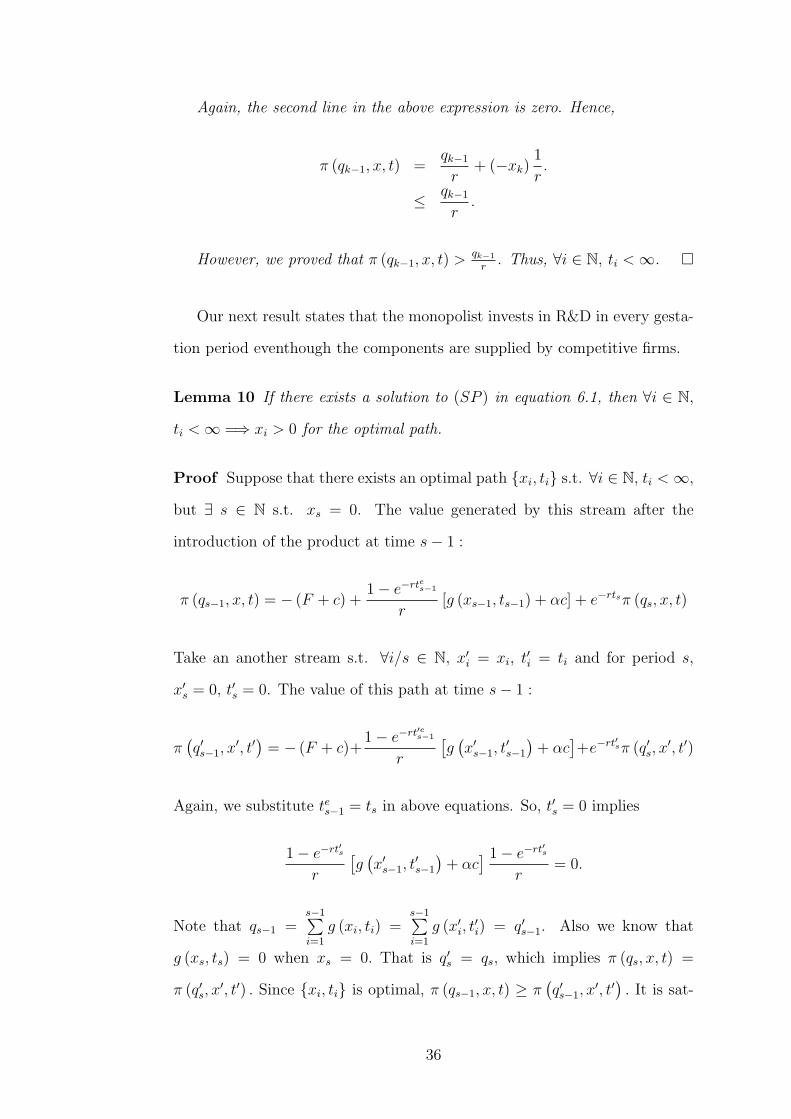
Our next result states that the monopolist invests in R&D in every gesta-

tion period eventhough the components are supplied by competitive firms.

Lemma 10 If there exists a solution to (SP ) in equation 6.1, then ∀i ∈ N,

ti < ∞ =⇒ xi > 0 for the optimal path.

Proof Suppose that there exists an optimal path {xi, ti} s.t. ∀i ∈ N, ti < ∞,

but ∃ s ∈ N s.t. xs = 0. The value generated by this stream after the

introduction of the product at time s− 1 :

π (qs−1, x, t) = − (F + c) +1− e−rtes−1

r[g (xs−1, ts−1) + αc] + e−rtsπ (qs, x, t)

Take an another stream s.t. ∀i/s ∈ N, x′i = xi, t′i = ti and for period s,

x′s = 0, t′s = 0. The value of this path at time s− 1 :

π(q′s−1, x

′, t′)

= − (F + c)+1− e−rt′es−1

r

[g(x′s−1, t

′s−1

)+ αc

]+e−rt′sπ (q′s, x

′, t′)

Again, we substitute tes−1 = ts in above equations. So, t′s = 0 implies

1− e−rt′s

r

[g(x′s−1, t

′s−1

)+ αc

] 1− e−rt′s

r= 0.

Note that qs−1 =s−1∑i=1

g (xi, ti) =s−1∑i=1

g (x′i, t′i) = q′s−1. Also we know that

g (xs, ts) = 0 when xs = 0. That is q′s = qs, which implies π (qs, x, t) =

π (q′s, x′, t′) . Since {xi, ti} is optimal, π (qs−1, x, t) ≥ π

(q′s−1, x

′, t′). It is sat-

36

isfied when

1− e−rts

r[g (xs−1, ts−1) + αc] +

(e−rts − 1

)π (qs, x, t) ≥ 0

That is either

ts = 0

or (π (qs, x, t)− [g (xs−1, ts−1) + αc]

r

)≤ 0. (6.2)

By Lemma 9 above, π (qs, x, t) > qs

r. Moreover, qs = qs−2 + g (xs−1, ts−1) +

g (xs, ts) where g (xs, ts) = 0. If we substitute this into equation 6.2, we obtain:

αc

r>

qs−2

r

However, by Assumption 3, pc (g, q, αc) ≤ q, in case αc ≤ qs−2. Hence, ts = 0.

π (qs−1, x, t) = − (F + c) + e−rtsπ (qs, x, t)

< π (qs, x, t)

Since g (xs, ts) = 0 , π (qs−1, x, t) = π (qs, x, t). Thus we have a contradiction.

If {xi, ti} is an optimal path and ∀i ∈ N, ti < ∞, then ∀i ∈ N, xi > 0. �

Given the above we can now show there is a solution to the monopolist’s

problem when there is perfect competition in the component market.

Proposition 3 There exists a global maximum to the monopolist’s problem.

37

Proof The profit function for the selling monopolist is

π (q0, x, t) =q0

r+ (−x1)

1− e−rt1

r

+∞∑i=1

e−rTi (g (xi, ti) + αc)1− e−rtei

r

+∞∑i=1

e−rTi

[− (F + c)− xi+1

1− e−rti+1

r

]

Note that ∀i ∈ N, g (xi, ti) is bounded. So, for some j ∈ N, π (q0, x, t) →

−∞ as xj → ∞. That is for some X, π (q0, x, t) < 0, ∀xi > X. However,

we established in Lemma 9 that π (q0, x, t) > q0

r. Hence, xi’s must be chosen

from [0, X] . Also, for some j ∈ N, as tj → ∞, π (q0, x, t) < π (q0, x, t) +

π (qj−1, xp, tp) = π′ where π (qj−1, xp, tp) is the profit generated by a constant

stream {xp, tp} after the introduction of the product of quality qj−1. However,

we know that π (qj−1, xp, tp) >qj−1

r. This implies for some T, π (q0, x, t) < π′,

∀ti > T. So, ti’s must be chosen from [0, T ] . Hence, the maximum must be

within the compact domain [0, X]× [0, T ] .

Since g is continuous, π is continuous. π is continuous within the compact

domain [0, X] × [0, T ]. So, it has a maximum. By Lemma 10, we have an

interior solution. �

Let π∗C be a solution to the sequential problem when the component mar-

ket is perfectly competitive. We establish again the corresponding functional

equation,

(FE) Π (q) = maxx,t

{−1

rx + e−rt

(− (F + c) +

x

r+ p (q, x, t) + Π (q′)

)}(6.3)

where p (q, x, t) = (g + αc) 1−e−rte

r.

As we did before, we will show now the sequential problem and the func-

tional equation have the same solutions.

38

Lemma 11 π∗C solves (FE) in equation 6.3.

Proof Q, A, H, > are defined as before. The objective function in equation

6.1 can also be written as follows:

π (q0, x, t) =q0

r+

∞∑i=1

e−rTi−1e−rti (g (xi, ti) + αc)(1− e−rti+1)

r(6.4)

+∞∑i=1

e−rTi−1

[−e−rti (F + c)− xi

1− e−rti

r

](6.5)

Then, we have following form for the sequential problem in equation 6.4:

π (q0, x, t) =q0

r+

∞∑i=1

βiHi where

βi = e−rTi−1 and

Hi = −xi1− e−rti

r+ e−rti

((g (xi, ti) + αc)

(1− e−rti+1)

r− (F + c)

)

Again, since > (qi) = qi + g (xi+1, ti+1) = qi+1 for each i ∈ N, Q is a convex

subset of R, and the correspondence > : Q → Q is nonempty, compact-valued

and continuous. For each i ∈ N, 0 < βi < 1. Also, g is bounded and ∀i ∈ N,

(xi, ti) ∈ [0, X] × [0, T ]. Hence, Hi is bounded for each i ∈ N. Since g is

continuous, Hi is continuous. With conditions above satisfied, solutions to

(FE) coincide exactly to solutions of (SP ) (Stokey, 1989). �

We can now continue our analysis with functional equation. In order to

analyze how R&D incentives are affected when the market structure in the

component market changes, we should look at the first order conditions.

Lemma 12 Π is continuously differentiable at q. Moreover, Πq (q) is zero.

Proof The proof of differentiability is similar to the one in Chapter 5. By

Assumption 3, H is strictly concave (see the appendix). Since g and pc are

continuously differentiable, so is H. As we stated before, > is convex. Hence,

39

Π is continuously differentiable at q (Stokey, 1989).

Πq (q) = Πq1 (q1) = e−rt1 (pq1 (q, x, t) + Πq2 (q2))

=∞∑i=1

e−r

(i∑

j=0tj

)pqi

(q, x, t) where t0 = 0.

However, since p (q, x, t) = (g + αc) 1−e−rte

r, pqi

(q, x, t) = 0 for each i ∈ N.

That is Πq (q) = 0. �

Above lemma states that when the component market is perfectly com-

petitive, the quality of a product does not affect monopolist’s profits. This

is different than what we find in the case where the monopolist controls the

component market. Since there is now competition in the component mar-

ket, the monopolist can not charge the flow utility of the current product for

the price of the component. Therefore, the price of the new generation is

now determined by three factors; g− quality increment between two consecu-

tive products, te− consumers’ expectations and αc− the marginal cost of the

component.

Π satisfies the following first order conditions:

Πx = −(1− e−rt)

r+ e−rt ∂p (q, x, t)

∂x

+e−rt ∂p (q, x, t)

∂qgx + e−rt ∂Π (q′)

∂q′gx (6.6)

Πt = −re−rt(− (F + c) +

x

r+ p (q, x, t) + Π (q′)

)+e−rt

(∂p (q, x, t)

∂t+

∂p (q, x, t)

∂qgt +

∂Π (q′)

∂q′gt

)(6.7)

If we substitute pq (q, x, t) = 0 and Πq (q) = 0 into equations 6.6 and 6.7,

we obtain

40

−(1− e−rt)

r+ e−rt 1− e−rt

rgx = 0 (6.8)

r (F + c)− x− rp (q, x, t)− rΠ (q′) +1− e−rt

rgt = 0 (6.9)

First order conditions for the monopoly are different when there is perfect

competition in the component market. There is an extra term (1− e−rt) mul-

tiplied by e−rt gx

rand gt

r. This implies marginal productivities of R&D inputs

are less effective on monopoly profits if the environment in the component

market becomes competitive. The reason is as follows: R&D inputs affect

the prices of the later generations in two ways. The direct effect is that R&D

investments determine the level of the quality increment, g, thereby affecting

immediately the price of the next generation. The indirect effect is that since

knowledge builds up cumulatively, they determine the quality of the next

product, which affects the price of the component in later generations. When

the monopolist controls the component market, these two effects are active.

However, if the component market is perfectly competitive, the indirect effect

is eliminated as the price of the component is always set up at its marginal

cost.

We are not able to analyze the optimal choices of x and t just solving

these first order conditions. However, in the next chapter we will also be

able to determine how gestation periods and R&D investments change if the

competition arises in the component market.

Our analysis in this chapter coincide with Fishman and Rob’s monopoly

analysis for slightly different costs. They find the monopolist innovates less

frequently and invests less in R&D than the social planner. In the next chap-

ter, we are going to show that the market structure of the component market

changes these results even the monopolist can engage in partial physical ob-

solescence.

41

CHAPTER 7

THE EQUILIBRIUM WHEN THE

COMPONENT MARKET IS

IMPERFECTLY COMPETITIVE

We now consider the case where the component market is imperfectly com-

petitive. In Chapter 5, we find that if the monopolist has full market power

in the component market, the optimal price for the component good is the

quality of the current product in flow terms. In Chapter 6, if the component

market is perfectly competitive, the price of the component good is set up at

its marginal cost, αc. Accordingly, we assume that if the component market

is imperfectly competitive, the price of the component lies between these two

values. Since there is now competition in the component good market, the

monopolist can not charge q for the component good and also we rule out the

case where pc ≤ αc, thereby preventing firms making loss in the component

market. Therefore, pc ∈ (αc, q) and the corresponding sequential problem for

the monopolist is

(SP ) sup{xi,ti}∞i=1

π (q0, x, t) s.t.

42

π (q0, x, t) =q0

r+ (−x1)

1− e−rt1

r

+∞∑i=1

e−rTi [g (xi, ti) + pc (g, qi, αc)]1− e−rtei

r

+∞∑i=1

e−rTi

[− (F + c)− xi+1

1− e−rti+1

r

](7.1)

Note that when for each i ∈ N, pc (g, qi, αc) = qi, we have the same

problem when the monopolist controls the component market. When for

each i ∈ N, pc (g, qi, αc) = αc, we ended up with the monopolist’s problem in

Chapter 6, where the monopolist faces perfect competition in the component

market.

We are going to follow the same steps as we did in previous chapters.

Lemma 13 For any given path {xi, ti}∞i=1, π (q0, x, t) < ∞. Furthermore, if

{xi, ti}∞i=1 is an optimal path, then q0

r< π (q0, x, t) and ∀i ∈ N, ti < ∞.

Proof Since for each i ∈ N, pc (g, qi, αc) < qi, for any path {xi, ti}∞i=1

π (q0, x, t) < W (q0, x, t) .

We proved in Lemma 1 that for any given path {xi, ti}∞i=1, W (q0, x, t) <

∞. Hence, π (q0, x, t) < ∞.

Now, suppose that {x∗i , t∗i } solves (SP ) . Let πIMp be the value of the con-

stant stream in imperfect component market, which is ∀i ∈ N, {xi, ti} =

{xp, tp}. Hence,

πIMp =

q0 − xp

r+

g (xp, tp)(1− e−rte

)r (ertp − 1)

+∞∑i=1

e−ritp(1− e−rte

)pc (qi, αc)

r− (F + c)

ertp − 1

Now, for each i ∈ N, αc ≤ pc (g, qi, αc). Thus, πCp ≤ πIM

p , where πCp be

43

the value of the constant stream in perfectly competitive component market.

By Lemma 9, πIMp > q0

r. Since {x∗i , t∗i } solves (SP ) , the value generated

by the stream {x∗i , t∗i } must be at least equal to any other stream. That is

π∗ (q0, x∗, t∗) ≥ πIM

p > q0

r.

In order to prove the final step, suppose that there exists an optimal path

{xi, ti} such that for some period k, tk = ∞. The value of the stream after

the introduction of the product of quality qk−1,

π (qk−1, x, t) =qk−1

r+ (−xk)

1− e−rtk

r

+∞∑

i=k

e−rTi [g (xi, ti) + pc (qi, αc)]1− e−rtei

r

+∞∑

i=k

e−rTi

[− (F + c)− xi+1

1− e−rti+1

r

]

As before, second line in the above expression is zero. Hence,

π (qk−1, x, t) =qk−1

r+ (−xk)

1

r.

≤ qk−1

r.

However, we know that π (qk−1, x, t) > qk−1

r. Thus, ∀i ∈ N, ti < ∞. �

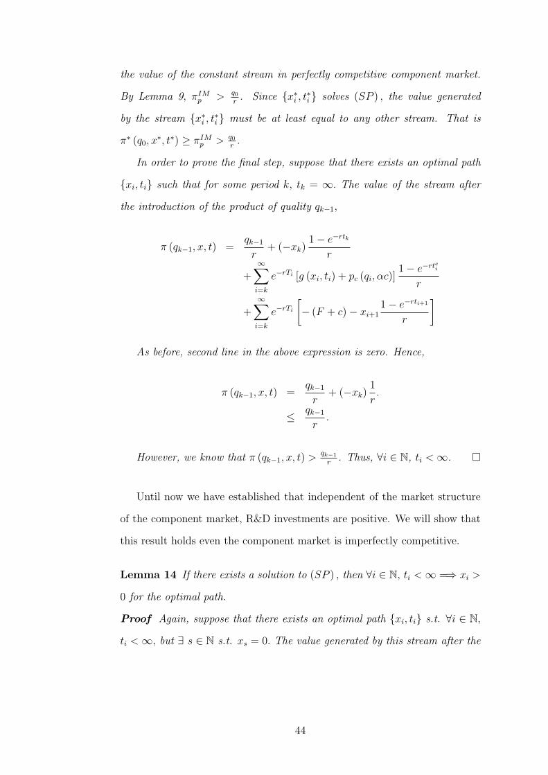
Until now we have established that independent of the market structure

of the component market, R&D investments are positive. We will show that

this result holds even the component market is imperfectly competitive.

Lemma 14 If there exists a solution to (SP ) , then ∀i ∈ N, ti < ∞ =⇒ xi >

0 for the optimal path.

Proof Again, suppose that there exists an optimal path {xi, ti} s.t. ∀i ∈ N,

ti < ∞, but ∃ s ∈ N s.t. xs = 0. The value generated by this stream after the

44

introduction of the product at generation s− 1 :

π (qs−1, x, t) = − (F + c) +1− e−rtes−1

r[g (xs−1, ts−1) + pc (g, q, αc)]

+e−rtsπ (qs, x, t)

Take an another stream s.t. ∀i/s ∈ N, x′i = xi, t′i = ti and for period s,

x′s = 0, t′s = 0. The value of this path at time s− 1 :

π(q′s−1, x

′, t′)

= − (F + c) +1− e−rte

′s−1

r

[g(x′s−1, t

′s−1

)+ pc (g, q′, αc)

]+e−rt′sπ (q′s, x

′, t′)

Substituting tes−1 = ts and t′s = 0, we obtain

1− e−rt′s

r

[g(x′s−1, t

′s−1

)+ pc (g, q′, αc)

]= 0.

Again, q′s = qs implies π (qs, x, t) = π (q′s, x′, t′). Since {xi, ti} is optimal,

π (qs−1, x, t) ≥ π(q′s−1, x

′, t′). It is satisfied when

1− e−rts

r[g (xs−1, ts−1) + pc (g, q, αc)] +

(e−rts − 1

)π (qs, x, t) ≥ 0

That is either

ts = 0

or

π (qs, x, t) ≤ g (xs−1, ts−1) + pc (g, q, αc)

r. (7.2)

We know that at time s − 1, pc (g, q, αc) < qs−2. Equation 7.2 is satisfied

when

π (qs, x, t) <qs

r

45

However, by Lemma 13 above, π (qs, x, t) > qs

r. Thus, ts = 0 and

π (qs−1, x, t) = − (F + c) + e−rtsπ (qs, x, t)

< π (qs, x, t)

Since g (xs, ts) = 0, π (qs−1, x, t) = π (qs, x, t). Thus, we have a contradiction.

�

Proposition 4 There exists a global maximum to the monopolist’s problem.

Proof See the proof of Proposition 2. �

Let π∗IM be a solution to (SP ) . We now establish the functional equation

for the monopolist’s problem as we did in previous chapters,

(FE) Π (q) = maxx,t

{−1

rx + e−rt

(− (F + c) +

x

r+ p (q, x, t) + Π (q′)

)}(7.3)

where p (q, x, t) = (g + pc (g, q, αc)) 1−e−rte

r.

Lemma 15 π∗IM solves (FE) in equation 7.3.

Proof See the corresponding lemma when the monopolist controls the com-

ponent market. �

In order to prove our main proposition, we need the following lemma.

Lemma 16 Π is continuously differentiable at q.

Proof Similar to the corresponding lemma in Chapter 5. Note that

Πq (q) = Πq1 (q1) = e−rt1 (pq1 (q, x, t) + Πq2 (q2))

=∞∑i=1

e−r

(i∑

j=0tj

)pqi

(q, x, t) where t0 = 0.

46

Since p (q, x, t) = (g + pc (g, q, αc)) 1−e−rte

r, pqi

(q, x, t) = pcq (g, q, αc) 1−e−rtei

r

for each i ∈ N. Hence,

Πq (q) =∞∑i=1

e−r

(i∑

j=0tj

)pcq (g, q, αc)

1− e−rtei

r(7.4)

�

Π satisfies the following first order conditions:

Πx = −(1− e−rt)

r+ e−rt ∂p (q, x, t)

∂x

+e−rt ∂p (q, x, t)

∂qgx + e−rt ∂Π (q′)

∂q′gx (7.5)

Πt = −re−rt(− (F + c) +

x

r+ p (q, x, t) + Π (q′)

)+e−rt

(∂p (q, x, t)

∂t+

∂p (q, x, t)

∂qgt +

∂Π (q′)

∂q′gt

)(7.6)

Now, we are going to analyze the direction of changes in R&D decisions

when the price of the component good increases. In this way, we will be able

to figure out how the market structure of the component market affects the

innovation activity.

Proposition 5 If the price of the component increases, the selling monopolist

innovates more frequently and invests more in R&D.

Proof We know from first order conditions in equations 7.5 and 7.6,

Πt (q) = 0

Πx (q) = 0

47

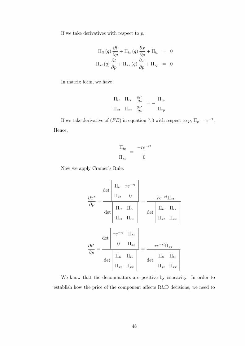
If we take derivatives with respect to p,

Πtt (q)∂t

∂p+ Πtx (q)

∂x

∂p+ Πtp = 0

Πxt (q)∂t

∂p+ Πxx (q)

∂x

∂p+ Πxp = 0

In matrix form, we have

Πtt Πtx

Πxt Πxx

∂t∗

∂p

∂x∗

∂p

= −Πtp

Πxp

If we take derivative of (FE) in equation 7.3 with respect to p, Πp = e−rt.

Hence,

Πtp

Πxp

=−re−rt

0

Now we apply Cramer’s Rule.

∂x∗

∂p=

det

∣∣∣∣∣∣∣Πtt re−rt

Πxt 0

∣∣∣∣∣∣∣det

∣∣∣∣∣∣∣Πtt Πtx

Πxt Πxx

∣∣∣∣∣∣∣=

−re−rtΠxt

det

∣∣∣∣∣∣∣Πtt Πtx

Πxt Πxx

∣∣∣∣∣∣∣

∂t∗

∂p=

det

∣∣∣∣∣∣∣re−rt Πtx

0 Πxx

∣∣∣∣∣∣∣det

∣∣∣∣∣∣∣Πtt Πtx

Πxt Πxx

∣∣∣∣∣∣∣=

re−rtΠxx

det

∣∣∣∣∣∣∣Πtt Πtx

Πxt Πxx

∣∣∣∣∣∣∣We know that the denominators are positive by concavity. In order to

establish how the price of the component affects R&D decisions, we need to

48

figure out the signs of Πxt and Πxx. Since

Πx = −(1− e−rt)

r+ e−rt ∂p (q, x, t)

∂x+ e−rt ∂p (q, x, t)

∂qgx + e−rt ∂Π (q′)

∂q′gx

= −(1− e−rt)

r+ e−rt 1− e−rte

rgx

+e−rt 1− e−rte

r

∂pc (g, q, αc)

∂qgx + e−rt ∂Π (q′)

∂q′gx

Πxx = e−rt

1−e−rte

rgxx + 1−e−rte

rpcq (g, q, αc) gxx + 1−e−rte

rpcqq (g, q, αc) (gx)

2

+ Πq′ (q′) gxx + Πq′q′ (q

′) (gx)2

Under Assumptions 3 and 3, we have pcq (g, q, αc) > 0, pcqq (g, q, αc) ≤ 0

and gxx ≤ 0. Moreover, equation 7.4 implies Πq′q′ (q′) ≤ 0 and Πq′ (q

′) > 0.

Thus, Πxx < 0.

Πxt = −e−rtr

(1

r+

1− e−rte

rgx +

1− e−rte

rpcq (g, q, αc) gx + Πq′ (q

′) gx

)

+e−rt

1−e−rte

rgxt + 1−e−rte

rpcq (g, q, αc) gxt

+1−e−rte

rpcqq (g, q, αc) gxgt

+e−rt (Πq′ (q

′) gxt + Πq′q′ (q′) gxgt)

If we rearrange the terms, we have

Πxt = e−rt

−1 + 1−e−rte

r(gxt − rgx) + 1−e−rte

rpcq (g, q, αc) (gxt − rgx)

+Πq′ (q′) (gxt − rgx)

+ 1−e−rte

rpcqq (g, q, αc) gxgt + Πq′q′ (q

′) gxgt

If x and t are substitutes- gxt < 0 for all (x, t)−or if x and t are comple-

ments but not strong complements- 0 < gxt < rgx, the term in parenthesis

would be negative. As Fishman and Rob (2000) state some conventional

49

productions functions, such as Cobb-Douglas or the constant elasticity of

substitution satisfy this condition. Hence, we assume this restriction on g

holds.

Thus, Πxt < 0.

Therefore,

∂x∗

∂p

1− e−rte

r=

∂x∗

∂pc

> 0 (7.7)

and

∂t∗

∂p

1− e−rte

r=

∂t∗

∂pc

< 0 (7.8)

�

From Proposition 5, one can easily show the following results.

Corollary 1 The monopolist innovates less frequently and invests less in

R&D than the efficient level unless he controls the component market.

Corollary 2 Competition in the component good market causes efficiency

loss in terms of R&D investments.

The results state that if the price of the component is higher, the mo-

nopolist innovates more frequently and invests more in R&D. The reason is

that consumers are willingly to pay for the incremental quality improvement

when a new generation is introduced. This implies the monopolist receives

less than the social value of an innovation. However, if the monopolist is able

to determine the durability of the component, he receives the social value

of an innovation by increasing the price of the component, which consumers

have to replace. It can charge as high as possible for the price of the compo-

nent when he controls the component market. On the other hand, when the

component market is imperfectly competitive, he is not able to compensate

his loss by changing the price of the component, thus he waits longer between

two product introductions. Thereby, consumers pay for the present model

in a longer period, which leads innovations to be delayed.

50

Different than Fishman and Rob (2000), our results depend on the market

structure of the component market. We find that the monopolist innovates

less frequently and invests less in R&D than the efficient level unless he con-

trols the component market. Incorporating the component durability enables

us to conclude that competition in the component market causes departures

form socially optimal level of R&D investments. Therefore, a monopolist in

a primary market should also have market power in its component market.

We examine now how current R&D decisions change when the price of

the component good increases in the future.

Proposition 6 If the price of the component increases in the future, the

monopolist innovates less frequently and invests less in R&D today.

Proof Assume that at time s − 1, the monopolist has to decide its R&D

inputs, xs and ts. Let the price of the component be pck after k generations.

Πts (q) = 0

Πxs (q) = 0

If we take derivatives with respect to pk,

Πtt (q)∂ts∂pk

+ Πtx (q)∂xs

∂pk

+ Πtpk= 0

Πxt (q)∂ts∂pk

+ Πxx (q)∂xs

∂pk

+ Πxpk= 0

In matrix form, we have

Πtt Πtx

Πxt Πxx

∂ts∂pk

∂xs

∂pk

= −Πtpk

Πxpk

Now, if we take derivative of Π with respect to pk at time s−1, we obtain

Πpk= Πk

i=se−rti

51

Hence,

Πtpk

Πxpk

=−rΠk

i=se−rti

0

Again we apply Cramer’s Rule.

∂xs

∂pk

=

det

∣∣∣∣∣∣∣Πtt −rΠk

i=se−rti

Πxt 0

∣∣∣∣∣∣∣det

∣∣∣∣∣∣∣Πtt Πtx

Πxt Πxx

∣∣∣∣∣∣∣=

rΠki=se

−rtiΠxt

det

∣∣∣∣∣∣∣Πtt Πtx

Πxt Πxx

∣∣∣∣∣∣∣

∂ts∂pk

=

det

∣∣∣∣∣∣∣−rΠk

i=se−rti Πtx

0 Πxx

∣∣∣∣∣∣∣det

∣∣∣∣∣∣∣Πtt Πtx

Πxt Πxx

∣∣∣∣∣∣∣=−rΠk

i=se−rtiΠxx

det

∣∣∣∣∣∣∣Πtt Πtx

Πxt Πxx

∣∣∣∣∣∣∣We have Πxt < 0 and Πxx < 0. Therefore,

∂xs

∂pk

1− e−rte

r=

∂xs

∂pck

< 0 (7.9)

and

∂ts∂pk

1− e−rte

r=

∂ts∂pck

> 0

�

52

CHAPTER 8

CONCLUSION

Early work in durable goods theory has always suggested that planned obso-

lescence is an incentive to reduce the durability of the whole of the product.

However, usually it is a component that becomes physically obsolete rather

than the whole unit.

In this paper, we analyze the R&D investments and the frequency of prod-

uct innovations of a durable good monopoly under the assumption that the

monopolist determines the durability of the component. We study the ef-

fects of the market structure in the component market on R&D decisions of

a durable good monopolist. We extend Fishman and Rob’s analysis by incor-

porating partial physical obsolescence to the model. The main assumptions

of the model are; innovations are recurrent, the knowledge builds up cumula-

tively, consumers are homogenous and the monopolist sells rather than rent

its products. We showed that under these circumstances if the monopolist

has market power in the component market, he innovates at the socially op-

timal pace. However, if the component market is perfectly competitive, the

monopolist innovates less frequently and invests less than the efficient level.

Our results in the case of perfectly competitive component market is similar

to Fishman and Rob’s.

We should note that the price structure different than the one in our

53

analysis may change the results. However, incorporating more complex price

structure to the model will complicate the analysis. In addition, allowing

the monopolist to rent its products or relaxing the consumer homogeneity

assumption may strengthen or weaken our results. The analysis of these

issues is going to be the topic of future research.

54

BIBLIOGRAPHY

Bond, E.W., and Samuelson,L. 1987. “Durable Goods, Market Structureand the Incentives to Innovate,” Economica 54: 57-67.

Borenstein, S., Mackie-Mason, J.K., and Netz, J. 2000. “Exercising MarketPower in Proprietary Markets,” Journal of Economics&ManagementStrategy 9: 157-188.

Bulow, J. 1982. “Durable-Goods Monopolists,” Journal of Political Econ-omy 90: 314-332.

Bulow, J. 1986. “An Economic Theory of Planned Obsolescence,” TheQuarterly Journal of Economics 42: 729-748.

Chen, Z.,and Ross,T.W. 1998. “Orders to supply as substitutes forcommitments to aftermarkets,” Canadian Journal of Economics 31:1204-24.

Chen, Z.,and Ross,T.W. 1998. “Refusals to deal and orders to supply incompetitive markets,” International Journal of Industrial Organization17: 399-417.

Choi, J.P. 1994. “Network Externality, Compatibility Choice, and PlannedObsolescence,” The Journal of Industrial Economics 42: 167-182.

Coase, R. 1972. “Durability and Monopoly,” Journal of Law and Economics15: 143-149.

Fishman, A.,and Rob, R. 2000. “Product Innovation by a Durable-GoodMonopoly,” RAND Journal of Economics 31: 237-252.

Kumar, P. 2000. “Price and Quality Discrimination in Durable GoodsMonopoly with Resale Trading,” International Journal of IndustrialOrganization 20: 1313-1339.

55

Lucas, R.E.,and Stokey, N.L. 1989. Recursive Methods in EconomicDynamics. Cambridge: Harvard University Press.

Marinoso, B.G. 2001. “Technological Incompatibility, Endogenous Switch-ing Costs and Lock-In,” The Journal of Industrial Economics 49:281-294.

Rust, J. 1986. “When Is It Optimal to Kill off the Market for Used DurableGoods,” Econometrica 54: 65-86.

Shapiro, C.,and Teece, D.J. 1994. “Systems Competition and Aftermarkets:An Economic Analysis of Kodak,” Antitrust Bulletin 39: 135-162.

Swan, P.L. 1972. “Optimum Durability, Second-Hand Markets, andPlanned Obsolescence,” Journal of Political Economy 80: 575-585.

Waldman, M. 1993. “A New Perspective on Planned Obsolescence,” TheQuarterly Journal of Economics 108: 273-283.

Waldman, M. 1996. “Planned Obsolescence and the R&D Decision,”RAND Journal of Economics 27: 583-595.

56

APPENDIX

Proof [Proof of Lemma 5] In order to prove V is differentiable, we need to

prove first per period return function H is strictly concave. So, we are going

to show D2H (x, t) is a negative definite matrix.

D2H (x, t) =Hxx Hxt

Htx Htt

D2H (x, t) is negative definite if and only if Hxx < 0 and HxxHtt− HxtHtx >

0. Now, we will derive second order derivatives.

H = −x(1− e−rt)

r+ e−rt

(g (x, t)

r− (F + c)

)Hx = −(1− e−rt)

r+ e−rt gx

r= 0

Hxx = e−rt gxx

r

We assume that g is strictly concave. Hence, Hxx < 0.

Ht = −xe−rt − re−rt

(g (x, t)

r− (F + c)

)+ e−rt gt

r= 0

Htt = rxe−rt + r2e−rt

(g (x, t)

r− (F + c)

)− re−rt gt

r

−re−rt gt

r+ e−rt gtt

r

Htx = −e−rt − e−rtgx + e−rt gtx

r

Similarly,

Hxt = −e−rt − e−rtgx + e−rt gxt

r

57

We assume that gxt = gtx. This implies Hxt = Htx. We want to have dif-

ferentiability around the optimal solution so that we substitute first order

conditions into the second order conditions. This yields:

HxxHtt −H2xt = e−rt gxx

r

(−re−rt gt

r+ e−rt gtt

r

)−(−1 + e−rt gxt

r

)2

= −e−2rt gxx

rgt + e−2rt gxx

r

gtt

r−(−1 + e−rt gxt

r

)2

By Assumption 3, we have gxxgtt ≥ (gxt − rert)2. If we multiply both side

with e−2rt

r2 , we obtain

e−2rt gxx

r

gtt

r≥(e−rt gxt

r− 1)2

Since g is increasing in t, −e−2rt gxx

rgt > 0. Thus, HxxHtt −H2

xt > 0. So, H is

strictly concave and V is differentiable. �

Proof [Proof of Lemma 10] Again, we need to prove per period return func-

tion H is strictly concave.

D2H (x, t) =Hxx Hxt

Htx Htt

D2H (x, t) is negative definite if and only if Hxx < 0 and HxxHtt− HxtHtx >

0. We derive second order conditions.

H = −x(1− e−rt)

r+ e−rt

((1− e−rte

) g (x, t) + q

r− (F + c)

)Hx = −(1− e−rt)

r+ e−rt

(1− e−rte

) gx

r= 0

Hxx = e−rt(1− e−rte

) gxx

r

58

Since g is strictly concave, Hxx < 0.

Ht = 0 = −xe−rt − re−rt

((1− e−rte

) g (x, t) + q

r− (F + c)

)+e−rt

(1− e−rte

) gt

r

Htt = −rHt +−re−rt(1− e−rte

) gt

r+ e−rt

(1− e−rte

) gtt

r

Htx = −e−rt − e−rt(1− e−rte

)gx + e−rt

(1− e−rte

) gtx

r

Similarly,

Hxt = −e−rt − e−rt(1− e−rte

)gx + e−rt

(1− e−rte

) gxt

r

We assume that gxt = gtx. This implies Hxt = Htx. We again substitute first

order conditions into the second order conditions. This yields:

HxxHtt −H2xt = e−2rt

(1− e−rte

)2 gxx

r

(−gt +

gtt

r

)−(e−rt

(1− e−rte

) gxt

r− 1)2

= −e−2rt(1− e−rte

)2 gxx

rgt + e−2rt

(1− e−rte

)2 gxx

r

gtt

r

−(e−rt

(1− e−rte

) gxt

r− 1)2

By Assumption 3, we have(1− e−rte

)2gxxgtt ≥

((1− e−rte

)gxt − rert

)2. If

we multiply both side with e−2rt

r2 , we get

e−2rt(1− e−rte

)2 gxx

r

gtt

r≥(e−rt

(1− e−rte

) gxt

r− 1)2

Thus, HxxHtt −H2xt > 0. H is strictly concave and Π is differentiable. �

Proof [Proof of Lemma 17] The proof is similar to the one above. The only

difference is in the formation of per period function H, q is replaced with αc.

�

59