product mix and earnings volatility at commercial banks...
TRANSCRIPT
Product Mix and Earnings Volatility atCommercial Banks: Evidence froma Degree of Leverage ModelRobert DeYoung and Karin P. Roland
Working Papers SeriesResearch Department(WP-99-6)
Federal Reserve Bank of Chicago
Working Paper Series
Product Mix and Earnings Volatility at Commercial Banks:Evidence from a Degree of Leverage Model
Robert DeYoungEconomic Research Department
Federal Reserve Bank of Chicago230 South LaSalle Street
Chicago, IL 60604312-322-5396
Karin P. RolandDepartment of Accounting and Finance
College of Business AdministrationValdosta State University
Valdosta, GA 31698912-293-6062
March 1999
______________________________________________________________________________The authors thank Eli Brewer, Rick Eichhorn, Doug Evanoff, Fred Furlong, Julapa Jagtiani, George Kaufman,Simon Kwan, David Marshall, Jim Moser, Francois Velde, and Larry Wall for their comments on earlier drafts ofthis paper. The opinions expressed herein are those of the authors, and do not necessarily reflect the views of theFederal Reserve Bank of Chicago, the Federal Reserve System, or their staffs.

Product Mix and Earnings Volatility at Commercial Banks:Evidence from a Degree of Leverage Model
Robert DeYoung, Federal Reserve Bank of ChicagoKarin P. Roland, Valdosta State University
March 1999
Abstract: Commercial banks’ lending and deposit-taking business has declined in recent years. Deregulation and new technology have eroded banks’ comparative advantages and made it easier fornonbank competitors to enter these markets. In response, banks have shifted their sales mix towardnoninterest income — by selling ‘nonbank’ fee-based financial services such as mutual funds; bycharging explicit fees for services that used to be ‘bundled’ together with deposit or loan products;and by adopting securitized lending practices which generate loan origination and servicing feesand reduce the need for deposit financing by moving loans off the books.
The conventional wisdom in the banking industry is that earnings from fee-based products aremore stable than loan-based earnings, and that fee-based activities reduce bank risk via diversification. However, there are reasons to doubt this conventional wisdom a priori. Compared to fees fromnontraditional banking products (e.g., mutual fund sales, data processing services, mortgage servicing),revenue from traditional relationship lending activities may be relatively stable, because switching costsand information costs reduce the likelihood that either the borrower or the lender will terminate therelationship. Furthermore, traditional lending business may employ relatively low amounts ofoperating and/or financial leverage, which will dampen the impact of fluctuations in loan-based revenueon bank earnings.
We test this conventional wisdom using data from 472 U.S. commercial banks between 1988and 1995, and a new ‘degree of total leverage’ framework which conceptually links a bank’s earningsvolatility to fluctuations in its revenues, to the fixity of its expenses, and to its product mix. Unlikeprevious studies that compare earnings streams of unrelated financial firms, we observe various mixesof financial services produced and marketed jointly within commercial banks. Thus, the evidence thatwe present reflects the impact of production synergies (economies of scope) and marketing synergies(cross-selling) not captured in previous studies. To implement this framework, we modify standarddegree of leverage estimation methods to conform with the characteristics of commercial banks.
Our results do not support the conventional wisdom. As the average bank tilts its product mixtoward fee-based activities and away from traditional lending activities, we find that the bank’s revenuevolatility; its degree of total leverage, and the level of its earnings all increase. The first two resultsimply increased earnings volatility (because earnings volatility is the product of revenue volatility andthe degree of total leverage) and the third result implies a possible risk premium.
These results have implications for bank regulators, who must set capital requirements at levelsthat balance the volatility of bank earnings against the probability of bank insolvency. These resultsalso suggest another explanation for the shift toward fee-intensive product mixes: a belief by bankmanagers that increased earnings volatility will enhance shareholder value (or at least will increase thevalue of the managers’ call options on their banks’ stock). Our results have no direct implications forthe expanded bank powers debate — we examine only currently permissible fee-based activities, andthese activities may have demand and production characteristics different from insurance underwriting,investment banking, or real estate brokerage.
Kaufman and Mote (1994) show that noninterest income comprised an even larger percentage of operating1
income at U.S. commercial banks during the 1930s and 1940s, due largely to the historically low demand forcommercial loans during the Depression and war years.
See DeYoung (1994) for levels and trends of noninterest income at large versus small banks. For analyst2
opinions regarding the importance of fee income for small bank profitability, see Anat Bird, “Industry Can’tCompete Without Off-Balance-Sheet Opportunities,” American Banker, May 25, 1995, and Karen Shaw Petrou,“New Business Lines May Be Small Banks’ Salvation,” American Banker, June 26, 1998.
1
Introduction
Commercial banks’ market share of loans and deposits has been in decline since the early
1980s. These trends — documented and analyzed by Boyd and Gertler (1994), Kaufman and Mote
(1994), Berger, Kashyap, and Scalise (1995), Edwards and Mishkin (1995), and others — were set in
motion by the elimination of decades-old regulatory restrictions that limited competition in banking
product markets and geographic markets, and by advances in information technology that negated
some of commercial banks’ traditional comparative advantages. Banks have reacted to declining
shares of their most traditional business activities by increasing the production and sale of fee-based
financial services. Between 1984 and 1997, noninterest income at FDIC-insured commercial banks
increased from 25 percent to 38 percent of aggregate operating income (i.e., revenues net of interest
expenses). Although this shift toward fee-based activities has been more pronounced at larger1
institutions than at smaller banks, some bank analysts believe that fee income is the key to profitability
and survival for community banks. 2
Commercial banks have long earned noninterest income by offering ‘traditional’ banking
services such as checking, trust, and cash management. The recent increase in the importance of
noninterest income has come from several sources. First, banks have expanded into less traditional
fee-for-service products such as insurance and mutual fund sales, and (limited) investment banking
activities. Second, banks now charge explicit fees for a number of financial services which
traditionally had been bundled together with deposit accounts and which customers previously
had paid for by accepting lower interest rates on deposits. For example, retail customers might
receive higher interest rates on their deposits but have to pay explicit fees for visiting bank tellers,
The preceding quotations appeared in, respectively, the American Banker, May 30, 1997; American Banker, May3
30, 1997; American Banker, May 30, 1997; and Northwestern Financial Review, May 24, 1997.
2
and correspondent banking customers might now earn interest on their compensating balances but
have to pay explicit fees for data processing services. Third, the growth of securitization in
mortgage, credit card, and other loan markets has presented banks with opportunities to earn fee
income from originating and servicing loans separate from interest income earned by holding loans
on the books. Further expansions of fee-based activities are likely in the near future as the legal
barriers between commercial banking, investment banking, and insurance industries become more
blurred or disappear entirely.
The conventional wisdom among bankers, bank regulators, and bank analysts is that fee-based
earnings are more stable than loan-based earnings, chiefly because they are less sensitive to movements
in interest rates and to economic downturns. Furthermore, the general feeling is that adding fee-based
activities to a traditional mix of banking products will reduce earnings volatility via diversification
effects. Roger Fitzsimmons, the chairman of Firstar Corp., has stated that “there is a stability to [fee]
income that we like.” Banking analyst Richard X. Bove states that “Banks that have strong fee-based
business and that do not have major commitments to the loan sector can weather the storm much better
than those banks that are building a loan portfolio.” Andrew Hove, twice the Acting Chairman of the
FDIC, has stated that “the growth in the relative performance of noninterest income over the years
reflects a diversifying industry, were risks are being spread.” If these claims are true, banks that
produce broad mixes of financial services should be less risky, all else held equal, than pure financial
intermediaries. By extension, these arguments imply that further expansion of bank powers — to
underwrite securities and insurance, or to participate in markets ancillary to financial services such as
real estate brokerage or computer sales — would reduce further the riskiness of commercial banks.
With this in mind, former Comptroller of the Currency, Eugene Ludwig stated that insurance sales “is a
product that marries nicely with the banking business, is low risk, and should certainly be allowed.”3
There are a number of reasons, however, to doubt this conventional wisdom. First, banks can
The source of the mutual fund revenue figure is the American Banker, July 16, 1996. Note that from 19844
through 1997, the percentage of real estate loans held by commercial banks that were noncurrent (i.e., 90 days pastdue or no longer accruing) fluctuated only between 1.1 percent and 5.4 percent (source: OCC Quarterly Journal).
American Banker, January 26, 1998.5
3
have qualitatively different relationships with fee-based customers than with their traditional loan-based
customers. Revenue from a bank’s traditional lending activities is likely to be relatively stable over
time, because switching costs and information costs make it costly for either borrowers or lenders to
walk away from a lending relationship. Revenue from fee-based activities is more likely to fluctuate
from period to period, because banks face relatively high competitive rivalry, relatively low information
costs, and less stable demand in a number of these product markets (e.g., investment advice, mutual
fund and insurance sales, data processing services). For example, fee income in the banking industry
from mutual fund sales fell by about 50 percent in 1994, a short-run fluctuation in revenue that would
be unthinkable in the lending business where, even during an economic downturn, only a small
percentage of loans stop making interest payments.4
Second, the input mix needed to produce fee-based financial services can be quite different
from that needed to produce more traditional intermediation-based products. The key here is that a
high ratio of fixed-to-variable expenses increases the bank’s operating leverage, which turns any given
amount of volatility in revenues into an even greater amount of earnings volatility. Once a bank has
established a lending relationship with a customer, increasing the amount of credit actually extended
requires the bank to increase only its variable costs (interest expense), which reduces its operating
leverage. In contrast, expanding the production of certain fee-based services can require the bank to
hire additional fixed labor inputs, which increases its operating leverage. This point is underscored by
a quotation from a Standard & Poors analyst regarding J.P. Morgan & Co.: “Over the last decade, the
company’s business mix has evolved, so that it has become increasingly reliant on...underwriting,
advisory services, and trading. This profile has rendered earnings more volatile. The expense base has
also become quite high, so that earnings could be vulnerable to revenue declines.” 5
American Banker, December 21, 1994.6
4
Third, bank regulators do not require the bank to hold any capital against many fee-based
activities (see Spong 1994, page 76), and banks that take advantage of this can increase their returns to
equity. For example, a Dean Witter Reynolds analyst concluded that Mellon Bank Corp. redeemed
$160 million of its in preferred stock in the aftermath of purchasing securities giant Dreyfus Corp.
because the combined firms “...don’t need as much capital for their fee business as they have for the
spread business.” Although most banks will internally allocate some capital to these activities, the6
lack of a regulatory capital requirement suggests a higher degree of financial leverage -- and thus
earnings volatility -- for these products.
Finally, there is evidence from the academic literature. Over the past two decades, a
substantial number of studies have investigated whether a repeal or revamp of the Glass-Steagall Act
would allow commercial banks to reduce risk by diversifying into currently nonpermissible,
nontraditional financial services. Although most of these studies (which we review below) find that
combining banking and nonbank activities creates the potential for risk-reducing diversification, these
studies also find that some nonbank activities tend to increase bank risk; that the returns to
diversification quickly diminish; and that any risk reduction achieved via diversification can be undone
by taking other risks, such as increased financial leverage.
These observations lead us to reconsider the popularly held belief that increased fee-based
activity tends to reduce the volatility of earnings at commercial banks. We test this proposition using
quarterly revenue and earnings data from 472 U.S. commercial banks between 1988 and 1995, and a
‘degree of total leverage’ framework which conceptually links the volatility of a bank’s earnings to its
revenue volatility, its expense fixity, and its product mix. To our knowledge, this is the first study to
use degree of leverage concepts to analyze risk at financial institutions. We devise a new empirical
framework based on these theoretical concepts, and we also modify standard degree of leverage
estimation techniques to make them compatible with the operational, financial, and strategic
5
characteristics of banks. These innovations allow us to investigate more completely than in previous
studies the manner in which alterations in product mix can affect the riskiness of financial institutions.
Most previous studies measure correlations between the earnings streams of pairs of financial services
produced by two unrelated firms, or produced by two affiliates of a financial services holding company
that are related only by common ownership. In contrast, we observe combinations of financial services
that are jointly produced and marketed within the same commercial bank, and because of this we
capture both cost synergies (scope economies) and revenue synergies (cross-selling) in our estimates of
the impact of product mix on earnings volatility.
Our results contradict the conventional wisdom. We find evidence that commercial bank
earnings grow more volatile as banks tilt their product mixes toward fee-based activities and away
from traditional intermediation activities. For the average bank in our sample, both revenue volatility
and the degree of total leverage increase with the share of bank revenue generated from non-deposit-
related, non-trading-related, fee-based activities. These two results imply that the volatility of bank
earnings increases as banks expand their fee-based activities because, as we show, earnings volatility is
the multiplicative product of revenue volatility and the degree of total leverage. We also find evidence
that the level of bank earnings increases as banks expand their fee-based activities, which suggests the
existence of a risk premium associated with these activities.
Our findings offer some (perhaps surprising) commentary on what two decades of changes in
competitive rivalry, technological advance, and business strategy in the commercial banking industry
have meant for the risk profiles of commercial banks. If, as seems likely, the share of commercial bank
revenues generated by fee-based activities continues to trend upward, our results imply that bank
earnings will become increasingly more volatile. Although most bank shareholders could neutralize the
effects of these changes on the riskiness of their portfolios by adjusting their holdings of nonbank
stocks, for bank regulators and bank managers the risks are less avoidable. Bank regulators bear only
the downside risk: holding capital constant, higher earnings volatility increases the probability that a
bank will become insolvent. Bank managers bear both the upside and the downside risk, and in some
6
circumstances may be attracted to especially volatile fee-based activities. Banks whose charter values
have eroded over the past twenty years now have less at risk, and shareholders may now prefer higher
earnings volatility in order to increase the upside probability of a large payout. Managers who own call
options on their bank’s stock may also prefer output mixes that generate high earnings volatility.
Although one might wish to use the results of this study to draw inferences about the wisdom
of various plans to allow commercial banks full brokerage and insurance underwriting powers, any
such inferences should be made with caution. On the one hand, we derive our results using an
empirical framework that captures production and marketing synergies across product lines,
phenomena that should be included in any benefit-cost analysis of whether banks should be allowed to
produce nontraditional services internally, at arms-length through a holding company, or not at all. On
the other hand, we derive our results from the revenues and earnings generated by fee-based activities
that are currently permissible for commercial banks, and this set of activities for the most part excludes
the securities and insurance activities central to the debate over expanded powers. Ultimately, the
degree to which our results are useful in this policy debate depends on the (unobserved) degree to
which the demand and production characteristics of the currently permissible fee-based activities are
similar to the characteristics of the proposed expanded powers.
The remainder of the paper is organized as follows. In section 1 we present a simple model of
the degree of total leverage at a multiproduct firm, and establish our research plan-of-attack. In section
2 we review the empirical literature on bank product mix and bank risk. In section 3 we describe our
data set, which contains quarterly observations of revenues and earnings for 472 sample banks between
1988 and 1995. In section 4 we compute revenue volatility for each of our sample banks, and discover
how revenue volatility varies across banks with different product mixes. In section 5 we modify
standard leverage estimation techniques for use on commercial bank data, use these techniques to
estimate the degree of total leverage for each of our sample banks, and then discover how the degree of
total leverage varies across banks with different product mixes. In section 6 we combine the
theoretical framework from section 1 with the empirical results from sections 4 and 5 to demonstrate
(1) DTL '
M
Mr(
r'
%% r
7
the degree to which earnings at the typical commercial bank are affected when product mix shifts away
from traditional lending activities and toward fee-based activities. In section 7 we summarize our main
results and discuss their implications for regulatory policy, business strategy, and future research.
1. Applying a Degree of Total Leverage Framework to Multiproduct Banking Firms
The concept of degree of total leverage summarizes the relationship between the top of a
business firm’s income statement (sales revenue) and the bottom of its income statement (earnings).
Consider a firm that has relatively high fixed expenses and relatively low variable expenses. We refer
to such a firm as being ‘highly levered’ or having a high ‘degree of leverage’. When sales revenues are
increasing at this firm, its earnings will increase more than proportionally, because a relatively large
portion of each additional revenue dollar can be retained due to the low variable expenses. Of course,
this sword has two edges -- when sales revenues are decreasing at a highly levered firm, losses will
occur more quickly due to its high fixed obligations. A firm's degree of total leverage (DTL) can be
defined as the percentage change in earnings () that is caused by a 1 percent change in revenue (r):
In other words, DTL is the ‘revenue elasticity of profits.’ Note that DTL can be expressed as the
product of two other leverage concepts, the degree of operating leverage and the degree of financial
leverage (i.e., DTL=DOL*DFL). DOL is the elasticity of earnings before interest and taxes (EBIT)
with respect to sales revenue, and reflects leverage in production. DFL is the elasticity of profits with
respect to EBIT, and reflects the use of financial leverage. Of the two concepts, financial leverage is
much more familiar in the banking industry, where financial liabilities often outnumber financial capital
by 10-to-1. (Ironically, in banking the ‘leverage ratio,’ defined as the ratio of book equity capital to
total assets, moves in the opposite direction from DFL.) We concentrate on DTL in this study because
changes in bank product mix can affect both operating and financial leverage, and because accurately
separating a bank’s interest expenses into operating costs and financing costs is difficult.
(2) % ' DTL ( % r
8
By rearranging the terms in (1) we can show that a high degree of total leverage can amplify a
given amount of revenue volatility (% r) into an even greater amount of earnings volatility (% ):
Assuming that the firm is a price taker in output markets, this formula decomposes earnings volatility
into two parts: volatility due to largely external market conditions (% r) and volatility due to internal
production and financing considerations (DTL).
Figure 1 shows how the degree of total leverage influences the relationship between bank
revenues and bank earnings. In the figure, Firm I is highly levered: it has high fixed costs (low vertical
intercept) and low variable costs (high slope). In contrast, Firm II is less highly levered: it has low
fixed costs (high vertical intercept) and high variable costs (low slope). Thus, for a given increase or
decrease in sales away from current revenue R , profits at Firm I vary more than do profits at Firm II. *
(Figure 1 assumes that increases and decreases in revenue are caused by fluctuations in quantity sold,
holding sales price constant.) Although increased revenue volatility will result in increased earnings
volatility regardless of the degree of total leverage, the highly levered Firm I is more likely than Firm II
to suffer losses, or enjoy large increases in profits, when revenue volatility increases.
For multiple-product firms like banks, both % r and DTL are influenced by product mix.
Multi-product firms face multiple output demand curves, some of which are more volatile than others,
and as a result some product-specific revenue streams will be more volatile than others. For example,
we could reasonably expect the stream of revenue from merger and acquisition financing to be more
volatile than the stream of service charge revenues levied on core depositors. Thus, a bank’s overall
revenue volatility can vary substantially depending on its product mix or ‘business strategy.’ Similarly,
the degree of total leverage at a multiple-product firm depends on its product mix, because not all
product lines are produced with the same ratio of fixed-to-variable expenses. For example, relative to
lending activities, fee-generating activities such as mortgage servicing and trust services may employ
higher fixed or quasi-fixed operating expenses (office space and labor), or higher fixed financing
(2a) % ' jJ
j'1DTLj ( % rj
This can be seen by observing equation (1), in which DTL is a function of both % r and % . That is,7
estimating product-specific leverage requires product-specific observations of both revenues and earnings.
9
expenses (zero required regulatory equity capital), per dollar of revenue. Hence, to the extent that both
of its determinants (% r and DTL) are functions of product mix, earnings volatility (% ) will also be
a function of product mix. Thus, we could rewrite equation (2) as follows:
where j is an index of J different product lines.
Commercial banks report their sales revenues separately by product line, but they do not report
their earnings separately by product line. Hence, while it is possible to generate the product-specific
measures of revenue volatility suggested in equation (2a), it is not possible to generate the product-
specific degree of leverage measures. Given this data restriction, we will take the following practical7
approach to revealing the relationships embedded in equation (2a). First, we use time series data on
individual bank revenues and earnings to measure overall revenue volatility (% r) and the degree of
total leverage (DTL) for each of the banks in our sample. Second, we use cross-section regressions to
estimate the degree to which different product mixes (where j = lending, investments, trading, deposit,
and fee-based activities) across banks are associated with different levels of % r and DTL. Finally,
we use the coefficients from those cross-section regressions to demonstrate how a shift in product mix,
away from traditional lending activities and toward less traditional fee-based activities, affects earnings
volatility (% ) indirectly through its two determinants, % r and DTL , as shown in equation (2a).j j
We recognize that earnings volatility (% ) is not a good measure of risk within the context of
a diversified portfolio. Barefield and Comiskey (1979) found that earnings variability and systematic
risk are not highly associated, but earnings forecast errors and systematic risk are highly associated.
Litzenberger and Rao (1971) drew similar conclusions: "Clearly, earnings variability per se is not the
same thing as risk. To the extent that the direction and magnitude of a change in earnings is predicted,

Thus, it should not be surprising that both regulators and bankers have been champions of legislation to allow8
increased diversification via expansion into new geographic and product markets.
10
the variability will have no effect on the required rate of return." However, while this logic holds for an
individual investor, it doesn’t necessarily hold for bank regulators or bank managers, neither of which
can diversify away the idiosyncratic risk associated with the volatility of individual bank earnings,
regardless of how predictable may be those earnings. Furthermore, the risk embedded in earnings8
volatility affects each of these parties differently. Bank regulators, who are vested with the
responsibility of protecting the payments system and the insurance fund from the impact of bank
failures, have to contend with a higher overall probability of bank failure when industry earnings grow
more volatile. Bank managers, whose incomes and professional reputations are clearly linked to bank
earnings, obviously fare poorly if their bank becomes insolvent. But some managers may have reasons
to embrace high earnings volatility, e.g., managers of troubled banks that face moral hazard incentives;
managers holding call options on the bank’s stock; or managers attempting to bolster the stock price by
increasing the probability of a large one-time dividend payout.
2. A Brief Review of the Literature on Product Mix and Bank Risk
A sizeable empirical literature analyzes the relative riskiness of commercial banks, nonbank
financial institutions, and their various product lines. These studies employ a variety of methodologies
to compare earnings streams across financial services industries, across individual firms from different
financial services industries, and across individual banking firms with different product mixes. In
general, these studies provide evidence that combining banking and nonbank activities can potentially
reduce risk. However, these studies also find that the returns to diversification tend to diminish
quickly; that diversifying into some nonbank activities could actually increase a bank’s riskiness; and
that any risk reduction achieved via diversification can be undone by taking other risks, such as
increased financial leverage.
The earliest group of studies established that not all nonbank activities would reduce the risk of
banking firms. Johnson and Meinster (1974), Heggestad (1975), Wall and Eisenbeis (1984), and Litan
11
(1985) used IRS data to compare the aggregate earnings streams of the banking industry to the
earnings streams of other financial industries (e.g., securities, insurance, real estate, leasing). Earnings
in the banking industry were more volatile than some of the nonbanking industries, but less volatile
than others. More importantly, banking industry earnings were positively correlated to the earnings of
other financial industries, but negatively correlated to others. Finally, because the studies examined
these industries over a number of different time periods prior to 1980, these results followed very little
pattern across studies, which suggests that the relationships between banking earnings and nonbanking
earnings are not stable across time, and that constructing a risk-minimizing portfolio of banking and
nonbanking activities may be difficult.
Other studies have used firm-level data rather than industry averages. Some of these studies
concluded that diversification into nonbanking activities tends to increase the riskiness of banks. Boyd
and Graham (1986) examined the risk of failure at large BHCs that diversified into non-banking
activities during the 1970s and early 1980s, and concluded that, in the absence of strict regulatory
oversight and control, expansion into nonbanking areas can actually increase the risk of BHC failure.
Sinkey and Nash (1993) found that commercial banks that specialized in credit card lending (an often-
securitized type of lending that generates substantial fee income) generated higher and more volatile
accounting returns, and had higher probabilities of insolvency, than commercial banks with traditional
product mixes during the 1980s. Demsetz and Strahan (1995) measured diversification and risk at
bank holding companies using stock return data between 1980 and 1994. They found that, although
BHCs tend to become more diversified as they grow larger, this diversification does not necessarily
translate into risk reduction because these firms also tend to shift into riskier mixes of activities and
hold less equity. In a study of large U.S. bank holding companies, Roland (1997) found that abnormal
returns from fee-based activities were less persistent (more short-lived or volatile) than abnormal
returns from lending and deposit-taking. Kwan (1998) compared the accounting returns of Section 20
securities affiliates to the accounting returns of their commercial banking affiliates between 1990 and
1997, and found that the securities affiliates tended to be riskier (more volatile returns over time), but
12
not necessarily more profitable, than the commercial banking affiliates.
Other firm-level studies have found that diversification into nonbanking activities can reduce
the riskiness of banks, although these gains tended to be limited in size, scope, or practice. Boyd,
Hanweck and Pithyachariyakul (1980) measured the correlations between accounting rates of return at
the bank and nonbank affiliates of BHCs between 1971 and 1977. They concluded the potential for
risk reduction (i.e., minimizing the probability of failure) was exhausted at relatively low levels of
nonbank activities, and that most BHCs had already fully captured this potential. Eisenbeis, Harris,
and Lakonishok (1984) found positive abnormal returns to the stock of banking firms announcing the
formation of one-bank holding companies (OBHCs) between 1968 and 1970, a brief period during
which OBHCs were permitted to engage in a wide variety of nonbanking activities. The authors found
no abnormal returns to announcements of OBHC formations after 1970 regulations that limited the
scope of these activities. Kwast (1989) used quarterly financial statement data to calculate the means
and standard deviations associated with the securities (i.e., trading) and non-securities activities of
commercial banks, and used those results to demonstrate that, between 1976 and 1985, some limited
potential existed for commercial banks to reduce their return risk by diversifying further into securities
activities. Gallo, Apilado, and Kolari (1996) found that high levels of mutual fund activity (mutual
fund assets managed as a percentage of total BHC assets) were associated with increased profitability,
but only slightly moderated risk levels, at large BHCs between 1987 and 1994.
Another group of studies posits hypothetical mergers between actual banking firms and
nonbank financial firms, and then calculates the potential reduction in earnings variability based on the
covariances of the two unrelated firms’ earnings streams. Wall, Reichert, and Mohanty (1993)
constructed synthetic portfolios based on the accounting rates of return earned by banks and by
nonbank financial firms. Their results suggest that, had banks been able to diversify into small
amounts of insurance, mutual fund, securities brokerage, or real estate activities, they could have
experienced higher returns and lower risk between 1981 and 1989. Boyd, Graham, and Hewitt (1993)
simulated mergers between bank holding companies and various nonbanking financial firms between
13
1971 and 1987. Their results, based on both accounting and market data, suggest that a BHC can
reduce its risk by combining with a life insurance firm or with a property/casualty insurance firm, but
would likely increase its risk by combining with a securities firm or with a real estate firm. Laderman
(1998) applied a modified version of this simulated merger approach to financial firm data between
1970 and 1994, and concluded that by offering “modest to relatively substantial amounts” of life
insurance or casualty insurance underwriting, a BHC could reduce both the standard deviation of its
return on assets and also its probability of bankruptcy. Allen and Jagtiani (1999) used stock market
data to construct return streams for synthetic ‘universal banks,’ each consisting of one commercial
bank holding company, one securities firm, and one insurance company. They found that the universal
bank’s exposure to market risk increased as the securities trading and insurance underwriting activities
comprised a larger portion of the artificially constructed firm.
In this paper, we take an empirical approach that is fundamentally different from the general
approach taken in the literature. We begin our analysis at the top of the income statement with
revenues, rather than at the bottom of the income statement with earnings as do all of the previous
studies. Furthermore, we observe product mix effects within established, integrated production
processes, rather than artificially combining earnings streams generated by unrelated production and
marketing processes. Hence, we will capture synergies in expenses and revenues between product
lines that studies of unrelated firms cannot capture, and these synergies might enhance or detract from
the diversification benefits found in those studies. For example, if a bank expands internally into a
nonbank activity, it may be able to produce the new product at relatively low cost due to scope
economies with its existing products. Thus, it will generate a higher ratio of return to risk than will a
stand-alone producer of that product, and thus will generate larger diversification benefits than most of
the existing literatures. In contrast, if the bank is cross-selling this new product only to its existing
customer base, rather than diversifying to new customers, it may not capture as large a diversification
benefit as that suggested by the existing literature, which combines unrelated firms with customer
bases that do not perfectly overlap.
We discarded 27 banks with negative quarterly sales revenues too large to be explained by quarterly losses from9
trading or investment activities. We discarded two banks with implausibly large deviations in reported quarterlysales revenues. We discarded one large outlying bank because its average sales revenues were two-and-a-half timesthose of the next largest bank.
14
3. Data Set
Our initial data set was a balanced panel of 19,650 quarterly observations of revenues, profits,
and other financial variables for 655 commercial banks over the 30 quarters between March 1988 and
June 1995. All data were collected from the Reports of Condition and Income (call reports), and are
expressed in June 1995 dollars. We included in the data panel only those banks that had greater than
$300 million in assets as of June 1995 and whose charter existed continuously from the beginning of
1988 through the end of 1995. All of the financial statement variables are merger-adjusted — that is,
in any given quarter, we set bank i’s revenues (or profits, assets, etc.) equal to its own revenues plus
the revenues of the banks it acquired during that quarter or in subsequent quarters during our 30-
quarter sample period. From these 655 banks, we excluded 30 banks which had poor quality data in
one or more quarters. In addition, we excluded 153 banks that participated in more than three mergers9
during the 30-quarter sample period, because multiple mergers can make the data unfit for estimating
leverage. (We discuss this point in greater detail below.) These adjustments left us with a balanced
panel of 14,160 quarterly observations of 472 banks.
The national economic climate varied substantially across the 30 quarters in our data set. This
time period included a recession, a period of rapid recovery, and a sustained period of low economic
growth. Real GDP growth ranged from -2 percent to 4 percent, accompanied by a national
unemployment rate that ranged from 5 percent to 8 percent. Banks operated in a variety of interest rate
environments, also. The 3-month Treasury rate fluctuated between 3 percent and 9 percent and the 3-
month/10-year yield curve ranged from nearly flat to a positive 300 basis points. Thus, this data series
should be long enough to capture business cycle-related volatility in sales and profits, and to test how
that volatility differs across banks with different product mixes.
We expect that our calculations of revenue volatility will be positively associated with merger
Although the quarterly call reports are likely to contain more data errors than annual call report data, we are10
willing to accept this reduction in quality for the large attendant benefits. Our statistical results rely on centraltendencies in the data (median average and OLS regression coefficients), which should minimize the impact ofthese data errors. In addition, using quarterly data is consistent with the conventional time period used byfinancial analysts tracking quarterly movements in earnings.
15
activity. In the quarters and years following a merger some of the acquired depositors will run-off to
other banks; some acquired loan accounts will not be renewed by the acquiring bank; and some branch
offices will be shut-down in order to reduce fixed expenses or are divested in order to satisfy antitrust
authorities. In addition to these ‘actual’ revenue disruptions, there are often disruptions to ‘reported’
revenues during the merger-quarter (the quarter during which the merger was consummated) because
the acquired bank does not always file a complete, or completely accurate, quarterly call report. We
take a number of precautions to control for these effects. First, we use quarterly, rather than annual,
call report data because this allows us to compile a statistically meaningful sample size for each bank
over a relatively short window in time (i.e., exposing each time series to fewer mergers). Second, in10
order to capture most of the ‘actual’ revenue disruptions, but eliminate the ‘reported’ revenue
disruptions, we exclude the merger-quarter from our time series calculation of revenue volatility.
Third, because this adjustment reduces the number of time series observations, we exclude from our
sample any bank that participated in more than three mergers during our 30-quarter sample period.
Finally, we control for any remaining merger-induced revenue volatility by including a ‘number of
mergers’ variable (M = (0,3)) in our main regression tests, and also by retesting all of our main results
for robustness using the subsample of 250 banks that made no acquisitions during the sample period.
We expect that our estimates of the degree of total leverage will be biased toward zero for
banks that participate in mergers. By merger-adjusting the data, we have combined the pre-merger
revenue and profit streams of banks with potentially different business strategies, organizational
structures, corporate cultures, efficiency levels, and local market conditions — and all of these
phenomena can potentially influence the production process, and hence the degree of total leverage, at
the pre-merger banks. Thus, for a bank that made multiple acquisitions during the sample period, the

We use accrual accounting figures for all revenue categories. In any given quarter, accrued loan interest revenue11
can exceed actual (cash) loan interest revenue because of past due interest payments. Some of these interestpayments will eventually be received; aside from a potential timing difference, accrual interest will equal actualinterest for these loans. Loans that continue to be past due are eventually reclassified from accruing status tononaccruing status (or equivalently, the terms of the loan are renegotiated); when this occurs, any unpaid accruedinterest is backed out of the revenue account, and accrued interest revenue declines to equal actual interest revenue.We do not subtract either loan loss provisions or charge-offs from the quarterly loan revenue figures, becauseprovisions are based on expected, not actual, loan losses, and charge-offs are based on loan principal, not loanrevenue.
16
quarter-to-quarter changes in revenues may have little or no systematic relationship with the quarter-to-
quarter changes in profits, and if this occurs then DTL = M /M r will approach zero. As discussed
above with regard to merger-induced revenue volatility, we attempt to mitigate this problem by
excluding banks that made more than three mergers; by including a merger control variable in our
regression tests; and by running robustness tests using data only from non-merging banks.
To measure product mix at bank i, we disaggregate total bank i revenues into five qualitatively
different activities. Loan revenue is the sum of interest and fee income associated with the loans
originated and/or held by the bank during quarter t. Investment revenue is the interest, dividend, and11
capital gains(losses) from the bank’s investments in marketable securities not held in the bank’s trading
account. Trading revenue is the sum of gains(losses) and fees on securities in the bank’s trading
account. Deposit revenue equals service fees charged to depositors. Fee-based revenue equals the
revenue not included in the previous four categories, and includes fees associated with (among other
items) trust services, mutual fund and insurance sales, standby letters of credit, loan commitments,
credit cards, mortgage servicing, data processing, cash management, business consulting services,
investment advice, correspondent banking, services provided by bank tellers, and gains(losses) from
the sale of a variety of assets. These five categories capture 100 percent of bank revenue.
We use gross revenues from loans, investments, and depositor services rather than netting out
interest expenses associated with these revenues. We do this for three reasons. First, allocating total
interest expenses across loans, investments, and deposit accounts would require us to make arbitrary
expense allocations that would be inaccurate for all banks and especially inaccurate for some banks.
Since 1991 the call reports have separated out “other noninterest income,” which includes include a record12
gains(losses) from the sale of a variety of assets (e.g., loans, leases, strips, forward and futures contracts, OREO,premises and fixed assets), from the main category “noninterest income.” We do not employ this slightly finercategorization here because doing so would have reduced our time series’ to only 18 quarters (1991:1 to 1995:2), ashorter slice of the business cycle and a substantial reduction in the degrees of freedom in our leverage estimationequations. However, we did employ this data in an earlier version of this study that used a different empiricalapproach (DeYoung and Roland, 1997). In that study, we used 30 quarters of data to compute the coefficients ofvariation for each of the five revenue classifications used in this paper, and then repeated that exercise using 18quarters of data for the six-way revenue categorization that included “other noninterest income.” For both sets ofdata, we found results similar to those that we find in this paper: for the average bank, the coefficient of variationof “noninterest income” (i.e., fee-based revenue) was significantly larger (at the 1% level) than the coefficient ofvariation of loan revenue.
17
These mistakes and mismatches would likely result in overstating the volatility of the resulting
quarterly net revenue streams. Second, the concept of net interest revenues implies that interest
expenses are strictly variable expenses. Rather than assuming this to be true, we treat deposit interest
expenses like any other expense line item (i.e., as a potential mixture of fixed and variables costs) and
rely on our leverage estimation technique to reflect the actual variability and/or fixity of these expenses.
Third, using gross loan revenues rather than net loan revenues makes it more difficult to reject the
‘conventional wisdom hypothesis’ that fee-based activities are less volatile than lending activities. Net
loan revenues are naturally less volatile than gross loan revenues because the interest rates paid and
received by banks tend to move up and down together across time.
As reported above, our fee-based revenue variable combines noninterest revenues from many
separate fee-based activities. This high level of aggregation is unavoidable given the way that
noninterest revenue is reported in the call reports. Aggregating across so many different types of12
activities is likely to create diversification effects that reduce the volatility of the fee-based revenue
variable at some banks. Thus, using this highly aggregated definition of fee-based revenue may further
increase the difficulty of rejecting the conventional wisdom hypothesis (see the discussion of gross loan
revenue versus net loan revenue above). A potentially bigger concern is that the call report includes
some credit-related fees (e.g., fees from loan commitments, standby letters of credit, loan servicing) in
the “noninterest income” category. Banks earn these fees by performing activities (e.g., risk analysis)
that are traditionally associated with lending, and as such these activities share some of the fixed inputs
Although the parameters of our sample selection process excluded banks with less than $300 million of assets in13
1995, the 30-quarter average asset size can be below $300 million due to growth over time.
We use pre-tax profits because leverage is a pre-tax concept. We exclude extraordinary items because they are14
non-recurring and hence are not systematic to either the production function or the financing function representedby the degree of total leverage. We feel that net chargeoffs (chargeoffs less recoveries) come closer to reflecting theactual patterns of cash loan revenues than do loan loss provisions. Although neither net chargeoffs nor provisionsperfectly transform accounting revenues into cash flows, net chargeoffs are subject to less discretion than areprovisions. Regardless, there is evidence that commercial banks use their discretion over the timing of loanprovisioning to manage bank capital, not bank earnings (see Ahmed, Takeda, and Thomas 1998).
18
(e.g., credit analysts) used to generate loan revenues. We will keep this issue in mind when we
interpret our empirical results. In particular, we recognize that an observed change in product mix that
simultaneously increases our fee-based revenue variable and decreases our loan revenue variable could
indicate that a bank is doing one or both of the following: shifting its overall product mix away from
traditional intermediation activities and toward less traditional fee-based activities; or maintaining its
role as a financial intermediary but shifting away from the traditional way of making loans (originate
and hold) toward a less traditional way of making loans (originate and securitize, and perhaps retain the
servicing rights). In either case, observing such a shift in revenue mix would indicate that the bank is
moving away from the traditional commercial banking model.
Summary statistics for our 472 banks are displayed in Table 1. Over half of the sample banks
made no acquisitions during the 30-quarter sample period. The 30-quarter average asset size ranged
from $256 million for the smallest bank in our sample to $52 billion for the largest bank in our
sample. The 30-quarter averages for quarterly sales revenues and quarterly adjusted profits had13
similarly wide ranges. Among the many possible ways to define profits, we feel that adjusted profits
(i.e., net income before taxes, extraordinary items, and loan loss provisions, but after chargeoffs and
recoveries) corresponds best to theoretical degree of leverage concepts. The 30-quarter average14
adjusted profit was negative for 23 banks, suggesting that these banks were not viable in the long-run
and perhaps should be excluded from the leverage estimations (see the discussion in section 5 below).
The average (mean) bank generated 64.29 percent of its revenue from lending activities; 19.38
percent from investment activities; 10.59 percent from fee-based activities; 4.29 percent from service
(3) % rit 'ri,t%1 & ri,t
ri,t
19
charges on deposit accounts; and 1.44 percent from trading activities. Most of these banks had a
‘traditional’ banking product mix: 425 banks generated the majority of their revenues from loans; 12
banks generated the majority of their revenues from investment activities; 7 banks generated the
majority of their revenues from fee-based activities; and for the remaining 28 banks none of the five
product lines generated over 50 percent of total revenues. The 30-quarter average for trading revenues
was negative for 11 banks, and equaled zero for 164 banks.
Finally, note that we observe our data for individual banks, not for the combined affiliates of
bank holding companies. We feel that our degree of leverage framework is most powerful when
used to describe the relationships among the revenues, costs, and profits generated by an
integrated production and marketing process. Thus, bank-level data allows us to examine the
actual diversification effects across the relatively narrow range of financial products currently
produced at commercial banks, while most of the previous literature has examined the potential
diversification effects across a broader range of financial products produced by loosely related
affiliate organizations, or by completely unrelated business firms.
4. Measuring revenue volatility
To calculate the volatility of total sales revenue at bank i, we begin by calculating the percent
change in its quarter-to-quarter revenues for each quarter t:
(For convenience, we will express the percentage change in both revenues and profits as a number
between zero and one.) We then transform the resulting time series of quarter-to-quarter changes into
a single summary measure of revenue volatility over the entire sample period:
(4) RVi ' std. dev. of % ri '
jN
t'1(% rit & ri)
2
N
RV is growth-adjusted because systematic growth in revenues over time is netted out in the (% r - r G ) terms. 15it i
20
where r G is the mean of % r . Although N=29 for most of the banks in this calculation, we use feweri it
than 29 observations to calculate RV for banks that made acquisitions during our sample period. As
discussed in the previous section, the merger-adjusted revenue data is poor quality during merger-
quarters, so before calculating RV we discard any observations of % r that were generated usingit
revenues from those quarters. In our calculations, then, N=29 for banks that made no acquisitions
during the sample period; N=27 for banks that made one acquisition; N=25 for banks that made two
acquisition; and N=23 for banks that made three acquisitions. Hence, we expect RV to be positively
related to the number of mergers for two reasons: (a) post-merger revenues are naturally more volatile
due to acquired depositor run-off, discontinuation of acquired lending relationships, and closing or
divesting acquired branches, and (b) the denominator in RV is lower for banks that made acquisitions.
Note that RV is a growth-adjusted, inflation-adjusted, and merger-adjusted measure of revenue
volatility that is scaled similarly for all banks, and is directly comparable across banks that made the
same number of mergers during the sample period. Tests that compare RV across banks that made15
different numbers of mergers will be made conditional on the merger variable M=(0,3). To the extent
that changes in prices and quantities beyond the bank’s control are largely responsible for its quarterly
fluctuations in revenues, RV is an exogenous determinant of profit volatility.
4.1 Results for revenue volatility
Table 2 displays summary statistics for our calculations of revenue volatility. RV=0.0772 for
the median bank in our sample, i.e., one standard deviation of revenue volatility was equivalent to
about an eight percent change in this bank’s quarterly revenues. Revenue volatility varied widely

21
between the extremes of our sample (RV=0.0147 for the most stable bank and RV=0.8447 for the most
unstable bank), but it varied over a much tighter range (0.0297#RV#0.2677) for the ninety percent of
the banks at the center of the distribution. Revenue volatility was higher for banks that made
acquisitions during the sample period. As discussed above, while some of this merger-related volatility
is probably evidence of disruptions to revenue streams around the time of the merger, some of it can
also be attributed to the manner in which we constructed the RV variable.
In Table 3A we test the degree to which the cross-sectional variation in revenue volatility
displayed in Table 2 is associated with product mix. Columns [1] through [5] display the results of
ordinary least squares regressions of RV on the five revenue shares w (j = deposit activities, lendingj
activities, investment activities, fee-based activities, and trading activities), and on control variables for
bank size (revenues and revenues ), merger activity (M), and a constant term. In each of the2
regressions we excluded one of the five revenue shares to avoid perfect colinearity. The coefficients on
the w variables are the estimated changes in revenue volatility that occur when one revenue share pointj
of activity j is substituted for one revenue share point of the activity excluded from the regression,
holding constant the revenue shares of the other three activities. A negative coefficient on w indicatesj
that substitution into activity j has volatility-reducing diversification effects.
The regressions explain about a quarter of the variation in the dependent variable, and the
specifications were significant at the 1% level (F=23.938). Trading activities have an unambiguous
positive effect on revenue volatility, as evidenced by the significant positive coefficients on w intrading
columns [1] through [4], and also by the significant negative coefficients on all four of the w variablesj
in column [5]. Using the point estimates from column [2], moving one percentage point of revenue out
of loans and into trading activities would increase revenue volatility at the average bank by 0.0124, or
by about 11 percent (.0124/.1075). Bank revenues were much less sensitive to changes in the other
four activities. After trading activities, fee-based activities had the most consistently positive effect on
total revenue volatility. For the average bank, substituting one percentage point of fee-based revenue
for loan revenue would increase revenue volatility by 0.0013, or by about 1 percent (.0013/.1075).
22
Deposit activities had the most stabilizing effect on bank revenues. Increasing deposit-based revenue
at the expense of less loan revenue would decrease total revenue volatility by 0.0058, or by about 5
percent (-.0058/.1075). There was no significant difference between the revenue volatilities of
investment activities and loan activities.
Revenue volatility declined at a decreasing rate with total sales revenue, consistent with size-
related diversification effects, for banks of all sizes. This quadratic effect ‘bottomed-out’ at around $2
billion in quarterly revenues, just short of the quarterly revenues generated by the largest sample bank.
Even after controlling for these size effects, revenue volatility was still positively related to merger
activity. The coefficient on the merger variable M was positive and significant; on average, a merger
increased RV by about 2 percentage points.
As a further test, we re-estimated the RV regressions for the subsample of 250 non-merging
banks, and report the results in Table 3B. Although adjusted-R falls to 0.1039 in these regressions,2
the basic results are unchanged. The revenue share coefficients for loans, investments, deposits, and
fee-based activities are similar in sign, magnitude, and significance to those in the full sample
regressions, and the coefficients on trading activity remain positive (but are smaller and less precise).
Hence, we have a high level of confidence that our results for fee-based activities are unaffected by any
merger-induced bias in the way we constructed RV. Interestingly, the sized-based diversification effect
from Table 3A disappears for the non-merging banks in Table 3B. The asset-size and revenue-size
distributions of the 250 non-merging banks and the 222 merging banks are very similar, so any size-
related diversification available to one group should be available to the other. One possible explanation
is that growth via acquisition, which can quickly diversify a bank’s geographic or product-line
exposures, is more likely to produce diversification effects than internal growth.
On balance, the results in Tables 3A and 3B run contrary to the conventional wisdom that fee-
based activities reduce the volatility of bank earnings. Notice that the rank ordering of revenue
volatility across the other four activities (trading-related revenues the most volatile; deposit-
related revenues the least volatile) is rather ‘orthodox,’ which increases our confidence in the
(5) DTL '
(p&v)(Q
(p&v)(Q & F % I %Dps
(1& )
(6) DTL '
sales revenue & variable costssales revenue & variable costs & fixed costs
23
‘unorthodox’ fee-based result. However, we cannot accept of reject the ‘conventional wisdom
hypothesis’ based only on this evidence — recall that the theoretical framework in equation (2a)
expresses earnings volatility as the product of two phenomena, revenue volatility and the degree of total
leverage. We now turn our attention to estimating the degree of total leverage and exploring how the
degree of total leverage is related to product mix.
5. Estimating the degree of total leverage
A bank that exhibits low revenue volatility will not necessarily experience low earnings
volatility. For such a bank, earnings volatility could still be high if the bank has a high degree of total
leverage. A typical textbook formula for the total degree of total leverage looks like this:
where p is the price of a unit of output; v is variable cost per unit of output; Q is number of units sold;
and F, I, and D /(1- ) are fixed expenditures for, respectively, operating costs, interest obligations, andps
the pre-tax equivalent dividend payments to preferred stockholders. Note that the denominator is pre-
tax profits, while the numerator is the contribution made by sales to pre-tax profits. Thus, DTL can be
expressed more simply:
Note that equation (6) is simply a compact way to express the graphical relationships we have already
displayed in Figure 1. Holding sales revenue constant, firms with high fixed operating or financing
costs, but low variable operating costs, will have a relatively high degree of total leverage.
When we hold the cost structure constant but allow a firm’s sales revenue to vary, DTL will
fluctuate over a set of well-defined ranges, depending on whether or not the firm is earning ‘break-
Note that our data set may include some profit and revenue streams from banks that were not economically16
viable in the long-run. During our data period, bank regulators “resolved” a substantial number of insolvent banksby arranging for them to be acquired by healthy institutions. If any of those banks were acquired by the banks inour sample (as seems likely), the pre-merger profit and revenue streams of those non-viable banks will besubsumed in the merger-adjusted time series’ of the acquiring sample banks.
Are interest payments to core depositors fixed or variable expenses? Are loan officers, investment counselors,17
and/or fund salesperson fixed or variable inputs?
For banks, these measurement problems are made worse by ambiguities in modeling the bank production18
process. Some economists have argued that only asset-based products such as loans and investments in securitiesshould be considered outputs, because these assets represent the final stage of the process of financial
24
even’ profits. Figure 2 displays the theoretical values for DTL with respect to short-run profits, holding
costs constant. When the firm is operating above break-even (where break-even revenue = variable
costs + fixed costs, so that the denominator in (6) equals zero), DTL is strictly positive and greater than
1.0, ranging between positive infinity very near break-even and declining asymptotically toward 1.0 as
profits advance. When the firm is operating below break-even but above shut-down (where shut-down
revenue = variable costs, so the numerator in (6) equals zero), DTL is strictly negative, ranging
between negative infinity very near break-even and increasing toward zero as profits decline further.
Firms earning profits lower than this are not economically viable, and will shut-down. Thus, the16
degree of total leverage has a discontinuous range of theoretically acceptable values (1.0 < DTL < 0).
Although textbook leverage formulae elegantly illustrate these concepts, the formulae
themselves are not particularly useful in practice. To apply them, the analyst must be able to separate
fixed operating costs (F) from variable operating costs (vQ). This can be a difficult and inexact task,
particularly at a complicated, multi-product firm. An analyst working inside the firm often resorts to17
arbitrary cost accounting rules to make these separations. Because the mix of fixed and variable
expenses is the crucial, defining concept for the degree of total leverage, any misrepresentation of this
expense mix will transmit directly into a miscalculation of DTL. Even if this were not a problem for
inside analysts, outside analysts (like us) performing cross-sectional studies of multiple firms lack the
information to make these separations accurately on their own, because the crucial cost accounting
information is not necessarily included in firms’ financial statements. 18
(7) ln it ' i % ilnrit % it
(8) ln it ' ln i0 % i t % µ( )it
(9) lnrit ' lnri0 % irt % µ(r)it
intermediation. Others have argued that banks add value in a variety of ways related or unrelated to theintermediation process, and as such bank output should include not only assets, but also transactions and liquidityservices (e.g., checking) and various fee-based services (e.g., mutual fund sales, trust services, cash management,mortgage servicing, credit enhancements). See Humphrey (1990), Berger and Humphrey (1992), and Tripplet(1992) for a discussion of these issues. We note here that the time series estimation approach that we use tomeasure the degree of total leverage circumvents most of these issues.
25
5.1 The standard degree of leverage methodology
The alternative solution is to estimate each firm’s DTL by regressing a time series of its profits
on a time series of its sales revenues. When such a regression is specified in natural logs, the estimated
slope coefficient equals the ‘revenue elasticity of profit,’ or DTL. Although this approach is not
without its shortcomings (as we discuss below), it obviates the need to separate fixed and variable
operating expenses. This empirical approach was introduced by Mandelker and Rhee (1984) and
subsequently modified by O’Brien and Vanderheiden (1987). We make additional modifications to the
O’Brien and Vanderheiden method in order to accommodate the production, financing, and strategic
idiosyncracies of commercial banks.
In the Mandelker and Rhee (M&R) approach, a single equation is estimated for firm i:
where is a constant term, is a random disturbance term with zero mean, the subscript t refers to
time, and ln is the natural log operator. In this log-log specification, is the revenue elasticity of profit,
or DTL. However, O’Brien and Vanderheiden (O&V) demonstrate that the M&R method is biased:
as firm i grows over time, and r tend to increase in proportion to each other, and as a result the
estimated elasticity will naturally tend toward one. To correct for this bias, O&V use a two-stage
approach which corrects for the growth in and r in the first stage and then estimates the degree of
total leverage coefficient in the second stage. The first stage regressions are:
(10) µ( )it ' i % iµ(r)it % it
26
where and r are the initial profits and revenues for firm i; and capture the growth in firm i’si0 i0 i ir
profits and revenues over time; and the random disturbance terms µ() and µ(r) capture the growth-it it
adjusted time series of firm i’s profits and revenues in natural logs. The second stage regression is:
As in equation (7), is a constant term, is a random disturbance term with zero mean, and is the
revenue elasticity of profit, or DTL. Both O’Brien and Vanderheiden (1987) and Dugan and Shriver
(1992) have shown that this two-stage approach produces leverage estimates that are more plausible
than those generated by the M&R approach.
A key assumption in both the M&R and O&V approaches is that the parameters underpinning
the degree of total leverage — namely, Q, p, v, F, I, D, and in equation (5) — are constant for all
values of t used in the estimations. Lord (1998) shows that leverage measures estimated using either
the M&R or the O&V approaches are quite sensitive to fluctuations in these parameters. This is a
particular concern to us, given that our data set covers a time period (1988-1995) during which some
of these parameters were changing. For example, the level and term structure of interest rates (a key
price for banks) fluctuated substantially, and many banks engaged in well-advertised efficiency efforts
designed to reduce fixed costs (either in the aftermath of mergers or in order to make themselves a less
attractive merger target). Although we cannot completely control for such changes, we do take a
number of steps to minimize their potentially deleterious impact, which we describe below.
5.2 Modifying the standard methodology
We make three modifications to the O&V approach in order to make it more compatible with
the production and financing idiosyncracies of commercial banks. First, we use both linear and
nonlinear time trends in the first-stage regressions to control for the secular growth in revenues and
profits. At commercial banks, revenues are a function of exogenously determined interest rate levels,
and profits are a function of exogenously determined interest rate term structures. Only under
extremely unusual circumstances will movements in interest rates be consistent with linear growth

(11) it ' i0 % i 1t % i 2t2% i 3t
3% i1q1 % i2q2 % i3q3 % µ( )it
(12) rit ' ri0 % ir1t % ir2t2% ir3t
3% i1q1 % i2q2 % i3q3 % µ(r)it
27
trends for bank revenues or bank profits — indeed, as displayed in Figures 3 and 4, quarterly revenues
and profits follow a cubic time trend on average. Thus, we attempt to control simultaneously for both
exogenous changes in interest rates (i.e., the parameters p and v in equation (5)), and secular growth in
revenues and profits, by specifying cubic time trends in the first-stage regressions. One concern with
this approach is that, if the time trend is specified too flexibly, some of the short-run quarter-to-quarter
variation that we wish to capture in leverage coefficient will be absorbed by the time trend
coefficients and . To guard against this possibility, we also estimate the first-stage regressionsi ir
using the more standard, albeit less flexible, linear time trend.
Second, we include in the first-stage regressions a set of dummy variables to absorb systematic
movements in revenues and profits caused by accounting treatments and/or seasonal factors. (Recall
that we use quarterly observations in order to minimize the impact of mergers and acquisitions on our
leverage estimates, in contrast to previous leverage studies which use annual data.) Third, because it is
not unusual for an economically viable bank to occasionally record negative quarterly profits, we do not
transform profits (or revenues) into natural logs prior to estimation. This allows us to retain a
substantial number of banks which otherwise would have to have been discarded (the natural log of
negative profits is undefined), but requires an additional transformation of the coefficient from the
second-stage regression (see below).
Making these modifications resulted in the following first stage regressions:
where q1, q2, and q3 are (0,1) dummy variables equal to 1 for observations that occur in the first,
second, or third calendar quarter, respectively. Equations (11) and (12) assume the general case of a
cubic time trend; imposing the restriction = =0 results in linear time trends. The second stagei2 i3
regression is identical to the O&V second stage regression:
(13) µ( )it ' i % iµ(r)it % it
(14) DLi ' i(ri
i
28
Note, however, that the estimated coefficient in (13) is no longer the revenue elasticity of profit DTL,
because the profit and revenue time series’ in the first stage regressions are no longer expressed in
natural logs. We transform into the appropriate elasticity measure as follows:
where r G and G are the average (mean) revenues and profits for bank i. i i
We discard merger-quarter observations due to the poor quality of the merger-adjusted revenue
and profit data during these quarters. Hence, we estimate equations (11), (12) and (13) using 30
quarterly observations for banks that made no acquisitions during our sample period; 29 quarterly
observations for banks that made one acquisition; etc. In all of these regressions, the time variable t
still ranges from 1 to 30, but can have up to three missing entries; although the reduced number of
observations will reduce the efficiency of estimated slightly for banks that made acquisitions, the
missing quarters should not materially affect the shape of the fitted time trend. As previously
mentioned, we expect that our estimates of DTL will be biased toward zero for banks that made
acquisitions, because the merger-adjustment process may create noise that masks the leverage
relationship between revenues and profits. (Note that this bias would exist even if we did not have to
discard merger-quarter observations, and is independent of that adjustment.)
5.3 Estimates of the degree of total leverage
Table 4A displays summary statistics for our estimates of DTL using the standard linear time
trend specification. Consistent with the results of previous empirical studies (Mandelker and Rhee
1984, O’Brien and Vanderheiden 1987, Dugan and Shriver 1992, and Lord 1998), our estimations
generated a substantial number of very large positive and negative outliers. Because outliers influence
the mean averages, the median averages are better measures of central tendency for our estimates.
29
Median DTL=0.4628 for the entire sample of 472 banks. Thus, for the average bank a 1 percent
change in gross revenue would yield an estimated 0.46 percent change in adjusted profits.
Note, however, that this median value falls outside the acceptable theoretical range for DTL. In
fact, only about a third of the DTL estimates fall within the theoretical range for profitable firms
(1.0<DTL<4), and the large standard deviation of 22.2202 indicates that these estimates are not very
precise. Furthermore, despite the fact that only about 5 percent of the banks averaged negative
quarterly profits over the sample period, about 33 percent of the banks had negative estimated DTL.
We suggest three possible explanations for the large number of low and/or negative leverage estimates.
First, because we are using streams of revenues and profits over time to estimate an instantaneous
phenomenon, some of the dispersion in estimated DTL is likely due to changes in the theoretical
leverage parameters (Q, p, v, F, I, D, and ) over time. Second, as we expected, making acquisitions
during the sample period appears to bias estimated DTL toward zero; median DTL declined to 0.3153,
0.1815, and 0.0544, respectively, for banks that made one, two, and three acquisitions. In contrast,
median DTL=0.6644 for the 250 banks that did not engage in any merger activity during the sample
period, and DTL was greater than 1.0 for about 41 percent of the non-merging banks. Third, consistent
with leverage theory, our estimates of DTL were more likely to be negative for unprofitable banks —
when we removed from the sample the 23 banks with negative average quarterly profits, there were 20
fewer negative outliers.
But even for the subsample of profitable, non-merging banks, the linear time trend model still
performs poorly: median DTL=0.7371 and estimated DTL>1.0 for only 42 percent of the banks. When
we substitute the more flexible cubic time trend for the standard linear time trend, as shown in Table
4B, a much larger percentage of the DTL estimates fall on the theoretically ‘correct’ range. For the
entire sample of 472 banks, median DTL=1.3817 (i.e., on average a 1 percent change in gross revenue
yields a 1.38 percent change in adjusted profits) and the standard deviation, though still large, declines
some to 17.2438. DTL is greater than 1.0 for about 56 percent of the banks, and is negative only about
26 percent of the time. As before, the estimates of DTL are biased downward for banks that made

O’Brien and Vanderheiden (1987) estimated the degree of operating leverage for firms in a variety of19
nonfinancial industries, and reported leverage estimates greater than 1.0 for 73 percent of the firms in theirsample. Using a similar data set, Dugan and Shriver (1992) reported operating leverage estimates greater than 1.0for 57 percent of their sample firms.
For each bank, average quarterly return-on-sales (ROS) equals mean quarterly adjusted profit divided by mean20
quarterly gross revenues. We use ROS rather than return-on-assets (ROA) because our degree of leverage model isa revenue-based concept, not an asset-based concept. We use a profitability ratio in the graph, rather than rawprofits, to neutralize the effects of bank size.
30
acquisitions, and are more likely to be negative for unprofitable banks; but in all cases the magnitudes
of DTL produced by the cubic time trend model are more theoretically pleasing than in the linear time
trend model. Estimated DTL was greater than 1.0 for 67 percent of the non-merging banks and for 69
percent of the profitable non-merging banks — results that compare quite favorably with the degree of
leverage estimates from previous studies of nonfinancial firms — and estimated DTL was negative19
for 20 percent of the non-merging banks and 16 percent of the profitable non-merging banks.
Why does the cubic time trend model produce a greater percentage of theoretically correct
estimates than does the standard linear time trend model? It may be that specifying a more flexible
time trend allows us to control for some of the changes in the theoretical leverage parameters (Q, p, v,
F, I, D, and ) over time, and thus produce more accurate (and somewhat more precise) estimates of
DTL. Of course, generating more accurate point estimates of DTL is a Pyrrhic victory if the time trend
coefficients also absorb some of the intertemporal covariation in revenues and profits that we wish to
capture in the leverage coefficient. Although we favor the DTL estimates generated by the cubic time
trend model, we will run the remainder of our degree of leverage tests using both sets of estimates.
Figure 5 plots the cubic DTL estimates against the average quarterly return-on-sales for the
472 sample banks, and Figure 6 repeats this for the 250 non-merging banks. Banks that averaged20
positive quarterly profits are marked with a “+” and banks that averaged negative quarterly profits are
marked with a “-”. The shapes of these scatter diagrams are consistent with the expected, theoretical
pattern displayed in Figure 2. So, despite a relatively large number of outlying values, the general
patterns and central tendencies of our DTL estimates appear to be consistent with finance theory.
31
5.4 The degree of total leverage and bank product-mix
Table 5 displays the results of OLS regressions that test whether the degree of total leverage is
systematically related to bank product mix. DTL is the dependent variable in these regressions, and is
estimated using the cubic time trend model. The right-hand-side of these regressions is specified
identically to the right-hand-side of the revenue volatility regressions. Given the wide dispersion of
DTL, it is not surprising that the statistical fit is low in the Table 5 regressions (adjusted-R = 0.0223). 2
However, the specification was statistically significant at the 5 percent level (F=2.537). DTL declines
at a decreasing rate with bank revenue size, which suggests that larger banks are better able to absorb
short-run variations in sales revenues; this may reflect differences in the ability of large and small banks
to use hedging instruments, diversify geographically, or fully utilize fixed production capacity. The
coefficient on the merger variable M is negative as expected, but is not statistically significant.
With one exception, a bank’s degree of total leverage is not strongly related to its product mix.
That exception is the revenue share of fee-based activities relative to the shares of loan-based and
investment-based activities. Shifting one percentage point of revenue out of lending or investment
activities and into fee-based activities is associated with a large increase in the degree of total leverage.
Based on the results in column [2], substituting a percentage point of fee-based revenue for loan-based
revenue would increase DTL at the median bank in our sample by 15 percent (.2029/1.3817). These
results suggest that, for the average bank in our sample, a higher ratio of fixed-to-variable expenses is
required to produce fee-based earnings than to produce loan-based or investment-based earnings.
In Tables 4A and 4B we saw that our estimates of DTL are sensitive to a number of factors,
including: the technique used to control for secular growth in the estimation procedure; whether banks
did or did not make acquisitions during the sample period; and whether a bank earned positive long-run
profits. In addition, our estimates of DTL are quite noisy and include a substantial number of large
positive and negative outliers. In Table 6 we perform a number of robustness tests of the basic Table 5
regression equation to see if any of these phenomena are driving our fee-based revenue share results.
Table 6 displays the results from 16 separate re-estimations of the column [2] regression from
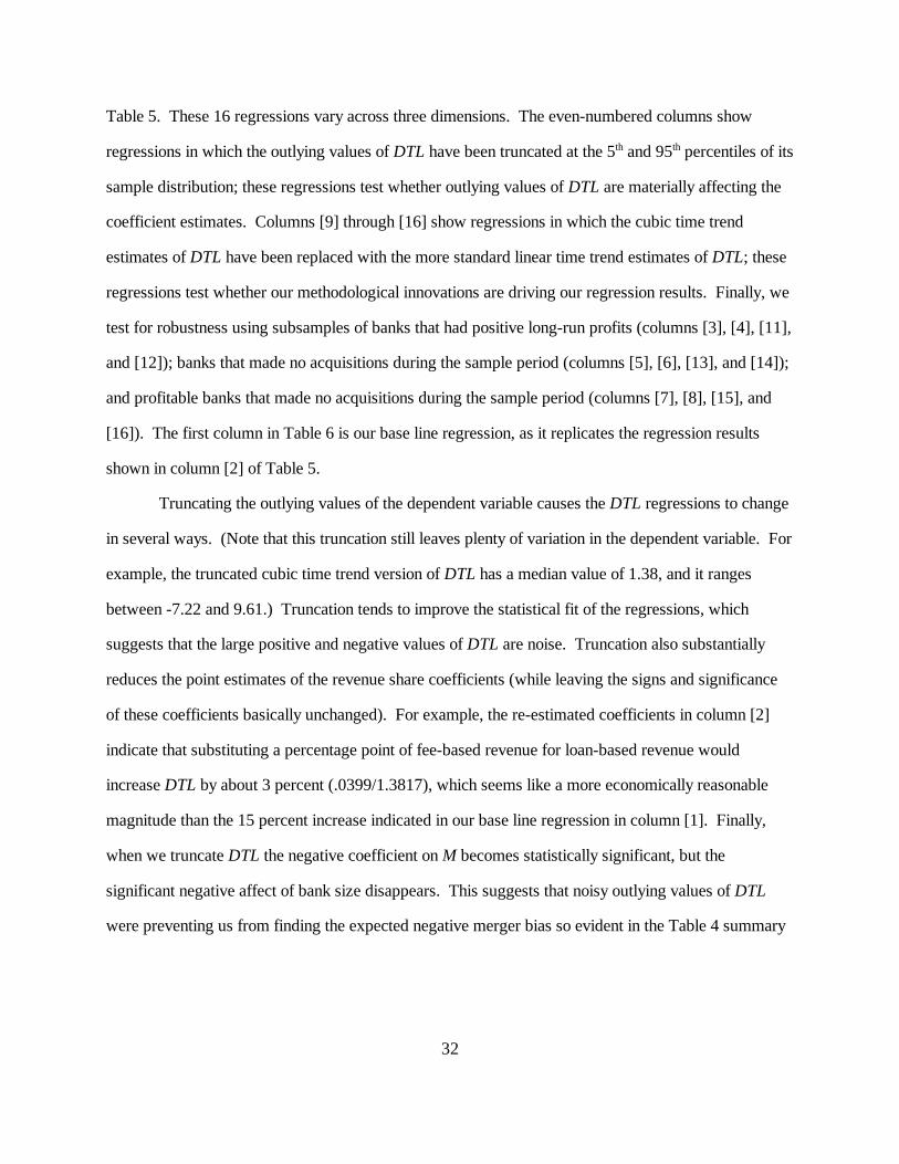
32
Table 5. These 16 regressions vary across three dimensions. The even-numbered columns show
regressions in which the outlying values of DTL have been truncated at the 5 and 95 percentiles of itsth th
sample distribution; these regressions test whether outlying values of DTL are materially affecting the
coefficient estimates. Columns [9] through [16] show regressions in which the cubic time trend
estimates of DTL have been replaced with the more standard linear time trend estimates of DTL; these
regressions test whether our methodological innovations are driving our regression results. Finally, we
test for robustness using subsamples of banks that had positive long-run profits (columns [3], [4], [11],
and [12]); banks that made no acquisitions during the sample period (columns [5], [6], [13], and [14]);
and profitable banks that made no acquisitions during the sample period (columns [7], [8], [15], and
[16]). The first column in Table 6 is our base line regression, as it replicates the regression results
shown in column [2] of Table 5.
Truncating the outlying values of the dependent variable causes the DTL regressions to change
in several ways. (Note that this truncation still leaves plenty of variation in the dependent variable. For
example, the truncated cubic time trend version of DTL has a median value of 1.38, and it ranges
between -7.22 and 9.61.) Truncation tends to improve the statistical fit of the regressions, which
suggests that the large positive and negative values of DTL are noise. Truncation also substantially
reduces the point estimates of the revenue share coefficients (while leaving the signs and significance
of these coefficients basically unchanged). For example, the re-estimated coefficients in column [2]
indicate that substituting a percentage point of fee-based revenue for loan-based revenue would
increase DTL by about 3 percent (.0399/1.3817), which seems like a more economically reasonable
magnitude than the 15 percent increase indicated in our base line regression in column [1]. Finally,
when we truncate DTL the negative coefficient on M becomes statistically significant, but the
significant negative affect of bank size disappears. This suggests that noisy outlying values of DTL
were preventing us from finding the expected negative merger bias so evident in the Table 4 summary
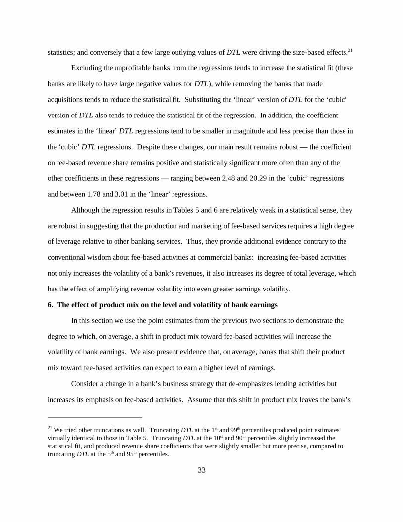
We tried other truncations as well. Truncating DTL at the 1 and 99 percentiles produced point estimates21 st th
virtually identical to those in Table 5. Truncating DTL at the 10 and 90 percentiles slightly increased thest th
statistical fit, and produced revenue share coefficients that were slightly smaller but more precise, compared totruncating DTL at the 5 and 95 percentiles. th th
33
statistics; and conversely that a few large outlying values of DTL were driving the size-based effects.21
Excluding the unprofitable banks from the regressions tends to increase the statistical fit (these
banks are likely to have large negative values for DTL), while removing the banks that made
acquisitions tends to reduce the statistical fit. Substituting the ‘linear’ version of DTL for the ‘cubic’
version of DTL also tends to reduce the statistical fit of the regression. In addition, the coefficient
estimates in the ‘linear’ DTL regressions tend to be smaller in magnitude and less precise than those in
the ‘cubic’ DTL regressions. Despite these changes, our main result remains robust — the coefficient
on fee-based revenue share remains positive and statistically significant more often than any of the
other coefficients in these regressions — ranging between 2.48 and 20.29 in the ‘cubic’ regressions
and between 1.78 and 3.01 in the ‘linear’ regressions.
Although the regression results in Tables 5 and 6 are relatively weak in a statistical sense, they
are robust in suggesting that the production and marketing of fee-based services requires a high degree
of leverage relative to other banking services. Thus, they provide additional evidence contrary to the
conventional wisdom about fee-based activities at commercial banks: increasing fee-based activities
not only increases the volatility of a bank’s revenues, it also increases its degree of total leverage, which
has the effect of amplifying revenue volatility into even greater earnings volatility.
6. The effect of product mix on the level and volatility of bank earnings
In this section we use the point estimates from the previous two sections to demonstrate the
degree to which, on average, a shift in product mix toward fee-based activities will increase the
volatility of bank earnings. We also present evidence that, on average, banks that shift their product
mix toward fee-based activities can expect to earn a higher level of earnings.
Consider a change in a bank’s business strategy that de-emphasizes lending activities but
increases its emphasis on fee-based activities. Assume that this shift in product mix leaves the bank’s
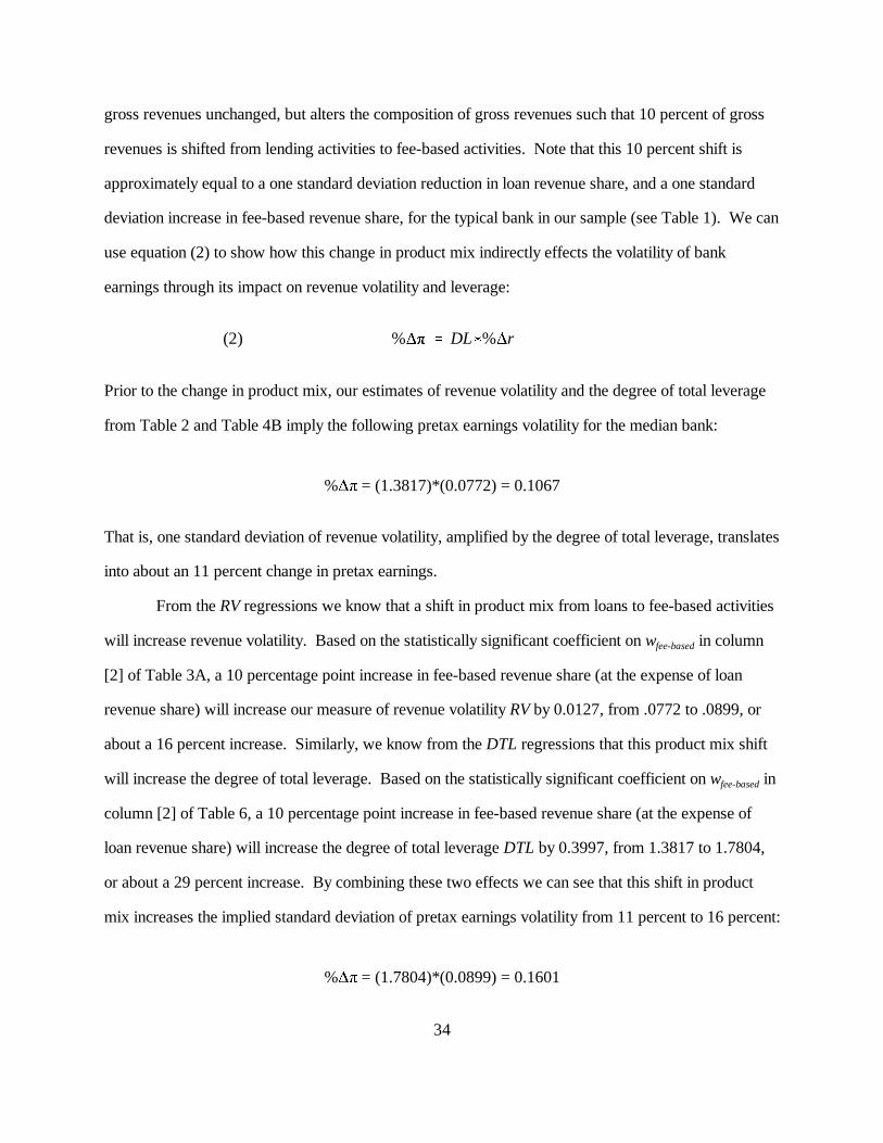
(2) % ' DL(% r
34
gross revenues unchanged, but alters the composition of gross revenues such that 10 percent of gross
revenues is shifted from lending activities to fee-based activities. Note that this 10 percent shift is
approximately equal to a one standard deviation reduction in loan revenue share, and a one standard
deviation increase in fee-based revenue share, for the typical bank in our sample (see Table 1). We can
use equation (2) to show how this change in product mix indirectly effects the volatility of bank
earnings through its impact on revenue volatility and leverage:
Prior to the change in product mix, our estimates of revenue volatility and the degree of total leverage
from Table 2 and Table 4B imply the following pretax earnings volatility for the median bank:
% = (1.3817)*(0.0772) = 0.1067
That is, one standard deviation of revenue volatility, amplified by the degree of total leverage, translates
into about an 11 percent change in pretax earnings.
From the RV regressions we know that a shift in product mix from loans to fee-based activities
will increase revenue volatility. Based on the statistically significant coefficient on w in columnfee-based
[2] of Table 3A, a 10 percentage point increase in fee-based revenue share (at the expense of loan
revenue share) will increase our measure of revenue volatility RV by 0.0127, from .0772 to .0899, or
about a 16 percent increase. Similarly, we know from the DTL regressions that this product mix shift
will increase the degree of total leverage. Based on the statistically significant coefficient on w infee-based
column [2] of Table 6, a 10 percentage point increase in fee-based revenue share (at the expense of
loan revenue share) will increase the degree of total leverage DTL by 0.3997, from 1.3817 to 1.7804,
or about a 29 percent increase. By combining these two effects we can see that this shift in product
mix increases the implied standard deviation of pretax earnings volatility from 11 percent to 16 percent:
% = (1.7804)*(0.0899) = 0.1601
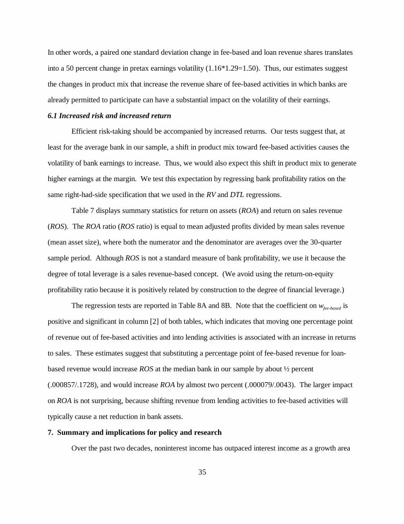
35
In other words, a paired one standard deviation change in fee-based and loan revenue shares translates
into a 50 percent change in pretax earnings volatility (1.16*1.29=1.50). Thus, our estimates suggest
the changes in product mix that increase the revenue share of fee-based activities in which banks are
already permitted to participate can have a substantial impact on the volatility of their earnings.
6.1 Increased risk and increased return
Efficient risk-taking should be accompanied by increased returns. Our tests suggest that, at
least for the average bank in our sample, a shift in product mix toward fee-based activities causes the
volatility of bank earnings to increase. Thus, we would also expect this shift in product mix to generate
higher earnings at the margin. We test this expectation by regressing bank profitability ratios on the
same right-had-side specification that we used in the RV and DTL regressions.
Table 7 displays summary statistics for return on assets (ROA) and return on sales revenue
(ROS). The ROA ratio (ROS ratio) is equal to mean adjusted profits divided by mean sales revenue
(mean asset size), where both the numerator and the denominator are averages over the 30-quarter
sample period. Although ROS is not a standard measure of bank profitability, we use it because the
degree of total leverage is a sales revenue-based concept. (We avoid using the return-on-equity
profitability ratio because it is positively related by construction to the degree of financial leverage.)
The regression tests are reported in Table 8A and 8B. Note that the coefficient on w isfee-based
positive and significant in column [2] of both tables, which indicates that moving one percentage point
of revenue out of fee-based activities and into lending activities is associated with an increase in returns
to sales. These estimates suggest that substituting a percentage point of fee-based revenue for loan-
based revenue would increase ROS at the median bank in our sample by about ½ percent
(.000857/.1728), and would increase ROA by almost two percent (.000079/.0043). The larger impact
on ROA is not surprising, because shifting revenue from lending activities to fee-based activities will
typically cause a net reduction in bank assets.
7. Summary and implications for policy and research
Over the past two decades, noninterest income has outpaced interest income as a growth area
36
for commercial banks. The conventional wisdom among bankers, bank analysts, and bank regulators is
that, because noninterest income is more stable than interest income, this long-run change in bank
product mix has reduced the volatility of bank earnings. To the extent that this is true, the typical
commercial bank should be better able to weather economic downturns today than it was a decade ago.
Taking this logic one step further, expanding commercial bank powers into fee-generating areas such
as insurance and securities brokerage could further reduce the risk of bank failure.
We find evidence that contradicts this conventional wisdom. We analyze the quarterly
movements in revenues and profits at 472 large and medium sized banks between 1988 and 1995,
using a theoretical ‘degree of total leverage’ framework that is not typically applied to financial
institutions. In this framework, the volatility of a bank’s earnings stream is determined by two
independent components: the bank’s revenue volatility, which is determined largely by forces
exogenous to the bank, and the bank’s combined degree of operating and financial leverage, which
reflects production and financing conditions inside the bank. When we apply this theoretical
framework to our data set, we find that both components of earnings volatility increase with the share
of revenues generated by fee-based activities. More specifically, when the median bank in our sample
reduces its interest revenue from traditional originate-and-hold lending activities, and replaces it by
increasing its noninterest income from (perhaps credit-related) fee-for-service activities, the bank’s
earnings are likely to become more volatile. This occurs for two reasons: the bank’s stream of
revenues becomes less stable, and the bank takes on a higher degree of total leverage, which amplifies
the revenue instability. We also find that this shift in product mix from lending activities to fee-based
activities is accompanied by an increase in profitability, at least partially compensating banks for the
increase in volatility.
Although these results are unorthodox, they follow naturally from the different demand and
production characteristics of these two types of banking products. Traditional bank lending is a
relationship business — it is costly for borrowers and/or lenders to walk away from lending
relationships because of switching costs and information costs — so revenues from lending business
37
are likely to be stable over time. Once the lending relationship is established and the fixed costs of
credit evaluation have been incurred, the ongoing production costs are mostly variable (interest) costs,
which reduces operating leverage. Furthermore, the bank must hold some equity capital against
outstanding loan balances, which reduces financial leverage. In contrast, bank-customer relationships
are likely to be less stable in many fee-based activities (e.g., investment advice, mutual fund and
insurance sales, data processing) in which information costs are low and competitive rivalry is high,
and the degree of leverage associated with these activities may be large due to relatively high fixed-to-
variable operating cost ratios and relatively low (or zero) regulatory capital requirements.
Although our main results are unorthodox, we find very plausible and orthodox results for
banks’ non-fee-based activities. For example, we find that an increased reliance on trading activities
increases the volatility of overall bank revenues, and that increased reliance on charging fees to
depositors reduces the volatility of overall bank revenues. We also find that increased reliance on
lending activities and investment activities — both intermediation-based activities which should have
similar production processes and similar sensitivities to changes in interest rates — have statistically
similar impacts on bank revenue volatility and on banks’ degree of total bank leverage. These plausible
results increase the confidence that we have in our innovative empirical framework and in the
unorthodox fee-based results that this framework generates.
7.1 Implications of our results
Our results have implications for regulatory policy, business strategy, and future research
studies. Our main result suggests that increased reliance on fee-based activities can, at least under
some circumstances, make bank earnings more volatile. While diversified investors can neutralize
much of this risk in their portfolios, bank depositors (and the insurance fund) bear a portion of this risk,
particularly at larger banks. Should our results prove to be robust to future testing, bank regulators
may want to consider the appropriate role of capital requirements for fee-based activities. We do not
believe, however, that our results should be used to comment on the current debate over expanded
powers for banks. The activities at the heart of the expanded powers debate (securities brokerage and

Black and Scholes (1973) point out that, for levered firms like banks, higher earnings volatility enhances equity22
value because it increases the probability of a positive payout to shareholders. (This is similar to higher share pricevolatility increasing the probability that the price of the associated call option exceeds its strike price.) Marcus(1984) developed a theoretical model showing that banks are more likely to adopt high-risk strategies when thevalue of their charter is low. Keeley (1990) generated empirical evidence that increases in competition areassociated with reductions in bank charter values, and that reduced charter values are associated with increases inbank default risk due to higher levels of asset risk and financial leverage.
38
insurance activities) are primarily fee-based activities, but the demand and production characteristics of
these activities may differ from those of the fee-based activities included in this study. Furthermore, to
the extent that banking firms participated in these activities during the time period encompassed by our
study, some of these activities would have been located in nonbank holding company affiliates, not in
the banking affiliate. The degree to which our results are useful in this policy debate ultimately
depends on the degree of similarity between the characteristics of the currently permissible fee-based
activities and the proposed expanded powers.
Our results are at odds with the numerous public pronouncements (see the Introduction to this
paper for examples) by banks and bank regulators that expansion into fee-based activities banks
stabilizes bank earnings streams. If fee-based activities do not stabilize earnings, then why have banks
increased these activities relative to their more traditional lines of business? One plausible explanation
is that the value of bank charters fell in the 1980s and 1990s as banks lost market share in their core
products (loans and deposits) due to technological change and increased competition, and with less
charter value at risk, banks sought out ways to increase the volatility of their earnings. This explanation
is rooted in the concept of equity as a call option on the value of the firm’s assets, and is consistent with
research on financial institutions by Marcus (1984) and Keeley (1990). Importantly, this explanation22
also fits the facts at hand. During our sample period, banks faced increased competition from nonbank
financial institutions, and responded by shifting into highly levered product lines (i.e., fee-based
activities) that generated relatively volatile earning streams.
We generate these earnings volatility results using a ‘degree of total leverage’ approach not
generally applied to banking firms. This approach allows us to measure the marginal contribution to
39
earnings volatility of products and services that are already being produced by banks, and thus our
estimates reflect the effects of production synergies (economies of scope), marketing synergies (cross-
selling), and portfolio synergies (diversification effects). This approach also allows us to roughly
decompose earnings volatility into demand-side (revenue volatility) and supply-side (operating and
financial leverage) sources. We encourage other researchers to test this approach for robustness, to
expand upon it, and to improve it.
In addition, we make a number of modifications to the standard leverage estimation
framework. While we designed these modifications with the operational, financial, and strategic
characteristics of commercial banks in mind, our modified approach could also be useful in the
estimation of the degree of total leverage for non-financial firms. Unlike the standard methodology, our
estimation framework accepts firms that are economically viable in the long-run but that suffer negative
profits in the short-run. Also, our non-linear adjustment for growth might be useful for estimating the
degree of leverage at firms in the early growth phase of their industry or product life cycles (e.g., high
technology firms during the 1980s and 1990s). We encourage others to test these modifications for
robustness on nonfinancial firm data.
40
References
Allen, Linda, and Julapa Jagtiani, 1999, “The Impact of Securities and Insurance UnderwritingActivities on Bank Risks,” Federal Reserve Bank of Chicago, unpublished manuscript.
Ahmed, Anwer S., Carolyn Takeda, and Shawn Thomas, 1998, “Bank Loan Loss Provisions: AReexamination of Capital Management, Earnings Management, and Signaling Effects,” SyracuseUniversity, unpublished manuscript.
Barefield, Russell M. and Eugene E. Comiskey, 1979, "The Differential Association of Forecast Errorand Earnings Variability with Systematic Risk," Journal of Business Finance & Accounting 1: 1-8.
Berger, Allen N., and David B. Humphrey, 1992, "Measurement and Efficiency Issues in CommercialBanking," in Z. Griliches, ed., Output Measurement in the Service Sectors, National Bureau ofEconomic Research, Studies in Income and Wealth, Vol. 56, University of Chicago Press (Chicago,IL): 245-79.
Berger, Allen N., Anil Kashyap, and Joseph Scalise, 1995, "The Transformation of the U.S. BankingIndustry: What a Long, Strange Trip It's Been," Brookings Papers on Economic Activity 2: 55-218.
Black, Fisher and Myron Scholes, 1973, “The Pricing of Options and Corporate Liabilities,” Journal ofPolitical Economy 81: 637-654.
Boyd, John H., and Mark Gertler, 1994, "Are Banks Dead? Or are the Reports Greatly Exaggerated?"Federal Reserve Bank of Chicago, Conference on Bank Structure and Regulation, The Declining Roleof Banking, May: 85-117.
Boyd, John H., and Stanley L. Graham , 1986, "Risk, Regulation, and Bank Holding CompanyExpansion into Nonbanking,” Federal Reserve Bank of Minneapolis, Quarterly Review, Spring: 2-17.
Boyd, John H., and Stanley L. Graham, 1991, "Investigating the Banking Consolidation Trend,"Federal Reserve Bank of Minneapolis, Quarterly Review, Spring: 3-15.
Boyd, John H., Stanley L. Graham, and R. Shan Hewitt, 1993, “Bank Holding Company Mergers withNonbank Financial Firms,” Journal of Banking and Finance 17: 43-63.
Boyd, John H., Gerald A. Hanweck, and Pipat Pithyachariyakul, 1980, “Bank Holding CompanyDiversification,” Federal Reserve Bank of Chicago, Proceedings from a Conference on BankStructure and Regulation, May: 105-120.
Demsetz, Rebecca S., and Philip E. Strahan, 1995, “Diversification, Size and Risk at Bank HoldingCompanies,” Federal Reserve bank of New York, Research Paper #9506.
41
DeYoung, Robert, 1994, "Fee-Based Services and Cost Efficiency in Commercial Banks," FederalReserve Bank of Chicago, Proceedings from a Conference on Bank Structure and Regulation, May:501-519.
DeYoung, Robert, and Karin P. Roland, 1997, “Commercial Bank Product Mix, Leverage, andEarnings,” unpublished manuscript, presented at the Atlantic Economic Society meetings, Philadelphia.
Dugan, Michael T., and Keith A. Shriver, 1992, “The Effects of Estimation Period, Industry, andProxy on the Calculation of the Degree of Operating Leverage,” The Financial Review 24: 309-321.
Edwards, Franklin R., and Frederic S. Mishkin, 1995, “The Decline of Traditional Banking:Implications for Financial Stability and Regulatory Policy,” Federal Reserve Bank of New York,Economic Policy Review July: 27-45.
Eisenbeis, Robert A., Robert S. Harris, and Josef Lakonishok, 1984, “Benefits of Bank Diversification:The Evidence from Shareholder Returns,” Journal of Finance 39: 881-890.
Gallo, John G., Vincent P. Apilado, and James W. Kolari, 1996, “Commercial Bank Mutual FundActivities: Implications for Bank Risk and Profitability,” Journal of Banking and Finance 20: 1775-1791.
Heggestad, Arnold, 1975, “Riskiness of Investments in Nonbank Activities by Bank HoldingCompanies,” Journal of Economics and Business, 219-223.
Humphrey, David, B., 1990, "Why Do Estimates of Bank Scale Economies Differ?," Federal ReserveBank of Richmond, Economic Review, September: 38-50.
Johnson, Rodney D., and David R. Meinster, 1974, “Bank Holding Companies: DiversificationOpportunities in Nonbank Activities,” Eastern Economic Journal, 316-323.
Kaufman, George G., and Larry R. Mote, 1994, "Is Banking a Declining Industry? An HistoricalPerspective," Economic Perspectives, Federal Reserve Bank of Chicago, May/June: 2-21.
Keeley, Michael C., 1990, “Deposit Insurance, Risk, and Market Power in Banking,” AmericanEconomic Review 80: 1183-1200.
Kwan, Simon H., 1998, “Securities Activities by Commercial Banking Firms’ Section 20 Subsidiaries:Risk, Return, and Diversification Benefits,” Federal Reserve Bank of Chicago, Proceedings from aConference on Bank Structure and Regulation, May: 531-552.
Kwast, Myron L., 1989, “The Impact of Underwriting and Dealing on Bank Returns and Risks,”Journal of Banking and Finance 13: 101-125.
Laderman, Elizabeth S., 1998, “The Potential Diversification and Failure Reduction Benefits of BankExpansion into Nonbanking Activities,” manuscript, Federal Reserve Bank of San Francisco.
42
Litan, Robert E., 1985, “Evaluating and Controlling the Risks of Financial Product Deregulation,” YaleJournal of Regulation 3: 1-52.
Litzenberger, Robert H. and Cherukuri U. Rao, 1971, "Estimates of the Marginal Rate of TimePreference and Average Risk Aversion of Investors in Electric Utility Shares: 1960-66," The BellJournal of Economics and Management Science, Spring: 365-377.
Lord, Richard A., 1998, “Properties of Time Series Estimates of Degree of Leverage Measures,” TheFinancial Review 33: 69-84.
Mandelker, G. and S.G. Rhee, 1984, “The Impact of the Degree of Operating and Financial Leverageon Systematic Risk of Common Stock,” Journal of Financial and Quantitative Analysis 19: 45-57.
Marcus, Alan J., 1984, “Deregulation and Bank Financial Policy,” Journal of Banking and Finance 8:557-565.
O’Brien, T., and P. Vanderheiden, 1987, “Empirical Measurement of Operating Leverage for GrowingFirms,” Financial Management 16: 45-53.
Roland, Karin P., 1997, “Profit Persistence in Large U.S. Bank Holding Companies: An EmpiricialInvestigation,” Office of the Comptroller of the Currency, Economics Working Paper 97-2.
Sinkey, Jr., Joseph F., and Robert C. Nash, 1993, “Assessing the Riskiness and Profitability of Credit-Card Banks,” Journal of Financial Services Research 7: 127-150.
Spong, Kenneth, 1994, Banking Regulation: Its Purposes, Implementation, and Effects, 4th edition,Kansas City: Federal Reserve Bank of Kansas City.
Tripplet, Jack E., 1992, "Banking Output," The New Palgrave Dictionary of Money and Finance, ed.Peter Newman, Murray Milgate, and John Eatwell, London: MacMillin Press, 143-146.
Wall, Larry D., and Robert A. Eisenbeis, 1984, “Risk Considerations in Deregulating Bank Activities,”Federal Reserve Bank of Atlanta, Economic Review, May, 6-19.
Wall, Larry D., Alan K. Reichert, and Sunil Mohanty, 1993, “Deregulation and the Opportunities forCommercial Bank Diversification,” Federal Reserve Bank of Atlanta, Economic Review,September/October, 1-25.
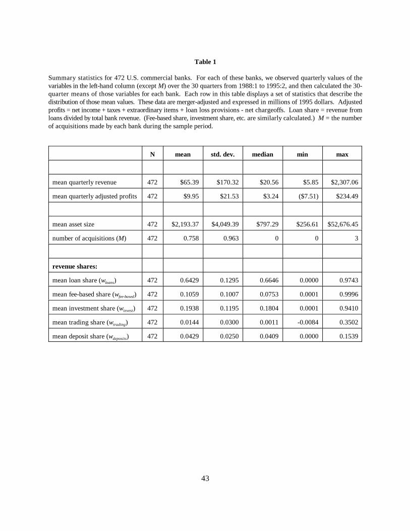
43
Table 1
Summary statistics for 472 U.S. commercial banks. For each of these banks, we observed quarterly values of thevariables in the left-hand column (except M) over the 30 quarters from 1988:1 to 1995:2, and then calculated the 30-quarter means of those variables for each bank. Each row in this table displays a set of statistics that describe thedistribution of those mean values. These data are merger-adjusted and expressed in millions of 1995 dollars. Adjustedprofits = net income + taxes + extraordinary items + loan loss provisions - net chargeoffs. Loan share = revenue fromloans divided by total bank revenue. (Fee-based share, investment share, etc. are similarly calculated.) M = the numberof acquisitions made by each bank during the sample period.
N mean std. dev. median min max
mean quarterly revenue 472 $65.39 $170.32 $20.56 $5.85 $2,307.06
mean quarterly adjusted profits 472 $9.95 $21.53 $3.24 ($7.51) $234.49
mean asset size 472 $2,193.37 $4,049.39 $797.29 $256.61 $52,676.45
number of acquisitions (M) 472 0.758 0.963 0 0 3
revenue shares:
mean loan share (w ) 472 0.6429 0.1295 0.6646 0.0000 0.9743loans
mean fee-based share (w ) 472 0.1059 0.1007 0.0753 0.0001 0.9996fee-based
mean investment share (w ) 472 0.1938 0.1195 0.1804 0.0001 0.9410invest
mean trading share (w ) 472 0.0144 0.0300 0.0011 -0.0084 0.3502trading
mean deposit share (w ) 472 0.0429 0.0250 0.0409 0.0000 0.1539deposits
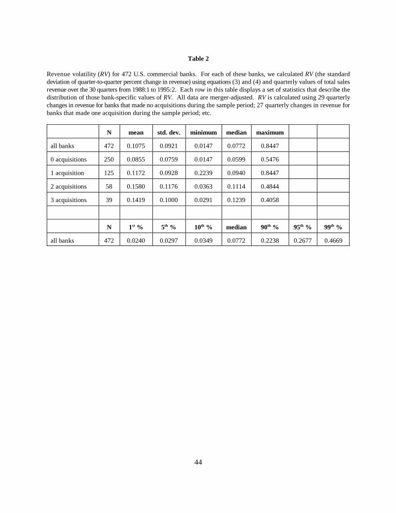
44
Table 2
Revenue volatility (RV) for 472 U.S. commercial banks. For each of these banks, we calculated RV (the standarddeviation of quarter-to-quarter percent change in revenue) using equations (3) and (4) and quarterly values of total salesrevenue over the 30 quarters from 1988:1 to 1995:2. Each row in this table displays a set of statistics that describe thedistribution of those bank-specific values of RV. All data are merger-adjusted. RV is calculated using 29 quarterlychanges in revenue for banks that made no acquisitions during the sample period; 27 quarterly changes in revenue forbanks that made one acquisition during the sample period; etc.
N mean std. dev. minimum median maximum
all banks 472 0.1075 0.0921 0.0147 0.0772 0.8447
0 acquisitions 250 0.0855 0.0759 0.0147 0.0599 0.5476
1 acquisition 125 0.1172 0.0928 0.2239 0.0940 0.8447
2 acquisitions 58 0.1580 0.1176 0.0363 0.1114 0.4844
3 acquisitions 39 0.1419 0.1000 0.0291 0.1239 0.4058
N 1 % 5 % 10 % median 90 % 95 % 99 %st th th th th th
all banks 472 0.0240 0.0297 0.0349 0.0772 0.2238 0.2677 0.4669
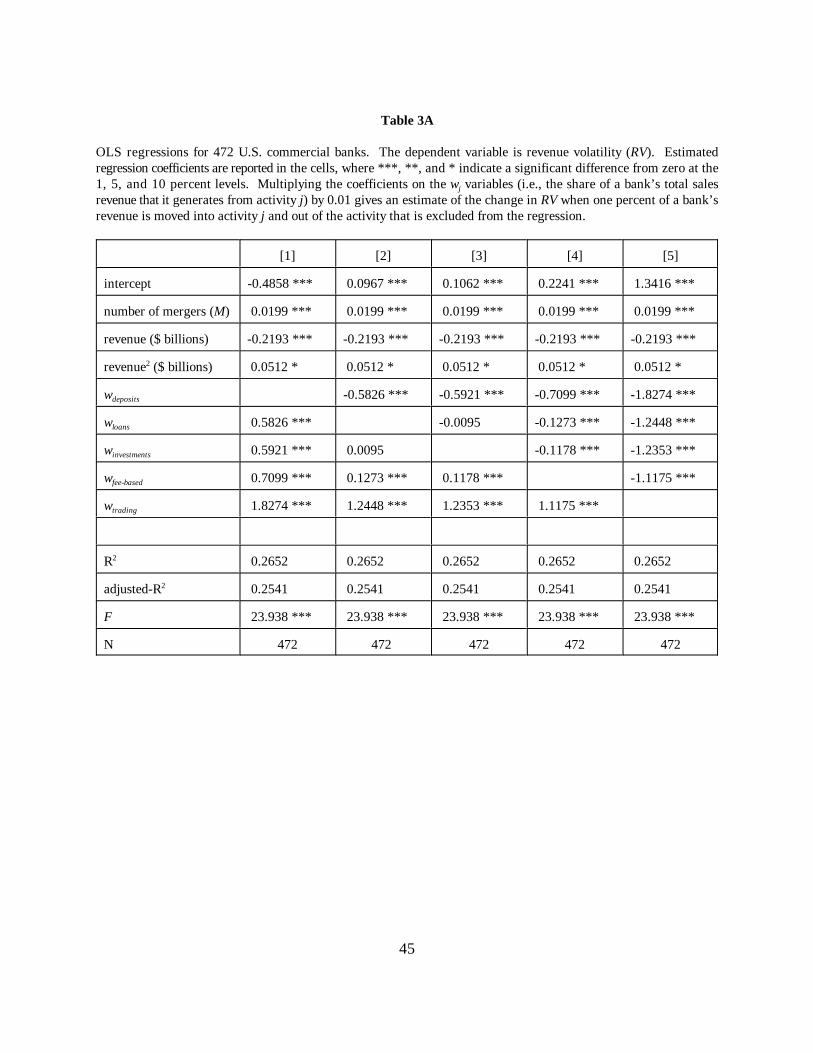
45
Table 3A
OLS regressions for 472 U.S. commercial banks. The dependent variable is revenue volatility (RV). Estimatedregression coefficients are reported in the cells, where ***, **, and * indicate a significant difference from zero at the1, 5, and 10 percent levels. Multiplying the coefficients on the w variables (i.e., the share of a bank’s total salesj
revenue that it generates from activity j) by 0.01 gives an estimate of the change in RV when one percent of a bank’srevenue is moved into activity j and out of the activity that is excluded from the regression.
[1] [2] [3] [4] [5]
intercept -0.4858 *** 0.0967 *** 0.1062 *** 0.2241 *** 1.3416 ***
number of mergers (M) 0.0199 *** 0.0199 *** 0.0199 *** 0.0199 *** 0.0199 ***
revenue ($ billions) -0.2193 *** -0.2193 *** -0.2193 *** -0.2193 *** -0.2193 ***
revenue ($ billions) 0.0512 * 0.0512 * 0.0512 * 0.0512 * 0.0512 *2
w -0.5826 *** -0.5921 *** -0.7099 *** -1.8274 ***deposits
w 0.5826 *** -0.0095 -0.1273 *** -1.2448 ***loans
w 0.5921 *** 0.0095 -0.1178 *** -1.2353 ***investments
w 0.7099 *** 0.1273 *** 0.1178 *** -1.1175 ***fee-based
w 1.8274 *** 1.2448 *** 1.2353 *** 1.1175 ***trading
R 0.2652 0.2652 0.2652 0.2652 0.26522
adjusted-R 0.2541 0.2541 0.2541 0.2541 0.25412
F 23.938 *** 23.938 *** 23.938 *** 23.938 *** 23.938 ***
N 472 472 472 472 472
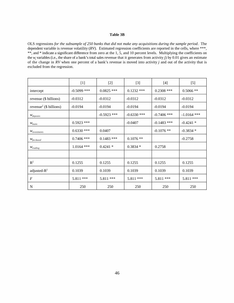
46
Table 3B
OLS regressions for the subsample of 250 banks that did not make any acquisitions during the sample period. Thedependent variable is revenue volatility (RV). Estimated regression coefficients are reported in the cells, where ***,**, and * indicate a significant difference from zero at the 1, 5, and 10 percent levels. Multiplying the coefficients onthe w variables (i.e., the share of a bank’s total sales revenue that it generates from activity j) by 0.01 gives an estimatej
of the change in RV when one percent of a bank’s revenue is moved into activity j and out of the activity that isexcluded from the regression.
[1] [2] [3] [4] [5]
intercept -0.5099 *** 0.0825 *** 0.1232 *** 0.2308 *** 0.5066 **
revenue ($ billions) -0.0312 -0.0312 -0.0312 -0.0312 -0.0312
revenue ($ billions) -0.0194 -0.0194 -0.0194 -0.0194 -0.01942
w -0.5923 *** -0.6330 *** -0.7406 *** -1.0164 ***deposits
w 0.5923 *** -0.0407 -0.1483 *** -0.4241 *loans
w 0.6330 *** 0.0407 -0.1076 ** -0.3834 *investments
w 0.7406 *** 0.1483 *** 0.1076 ** -0.2758 fee-based
w 1.0164 *** 0.4241 * 0.3834 * 0.2758 trading
R 0.1255 0.1255 0.1255 0.1255 0.12552
adjusted-R 0.1039 0.1039 0.1039 0.1039 0.10392
F 5.811 *** 5.811 *** 5.811 *** 5.811 *** 5.811 ***
N 250 250 250 250 250
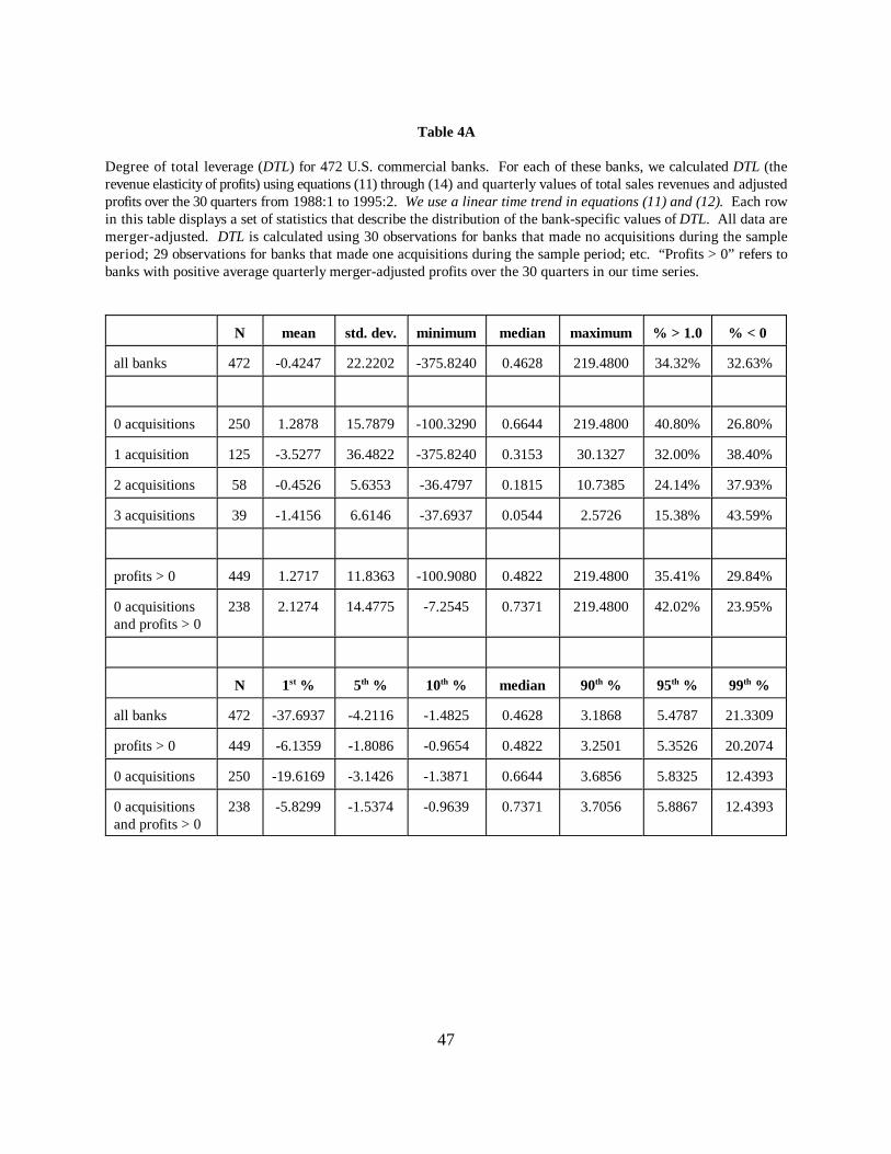
47
Table 4A
Degree of total leverage (DTL) for 472 U.S. commercial banks. For each of these banks, we calculated DTL (therevenue elasticity of profits) using equations (11) through (14) and quarterly values of total sales revenues and adjustedprofits over the 30 quarters from 1988:1 to 1995:2. We use a linear time trend in equations (11) and (12). Each rowin this table displays a set of statistics that describe the distribution of the bank-specific values of DTL. All data aremerger-adjusted. DTL is calculated using 30 observations for banks that made no acquisitions during the sampleperiod; 29 observations for banks that made one acquisitions during the sample period; etc. “Profits > 0” refers tobanks with positive average quarterly merger-adjusted profits over the 30 quarters in our time series.
N mean std. dev. minimum median maximum % > 1.0 % < 0
all banks 472 -0.4247 22.2202 -375.8240 0.4628 219.4800 34.32% 32.63%
0 acquisitions 250 1.2878 15.7879 -100.3290 0.6644 219.4800 40.80% 26.80%
1 acquisition 125 -3.5277 36.4822 -375.8240 0.3153 30.1327 32.00% 38.40%
2 acquisitions 58 -0.4526 5.6353 -36.4797 0.1815 10.7385 24.14% 37.93%
3 acquisitions 39 -1.4156 6.6146 -37.6937 0.0544 2.5726 15.38% 43.59%
profits > 0 449 1.2717 11.8363 -100.9080 0.4822 219.4800 35.41% 29.84%
0 acquisitions 238 2.1274 14.4775 -7.2545 0.7371 219.4800 42.02% 23.95%and profits > 0
N 1 % 5 % 10 % median 90 % 95 % 99 %st th th th th th
all banks 472 -37.6937 -4.2116 -1.4825 0.4628 3.1868 5.4787 21.3309
profits > 0 449 -6.1359 -1.8086 -0.9654 0.4822 3.2501 5.3526 20.2074
0 acquisitions 250 -19.6169 -3.1426 -1.3871 0.6644 3.6856 5.8325 12.4393
0 acquisitions 238 -5.8299 -1.5374 -0.9639 0.7371 3.7056 5.8867 12.4393and profits > 0

48
Table 4B
Degree of total leverage (DTL) for 472 U.S. commercial banks. For each of these banks, we calculated DTL (therevenue elasticity of profits) using equations (11) through (14) and quarterly values of total sales revenues andadjusted profits over the 30 quarters from 1988:1 to 1995:2. We use a cubic time trend in equations (11) and (12). Each row in this table displays a set of statistics that describe the distribution of the bank-specific values of DTL. All data are merger-adjusted. DTL is calculated using 30 observations for banks that made no acquisitions duringthe sample period; 29 observations for banks that made one acquisitions during the sample period; etc. “Profits >0” refers to banks with positive average quarterly merger-adjusted profits over the 30 quarters in our time series.
N mean std. dev. minimum median maximum % > 1.0 % < 0
all banks 472 0.3087 17.2438 -214.4444 1.3817 63.3016 56.36% 25.85%
0 acquisitions 250 1.7674 9.8166 -96.0150 1.8822 60.9262 66.80% 19.60%
1 acquisition 125 -1.9394 29.0429 -214.4444 1.0034 63.3016 50.40% 29.60%
2 acquisitions 58 0.1446 8.5951 -55.2394 0.3825 12.2977 41.38% 36.21%
3 acquisitions 39 -1.5927 12.5079 -68.5510 0.3515 13.4739 30.77% 38.46%
profits > 0 449 2.2037 7.9092 -91.0823 1.4948 63.3016 58.57% 22.72%
0 acquisitions 238 2.9278 6.0295 -8.9404 1.9417 60.9262 69.33% 16.39%and profits > 0
N 1 % 5 % 10 % median 90 % 95 % 99 %st th th th th th
all banks 472 -68.5510 -7.2194 -1.4405 1.3817 5.8018 9.6067 34.4415
profits > 0 449 -8.7275 -1.6796 -0.8653 1.4948 5.8018 9.6067 34.4415
0 acquisitions 250 -26.882 -4.1514 -1.2129 1.8822 6.1275 9.7352 43.1045
0 acquisitions 238 -4.5016 -1.4405 -0.6387 1.9417 6.1242 9.8381 43.1045and profits > 0
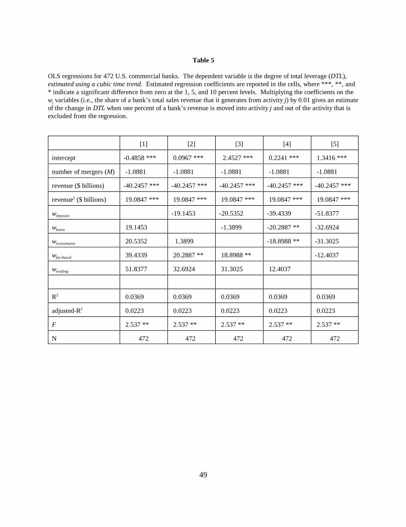
49
Table 5
OLS regressions for 472 U.S. commercial banks. The dependent variable is the degree of total leverage (DTL),estimated using a cubic time trend. Estimated regression coefficients are reported in the cells, where ***, **, and* indicate a significant difference from zero at the 1, 5, and 10 percent levels. Multiplying the coefficients on thew variables (i.e., the share of a bank’s total sales revenue that it generates from activity j) by 0.01 gives an estimatej
of the change in DTL when one percent of a bank’s revenue is moved into activity j and out of the activity that isexcluded from the regression.
[1] [2] [3] [4] [5]
intercept -0.4858 *** 0.0967 *** 2.4527 *** 0.2241 *** 1.3416 ***
number of mergers (M) -1.0881 -1.0881 -1.0881 -1.0881 -1.0881
revenue ($ billions) -40.2457 *** -40.2457 *** -40.2457 *** -40.2457 *** -40.2457 ***
revenue ($ billions) 19.0847 *** 19.0847 *** 19.0847 *** 19.0847 *** 19.0847 ***2
w -19.1453 -20.5352 -39.4339 -51.8377deposits
w 19.1453 -1.3899 -20.2887 ** -32.6924loans
w 20.5352 1.3899 -18.8988 ** -31.3025investments
w 39.4339 20.2887 ** 18.8988 ** -12.4037fee-based
w 51.8377 32.6924 31.3025 12.4037 trading
R 0.0369 0.0369 0.0369 0.0369 0.03692
adjusted-R 0.0223 0.0223 0.0223 0.0223 0.02232
F 2.537 ** 2.537 ** 2.537 ** 2.537 ** 2.537 **
N 472 472 472 472 472
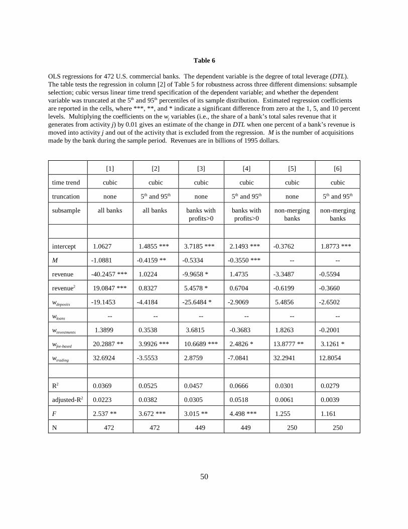
50
Table 6
OLS regressions for 472 U.S. commercial banks. The dependent variable is the degree of total leverage (DTL). The table tests the regression in column [2] of Table 5 for robustness across three different dimensions: subsampleselection; cubic versus linear time trend specification of the dependent variable; and whether the dependentvariable was truncated at the 5 and 95 percentiles of its sample distribution. Estimated regression coefficientsth th
are reported in the cells, where ***, **, and * indicate a significant difference from zero at the 1, 5, and 10 percentlevels. Multiplying the coefficients on the w variables (i.e., the share of a bank’s total sales revenue that itj
generates from activity j) by 0.01 gives an estimate of the change in DTL when one percent of a bank’s revenue ismoved into activity j and out of the activity that is excluded from the regression. M is the number of acquisitionsmade by the bank during the sample period. Revenues are in billions of 1995 dollars.
[1] [2] [3] [4] [5] [6]
time trend cubic cubic cubic cubic cubic cubic
truncation none 5 and 95 none 5 and 95 none 5 and 95th th th th th th
subsample all banks all banks banks with banks with non-merging non-mergingprofits>0 profits>0 banks banks
intercept 1.0627 1.4855 *** 3.7185 *** 2.1493 *** -0.3762 1.8773 ***
M -1.0881 -0.4159 ** -0.5334 -0.3550 *** -- --
revenue -40.2457 *** 1.0224 -9.9658 * 1.4735 -3.3487 -0.5594
revenue 19.0847 *** 0.8327 5.4578 * 0.6704 -0.6199 -0.36602
w -19.1453 -4.4184 -25.6484 * -2.9069 5.4856 -2.6502deposits
w -- -- -- -- -- --loans
w 1.3899 0.3538 3.6815 -0.3683 1.8263 -0.2001 investments
w 20.2887 ** 3.9926 *** 10.6689 *** 2.4826 * 13.8777 ** 3.1261 *fee-based
w 32.6924 -3.5553 2.8759 -7.0841 32.2941 12.8054trading
R 0.0369 0.0525 0.0457 0.0666 0.0301 0.02792
adjusted-R 0.0223 0.0382 0.0305 0.0518 0.0061 0.00392
F 2.537 ** 3.672 *** 3.015 ** 4.498 *** 1.255 1.161
N 472 472 449 449 250 250
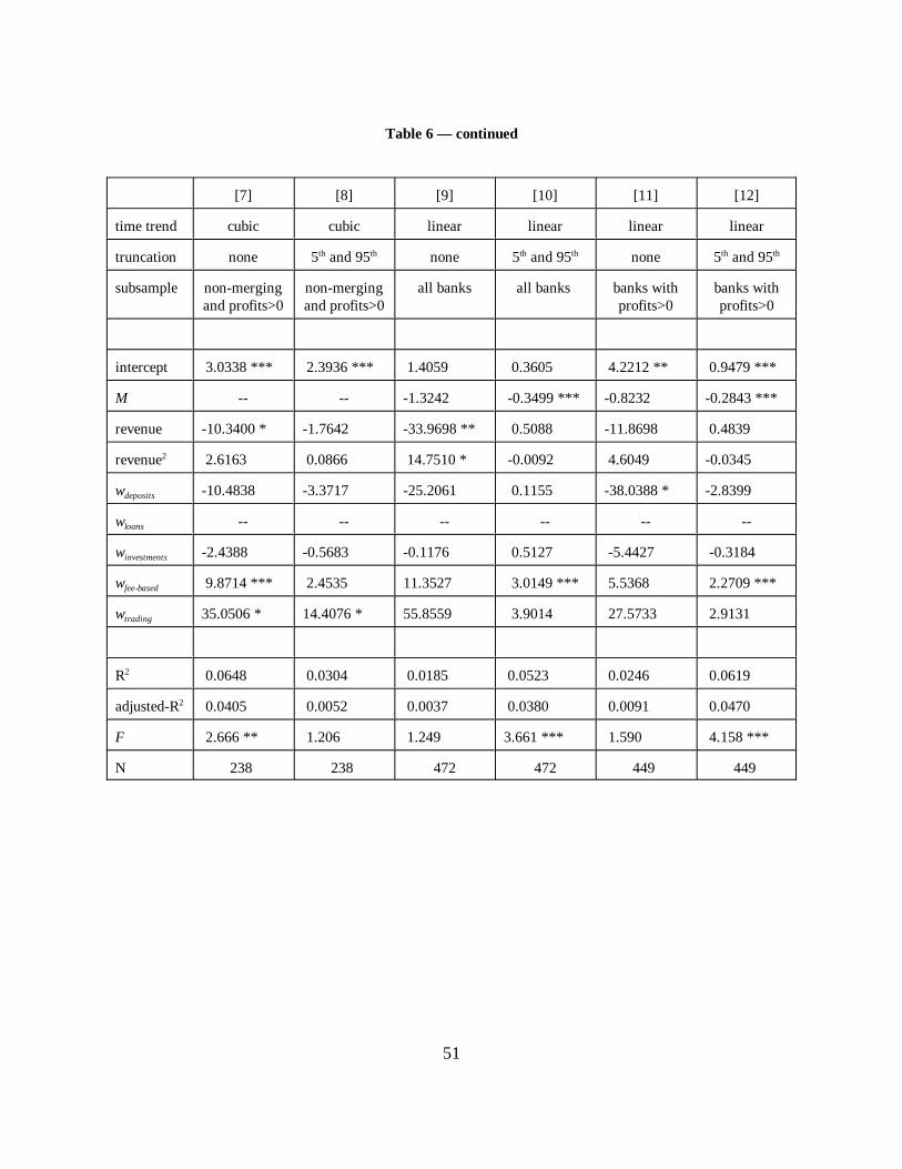
51
Table 6 — continued
[7] [8] [9] [10] [11] [12]
time trend cubic cubic linear linear linear linear
truncation none 5 and 95 none 5 and 95 none 5 and 95th th th th th th
subsample non-merging non-merging all banks all banks banks with banks withand profits>0 and profits>0 profits>0 profits>0
intercept 3.0338 *** 2.3936 *** 1.4059 0.3605 4.2212 ** 0.9479 ***
M -- -- -1.3242 -0.3499 *** -0.8232 -0.2843 ***
revenue -10.3400 * -1.7642 -33.9698 ** 0.5088 -11.8698 0.4839
revenue 2.6163 0.0866 14.7510 * -0.0092 4.6049 -0.03452
w -10.4838 -3.3717 -25.2061 0.1155 -38.0388 * -2.8399deposits
w -- -- -- -- -- --loans
w -2.4388 -0.5683 -0.1176 0.5127 -5.4427 -0.3184investments
w 9.8714 *** 2.4535 11.3527 3.0149 *** 5.5368 2.2709 ***fee-based
w 35.0506 * 14.4076 * 55.8559 3.9014 27.5733 2.9131trading
R 0.0648 0.0304 0.0185 0.0523 0.0246 0.06192
adjusted-R 0.0405 0.0052 0.0037 0.0380 0.0091 0.04702
F 2.666 ** 1.206 1.249 3.661 *** 1.590 4.158 ***
N 238 238 472 472 449 449
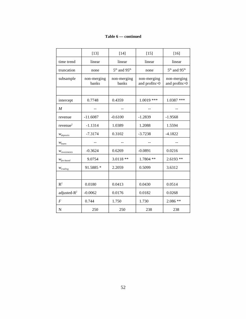
52
Table 6 — continued
[13] [14] [15] [16]
time trend linear linear linear linear
truncation none 5 and 95 none 5 and 95th th th th
subsample non-merging non-merging non-merging non-mergingbanks banks and profits>0 and profits>0
intercept 0.7748 0.4359 1.0019 *** 1.0387 ***
M -- -- -- --
revenue -11.6087 -0.6100 -1.2839 -1.9568
revenue -1.1314 1.0389 1.2088 1.55942
w -7.3174 0.3102 -3.7238 -4.1822deposits
w -- -- -- --loans
w -0.3624 0.6269 -0.0891 0.0216investments
w 9.0754 3.0118 ** 1.7804 ** 2.6193 **fee-based
w 91.5885 * 2.2059 0.5099 3.6312trading
R 0.0180 0.0413 0.0430 0.05142
adjusted-R -0.0062 0.0176 0.0182 0.02682
F 0.744 1.750 1.730 2.086 **
N 250 250 238 238
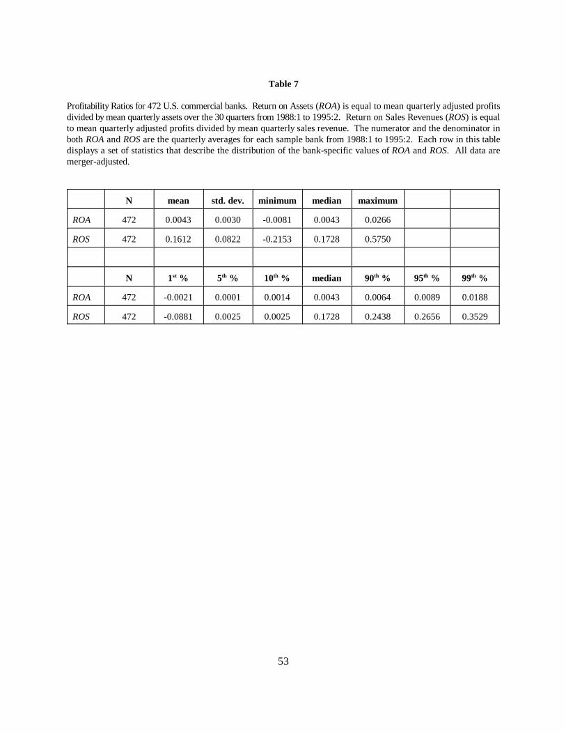
53
Table 7
Profitability Ratios for 472 U.S. commercial banks. Return on Assets (ROA) is equal to mean quarterly adjusted profitsdivided by mean quarterly assets over the 30 quarters from 1988:1 to 1995:2. Return on Sales Revenues (ROS) is equalto mean quarterly adjusted profits divided by mean quarterly sales revenue. The numerator and the denominator inboth ROA and ROS are the quarterly averages for each sample bank from 1988:1 to 1995:2. Each row in this tabledisplays a set of statistics that describe the distribution of the bank-specific values of ROA and ROS. All data aremerger-adjusted.
N mean std. dev. minimum median maximum
ROA 472 0.0043 0.0030 -0.0081 0.0043 0.0266
ROS 472 0.1612 0.0822 -0.2153 0.1728 0.5750
N 1 % 5 % 10 % median 90 % 95 % 99 %st th th th th th
ROA 472 -0.0021 0.0001 0.0014 0.0043 0.0064 0.0089 0.0188
ROS 472 -0.0881 0.0025 0.0025 0.1728 0.2438 0.2656 0.3529
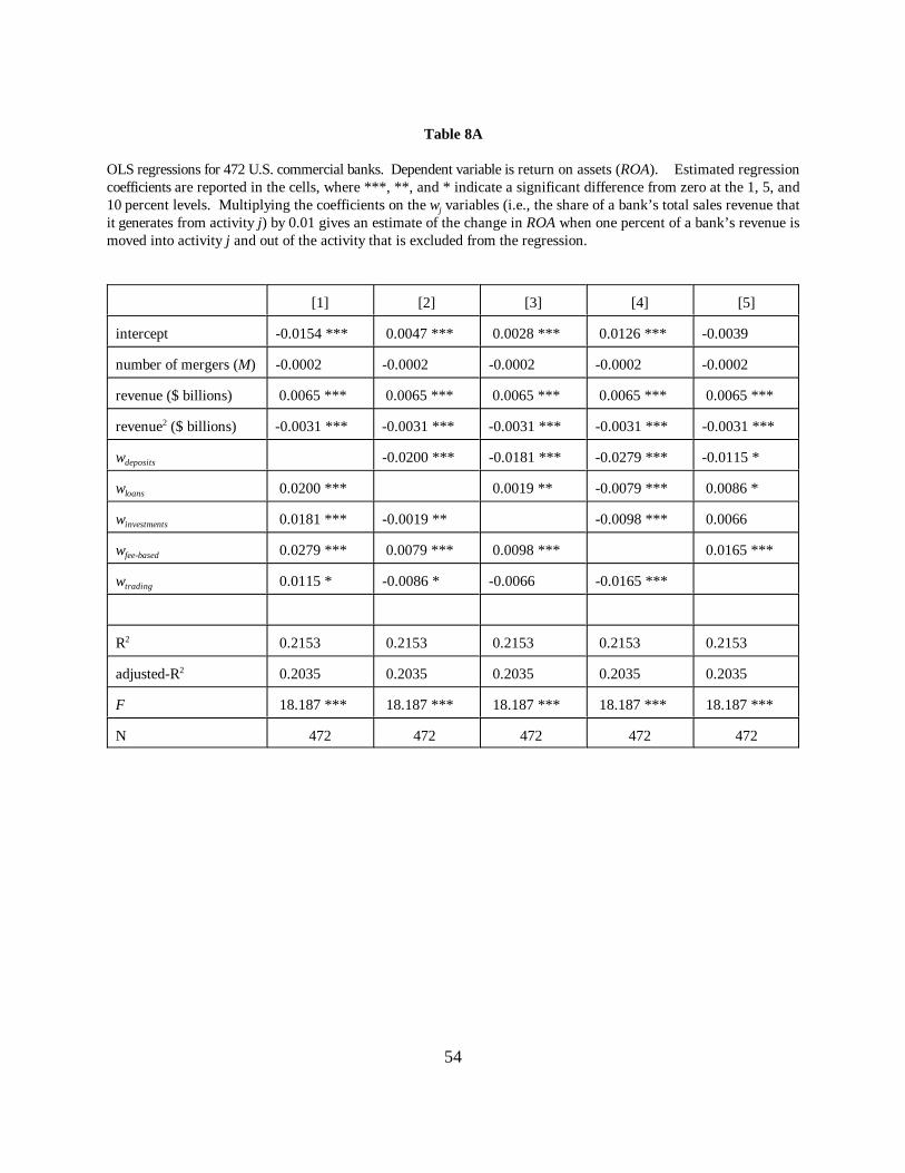
54
Table 8A
OLS regressions for 472 U.S. commercial banks. Dependent variable is return on assets (ROA). Estimated regressioncoefficients are reported in the cells, where ***, **, and * indicate a significant difference from zero at the 1, 5, and10 percent levels. Multiplying the coefficients on the w variables (i.e., the share of a bank’s total sales revenue thatj
it generates from activity j) by 0.01 gives an estimate of the change in ROA when one percent of a bank’s revenue ismoved into activity j and out of the activity that is excluded from the regression.
[1] [2] [3] [4] [5]
intercept -0.0154 *** 0.0047 *** 0.0028 *** 0.0126 *** -0.0039
number of mergers (M) -0.0002 -0.0002 -0.0002 -0.0002 -0.0002
revenue ($ billions) 0.0065 *** 0.0065 *** 0.0065 *** 0.0065 *** 0.0065 ***
revenue ($ billions) -0.0031 *** -0.0031 *** -0.0031 *** -0.0031 *** -0.0031 ***2
w -0.0200 *** -0.0181 *** -0.0279 *** -0.0115 *deposits
w 0.0200 *** 0.0019 ** -0.0079 *** 0.0086 *loans
w 0.0181 *** -0.0019 ** -0.0098 *** 0.0066 investments
w 0.0279 *** 0.0079 *** 0.0098 *** 0.0165 ***fee-based
w 0.0115 * -0.0086 * -0.0066 -0.0165 ***trading
R 0.2153 0.2153 0.2153 0.2153 0.21532
adjusted-R 0.2035 0.2035 0.2035 0.2035 0.20352
F 18.187 *** 18.187 *** 18.187 *** 18.187 *** 18.187 ***
N 472 472 472 472 472
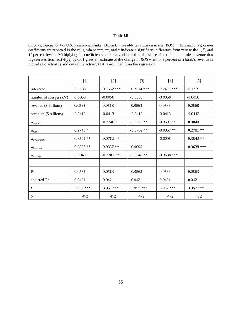
55
Table 8B
OLS regressions for 472 U.S. commercial banks. Dependent variable is return on assets (ROS). Estimated regressioncoefficients are reported in the cells, where ***, **, and * indicate a significant difference from zero at the 1, 5, and10 percent levels. Multiplying the coefficients on the w variables (i.e., the share of a bank’s total sales revenue thatj
it generates from activity j) by 0.01 gives an estimate of the change in ROS when one percent of a bank’s revenue ismoved into activity j and out of the activity that is excluded from the regression.
[1] [2] [3] [4] [5]
intercept -0.1188 0.1552 *** 0.2314 *** 0.2409 *** -0.1229
number of mergers (M) -0.0058 -0.0058 -0.0058 -0.0058 -0.0058
revenue ($ billions) 0.0568 0.0568 0.0568 0.0568 0.0568
revenue ($ billions) -0.0413 -0.0413 -0.0413 -0.0413 -0.04132
w -0.2740 * -0.3502 ** -0.3597 ** 0.0040deposits
w 0.2740 * -0.0762 ** -0.0857 ** 0.2781 **loans
w 0.3502 ** 0.0762 ** -0.0095 0.3542 **investments
w 0.3597 ** 0.0857 ** 0.0095 0.3638 ***fee-based
w -0.0040 -0.2781 ** -0.3542 ** -0.3638 ***trading
R 0.0563 0.0563 0.0563 0.0563 0.05632
adjusted-R 0.0421 0.0421 0.0421 0.0421 0.04212
F 3.957 *** 3.957 *** 3.957 *** 3.957 *** 3.957 ***
N 472 472 472 472 472
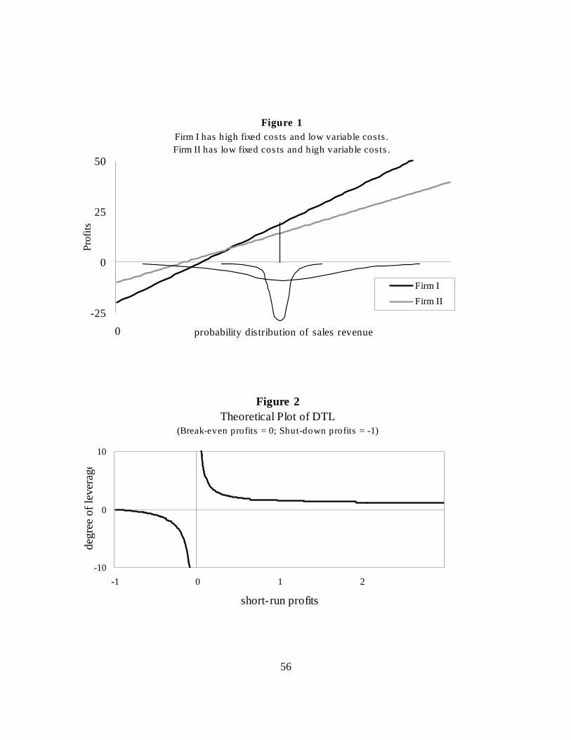
Figure 1Firm I has high fixed cos ts and low variable costs .Firm II has low fixed cos ts and high variable costs .
-25
0
25
50
0 probability distribution of sales revenue
Pro
fits
Firm I
Firm II
Figure 2Theoretical Plot of DTL
(Break-even profits = 0; Shut-down profits = -1)
-10
0
10
-1 0 1 2
short-run profits
degr
ee o
f le
vera
ge
56

Figure 3Mean Revenue by Quarter for 472 Sample Banks
$80,000
$90,000
$100,000
$110,000
$120,000
$130,000
1 5 9 13 17 21 25 29time (quarters)
reve
nue
($th
ousa
nds
Figure 4Mean Profits by Quarter for 472 Sample Banks
$0
$5,000
$10,000
$15,000
$20,000
$25,000
1 5 9 13 17 21 25 29time (quarters)
prof
its (
$tho
usan
ds
57
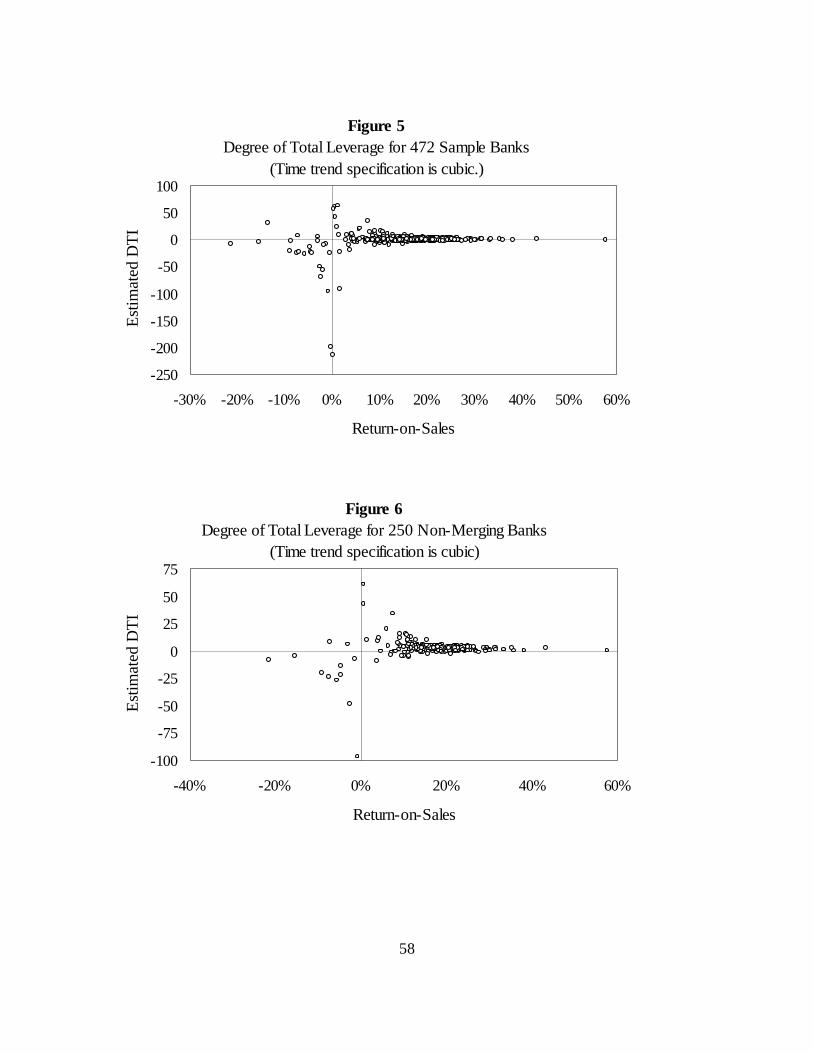
Figure 5Degree of Total Leverage for 472 Sample Banks
(Time trend specification is cubic.)
-250
-200
-150
-100
-50
0
50
100
-30% -20% -10% 0% 10% 20% 30% 40% 50% 60%
Return-on-Sales
Est
imat
ed D
TL
Figure 6Degree of Total Leverage for 250 Non-Merging Banks
(Time trend specification is cubic)
-100
-75
-50
-25
0
25
50
75
-40% -20% 0% 20% 40% 60%
Return-on-Sales
Est
imat
ed D
TL
58