Production Decisionsin a

Perfectly Competitive Market

Chapter 6

Chapter 6

Production Cost Production decisions in a perfectly

competitive market

Production decisions in other market structures

Monopoly Monopolistic Competition Oligopoly

Perfect Competition

Perfectly competitive market: all participants are price-takers

Perfectly competitive industry: all producers are price-takers

Price-taker: whose action has no effect on market price

Price-taking producer: market price does not change because of the quantity he sells.

Price-taking consumer: market price does not change because of the amount he buys.

Perfect Competition: Characteristics

Many buyers and sellersand each is so small that no one can affect price individually (for sellers, no one has large enough market share)

All firms produce a homogeneous product (identical / standardized)at least consumers think so

Free entry and exiteach firm has complete knowledge about production and cost； no regulation limit

Producer Decision-Making:

Goal: Maximize Profit = TR – TC–TC = TFC + TVC = wL + rK

–ATC = TC / Q

–MC = Δ(TC)/ΔQ

Recall: Short-Run Costs - Summary

at Q=0, VC=0, but FC>0 when MC is declining, ATC and AVC bo

th decline at an increasing rate when MC starts increasing, ATC and A

VC may both be decreasing but at a decreasing rate

MC intersects AVC and ATC at their minimum, respectively

The Relationship Between the Average Total Cost and the Marginal Cost Curves

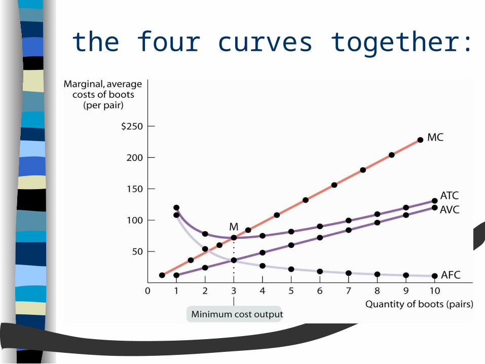
the four curves together:

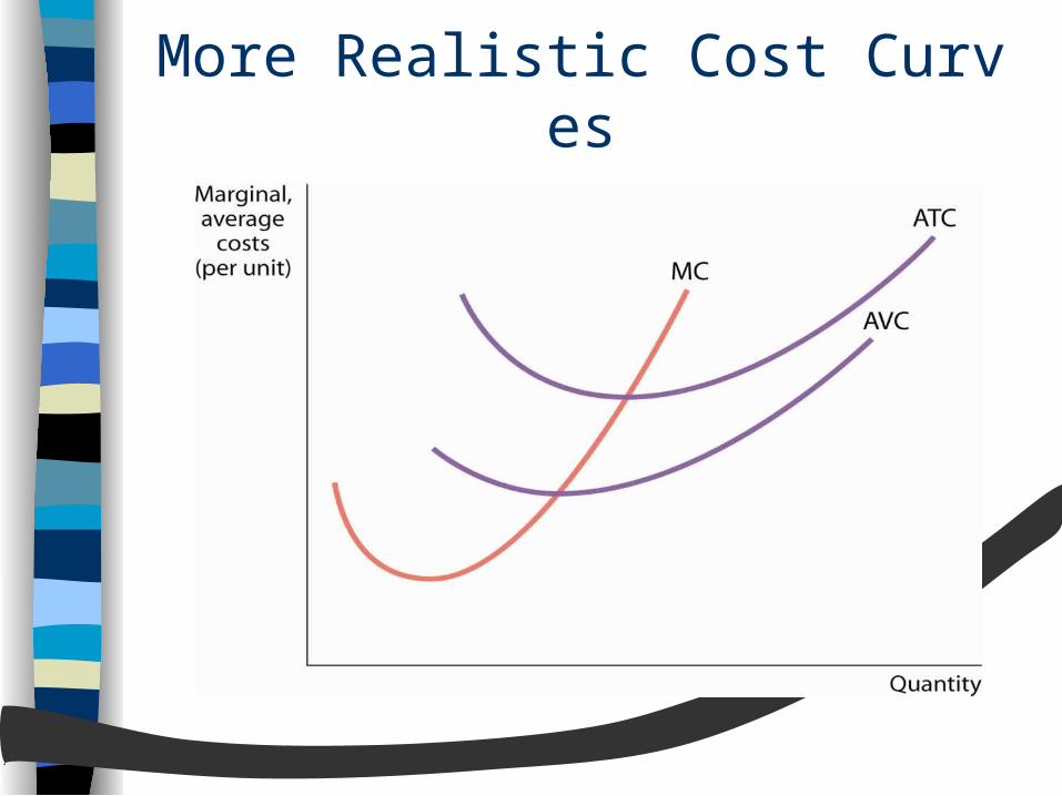
More Realistic Cost Curves

Total Revenue: TR

TR = PQ AR = PQ/Q = P MR = Δ(PQ)/ΔQ

= (ΔP*Q)/ΔQ + (P*ΔQ)/ΔQ= (ΔP /ΔQ ) Q + P(ΔQ/ΔQ )= (ΔP /ΔQ ) Q + PPerfect competition:MR = P = AR (ΔP =0)

Short-Run optimal output levelin a perfectly competitive market

Goal: maximize profit– Demand facing the industry: downward slo

ping– Demand facing the firm: horizontal at P

(all are price takers, and no one is large enough to affect market price)

Optimal output level determined by

D=P=MR=MC

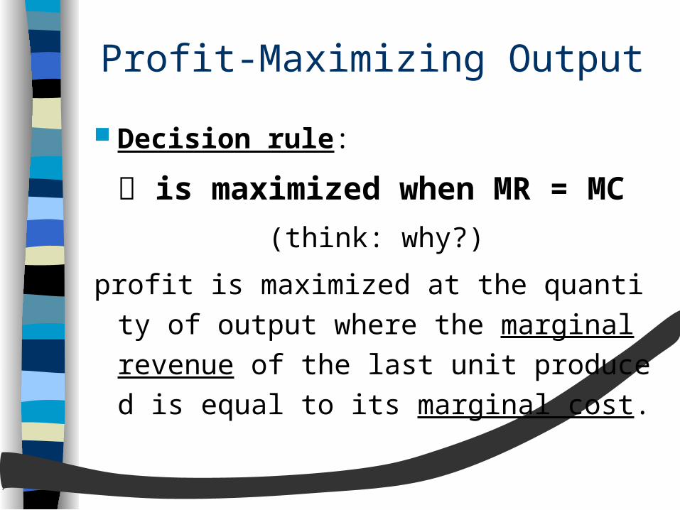
Profit-Maximizing Output

Decision rule:

is maximized when MR = MC

(think: why?)

profit is maximized at the quantity of outp

ut where the marginal revenue of the las

t unit produced is equal to its marginal c

ost.

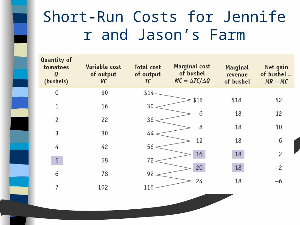
Short-Run Costs for Jennifer and Jason’s Farm

Questions to consider:

How much is fixed cost? Is marginal cost calculated based on tot

al cost or variable cost? Why is marginal revenue constant at $1

8? What is net gain? Is the goal to maximize net gain?

Again: under perfect competition

MR = Δ(PQ)/ΔQ

= (ΔP*Q)/ΔQ + (P*ΔQ)/ΔQ

= (ΔP /ΔQ ) Q + P(ΔQ/ΔQ )

When ΔP=0 (price taking)

MR =P

Decision rule:

is maximized when MR=P=MC

The Price-Taking Firm’s Profit-Maximizing Quantity of Output

The profit-maximizing point is where the marginal cost curve crosses the marginal revenue curve (which is a horizontal line at the market price).

Profitability and Market Price

Costs and Production in the Short-Run

Profitability and Market Price

The Short-Run Production Decision

A firm will cease production in the short-run if the market price falls below the shut-down price, which is equal to minimum average variable cost.

Short-Run optimal output level: various profit situations

Rule: produce at MR=P=MC.– Positive Economic Profit:

when D=MR=P>ATC at MR=P=MC– Operating at a loss:

when AVC<D=MR=P<ATC at MR=P=MC– Shut Down:

when D=MR=P<AVC at MR=P=MC

The break-even price:

the market price at which the firm earns zero profit (P=ATC).

P

Q

ATCMC

D=MR=P

AVCP1

P2

MR>MC, expand MR<MC, reduce MR=MC, optimal

Profit Maximization：MR=MC

Principles:

MC tells how much to produce (produce up to the amount where MR=P=MC)

ATC tells how much profit or loss is made if the firm decides to produce (profit = (P - ATC) * Q).

AVC tells whether to keep producing (keep producing only when P>AVC at P=MC)

Summary

Employeesper day

0 0 0 40

1 80 12 0.150 52 0.650

2 200 24 0.120 64 0.320

3 260 36 0.138 76 0.292

4 300 48 0.160 88 0.293

5 330 60 0.182 100 0.303

6 350 72 0.206 112 0.320

7 362 84 0.232 124 0.343

Bottlesper day

Variable cost

($/day)

Average variable cost

($/unit of output)

Total cost

($/day)

Average total cost($/unit of output)

0.15

0.10

0.20

0.30

0.40

0.60

1.00

Marginal cost

($/bottle)

Table 6.4, P.176Also example: AVC and ATC

The Marginal, Average Variable, and Average Total cost Curves for a Bottle Manufacturer

Price = Marginal Cost: The Perfectly Competitive Firm’s Profit-Maximizing Supply Rule

Measuring Profit GraphicallyFigure 6.7, P.178

A Negative ProfitFigure 6.8, P.179

The Short-Run Supply

A firm will cease production in the short-run if the market price falls below the shut-down price, which is equal to minimum average variable cost.

Short-Run Supply

for the firm: supply curve is upward sloping because of the law of increasing cost (S=MC).

for the industry: the supply curve is upward sloping, flatter than single firm supply curve, and steeper than the horizontal summation firm supplies.

The Short-Run Market Equilibrium

There is a short-run market equilibrium when the quantity supplied equals the quantity demanded, taking the number of producers as given.

The Effect of an Increase in Demand in the Short-Run and the Long-Run

D↑ P↑ non-zero profits entry S↑ P↓ back to zero profit

(on LRS curve)

Comparing the Short-Run and Long-Run Industry Supply Curves

The long-run industry supply curve is always flatter—more elastic—than the short-run industry supply curve. This is because of entry and exit:

Long-Run optimal output level:

All firms will be producing where P=LMC=LAC and economic profit will be zero because of free entry and exit.

Firms enjoy big economic rent if they own the resources that have higher productivity than similar resources owned by others.

LACLMC

AR=MRE

M

N

OQ

P

Long-Run Equilibrium

The Long-Run Market Equilibrium

A market is in long-run market equilibrium when the quantity supplied equals the quantity demanded, given that sufficient time has elapsed for entry into and exit from the industry to occur.

Conclusions:

In a perfectly competitive industry in equilibrium, the value of marginal cost is the same for all firms.

In a perfectly competitive industry with free entry and exit, each firm will have zero economic profits in long- run.

The long-run market equilibrium of a perfectly competitive industry is efficient: no mutually beneficial transactions go unexploited.

Long-Run Supply:

For the firm: produce where P=LMC=min LAC.

For a constant-cost industry: long-run supply is horizontal.

For an increasing-cost industry: long-run supply is upward sloping.