Production Economics of PrivateForestry: A Comparison ofIndustrial and Nonindustrial ForestOwnersDavid H. Newman and David N, Wear

This paper compares the producrion behavior of industrial and nonindustrial privateforestland owners in the southeastern U.S. using a restricted profit function. Profits aremodeled as a function of two outputs, sawtimber and pulpwood. one variable input,

regeneration effort. and two quasi-fixed inputs, land and growing stock. Although anidentical profit function is rejected, the results indicate behavior consistent with pmfit-

maximizing motives under both ownerships. The two ownerships have similar responsesto input and output price changes, both in the shon-run and in the long-run. However,nonindustrial owners appear to place a higher value on their standing timber and

forestland than do industrial owners. The difference in estimated shadow valuesindicates that significant nonmarket benefits are being captured by nonindustriai ownersand the benefits are reflected in their production behavior.

Key words: duality, forest production. restricted profit functions. timber supply and

demand elasticities.

A concern in the forestry literature is the per-ceived difference in production behavior be-tween industrially owned forest land and landmanaged by nonindustrial private forest (NIPJ?)owners (Clawson; Binkley; USDA Forest Ser-vice). For instance, in the southern United States,a large share of the region’s softwood timberproduction (35%) comes from the relatively smallshare of forested acreage (23%) owned by forestindustries. A much larger share of the region’sforest lands (67%) is held by NIPF owners, butthey produce a smaller share of the region’ssoftwood timber products (58%) from their lands(USDA Forest Service). Numerous public in-tervention attempts have been made to improveNIPF output (Boyd and Hyde).

The differences in relative output reflect dif-

she zwthon are associa te professor . Wamcll S c h o o l o f F o r e s t Rc-sources . The Un ivers i ty o f G e o r g i a . a n d economist. U S D A ForestService, Southeastern Fores t Erperimenf S t a t i o n . T h i s research wass u p p o r t e d by f u n d s pmvidcd by the U S D A F o r e s t S e r v i c e , South-castem Forest Enpcrimenr S t a t i o n . E c o n o m i c s o f Forest Pmrectiona n d Managcmcnt Research Unir. Research T r i a n g l e P a r k . N C . Theassismnce o f R a y S h e f f i e l d a n d D i a n n e RiSgsbee w i t h dara collcc-non i s acknowledged. H e l p f u l c o m m e n t s o n e a r l i e r d r a f t s w e r e re-wived from Joe Buongiomo. R’andy Rocker. Timothy Tzylor andt h i s Jownal’s reviewers.

R e v i e w coordinawd b y R i c h a r d Adans.

ferences in nianagement approach between the:two ownerships. Industrial forest lands, held by zfirms which also own wood processing facili- 3ties, are managed almost exclusively for timber 2production. On NIPF land, however, the pro- ,$duction of nontimber benefits may be of equal .gor greater importance than the production of ‘.:timber (Hartman; Binkley; Boyd).*In addition tothis choice of output mix, other ‘market fail-ure” reasons are attributed to NIPF landownersin order to reconcile their production decisions.These reasons include varying capital accessconstraints, technical ignorance, and even lackof profit motive (Kuuluvainen; Johansson andLofgren), which influence NIPF owne?’ re-sponse to market signals and therefore influenceregional timber production. Timber supply is-sues are increasingly important as timber inven-tories and production on large areas of pubIiclands in other regions are being reduced.

The purpose of the present study’ is-io test as-sertions concerning the production capabilitiesof NIPF and industriaf ownerships. Our hypoth-esis is that NIPF owners manage their land in amanner consistent with the profit motives main-tained by industrial owners. However, their pro-duction decisions involve additional consider-

Amrr. J. A.qr. Ewn. 75 (Augst 1993): 674-684Copyright 1993 American Agricultural Economics Asscxziation

l~e~mnn and Wear

ations beyond timber, such as nontimber goodsand services, and other factors which affect thelevel of timber outputs from their land. Thus,profit functions may differ between ownershipsas different management objectives are pursued.

We test this hypothesis using several proce-dures: (1) examine the first and second orderconditions for profit maximization using an es-timated restricted profit function for each own-ership; (2) statistically test for equivalent profitfunctions and, by duality, identical productiontechnologies between the two ownerships; (3)compare the implicit marginal valuation ofstanding timber and forest land under the twoownerships; and (4) compare restricted (short-run) and unrestricted (long-run) output supplyand input demand responses given shifts in rel-ative prices. Together, these tests provide in-sight into the modeling of timber markets andinto the appropriate design of policies aimed atincreasing timber production from privatesources.

Economics of PrivaJe FOXSJ~ 675

.,’ 5 Dual Model of Forestry Production

:i Following the approach used by Wear and New-j man to model the production behavior of in-- dustrial timber producers, we posit a multi-in-put, multi-output production (transformation)

: function for the forestry sector:

‘: ;I> TO’,, G,, R,, L,) = 0.i: : . .; Y is a vector of outputs, G is the level of timber. ,.; growing stocks, R‘is regeneration effort, L isforestland, and t indexes time. Growing stocksI ?ne viewed as an aggregate measure of accu-: mulated forestry capital adjusted through time1 by forest regeneration inputs, forest growth, andi; forest removals (outputs).:’ .i Long-run profit maximizing behavior by aI landowner can be modeled using the profit func-:,$on dual (n) to the transformation function:

.

ma byY - pRR - WGP~,-P~, PIY.GL.R

; GV, L, R, G-,); ..;t.5 ‘.’ : -P-tL;T(Y,G,L,R)=O]=O..: .‘: P+ -..;Profit maximization implies efficient intertem-;pOral allocation and (2) reduces the infinite se-krics of intertemporal decisions to a two-periodimodel similar to those presented by Max andikhan and Huhkrantz and Aronsson. The long-irun profit function is made up of three compo-CL..kg5 z;$A.It.‘.

nents: the first two terms define net pre-taxrevenues in the present period (product revenueminus regeneration cost); the third term definesthe expected value of timber growing stocks givencurrent output and variable input prices and dis:count rate (p); and the final term is the infinitestream of discounted land rents.

It may seem unusual to find no reference toharvest age in a model of forest production. Thisresult arises from the partial static equilibriumformulation and the underlying transformationfunction. Because we explicitly account forgrowing stock levels, the ratio of growing stocksto land exactly identifies the harvesting age ina partial equilibrium context. The aggregationof stand-level forest management problems to aforest firm with a fully regulated forest (uniformdistribution of age classes between zero and theharvest age) has been demonstrated by Comolli,based on insights deveIoped by Smith. Comol-li’s model allows the Faustmann rotation lengthproblem to be specified in terns of input andoutput quantities aione, facilitating standardcomparative statics analysis of timber supply.Furthermore, Comolli derives a firm-level profitfunction analogous to (2) from the stand-levelprobIem (pages 302-05, equation 11). For ourpurposes, partial equilibrium is a reasonable as-sumption for a region with a largely agriculturalforest sector (i.e. the U.S. South) but may be-come dubious when applied to an old-growthmining probiem (i.e. the Pacific Northwest).

The long-run forestry solution in the presenceof competitive markets for products and factorsalong with free entry defines a zero profit con-dition (Samuelson 1976; Comolli). However, thelong-run is best viewed as a target which wouldlikely never be attained (Kulatilaka). This is be-cause resource stocks, like most capital stocks.may not adjust instantaneously to short-run pricechanges. For example, adjustment in forest stocksis bounded from above by a biological growthprocess and, although land may be purchased orsold, the complement of growing stock on pdr-chased land cannot be perfectly controlled.

Given some exogenous price variability, thisslow adjustment process suggests that the con-ditions defined by (2) are only approached. Ac-cordingly, we define a restricted profit functionin which land and growing stocks are treated asquasi-fixed inputs to the forestry production .process and where outputs and regeneration in-

-put are treated as fully variable quantities.

(3) RI&p; G, L) = max [pry - pRR; GY.R

= G*, L = L*, T(Y. G, L. R) = O]

676 August 2993

where *‘s indicate existing leveis of the quasi-fixed factors.

The focus of the profit maximization formu-lation in (3) is the economics of timber produc-tion. However, forestland jointly produces othernontimber (and often nonmarket) forest goodsand services such as hunting, wind breaks, bird-watching, and other amenity values. It has been

from the analysis of the restricted profit function(3) to define long-run elasticities. This followsfrom the Le Chatelier principle that the long-runprofit function is an envelope of short-run profitfunctions. If L* and G* denote solutions to thelong-run problem and are elements of the vector2 of quasi-fixed inputs, then the followingequations will hold:

asserted-that the production of many important -nontimber outputs are proportional to the quan- (4.1) yJxP. P3

= V,,RL!(p; z) * [ -V=RII(p; z)j-’tity of existing growing stocks (Hartman) andthat NIPF owners are more concerned with theproduction and consumption of these nontimbergoods and services than are industrial owners.’Under these assertions, NIPF owners should dif-fer from industriai owners with respect to thenet annual price they expect from both their

(4.2) VPl,IT(p, pz) = - [V,RI’&p; dl-

(4.3)%JxP, P3 = V,,Rn(p; 2) f [V&Xp; 2)

- [-V,RiQ;z>I-‘I’- &&YP; 9

growing stocks [E(pc)] (equivalent to the timbervalue plus the nontimber goods and service value)and their bare land value (pd.

Because the profit function is restricted withrespect to growing stocks and land variables, wecan proceed without direct knowledge of theseamenity values or of the Iandowner’s personaldiscount rate. The marginal value (shadow price)of these inputs can be derived from the esti-mated restricted profit functions by taking thepartial derivative of the restricted profit functionwith respect to the leveis of quasi-fixed inputs.If land and growing stock quantities are at theiroptimal levels, then these shadow prices definerespective market rental prices (Samuelson 1953;Squires). Therefore, with quantities at the long-run solution defined in (2), the shadow price ofthe land input derived in (3) defines pL; theshadow price of G derived in (3) defines pG =E(P,; P, ~1.

The restricted profit function can also provideconsiderable information regarding the supplyof timber products and demand for forestry in-puts. The envelope condition allows the directderivation of short-run input demand and outputsupply responses for variable factors. In addi-tion, because restricted and unrestricted profitfunctions are dual to a common production tech-nology, an estimated restricted profit functioncan define long-run adjustments for both vari-able and quasi-fixed inputs (Lam Wear andNewman). Thus, given quantities at their opti-mal levels defined by (2), we can use the result<

.:’’ Industrial (as well as some NIPF) landowcts have begun to

market scmc of the non-timber values of their forest lands throughthe sale of hunting I-. However. industrial landowners primaryconsideration remains the ptoduction.of timber products and wea.ssutnc that these otha activities do noi impact their managunenrpl%l?..

where h’(p, pz) is the long-run profit functionand Vii is the gradient of this long run functionwith respect to input or output prices i and j.

These equations define long-run elasticities ofoutput supply and input demand for all quan-tities. While the length of time between the short-run and long-run is unspecified in a cross-sec-tional model (and could be as long as 20-30years for southern forestry), the long-run resultsprovide insight into the eventual price-respon-siveness of the two owuerships.

Data and Estimation Methods

The estimated model is a three-input, two-out-put restricted profit function for both industrialand NIPF ownerships in the Coastal Plain re-gion of the southeastern U.S. Data are cross-sectional, county level observations of industrialforest and NIPF acreage from five southeasternstates: Virginia, North Carolina, South Caro-lina, Georgia, and Florida. The data were com-piled primarily through surveys performed in eachstate by the U.S. Forest Service, SoutheasternForest Experiment Station, during the period from1984 to 1988. We limit the analysis to CoastalPlain southern pine production to address pro-duction units with similar production technolo-gies.

The variadie input, regeneration effort (R) isthe average annual acres planted to pine duri’ngthe survey’ period. We assume that capital andlabor are’ separable in fore& regeneration, allow-ing the use of an aggregate regeneration inputvariable. For each ownership in each county,acres of land in pine‘production (L) and volumeof pine growing stock (G) were also determinedand specified as quasi-fixed variables (all vol-

umes are in thousand cubic feet [mcf]). Aver-age annual outputs were separated into pinesawtimber, Ys (volume harvested from treesgreater than 9 inches in diameter), and pulp-wood, Y, (volume harvested from trees less than9 inches). Corresponding output prices (ps andpp) were taken from the quarterly Timber MartSouth stumpage price reports and averaged foreach state’s survey period (Norris). These pricesare reported by subregions in each state and wereassigned to counties within each subregion.

A unit cost index was constructed for regen-eration effort (pR) by taking the average priceof site preparation and planting for each county.Observations were costs reported by private landowners applying for federal cost share funds un-der the Forestry Investment Program (FIP) in1984. Some counties contained insufficient ob-servations to estimate a cost so that for thesecounties, costs were averaged with adjacentcounties. These costs are assumed to be similarfor both NIPF and industrial forest landownersbecause PIP required planting techniques simi-lar to those used on industrial lauds. However,NIPF owners receive federal subsidies for forestplanting which were estimated, on a per acrebasis, as the sum of all relevant federal subsi-dies for planting received by each state dividedby planted acres. The resulting average subsidyof $27 per acre was subtracted from the plantingcost for NIPF owners.’

In compiling these data, only counties in whichboth industrial and NIPF production occurredwere considered for inclusion in the analysis.Counties in which either zero acres were regen-erated or no sawtimber or pulpwood harvestsoccurred were excluded. The resulting datasetcontained observations for 132 counties.3 Tocorrect for heteroskedasticity between widelydiffering county sizes, each county’s quantityvariables were divided by the square root of thetotal southern pine acreage in that county. Wealso normalized the independent variables by theirsample means so that the point of expansion forOur second order approximation to the restricted

Economics of Privare Forestry 677

profit function is the unit vector. Summary sta-tistics for the data used in the analysis are pre-sented in table 1.

Restricted profit, defined as the net of productrevenue and total variable cost (regenerationcost), is estimated using a Generalized Leontieffunctional specification as a second-order approximation to the actual restricted profit func-tion. The specific function estimated is

* WC would have prefcmxl IO distinguish berwccn subsidized andttttsttbsidixd regcncration by NIPF owners but the requisite dataarC unavailable. About 30% of the total act-es planted by NlPF own-erS in the South in 1985 reccivcd federal subsidies (USDA Forcsr*ice. tables 2-12 and 2-14).

’ A total of 196 coastal pfain counties arc located in the 5 state%ion. Only 147 of dtcsc counties contain both industrial and NIPFf~stland. Fificcn counties were excluded due to an absence offOrestry activitics. The d&ted counties arc either urban or subur-% CprimariIy in Not-them Virginia and Florida). While these coun-ti may present intcrcsting economic questions. they were dropped(0 reduce cconomctric complexity.

( 5 ) Rfl(p;Z) = c 2 avpf”p;‘*i=S.P.R j=S.P.R

i is~G,~G p$ZiZj + c c Y,iPiq + ‘RI7. .=. i=S.P.R j=L.G

Following Hotelhng’s lemma, we obtain short-run output supply functions for sawtimber andpuipwood and a derived demand function for re-generation effort by taking the first derivative of(5) with respect to output prices and regenera-tion costs, respectiveiy. This gives the follow-ing equations:

(6.3)

-‘R = i-g., aRi@“2 + c YRjq + ER.j=L.G

Symmetry is imposed on the system by re-quiring the following: oii = cyji, pii = pi,, and rii= xi for all i and i. The ei in equations (5),(6.1), (6.2), and (6.3) represent the respectiveerror terms for each equation. The errors are as-sumed to occur contemporaneously as additive,joint normal disturbances with zero means. Suchcross-equation restrictions necessitate the si-multaneous estimation of this entire system of.equations. All right-hand-side variables are con-sidered exogenous. While prices would be en-dogenous at the sector level, -we did not con-sider this a problem given thatobservations arecross-sectional and that production units are smallrelative to the forest products sector as a whole.

Zellner’s seemingly unre la ted regress ion .method is used to estimate the eight equationsystem (the profit and derived equations for NIPFowners and the corresponding four equations forindustrial owners); the individual symmetry re-strictions are applied during the estimation pro-

6 7 8 August 1 9 9 3

I n d u s t r y

Mean

# Obs. 132R 2,052 1,896L 55 ,928 5 1,220G

58,12849,293 41,182 81,080

YS 2.408 1,904YP

3.6441,644 1,911 1.264

pR fbc. 116 4 4 8 9pr S/n-d 360 126 360

cess. While the derived supply and demand tions is 0.63 and the F value is 32.56. Theequations could have been estimated alone, the level critical value with 52 numerator andprofit function estimates were needed to evalu- denominator degrees of freedom is 1.52, indiate shadow prices and long-run elasticities. eating rejection of the zero-coefficient nul1 hy

We also tested the hypothesis of identical NIPF pothesis.and industrial profit functions and, implicitly, Profit maximization implies that the follow-identical production technologies. TO do this, ing properties are maintained by the estimatedwe compared models with and without cross- restricted profit function for each ownership type:ownership constraints on the system of equa- (1) it is nondecreasing in output prices and non-tions using an F-test. increasing in input prices; (2) it maintains sym-

metry of second-order price terms: (3) it pas;sesses a positive definite price Hessian matrix;

Estimation Resuits and (4) it maintains positive linear homogeneityin prices (Chambers, pp. 123-30 and 277-81).

Table 2 presents coefficients of the estimated re- We tested the first condition at sample meansstricted profit function for each ownership. These and rejected the null hypotheses of zero slopesresults are obtained using the combined data set. in favor of the alternative hypothesis of increas-Ten of the fifteen coefficients are significant at ing (decreasing) output (input) price gradientsthe 10% level or better for NIPF ownerships while for the restricted profit function for both own-tweIve are significant for the industrial equa- erships based on a one-tailed t-test at the 5%tions. To gau e overall model fit, we calculate

3leve1.4 We tested the second condition, sym-

the system R proposed by McElroy (as pre- metry. using a standard F test with 12 restric-sented by Judge et al., page 477) for systems of tions and 996 degrees of freedom.’ The calcu-equations: lated F value was 1.771 (with a critical F value’ .,

at the 1% level of 2.18) so that the imposition ‘-

where e are the GLS residuals, the numerator(2-l @ I) is the covariance matrix of the joint

, disturbance vector, and D, is a matrix for trans-forming y observations into deviations from their .respective means. The R2 value defines an F sta-tistic for the hypothesis of overall system sig- c a l c u l a t e d u s i n g the appropriate linear combination of the terms

nificance: from the vatiance-covariance matrix of the coefficients. The re-

R2 MT-Xi& 2.61 and 4.63: for pulpwood arc 2.04 and 1.81: and for rcgxe~

(8) F=-ation 2.28 and 2.46.

1 - R2 -ZiKi - M . ’ Th& degrees of freedom is equal to MT - K, when M equals -zthe number of equations (8). T equals the number of observations 2

The estimated R2 for the overall system of equa-per equation ( 1321. and K equals the number of explanatory vari- $ables (60). -?T

ifi

Newman and Wear Economics of Privare Foresrry 679

Table 2. Estimates of Coefficients for the Restricted Profit Function (equation 5) for bothIndustrial and NIPF Ownerships”

Ctws-Coefficient

price-s-priceassappai7a,am%.T

price-x-2YSGYSLYffiY?LYRGY.QL

z -x -z

Industry NIPF

Estimate S.E.b Estimate S.E.b

7 .12 1.43* 6.48 1.69*7.21 1.23* 4.24 1.08*1.35 1.00 5.34 1.08*

-3 .53 0.95’ -1 .26 0 .89-I .72 0.80* -1 .26 0.71-e- 0 . 3 9 0 .90 -3 .82 0.77*

1.69 0 . 9 1 ” 5.38. 1.18*1.83 0.92* 3.49 1.48*

-0 .61 0 .57 -0 .31 0 .573.44 0.58* 2.00 0.65*1.04 0.49* -0 .89 0.78

-4 .98 0.49* -4 .77 0.91*

1.99 0.76’ -1 .10 1.021.88 0.59’ -1 .24 1.23

-1 .48 0.68f 2.94 1.16’

’ Variables of the profit functionwe estimated simultaneously with the variable input demand and supply functions. Coefficients for theselatter f u n c t i o n s an: c o n t a i n e d i n t h e p r o f i t f u n c t i o n a n d arc t h u s n o t r e p e a t e d .’ S tar red var iab les ind icate significsnce level o f t h e e s t i m a t e d c o e f f i c i e n t .l i n d i c a t e s s i g n i f i c a n c e a t t h e 5 % l e v e l .

** ind ica tes s ign i f i cance a t the 10% l e v e l .

genvalues) held for all observations under bothownerships. The latter is not a statistical test ofthe second-order conditions. However, thesemathematical results, and the statistical resultsfor the first-order conditions of positive valuedoutput supplies and negative valued input de-mand, indicate that each ownership maintainsan estimated profit function consistent with aprofit maximization hypothesis. That is, profitsare positively related to output prices and neg-atively related to input prices.

The model (5) does not impose linear pricehomogeneity. Therefore, we tested for homo-geneity at sample means using model estimates.For homogeneity to hold,

RIl(Ap; Z) = ARIi’(p; 2).

In the present model,

RL’(hp; Z) = ARL’(p; Z)

+ ( 1 - A) c c &ZiZj.i=G.L j=C.L

S O

p;,z,z, = 0i=C.L j=G.L

is sufficient for linear homogeneity. We cannotreject price homogeneity using a two-tailed t-test at sample means at the 5% level under eitherownership (the t-values are 0.34 for industry and0.80 for NIPF).

We tested the hypothesis of identical profitfunctions between ownerships by comparing theconstrained and unconstrained equation sys-tems. The resulting F-statistic (constraints equal15 and the degrees of freedom equal 966) was4.03 (the critical value at the 1% level is 2.04),which indicates rejection of the null hypothesisof equivalent profit functions. Therefore, the es-timated equations are not consistent with anidentical profit function (or production technol-ogy) between industrial and NIPF ownerships.

Our working hypothesis suggested that dif-ferences in production behavior may be’ ex-plained by differences in the relative valuationof standing treesfor the production of nonmar-ket benefits or other constraints on production.We-examined this hypothesis by computing andcomparing the implicit valuation of growingstocks and land for each ownership. We com-puted these shadow values for the quasi-fixedfactors using average values for the exogenousvariables (normalized to unity) and the esti-

6S0 Augusr I993 Amer. 1. Agr.

mated ownership coefficients. We took the par-tial derivative of (6) with respect to the quasi-fixed factor and corrected this value for units bymultiplying by the ratio of the average heter-oskedasticity correction factor (fi = 326.12) tothe average value for the fixed input (see table1). For example, the growing stock shadow valueequation for producer k is, when evaluated atthe mean of the data

I -( 9 ) Pa =

1 i=G.L

4 2 YGjpJ (fil~~/looo)j=R.S.P I

= @(PC, + PGd + YSG + YPG

+ yR‘I(fi/c’t/ 1 oo”)

= [a'b](fJ/Gk/lOOO)

where a is a (5 X 1) vector of l’s and 2’s andb is a (5 X 1) vector of coefficients. The quasi-fixed factor is divided by 1000 because profit ismeasured in thousands of dollars. The resultingshadow values are therefore dollars per thou-sand cubic feet for growing stock and dollarsper acre for land. The estimated variance is cal-culated directly from the variance-covatiancematrix of the estimated coefficients (Q. Thus,for growing stock

(10) xpa* = (a'f2a)(lif/Gk/1000)'.

Because they are derived from the estimatedcoefficients of the restricted profit function, theshadow values should be interpreted as annualrental rates corresponding to E(pc) and pL in (2).For growing stock, NIPF owners maintain ashadow price of $31.97/mcf compared with avalue of $20.84/mcf for industrial owners. Forbare forest land, NIPF maintain a value of$23.17/ac compared to $6.38/ac for industry.It is difficult to validate these shadow priceswithout observations on the markets for clearedforest land and for forest stocks. Rough com-parison, however, suggests that these estimatesare reasonably ciose to available proxies. Usinga 5 percent interest rate, the capitalized growingstock values are $417 for industry and $639 forNIPF. These values fall between ‘the averagepulpwood and sawtimber prices as shown in ta-ble 1. Capitalized land prices are $127/ac forindustrial land and .$463/ac for NIPF. Wash-bum estimates values for cutover land in theGeorgia coastal plain range from %302/ac to

$497/ac between 1979 and 1988. Thesegia values would be relatively high cornthe region as a whole since the statestrongest forest sector.

We tested the hypothesis of identical shado&gprices for each of the fixed factors (2) betwe&?ownerships using a standard t-test: gjg

.:..-..J

(11)P2.N - P2.I

1= -:,:;g

.. :I

V*( pzvN)2 + s(p,*,)2 :-f$:c?. ..r

The t value for the difference between growing:stock values is 1.34; for land values it is 1.56. .;In both cases we can reject the hypothesis of .iidentical values at only the 20% level with a two iitailed test. .:

:The disparity between these values weakly ;

suggests there are differences between NIPF and 1industrial owners in perceived returns from their . _timber. An obvious candidate to explain thisdifference is that NIPF owners obtain substan-tial benefits from the timber remaining in place .and thus value their resources accordingly.: _’However, the differences shown in both thesevalues may also be related to the relative size ofthe forest tracts between these ownerships. Basedon limited transaction data of farm forestland,de Steiguer found the per acre sale value in-versely related to tract size. A smaller tract size ‘:could be expected to increase the rotation length ,.by raising harvesting costs and thus increase theopportunity cost on the standing timber (Com-olli). Since industrial owners favor much largertracts, the difference in the estimated shadowvalues may be related to this difference. Thesetypes of scale effects could not be effectivelymodeled with our data.

As a further comparison of ownership behav-ior, we used the estimated coefficients to com-pute the restricted (short-run) supply and de-mand elasticities at the mean values of thevariables (table 3). For instance, the formula forthe sawtimber elasticity for county k is

Variances were calculated using the method de-scribed in Dorfman,Kling, and Sexton. and Mil-ler, Capps, and Wells. The estimated own-priceelasticities, while significantly different from 0(except for industrial regeneration) are highlyinelastic for both ownerships. The respectiveelasticities are not significantly different be-tween the two ownerships. The ranking of out-

680 August 1993

mated ownership coefficients. We took the par-tial derivative of (6) with respect to the quasi-fixed factor and corrected this value for units bymultiplying by the ratio of the average heter-oskedasticity correction factor (fi = 326.12) tothe average value for the fixed input (see table1). For example, the growing stock shadow valueequation for producer k is, when evaluated atthe mean of the data

l-

( 9 ) PC.& =1 i=G.L

j==R.S.P

+ YRGIM/G/ 1 @W

= [a’b](I;i/G,/mo)

where a is a (5 X 1) vector of I’s and 2’s andb is a (5 X 1) vector of coefficients. The quasi-fixed factor is divided by 1000 because profir ismeasured in thousands of dollars. The resultingshadow values are therefore dollars per thou-sand cubic feet for growing stock and dollarsper acre for land. The estimated variance is cal-culated directly from the variance-covariancematrix of the estimated coefficients (0). Thus,for growing stock

(10) w&l2 = (a’lRa) (W/~JlOOO)2.

Because they are derived from the estimatedcoefficients of the restricted profit function, theshadow values should be interpreted as annualrental rates corresponding to E(pc) and pL in (2).For growing stock, NIPF owners maintain ashadow price of $31.97/mcf compared with avalue of $20.84/mcf for industrial owners. Forbare forest land, NIPF maintain a value of$23.17/ac compared to ,$6.38/ac for industry.It is difficult to validate these shadow priceswithout observations on the markets for clearedforest land and for forest stocks. Rough com-parison, however, suggests that these estimatesare reasonably close to available proxies. Usinga 5 percent interest rate, the capitalized growingstock values are $417 for industry and $639 forNIPF. These values fall between -the averagepulpwood and sawtimber prices as shown in ta-ble 1. Capitali&d..land prices are $127/ac forindustrial land and ‘$463/ac for NIPF. Wash-bum estimates values for cutover land in theGeorgia coastal plain range from %302/ac to

The disparity between these values weakly’suggests there are differences between NIPF andindustrial owners in perceived returns from theirtimber. An obvious candidate to explain thisdifference is that NIPF owners obtain substan-tial benefits from the timber remaining in placeand thus value their resources accordingly.:However, the differences shown in both thesevalues may also be related to the relative size ofthe forest tracts between these ownerships. Basedon limited transaction data of farm forestland,de Steiguer found the per acre sale value in-versely related to tract size. A smaller tract sizecould be expected to increase the rotation lengthby raising harvesting costs and thus increase theopportunity cost on the standing timber (Com-olli). Since industrial owners favor much largertracts, the difference in the estimated shadowvalues may be related to this difference. Thesetypes of scale effects could not be effectivelymodeled with our data.

As a further comparison of ownership behav-ior, we used the estimated coefficients. to com-pute the restricted (short-run) supply and de-mand elasticities at the mean values of thevariables (table 3). For instance, the formula forthe sawtimber elasticity for county k is

qS7s.k = -0.3 %P + aSR[ 1 A .Y5.k

Variances were calculated using the method de-scribed in Dorfman,Kling, and Sexton, and Mil-ler, Capps, and Wells. The estimated own-priceelasticities, while significantly different from 0(except for industrial regeneration) are highlyinelastic for both ownerships. The respectiveelasticities are not significantly different be-tween the two ownerships. The ranking of out-

$497/ac between 1979 and 1988. These Geosgia values would be relatively high Compared &the region as a whole since the state has -.fie?strongest forest sector. “?‘;T;

We tested the hypothesis of identical shado$?prices for each of the fixed factors (2) betwee&:ownerships using a standard t-test: 13

(11)P2.N - PZJ

t= ,Vs(p*A2 + S(P,J2

The t value for the difference between growing-stock values is 1.34; for land values it is 1.56.In both cases we can reject the hypothesis ofidentical values at only the 20% level with a twotailed test.

EJewnxan and Wear Economics of Private Forestry 681

Table 3. Restricted Output Supply and Variable Input Demand ‘Elasticities for Industrialand NIPF OwnershiDs’

With respect to clxingcs in p&e of

:. Eksticity o f Sawtimb;; Pu!pwood Rcgcneration.

Indosuy

! S a w t i m b c r:: P u l p w o o d

: Regeneration

-0.273' -.-0.246' -0.027(0.104) (0.080) (0.064)

-0.389* 0.579' -0.190**(0.141) (0.192) (0.111)0.034 0.150" -0.184

(0.081) (0.080) (0.130)

NIPF

: S a w t i m b c r.;‘.- Pulpwood‘.

> Regeneration

;

0.224*(O-of%

-0 .166(0.129)O-208*(0.053)

1:. ’ St23md variables indicate significance level of the cstimatcd elastic!I., l indicates significance af the 5% kvcI.:c ** indicates significance at the 10% Iced.3’x i. _i . .i_.t;;.7$ put elasticities appears correct because’ pulp-;. wood can be produced from growing stocks of-. nearly any age, while sawtimber is produced only1. from larger, older trees.

. The negative cross-price effects between out-:. puts indicate that, in the short-run, pulpwoodand sawtimber are gross substitutes. ‘These val-

:: ues are significantly different from 0 at the 5%T Ievel for industrial owners but not so for NIPF.Increasing stumpage prices increase regenera-- tion demands while increasing the cost of re-generation inputs decreases both sawtimber andpulpwood production.

1.. The unrestricted (long-run) supply and de-mand effects for the profit function for eachownership can be calculated using a two-stepprocess. First, market prices for both variableand quasi-fured quantities are used to derive theunrestricted, full equilibrium levels for each in-put. Then these derived levels are used as inputsin equations (4.1), (4.2). and (4.3) to computethe long-run price effects. We estimated the long-run supply and demand elasticities, by assumingthat the calculated shadow prices for%he quasi-fixed factors approximate the true equilibriumDues that these owners would face. This asisumption may be questionable given the widedispersion in these values between the two own-erships because these prices should approach eachOther in the long-run. Unfortunately, no market. .

-0.056 -0.169*(0.042) (0.043)0.332" -0.166

(0.179) (0.107)0.068 -0.277*

(0.043) (0.073)

iry: standard cmxs arc in parentheses.

values for the quasi-fixed factors were availablefor our use in this exercise.

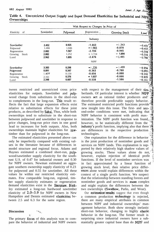
The estimated unrestricted elasticities areshown in table 4. Due to the numerical methodsusedtoe.stimatetheseelasticities,variances werenot calculated. Therefore, additional cautionshould be used in interpreting these values andthey are presented here to ailow for simple com-parisons between the short- and long-run. Allown-price elasticities display the anticipated signfor each ownership and NIPF owners show rel-atively less elastic own-price responses -for allinputs and outputs than do industrial owners. Inholding with le Chatelier, the absolute values oflong-run elasticities are substantially greater thantheir respective short-run values.

The magnitude of these long-run effects mayseem high when compared with the highly in-elastic short-run effects. What must be remem-bered is that the long-run in forestry is that pointin time when the quasi-fixed factors may becompleteIy adjusted in keeping with long-runprofit conditions (equation 2). Given the relativein@xibility. of the forest growth process, thiscan be many years. The recovery of the Southfrom a cutover and devastated timber region inthe 1930s to the leading forest products regionin the country by the 1970s supports the plau-sibility of these long-run values.

There are some interesting differences be-

6 8 2 Augusr 1 9 9 3

Elasticity of Sawrimber Regeneration

Indusrry

SawtimberPulpwoodRegenerationGrowing StockLand

2.4521.4662.0822.8822.962

0.9251.8461.5671.2521.895

- 1 . 6 6 3- I .985- 2 . 1 9 4- 1.724- 2 . 6 7 6

NIPF

- I .263- 0 . 8 7 0- 0 . 9 4 5- 1.894- .48.5I

Sawtimber 3.383 0.298 - I .326 - I .499PUlpWOOd 0.891 0.347 - 0 . 3 6 3 - 0 . 7 8 0Regeneration I .637 0.150 - 0 . 6 5 6 - 0 . 8 8 8Growing Stock 2.161 0.376 - 1.037 - 0 . 6 6 6Land 2.348 0.087 - 0 . 5 3 8 - 1 . 5 8 6

tween restricted and unrestricted cross priceelasticities for outputs. Sawtimber and puip-wood change from substitutes in the short-runto complements in the long-run. This result re-flects the fact that large expansion effects existrelative to substitution effects for these jointproducts, as described by Sakai. Thus, while bothownerships tend to substitute in the short-runbetween pulpwood and sawtimber in response toprice changes, long-run price rises in one goodlead to increases for both outputs. Also, bothownerships maintain higher elasticities for saw-timber than for pulpwood in the long-run.

The estimated elasticities presented above canonly be imperfectly compared with existing val-ues in the literature because of differences inmodel structure and regional focus. Adams andHaynes estimated a combined short-run, puip-wood/sawtimber supply elasticity for the south-east U.S. of 0.47 for industrial owners and 0.30for NIPF owners. Newman estimated an aggre-gate southern ownership supply elasticity of 0.23for pulpwood and 0.55 for sawtimber. All thesevalues lie within our restricted elasticity esti-mates. Few comparable long-run, regional, tim-ber supply elasticity estimates or regenerationdemand elasticities exist in the litenture. Bink-ley estimated a Iong-run hardwood sawtimberelasticity of 2.0-3.9 for NIPF owners in NewHampshire and Dennis estimated eIastic$ities be-tween 2.5 and 6.3 for the same region.

Discussion ‘- --.:: , _

The primary fzcus of this analysis was to com-pare the behavior of industrial and NIPF owners

with respect to the management of their tim-&;-:9

berlands. Of particular interest is whether NIPF iowners acf as rational timber producers and’ :therefore provide predictable suppiy behavior. ;‘-.

IThe estimated restricted profit functions provide””new insight into this issue. The first- and set- zT!lond-order conditions were met, indicating that 2NIPF behavior is consistent with profit max- yqimization. The NIPF profit function was found,..:3however, to be statistically different from the 9indusrry’s profit function, implying also that there i.2are differences in the respective production ..$technologies. . r.3

One expianation for the difference in behavior ,Jis the joint production of nontimber goods and :z$services on NIPF lands. This explanation is sup- .‘2ported by their relatively high shadow values of ..igrowing stocks. These values alone do not, -jhowever, explain rejection of identical profit $functions. If the level of nontimber services was jin fact approximated by a linear function of ;growing stock level, then relative price differ-ences alone would explain differences within the

:!

context of a single profit function. We suspectthat the relationship between standing forests andnontimber goods and services is more complexand might explain the differences between thetwo ownerships (SwalIow, Parks, and Wear).

Our estimatioti’results’ suggest that even thougha common production t&hnoiogy is rejected,there are many empirical attributes in commonbetween NIPF and industrial ownerships’ man-agement behavior. Both show strongly inelasticshort-run behavior, changing to highly elasticbehavior in the long-run. The former result issurprising since industrial owners have a sub-stantially greater capital base than do NlPF and

%' j-Je)+P~rl and WearB

_-

S should be able to respond more strongly to6 changing market conditions. Their relativelyg higher elasticities show that to some extent theyt do but they still appear constrained by other fac-F tot-s. These factors may be related to the factE;.s -that they also carry substantial investments ing downstream processing facilities /which needP continued, assured flows of raw material inputs.4.. In the long-run, both- industrial and NIPF$ owners will alter their mana%ement behavior tob take advantage of changed market conditions. Ag factor that is not addressed here is the length of

ftime between the short- and long-runs. If in-

F dust&l owners can adjust to the long-run morequickly, either because of larger capital re-sources or other factors, then their supply re-sponse to changing prices should be expected tobe higher and more rapid than for NIPF owners,as our results show.

The very inelastic, restricted price and cross-price elasticities of regeneration indicate thatforest owners are not greatly influenced in theirshort-run planting decisions by costs and prices.These results correspond to other studies show-ing minimal responsiveness (although some-what larger than the values shown here) in re-generation practices from prices for NIPF owners(Boyd; Royer). However, the long-run results,which have not been previously estimated, showthat regeneration demand will respond quitestrongly to permanent price changes.

Such changes from the short-run to the long-run present a conundrum for analysts assessingthe impact of measures designed to increasetimber production by lowering management costs(or perhaps to meet other social objectives byadding environmental or regulatory constraints,thus raising costs). A short-run analysis is un-likely to show substantial diit effects from theseefforts as management plans are already in place.The long-term impacts, however, may in fact bequite large. Our results do not comment on ef-ficiency aspects of forestry incentive programsor environmental regulations but they do indi-cate that these pro,ms can have large long-runimpacts.

We reject the hypothesis that NIPF landown-ers do not respond to price signals. The econo-metric tests for profit maximizing behavior are

Economics of Private Forestry 683

either receive substantial nonmarket (or non-measured) benefits from liolding timber in place,have differing expectations regarding futureprices, or hold a different opportunity cost ofcapital-

The suggestion that NIPF owners are satisfi-cers who eschew standard profit maximizing be-havior for greater overall satisfaction may wellmiss the p6int. Ouf’analysis, as have others be-fore, suggests that NIPF owners react to chang-ing market conditions in a manner consistent witha firm with an expanded (i.e. beyond just timberoutputs) transformation function. While they mayincorporate nonmarket values and other con-straints into their decision set they see clearlythe trade-offs in their timber land managementdecisions and act accordingly. Future researchmust include such external benefits and con-straints into market-based supply functions.

[Received January 1991; jimI revkionreceived October 1992 .]

References

Adams. D. M., and R. W. Haynes. -The 1980 SoftwoodTimber Assessment Market Model: Structure, Projectsand Policy Simulations.” Foresr Sci. Monograph 22.1980.

Baxter. N. D., and J. L. Cragg: ‘Corporate Choice AmongLong-Term Financing Instrumems.” Rev. Econ. and.%a&. 52(August 1970)~225-35.

Binkley. C. S. Timber Supply from Private Nonindustrial

Forests: A Microeconomic Analysis of Landowner Be-havior. New Haven: Yale Univ. School of Forest. andEnvir. Stud. Bull. No. 92. 1981.

Boyd. R. ‘Government Support of Nonindustrial Produc-tion: The Case of Private Forests.* South. &con. 1.Sl(July 1984):89-107.

Boyd. R.. and W. F. Hyde. Forestry Sector Intervention.

Ames, IA: Iowa State Univ. Press, 1989.Clawson, M. The Economics of U.S. Nonindustrial Private

Forests. Washington; DC: Resources for the Future.Research Paper R-14.

Comolli. P. M. ‘Principles and Policy in Forestry Eco-nomics.” Bell J. &on. lZ(Junc 198 1):300-09.

Dermis, D. F. ‘An Economic Analysis of Harvest Behav-ior: Integrating Forest and Ownership Characteristics.”Forest Sci. 35(Dwcmber 1989):1088-l 104.

Dorfman. J. H.. C. L. Kling. and R. J. Sexton. ‘Confi-all significant and their supply and demand re- I.?sponses are consistent with industrial owners. dence Intervals~for Elasticities and Flexibilities: Reev-

Our results do suggest that NIPF owners value aluating the Ratios of Normals Case.” Amer. /. Agr.

their timber resource in a different manner than.&on. 72(Novcmber 1990):1006-17.

industrial owners. The shadow values that NIPFFaustmann, M. 1849. Calculation of the Value Which Forest

Land and Immature Stands Possess for Forestry,’ inowners place on their timber and forestland assets M. Gane. ‘Martin Faustmann and the Evolution ofare substantially higher than the corresponding Discounted Cash Flow.” pp. 27-55. Oxford: Com-values on industrial lands. This suggests that they monwealth Forestry Institute Paper No. 42, 1968.

684 August 1993

Haz~~~an, R. ‘The Harvesting Decision Wben a StandingFonst has V&e.” Econ. fnquiry I4(Mar& 1976):52-58.

Hultkmna. L., and T. Arousson. ‘Factors Affecting theSupply and Demand of Timber from Rivare Nonin-dustrial Lands in Sweden: An Econometric Study.’Foresr Sci. 35(Decemher 1989):946-61.

Johansson. P. 0.. and K. G. Lofgren. The Economics ofForestry and Natural Resources. New York: BasilBlackwell, 1985.

Judge. G. G., W. E. Griffnhs, R. C. Hill. W. E. Lutkepoi.and T. C. Lx. The Theory and Practice of Econo-metrics. 2nd Ed. New York Wiley, 1985.

Kulatilaka. N. *The Specification of Partial Static Equilib-r i u m M o d e l s . ” R e v . Econ. and .Sfu~isr. 69(May1987):327-35.

Kuuluvainen. J. “Virtual Price Approach to Short-TermTimber Supply under Credit Rationing.” /. Environ.Econ. and Manag. 19(September 1990):109-26.

Lau, L. J. “A Characterization of the Normalized Re-stricted Profit Function.” J. Econ. Theory 12(February1976):131-63.

Max, W., and D. E. Lehman. *A Behavioral Model ofTimber Supply .” 3. Envi ron . Econ. and Manng.15(March 1988):71-86.

Miller. S. E.. 0. Capps, and G. Wells. ‘Confidence In-tervals for Elasticities and Rexibilities from LinearEquations.‘ Amer. 1. Agr. Econ. 66(August 1984):392-96.

Newman, D. H. ‘An Econometric Analysis of the SouthernSoftwood Stumpage Marker 1950- 1980. ” Foresr Sci.33(December 1987):932-45.

3

Norris, Frank W. Timber Mart South. (variOU.5 years) .gRoyer, J. P. -Determination of Reforestation Beha,+&?

Among Southcm Landowners.’ Foresr s .-%CL-733(Scptember 1987):654-67. ,>,+

Saksi, Y. ‘Subsritution and Expansion Effects in Produi?tion Theory: The Case of Joint Production.” J. Eco,$~Theory 9(July 1974):255-74.

.-. .9i, 5:<...,iSamuelson, P. A. ‘Prices of Factors and Goods in General“.:

Equilibrium.* Rev. Econ. Sfud. 21(January 1953):1,‘420. i ;.‘: 2

Amer. J. Agr.

-_ “Economics of Forestry in an Evolving Swiety.*:jEcon. Inquiry 14(December 1976):466-92. ! C-f

Smith, V. L. lnvesrmenf and Producrion: A Study in &‘aTheory of Capiral-Using Enterprise. Cambridge, ~ :.Harvard University Press, 1961. : 3

Squires. D. “Long-Run Profit Functions for Multiproduct !iFiis.* Amer. 1. Agr. Econ. 69(August 1987):558- ‘169. :S

.?de Stciguer. J. E. ‘Forestland Market Values.” J. Forestry ‘tg

8OfAprii 1982):214-16.‘C

ccSwallow, S. K.. P. I. Parks, and D. N. Wear. ‘Policy- 2

Relevant Nonconvexitia in the Production of Multiple fForest Benefits .” J . Env i ron . Econ. and Manag. I19(November 1990):264-80. :;

Washburn. C. L. The Dererminanrs of Forest Value in the’ iU.S. Sourh. Ph.D. Thesis. Yale University, 1990. <

Wear, D. N.. and D. H. Newman. *A Profit Function Ap-preach to Measuring the Production Structure of For- “’esuy.” Foresr .Sci. 37(June 1991):54@-5 1.

. _. .USDA Forest Service. The Sourh’s Fourth Fores?: Alter- :

norives for rhe Future. Washington DC: USGF’O. For- ‘:es Resource Report No. 24. 1988. ;’