production new
TRANSCRIPT
8/3/2019 Production New
http://slidepdf.com/reader/full/production-new 1/26
Production theory
Provides framework foreconomics of production of
firm

8/3/2019 Production New
http://slidepdf.com/reader/full/production-new 2/26
What is production
Production refers to transformation of inputs or resources into outputs of goodsand services
Inputs = resources used in production of goods (fixed and variable)
Output = end result
8/3/2019 Production New
http://slidepdf.com/reader/full/production-new 3/26
Basic production decision
1.How much of commodity to produce
2.How much inputs should be used
To answer these questions, the firm
a. Requires engineering data on productionpossibilities
b. Economic data on input and output prices
8/3/2019 Production New
http://slidepdf.com/reader/full/production-new 4/26
Production function
Production is a function that transformsinputs into output
Q = f (L, N, K……T)
Factors affecting production are
1.Technology
2.Inputs (land, labour etc)3.Time period (short run vz long run)

8/3/2019 Production New
http://slidepdf.com/reader/full/production-new 5/26
1) Total Product:
3) Marginal Product:
2) Average Product:
TP = Q = f(L)
MPL =
TP
L
APL =TPL
Production function with one variable
input

8/3/2019 Production New
http://slidepdf.com/reader/full/production-new 6/26
Concepts of production
Total Product :This is amount of totaloutput produced by a given amount of factor, other factors held constant.
Average Product: This is total outputproduced per unit of factor employed
AP =TP/no. of units of factor employed
Marginal Product: This is addition to totalproduction by employment of extra unit of factor
8/3/2019 Production New
http://slidepdf.com/reader/full/production-new 7/26
Law of variable proportions or law of
diminishing returns
As more and more of one factor input isemployed, all other input quantities heldconstant, a point will be reached whereadditional quantities of varying input willyield diminishing marginal contribution tototal product
Short run law
Some factors fixed, other factors variable State of technology fixed and unchanged
Possibility of varying proportion of factors
8/3/2019 Production New
http://slidepdf.com/reader/full/production-new 8/26
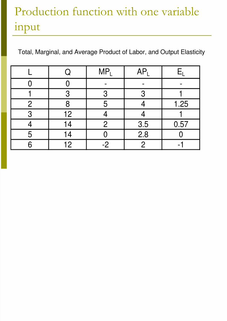
L Q MPL APL EL
0 0 - - -
1 3 3 3 1
2 8 5 4 1.25
3 12 4 4 1
4 14 2 3.5 0.57
5 14 0 2.8 0
6 12 -2 2 -1
Total, Marginal, and Average Product of Labor, and Output Elasticity
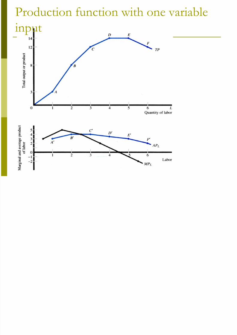
Production function with one variable
input
8/3/2019 Production New
http://slidepdf.com/reader/full/production-new 9/26
Production function with one variable
input
8/3/2019 Production New
http://slidepdf.com/reader/full/production-new 10/26

8/3/2019 Production New
http://slidepdf.com/reader/full/production-new 11/26
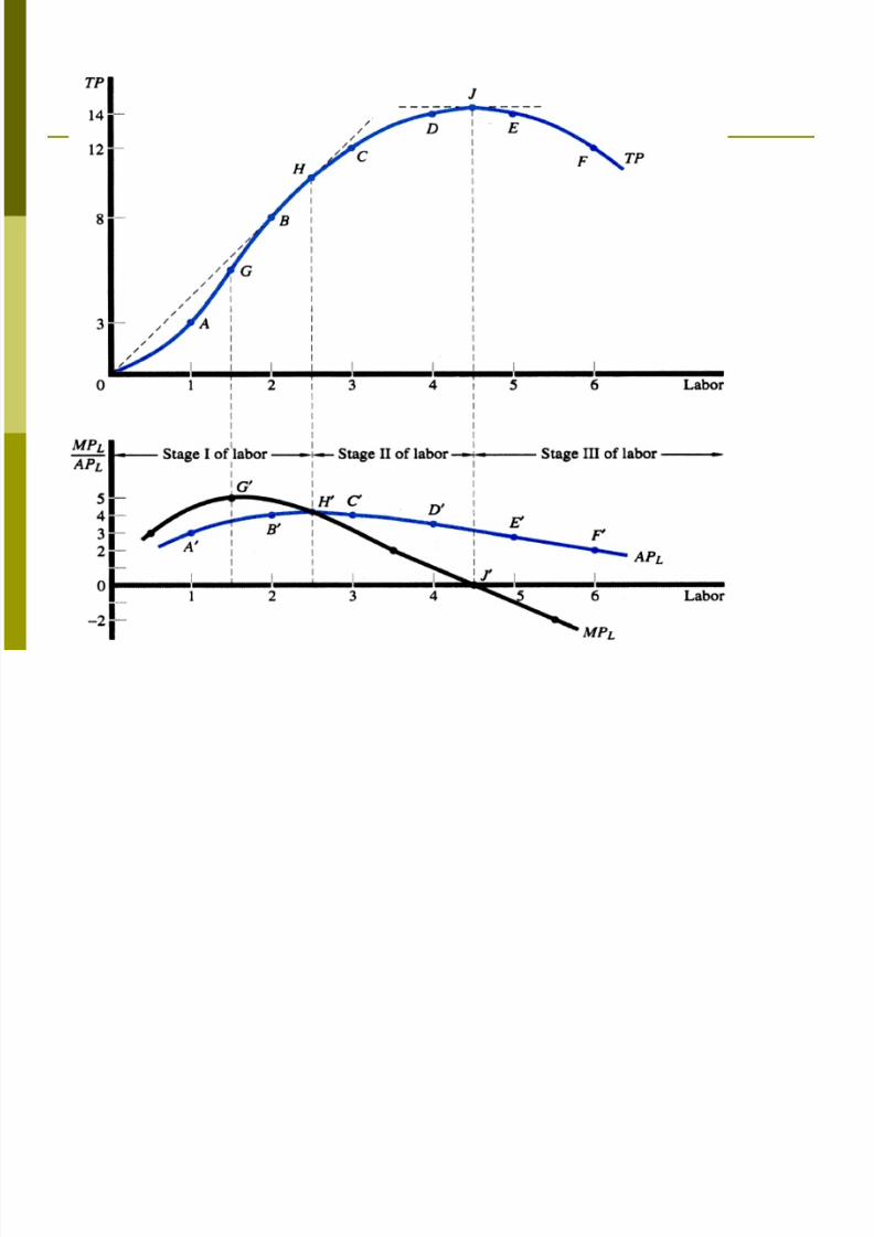
Stages of return
Stage 1:Increasing returns. MP increasing,AP increasing, TP increases till G atincreasing rate, after that at decreasing
rate. G= point of inflexionStage 2:Diminishing returns. MP decreasing
and falls till zero, AP decreasing, TPincreases at a decreasing rate
Stage 3:Negative returns. MP negative, APdecreasing, TP is also falling
8/3/2019 Production New
http://slidepdf.com/reader/full/production-new 12/26
Contd..
Stage of operations –stage2
Stage 1 – fixed factor too much forvariable factor. Fixed factor is more
intensively utilised Stage 3- variable factor too much in
relation to fixed factor
Applications – agriculture, studying
8/3/2019 Production New
http://slidepdf.com/reader/full/production-new 13/26
Isoquants show combinations of two inputsthat can produce the same level of output.
Firms will only use combinations of twoinputs that are in the economic region ofproduction, which is defined by the portionof each isoquant that is negatively sloped.
Production with two variable inputs

8/3/2019 Production New
http://slidepdf.com/reader/full/production-new 14/26
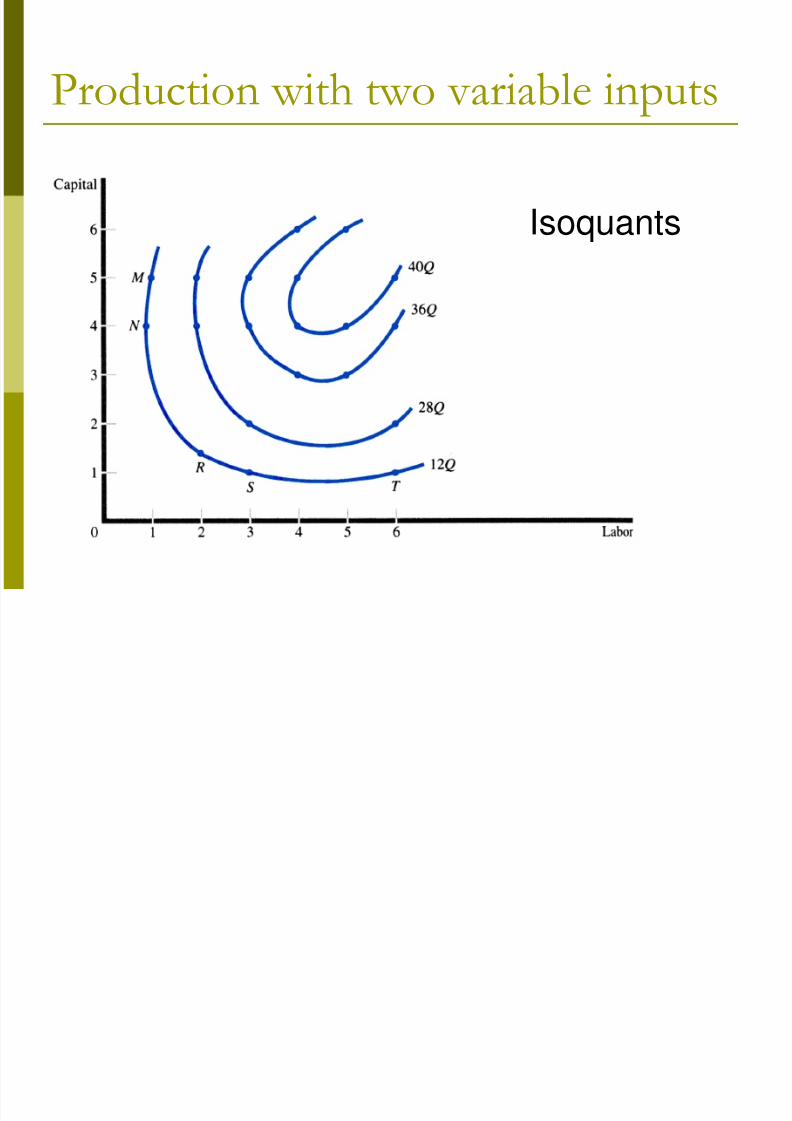
Isoquant
An isoquant is a curve representingvarious combinations of 2 inputs thatproduce the same level of output
ISO+QUANT= same + quantity
8/3/2019 Production New
http://slidepdf.com/reader/full/production-new 15/26
Isoquants
Production with two variable inputs
8/3/2019 Production New
http://slidepdf.com/reader/full/production-new 16/26
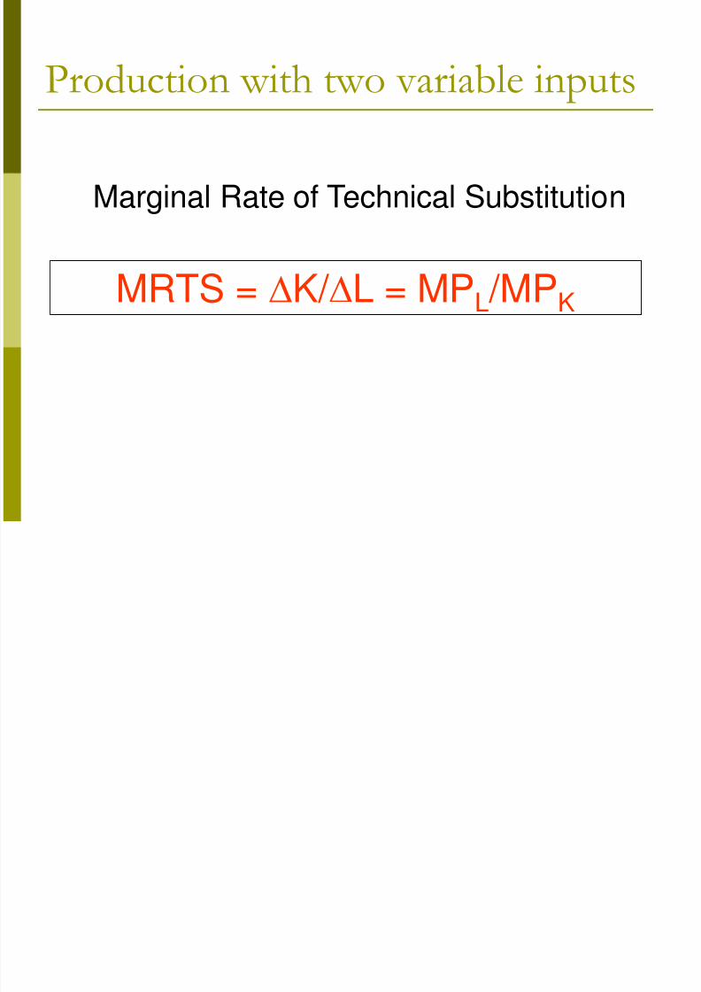
Marginal Rate of Technical Substitution
MRTS = K/ L = MPL /MPK
Production with two variable inputs
8/3/2019 Production New
http://slidepdf.com/reader/full/production-new 17/26
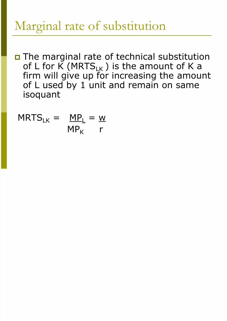
Marginal rate of substitution
The marginal rate of technical substitutionof L for K (MRTSLK ) is the amount of K a
firm will give up for increasing the amountof L used by 1 unit and remain on sameisoquant
MRTSLK = MPL = wMPK r

8/3/2019 Production New
http://slidepdf.com/reader/full/production-new 18/26
Production With Two
Variable InputsMRTS = (-2.5/1) = 2.5
8/3/2019 Production New
http://slidepdf.com/reader/full/production-new 19/26
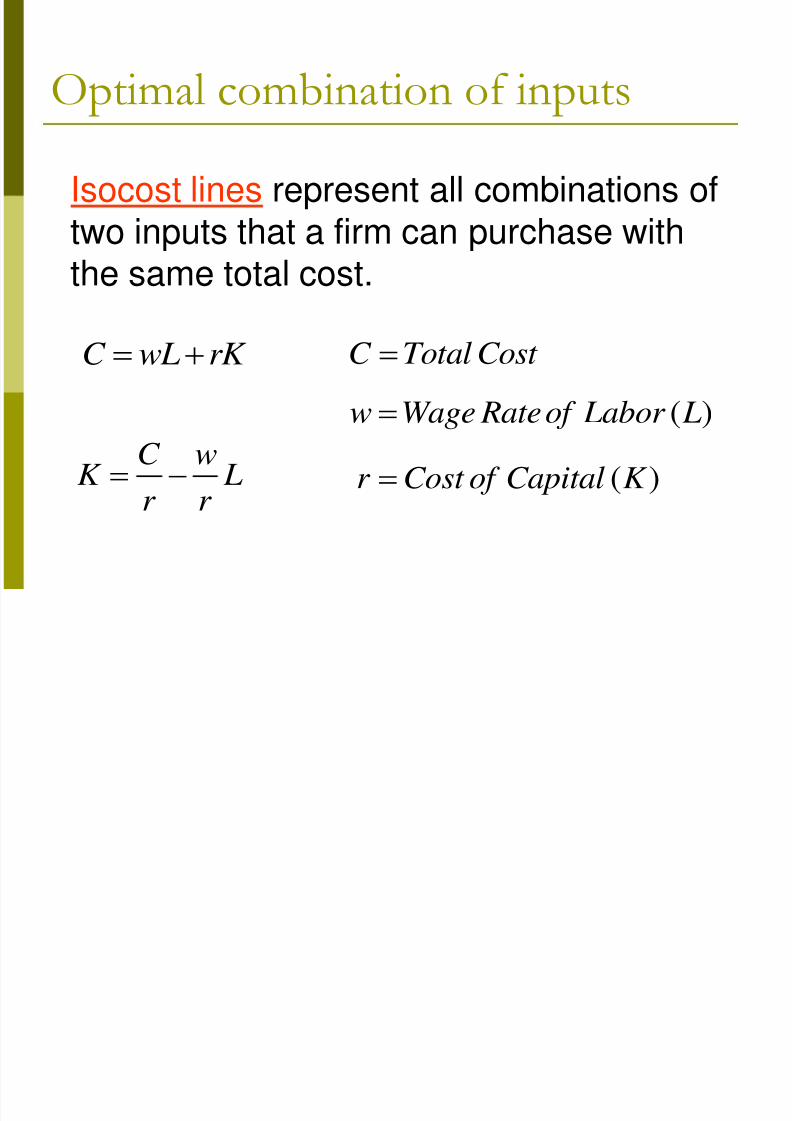
Isocost lines represent all combinations oftwo inputs that a firm can purchase with
the same total cost.
C wL rK
C wK L
r r
C Total Cost
( )w Wage Rate of Labor L
( )r Cost of Capital K
Optimal combination of inputs
8/3/2019 Production New
http://slidepdf.com/reader/full/production-new 20/26
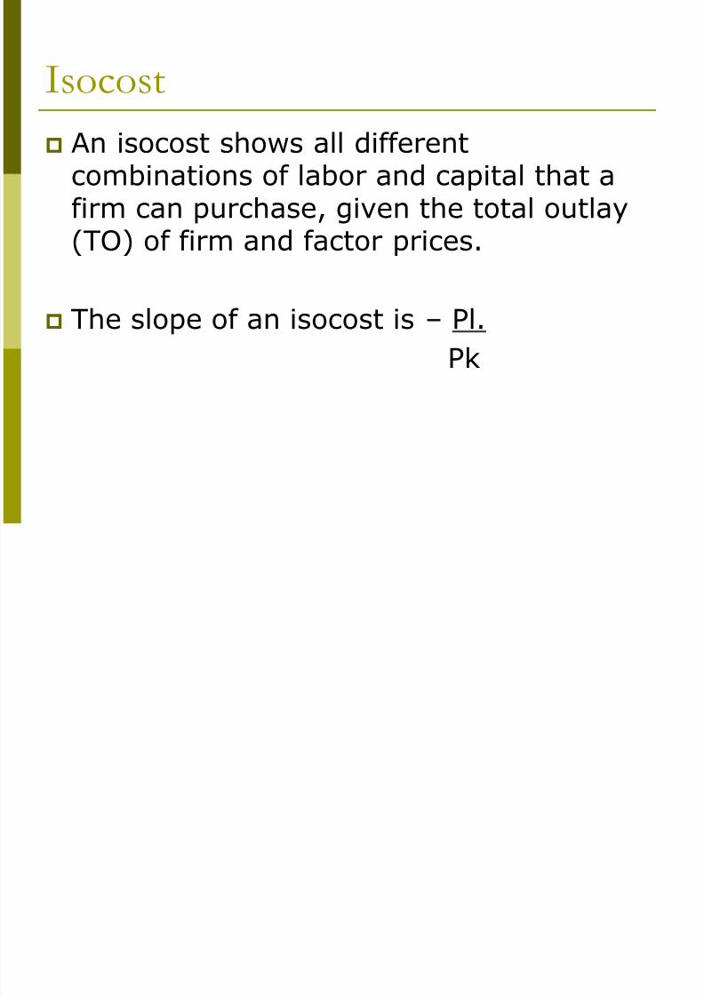
Isocost
An isocost shows all differentcombinations of labor and capital that afirm can purchase, given the total outlay
(TO) of firm and factor prices.
The slope of an isocost is – Pl.
Pk
8/3/2019 Production New
http://slidepdf.com/reader/full/production-new 21/26
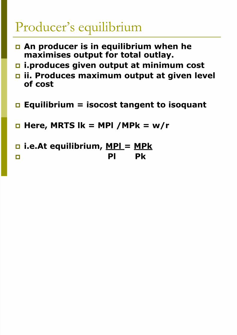
Producer’s equilibrium
An producer is in equilibrium when hemaximises output for total outlay.
i.produces given output at minimum cost
ii. Produces maximum output at given level
of cost
Equilibrium = isocost tangent to isoquant
Here, MRTS lk = MPl /MPk = w/r
i.e.At equilibrium, MPl = MPk
Pl Pk
8/3/2019 Production New
http://slidepdf.com/reader/full/production-new 22/26
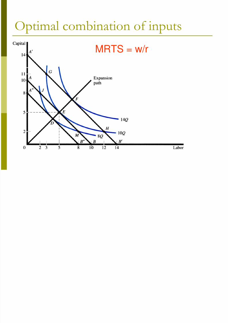
MRTS = w/r
Optimal combination of inputs

8/3/2019 Production New
http://slidepdf.com/reader/full/production-new 23/26
Production Function Q = f(L, K)
Q = f(hL, hK)
If = h, then f has constant returns to scale.
If > h, then f has increasing returns to scale.
If < h, the f has decreasing returns to scale.
Returns to Scale- Change in all inputs
8/3/2019 Production New
http://slidepdf.com/reader/full/production-new 24/26
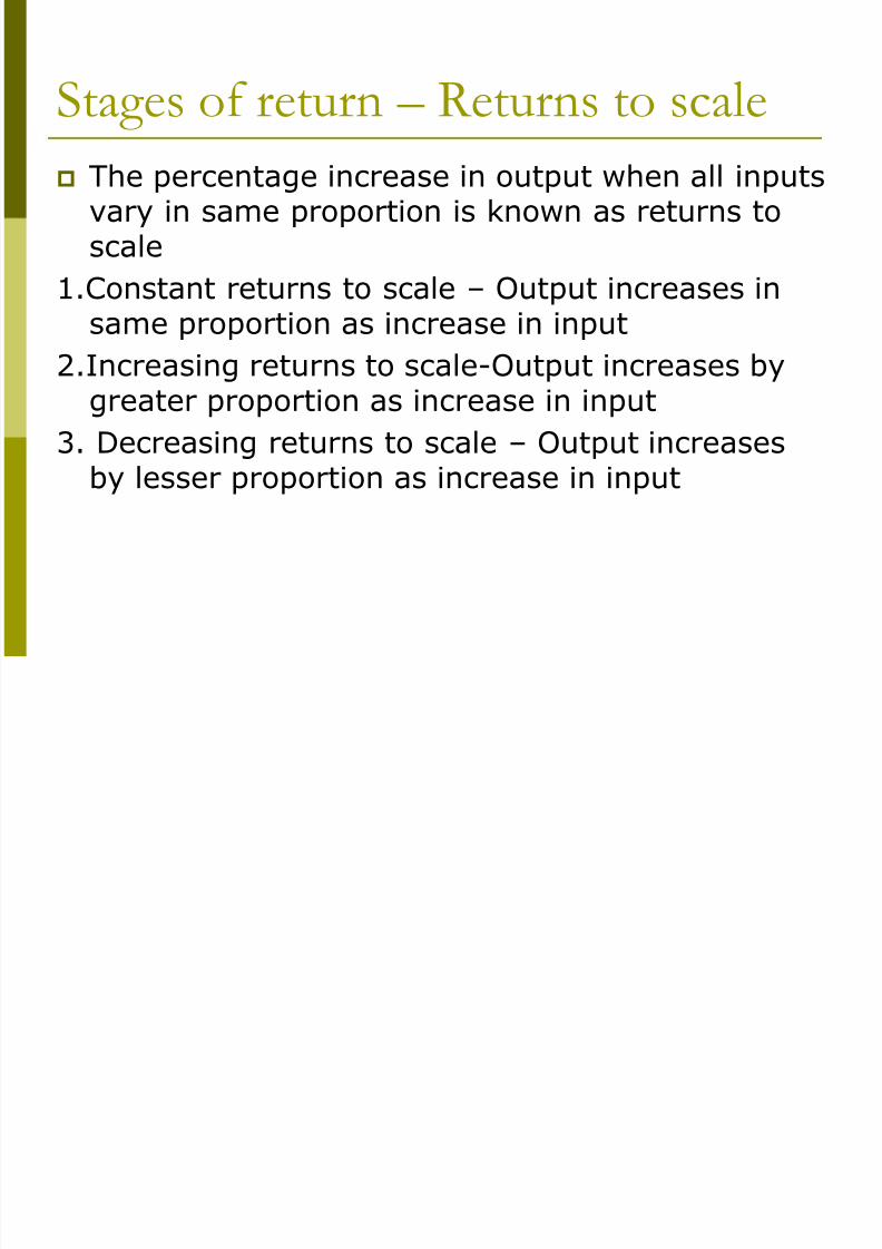
Stages of return – Returns to scale
The percentage increase in output when all inputsvary in same proportion is known as returns toscale
1.Constant returns to scale – Output increases insame proportion as increase in input
2.Increasing returns to scale-Output increases bygreater proportion as increase in input
3. Decreasing returns to scale – Output increasesby lesser proportion as increase in input
8/3/2019 Production New
http://slidepdf.com/reader/full/production-new 25/26
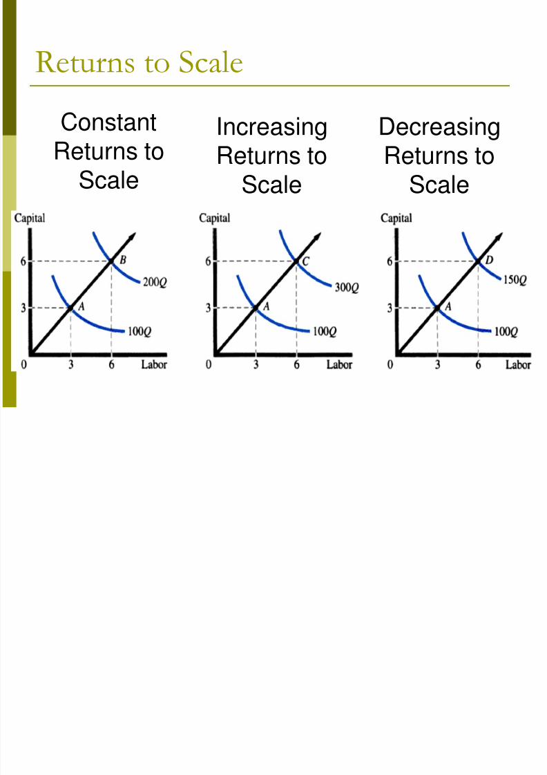
ConstantReturns to
Scale
IncreasingReturns to
Scale
DecreasingReturns to
Scale
Returns to Scale
8/3/2019 Production New
http://slidepdf.com/reader/full/production-new 26/26
Reasons
Causes of increasing returns
Specialisation in large scale production. Insome industries, small scale production is
not possible
Causes of decreasing returns
Coordination and control maybe difficult.Information maybe lost or distorted whentransmitted