production operations management portfolio (p om) … · production operations management portfolio...

Production Operations Management Portfolio (POM)

Curtis Hubbard Jr.

MGNT 3185, M-F 12:00p.m.-01:50p.m.

Table of Contents

I. Computer Lab Assignment #1

a. Cover Page

b. Explanatory Paragraph

c. Appendix A

II. Computer Lab Assignment #2

a. Cover Page


c. Appendix A

III. Computer Lab Assignment #3

a. Cover Page


c. Appendix A

IV. Computer Lab Assignment #4

a. Cover Page


c. Appendix A

V. Computer Lab Assignment #5

a. Cover Page


c. Appendix A

VI. Computer Lab Assignment #6

a. Cover Page


c. Appendix A

VII. Computer Lab Assignment #7

a. Cover Page


c. Appendix A

VIII. Computer Lab Assignment #8

a. Cover Page


c. Appendix A

Computer Lab Assignment #1

Curtis Hubbard Jr.

MGNT 3185, MW 06:00-07:15p.m.

Explanatory Paragraph for Computer Lab Assignment #1

Using the Management Scientists software a 3-month Simple Moving Average (SMA)

forecast and an Exponential Smoothing (ES) forecast were conducted. The Mean Squared Error

(MSE) for ES was 329.81 while the MSE for SMA was 296.11. The SMA is the superior

forecasting technique, because it has a lower MSE. The forecast for period 9 using the SMA

forecasting technique was 758.67.

FORECASTING WITH MOVING AVERAGES********************************

THE MOVING AVERAGE USES 2 TIME PERIODS

TIME PERIOD TIME SERIES VALUE FORECAST FORECAST ERROR=========== ================= ======== ==============

1 7702 7973 790 783.50 6.504 782 793.50 -11.505 765 786.00 -21.006 702 773.50 -71.507 700 733.50 -33.508 759 701.00 58.00

THE MEAN SQUARE ERROR 1,702.33

THE FORECAST FOR PERIOD 9 729.50


Curtis Hubbard Jr.

MGNT 3185, MW 06:00-07:15p.m.


Ft= 143.8 + 1.945t

Using the Management Scientist software a linear trend equation was developed. If no

units were sold then big T would equal 143.8 units sold. If little t were equal to 18, then big T

would equal 178.81 units sold (143.8 + 1.945(18) = 178.81 units sold). The forecast for period

20 is 182.70 units sold.

FORECASTING WITH LINEAR TREND*****************************

THE LINEAR TREND EQUATION:

T = 150.067 + 0.697 t

where T = trend value of the time series in period t

TIME PERIOD TIME SERIES VALUE FORECAST FORECAST ERROR=========== ================= ======== ==============

1 166 150.76 15.242 148 151.46 -3.463 150 152.16 -2.164 147 152.86 -5.865 155 153.55 1.456 144 154.25 -10.257 155 154.95 0.058 146 155.64 -9.649 150 156.34 -6.3410 178 157.04 20.96

THE MEAN SQUARE ERROR 96.28THE FORECAST FOR PERIOD 11 157.73THE FORECAST FOR PERIOD 12 158.43THE FORECAST FOR PERIOD 13 159.13THE FORECAST FOR PERIOD 14 159.83THE FORECAST FOR PERIOD 15 160.52THE FORECAST FOR PERIOD 16 161.22THE FORECAST FOR PERIOD 17 161.92THE FORECAST FOR PERIOD 18 162.61THE FORECAST FOR PERIOD 19 163.31THE FORECAST FOR PERIOD 20 164.01


Curtis Hubbard Jr.

MGNT 3185, MW 06:00-07:15p.m.


Y= 4.517+ 1.627X

A regression analysis was conducted to determine if the bus and trolley ridership demand

has any relationship to the number of tourists visiting TyTy, Georgia on an annual basis. The

significant predictor of the omnibus F-test is .001. The coefficient of determinants (r2) is .821.

This confirms that approximately 82% of the variability in the dependent values can be

determined by the independent variable. The coefficients of correlation is .906, indicating that

there will be a strong positive relationship between the two variables. If there are no tourists the

predicted ridership will be 4.517. If 11 million people visit the city the predicted ridership will be

approximately 17,897,005.

DECISION ANALYSIS*****************

YOU HAVE INPUT THE FOLLOWING PAYOFF TABLE:******************************************

STATES OF NATUREDECISION 1 2******** ****** ******

1 220000 -18000

2 116000 -21500

3 0 0

PROBABILITIESOF STATES 0.300 0.700

DECISION RECOMMENDATION***********************

USING THE EXPECTED VALUE CRITERION

DECISION CRITERION RECOMMENDEDALTERNATIVE VALUE DECISION*********** ********* ***********

1 53,400.00 YES

2 19,750.00

3 0.00

EXPECTED VALUE OF PERFECT INFORMATION IS 12,600.00


Curtis Hubbard Jr.

MGNT 3185, MW 06:00-07:15p.m.


Using The Management Scientist a decision analysis was conducted for the optimistic,

conservative, regret and Expected Value with Perfect Information (EVPI) approaches. The

optimistic approach is the best outcome, because it has the highest payoff with a value of

$300,000.00. The decision is to construct a large plant in another city. The EVPI is $68,000.00.



STATES OF NATUREDECISION 1 2******** ****** ******

1 220000 -18000

2 116000 -21500

3 0 0


USING THE OPTIMISTIC CRITERION


1 220,000.00 YES

2 116,000.00

3 0.00


Curtis Hubbard Jr.

MGNT 3185, MW 06:00-07:15p.m.


Using The Management Scientist a decision analysis was conducted for the optimistic,

conservative and regret approaches. The decision is to hire and train two new workers, because

the conservative approach has the highest payoff with a value $60,000.00. The costs under the

conservative approach are $75,000.00 to reassign present staff, $60,000.00 to hire and train two

new workers, and $94,000.00 to redesign current practices. The costs under the optimistic

approach are $50,000.00 to reassign present staff, $50,000.00 to hire and train two new workers,

and $42,000.00 to redesign current practices.



STATES OF NATUREDECISION 1 2 3******** ****** ****** ******

1 50 70 87

2 62 65 78

3 43 55 94


USING THE OPTIMISTIC CRITERION


1 50.00

2 62.00

3 43.00 YES




1 50 70 87

2 62 65 78

3 43 55 94


USING THE CONSERVATIVE CRITERION


1 87.00

2 78.00 YES

3 94.00




1 50 70 87

2 62 65 78

3 43 55 94


USING THE MINIMAX REGRET CRITERION


1 15.00 YES

2 19.00

3 16.00


Curtis Hubbard Jr.

MGNT 3185, MW 06:00-07:15p.m.


Using The Management Scientist software, the optimal solution for the maximization

model was standard golf bag (S) = 538.418 hours and deluxe golf bag (D) = 253.107 hours with

an objective function value of 7662.147. Reduced Costs values for both decision variables were

zero, indicating that the variable had already attained a positive value in the optimal solution.

With respect to Slack/Surplus, Constraint 2 had 120.712 units of excess capacity while

Constraint 4 had 17.881units of Surplus. Constraints 1 and 3 had zero Slack and zero Surplus,

respectively. Constraint 1 had a Dual Price of 4.331, indicating that for each additional one-unit

increase in the Right Hand Side (RHS) $4.33 would be added to the value of the objective

function. Furthermore, Constraint 3 had a Dual Price of 6.968, indicating that an additional one-

unit increase in the RHS value of Constraint 4 would result in a $6.97 increase in the value of the

objective function.

For S, the optimal solution will hold as long as its value is between 6.300 and 13.433. For

D, the optimal solution will hold as long as its value is between 6.700 and 14.286. The RHS

value for Constraints 1 and 3 will remain optimal as long as their values are between 495.600 to

681.885 and 581.400 to 708.000, respectively. Finally, the RHS values for Constraints 2 and 4

will remain optimal as long as their values are between 479.288 to positive infinity and 117.119

to positive infinity to 14.00, respectively.

LINEAR PROGRAMMING PROBLEM

MAX 10X1+9X2

S.T.

1) .7X1+1X2<6302) .5X1+.8333X2<6003) 1X1+.6666X2<7084) .1X1+.2500X2<135

OPTIMAL SOLUTION

Objective Function Value = 7668.1165

Variable Value Reduced Costs-------------- --------------- ------------------

X1 540.0315 0.0000X2 251.9780 0.0000

Constraint Slack/Surplus Dual Prices-------------- --------------- ------------------

1 0.0000 4.37592 120.0110 0.00003 0.0000 6.93694 18.0024 0.0000

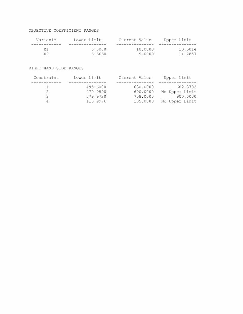
OBJECTIVE COEFFICIENT RANGES

Variable Lower Limit Current Value Upper Limit------------ --------------- --------------- ---------------

X1 6.3000 10.0000 13.5014X2 6.6660 9.0000 14.2857

RIGHT HAND SIDE RANGES

Constraint Lower Limit Current Value Upper Limit------------ --------------- --------------- ---------------

1 495.6000 630.0000 682.37322 479.9890 600.0000 No Upper Limit3 579.9720 708.0000 900.00004 116.9976 135.0000 No Upper Limit


Curtis Hubbard Jr.

MGNT 3185, MW 06:00-07:15p.m.


Using the Management Scientist software, the economic order quantity (EOQ) for the

TyTy Beverage Company is 663.32. This value also reflects the maximum inventory level. When

the quantity of inventory reaches $583.73 the total annual cost is minimized. The total cost is

equivalent to the sum of the annual inventory holding cost ($291.86) and the annual ordering

cost ($291.86). TyTy Georgia Beverage Company has a cycle time of 27.14 days; this is the

number of days before the company has to reorder. The company operates 360 days out of the

year and orders 13.27 times within the operating period. When the on hand inventory drops

below 146.67 the TyTy Beverage Company has to reorder more products. The average inventory

level is half the EOQ and has a value of 331.66.

INVENTORY MODEL***************

ECONOMIC ORDER QUANTITY***********************

YOU HAVE INPUT THE FOLLOWING DATA:**********************************

ANNUAL DEMAND = 3900 UNITS PER YEAR

ORDERING COST = $20 PER ORDER

INVENTORY HOLDING COST:A. ANNUAL INVENTORY CARRYING CHARGE = 11.0%B. COST PER UNIT = $ 4 PER UNIT

WORKING DAYS PER YEAR = 360 DAYS

LEAD TIME FOR A NEW ORDER = 4 DAYS

INVENTORY POLICY****************

OPTIMAL ORDER QUANTITY 595.44

ANNUAL INVENTORY HOLDING COST $131.00

ANNUAL ORDERING COST $131.00

TOTAL ANNUAL COST $261.99

MAXIMUM INVENTORY LEVEL 595.44

AVERAGE INVENTORY LEVEL 297.72

REORDER POINT 43.33

NUMBER OF ORDERS PER YEAR 6.55

CYCLE TIME (DAYS) 54.96


Curtis Hubbard Jr.

MGNT 3185, MW 06:00-07:15p.m.


Using the Management Scientist software, the economic order quantity is 2,500.00; this

is the point that the ordering and holding cost are at their lowest. The annual cost is $31,229.70,

which is the sum of the annual ordering and holding cost. The average inventory level is half of

the optimal order quantity and has a value of 1,250.00. The cycle time is 96.15 days between

orders. When inventory drops to 130.00 the company will order more supplies. The company has

250 working days a year and makes 2.60 orders per year.

INVENTORY MODEL***************

ECONOMIC ORDER QUANTITY WITH QUANTITY DISCOUNTS***********************************************

YOU HAVE INPUT THE FOLLOWING DATA:**********************************

QUANTITY DISCOUNT INFORMATION

CATEGORY UNIT COST MINIMUM QUANTITY-------- --------- ----------------

1 $5.00 02 $4.85 10003 $4.75 2500

ANNUAL DEMAND = 6500 UNITS PER YEAR

ORDERING COST = $47 PER ORDER

ANNUAL INVENTORY CARRYING CHARGE = 21

WORKING DAYS PER YEAR = 250 DAYS

LEAD TIME FOR A NEW ORDER = 5 DAYS

INVENTORY POLICY****************

OPTIMAL ORDER QUANTITY 2,500.00

ANNUAL INVENTORY HOLDING COST $1,246.88

ANNUAL ORDERING COST $122.20

ANNUAL PURCHASE COST $30,875.00

TOTAL ANNUAL COST $32,244.08

MAXIMUM INVENTORY LEVEL 2,500.00

AVERAGE INVENTORY LEVEL 1,250.00

REORDER POINT 130.00

NUMBER OF ORDERS PER YEAR 2.6CYCLE TIME (DAYS) 96.15

production operations management portfolio (p om) … · production operations management portfolio...

Documents