production planning and inventory control with ... · pdf fileproduction planning and...

E L S E V I E R European Journal of Operational Research 102 (1997) 264-278

EUROPEAN JOURNAL

OF OPERATIONAL RESEARCH

Production planning and inventory control with remanufacturing and disposal

Erwin van der Laan*, Marc Salomon /~fdeling Bedrijf*kunde, Erasmus Universiteit Rotterdam, PO. Box 1738, NL-3000 DR Rotterdam, The Netherlands

Abstract

In this paper we consider a stochastic inventory system with production, remanufacturing, and disposal operations. Customer demands must either be fulfilled from the production of new products or by the remanufacturing of used products. Used products are either remanufactured or disposed of. To coordinate production, remanufacturing and disposal operations efficiently, we extend the PUSH and PULL strategies that Van der Laan et al. developed to control a system in which all returned products are remanufactured and no planned disposals occur. The other contributions of this paper are to indicate when and why planned disposals are economically beneficial, and to compare the PUSH-disposal strategy to the PULL- disposal strategy. In addition, we investigate the robustness of the control parameters of the PUSH- and PULL-disposal strategy over the different stages of a product life-cycle. @ 1997 Elsevier Science B.V.

Keywords: Production planning; Inventory control; Manufacturing; Remanufacturing; Disposal; Product life-cycle; Statistical reorder point strategies; Computational experiments

1. Introduct ion

Care for the environment, environmental legisla- tion, corporate image, and economical arguments mo- tivate many companies these days to take responsibil- ity for their products alter customer use (see Thierry et al. [9] ). A popular way of dealing with this responsi- bility is to set up a program for the collection and further processing of used products ( ' re turnables ' ) . Pos- sible options to further process returnables include remanufacturing, repair, recycling and disposal (see [ 9] for further definitions of these options).

The production and inventory system that we consider in this paper is a simplified version of a system that has been implemented successfully at a large Dutch manufacturer of photocopiers. The manufac-

* Fax: +31 10 452 3595; e-mail: [email protected]

turer had developed a new generation of photocopiers consisting of easy-to-disassemble modules. Used copiers are collected at the customer site and trans- ported to a disassembly plant for disassembly into modules. Modules that satisfy certain specific quality requirements are remanufactured in a remanufacturing plant. After remanufacturing modules are considered as 'new', and can in principle be assembled with newly manufactured modules to obtain a copier that is sold in the market for new products. Modules that do not satisfy the quality standards for remanufacturing are either used as spare-parts for the second-hand market or disposed of.

Although the system implemented at the copier manufacturer may be ecologically sound due to module remanufacturing and material reuse, production and inventories are more difficult to plan and control

0377-2217/97/$17.00 (~) 1997 Elsevier Science B.V. All rights reserved. PII S0377-22 17 (97)00108-2

E. van der Laan. M. Salomon/European Journal of Operational Research 102 (1997) 264-278 265

than in traditional systems without remanufacturing. It has been experienced that these difficulties are mainly due to the many interactions that exist between the manufacturing, remanufacturing and disposal operations. Interactions between manufacturing and remanufacturing processes occur for instance when the output of the remanufacturing process is too low to satisfy all the demands for new modules adequately. In this case manufacturing orders must be placed regularly to avoid shortages.

To plan and control manufacturing, remanufacturing, and disposal operations simultaneously, the copier remanufacturer implemented a PUSH strategy. By this strategy returned modules are 'pushed' through the remanufacturing process as soon as a sufficient amount of modules becomes available from the disassembly plant. If the joint inventory of new and remanufactured modules appears to be too low to satisfy the future expected demands adequately, a manufacturing order is placed to produce new modules. In principle, disposal of a disassembled module occurs only when the quality of the module is insufficient for remanufacturing.

The copier manufacturer had the impression that the efficiency of their system could be improved by the introduction of a control strategy which offers a higher level of coordination between the manufacturing, remanufacturing and disposal operations. For this purpose, the change to a PULL strategy had been investigated. Under this strategy disassembled modules are 'pulled' through the remanufacturing process only when they are actually needed to satisfy the demand tot new modules. If the output of the remanufacturing process appears to be too low to cover the future expected demands, a manufacturing order is placed.

Interactions between remanufacturing and disposal processes occur when the number of returned modules is higher than the demand for new modules. In this case some of the returned modules must be disposed of instead of being remanufactured to avoid too high, and therefore too expensive, stocking positions. Therefore, another way that had been considered to improve the system efficiency is to not only dispose of returned products when their quality is too low for remanufacturing, but also when the system inventories become too high.

This paper is on production planning and inventory control tor systems in which careful coordination between manufacturing, remanufacturing and disposal

operations is essential for achieving maximum system efficiency. In the production planning and inventory control literature numerous periodic review and continuous review strategies have been proposed that apply to similar systems as the one defined above. For an extensive overview we refer to Van der Laan et al. [3]. In the brief overview below we restrict ourselves to the class of continuous review strategies, since the strategies that we consider in this paper also belong to this class.

The first to consider a continuous review strategy for a production/inventory system with remanufacturing and disposal has been Heyman [ 1 ]. Although the strategy in [ 1 ] is optimal (i.e., no alternative strategy exists that yields lower total expected costs), it applies only to systems without fixed costs and with zero lead times. The model that Muckstadt and Isaac [ 7 ] developed differs from Heyman's in the sense that they allow for non-zero manufacturing lead times, stochastic remanufacturing lead times, and finite remanufacturing capacity. Disposal operations are not considered and the procedure to find the optimal decision parameters is approximative. Van der Laan et al. [5] extend the work of Heyman, by formulating a PUSH strategy that applies to systems with non-zero fixed manufacturing costs, non-zero manufacturing lead times, and stochastic remanufacturing lead times. Limitations of [5] are however that the demands and returns are modelled by uncorrelated Poisson processes, and that holding costs of remanufacturables are zero. Further- more, the procedure to calculate the total expected costs is approximative rather than exact. In a follow- up paper Van der Laan et al. [4] consider a system with non-zero holding costs for remanufacturables. To control this system, [4] suggests two PUSH-strategies and presents an exact procedure to calculate the total expected costs. In [3] a PUSH and PULL strategy is formulated for a similar system that allows for correlation and Coxian-2 distributed return and demand flows. Van der Laan et al. [6] extend this model to allow for discrete lead time distributions. Both papers however do not consider disposal operations. Recently, an optimal EOQ-like policy for a deterministic system with manufacturing, repair, and disposal operations and zero lead times has been proposed by Richter [ 8 ].

The contributions of this paper are as follows. First, we formulate a general manufacturing/remanufacturing system with disposal operations,

266 E. van der Laan, M. Salomon/European Journal of Operational Research 102 (1997) 264-278

Returned products

Remanufacturable inventory

= Planned disposals

Remanufacturing i I Manufacturing 1 Y

Serviceable inventory

[ = Demanded new products

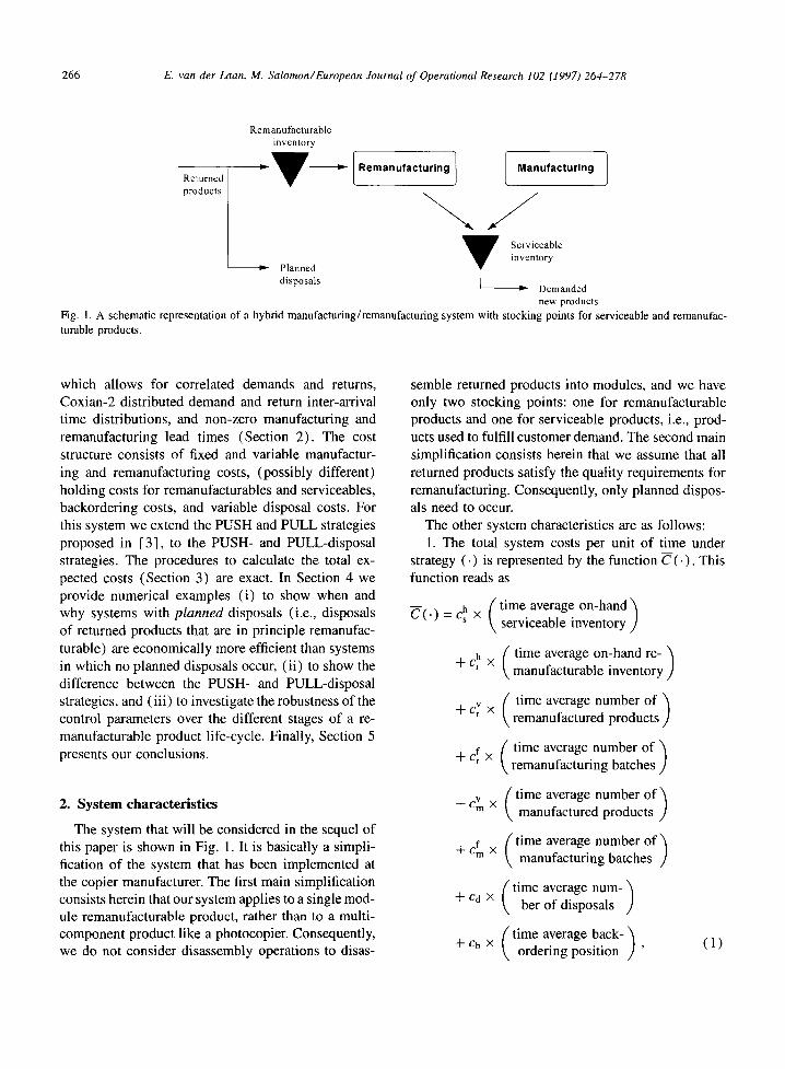
Fig. 1. A schematic representation of a hybrid manufacturing/remanufacturing system with stocking points for serviceable and remanufacturable products.

which allows for correlated demands and returns, Coxian-2 distributed demand and return inter-arrival time distributions, and non-zero manufacturing and remanufacturing lead times (Section 2). The cost structure consists of fixed and variable manufacturing and remanufacturing costs, (possibly different) holding costs for remanufacturables and serviceables, backordering costs, and variable disposal costs. For this system we extend the PUSH and PULL strategies proposed in [3], to the PUSH- and PULL-disposal strategies. The procedures to calculate the total expected costs (Section 3) are exact. In Section 4 we provide numerical examples (i) to show when and why systems with planned disposals (i.e., disposals of returned products that are in principle remanufacturable) are economically more efficient than systems in which no planned disposals occur, (ii) to show the difference between the PUSH- and PULL-disposal strategies, and (iii) to investigate the robustness of the control parameters over the different stages of a remanufacturable product life-cycle. Finally, Section 5 presents our conclusions.

2. S y s t e m c h a r a c t e r i s t i c s

The system that will be considered in the sequel of this paper is shown in Fig. 1. It is basically a simplification of the system that has been implemented at the copier manufacturer. The first main simplification consists herein that our system applies to a single module remanufacturable product, rather than to a multi- component product like a photocopier. Consequently, we do not consider disassembly operations to disas-

semble returned products into modules, and we have only two stocking points: one for remanufacturable products and one for serviceable products, i.e., products used to fulfill customer demand. The second main simplification consists herein that we assume that all returned products satisfy the quality requirements for remanufacturing. Consequently, only planned disposals need to occur.

The other system characteristics are as follows: 1. The total system costs per unit of time under

strategy (.) is represented by the function C-(. ). This function reads as

- - h ( time average on-hand "~ C (.) = c s x serviceable inventory /

h time average on-hand re- ) + c r x manufacturable inventory

/

time average number of ) + c v x remanufactured products

/

f ( time average number of ) + c r x remanufacturing batches

/' time average number of + c v x \ manufactured products ]

f /" time average number of + c m x \ manufacturing batches ,]

//time average num- ) + Cd X \ ber of disposals

/" time average back- "~ + Cb × \ ordering position J ' (1)

E. van der Laan, M. Salomon/European Journal of Operational Research 102 (1997) 264-278

where c~ ' are the inventory holding costs per product in serviceable inventory per unit of time, c~ are the inventory holding costs per product in remanufacturable

v inventory per unit of time, c m are the variable reman-

ufacturing costs per product, c~ are the fixed remanufacturing costs per batch, C~n are the variable manufacturing costs per product (including material costs),

f Cm are the fixed manufacturing costs per batch, Cd are the disposal costs per product, and Cb are the backordering costs per product per unit of time. All cost factors are non-negative, except the disposal costs ca, which are negative when the returned products have a positive salvage value.

2. The inter-occurrence times between two successive demands for new products and two successive returns of used products are Coxian-2 distributed (see Appendix A). The demand rate is ,~D and the return rate is AR. The uncertainties in demand and return processes are reflected by the squared coefficients of variation cv~ for the demands and cv 2 for the returns. The correlation between demands and returns is modelled by the coefficient p, which is the probability that a product return instantaneously generates a product demand.

3. Demands that cannot be fulfilled immediately are backordered.

4. The manufacturing lead time Lm and the remanufacturing lead time Lr are constant.

In the next section we formulate the PUSH- and PULL-disposal strategy, that will be used to control the system above,

3. Strategy definit ions and analys is

As an extension to the PUSH and PULL strategy that have been considered in [3] (which do not consider disposal operations), we define the PUSH- disposal and PULL-disposal strategy as follows:

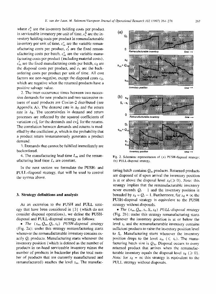
• The (sin, Qm, Qr, Sd) PUSH-disposal strategy (Fig. 2a): under this strategy remanufacturing starts whenever the remanufacturable inventory contains ex- actly Qr products. Manufacturing starts whenever the inventory position (which is defined as the number of products in on-hand serviceable inventory minus the number of products in backorder plus the total number of products that are currently manufactured and remanufactured) reaches the level sin. The manufac-

267

Q r .e [ ~ . . . . . . . . . . . . .

o Remsnufacturable inventory time

S m + a m f ~ ~ .:~..:~

• ,N q~ Sm

Inventory position time --~

(b) Sd ~ ; ~ ~ % ~

0 Remanufactursble inventory time . - *

Or ~ ~ ~ % ~ :

:r m

Inventory position time ---~

Fig. 2. Schematic representation of (a) PUSH-disposal strategy; (b) PULL-disposal strategy.

turing batch contains Qm products. Returned products are disposed of if upon arrival the inventory position is at or above the disposal level sa(~> 0). Note: this strategy implies that the remanufacturable inventory never exceeds Qr - 1 and the inventory position is

bounded by s d + Qr - 1. Furthermore, for sa = pc the PUSH-disposal strategy is equivalent to the PUSH strategy without disposals.

• The (sin, Qm, Sr, St, sd) PULL-disposal strategy (Fig. 2b): under this strategy remanufacturing starts whenever the inventory position is at or below the level Sr and the remanufacturable inventory contains sufficient products to raise the inventory position level to St. Manufacturing starts whenever the inventory position drops to the level Sm (~< st). The manufacturing batch size is Qm. Disposal occurs to every returned product that arrives when the remanufacturable inventory equals the disposal level Sd (~> 0). Note: for sa = pc this strategy is equivalent to the PULL strategy without disposals.

268

Table l Notation

E. van der Laan. M. Sa lomon/European Journal o f Operational Research 102 (1997) 264 -278

l~Ct(t)

I s ( t )

t,gn(O

D ( t o , tl )

Enet(t - to, t - tl )

-OH lr

Lmin

Lmax

= The net serviceable inventory at time t, defined as the number of products in on-hand serviceable inventory minus the number of products in backorder at time t

= The serviceable inventory position at time t, defined as the net serviceable inventory plus the number of products in manufacturing work-in-process plus the number of products in remanufacturing work-in-process

= The number of products in remanufacturable on-hand inventory at time t

= The demands in the time-interval (to, tl ]

= The number of products planned to be manufactured and remanufactured in the time-interval ( t - to, t - tl I

that enter serviceable inventory at or before time t minus the demands in the interval ( t - to, t - tl ]

= The time-average backordering position

= The time-average on-hand serviceable inventory

= The time-average on-hand remanufacturable inventory

= The time-average number of remanufacturing orders

= The minimum of the manufacturing and remanufacturing lead time

-- The maximum of the manufacturing and remanufacturing lead time

Remark. Alternatively to this PULL-disposal strategy we have also investigated a variant with a fixed remanufacturing batch size. Numerical experiments showed that the difference between the two strategies is however small. Therefore, we restrict the discus- sion in this paper to the above implementation.

As can be concluded from the above, the most im- portant difference between PUSH and PULL control is the timing of remanufacturing and disposal operations. With PUSH control the start of the remanufacturing operation is solely based on the number of products in remanufacturable inventory, whereas under PULL control the start depends both on the inventory position and on the number of products in remanufacturable inventory. Furthermore, under the PUSH-disposal strategy the disposal decision depends on the inventory position, whereas it depends under the PULL-disposal strategy on the on-hand remanufacturable inventory. The reason why in these two strategies the disposal decision is based on different inventories is that under PUSH control without planned disposals the inventory position (and therefore the serviceable inventory) is unbounded, i.e. may grow uncontrollably high, whereas under PULL control without planned disposals the remanufacturable inventory is unbounded. By defining Sd the way we did for the PUSH- and PULL- disposal strategy, all inventories are controllable.

In Section 3.1 and Section 3.2 we outline a procedure to calculate the total expected costs (1) for the PUSH- and PULL-disposal strategy respectively. The notation that we use in this outline is specified in Ta- ble 1. For ease of explanation we have restricted the scope of the outline to the situation with uncorrelated and exponentially distributed demand and return inter- occurrence times. For the modifications required to model correlations and Coxian-2 distributed demand and return inter-occurrence times we refer to Van der Laan et al. [ 3].

To find

C-;OSH-d = min C-(sm, Qm, Qr, Sd),

the minimal system costs under PUSH-disposal control, and

C ; U L L - d = min C-( Sm, Q m , Sr, Sr , Sd ) ,

the minimal system costs under PULL-disposal control, we implemented an enumerative search procedure.

3.1. Analysis of the (sin, Qm, Qr, so) PUSH-disposal strategy

The state transitions of the manufacturing/remanufacturing system defined in Section 2 under the PUSH- disposal strategy can be formulated as a continuous

E. van der Laan, M. Sa lomon/European Journal o f Operational Research 102 (1997) 264-278 269

time Markov chain. This Markov chain, 3,41 say, has two-dimensional state variable

Xl(t) = {Is(t),IrOH(t) I t > 0} and a two-dimensional state space

$, = { s , n -+- 1 . . . . . U , } x { 0 . . . . . Q r - 1 } ,

where UI = max {Sd + Q~ - 1, Sm + Qm}. The transition rate v,,,,,s,'-, related to a transition from state s (j) ~ 8~ to s (2) E $I is defined in Table 2.

The limiting joint probability distribution

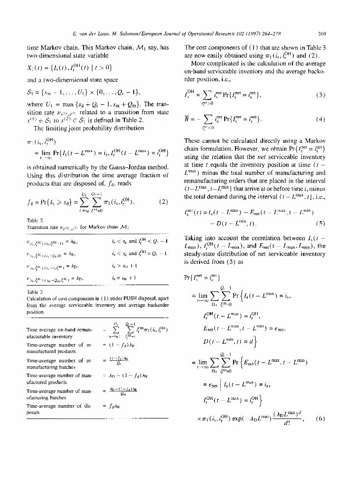
The cost components of ( 1 ) that are shown in Table 3 are now easily obtained using 7rl (is,/OH) and (2).

More complicated is the calculation of the average on-hand serviceable inventory and the average backorder position, i.e.,

•OH Z ts P r { l s _ .net~ s .net net = - t s j~, (3) U'>0

-- Z .net pr,rlnet /net} B = - ts L s = , . ( 4 )

?,'~' <0

"n'l ( is, i OH )

= lim Pr{Is( t - L ma×) = i s , l O H ( t -- L ma~) =/OH} t ~ O < >

is obtained numerically by the Gauss-Jordan method. Using this distribution the time average fraction of products that are disposed of, fd, reads

UI Q r - 1

fd = Pr{Is ~> Sd}= Z Z "rrl(is'iOH)" (2) i~=so tim=0

Table 2 Transition rate Vs~j~¢?~ for Markov chain .Adl

V(is,/r)ll ) , ( i s , i ( r ) l l+ l ) = A R ,

Plis,i~ )11 ) ,( is t-Qr,O) = /~R,

P(is./r Ill ),(is - I,i~ )11 ) -- ~-D,

P (is,i~lll ),( %n +Qm,t~t)II ) = "~D,

is < so and tr ~H < Q r - 1

is < Sd and t~ H = Q , - - 1

is > Sm + 1

is = Sm + 1

Table 3 Calculation of cost components in ( 1 ) under PUSH disposal, apart from the average serviceable inventory and average backorder position

UI Q,- 1

Time-average on-hand reman- = ~ ~ l~H~rl (is, t<r )H) ufacturable inventory is=sm+l t~)tl=l Time-average number of re- = ( 1 - fd)AR manufactured products

Time-average number of re- - (l-'t'~gaR -- Qr

manufacturing batches

Time-average number of man- = AD -- ( 1 -- fd) AR ufactured products

Time-average number of man- - AD--(I--fd)AR -- Qm

ufacturing batches

Time-average number of dis- = fdAR posals

These cannot be calculated directly using a Markov chain formulation. However, we obtain Pr{l net =/net}

using the relation that the n e t serviceable inventory at time t equals the inventory position at time (t - L max) minus the total number of manufacturing and remanufacturing orders that are placed in the interval ( t - L max , t - L rain ] that arrive at or before time t, minus the total demand during the interval (t - L m~X, t], i.e.,

/net(t) = l s ( t - L max) + E n e t ( t - L max, t - L rain)

- D ( t - L rain, t). (5)

Taking into account the correlation between Is (t - Lmax), I O H ( t -- Lmax), and Ene t ( t - Lmax, Lmin) , the steady-state distribution of net serviceable inventory is derived from (5) as

Pr{inet =/net}

Qr- 1

= l i m

fh t~m=0

1 O H ( t - L max) = i?H,

Enet ( t L max , t L min ) -- -- = enet,

D ( t - L rain, t) = d}

Q,-1

= l i m Z Z P r {

nL ~)m=0

= enet Is (t - L max) = is,

l ? H ( t _ Lma×) = i ? H }

×'rrl (is,/OH) exp( --AD Lmin) ( I D L m i n ) d d! '

(6)

270

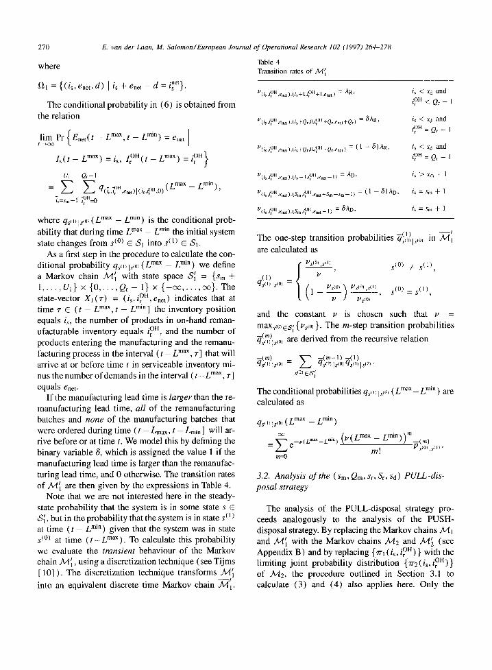
where

~1 = {( i s , enet ,d) I is + e , e t _ d = inet}.

The conditional probability in (6) is obtained from the relation

E. van der Laan, M. Salomon/European Journal o f Operational Research 102 (1997) 264-278

Table 4

Transi t ion rates o f .Mti

P(is,tOrlt enet),(is+l,t?ll +l,enet) = AR,

(ts,t r ,ene ),Os+Qr,O,t r +Qr,ene + Q r )

is < s d and ~,*?" < Q r - I

is < sd and

lim Pr {Enet(t L max, t L min) - - - - = enet l ----~ OO

l s ( t - L max) = is, IrOH(t - L max) = /OH}

Ut Qr - 1

= ~ - ' ~ Z q .= ~o. g max _ L min) ~ t~,t~ ,e,~t ) l ( i~,t~)",O ) (

v. ~ • ~ = (1 - 8).~R, (ts,t r ,ene ) ,( ts+Qr,0,1r +Qr,enc )

/d . OH • -011 = ~-D, (/s,t r , ene t ) , ( t s - - l , t r , ene t - - I )

v • ~). ~)ll = ( I -- 3 )a t9 , (Is,It ,enel ),~ Sm ,t r , e n e l + S m - - s m - - l )

.v . ~ t t ~ )H = ~ / ~ D , (ts,t r ,enel),(Sm,t r , ene l - - l )

t~ )H = Q,. - 1

is < so and

t~ H = Or - 1

i s > s m + l

i s = s m + l

is = S m + 1

where qs, , Is ,0, ( Lmax - Lmin) is the conditional probability that during time L max - - L min the initial system state changes from s (°) C $1 into s (1) E SI.

As a first step in the procedure to calculate the conditional probability qs~,ls~O~ ( L m a x - - Lmin) we define a Markov chain .A~] with state space $~ = {sin + 1 . . . . . Vl} × {0 . . . . . Qr - 1} × { - 0 0 . . . . . 00}. The state-vector Xl (7-) = (is, iro H, enet) indicates that at time 7- E ( t - L max, t - L min ] the inventory position equals i~, the number of products in on-hand remanufacturable inventory equals iro H, and the number of products entering the manufacturing and the remanufacturing process in the interval (t - L max , 7"] that will arrive at or before time t in serviceable inventory minus the number of demands in the interval ( t - L max, 7"] equals ene t.

If the manufacturing lead time is larger than the remanufacturing lead time, all of the remanufacturing batches and none of the manufacturing batches that were ordered during time ( t - L m a x , t - Lmin ] will arrive before or at t ime r We model this by defining the binary variable 6, which is assigned the value 1 if the manufacturing lead time is larger than the remanufacturing lead time, and 0 otherwise. The transition rates of ./kd~ are then given by the expressions in Table 4.

Note that we are not interested here in the steady- state probabili ty that the system is in some state s C S~, but in the probability that the system is in state s (1) at time (t - - L ra in) given that the system was in state s ~°) at time ( t - L max). To calculate this probability we evaluate the t ransient behaviour of the Markov chain ./L4~1, using a discretization technique (see Tijms [10] ) . The discretization technique transforms .A//~

into an equivalent discrete time Markov chain M~I.

The one-step transition probabilities -~qs.,t) Is,O, in ~ ' l are calculated as

{ r l.'slOl,s~l~ S(0) =/= S(1)

= ( 1 ) /"

qs(I)[ s(°l = ( Psl0~ Vs~Ol ~¢1~ l - - " , s ( ° ) = s ( l ) ,

• ~ 11 PS(0)

and the constant v ts chosen such that v = maxs~o~6s ( {vs~o~ }. The m-step transition probabilities

s'" Is~0~ are derived from the recursive relation

- - (m) ~ ( m - 1) ~ ( 1 ) qs'~ls ~°~ = Z %~Z~ls~°~'~s~"ls~2~"

s 12) ES~

The conditional probabilities q,~"~ I,~°~ ( L max - - L rain ) are calculated as

qs, i Isl01 ( L max - L min )

o o = Z e__V(trnax_tmin ) ( / - I ( t m a x - t m i n ) ) m _ ~ ( m ) m! Fs~O~,s,~ •

m--O

3.2. Analys is o f the (Sm, Qm, Sr, St, sa) PULL-d i s - posa l strategy

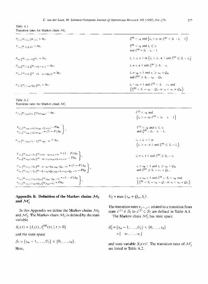
The analysis of the PULL-disposal strategy pro- ceeds analogously to the analysis of the PUSH- disposal strategy. By replacing the Markov chains .M I and A,'[~ with the Markov chains .AA2 and .M~ (see Appendix B) and by replacing {zrl (it, ir °n) } with the limiting joint probability distribution {zr2 (i~, i °n ) } of .AA2, the procedure outlined in Section 3.1 to calculate (3) and (4) also applies here. Only the

E. van der Laan, M. Salomon/European Journal of Operational Research 102 (1997) 264-278

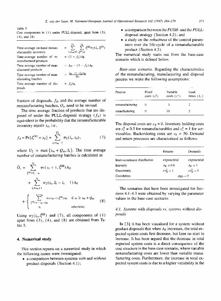
Table 5 Cost components in (1) under PULL-disposal, apart from (3), (4), and (8)

U2 Sd

Time-average on-hand reman- = ~ 2 /'()Hq-/-,. 2ts,'i t~. H'r ) ufacturable inventory is=sm+l r~II=l Time-average number of re- = ( 1 - fd)Ar manufactured products Time-average number of man- = AD -- ( 1 - f d ) AR ufactured products Time-average number of man- - ao-(l-f'0a~

- - Qm ufacturing batches Time-average number of dis- = fdAr posals

fraction of disposals, fd, and the average number of remanufacturing batches, Or, need to be revised.

The time average fraction of products that are disposed of under the PULL-disposal strategy ( fd ) is equivalent to the probabi l i ty that the remanufacturable

inventory equals Sd, i.e.,

U2

f d : P r { l O H = s d } = Z ~2( is ,Sd) , (7) is=Sm+l

where U2 = max {Sm + Qm, St}. The time average number of remanufacturing batches is calculated as

.'¢d

Or = ~ ~r2(sr+ I,iOH)aD

Sr

+ Z 7"r2(is, S r - i s - l ) a R is = Sm + I

sr -- qn 7r2(Sm+l,lrOH).~W i f Sr /> S m + Qm,

-q- ,~m=s~ . . . . -Ore

O, o the rw i se .

(8)

Using 7"r2(is, i OH) and (7 ) , all components of (1) apart from (3) , (4 ) , and (8) are obtained from Ta-

ble 5.

4. Numerical study

This section reports on a numerical study in which the fol lowing issues were investigated:

• a comparison between systems with and without product disposals (Section 4.1 ) ;

271

• a comparison between the PUSH- and the PULL- disposal strategy (Section 4.2) ; and

• a study on the robustness of the control parameters over the l ife-cycle of a remanufacturable product (Section 4.3).

The numerical study starts out from the base-case scenario which is defined below.

Base-case scenario. Regarding the characteristics of the remanufacturing, manufacturing and disposal process we make the following assumptions:

Process Fixed Variable Lead costs (c f) costs (c v) times (L.)

remanufacturing 0 5 2

manufacturing 0 10 2

The disposal costs are Cd = 0. Inventory holding costs are c~ = 0.5 for remanufacturables and c~ = 1 for serviceables. Backordering costs are Cb = 50. Demand and return processes are characterized as follows:

Returns Demands

Inter-occurrence distribution exponential exponential

Intensity ,~R = 0.8 AD = 1 Uncertainty cv 2 = 1 cv~ = 1

Corre la t ion PRD = 0

The scenarios that have been investigated for Sec- tions 4.1-4.3 were obtained by varying the parameter values in the base-case scenario.

4.1. Systems with disposals vs. systems without disposals

In [3] it has been visualised for a system without product disposals that when AR increases, the total expected system costs first decrease, but later on start to increase. It has been argued that the decrease in total expected system costs is a direct consequence of the cost structure in the base-case scenario, where variable remanufacturing costs are lower than variable manufacturing costs. Furthermore, the increase in total expected system costs is due to a higher variabili ty in the


Costs

C'PUSH_ d 16

14 . . . . . . ~ _

(a) 10 i i

000 0.15 0.30 0.45 0.60 ' 0.75 2 R - -~

/ /

i

0.90

Costs

18

+ ~PULLId J 16

(b) 10 i i , i •

0.00 0.15 0.30 0.45 0.60 0.75 0.90

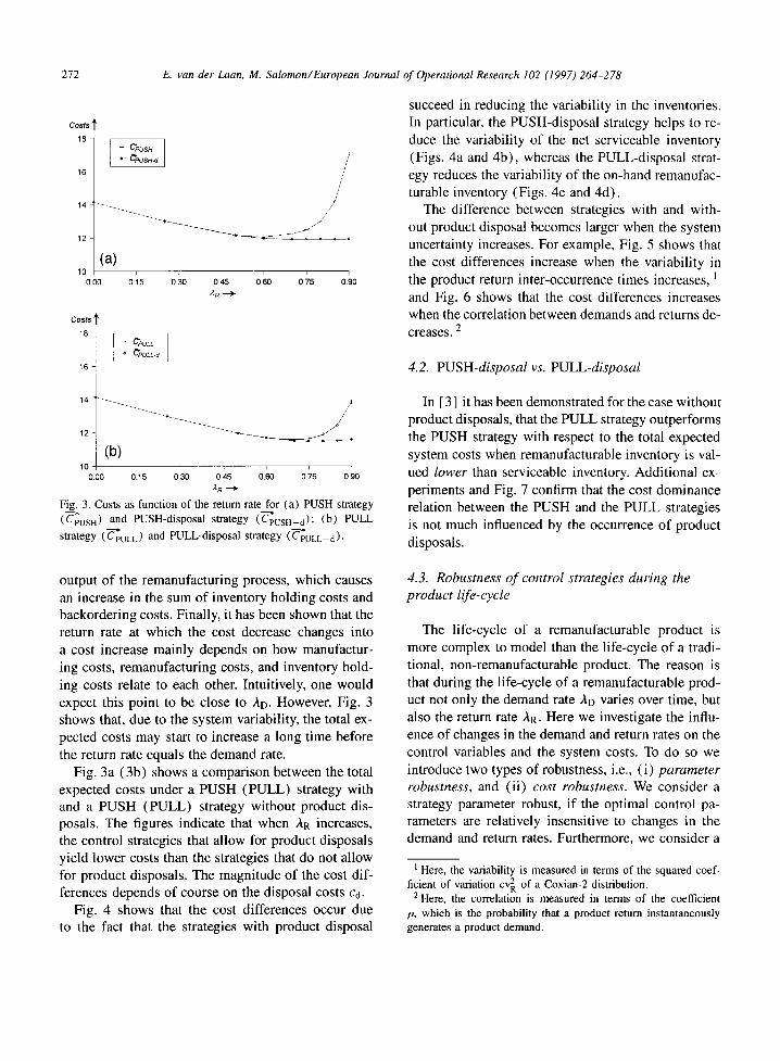
Fig. 3. Costs as function of the return rate for (a) PUSH strategy (C-;uSH) and PUSH-disposal strategy (~PUSH--d); (b) PULL strategy (C~uLL) and PULL-disposal strategy (~ULL--d).

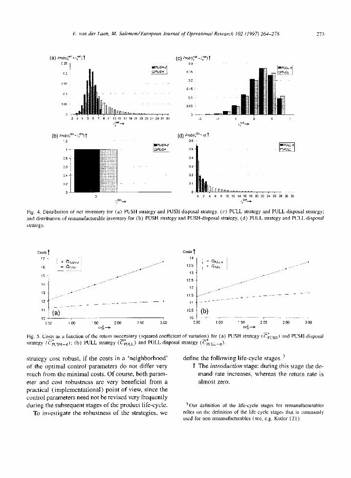
succeed in reducing the variability in the inventories. In particular, the PUSH-disposal strategy helps to re- duce the variability of the net serviceable inventory (Figs. 4a and 4b), whereas the PULL-disposal strategy reduces the variability of the on-hand remanufacturable inventory (Figs. 4c and 4d).

The difference between strategies with and without product disposal becomes larger when the system uncertainty increases. For example, Fig. 5 shows that the cost differences increase when the variability in the product return inter-occurrence times increases, ] and Fig. 6 shows that the cost differences increases when the correlation between demands and returns de-

2 creases.

4.2. PUSH-disposal vs. PULL-disposal

In [ 3 ] it has been demonstrated for the case without product disposals, that the PULL strategy outperforms the PUSH strategy with respect to the total expected system costs when remanufacturable inventory is valued lower than serviceable inventory. Additional experiments and Fig. 7 confirm that the cost dominance relation between the PUSH and the PULL strategies is not much influenced by the occurrence of product disposals.

output of the remanufacturing process, which causes an increase in the sum of inventory holding costs and backordering costs. Finally, it has been shown that the return rate at which the cost decrease changes into a cost increase mainly depends on how manufacturing costs, remanufacturing costs, and inventory holding costs relate to each other. Intuitively, one would expect this point to be close to At). However, Fig. 3 shows that, due to the system variability, the total expected costs may start to increase a long time before the return rate equals the demand rate.

Fig. 3a (3b) shows a comparison between the total expected costs under a PUSH (PULL) strategy with and a PUSH (PULL) strategy without product disposals. The figures indicate that when AR increases, the control strategies that allow for product disposals yield lower costs than the strategies that do not allow for product disposals. The magnitude of the cost differences depends of course on the disposal costs ca.

Fig. 4 shows that the cost differences occur due to the fact that the strategies with product disposal

4.3. Robustness o f control strategies during the product life-cycle

The life-cycle of a remanufacturable product is more complex to model than the life-cycle of a traditional, non-remanufacturable product. The reason is that during the life-cycle of a remanufacturable product not only the demand rate ,h. D varies over time, but also the return rate -~R. Here we investigate the influ- ence of changes in the demand and return rates on the control variables and the system costs. To do so we introduce two types of robustness, i.e., (i) parameter robustness, and (ii) cost robustness. We consider a strategy parameter robust, if the optimal control parameters are relatively insensitive to changes in the demand and return rates. Furthermore, we consider a

I Here, the variability is measured in terms of the squared coefficient of variation cv 2 of a Coxian-2 distribution.

2 Here, the correlation is measured in terms of the coefficient p, which is the probability that a product return instantaneously generates a product demand.

E, van der Laan, M. Salomon/European Journal of Operational Research 102 (1997) 264-278 273

(a) Prob~2 et= iff or} f

0 25 1

0 1 5

0 0 5

0 n _

-3 -1 1 3

(b) mob(l~ ° ' : #o.} t 12

1

08

06

04

0.2

O

5 7 9 11 13 15 17 19 21 23 25 27 29 31 33 i ne t . .~

ioH.._.

(c) P~ob(¢ ~': ¢°') t 03

025

02

015

01

005

0 , -3

(d) Pr°b{ I° '= ~) t 06

05

04

03

02

01

0

i i i

-1 1 3 7

i snet.-~

; . . . . . .

2 4 6 8 10 12 14 16 18 20 22 24 26 28 30 32 irOH..--~

Fig. 4. Distribution of net inventory for (a) PUSH strategy and PUSH-disposal strategy, (c) PULL strategy and PULL-disposal strategy; and distribution of remanufacturable inventory for (b) PUSH strategy and PUSH-disposal strategy, (d) PULL strategy and PULL-disposal strategy.

Costs

17 + ~PUSH-d ] 16 + ~PUSH l, 15

14 ~ , ~ j _ J -

13 s - ~ - - - -

12

" (a) 10 i i

0.50 1 O0 1 5 0

z J - j _ . - -

j j ~ J

' o 2.00 2.50 3. 0

Costs ' 14

C*PULL-d 13.5 + ~putc .... ~ - I - ~

1 2 5 ~ ' - ~ - . . . .

12 ~ , , J

11.5 J f . . . . - - . . . . . .

10.5 ( b )

lO 0.50 1.00 ~ .50 2.0o 2.50 3.00

ov,~.-~

Fig. 5. Costs as a function of the retum uncertainty (squared coefficient of variation) for (a) PUSH strategy (C'~'USH) and PUSH-disposal strategy ( PUSH-d); (b) PULL strategy (CpuLL) and PULL-disposal strategy (C-~'ULL--O)-

strategy cost robust, i f the costs in a 'neighborhood' of the optimal control parameters do not differ very much from the minimal costs. Of course, both parameter and cost robustness are very beneficial from a practical ( implementat iona l ) point o f view, since the control parameters need not be revised very frequently during the subsequent stages o f the product l i fe-cycle.

To investigate the robustness of the strategies, we

define the fo l lowing l i fe-cycle stages. 3 I The introduction stage: during this stage the de-

mand rate increases, whereas the return rate is almost zero.

3 Our definition of the life-cycle stages for remanufacturables relies on the definition of the life-cycle stages that is commonly used for non-remanufacturables (see, e.g. Kotler [ 21 ).


Costs ! Costs

135 - ~ 12 " ~ " ~ ~ ~PULL 13 ~ " ~ - ~

--.... ~ 12

11 ~ ~ - . . ~ _ ~ ~ 10.5

lO.S (a) (b) "~- 10 , , ~ ~ , 10 , , , ,

0.00 0.20 0,40 0.60 0.80 1.00 0.00 0.20 0.40 0.60 0,80 1.00 pRo--~ pR~

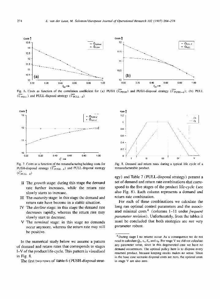
Fig. 6. Costs as function of the correlation coefficient for (a) PUSH (C-~uSH) and PUSH-disposal strategy (~USH-d); (b) PULL (C-PuLL) and PULL-disposal strategy (C-PuLL--d) '

Costs

13

12

10 0.00 0.20

SH---d~ LL-d|

, . ~

0~o 060 080 ,00

Fig. 7. Costs as a function of the renanufacturing holding costs for PUSH-disposal strategy ( ~ U S H - J ) and PULL-disposal strategy

( PULL--d)"

II The growth stage: during this stage the demand rate further increases, while the return rate slowly starts to increase.

III The maturity stage: in this stage the demand and return rate have become in a stable situation.

IV The decline stage: in this stage the demand rate decreases rapidly, whereas the return rate may slowly start to decrease.

V The terminal stage: in this stage no demands occur anymore, whereas the return rate may still be positive.

In the numerical study below we assume a pattern of demand and return rates that corresponds to stages I-V of the product life-cycle. This pattern is visualised in Fig. 8.

The first two rows of Table 6 (PUSH-disposal strat-

Rate

1.2

1

0.8

0.6

0.4

0.2 ~

0

- - Z D

// : \\ ~\ : / / / i ~ " \,

\ i \ \ \ //" \\\ / J \ ; "~

I I I I I I I V V

Fig. 8. Demand and return rates during a typical life cycle of a remanufacturable product.

egy) and Table 7 (PULL-disposal strategy) present a set of demand and return rate combinations that corre- spond to the five stages of the product life-cycle (see also Fig. 8). Each column represents a demand and return rate combination.

For each of these combinations we calculate the long run optimal control parameters and the associated minimal costs 4 (columns 1-11 under frequent parameter revision). Unfortunately, from the tables it must be concluded that both strategies are not very parameter robust.

4 During stage l no returns occur. As a consequence we do not need to calculate Qr, St, St, and Sd. For stage V we did not calculate any parameter value, since in this degenerated case we have no demand occurrences. The optimal policy here is to dispose every returned product, because keeping stocks makes no sense. Since in the base case scenario disposal costs are zero, the optimal costs in stage V are also zero.

E. van de r Laan, M. S a l o m o n / E u r o p e a n Journa l o f Opera t iona l Research 102 (1997) 2 6 4 - 2 7 8

Table 6 Cost comparison between (a) frequent parameter revision of the PUSH-disposal strategy and (b) fixed parameters

275

Stage I Stage I1 Stage lIl Stage IV Introduction Growth Maturity Decline

Stage V Terminal

I 2 3 4 5 6 7 8 9 10 II

AD 0.25 0.50 0.75 1.00 1.00 1.00 0.75 0.50 0.25 0 0 ,~ 0 0 0.20 0.40 0.60 0.80 0.80 0.80 0.60 0.40 0.20

(a ) . f?equent p a r a m e t e r revis ion:

Sm 1 2 3 4 4 4 3 2 t Qm I 1 1 1 1 1 1 I I Qr 1 1 1 1 1 1 1 S d 8 9 8 8 6 5 3

Cr~USH _ d 4.83 8.19 10.32 12.42 11.83 11.41 8.96 6.60 4.14

(b) f i x e d p a r a m e t e r s :

(Sm, Qm, Qr, Sd) C (Sm, Qm, Qr, Sd )

0 0

( I , 1 ,1 ,3) 4.83 11.29 19.70 31.75 29.92 28.50 15.88 7.84 4.14 3.00 3.00 (3, 1, 1,8) 6.01 8.22 10.32 13.28 12.26 11.53 9.32 8.54 8.12 8.00 8.00 (4, 1, 1,8) 7.00 9.04 10.58 12.43 11.83 11.41 9.76 8.83 8.21 8.00 8.00

Table 7 Cost comparison between (a) frequent parameter revision of the PULL-disposal strategy and (b) fixed parameters

Stage I Stage II Stage I11 Stage IV Stage V Introduction Growth Maturity Decline Terminal 1 2 3 4 5 6 7 8 9 10 II

At) 0.25 0.50 0.75 1.00 1.00 1.00 0.75 0.50 0.25 0 0 '~R 0 0 0.20 0.40 0.60 0.80 0.80 0.80 0.60 0.40 0.20

(a) f i ' equen t p a r a m e t e r revis ion:

Sm l 2 3 4 4 4 3 2 1 -

Qm 1 1 1 1 1 1 1 1 1 -

s~. - 4 5 5 5 4 3 2 - -

S,. - 5 6 6 6 5 4 3 -

Sd - 5 6 4 3 2 1 1

Cr~b, Lk_d 4.83 8.19 10.29 12.34 11.65 11.17 8.78 6.45 4.27 0 0

(b) f i x e d p a r a m e t e r s :

( sin, Qm, s,., S,., s o ) C (Sin, Qm, St, Sr, Sd ) ( 1,1,2, 3, l ) 4.83 1 1.29 19.20 30.30 27.66 25.65 13.91 7.02 4.27 3.50 3.50 (3, 1 ,4 ,5 ,5 ) 6.01 8.22 10.29 13.29 12.25 11.54 9.15 8.39 7.90 7.50 7.50 (4, 1 ,5 ,6 ,3 ) 7.00 9.04 10.54 12.35 11.66 11.17 9.48 8.56 7.94 7.50 7.50

Next, we investigate the effects on system costs if we would not regularly revise the control parameters, but fix the control parameters during the complete life- cycle. To this end we take three distinct return and demand rate combinations corresponding to the life- cycle stages represented by the columns 3, 6, and 9.

For each fixed policy (see the first column under fixed parameters) we calculate the optimal long run costs associated with all the listed demand and return rate combinations (columns 1-11 under fixed parameters). A cost comparison between frequent parameter revision and fixed parameters clearly indicates that


both strategies are cost robust only in a small neighborhood of the optimal parameter combinations. The tables indicate that a fixed parameter combination may perform well during one or two stages, but never during all stages of the product life-cycle. As a result, frequent parameter monitoring and revision is necessary in practice.

It should be noted that the Coxian-2 distribution reduces to an exponential distribution if p = 1 and to an Erlang-2 distribution if p = 0.

Under a Gamma normalization, an arbitrary distribution function with first moment E ( X ) and squared coefficient of variation cv2x can be approximated by a Coxian-2 distribution with

5. Summary and conclusions

In this paper we have extended the PUSH and PULL strategies defined in [3 ] to include the option of product disposal. A numerical study indicated that disposal may be effective, since it reduces the variability in the systems' inventories. As a result, the total expected system costs will be lower than in a system without disposals. This cost reducing effect may already be present when the return rate is much lower than the demand rate.

Deciding between the PUSH-disposal strategy and the PULL-disposal strategy mainly depends on the cost dominance relation between stocks. Only if remanufacturable inventory is valued sufficiently lower than serviceable inventory, the PULL-disposal strategy is favourable over the PUSH-disposal strategy, otherwise the PUSH-disposal strategy is more favourable.

Finally, although the PUSH- and PULL-disposal strategy are conceptually rather simple, they are not very robust to changes in the demand and return rates which occur during the successive stages of the product life-cycle. As a consequence, infrequent revision of the control parameters may lead to unnecessarily high system costs in practice.

Appendix A. Modelling Coxian-2 distributed inter-arrival times

In this Appendix we formally introduce the Coxian- 2 distribution function. A random variable X is Coxian-2 distributed if

Xi with probability p, X = Xl ÷X2 with p r o b a b i l i t y l - p .

where Xj and X2 are independent exponentially distributed random variables with parameters yl and y2 respectively. Furthermore, 0 ~< p <~ 1, and "Yl, Y2 > 0.

l+ \ 7 + 1

4 Y2 - Yl,

EX

p = (1 -- T2EX) + T-Z2, Yl

(A.1)

and with a third moment equal to a Gamma distribution with first moment E ( X ) and squared coefficient of variation cv~, provided that cv~ ~> ½ (see Tijms [10, pp. 399-400] ).

The Coxian-2 arrival process can be formulated as a Markov-chain model {Y(t)It > 0), with state space S = { 1,2}. These states can be interpreted as being the states in a closed queueing network with two se- rial service stations and a single customer. The customer requires service from the first station only with probability p, and from both stations with probability (1 - p ) . The state Y( t ) = 1 ( Y ( t ) = 2) corresponds to the situation that the customer is being served by station one (two) at time t. The process is cyclical in that after service completion the customer enters the first service station again. The transition rates in this process are as follows:

P1,1 = P~1,

Vl,2 = ( 1 -- p)3/l,

/22,1 ---- ' ) /2 .

The analysis of C(sm, Om, Qr) and C(sm, Ore, Sr, Sr) under Coxian-2 distributed demand and/or return inter-occurrence times solely requires a modification of the underlying Markov-chain models A41 and A,42 respectively. For further details the reader is referred to [3].

E. van der l~mn, M. S a l o m o n / E u r o p e a n Journal o f Operat ional Research 102 (1997) 2 6 4 - 2 7 8

Table A. 1 Transit ion rates for Markov chain .Adz

277

Plis,ilr)ll),(is.i{r)ll +l) = AR,

le(is.ilr)ll ),(St.()) ---- AR'

P(is,i(r In ),(i~ -- lair )u ) = AD,

P(is,ilr )u ),(Sr,il. )lI - ( S t - s t ) ) = AD'

P{is,i(,.lll).(Sr,i~ )11 (Sr - sm-Qm)) = ,~D,

P ( i,,i~ ~11 ).(.%, +Q,n,i~ )11 ) = A D ,

i~ 'H < Sd a n d { i s > sr or i~'H < S , . - - i s - 1}

t~. )H < So and is ~< s,

and il. )H = S,. - i~ - I

is > Sr + 1 o r { i s > s,n + 1 and i~ ,H ~< S , - - is}

is = s,. + I and i[. )H ) S,- - . s ,

i s = s i n + 1 and & ) Sm + Q m

andl{ IH > & . - s m - Q m

is =Sin + 1 andi~ )H < S t - s i n and

{ ,~'H < S r - . , , n - O r n or. , , <.,'m + O m }

Table A.2 Transit ion rates for Markov chain .Ad~

P Hs.i(rm .e ,,cl L ( is a{)ll + l .e ,,ct ) = AR ,

l*'(is ilr)H e.wl S t O.enct + S t - - i s ) = PAR "L u ( ) i t = (1 - P ) A R . f ' t s a r ,¢ el ),(Sr,O,enct )

P(isdlr Ill .enct ).(i* -- I.ilr IH .e,,et - I ) = AD'

l / ( t s a r()ll ,e,,cl ).(Sr,ilr*ll--(Sr--Sr),enct--I) = ( I - P)AD (

le t~.q(lll,enc~ ),(Sr.i(r)II-{Sr-sr),enct+Sr--~r -1 ) = PAD J '

l¢( tS,lrOII ,~ cl ).(Sr.iOII-Sr+Ynl+Qm.enel+Qm-I) = ( l - - P ) A D

1" ts,trO[[ ,ellcl ),( Sr,i~)ll- Sr+.~m+Qm,enct+Sr- sm - Q m - l ) = PAD J '

/ / H t .Oil : ( 1 - P )AD / ( /s , t r . ",let ) . ( . m + O m , t r .enet + O r e - 1 )

l / • ( ) l l <)[I : PAD f ' ( ts , I I ,enel )-( %n + Q m , I r ,enct - - I )

i~ )H < s d and

{i~>,,.or4"~<S,--i~--I}

i~ )It < S d and is ~ s~ and t~ ) H = S , - i s - I,

is > s't + I or

{is > Sm + 1 and i: )H ~< S r - - i s }

is = s,. + 1 and i{ )n >~ S,- - s,.

i s = s i n + I ands , . ~ > s m + Q m and i~)H >7 St - s,n Q,n.

is =s in + 1 andi~ )n < & - - s i n and

{ i~ ,H < S,. - s m - O m or s,. < S m + O,-. }

Appendix B. Definition of the Markov chains .A42 and .A4~

In this Appendix we define the Markov chains A42 and 34~. The Markov chain 342 is defined by the state variable

X 2 ( t ) = { I s ( t ) , l r O H ( t ) I t > o}

and the state space

s2 = {sin + I . . . . . U2} × {0 . . . . . Sd}.

Here,

U2 = max {sin + Qm, Sr}.

The transition rates us,, ,s,2, related to a transition from state s (I) C ,52 to s (2) E ,52 are defined in Table A.I.

The Markov chain A4~ has state space

s ~ = (Sm + 1 . . . . . U2} × {0 . . . . . 'd}

× { - - ~ . . . . . ~ }

and state variable X2 (7")'. The transition rates of .A4~ are listed in Table A.2.


References

[11 D.R Heyman, Optimal disposal policies for a single-item inventory system with returns, Naval Research Logistics Quarterly 24 (1977) 385-405.

12] RJ. Kotler, Principles of Marketing, 7th ed., Prentice-Hall International, Englewood Cliffs, NJ, 1995.

[3] E.A. van der Laan, M. Salomon, R, Dekker, Production planning and inventory control for remanufacturable durable products, ERASM Management Report Series 175, Erasmus University Rotterdam, Netherlands, 1995.

[4] E.A. van der Laan, R. Dekker, M. Salomon, Product remanufacturing and disposal: a numerical comparison of alternative strategies, International Journal of Production Economics 45 (1996) 489-498.

[ 51 E.A. van der Laan, R. Dekker, M. Salomon, A. Ridder, An (s, Q) inventory model with remanufacturing and disposal, International Journal of Production Economics 46-47 (1996) 339-350.

[ 6 ] E.A. van der Laan, M. Salomon, R. Dekker, Lead-time effects in PUSH and PULL controlled manufacturing/remanufacturing systems, ERASM Management Report Series 256, Erasmus University Rotterdam, Netherlands, 1996.

[7] J.A. Muckstadt, M.H. Isaac, An analysis of single item inventory systems with returns, Naval Research Logistics Quarterly 28 ( 1981 ) 237-254.

{8] K. Richter, The extended EOQ repair and waste disposal model, to appear in International Journal of Production Economics.

[91 M.C. Thierry, M. Salomon, J.A.E.E. van Nunen, L.N. van Wassenhove, Strategic production and operations management issues in product recovery management, California Management Review 37 (2) (1995) 114-135.

[10l H.C. Tijms, Stochastic Modelling and Analysis: A Com- putational Approach, Wiley, Chichester, UK, 1986.

production planning and inventory control with ... · pdf fileproduction planning and...

Documents