production scheduling in a make-to-order job shop under
TRANSCRIPT

Production Scheduling in a Make-To-Order Job Shopunder Job Arrival Uncertainty
by
Huang Fengjie
B.S. Electronics Information Science and TechnologyPeking University, 2005
SUBMITTED TO THE DEPARTMENT OF MECHANICAL ENGINEERING INPARTIAL FULFILLMENT OF THE REQUIREMENTS FOR THE DEGREE OF
MASTER OF ENGINEERING IN MANUFACTURINGAT THE
MASSACHUSETTS INSTITUTE OF TECHNOLOGY
AUGUST 2006(2006 Massachusetts Institute of Technology All rights reserved
The author hereby grants to MIT permission to reproduce and to distribute publicly paperand electronic copies of this thesis document in whole or in part in any medium now known
or hereafter created
Signature of Author: ................. ......Department of Mechanical Engineering
August 23, 2006
Certified by: ......... ...................Stanley B. Gershwin
Senior Research ien , Department of Mechanical Engineering,xThesis Supervisor
Accepted by: bavid E, Hardt
Professor of Mechanical Engineering and Engineering SystemsCo-Chairman, Sf pore-MIT-Alliance MST Program
Accepted by: ............ ................Lallit Anand
Professor of Mechanical EngineeringMASSACRUSETS INS TE Chairman, Committee for Graduate StudentOF TECHNOLOGY
I
JAN 2 3 2007 KER
LIBRARIES
MilLibrariesDocument Services
Room 14-055177 Massachusetts AvenueCambridge, MA 02139Ph: 617.253.2800Email: [email protected]://libraries.mit.edu/docs
DISCLAIMER OF QUALITY
Due to the condition of the original material, there are unavoidableflaws in this reproduction. We have made every effort possible toprovide you with the best copy available. If you are dissatisfied withthis product and find it unusable, please contact Document Services assoon as possible.
Thank you.
Some pages in the original document contain text thatruns off the edge of the page.
( Page 35 )

Production Scheduling in a Make-To-Order Job Shopunder Job Arrival Uncertainty
by
Huang Fengjie
Submitted to the Department of Mechanical Engineeringin Partial Fulfillment of the
Requirements for the Degree of Master of Engineeringin Manufacturing
ABSTRACT
We consider job release control to improve the due date performance in a make-to-orderjob shop with fluctuating job arrival and fixed due dates. The basic idea is to delay therelease of non-urgent jobs and control the work in process (WIP) before the bottleneck soas to control the lead time of urgent jobs.
We propose two job release control models: bounded constraint control model and linearcontrol model. In the two models, we analyze the effects of workload limit on thereduction of variability, the total WIP in the system as well as the WIP in the shop floor.We then build a spreadsheet simulation of queueing model to show the improvement ofdue date performance by job release control in ajob shop.
Thesis Advisors:Stanley B. Gershwin, Senior Research Scientist

ACKNOWLEDGEMENTS
The author gratefully acknowledges the supports and resources made available fromSingapore-MIT Alliance.
I would like to thank my thesis advisor, Professor Stan Gershwin, for hisrecommendations through our conference meetings and careful review on this thesis. Iam also grateful to Professor Steven Graves, for his patience and guidance whenever Iencountered difficulties and felt confusions in the project research. I would like to thankhim for guiding me to investigate the problems and explore the models step by step. Iwould like to thank the helps from Prof. Appa Iyer Sivakumar and Prof Rohit Bhatnagaras well.
I wish to thank Chee Chong for his insightful suggestions and comments through ourmany meetings and email discussions. I am also thankful to research staff Qi Chao anddoctoral student Wang Yexin, for their willingness to share time with me, to discuss andclarify the problems in the project.
I wish to thank the company Keppel FELS and people there for providing me theopportunity to investigate the real operation problem. Kind thanks go to my companysupervisors Sei Wee and Fan Ming, and my job shop advisor Mr E.K Lim. In addition, Iwould like to express my special gratefulness to Mr C.H. Ong in the panel shop, for hispatience to answer my endless questions in details and a lot of tours around theproduction line. I also thank Mr Lim in PE&P Department and Siva for data sharing.
To my dear friends, thank you for the friendships and supports in the year in SMA. I wishto thank Dong Wei for teaching me VBA programming in excel, which is essentiallyimportant for the data analysis and spreadsheet simulation. Also, I would like to thankhim for the revisions on my every process report and the encouragements during thedifficult days when I was writing the thesis. I wish to thank Moazzam and Yung forediting my thesis draft in those sleepless nights, as well as Yung's helpful prayer.
The last and most important, I would like to thank my dear sister and parents for theirgreat supports through all these years. The thesis is dedicated to them.
TABLE OF CONTENTS
CHAPTER 1
INTRODUCTION....................................................................................................... 1
1.1 GENERAL BACKGROUND............................................................................. 1
1.2 PR O B LEM STA TEM EN T ..................................................................................... 1
1.3 LITERATURE REVIEW ................................................................................... 2
1.4 THE SPECIFIC PROBLEM THAT CONCERNS THIS THESIS ............ 4
1.5 TH E SIS O U T LIN E .............................................................................................. 5
CHAPTER 2
CASE STUDY .............................................................................................................. 7
2.1 IN T R O D U C TIO N ............................................................................................... 7
2.2 BACKGROUND OF THE COMPANY AND THE JOB SHOP......................... 7
2.3 PROBLEMS AND CAUSES .............................................................................. 9
2.4 PROPOSED SOLUTION................................................................................... 14
2.5 SU M M A R Y ........................................................................................................ 15
CHAPTER 3
ANALYSIS OF JOB RELEASE CONTROL ............................................ 16
3.1 IN TR O D U C T IO N ............................................................................................. 16
3.2 JO B SH O P M O D EL .......................................................................................... 16
3.3 BOUNDED CONSTRAINT POLICY .................................................................. 18
3.4 LINEAR CONTROL POLICY........................................................................ 21
3.5 D ISC U S SIO N ................................................................................................... . 25
3.6 SU M M A R Y .................................................................................................... . . 27
CHAPTER 4
SPREAD SH EET SIM ULATIO N .............................................................. 28
4.1 INTRODUCTION ............................................................................................. 28
4.2 OBJECTIVE ...................................................................................................... 28
4.3 M ODEL DESCRIPTION AND BUILDING.................................................... 29
4.3.1 M odel Review & Assumptions ..................................................................... 29
4.3.2 M athematical Relationship and Logic Diagram........................................... 31
4.3.3 Spreadsheet Implementation........................................................................ 34
4.3.4 Data Analysis and Collection ...................................................................... 35
4.4 M ODEL VERIFICATION AND VALIDATION ............................................. 37
4.4.1 M odel Verification ........................................................................................ 37
4.4.2 M odel Validation .......................................................................................... 38
4.5 SIM ULATION OUTPUT ANALYSIS................................................................... 41
4.6 CONCLUSION .................................................................................................... 44
CHAPTER 5
SUM M A RY AND SUG G ESTIONS.......................................................... 45
5.1 SUM M ARY FOR THE THESIS ........................................................................ 45
5.2 SUGGESTIONS FOR THE COMPANY ........................................................... 46
5.3 FUTURE RESEARCH ...................................................................................... 47
APPENDIX .............................................................................................. 49
REFERN CES ........................................................................................... 51

LIST OF FIGURES
Figure 2-1 Milestones in the construction of oil rig ........................................................ 8
Figure 2-2 Panel fabrication schedule for a block .......................................................... 9
Figure 2-3 Actual WIP and planned WIP measured by process time in the bottleneck
statio n ................................................................................................................................ 12
Figure 2-4 Fluctuating workload release measured by process time in the bottleneck
statio n ................................................................................................................................ 12
Figure 3-1 Job shop m odel........................................................................................... 16
Figure 3-2 Workload limit decides the average workload in job pool and in system ...... 20
Figure 3-3 Workload limit decides the variability of workload in job pool and in system
........................................................................................................................................... 2 0
Figure 4-1 Workflow diagram for the first two stations in the panel shop................... 29
Figure 4-2 Discrete-event simulation logic diagram for the panel shop....................... 33
Figure 4-3 Snapshot of the spreadsheet simulation in Excel........................................ 35
Figure 4-4 Daily workload arrival at the job pool measured by process time in the
b ottlen eck station .............................................................................................................. 36
Figure 4-5 Increasing job waiting time in the job pool in two extreme condition tests.. 38
Figure 4-6 Workload limit decides the average waiting time in job pool and average shop
flo or cycle tim e. ................................................................................................................ 39
Figure 4-7 Workload limit decides the variability of waiting time in the job pool and the
variability of shop floor cycle tim e .............................................................................. 40
Figure 4-8 Total overdue days for the panels under different release policies............. 42
Figure 4-9 Overdue days and daily outputs under critical ratio dispatching rule and
difference w orkload lim its ............................................................................................. 43
LIST OF TABLES
Table 2-1 Due date performance of the panel shop .................................................... 10
Table 2-2 Estimated station capacity and utilization ................................................... 13
Table 3-1 W orkload data .............................................................................................. 19
Table 4-1 Test cases: original and proposed release policies ....................................... 29
Table 4-2 Estimated process time statistics ................................................................... 36
Table 4-3 Sensitivity analysis on process time under original release policy .............. 40
Table 4-4 Point and interval estimates of overdue days ............................................... 42

Chapter 1 Introduction
CHAPTER 1
INTRODUCTION
1.1 GENERAL BACKGROUND
A Make-To-Order (MTO) company delivers products to its customers as ordered, and
seldom keeps a stock of goods as a buffer to account for fluctuations in demands. A MTO
company may be project-oriented or single-activity-oriented. Usually, each project or
activity has a delivery date, which may be fixed by the customer or quoted by the
company according to the production status. Due date performance is extremely
important in a MTO environment because it determines whether the company can seize
the customers and market successfully.
1.2 PROBLEM STATEMENT
One major challenge faced by the MTO industry is how to achieve satisfying due date
performance while dealing with the inherent variability in production. The variability
might be caused by a variety of reasons, for example: fluctuating demands, uncertainty of
job arrivals, product variety or technological changes. As stated in the law of variability
buffering1 , variability in a production system will be buffered by a combination of
inventory, capacity or time. The buffering law is also called "law of pay me now or pay
me later". It means that if insufficient attention is paid to reduce variability, the
performance of a production system degrades. However, it seems difficult for a MTO
company to use any of the three factors to buffer the variability in order to maintain good
performance. Firstly, keeping inventory is not feasible especially when the products are
Hopp, W. J., M. L. Spearman. 2000. Factory Physics: Foundations of Manufacturing Management, 2 "n
edn, McGraw-Hill. Page 295.
1
Chapter 1 Introduction
highly customized or the holding costs are high. Secondly, capacity can not be expanded
infinitely, since any add-on in capacity flexibility or expansion may be expensive.
Thirdly, long lead time is unacceptable if the customer requires the jobs to be completed
fast. In addition, the delivery lead time may be firm due to market competition. In such
case, there is no flexibility in changing lead time. Facing various constraints, the next
questions which would probably be asked are: what is the best way to achieve good due
date performance? How would it be possible to control production to minimize the
variability? Especially when working under different constraints, suitable
countermeasures may be needed to maintain or improve due date performance.
1.3 LITERATURE REVIEW
There has been extensive research that can be applied to the due date problem. In general,
they all can be categorized into three major groups in term of production control
strategies. We have listed the literatures referred by the thesis in this section.
The first type of research concerns about job priority or job dispatching rules. Job
dispatching rules try to prioritize the job in a dispatch list, which attempts to maintain the
job progress to its planned lead time. A lot of job dispatching rules have been developed.
The most common rules include Shortest Process Time (SPT), Earliest Due Date (EDD),
Least Slack, Least slack per remaining operation, Critical Ratio (CR). Blackstone et al.
(1982) does a survey about most of job dispatching rules under different measure criteria.
However, give the myopic nature of dispatching rules that they do not consider the job
shop as a whole, no dispatching rule is best for all the situations.
The second type of research aims to understand the interrelationship of work in process
(WIP), production and lead time. Input/output control is first proposed by Wight (1970)
to control the WIP in each process centre between certain control levels by adjusting
release rate. The release rate adjusting must be done by changing the master production
schedule (MPS). By doing so, the lead time is kept under control.
2

Chapter 1 Introduction
The following models give analyses about interplay of work in process (WIP), production
and lead time by assuming different production control rules. Kari (1982) provides an
Input/Output model that links capacity with lead time. He assumes a bounded constraint
for production that is related to work in process and fixed capacity. Then given the
pattern of planned release workload, the relationship of capacity requirement and lead
time could be displayed on a spreadsheet. However, the model is deterministic so it can
not tell the uncertainty of lead time. A linear control model developed by Graves (1986)
associates the production variability with planned lead time by assuming a linear
production control rule with a production smoothing constant ai and adjustable capacity.
He points out that as the planned lead time becomes longer, the production level becomes
smoother. However, the queue waiting outside the station becomes longer and more
fluctuated, thereby causing the mean and variance of flow time to increase. A similar
kind of application of linear control rule could be found in a production smoothing model
(Cruickshanks 1984). In the model, stochastic demands are smoothed by advanced
production through a planning window. The planning window represents the space
between planned time to produce and the promised delivery time. By constraining the job
tardiness into zeros, the model allows the production level to vary. Kamarkar (1993) uses
a 'clearing function' to indicate that the both output rate and lead time are determined by
work in process level. In the saturating clearing model he used, the capacity is fixed. As
the WIP increases to infinite, the lead time also becomes infinite and the output rate
infinitely approaches to capacity limit.
The third type of research is dedicated to job release control. Job release determines when
and how much the jobs should be released into the system so that WIP level can be stable
and input variability will be minimized. Wein (1988) proposes a continuous job release
method for semiconductor wafer fabrication scheduling called workload regulating input,
which releases a lot of wafers into the system whenever the total amount of remaining
work in the system for any bottleneck station falls below a prescribed level. He uses
simulation to show that both mean and standard deviation of flow time of the jobs could
be reduced by workload regulating. He also finds that the effects of specific sequencing
rules are highly dependent on both the type of input control and the number of bottleneck
3

Chapter 1 Introduction
stations. Several other workload control concepts could be found in the papers of
Bertrand(1981), Bechte (1988) and Tatsiopoulos (1993). Each of them makes an
elaboration on the different definitions of workload and proposed periodical job release.
Land (2005) discusses how the balancing and timing functions of release are affected by
workload control parameters setting. His simulation shows that careful choice of the
workload norm and release time period helps to balance workload in shop floor and
reduce standard deviation of job lateness. And the timing quantities of release methods
mainly result from controlled station throughput time. The principle of Workload Control
(WLC), as clarified by Kingsman (2000), should not only have the function of job release
control, but must include the job entry stage to control the job in the pool as well as
control shop floor queue.
1.4 THE SPECIFIC PROBLEM THAT CONCERNS THIS THESIS
Most of the job release control models assume that the material is always available for
release and job arrival could be controlled tactically by changing MPS. In this thesis, we
have focused on a job shop where job arrival is an external factor beyond control.
Meanwhile, the capacity is limited and due dates are fixed regardless of the job arrival
time. Because of material arrival fluctuation and material unavailability, we may not be
able to maintain constant work in process (CONWIP) or create a large job pool for the
workstations. In addition, since material requirement is unique for each job, we can not
use demand forecast to do advanced production when the material is unavailable.
The major goal of the study is to explore the methods to improve the due date
performance of the job shop we mention above. Given the constraints of fixed due dates
and limited capacity, the only price we would pay for due date performance is to lengthen
the waiting time of non-urgent jobs so that urgent jobs can be processed fast and
smoothly. The amount of production smoothing achieved depends on how tight the due
dates are. If all the arriving jobs are urgent, we are unable to do any production
smoothing. We may call the time space between the job arrival and planned release time
4
Chapter 1 Introduction
as a delay window, which is the maximal waiting time that a job can tolerate. We try to
distribute the workload evenly within the delay window. In this sense, our work is similar
to the production smoothing model of Cruickshanks (1984). We expect that by delaying
the release of non-urgent jobs, the workload in the shop floor as well as the lead time of
urgent jobs can be controlled. As a result, the overall due date performance can be
improved.
1.5 THESIS OUTLINE
The remaining chapters of the thesis are organized as follow:
Chapter Two Case Study
A case study that illustrates the motivation of the thesis is presented. We first briefly
describe the background of the company and the job shop environment that we have
decided to focus on. Subsequently, we identify the problems existing in the job shop and
perform a detailed analysis of the causes to the problems. Next we propose feasible
approaches to improve the due date performance of the job shop, given the specific
constraints they have.
Chapter Three Analysis of Job Release Control
We analyze the effects of job release control on the reduction of input variability. We
employ two different job release models: bounded constraint model and linear control
model. We simulate the use of bounded constraint model using actual data. Then we
provide analytic result of the linear control model. Finally, limitations and concerns of
both models are discussed.
Chapter Four Spreadsheet Simulation
We build a spreadsheet simulation of queueing model to examine the performances of the
job shop under workload control and saturating production control. We determine the
objective, assumptions and test cases of the simulation. We also describe the model
5

Chapter 1 Introduction
building and data collection. We then do an analysis and comparison of the due date
performances and workload smoothing of the job shop under proposed release policy and
current practice.
Chapter Five Summary and Suggestions
We summarize the thesis and provide suggestions to the company. Then we discuss the
further work that can be done on this area of research.
6
Chapter 2 Case Study
CHAPTER 2
CASE STUDY
2.1 INTRODUCTION
In this chapter, we present a case study to illustrate the motivation of the thesis. In the
following section, an overview of the background of the company and the job shop will
be given. Section 2.3 analyzes the causes of the problems existing in the job shop.
Section 2.4 proposes feasible approaches to improve the due date performance of the job
shop given the specific constraints they have. We then give a summary of the chapter in
section 2.5.
2.2 BACKGROUND OF THE COMPANY AND THE JOB SHOP
Keppel FELS designs and builds a variety of highly customized oil rigs. Due to the rise
of oil prices, the company has experienced a tremendous increase in the demand for its
products in recent years. Oil rig construction is a huge project that brings together the
efforts of engineers and management. It is a long process involving thousands of
complicated procedures. The lead time for an oil rig construction is usually 1.5 years to 2
years, depending on the complexity of oil rig itself and the negotiation between the
company and customers. Once the contract is awarded, the lead time is fixed and the
company commits to on-time and on-budget delivery. The construction flow of an oil rig
is shown in Figure 2-1.
7

Chapter 2 Case Study
Contractrad -- procurement -- MPS
Panel Individual Blocks Electrical, Project delivery.ael 3 Bokequiments, Test
fabrication Block errection Pipinso onassemly Piping and so on
Hull Fabrication
Figure 2-1 Milestones in the construction of oil rig
An oil rig consists of several blocks and each block is made up of varieties of panels.
This thesis focuses on the operation of a panel shop which produces every panel for all
the oil rigs that the company constructs.
We first look at the different types of products and demands for the panel shop. Despite
of the fact that the panels are the basic elements of an oil rig, panels can be very different
in terms of size, configuration and material. There is no standard panel template.
Fabrication for a panel can only be started when its requested material package is
complete. The material package includes steel plates, NC cutting plan and NC formats 2,
which come from different departments. Each panel is unique in the sense that it has
designated steel plates and configuration documents and they are not replaceable among
panels.
Demands from the panel shop are quite predictable since incoming new projects will be
assigned by the Master Production Schedule (MPS) several months in advance. All the
panels should be delivered on time so that the downstream block assembly would not be
postponed. The due dates for panels are fixed regardless of the material arrival time.
Panel fabrication is a multi-stage assembly process constrained by both labour and
machine (Appendix Figure 1). High variability in process time and various process
requirements make it difficult to group the products into well-defined product families.
2 NC format is the NC machine instruction codes for steel cutting
8

Chapter 2 Case Study
For simplicity and to cater for some buffering against material arrival fluctuation, the
panel shop assigned the same planned lead time for all the panels.
The panel fabrication schedule is project based. After the start date and end date of a
block has been decided by MPS, the panel shop breaks down the processes of block
fabrication into several panel fabrication steps, as illustrated in Figure 2-2. The Sequence
of panel fabrication has to follow the sequence of block assembly. This is because block
assembly usually starts when a portion of the panels are completed; then the rest of the
panels are delivered in batch to catch the progress of block assembly. With the same
planned lead time, each panel has a planned start date and planned end date. The priority
flow of panel is decided by earliest planned end date. The panels are released into the
production line according to their priorities and material availability.
PLD of block-
10
10
PLD of panel_14 days
Figure 2-2 Panel fabrication schedule for a block. PLD stands for plannedlead time. In the panel shop, all the panels are assigned with a PLD of 14days. Plan release of the panels for a block are then evenly distributedwithin the PLD of the block.
2.3 PROBLEMS AND CAUSES
The objective of the panel shop is to meet the planned delivery dates with the available
capacity. However, they currently face great pressure due to their unsatisfying due date
performance. In addition, the unbalanced workload along time imposes a big challenge
on the job shop's limited capacity. We will look into the problems in details and highlight
9
Chapter 2 Case Study
the causes later. The data presented in this chapter has been disguised to protect the
company's confidential data; however, the insights revealed are identical to the
conclusions based on the actual data.
9 Unsatisfying due date performance and its causes
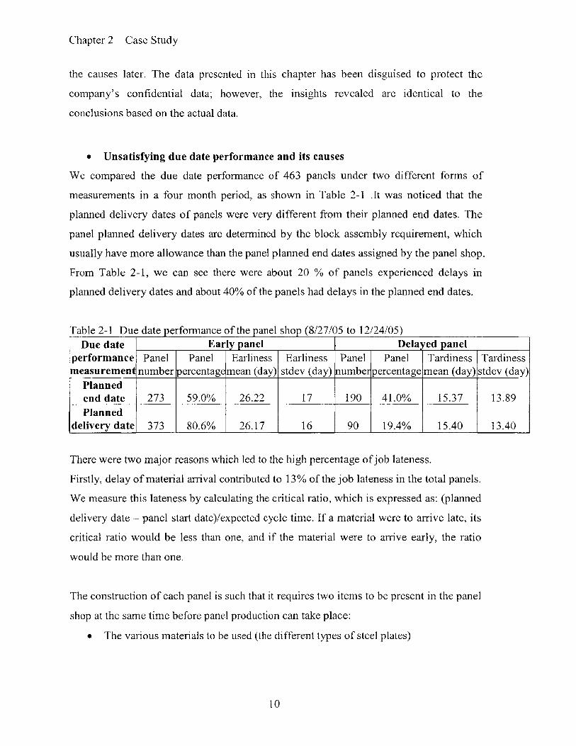
We compared the due date performance of 463 panels under two different forms of
measurements in a four month period, as shown in Table 2-1 .It was noticed that the
planned delivery dates of panels were very different from their planned end dates. The
panel planned delivery dates are determined by the block assembly requirement, which
usually have more allowance than the panel planned end dates assigned by the panel shop.
From Table 2-1, we can see there were about 20 % of panels experienced delays in
planned delivery dates and about 40% of the panels had delays in the planned end dates.
Table 2-1 Due date performance of the panel shop (8/27/05 to 12/24/05)Due date Early panel Delayed panel
performance Panel Panel Earliness Earliness Panel Panel Tardiness Tardinessmeasurement number percentage mean (day) stdev (day) number percentage mean (day) stdev (day)
Plannedend date 273 59.0% 26.22 17 190 41.0% 15.37 13.89Planned
delivery date 373 80.6% 26.17 16 90 19.4% 15.40 13.40
There were two major reasons which led to the high percentage of job lateness.
Firstly, delay of material arrival contributed to 13% of the job lateness in the total panels.
We measure this lateness by calculating the critical ratio, which is expressed as: (planned
delivery date - panel start date)/expected cycle time. If a material were to arrive late, its
critical ratio would be less than one, and if the material were to arrive early, the ratio
would be more than one.
The construction of each panel is such that it requires two items to be present in the panel
shop at the same time before panel production can take place:
* The various materials to be used (the different types of steel plates)
10
Chapter 2 Case Study
* Configuration documents (a record of the grade of steel to be used and the
dimensions of the parts to be cut).
Any delay in either item would cause the production of the panel to stall. The upstream
processes were examined and it was observed that the configuration documents were
frequently delayed. What made the situation worse was that there were constant material
shortages occurring throughout the yard. It was common to have either one of the items
arrive late, resulting in huge delays in the schedule of the panel shop.
These delays caused a shortening of the due date allowance of each panel. Since due date
performance largely depends on how much allowance is left when the material arrives,
the panel shop was frequently running behind schedule. In the 463 panels we investigated,
15% of panels had late material arrivals, while the other 12% of early panels had critical
ratios that were larger than 4. This meant that the panel shop was unable to produce the
right panels at the right time due to the mismatch of material arrivals. However, the panel
shop has little control over how the material arrives because the material delivery is
highly dependent upon lots of procedures in other departments.
Secondly, it was observed that 6% of delayed jobs with early material arrival should have
been released much earlier, but this did not occur. By only using the earliest planned end
dates to determine the release priority, the panel shop is unable to take into account the
various process time requirements of the panels. Also, the planned end dates are not the
final due dates. By such job prioritization, they are unable to guarantee that the actual
urgent panels are always to be released first.
* Unbalanced workload and its causes
Unbalanced workload in the panel shop could be indicated by the unbalanced work in
process (WIP). We compared the actual WIP and planned WIP measured by number of
panels during a four month period, shown in Figure 2-3. The actual WIP is calculated by
actual input and actual output in the panel shop. The planned WIP uses planned
input/output in the panel production schedule; it also assumes that all the panels have the
11
Chapter 2 Case Study
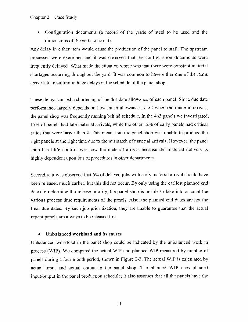
same cycle time. We can see from Figure 2-3 that planned WIP was relatively smooth
while actual WIP had very significant peaks and valleys.
6000
5000
4000
3000
2000
1000
008/27/05 09/16/05 10/06/05 10/26/05 11/15/05 12/05/05 12/25/05
Figure 2-3 Actual WIP and planned WIP measured by process time in the bottleneck station
400
0
0
350
300
250
200
150
100
50
008/27/05 09/16/05 10/06/05 10/26/05 11/15/05 12/05/05 12/25/05
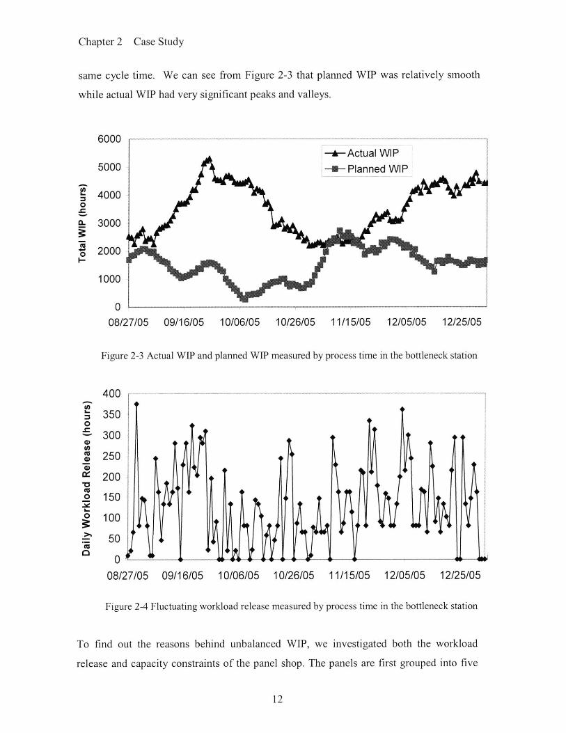
Figure 2-4 Fluctuating workload release measured by process time in the bottleneck station
To find out the reasons behind unbalanced WIP, we investigated both the workload
release and capacity constraints of the panel shop. The panels are first grouped into five
12
U)0
0
-U-Planned WIP
-a-Actual WIP
|
I
Chapter 2 Case Study
product families based on their similarities in process routes and requirements. The
grouping is validated by the descriptive statistics of cycle times for the product families
(Appendix Table 1). Based on experience, the engineers in the panel shop approved the
product family grouping and they also helped to estimate the process times of each
product family in each workstation (Appendix Table 2). The Workload of each station is
then computed by taking the average daily station process time. Capacities of the
workstations are estimated by the number of workers, work shifts and workers required
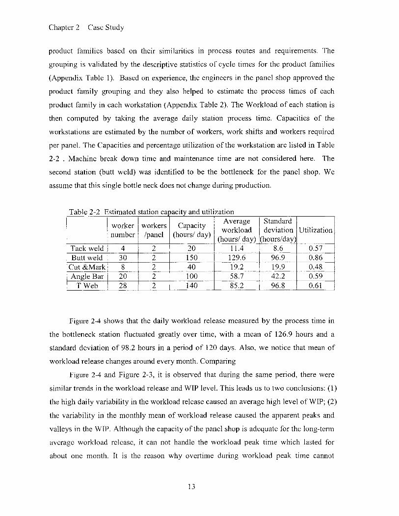
per panel. The Capacities and percentage utilization of the workstation are listed in Table
2-2 . Machine break down time and maintenance time are not considered here. The
second station (butt weld) was identified to be the bottleneck for the panel shop. We
assume that this single bottle neck does not change during production.
Table 2-2 Estimated station capacity and utilization
worker workers Capacity Average Standardwumker wpakelrshCapaty) workload deviation Utilization
number /panel (hours! day) (hours/ day) (hours/day),Tack weld 4 2 20 11.4 8.6 0.57Butt weld 30 2 150 129.6 96.9 0.86
Cut &Mark 8 2 40 19.2 19.9 0.48Angle Bar 20 2 100 58.7 42.2 0.59
T Web 28 2 140 85.2 96.8 0.61
Figure 2-4 shows that the daily workload release measured by the process time in
the bottleneck station fluctuated greatly over time, with a mean of 126.9 hours and a
standard deviation of 98.2 hours in a period of 120 days. Also, we notice that mean of
workload release changes around every month. Comparing
Figure 2-4 and Figure 2-3, it is observed that during the same period, there were
similar trends in the workload release and WIP level. This leads us to two conclusions: (1)
the high daily variability in the workload release caused an average high level of WIP; (2)
the variability in the monthly mean of workload release caused the apparent peaks and
valleys in the WIP. Although the capacity of the panel shop is adequate for the long-term
average workload release, it can not handle the workload peak time which lasted for
about one month. It is the reason why overtime during workload peak time cannot
13
Chapter 2 Case Study
completely help in processing all the jobs which adds to deteriorating due date
performance. This also causes capacity to be underutilized during low loading time. The
workload release fluctuation reveals that the workload arrival had an even higher
variability although the production schedule was planned well.
* Interplay of the two problems
The poor due date performance mutually interacted with the unbalanced workload
problem. The panel shop is under excessive pressure because 40% of panels can not meet
planned end dates and this is only made worse by the material always being late. Under
such pressure, they always attempt to push as many panels as possible into the production
line, but all this is done without effective workload control; whereas the unbalanced
workload problem worsened the due date performance.
2.4 PROPOSED SOLUTION
After identifying the due date and unbalanced workload problems and their causes, we
then propose our solution in this section and ensure that these approaches are feasible to
implement in the panel shop.
0 Objective
Our objective is to improve due date performance in the panel shop production line. The
constraints are:
o Limited capacity
o Fixed due dates
o Independent and highly fluctuating material arrival
The situation is further complicated because no advance production is possible if material
is unavailable
0 Approaches to the problem
Our approaches to the situation in the panel shop are as follows: use job prionitization and
job release control before the bottleneck.
14

Chapter 2 Case Study
The reasons and motivations to use those approaches are as below:
" Job prioritization would ensure that the most urgent jobs would be released first. We
suggest using two different criteria to determine job priority: 1) planned delivery
dates and 2) expected cycle time. They would be used to decide the flow priority of
panels. The Usage of planned delivery date also allows a longer delay window to
smooth the inputs.
" Job release control also better utilizes the capacity in the bottleneck and reduces the
chance of urgent jobs being blocked. By controlling the total workload before the
bottleneck station (butt weld) we can effectively control the output of the whole
production line.
* One particularity of the situation is that once the jobs are released into the production
line, they have to follow first-in first-out (FIFO) dispatching rule before exiting the
bottleneck station. That is because the panels will be broken if they are moved or
flipped without butt welding. Since there is a limited space between the entrance and
the bottleneck station, a sudden release of too many non-urgent jobs would result in
the new arrivals of urgent jobs having to wait longer time before being processed.
What we want to achieve is to maintain the nominal output out of the bottleneck
while keeping the workload before the bottleneck as low as possible so that the
waiting time in queue of urgent jobs is short.
2.5 SUMMARY
In the Chapter, we have discussed how job prioritization and job release control are
potential approaches to improving the due date performance in a specific job shop
environment. We emphasize that the motivations of using job release control is to
increase the prioritization flexibility and to control the cycle time of urgent jobs. This is
especially useful for the job shops where jobs enter and leave the stations on a FIFO basis.
15

Chapter 3 Analysis of Job Release Control
CHAPTER 3
ANALYSIS OF JOB RELEASE CONTROL
3.1 INTRODUCTION
This chapter will cover the analysis of the effects of job release control on the reduction
of the workload input variability. We argue that reduction of the workload variability is
the most critical factor in improving the due date performance. However, due to time
constraints faced in the project, we are unable to provide an analytical proof to support
this argument. We first begin by developing a model for a job shop in section 3.2; we
then proceed to presenting the model with a set of bounded constraints to better reflect
the situation in the panel shop in section 3.3. Section 3.4 talks about a linear control
model. A brief discussion about the key assumptions that are made in both models will be
provided in section 3.5. Finally, section 3.6 is a summary of the entire chapter.
3.2 JOB SHOP MODEL
The job shop model, as shown in Figure 3-1, consists of a job pool and a system. The
system encompasses the part of the production line in the panel shop that begins at the
entrance of the production line until the bottleneck stage. All job arrivals will first enter
the job pool to wait for release. The jobs in the job pool will be prioritized according to
their level of urgency. Right after the job pool is the release control point, which decides
how much workload should be released into the system.
J Q
A0 -o System
Control Point
Figure 3-1 Job shop model
16

Chapter 3 Analysis of Job Release Control
The assumptions we make for the job shop are:
1. The system has a single and fixed bottleneck. The stations before bottleneck are much
faster than the bottleneck so that the output of the system is predominantly decided by the
total workload before the bottleneck.
2. It is a continuous-workflow, discrete-time model. All the transition events take place at
the start of each time unit. We have set the unit of time to be in days. All the jobs are
measured by how much workload they impose on the bottleneck station. The unit of
measurement of workload is the total process time that the job requires at the bottleneck
station.
The variables for the job shop defined as follows:
A, The workload of job arrival at the beginning of day i
The workload of jobs staying in the job pool on day i
Ri The workload of released jobs on day i; the released jobs move into
the system at the beginning of day i
Qi The workload of work in process (WIP) in the system on day i
Pi The amount of production on day i
Then we have the balance equations for the job pool and the system
Ji = Ji_1 - Ri_1 + A. (3-1)
Qi = Q,_ - ±_, + R, (3-2)
Here, J1 is measured at the beginning of the day and prior to the release of the jobs. Q, is
also measured at the beginning of the day but after the release of the jobs. The quantity of
job release R. is determined by a specified job release policy. The output of the system
P; is a function of WIP Q1, and the function depends on the assumptions of production
17

Chapter 3 Analysis of Job Release Control
control and capacity limit. In the following two sections, we propose two different job
release policies which have their own assumptions on production control.
3.3 BOUNDED CONSTRAINT POLICY
We consider a situation where the job pool has an infinite buffer while the capacity and
buffer in the system are limited. We have set an upper limit for the workload of WIP in
the system. It is assumed that the system keeps producing until the output reaches the
capacity limit of the system. We can express the bounded constraints of WIP and
production as
1P= min {Q,, Co} (3-3)
Qi : wo (3-4)
where C is the capacity of bottleneck station; W is the workload limit of WIP in the
system. By converting equation (3-4) into the job release policy, we have
R, = min {J, W. - Q1 + I'} (3-5)
Equation (3-5) indicates that job release into the system depends upon the material
availability; we keep releasing the jobs into the system until the workload of the
bottleneck reaches the workload limit. One assumption that has to be made is that urgent
jobs are always released first. However, this is not shown in equation (3-5).
When W is sufficiently large, the release workload depends only on the job arrival;
When W is very small, we will have a stable queue length in the system but a low output
level. When the output rate is less than the input rate, the job in the job pool will
infinitely increase, which is unacceptable to the job shop. So the workload limit W(, has to
18
Chapter 3 Analysis of Job Release Control
be adjusted to such a value that it will maintain a nominal output level but decrease the
variability of queue length.
We were not able to get the analytic results of how the setting of workload limit will
affect the mean and variability of queue length in the job pool and the system. Instead, we
have used a spreadsheet simulation, which is based on equations (3-1) to (3-5), to see the
effects of the bounded constraint policy on the panel shop using actual historical data.
The data for job arrival and capacity limits of the job shop are listed in Table 3-1.
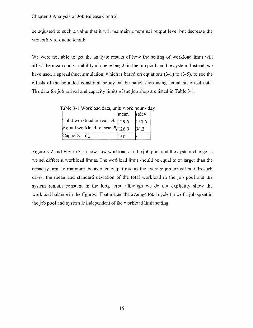
Table 3-1 Workload data, unit: work hour / daymean stdev
Total workload arrival A 129.5 150.6Actual workload release Ri 126.9 98.2
Capacity C 150 /
Figure 3-2 and Figure 3-3 show how workloads in the job pool and the system change as
we set different workload limits. The workload limit should be equal to or larger than the
capacity limit to maintain the average output rate as the average job arrival rate. In such
cases, the mean and standard deviation of the total workload in the job pool and the
system remain constant in the long term, although we do not explicitly show the
workload balance in the figures. That means the average total cycle time of a job spent in
the job pool and system is independent of the workload limit setting.
19

Chapter 3 Analysis of Job Release Control
450 400E
400 350
0 3300 >4CL)
.M 30025-25050
.E 200 0 0
.0200 0.M- 150 ...150 C..2 150.
0 10050 50 0
0 0C
0 200 400 600 800 1000 1200workload limit (hours)
Figure 3-2 Workload limit decides the average workload in job pool and in systemCo = 150 is the capacity limit. Workload limit 420 is the current practice.
Output 129.5 hours/ day
350 ----- 300
CL 300 250 E.- 4
150200 >%
150 Mo
00
0 C0 0200 400 600 800 1000 1200
workload limit (hours)
Figure 3-3 Workload limit decides the variability of workload in job pooi and
in system. C0 150 is the capacity limit. Workload limit =420 is the current
practice. Output =129.5 hours! day
Figure 3-2 and Figure 3-3 show that by decreasing the workload limit, we are able to
reduce the mean and variability of WIP in the system. Since we assume the urgent jobs
20
Chapter 3 Analysis of Job Release Control
would be always released first into the system, we can expect a shorter and more stable
shop floor time of urgent jobs with a small work load limit.
However, as the workload limits get smaller, the mean and variability of the workload in
the job pool increases. The non-urgent jobs will then experience a longer and more
fluctuated waiting time in the job pool. As we stated in Chapter one, the trade off for
improving the due date performance is to increase the waiting time of non-urgent jobs in
the job pool.
3.4 LINEAR CONTROL POLICY
In order to get an analytic result of the effects of workload control, we propose a linear
control rule and relax the capacity constraints in this section. All the definitions of
variables are the same as in last section and we add a few new variables as below
A U The workload of urgent job arrival at the beginning of day i
AN The workload of non-urgent job arrival at the beginning of day i
JU The workload of urgent jobs staying in the job pool in day i
iN, The workload of non-urgent jobs staying in the job pool in day i
So we have
A,= AU + AN, (3-6)
J,= JU, + JN, (3-7)
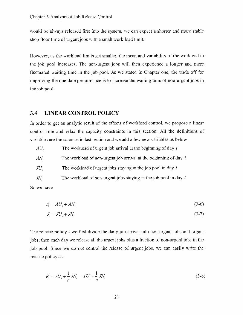
The release policy - we first divide the daily job arrival into non-urgent jobs and urgent
jobs; then each day we release all the urgent jobs plus a fraction of non-urgent jobs in the
job pool. Since we do not control the release of urgent jobs, we can easily write the
release policy as
1 1R, = JU,±- JN, = AU,-JN, (3-8)
n n
21

Chapter 3 Analysis of Job Release Control
where n is a constant not less than 1. The job release model here is similar to the
production smoothing model of Cruickshanks (1984)3. In Cruickshanks' model, n is the
length of the planning window, which is used to smooth the production level. Advanced
production is carried on during the planning window period, and the production level is
varied to match the demand rate. We apply the same smoothing principle on the job
release model. n can be treated as the length of a delay window to smooth the release of
non-urgent jobs. Advanced release is not possible, because a job can only be released
after its material arrival. With such a job release policy, urgent jobs are released first and
the release workload of non-urgent jobs is smoothed, which help to improve the due date
performance.
By substituting equations (3-6), (3-7) and (3-8) into the balance equation of job pool in
(3-1), we then obtain
JN, = JN --JN,_, + AN, (3-9)n
By iterating equation (3-9) and assuming the existence of an infinite history of job arrival,
we would write the non-urgent workload level in the job pool as
JN,-= Z 1j AN,_k (3-10)
If the non-urgent job arrivals {AN, } are independent and identically distributed (i.i.d.)
random variables with mean pN and standard deviation-N , the mean and variance of the
non-urgent workload in the job pool can be defined as:
E(JN,) = n -pN (3-1 1a)
3 Cruickshanks, A. B., R. D. Drescher and S. C. Graves. 1984. A Study of Production Smoothing in a Job
Shop Environment. Management Sci., 30, 36-42.
22

Chapter 3 Analysis of Job Release Control
2
Var(JN,) n2 N2n-1
(3-1lb)
If the urgent job arrivals {A U,} are random variables with mean pu and standard
deviation au , we can obtain the first two moments of total workload in the job pool and
job release from (3-7) and (3-8)
2
Var(J)= o-2 + n N2n -1
E(R) = pu + pN
Var(R)= o1- + 2 -N2
2n -1
(3-12a)
(3-12b)
(3-13a)
(3-13b)
For the production control, we adopt the linear control model from Graves (1986)4 in (3-
14), assuming the production is a fixed portion of the work in process remaining at the
start of the period.
(3-14)Fj = aQ,
where a is a constant, and 0 < a 1.
Combining the balance equation of the system (3-2) and equation (3-14), the production
can be expressed as
P= I>a(1-a)R_, (3-15)S =0
By substituting equations (3-10) and (3-8) into (3-15), we can link the production with
job arrival as
4 Graves, S. C. 1986. A Tactical Planning Model for a Job Shop. Oper. Res., 34, 4, pp 522-533.
23
E(J) = pu + npN

Chapter 3 Analysis of Job Release Control
P,= a(1- )o' + I a(1 -a)"A( -0 ) IANI_,_k (3-16)s=0 s=O k=O n
Since both series of {A U,} and {AN,} are i.i.d., we then find that
E(I_)= p+N (3-17)
Var(I )= a -2 2n- U (3-18)2a - (2 2n -1
Subsequently, we can get the first two moments of Q as
E(Q1)= (p+ (3-19)a
1 (2 1Var(Q,)= 2 (072 + -N2 (3-20)
2a-- a 2n-1
Although we can not compare the linear control policy with the bounded constraint
policy here because we make different assumptions on the capacity limitation of the
system, we can still gain some insights from the linear model by linking n and W
together. We can choose an appropriate value for n such that the probability of work in
process Q exceeding W is small. As the workload limit W is tightened, we have to
choose a larger n, what we get is a stable queue length in the system but an increase in
the capacity requirements and the number of jobs waiting in job pool.
The smoothing function depends on the composition of urgent and non-urgent jobs in the
job pool. One extreme case is that if all the jobs are urgent, then we have nothing to
smooth. When such a situation occurs, with capacity being limited, the due date
performance will definitely be poor. The smoothing function also depends on how we
define urgent jobs and non-urgent jobs. The prioritization function in this simple linear
24

Chapter 3 Analysis of Job Release Control
control rule does not allow us to update the job priority dynamically since we assume that
all urgent jobs are only from new job arrivals. However, in reality, some non-urgent jobs
will become urgent jobs if not treated in time. Although only the quantity of non-urgent
jobs to release is specified in equation (3-8), we should make sure that the jobs with
relatively high priority are chosen We may also adjust n and change the definition of the
urgent jobs so that the probability of the relative urgent jobs from the job pool being
selected is high.
3.5 DISCUSSION
In this section, we discuss about the relevancy of the key assumptions that we have made
in the two job release models.
Issues with the first key assumption:
The assumptions about the production control P = aQi and P, = min { Q, Co } are not
totally valid in actual operations.
Firstly, the portion ac may not be fixed when there are multiple products families and
when these product families have different planned lead times in the same station.
Depending on the job types, the maximum amount of resources it could utilize may be
different. For example, we may have 2 urgent jobs, product A and product B, that need to
be expedited. The workload of product A is twice as product B.
QA = 2QB
The maximum number of workers we can allocate to product A and product B are four
and one respectively. As a result, the production rate of product A is four times of
product B.
25
Chapter 3 Analysis of Job Release Control
P, =4PB
In this case,
QA # Q
P PB
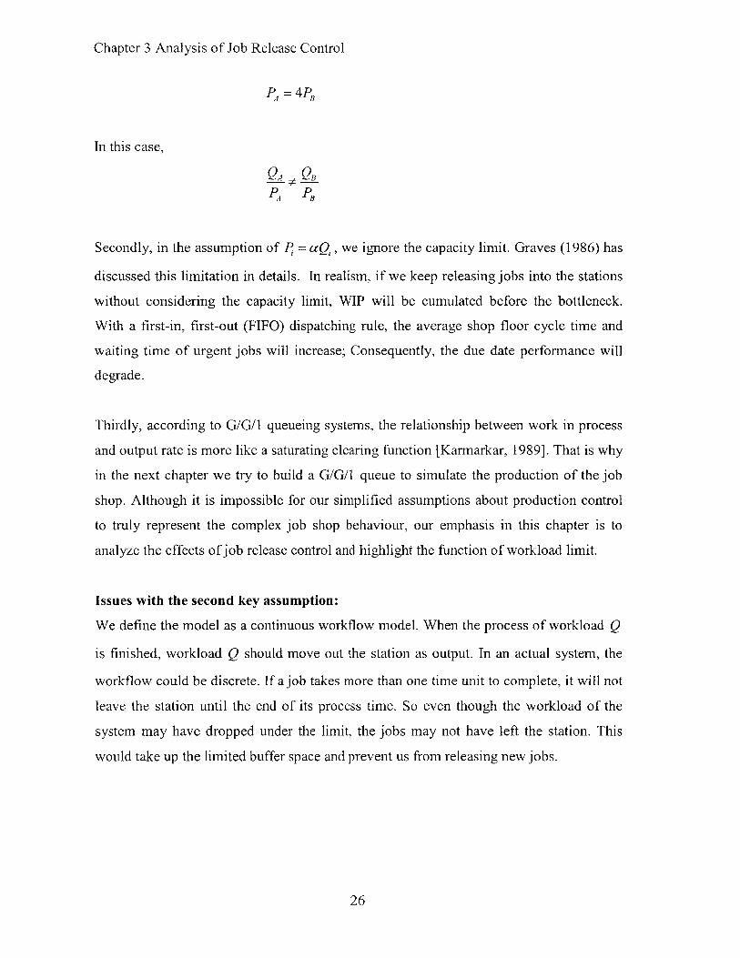
Secondly, in the assumption of Pi = aQ1, we ignore the capacity limit. Graves (1986) has
discussed this limitation in details. In realism, if we keep releasing jobs into the stations
without considering the capacity limit, WIP will be cumulated before the bottleneck.
With a first-in, first-out (FIFO) dispatching rule, the average shop floor cycle time and
waiting time of urgent jobs will increase; Consequently, the due date performance will
degrade.
Thirdly, according to G/G/1 queueing systems, the relationship between work in process
and output rate is more like a saturating clearing function [Karmarkar, 1989]. That is why
in the next chapter we try to build a G/G/1 queue to simulate the production of the job
shop. Although it is impossible for our simplified assumptions about production control
to truly represent the complex job shop behaviour, our emphasis in this chapter is to
analyze the effects of job release control and highlight the function of workload limit.
Issues with the second key assumption:
We define the model as a continuous workflow model. When the process of workload Q
is finished, workload Q should move out the station as output. In an actual system, the
workflow could be discrete. If a job takes more than one time unit to complete, it will not
leave the station until the end of its process time. So even though the workload of the
system may have dropped under the limit, the jobs may not have left the station. This
would take up the limited buffer space and prevent us from releasing new jobs.
26

Chapter 3 Analysis of Job Release Control
3.6 SUMMARY
By making an assumption on capacity and production control, we explore job release
control policies in the forms of bounded constraint and linear control. The simulated and
analytic results show that both models can effectively reduce the variability of workload
input. Although the assumptions made in the models can not completely reflect the actual
job shop behaviour, we gain a crucial understanding of the major effects of job release
control.
27
Chapter 4 Spreadsheet Simulation
CHAPTER 4
SPREADSHEET SIMULATION
4.1 INTRODUCTION
In this chapter, we build a spreadsheet simulation to see how much improvement on due
date performance is possible by applying job dispatching and workload control before the
bottleneck. Section 4.2 defines the objective of the simulation, as well as test cases and
performance measurements. Followed by that, section 4.3 describes the details about
model building and the logic inside. Model verification and validation is carried out in
section 4.4. Result analysis is represented in section 4.5. Finally, we make discussion and
conclude the chapter in section 4.6.
4.2 OBJECTIVE
The objective of the simulation is to identify the effects of job dispatching and workload
control release on the due date performance of the panel shop. We also want to
understand how the WIP, throughput and lead time change by setting different workload
limits, and ultimately, how will this affect the overall due date performance.
The performance measurements are percentage of job lateness and average negative
tardiness, which are the expected result forms of the simulation. With the historical data
of job arrival as input, we will compare the due date performance of the panel shop under
original release policy and the release policy we proposed, while maintaining the same
throughput level. The two test cases are listed in Table 4-1.
28

Chapter 4 Spreadsheet Simulation
Table 4-1 Test cases: original and proposed release policies
Job release control Workload control Job dispatching ruleOriginal Limited buffer space Earliest planned due dat(
Proposed Workload control Critical ratio
4.3 MODEL DESCRIPTION AND BUILDING
4.3.1 Model Review & AssumptionsWe simplify the actual system into a two-stage, single-server queueing model, which
includes the job pool, the tack weld station and the butt weld station. The job pool has the
capacity to hold an infinite number of panels, whereas the buffer between tack weld
station and butt weld station has limited space. The only job type is panel. The panels will
be categorized into four product families, with different means and standard deviations in
process time. Each arriving job has its own fixed due date and expected process times in
the two stations.
The workflow diagram is shown in Figure 4-1. It is a discrete-time, discrete-workflow
model. Panels are first prioritized in the job pool and then released into the tack weld
station sequentially according to the release rules. Panel enters and leaves the buffer on a
first-in, first-out (FIFO) basis. The workload control region is from the tack weld start to
the butt weld end; we can not change the sequence of the panels once they enter the tack
weld station. Subsequently, we define the controlled workload at time t as the sum of
expected butt weld process time of all the jobs in the control region.
Workload Feedback
Job Arrival Job Departure000 Job - Tack weld Buffer Butt weld - -
ReleasePrioritization Control Point Single server FIFO Single server
Figure 4-1 Workflow diagram for the first two stations in the panel shop
29

Chapter 4 Spreadsheet Simulation
Here are two clarifications for the model:
Firstly, Due to limited time in this thesis, we use single-server stations to simulate the
system. In the actual production system, the butt weld station has multiple servers. The
purpose of the thesis is to look into the relative changes of due date performances under
different release policies, so that we can recognize the importance of workload control.
Secondly, for the definition of controlled workload, we do not consider the remaining
process time of the panel in service. We claim that as long as a job stays in the
workstation, its workload remains the same as its expected process time. We expect that
the definition of controlled workload will not have much effect on the system
performance, when the bottleneck station has a fairly high utilization and the upstream
stations are fast enough. We argue that if the idleness of the bottleneck is not caused by
how we define the workload, then the approximation of workload is suitable. In our case,
the bottleneck station has a high utilization of 87% and the process time of tack weld
station is very short. If we choose an appropriate workload limit level, the bottleneck will
be kept busy most of the time with current job arrival. Also, from the real operation point
of view, it may be difficult to estimate the remaining time of manual process. Regardless
of remaining process time, we may reduce the feedback information needed and make the
workload tracking easier.
The basic assumptions we make for the model include
" The second station butt weld is the only and fixed bottleneck in the production line.
" There is independence between job arrivals and process times
" Workers with dedicated skill levels are always available during working hours
" Capacities of tack weld station and butt weld station are fixed.
" The machine break down time , repair time and set up time and the time for items
moving from one station to another station are ignored
In short, we try to build a discrete-time discrete-workflow stochastic model to simulate a
succession of panels passing through the system.
30
Chapter 4 Spreadsheet Simulation
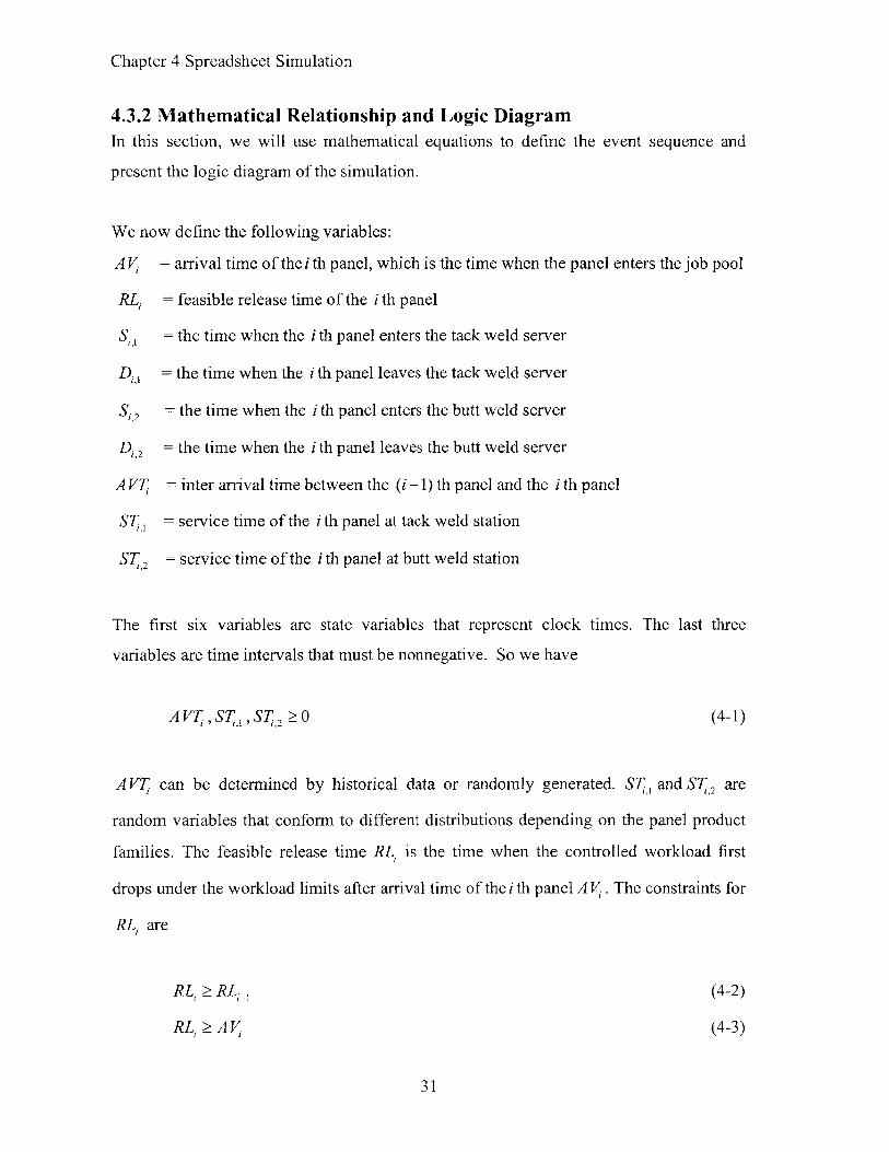
4.3.2 Mathematical Relationship and Logic DiagramIn this section, we will use mathematical equations to define the event sequence and
present the logic diagram of the simulation.
We now define the following variables:
A V = arrival time of the i th panel, which is the time when the panel enters the job pool
RL = feasible release time of the i th panel
So = the time when the i th panel enters the tack weld server
Di' = the time when the i th panel leaves the tack weld server
Si2 = the time when the i th panel enters the butt weld server
D,,2 =the time when the i th panel leaves the butt weld server
A V; inter arrival time between the (i -1) th panel and the i th panel
service time of the i th panel at tack weld station
ST,2 service time of the i th panel at butt weld station
The first six variables are state variables that represent clock times. The last three
variables are time intervals that must be nonnegative. So we have
AV7T. ,S7;l7 ,S > 0 (4-1)
A V7T can be determined by historical data or randomly generated. S7;, and ST., are
random variables that conform to different distributions depending on the panel product
families. The feasible release time RL is the time when the controlled workload first
drops under the workload limits after arrival time of the i th panel A Vi. The constraints for
RL are
RL, RL 1 (4-2)
RL1 > A V (4-3)
31

Chapter 4 Spreadsheet Simulation
Assuming the panels have been prioritized in the job pool, we have five independent
equations to represent the mathematical model. The sequential panel arrival to the job
pool can be described as
AV, = AV_, + AVT (4-4)
The arrivals and departures of tack weld station can be expressed as
Si' = max(RLi , Di-,_) (4-5)
D = SI + S (4-6)
(4-5) means that the service start time of panel i can not be earlier than the service end
time of panel (i -1) in tack weld station, nor the feasible release time. Similarly, we have
the arrivals and departures of butt weld station as
Si,= max(D 1 , D, 1 2 ) (4-7)
Du" = Si, + ST-, (4-8)
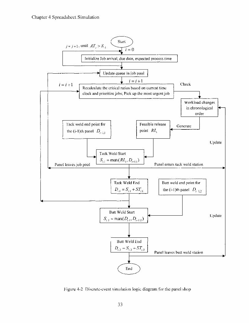
The logic diagram of the simulation is presented in Figure 4-2. At the times of transitions,
the simulation clock is fast forwarded to the time when the next event is scheduled to
happen. It should be noted that the clock of arrival of new jobs is not synchronous with
the clock of new job release. We should generate job arrivals until the latest time of job
arrival is later or equals to the current feasible release time. However, since we use
historical job arrival data in the simulation, we do not have to worry about that problem.
32
Chapter 4 Spreadsheet Simulation
j=j+j, until A T > S yStart
Initialize Job arrival, due date, expected process time
Update queue in job pool
i=i +1Recalculate the critical ratios ba
clock and prioritize jobs; Pick u
Tack weld end point for
the (i-l)th panel D,11
Panel leaves job pool
Tack Weld Start
Si = maX(RL,,Di_
4,Tack Weld End
D, = S +ST.
Butt Weld Start
S.2 =max(D_,1 D,.)
sed on current time
pthe most urgent job
Workload changes
in chronological -order
Feasible release Generate
point RL,
Update
Panel enters tack weld station
Butt weld end point for
the (i-l)th panel D,- 2
Update
4FButt Weld End
D2 = Si + ST 2Panel leaves butt weld station
End
Figure 4-2 Discrete-event simulation logic diagram for the panel shop
Check

Chapter 4 Spreadsheet Simulation
4.3.3 Spreadsheet ImplementationWe build the simulation in Microsoft Excel. The simulation has three modules: the job
pool, the workload look-up table and the workstations. Visual Basic Application (VBA)
programming in Excel is used to set the time sequence of events to follow the logic
diagram. The snapshot of the spreadsheet simulation is shown in Figure 4-3. We now
explain the functions of the three modules:
The job pool dynamically updates all the jobs that are available for release. New arrived
jobs at the beginning of the day are added with the remaining jobs in the job pools. The
program will then recalculate the critical ratios of all the jobs based on their due dates,
expected cycle time and current time clock. The expected cycle time for each product
family is fixed and well estimated from the results of adequate trials of simulations. The
job with the highest priority is selected to wait for release. After a job is released into tack
weld station, we delete that job from the job pool.
The workload look-up table records the changes in controlled workload in chronological
order. Based on the definition of workload we made in last section, the state of controlled
workload changes only when a job enters tack weld station and leaves butt weld station.
Thereby, we arrange the tack weld start-time and butt weld end-time in chronological
order; meanwhile we record the workload input for each tack weld start point and the
workload output for each butt weld end point. Then the controlled workload at a specific
time t equals to the cumulative workload inputs minus cumulative workload outputs not
later than time t, which can be easily calculated in excel.
The workstations include release decision point and processes in tack weld station and
butt weld station. Each row in the spreadsheet corresponds to a panel and records all the
panel attributes and event times. For the job with arrival time A Vi and expected workload
J'Jj that is ready to release, we check the workload look-up table and generate the feasible
release time RLi which satisfies all the following conditions: (1) it is the earliest time
which is greater than the arrival time A Vi; (2) it is equal to or greater than last feasible
34
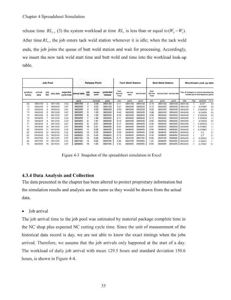
Chapter 4 Spreadsheet Simulation
release time RLi_ (3) the system workload at time RL is less than or equal to (W - W).
After time RL, the job enters tack weld station whenever it is idle; when the tack weld
ends, the job joins the queue of butt weld station and wait for processing. Accordingly,
we insert the new tack weld start time and butt weld end time into the workload look-up
table.
Tack Weld Station Butt Weld Station Woorkload Look up tabli
product arrival job expected job release potiential Tack service . Butt time of changes in control workload (be
family date NO due date cycle time arrival date NO point release Service start service end Service service start service end release point and departure point
Point wOrkload point tack point point butt point point tie Flag wokload CM w0.110.310.530.420.350.110.150.170.010.010.090.130.170.460.42
08/01/0508/02/0508/03/0508/03/0508/03/0508/04/0508/04/0508/04/0508/04/0508/06/0508/06/0508/06/0508/07/0508/07/0508/08/05
08/01/0508/02/0508/03/0508/03/0508/04/0508/04/0508/04/0508/04/0508/04/0508/06/0508/06/0508/06/0508/07/0508/08/0508/08/05
0.100.120.020.980.090.130.500.340.470.040.080.160.091.240.03
08/01/0508/02/0508/03/0508/03/0508/04/0508/05/0508/05/0508/05/0508/05/0508/06/0508/06/0508/06/0508/07/0508/08/0508/09/05
08/01/0508/02/0508/03/0508/04/0508/05/0508/05/0508/05/0508/05/0508/06/0508/06/0508/06/0508/06/0508/08/0508/09/0508/09/05
08/01/0508/01/0508/02/0508/02/0508/03/0508/03/0508/03/0508/03/0508/04/0508/04/0508/04/0508/04/0508/04/0508/05/0508/05/05
-1
-1
-1
-1
-1
-1
0.077-0.076670.526533-0.526530.5265330.526533-0.526530.5265330.3798670.379867
0.20.2
-0.52653-0.52653-0.37987
0.10.10!010!11011.1
1.'1.1
2.(2.11.0:
Figure 4-3 Snapshot of the spreadsheet simulation in Excel
4.3.4 Data Analysis and CollectionThe data presented in the chapter has been altered to protect proprietary information but
the simulation results and analysis are the same as they would be drawn from the actual
data.
0 Job arrival
The job arrival time to the job pool was estimated by material package complete time in
the NC shop plus expected NC cutting cycle time. Since the unit of measurement of the
historical data record is day, we are not able to know the exact timings when the jobs
arrived. Therefore, we assume that the job arrivals only happened at the start of a day.
The workload of daily job arrival with mean 129.5 hours and standard deviation 150.6
hours, is shown in Figure 4-4.
35
Job Pool Release Point
A2T3T3T3T3T2T2T1T1A2A2A2T3A2T3
08/01/0508/02/0508/03/0508/03/0508/03/0508/04/0508/04/0508/04/0508/04/0508/06/0508/06/0508/06/0508/07/0508/07/0508/08/05
23456789
10111213141516
08/11/0508/04/0508/05/0508/12/0508/12/0508/12/0508/12/0508/13/0508/13/0508/10/0508/20/0508/20/0508/14/0508/12/0508/15/05
3.023.673.673.673.673.333.333.073.073.023.023.023.673.023.67
08/01/0508/02/0506/03/0508/03/0508/03/0508/04/0508/041050810410508/0410508/06/0508/08/0508/06/0508/07/0508/07/0508/08/05
23456789
10111213151416
0.080.530.531.051.051.431.812.012.210.280.350.430.080.601.05
08/01/0508/01/0508/02/0508/03/0508/03/0508/03/0508/04/0508/04/0508/04/0508/04/0508/06/0508/06/0508/06/0508/07/0508/07/05

Chapter 4 Spreadsheet Simulation
800 ---
700
o 600
- 500
400
3000x 2000
100
008/27/05 09/16/05 10/06/05 10/26/05 11/15/05 12/05/05 12/25/05
Figure 4-4 Daily workload arrival at the job pool measured by process time in bottleneck station
0 Job release
We will use the record of actual job release in the original release policy test case. The
daily workload release is shown in Figure 2-4 in the Chapter 2. In the test case of
workload control, the job release time will be decided by the workload status in the
system.
0 Process time
The means of process time for each product family in tack weld station and butt weld
station were estimated by the engineers in the panel shop, as listed in Table 4-2. We
estimated the coefficients of variance of the process times. Since we use single server for
butt weld station, the process times in butt weld station will be adjusted into 1/ n of the
original process times, where n is the original server number. In the simulation, the
process times of the panels will be random numbers that conform to normal distribution.
We will do sensitivity analysis about the process times in the model validation.
Table 4-2 Estimated process time statistics (unit: day)
Product mean coefficientfamily A2 TI T2 T3 of variance
Tack weld 0.2 0.15 0.2 0.4 0.74
Butt weld 0.575 1.5 2.849 3.949 0.76
36
Chapter 4 Spreadsheet Simulation
9 Due date
Because we only model the first two stations, we are unable to compare the due date
performance in the simulation and in the actual system. Instead, we will set a new due
date for each job using its original critical ratio, expected cycle time and actual release
time.
In short for the data input, the job arrival, due dates and station capacities are fixed. The
only stochastic factor is the process time of each job, which conforms to normal
distribution. We then apply different job release rules to see the due date performance.
4.4 MODEL VERIFICATION AND VALIDATION
4.4.1 Model VerificationWe verify the model by checking for reasonable outputs in three separate tests.
Test 1: Job priority update
We have arranged one hundred non-urgent jobs in day 1 and one urgent job in day 2.
After processing the first three relatively urgent jobs in day 1 and the time clock moves to
day 2, the program will then pick up the urgent job of day 2, and then continued to
process the rest of the remaining jobs. This proves that the function of job sequencing
works well.
Test 2: Process
We now use constant release and constant process time as inputs. As expected, the
waiting time before the tack weld station and the butt weld station is zero; the station
utilization is exactly equal to arrival rate over service rate.
Test 3: Workload control
We then set different workload limits. In all cases, the workload in the stations is kept
well below the workload limits.
37

Chapter 4 Spreadsheet Simulation
4.4.2 Model Validation
We validate the model from three aspects: extreme condition tests, comparison with other
models and sensitivity analysis.
0 Extreme condition tests
In the first test we will set the arrival rate to be larger than the service rate; then in the
second test, we will set the workload limit to be less than the arrival rate. In both cases,
we expect to see that the accumulated jobs in the job pool go to infinity, which is
indicated by the increasing job waiting times in the job pool, as shown in Figure 4-5.
40
"0 35 +*AWL<AR
o 30 -*-SR<AR0 250
250
S20
15
40
~10
08/27/05 09/16/05 10/06/05 10/26/05 11/15/05 12/05/05 12/25/05
Figure 4-5 Increasing job waiting time in the job pool in two extreme condition testsTest 1 WL<AR: workload control is less than job arrival rate; utilization of tackweld station = 0.46; utilization of butt weld station = 0.6. Test 2 SR<AR: servicerate in the bottleneck is less than job arrival rate; utilization of tack weld station= 0.46; utilization of butt weld station = 1. The job process times in test I are thesame as in test 2.
A comparison with other models
We examine how the shop floor cycle time and waiting time in the job pool change as we
set different workload limits before the bottleneck station. We then compare the queueing
simulation results with the outputs from the bounded constraint model in Chapter 3. The
bounded constraint model is a continuous-workflow, single-stage and bounded capacity
model, while the queueing simulation here is a discrete-workflow, two-stage and
38

Chapter 4 Spreadsheet Simulation
saturating capacity model. We find that the trends in the cycle times versus the workload
limits in the queueing model (see Figure 4-6 and Figure 4-7) are still quite similar to that
of controlled workloads changes versus workload limits in the bounded constraint
model( see Figure 3-2 and Figure 3-3). As the workload limit in the bottleneck station
increases, the mean and standard deviation of shop floor cycle times increase, while the
mean and standard deviation of waiting times in the job pool decrease. Since we have
assumed that the capacities for both stations are fixed, cycle time is proportional to
workload in the long term. In all the tests, we used the same set of process times.
4 -. .3 *
3
4
R~ *.~* I
NI N
WL=2.8d: WL= 11 d
0 4 8
Workload L imit (day)
Figure 4-6 Workload limit decides the average waiting time in job pool and averageshop floor cycle time. 'WL' stands for workload limit. When the workload limit islarger than 2.8 days, the sums of average waiting time in job pool and shop floor cycletime remain constant. When the workload limit is less than 2.8 days, the total cycletime starts to increases. Workload limit = 11 days is the current practice.
39
0
C
0C _
0
01
0
3.
2 5
2s
06
A~
-36E
-3 0
-25
-2
-1 15
0-
012
i
10
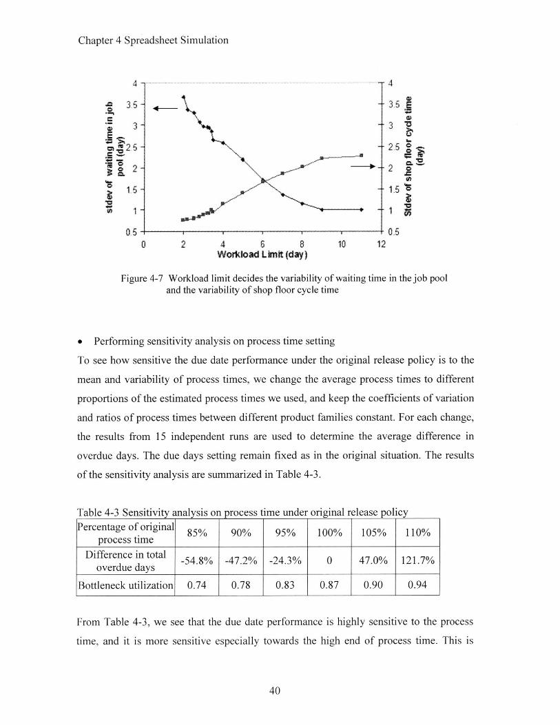
Chapter 4 Spreadsheet Simulation
4-4
A - 3
0 205
0 2 4 6 8 10 12Workoad L imit (day)
Figure 4-7 Workload limit decides the variability of waiting time in the job pooland the variability of shop floor cycle time
SPerforming sensitivity analysis on process time setting
To see how sensitive the due date performance under the original release policy is to the
mean and variability of process times, we change the average process times to different
proportions of the estimated process times we used, and keep the coefficients of variation
and ratios of process times between different product families constant. For each change,
the results from 15 independent runs are used to determine the average difference in
overdue days. The due days setting remain fixed as in the original situation. The results
of the sensitivity analysis are summarized in Table 4-3.
Table 4-3 Sensitivity analysis on process time under original release policyPercentage of original 85% 90% 95% 100% 105% 110%
process timeDifference in total -54.8% -47.2% -24.3% 0 47.0% 121.7%
overdue days
Bottleneck utilization 0.74 0.78 0.83 0.87 0.90 0.94
From Table 4-3, we see that the due date performance is highly sensitive to the process
time, and it is more sensitive especially towards the high end of process time. This is
40

Chapter 4 Spreadsheet Simulation
reasonable because as the process times increase, the bottleneck utilization will approach
to one, causing the job cycle times to increase dramatically. Therefore, we need to choose
the process times carefully. Although the only data available to us is the estimated
process time, by setting the new due dates according to the expected cycle time and
critical ratios of the jobs, we are able to maintain the urgencies of the jobs to be the same
as the ones in the original system.
4.5 SIMULATION OUTPUT ANALYSIS
* Warming-up period and run length
Warm-up period: 20 days
Total simulation time: 120 days
Replicate numbers: 24
0 The comparison of due date performances under different release policies
The three job release policies that were simulated here are
a) Original release: historical release data
b) CR: historical arrival data and critical ratio dispatching rule.
c) CR+WLC: historical arrival data, critical ratio dispatching rule and workload
control release.
In each independent run, we first generate the process times randomly for each job
according to its product family. We then apply different release policies to the same set of
job process times. The total overdue days under the three release policies in 24 runs are
shown in Figure 4-8. The average output levels are maintained constant throughout all
the runs. The workload limit is set as 2.8 days.
41
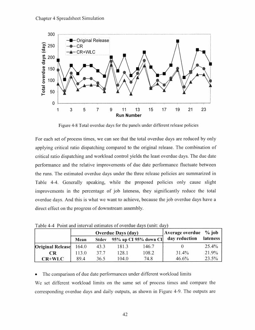
Chapter 4 Spreadsheet Simulation
300-- Original Release
>250 -4- CR-*- CR+WLC
200
150
> 1000
0 50
01 3 5 7 9 11 13 15 17 19 21 23
Run Number
Figure 4-8 Total overdue days for the panels under different release policies
For each set of process times, we can see that the total overdue days are reduced by only
applying critical ratio dispatching compared to the original release. The combination of
critical ratio dispatching and workload control yields the least overdue days. The due date
performance and the relative improvements of due date performance fluctuate between
the runs. The estimated overdue days under the three release policies are summarized in
Table 4-4. Generally speaking, while the proposed policies only cause slight
improvements in the percentage of job lateness, they significantly reduce the total
overdue days. And this is what we want to achieve, because the job overdue days have a
direct effect on the progress of downstream assembly.
Table 4-4 Point and interval estimates of overdue days (unit: day)
Overdue Days (day) Average overdue % jobMean Stdev 95% up CI 95% down CI day reduction lateness
Original Release 164.0 43.3 181.3 146.7 0 25.4%CR 113.0 37.7 128.1 108.2 31.4% 21.9%
CR+WLC 89.4 36.5 104.0 74.8 46.6% 23.5%
0 The comparison of due date performances under different workload limits
We set different workload limits on the same set of process times and compare the
corresponding overdue days and daily outputs, as shown in Figure 4-9. The outputs are
42

Chapter 4 Spreadsheet Simulation
measured by the expected process time in butt weld station of the job output. When the
workload limit is decreasing and the average output remains constant, the total overdue
days are reduced. However, if the workload limit is too small, such that the output level
begins to decrease, the total overdue days will increase. The reason is that: without
deterioration in the output level, a small workload limit increases the probability that the
newly arrived urgent jobs will be selected and processed soon; on the other hand, with
too small a workload limit, jobs will be hindered from being released and the resources
can not be utilized well.
150 - - - -.- - - - - -- - 0.825
140 0.820
130 0.815 '(U
S120 0.810
1 110 0.805 o
0 100 0.800-i- Overdue days
1-90 -U- Daily output 0.795
80 0.7900 2 4 6 8 10 12
Workload Limit (day)
Figure 4-9 Overdue days and daily outputs under critical ratio dispatching rule anddifferent workload limits, based on the same set of job process times.
It is difficult to determine the optimal workload limits, especially in a job shop with high
variability in job arrival and process. We need to detect the switch of long-term job
arrival rate to adjust the workload limit, such that the average job output rate equals to
average arrival rate. In addition, the variability of process time will decide the level of the
workload limit so that the average output rate is maintained. With a non stationary job
arrival and job process, the workload limits have to be changed dynamically.
43

Chapter 4 Spreadsheet Simulation
4.6 CONCLUSION
We have built a spreadsheet queueing simulation to determine whether the combination
of workload control and critical ratio dispatching is able to improve due date performance
greatly and whether it is better than applying critical ratio dispatching alone. We have
found that it is. The setting of workload limits affects the decision of job sequencing and
the due date performance. In order to achieve the best due date performance, we should
choose the smallest workload limit that maintains the nominal output levels. This
conclusion is based on the assumption of fixed capacity, steady job arrival and process.
44

Chapter 5 Summary and Suggestions
CHAPTER 5
SUMMARY AND SUGGESTIONS
5.1 SUMMARY FOR THE THESIS
In the last chapter, we summarize the thesis and make suggestions to the company. Also,
we propose several possible ideas for the future research.
In the thesis, we have primarily studied the effects of job release control in a make-to-
order job shop with fixed due dates and limited capacity. A lot of research about job
release control considers that the jobs are always available to be released to maintain a
large job pool or constant work in process in the system. However, we focused on the job
shop which has little control about the timing and quantity of fluctuating job arrival. We
employed a bounded constraint model and a linear control model with different
assumptions about production control in a single stage system. From our simulated and
analytic results, we found that the combination of job dispatching and workload control
can effectively control the variability of shop floor workload and production. We also
showed the trade-off between workload limit setting and the queueing length of the jobs
waiting to be released. We then built a spreadsheet simulation of a two-stage, single-
server queueing model to show the benefits of job release control for due date
performance improvement.
Clearly, how to set workload limits and workload norm depends on the job shop
environment. Also, the effects of job release control are greatly affected by the status of
job arrival and the tightness of due date setting. To implement the job release control, we
require that not all the job arrivals are urgent so that we can delay the release of some
non-urgent jobs. It is complicated to decide what faction of jobs can be urgent so that the
workload control will be effective to improve the due date performance. Assuming the
jobs are always prioritized before they entered the first station, we provide some intuitive
45
Chapter 5 Summary and Suggestions
analysis. Firstly, we are clear that workload control will not help to reduce tardiness in
two extreme cases: 1) all the jobs are not urgent and 2) all the jobs are urgent and with
the same urgency. Here, the urgency is relative. Even all the jobs are urgent, applying
workload control will still improve the due date performance if the jobs have different
urgencies. Secondly, the faction of urgent jobs that the work shop can handle depends on
the balance of workload arrival and urgent job arrival. In other words, it is not good that
the peaks of workload arrival lasts for a long time, or the urgent jobs keep arriving
intensively. It would be worse when there are overlaps between the peaks of workload
arrival and urgent job arrival. When the capacity is not sufficient for the workload peak
time, less urgent jobs help to alleviate the pressure on due date performance.
We could either urge the job arrival to be earlier or increase the planned delivery time to
reduce the portion of urgent jobs. The other method is to expand capacity or increase
capacity flexibility so as to shorten the shop floor cycle time. Both approaches aim to
increase the critical ratio of a job.
5.2 SUGGESTIONS FOR THE COMPANY
Based on the study during the internship project, we made several suggestions concerned
about the production planning and scheduling for the company, and we hope these
suggestion would be helpful to improve the performance of the company.
Outside the panel shop:
" Smooth the MPS by coordinating different projects and sub projects.
" Make sure that the material packages arrive on time and follow the schedule.
Reduce the material arrival variability.
" Predict the peak demand period and make capacity expansion decision earlier.
Inside the panel shop
* Group panels into product families and consider the cycle time difference into the
panel fabrication schedule.
46

Chapter 5 Summary and Suggestions
* Estimate the nominal capacity and the maximal capacity expansion limits as
accurate as possible. Use process time rather than panel number to estimate the
capacity.
* Use the planned delivery dates and expected product family cycle time to set the
flow priority of panels.
* Apply workload control before the bottleneck station. Firstly, we need to define
the form of workload. The workload of panels could be roughly estimated by the
size of the panels. For example, if all the panels can be grouped as big panels,
middle panels and small panels, we could use a small panel as the workload unit
to measure the workload of big and middle panels. Then the workload limit can
be several combinations of the panel mix. Secondly, we may first set the
workload limit high enough and then gradually reduce it to find out the
appropriate value while maintaining the average output rate.
5.3 FUTURE RESEARCH
There are several possible extensions that may improve and enrich the job release control
model we applied in the thesis.
(1) Floating or multiple bottlenecks
In the thesis, we only consider the production line which has a single and fixed
bottleneck so we have a single constraint on workload and a fixed control region. In
actual systems, there may be multiple bottlenecks; therefore, we might have multiple
constraints and we may need to pick up the bottleneck we want to emphasize. Also, the
bottleneck may not be fixed due to the change of product mix. We may then need to solve
the problem of detecting the bottleneck quickly and accurately.
(2) Non stationary job arrival
In the thesis, we assume the job arrival is stationary; and the setting of workload limit is
decided by the mean and standard deviation of job arrival. If the job arrival is not
stationary, we may also need to adjust the workload limit dynamically and continuously.
Similarly, we may also consider the situation when the arrival of urgent jobs is not
stationary.
47

Chapter 5 Summary and Suggestions
(3) Decision making affected by tightness of due dates
We have not studied how the tightness of due dates will affects the decision in job release
control. When most of the jobs are urgent, it may not suitable to control the workload by
delaying some of the incoming jobs. We may need to figure out other production control
methods when the tightness of due dates changes.
48

Appendix
APPENDIX
NC Tack Butt Cut & Angle Bar T Web Pick upCutting Weld Weld Mark outfitting outfitting QA&QC
Steel plates B1
Figure 1 workstations and buffer configuration in the panel shop. Rectangle denotesworkstation, while circle denotes buffer. Bottleneck is the butt weld station with highestutilization and limited station size.
Table 1 description statistics of product family cycle time for the panels in the panel line
Big Sub Plate Area Cycle Time (day)groups group (m^2) Number Mean Stdev C.O.V Min median Max
No Al PA<5 87 8.03 1.78 0.22 5 9 12T-web A2 PA>5 131 12.42 3.42 0.27 6 12 20
T1 PA<17 107 19.56 6.45 0.33 9 19 32T-web T2 17<PA<54 152 23.73 7.43 0.31 11 23 38
T3 PA>54 132 27.71 6.67 0.24 23 27 41
49
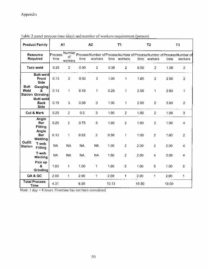
Appendix
Table 2 panel process time (day) and number of workers requirement (person)
Product Family Al A2 TI T2 T3
Resource Process Number Process Number of Process Number of Process Number of Process Number ofRequired time o time workers time workers time workers time workers
______________workers
Tack weld 0.25 2 0.50 2 0.38 2 0.50 2 1.00 2
Butt weldFront 0.13 2 0.50 3 1.00 1 1.00 2 2.00 2Side
Butt GaugingWeld & 0.13 1 0.19 1 0.25 1 2.00 1 2.00 1
Station GrindingButt weld
Back 0.19 3 0.50 3 1.00 1 2.00 2 3.00 2Side
Cut & Mark 0.25 2 0.5 3 1.00 2 1.00 2 1.00 3
AngleBar 0.25 2 0.75 5 1.00 2 1.00 2 1.00 4
FittingAngle
Bar 0.13 1 0.63 2 0.50 1 1.00 2 1.00 2Welding
Outfit T-webStation Fitting NA NA NA NA 1.00 2 2.00 2 2.00 4
TWei NA NA NA NA 1.00 2 2.00 4 3.00 4
Pick up& 1.00 1 1.00 1 1.00 3 1.00 5 1.00 5
Grinding
QA & QC 2.00 1 2.00 1 2.00 1 2.00 1 2.00 1
Total Process 4.31 6.56 10.13 15.50 19.00TimeNote: 1 day =8 hours. Overtime has not been considered.
50

References
REFERNCES
Andrew, F. S., 2001, Spreadsheet Simulation, Proceedings of the 2001 Winter Simulation
Conference, 74-79
Bechte, W., 1988. Theory and Practice of Load-oriented Manufacturing Control.
International Journal of Production Research 26: 375-395
Bertrand, J.W.M. and Wortmann, J.C., 1981. Production Control and
Information Systems for Component-manufacturing Shops. Dissertation. Elsevier,
Amsterdam, The Netherlands.
Blackstone, J.H., D.T. Philips, and G.L.Hogg. 1982. A state-of-the-art Survey of
Dispatching Rules for Manufacturing Job Shop Operations. International Journal of
Production Research 20(1): 27-45
Brian, G.K., 2000, Modeling Input-output Workload Control for Dynamic Capacity
Planning in Production Planning Systems. International Journal of Production
Economics 68(2000)73-93
Cruickshanks, A. B., R. D. Drescher and S. C. Graves. 1984. A Study of Production
Smoothing in a Job Shop Environment. Management Sci., 30, 36-42.
Graves, S. C. 1986. A Tactical Planning Model for a Job Shop. Oper. Res., 34, 4, pp 522-
533.
Hopp, W. J., M. L. Spearman. 2000. Factory Physics: Foundations of Manufacturing
Management, 2 "d edn, McGraw-Hill.
Karmarkar, U.S. 1993. "Manufacturing Lead Times, Order Release, and Capacity
Loading. " Logistics of Production and Inventory, S. Graves, A. H. G. Rinnooy Kan and
51

References
P. Zipkin (eds.), Handbook in Operations Research and Management Science, Vol. 4,
North Holland.
Karni, R. 1982. Capacity requirements planning - A systematization. International
Journal ofProduction Research 20(6): 715-739
Martin, L., 2005, Parameters and Sensitivity in Workload control. International Journal
of Production Economics In Press, Corrected Proof
Tatsiopoulos, I.P., 1993. Simplified Production Management Software for the Small
manufacturing firm. Production Planning Control 4(1): 17-26
Thomas A. Grossman, Jr., 1999, Teachers' Forum: Spreadsheet Modeling and Simulation
Improves Understanding of Queues. Interfaces archive Volume 29, Issue 3 88-103
Wein, Lawrence M. 1988. Scheduling Semiconductor Wafer Fabrication, IEEE
Transactions of Semiconductor Manufacturing 1, 115-130.
Wight, 0. 1970. Input/Output control: A Real Handle on Lead Time. Production and
Inventory Management Journal 11(3): 9-31
52