productivity and real exchange rate movements for the

Productivity and Real Exchange Rate Movements for the ASEAN and SAARC

Countries: Revisiting the Balassa-Samuelson Hypothesis

I. Introduction

Exchange rate equilibrium is a longstanding notion which has always been imperative in

explaining the mechanism of economic and financial stability of a region. The long run dynamics

of exchange rate can be traced back to 1922 when Gustav Cassel first introduced the concept of

Purchasing Power Parity (PPP) which is regarded to be the best manifestation of potentially

equilibrium exchange rates. This theory states in a macroeconomic environment where exchange

rates and commodity prices are perfectly flexible and cross-country trade is absolutely

frictionless, the relative prices between countries are tend to be stable or stationary over time.

This theory can be seen as a long term tendency of the equilibrium exchange rate.

Cross country price levels in connection with bilateral exchange rate movements do not

only represent PPP-phenomenon but also undertake the discussion of relative sectoral prices

(tradables and non-tradables). Balassa (1964) and Samuelson (1964) were the first ones who, in

the context of exchange rate and relative sectoral price differentials, attributed these price

differentials to differentials in economic development which are likely to persist for longer

periods. One country being more productive than the other, the former’s non-traded sector is

most likely to face a sharper rise in price levels in comparison to the later one, resulting in a real

appreciation of former country’s exchange rate. In simpler words, Balassa and Samuelson (1964)

provided the first realistic explanation of why the theory of absolute PPP is flawed in the

perspective of equilibrium exchange rates.

1

As discussed earlier, the absolute version of PPP can be realized only by assuming spatial

arbitrage in a well-connected and perfectly competitive, frictionless world economy, so that the

relative prices of a common basket of goods across countries are equalized when quoted in a

common currency. As an explanation to this, consider a situation where the price of nth good at

home is given as 𝑝𝑝𝑛𝑛 and in foreign the same good has a price 𝑝𝑝𝑛𝑛′ . E is the bilateral exchange rate

between home and foreign defined as units of home currency per unit of foreign currency. P and

P* are the aggregate price level indices for all the goods produced locally at home and abroad

quoted in their local currencies. With the given specifications, absolute PPP can be validated if

the two prices (in terms of domestic currency) for each good get equalize across countries,

provided every type of market frictions and rigidities are absent. The common basket of goods

across two countries, if comprising of exactly identical goods with commonly used weights, then

the law of one price i.e. price equalization (between 𝑝𝑝𝑛𝑛 and 𝑝𝑝𝑛𝑛′ ) for nth good can be taken in a

broader perspective of equalization of aggregate price indices (P and P*) giving rise to well

known absolute PPP formulation of 𝐸𝐸 = 𝑃𝑃𝑃𝑃∗

. Thus, absolute version of PPP states that assuming

no market frictions and rigidities, the relative price of a common basket of goods across

countries measured in a common currency will always be equal i.e. 𝑃𝑃𝐸𝐸𝑃𝑃∗

= 1

In their classical articles The Purchasing Power Parity Doctrine: A Reappraisal by Bela

Balassa and Theoretical Notes on Trade Problems by Paul A. Samuelson, published in 1964,

first time provided the most obvious reasoning in the form of productivity-exchange rate pass-

through that why absolute version of PPP is unlike to hold in long run. The introduced the factor

of cross country sectoral productivity growth differential between traded and non-traded sectors

as an important factor responsible for bringing systematic biases into the relationship between

cross country relative prices of tradables and exchange rate. They regarded this sectoral

2

productivity growth bias, vital for bringing undesirable alternations in an economy’s internal

price mechanisms.

According to their model, an economically advanced country i.e. high income country is

likely to be technologically more sound and advanced as compared to a low income economy.

However, this technological advancement will not be uniform across all the sectors of economy.

It is likely to be more pronounced for tradable sector of the economy in comparison to non-

tradable one. Assuming purchasing power parity with no market friction or rigidities, the prices

of tradables from various countries will be equalized as they are traded in international market.

However, this will not be the situation for non-tradables for which law of one price does not

hold. Thus if the home country is growing more in terms of traded sector productivity relative to

its trading partner, it will cause the domestic wage rate of traded sector to increase. This wage

rise will bring supply-side inflation for non-traded sector only pulling their prices upwards

(prices of traded sector being determined internationally will not take up this influence), thus

causing the domestic real exchange rate to appreciate relative to its trading partners. Hence long

run cross country sectoral productivity differentials will make long run exchange rate to see trend

deviations from PPP.

∆𝑅𝑅𝐸𝐸𝑅𝑅𝑡𝑡 = ∆𝑒𝑒𝑡𝑡 + 𝛿𝛿�

𝛶𝛶�(1 − 𝛽𝛽)��∆�̃�𝐴𝑡𝑡𝑇𝑇∗ − ∆�̃�𝐴𝑡𝑡𝑁𝑁∗� − �∆�̃�𝐴𝑡𝑡𝑇𝑇 − ∆�̃�𝐴𝑡𝑡𝑁𝑁�� ----------------------- (1)

where

𝑟𝑟𝑒𝑒𝑟𝑟𝑡𝑡= Bilateral real exchange rate

𝐴𝐴𝑡𝑡𝑠𝑠�= Average labor productivity, s = traded and non-traded sectors

1 − 𝛽𝛽 = Share of non-tradables in consumption basket

* = trading partner (reference country)

3

The above equation represents that if 𝑎𝑎𝑇𝑇 is found to be growing at a faster pace than 𝑎𝑎𝑇𝑇∗

the domestic wage rate will rise in comparison to the international one. If it is also a situation

that 𝑎𝑎𝑇𝑇 is growing faster than 𝑎𝑎𝑁𝑁 the relative wage rate at home will rise giving a push to non-

traded sector prices. Hence, despite the equality between international traded sector prices,

domestic price index will rise (due to bidding up of non-tradables prices) in comparison to the

foreign price index. This is how the imbalanced productivity growth in traded sector both at

domestic as well as international level will cause the real exchange rate of transition Asian

economies to appreciate.

Balassa and Samuelson also made an inter-country income comparison in the context of

long run exchange rate deviations from PPP. Taking the real price structure of a large group of

OECD member countries, Balassa empirically proved a methodical association between prices of

non-tradables and per capita income. According to him, there is a positive relationship between

per capita income and services prices i.e. lower will be the level of country’s per capita income

lower will be the prices of services. This notion of Balassa is altogether contradictory to absolute

version of PPP according to which exchange rate conversion based upon PPP always yield

impartial income comparisons.

Balassa and Samuelson findings brought two revolutionary explorations into the existing

literature on international development economics. First one is the incorporation of the role of

non-tradables into standard trade models. This mechanism serves as a mile stone in

understanding the way long run exchange rate equilibrium is related to relative sectoral prices of

a country. The second is the introduction of cross country sectoral productivity growth bias as

more powerful and verifiable supply side explanation of why exchange rate diverges from its

PPP position in long run. None of these explorations were new, however Balassa and Samuelson

4

were the first one to identify the channels of sectoral productivity differentials as a lucid

explanation of why long run exchange rate deviates from PPP. Besides, they revealed the

implications of these sectoral productivity differentials for cross country income comparisons

and extended strong empirical supports for their proposed idea.

The importance of investigating for more consistent and reliable estimates of productivity

bias introduced by Balassa and Samuelson owes to a number of factors. Starting with the

external balance of an economy, productivity bias is one of the core sources of explaining

imbalances in net trade and current and capital accounts. As a consequence, this affects the long

run growth and development of the economy. Similarly, internal balance is hampered when

developing economies, in their urge for productivity gains, are least likely to maintain a good

balance between their relative traded and non-traded sectors’ growth rates. As a consequence, the

policy targeted upon productivity gains are usually found to be inconsistent with maintaining

moderate inflation rates and exchange rate stability. This dilemma is the key to understanding the

long-term trend of real exchange rate, particularly for the developing economies. If this really

happens, the catching up policies of transition and developing Asian economies may prove to be

adverse rather than advantageous. On the other hand, the BS estimates have major implications

for the interpretation of inflation and exchange rate criteria for those regions of the world that are

getting increasingly globalized. In the hope of mutually shared regional economic gains, they are

opening up their commodity, labour and capital markets for each other, thus getting deep into

economic integration.

The Balassa-Samuelson hypothesis is a supply-side explanation of exchange rate

appreciation. Taking into account cross-country productivity differentials, bidding up of wages

across sectors and appreciation of non-traded sector’s prices, are the fundamental actors of the

5

hypothesis which all are determined by real sector of an economy. The basic motivation of this

study is to see if BS hypothesis serve as a plausible reason for persistent real exchange rate

appreciation in Asian economies. Does it make any difference if we extend the original supply-

side orientation of Balassa and Samuelson to include a number of demand-side factors of an

economy like per capita income, biased concentration of government spending, diversifying

export structure of transition economies, growth in capital demand, changing population

demography or altering consumer preferences? Does the BS theory imply that the only

explanation for rise in sectoral prices is the rise in wage rates across sectors? Do the transitional

processes and structural changes occurring within Asian markets have something to do with non-

traded sector price rise in the region? The answers to these questions will give a more

comprehensive picture of the long term dynamics of real exchange rate. Thus the consequent

framework will be a more generalized version of Balassa-Samuelson theory.

Apart from the theoretical arguments that need to be modified, the empirical literature is

weak for the Asian economies. The Balassa-Samuelson hypothesis is less often empirically

tested for these countries. Majority of the studies have been undertaken for the OECD member

states and the CEE (Central and East European) countries, with a very few exceptions of South

East Asian and Latin American states. It is interesting to investigate Asia, as it is getting itself

integrated with global economy at a very fast pace. Moreover, in the presence of highly

diversified consumer preferences, varying private and public spending patterns, mix of highly

skilled and low skilled labour, within region rigorous labour migration, growing value-addition

in exports and varying factor endowments and intensities from rest of the world, it is a natural

curiosity to investigate the type of empirical evidences we obtain for Balassa-Samuelsson effect.

In their transition processes, whether this unprecedented growth in traded sector of Asian

6

economies is a good reason for explaining the real exchange rate misalignment will be the

principal focus of the study.

In its simplest form, the BS hypothesis posits the following empirical relationship:

(1) 𝑅𝑅𝐸𝐸𝑅𝑅𝑡𝑡 = 𝛼𝛼 + 𝛽𝛽 𝐴𝐴𝑡𝑡� + 𝜀𝜀𝑡𝑡 ,

where 𝐴𝐴𝑡𝑡� = (𝑎𝑎𝑡𝑡𝑇𝑇∗ − 𝑎𝑎𝑡𝑡𝑁𝑁∗) − (𝑎𝑎𝑡𝑡𝑇𝑇 − 𝑎𝑎𝑡𝑡𝑁𝑁) is the cross-sector and cross-country productivity growth

differential, and 𝛽𝛽 > 0.

Equation (1) is my starting point for investigating the determinants of RERs. This

chapter estimates the relationship between 𝑅𝑅𝐸𝐸𝑅𝑅𝑡𝑡 and 𝐴𝐴𝑡𝑡�, and then tests to determine if the BS

hypothesis can explain long-run deviations of RERs from purchasing power parity for a number

of Asian economies. The role of exchange rate in the monetary policy framework for emerging

Asian economies is not a new issue, but it remains a hot topic for academic research and debate.

Over the last twenty years, East and South Asian Economies have been faced with substantial

real exchange rate depreciation against major international currencies, particularly the U.S

Dollar. With this in mind, my study will investigate RER behavior for each of the following

member states of ASEAN+3 and SAARC territories (more discussion on the selection of these

trading partners is given below).

TABLE 1.1 List of ASEAN and SAARC Countries

ASEAN Indonesia Malaysia

Philippines Thailand

Singapore

North East Asian Dialogue Partners of ASEAN

China Japan Korea

SAARC

Bangladesh India

Pakistan Sri Lanka

7

Estimation of the relationship between 𝑅𝑅𝐸𝐸𝑅𝑅𝑡𝑡 and 𝐴𝐴𝑡𝑡� is complicated by the time series

properties of these variables. I focus on two cases to determine if the simple version of the BS

hypothesis above can explain the observed behavior of RERs

Case 1: RER and A� are both stationary. If 𝑅𝑅𝐸𝐸𝑅𝑅𝑡𝑡 and 𝐴𝐴𝑡𝑡� are both stationary, then one can

estimate a long-run relationship between the RER and productivity differentials as per Equation

(1). In this equation, 𝛽𝛽 represents the BS coefficient. Accordingly, I will perform unit root tests

for both 𝑅𝑅𝐸𝐸𝑅𝑅𝑡𝑡 and 𝐴𝐴𝑡𝑡�. If both are (trend) stationary, I will estimate the equation below

(2) 𝑅𝑅𝐸𝐸𝑅𝑅𝑡𝑡 = 𝛼𝛼 + 𝛽𝛽 𝐴𝐴𝑡𝑡� + 𝛾𝛾𝛾𝛾 + 𝜀𝜀𝑡𝑡 ,

where a time-trend variable is added to Equation (1) to avoid omitted variable bias caused by

other time-varying variables. A test of the BS hypothesis is that 𝛽𝛽 is negative and significant.

Case 2: RER and A� are both non-stationary but co-integrated. When 𝑅𝑅𝐸𝐸𝑅𝑅 and 𝐴𝐴𝑡𝑡� are co-

integrated, the relationship between RER and 𝐴𝐴𝑡𝑡� can be represented by an Error Correction

Model (ECM):

The estimation and testing of a co-integrating relationship can be performed in a single-

equation framework (Engle-Granger procedure) or in a VAR framework (Johansen-Juselius

procedure). The main advantages of using the Johansen-Juselius approach is that (i) the model

does not necessitate the pre-discrimination between dependent and explanatory variables; (ii) it

provides a convenient framework for estimating the presence and number of cointegrating

relationships; and, most importantly, (iii) it allows direct testing of the statistical significance of

key variables.

The Johansen-Juselius model uses a maximum likelihood procedure to simultaneously

estimate the following two-equation system:

(3) ∆𝑅𝑅𝐸𝐸𝑅𝑅𝑡𝑡 = 𝛾𝛾1 + 𝜃𝜃1�𝑅𝑅𝐸𝐸𝑅𝑅𝑡𝑡−1 − 𝛼𝛼1 − 𝛽𝛽 �̃�𝐴𝑡𝑡−1� + ∑ 𝜆𝜆1𝑖𝑖𝑘𝑘𝑖𝑖=1 Δ�̃�𝐴 𝑡𝑡−𝑘𝑘 + ∑ 𝜇𝜇1𝑖𝑖𝑘𝑘

𝑖𝑖=1 Δ𝑅𝑅𝐸𝐸𝑅𝑅𝑡𝑡−𝑘𝑘 + ν1𝑡𝑡 ,

8

(4) ∆�̃�𝐴𝑡𝑡 = 𝛾𝛾2 + 𝜃𝜃2�𝑅𝑅𝐸𝐸𝑅𝑅𝑡𝑡−1 − 𝛼𝛼1 − 𝛽𝛽 �̃�𝐴𝑡𝑡−1� + ∑ 𝜆𝜆2𝑖𝑖𝑘𝑘𝑖𝑖=1 Δ�̃�𝐴 𝑡𝑡−𝑘𝑘 + ∑ 𝜇𝜇2𝑖𝑖𝑘𝑘

𝑖𝑖=1 Δ𝑅𝑅𝐸𝐸𝑅𝑅𝑡𝑡−𝑘𝑘 + ν2𝑡𝑡 .

If my unit root tests indicate that both 𝑅𝑅𝐸𝐸𝑅𝑅𝑡𝑡 and 𝐴𝐴𝑡𝑡� are nonstationary, I will use the Johansen

ML procedure to test for cointegration.

If I determine that the series are not cointegrated, that will imply that there does not exist

a long-run relationship between 𝑅𝑅𝐸𝐸𝑅𝑅𝑡𝑡 and 𝐴𝐴𝑡𝑡� , and I will take that as evidence against the BS

hypothesis. On the other hand, if I conclude that there exists a cointegrating relationship, I will

use the framework of Equations (3) and (4) to estimate the long-run relationship between 𝑅𝑅𝐸𝐸𝑅𝑅𝑡𝑡

and 𝐴𝐴𝑡𝑡�. In this case, evidence in favor of the BS hypothesis is given by the following

−1 < 𝜃𝜃1 < 0 and statistically significant,

𝜃𝜃2 is insignificant, and

𝛽𝛽 is negative and statistically significant.

Condition (iii) is the essence of the BS hypothesis and states that RERs decreases in the

long-run due to increase in the productivity differential between the traded and non-traded

sectors. Condition (i) states that short-run deviations from the long-run equilibrium relationship

between 𝑅𝑅𝐸𝐸𝑅𝑅𝑡𝑡 and 𝐴𝐴𝑡𝑡� cause RERs to return to their long-run value. And condition (ii) is

consistent with the behaviour that the productivity variable 𝐴𝐴𝑡𝑡� is unaffected by temporary shocks

to RERs. The last condition is necessary to establish that causation in the long-run relationship

runs from 𝐴𝐴𝑡𝑡� to 𝑅𝑅𝐸𝐸𝑅𝑅𝑡𝑡 and not vice versa.

Selection of major trading partners of ASEAN and SAARC countries. Keeping in view

geographical immediacy, historic trade relations, complementary composition of economic needs

and convergence of economic objectives and agendas, the table below highlights the 12 most

prominent ex-regional trading partners of the ASEAN. All of these ASEAN ex-regional trading

and dialogue partners share multi-dimensional economic ties with ASEAN member states

9

undertaking the areas of agriculture, manufacturing, industry, services, energy, defense and

security, and livestock.

For this study, I will focus on bilateral RERs between each of the Asian countries and

one of three major trading partners: the United States, Japan, and Korea. I choose these three

countries because they are the ASEAN region’s most prominent major trading partners. This can

be well seen from TABLE 1.2. Due to non-availability of data, I have excluded the EU-27

territory, noting, however, that the region plays a highly influential role in commodity trade with

the ASEAN.

My empirical strategy is to take each of the twelve countries identified in TABLE 1.1 and

estimate the relationship between RER and �̃�𝐴, sequentially using the United States, Japan, and

Korea as its respective trading partner. By examining such a large set of relationships, I will be

undertaking the most thorough investigation of the BS hypothesis to date. The remainder of the

chapter is devoted to individual country analyses. The first country that I examine is Pakistan. I

will do this in great detail so that the reader will understand the many steps that are involved in

testing the BS hypothesis. Once I have established the protocol, I will then proceed to the other

countries, but provide only a summary report of my findings.

10

TABLE 1.2 ASEAN Ex-Regional Major Trading Partners (% share in Total Trade Volume)

Trading Partners 1993 1997 2001 2005 2006 2007 2008 2009

EU-27 23.80 21.71 22.60 19.31 19.67 19.79 19.23 18.84

USA 28.51 28.99 25.43 21.20 19.77 18.98 17.19 16.40

Japan 32.63 24.93 23.84 21.19 19.84 18.34 19.79 17.64

Korea 4.99 5.61 6.61 6.60 6.86 6.48 7.22 8.19

Hong Kong - 6.32 2.31 6.22 6.32 7.23 5.93 7.45

China 3.33 4.98 10.67 15.62 17.17 18.13 18.17 19.54

Australia 3.42 3.16 4.23 4.30 4.46 4.44 4.85 4.81

India 1.09 1.95 2.31 3.16 3.52 3.94 4.50 4.29

Canada 1.32 0.97 1.14 0.82 0.84 1.00 0.99 0.99

New Zealand 0.48 0.45 0.52 0.56 0.55 0.61 0.72 0.58

Pakistan 0.38 0.44 0.29 0.31 0.40 0.43 0.45 0.47

Russia - 0.43 0.52 0.64 0.54 0.57 0.90 0.74

SOURCE: ASEAN Statistical Year Book (Various Years).

11

II. COUNTRY STUDY: Pakistan

This section begins by testing the orders of integration of the Pakistan/US real exchange rate and

the bilateral sectoral productivity differential series. I will use four unit root tests; the Augmented

Dickey-fuller test, the Dickey-Fuller GLS test, the ERS point Optimal test and the KPSS test. It is

well known that different tests can produce different results. For this reason, it is a wise idea to

see how consistent my results are across tests.

The general form of the Augmented Dickey-Fuller (ADF) test is:

(5) ∆𝑦𝑦𝑡𝑡 = 𝑐𝑐 + 𝛿𝛿𝛾𝛾 + 𝜙𝜙𝑦𝑦𝑡𝑡−1 + ∑ 𝛽𝛽𝑖𝑖𝑝𝑝𝑖𝑖=1 ∆𝑦𝑦𝑡𝑡−𝑖𝑖 + 𝜀𝜀𝑡𝑡 ,

where c and 𝛾𝛾 are deterministic regressors that allow for either a constant term and a time trend if

the series is trend stationary, or a drift term and a quadratic time trend if the series is difference

stationary. In addition, lagged differences are added to control for the effects of serial correlation,

which can invalidate hypothesis testing.

The inclusion of a time trend in the equation has a tradeoff. While it makes allowance for

trending behavoiur if the variable is trend stationary, it results in a loss of power in the unit root

test if the test is difference stationary. Enders (2010) suggests testing to determine if the time

trend belongs in the ADF specification. If the appropriate test indicates that the time trend does

not belong in the equatoin, he suggests estimating the ADF specification with just a constant/drift

term. Unfortunately, this strategy has problems when used with the software package Eviews.

The null hypothesis for the “Intercept only” version of the ADF test in Eviews assumes that the

data generating process for the series is a random walk without drift. If the series has a drift term,

the resulting critical values produced by Eviews will be invalid.

Accordingly, my strategy is to undertake a visual inspection of a plot of the time series. If

the series demonstrates trending behavoiur, I will use the ADF unit root procedure that allows for

12

both intercept and trend. If there is no evident trending behaviour, I will use the “intercept only”

specification. When in doubt, I will include the time trend.

Determining the orders of integration for 𝑅𝑅𝐸𝐸𝑅𝑅 and �̃�𝐴. In this section, I will elaborate my

procedure in detail to explain how I determined the order of integration for the two variables. In

later country studies, I will summarize the results of my testing, rather than giving full details. I

note that all my results can be obtained by running the Eviews programs attached as an Appendix

to this chapter.

One of the most popular, informal tests for stationarity is a graphical analysis of the series.

A visual plot of the series is usually the first step in the analysis of any time series before pursuing

any formal tests. In addition to the reasons given above, preliminary examination of the data is

important as it allows the detection of data errors, and helps to identify structural breaks.

FIGURE 1 plots the natural log of 𝑅𝑅𝐸𝐸𝑅𝑅 and �̃�𝐴 against time.

FIGURE 2.1 Plots of 𝑹𝑹𝑹𝑹𝑹𝑹 and 𝑨𝑨� (1980-2012)

RER (PAK:US, 1980-2012) �̃�𝐴 (PAK:US, 1980-2012)

RER

�̃�𝐴

Year Year It is clear from FIGURE 2.1 that both variables have a positive trend and, as such, initial unit root

testing should include both an intercept and a time trend in the testing specification. I also note

that the two upward trends are consistent with the BS hypothesis that increases in �̃�𝐴 contribute to

increases in the 𝑅𝑅𝐸𝐸𝑅𝑅.

3.2

3.4

3.6

3.8

4.0

4.2

4.4

80 82 84 86 88 90 92 94 96 98 00 02 04 06 08 10 12

7

8

9

10

11

12

80 82 84 86 88 90 92 94 96 98 00 02 04 06 08 10 12

13

The four stationarity tests that are employed in this study are the Augmented Dickey-fuller

(ADF) test, the Dickey-Fuller GLS test, the ERS point Optimal test and the KPSS test. The first

three have the null hypothesis that a series has a unit root. In contrast, the null hypothesis for the

KPSS test is that the series do not have a unit root. My analysis begins with the ADF unit root

test procedure.

Following the ADF test specification of Equation (5) (inclusive of an intercept and linear

time trend), I can re-write the ADF equation for 𝑅𝑅𝐸𝐸𝑅𝑅 and �̃�𝐴 as:

(6) ∆𝑅𝑅𝐸𝐸𝑅𝑅𝑡𝑡 = 𝑐𝑐𝑅𝑅𝐸𝐸𝑅𝑅 + 𝛿𝛿𝑅𝑅𝐸𝐸𝑅𝑅𝛾𝛾 + ∅𝑅𝑅𝐸𝐸𝑅𝑅𝑅𝑅𝐸𝐸𝑅𝑅𝑡𝑡−1 + ∑ 𝛽𝛽𝑖𝑖𝑝𝑝𝑖𝑖=1 ∆𝑅𝑅𝐸𝐸𝑅𝑅𝑡𝑡−𝑖𝑖 + 𝜀𝜀𝑡𝑡𝑅𝑅𝐸𝐸𝑅𝑅 ,

(7) ∆�̃�𝐴𝑡𝑡 = 𝑐𝑐𝐴𝐴� + 𝛿𝛿𝐴𝐴�𝛾𝛾 + ∅𝐴𝐴��̃�𝐴𝑡𝑡−1 + ∑ 𝛾𝛾𝑖𝑖𝑝𝑝𝑖𝑖=1 ∆�̃�𝐴𝑡𝑡−𝑖𝑖 + 𝜀𝜀𝑡𝑡𝐴𝐴

� ,

The p lagged differenced terms 𝑅𝑅𝐸𝐸𝑅𝑅 and �̃�𝐴 are used to “soak up” any serial correlation in the error

term that would otherwise invalidate hypothesis testing. Both error terms are assumed to be

homoskedastic.

I first report the results of my ADF test, and then explain how I obtained my results. The

first three columns of TABLE 2.1 below report (i) the series, (ii) the deterministic regressors, and

(iii) the number of lags included in the respective specification. Before proceeding to the unit root

tests, I check whether the residuals from the respective ADF equations are serially correlated.

TABLE 2.1 ADF Test Statistics for 𝑹𝑹𝑹𝑹𝑹𝑹 and 𝑨𝑨�

Variables Deterministic Regressors

Lag Length

Residuals White Noise?

Sample Statistic

5% Critical Value

RER Intercept + Trend 0 Yes -0.448 -3.562

�̃�𝐴 Intercept + Trend 2 Yes -1.521 -3.574

NOTE: Lag length is determined by automatic selection based on the SIC, subsequently adjusted to produce white noise in the residuals, if necessary.

14

Testing for serial correlation is based on the Ljung-Box Q-statistic. The null hypothesis of

the Ljung-Box Q-test is that there is no autocorrelation up to a designated number of lags, which I

run from 1 to 10. For the RER series, Eviews selects zero lags (p=0 in ∑ 𝛽𝛽𝑖𝑖𝑝𝑝𝑖𝑖=1 ∆𝑅𝑅𝐸𝐸𝑅𝑅𝑡𝑡−𝑖𝑖). I find

that the resulting residuals are consistent with white noise, with the Ljung-Box Q-test failing to

reject the null of no serial correlation for all cumulative lags up to 10. The smallest p-value is

0.412 and occurs at cumulative lag 6.

For the �̃�𝐴 series, Eviews’ SIC selection algorithm also selected zero lags (p=0 in

∑ 𝛽𝛽𝑖𝑖𝑝𝑝𝑖𝑖=1 ∆�̃�𝐴𝑡𝑡−𝑖𝑖). However, the resulting residuals showed evidence of serial correlation. Several

of the p-values associated with the Ljung-Box Q-test were less than 5%, with the smallest p-value

occurring at cumulative lag 7 (p-value = 0.017). I then added lag terms until I was able to produce

white noise in the residuals. With two lags (p=2 in ∑ 𝛽𝛽𝑖𝑖𝑝𝑝𝑖𝑖=1 ∆�̃�𝐴𝑡𝑡−𝑖𝑖), the Ljung-Box Q-test fails to

reject the null of no serial correlation for all cumulative lags up to 10, with the smallest smallest p-

value being 0.156 at cumulative lag 7.

I now proceed to the respective ADF tests for unit root. The associated sample statistics

and 5% critical values are reported in the last two columns of TABLE 2.1. The sample statistic

for the ADF test of RER is – 0.448. This is greater than the 5% critical value of -3.562. As a

result, I fail to reject the null hypothesis that RER has a unit root. Similarly for �̃�𝐴, the ADF unit

root test produces a sample statistic of -1.521, which is greater than the 5% critical value of -

3.574. Based on this result, I also fail to reject the null that �̃�𝐴 has a unit root.

Having determined that both series have unit roots, I next difference the two series and test

if the differenced series are non-stationary. The time series plots of the two differenced series are

reported in FIGURE 2.2.

15

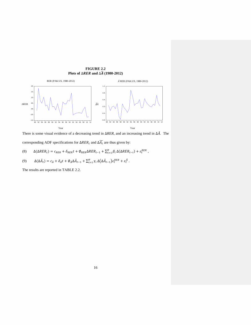
FIGURE 2.2

Plots of ∆𝑹𝑹𝑹𝑹𝑹𝑹 and ∆𝑨𝑨� (1980-2012)

RER (PAK:US, 1980-2012) �̃�𝐴 RER (PAK:US, 1980-2012)

ΔRER

𝛥𝛥𝐴𝐴�

Year Year There is some visual evidence of a decreasing trend in ∆RER, and an increasing trend in ∆�̃�𝐴. The

corresponding ADF specifications for ∆𝑅𝑅𝐸𝐸𝑅𝑅𝑡𝑡 and ∆𝐴𝐴𝑡𝑡� are thus given by:

(8) ∆(∆𝑅𝑅𝐸𝐸𝑅𝑅𝑡𝑡) = 𝑐𝑐𝑅𝑅𝐸𝐸𝑅𝑅 + 𝛿𝛿𝑅𝑅𝐸𝐸𝑅𝑅𝛾𝛾 + ∅𝑅𝑅𝐸𝐸𝑅𝑅∆𝑅𝑅𝐸𝐸𝑅𝑅𝑡𝑡−1 + ∑ 𝛽𝛽𝑖𝑖𝑝𝑝𝑖𝑖=1 ∆(∆𝑅𝑅𝐸𝐸𝑅𝑅𝑡𝑡−𝑖𝑖) + 𝜀𝜀𝑡𝑡𝑅𝑅𝐸𝐸𝑅𝑅 ,

(9) ∆(∆�̃�𝐴𝑡𝑡) = 𝑐𝑐𝐴𝐴� + 𝛿𝛿𝐴𝐴�𝛾𝛾 + ∅𝐴𝐴�∆�̃�𝐴𝑡𝑡−1 + ∑ 𝛾𝛾𝑖𝑖𝑝𝑝𝑖𝑖=1 ∆�∆�̃�𝐴𝑡𝑡−1�𝜀𝜀𝑡𝑡𝑅𝑅𝐸𝐸𝑅𝑅 + 𝜀𝜀𝑡𝑡𝐴𝐴

� .

The results are reported in TABLE 2.2.

-.10

-.05

.00

.05

.10

.15

.20

80 82 84 86 88 90 92 94 96 98 00 02 04 06 08 10 12

-0.8

-0.4

0.0

0.4

0.8

1.2

80 82 84 86 88 90 92 94 96 98 00 02 04 06 08 10 12

16

TABLE 2.2 ADF Test Statistics for ∆𝑹𝑹𝑹𝑹𝑹𝑹 and ∆𝑨𝑨�


Lag Length


Sample Statistic

5% Critical Value

∆RER Intercept + Trend 0 Yes -5.485 -3.568

∆�̃�𝐴 Intercept + Trend 1 Yes -4.329 -3.574


As before, I estimate the specifications with lags chosen by Eviews’ SIC selection

algorithm, and then test the residuals for white noise. For ∆RER, Eviews selects zero lags (p=0).

Applying the Ljung-Box Q-test to the resulting residuals produces the conclusion that the

residuals are white noise. For cumulative lags 1 to 10, the smallest p-value is 0.123 (for

cumulative lag 6). Hence, the ∆RER series is pretty clean and does not show evidence of serial

correlation.

For ∆�̃�𝐴, Eviews selects 5 lags. Using such a large number of lags will make us lose scarce

degrees of freedom greatly. As an alternative, I’ll start testing the series with 0 lags and will

successively add lags until the residuals become white noise.

With 1 lag i.e. (p=1 in ∑ 𝛽𝛽𝑖𝑖𝑝𝑝𝑖𝑖=1 ∆�̃�𝐴𝑡𝑡−𝑖𝑖), there remains no more evidence of presence of

serial correlation in ∆�̃�𝐴 series. . All of the p-values associated with the Ljung-Box Q-test are

greater than 5%, with the smallest p-value occurring at cumulative lag 9 (p-value = 0.144). Thus,

with one lag, the Ljung-Box Q-test fails to reject the null hypothesis of no serial correlation for all

cumulative lags up to 10.

17

I now run ADF unit root tests for ∆RER and ∆�̃�𝐴 with 0 and 1 lags, respectively. The

sample statistic for the ADF test of ∆RER is – 5.485. This is smaller than the 5% critical value of

-3.568. As a result, I reject the null hypothesis that ∆RER has a unit root. Thus ∆RER is first

differenced stationary. Similarly, the ADF unit root test for ∆�̃�𝐴 produces a sample statistic of -

4.329, which is smaller than the 5% critical value of -3.574. Based on this result, I fail to accept

the null that ∆�̃�𝐴 has a unit root. Putting all these results together, I conclude, on the basis of the

ADF tests, that the level series, RERt, and �̃�𝐴, are both I(1).

The Dickey-Fuller Generalized Least Squares (DF-GLS) Unit Root Test. The DF-GLS unit root

test is described in Elliot et al., 1996. Like the ADF test, DF-GLS test also follows the null

hypothesis of unit root. Following the ADF treatment above, I choose the “Intercept + Trend”

specification in the subsequent testing. TABLE 2.3 displays the DF-GLS unit root test results for

the 𝑅𝑅𝐸𝐸𝑅𝑅 and �̃�𝐴 series.

TABLE 2.3 DF-GLS Test Statistics for 𝑹𝑹𝑹𝑹𝑹𝑹 and 𝑨𝑨�


Lag Length


Sample Statistic

5% Critical Value

RER Intercept + Trend1 1 Yes -1.362 -3.190

�̃�𝐴 Intercept + Trend 1 Yes -1.685 -3.190

NOTE: Lag length is determined by automatic selection based on the SIC, subsequently adjusted to produce white noise in the residuals, if necessary. The sample statistics for the DF-GLS test of RER is – 1.362. This is greater than the 5% critical

value of -3.190. As a result, I fail to reject the null hypothesis that RER has a unit root. Similarly

1 DF-GLS has two specifications. In GLS de-trending the subject series is regressed on a constant and a linear trend and the resultant residual series is used in a standard DF regression. On the other hand, for GLS demeaning, the series is regressed on a drift term only and the resultant residuals series will be used in standard DF regression.

18

for �̃�𝐴, the ADF unit root test produces a sample statistic of -1.685, which is greater than its

corresponding 5% critical value. Based on this result, I also fail to reject the null that �̃�𝐴 has a unit

root.

Having determined that both series have unit roots, I next difference the two series and test

the status of their order of integration.

TABLE 2.4 DF-GLS Test Statistics for ∆𝑹𝑹𝑹𝑹𝑹𝑹 and ∆𝑨𝑨�


Lag Length


Sample Statistic

5% Critical Value

∆RER Intercept + Trend 0 Yes -5.160 -3.190

∆�̃�𝐴 Intercept + Trend 1 Yes -4.402 -3.190

NOTE: Lag length is determined by automatic selection based on the SIC, subsequently adjusted to produce white noise in the residuals, if necessary. The sample statistics for the DF-GLS test of ∆RER is – 5.160. This is substantially smaller than

the 5% critical value of -3.190. As a result, I reject the null hypothesis that ∆RER has a unit root.

Thus RER is first differenced stationary. For ∆�̃�𝐴, the automatic SIC lag selection procedure picks

5 lags. Based on my experience from the preceding ADF tests, I included only 1 lag for DF-GLS

estimation. The DF-GLS unit root test for ∆�̃�𝐴 produces a sample statistic of -4.402, which is

smaller than the 5% critical value of -3.190. Based on this result, I reject the null that ∆�̃�𝐴 has a

unit root. Putting all these results together, I conclude, on the basis of the DF-GLS tests, that the

level series, RER and �̃�𝐴, are both I(1), the same as my ADF test findings.

Elliott, Rothenberg and Stock (ERS) Point Optimal Test. The ERS point optimal test is described

in Elliot et al., 1996. Like the previous tests, the ERS test has the null of a unit root process.

19

Unlike previous tests, rejection of the null occurs when the sample statistic is smaller, not larger,

than the critical value. The test results for RER and �̃�𝐴 are given below.

TABLE 2.5 ERS Point Optimal Test Statistics for 𝑹𝑹𝑹𝑹𝑹𝑹 and 𝑨𝑨�


Lag Length


Sample Statistic

5% Critical Value

RER Intercept + Trend 0 Yes 57.524 5.720

�̃�𝐴 Intercept + Trend 0 Yes 50.200 5.720


For RER, the sample statistic value of 57.524 is substantially greater than the 5 percent

critical value of 5.724. Similarly for �̃�𝐴, the sample statistic is 50.200, which is greater than its 5

percent critical value. Thus, we are unable to reject our null of unit roots in levels for both 𝑅𝑅𝐸𝐸𝑅𝑅

and �̃�𝐴. Now let’s see, if the two series are difference stationary.

In TABLE 2.6, the sample statistics for ∆RER (7.925) is still greater than its corresponding

5 percent critical value. These results are not in line with our ADF and DF-GLS estimates, thus

making us to unable to reject our null once again and indicating the series to be greater than I(1).

For ∆�̃�𝐴, the sample statistics is 3.21 which is clearly less than its 5% critical value. Thus, for ∆�̃�𝐴,

we may reject our null hypothesis of unit root and thus conclude that 𝐴𝐴 � is I(1).

20

TABLE 2.6 ERS Point Optimal Test Statistics for ∆𝑹𝑹𝑹𝑹𝑹𝑹 and ∆𝑨𝑨�


Lag Length


Sample Statistic

5% Critical Value

∆RER Intercept + Trend 0 Yes 7.925 5.720

∆�̃�𝐴 Intercept + Trend 1 Yes 3.21 5.720


Now let’s test 𝑅𝑅𝐸𝐸𝑅𝑅 once again in order to see if the series is stationary when differenced

for a second time.

TABLE 2.7 ERS Point Optimal Test Statistics for ∆𝑹𝑹𝑹𝑹𝑹𝑹 against Successive Differences


Lag Length


Sample Statistic

5% Critical Value

∆2(∆𝑅𝑅𝐸𝐸𝑅𝑅) Intercept + Trend 0 Yes 17.89 5.720

∆3(∆𝑅𝑅𝐸𝐸𝑅𝑅) Intercept + Trend 0 Yes 17.91 5.72


The sample statistics reported against various orders of integration in TABLE 2.7 indicate that

RER is not stationary even up to the third order of integration. The P-statistic is substantially

higher than the 5 percent critical value at all levels of differencing. The ERS Point Optimal test

makes it hard to identify the exact order of integration of RER, in contrast with previous results

using the ADF and DF-GLS unit root tests..

21

The Kwiatkowski, Phillips, Schmidt and Shin (KPSS) Stationarity Test. The KPSS test is

described in Kwiatkowski et al., 1992. Unlike previous tests, the KPSS test has stationarity as the

null hypothesis, thus reversing the null and alternative hypotheses. The associated test results are

given below.

TABLE 2.8 KPSS Test Statistics for RER and 𝑨𝑨�


Lag Length


Sample Statistic

5% Critical Value

RER NA NA Yes 0.166 0.146

�̃�𝐴 NA NA Yes 0.169 0.146

NOTE: There is no option to choose lag length, so we just go with the default settings.

The results obtained for two series are exactly parallel to what we obtained from our ADF

and DF-GLS unit root tests. For RER, the sample LM-Statistic is. 0.166 which is greater than the 5

percent critical value of 0.146. In this case, greater LM-value means one rejects the null

hypothesis. Similarly for �̃�𝐴, the sample LM-Statistics of 0.169 is greater than the 5% critical

value, so that I reject the null of stationary for both 𝑅𝑅𝐸𝐸𝑅𝑅 and �̃�𝐴. Now let’s see, if the two series are

difference stationary or not.

The results obtained for the two series are pretty evident. For ∆RER, the sample LM-

Statistic of 0.074 is now smaller than the 5 percent critical value of 0.146. Thus, I am unable to

reject the null hypothesis of stationarity in ∆RER, something parallel with our previous unit root

results from ADF and DF-GLS tests. For �̃�𝐴, the sample LM-Statistic is 0.085, which is clearly

less than its 5 percent critical value. Hence, I fail to reject the null hypothesis of stationary in first

differences for ∆�̃�𝐴. So, conclusively, both RER and �̃�𝐴 are integrated of order 1, I(1).

22

TABLE 2.9 KPSS Test Statistics for ∆RER and ∆𝑨𝑨�


Lag Length


Sample Statistic

5% Critical Value

∆RER NA NA Yes 0.074 0.146

∆�̃�𝐴 NA NA Yes 0.085 0.146

NOTE: There is no option to choose lag length, so we just go with the default settings

Summary of unit root test results for 𝑅𝑅𝐸𝐸𝑅𝑅 and �̃�𝐴. In the previous sections, I tested the orders of

integration for RER and �̃�𝐴 by using four different stationarity tests. On employing these four tests,

I have well achieved the purpose of checking the robustness and consistency in my unit root tests

results. Except for ERS Point Optimal Test findings for RER, all the tests are proving RER and �̃�𝐴

to be first difference stationary. So, after a careful evaluation of the statistical evidences obtained

from all the tests, I regard the two series to be integrated of order one, I(1).

TABLE 2.10 the results I obtained using the various unit root tests. The last column of the

table states my conclusion about the stationary status of RER and �̃�𝐴 for Pakistan.

TABLE 2.10 Summary of Unit Root Test Results for 𝑹𝑹𝑹𝑹𝑹𝑹 and 𝑨𝑨�

Variable Order of integration as determined by:

Conclusion ADF DF-GLS ERS KPSS

𝑹𝑹𝑹𝑹𝑹𝑹 I(1) I(1) Indeterminate I(1) I(1)

𝑨𝑨� I(1) I(1) I(1) I(1) I(1)

23

Identification of the long-run relationship between RER and �̃�𝐴 against U.S. After obtaining

sufficient evidence in favor of RER and �̃�𝐴 being integrated of order one, I proceed towards

establishing whether a long-run cointegrating relationship exists between the two series.

Cointegration holds practical economic implications. While time series may be non-stationary in

levels, they may move together in the long run. A cointegrating relationship can also be

considered as a long term or equilibrium phenomenon where the subject variables diverge from

equilibrium in the short-run but maintain an association in the long-run.

There are several ways of identifying a cointegrating relationship between economic

series. I use a cointegration test that is embedded within a Vector Error Correction Model

(VECM). The test requires several steps.

STEP 1: Graph the suspected cointegrating series. It is clear from FIGURE 2.1 that both RER and

�̃�𝐴 have a definite time trend and both are upward trended. As noted above, this is consistent with

the BS hypothesis that an increase in �̃�𝐴 contributes to 𝑅𝑅𝐸𝐸𝑅𝑅 depreciation and vice versa. FIGURE

2.3 rescales the series and juxtaposes them. The successive divergence and convergence of the

two series is consistent with cointegrating behavior, although with a very slow speed of

adjustment.

FIGURE 2.3 Plots of 𝑹𝑹𝑹𝑹𝑹𝑹 and 𝑨𝑨� (1980-2012)

𝑨𝑨�

RER Year

3.2

3.4

3.6

3.8

4.0

4.2

4.4

7

8

9

10

11

12

13

80 82 84 86 88 90 92 94 96 98 00 02 04 06 08 10

24

STEP 2: Determining the lag length of the VECM specification. Before the cointegration test can

be carried out, it is necessary to specify the number of lags that will be used in the associated

VECM. To do that, I estimate a VAR model and use information criteria to select the appropriate

number of lags. The VECM will use this lag length minus one to account for the fact that it is

estimated in differences, not levels. Eviews provides a number of information criteria to assist in

the selection of lag length, including the Akaike information criterion (AIC), the Final Prediction

Error (FPE) criterion, the Schwarz Information Criterion (SC), and the Hannan-Quinn information

criterion (HQ). The results are reported below in TABLE 2.11.

Since 𝑅𝑅𝐸𝐸𝑅𝑅 and �̃�𝐴 series are taken on annual basis, the lag order selection is done from a

maximum of 4 lags in order to ensure good levels of adjustment in the model and for the

attainment of well behaved residuals. From TABLE 2.11, we may see that the four selection

criteria are unanimous in selecting 1 lag for the VAR model.

TABLE 2.11 Information Criteria Values for Different Lag Lengths

for the Multivariate VAR with 𝑹𝑹𝑹𝑹𝑹𝑹 and 𝑨𝑨�

Information Criterion Lag FPE AIC SC HQ

0 0.029 2.160 2.257 2.188

1 0.000* -2.189* -1.899* -2.106*

2 0.000 2.036 -1.552 -1.896

3 0.000 -1.985 -1.308 -1.790

4 0.000 -1.774 -0.903 -1.523

* Indicates lag order selected by the criterion FPE: Final prediction error AIC: Akaike information criterion SC: Schwarz information criterion HQ: Hannan-Quinn information criterion

25

Before proceeding to the identification of cointegrating vectors, I check whether the

residuals produced from the proposed VAR model are serially correlated. As I did for the unit

root testing, once again I’ll use the Ljung-Box Q-statistic to see if the proposed VAR model has

any issue of serial correlation. As proposed by two of our lag selection tests, on employing 1 lag

in the VAR model, I find that the resulting residuals are not consistent with white noise. The

smallest p-value is 0.027 and occurs at cumulative lag 6. So, in order to obtain white noise

residuals, I increase the number of lags until I get white noise in the residuals. The smallest p-

value with 4 lags is 0.064 and occurs at cumulative lag 8. This is indicative of the fact that we

must include 4 lags in our VAR specification. As a result, I will include 3 (= 4 - 1) lags in my

subsequent estimation of the VECM.

STEP 3: Deciding the specification of deterministic regressors. After determining the appropriate

lag length for my VECM specification, I look into exploring a cointegrating relationship between

𝑅𝑅𝐸𝐸𝑅𝑅 and �̃�𝐴. As I already have mentioned in the earlier sections of my study, I will employ VAR-

based cointegration tests using the methodology developed by Johansen (1991, 1995). The basic

advantages of this approach in comparison to Engle-Granger type single equation models is that

(i) the model does not necessitate the pre-discrimination between dependent and explanatory

variables (ii) it gives a definite solution to the problem of more than one cointegrating vector by

identifying the exact number of vectors and generates maximum likelihood estimates of identified

vectors. Besides, the approach allows testing the statistical significance of key variables.

The specification of deterministic regressors in the Johansen test is very important.

EViews allows the following 5 specifications of deterministic regressors:

Case 1: Assumes no deterministic trend in the data and no intercept or trend in the VAR and in

the cointegrating equation (CE)

26

Case 2: Assumes no deterministic trend in the data, but an intercept in the CE and no intercept in

VAR

Case 3: Assumes a linear deterministic trend in the data and an intercept in CE and test VAR

Case 4: Allows for a linear deterministic trend in data, intercept and trend in CE and no trend in

VAR

Case 5: allows for a quadratic deterministic trend in data, intercept and trend in CE and linear

trend in VAR.

I choose to use the specifications of cases 3 and 4 as the time series plots of the series indicate a

time trend.

STEP 4: Testing for the number of cointegrating vectors in the VECM. Eviews uses two tests, the

Trace and Maximum Eigenvalue tests, to determine whether the series are cointegrated and, if

they are, the number of cointegrating equations that exist.2 Given two series, there can either be

0, 1, or 2 cointegrating equations. A finding of 0 cointegrating vectors indicates that the series are

not cointegrated. A finding of 2 cointegrating vectors indicates that the series are stationary. A

finding of 1 cointegrating vector means that the series are non-stationary and cointegrated.

Eviews selects the number of cointegrating equations conditional on the specification of

deterministic regressors included in the error correction model (see Cases 1 through 5 above).

TABLE 2.12 reports the results of this analysis.

TABLE 2.12: Johansen Cointegration Rank Test Results

Test Case 1 Case 2 Case 3 Case 4 Case 5

Trace 0 0 0 0 0

Max Eigen 0 0 0 0 0

2 See Johansen and Juselius (1992) for details regarding these two tests.

27

Based on the time series plots for 𝑅𝑅𝐸𝐸𝑅𝑅 and �̃�𝐴, I decided that either Case 3 or Case 4 best

described the series. As it turns out, it doesn’t make a difference which case one chooses, because

the Trace and Maximum Eigenvalue tests conclude that the series are not cointegrated. Hence, we

cannot proceed with estimation of Vector Error Correction Model (VECM) for 𝑅𝑅𝐸𝐸𝑅𝑅 and �̃�𝐴 as

there is no significant statistical evidence in favor of a cointegrating relationship between two

series. I interpret this as evidence against the BS hypothesis.

Identification of the long-run relationship between RER and �̃�𝐴 against Japan and Korea. TABLE

1.2 above identified that Japan and Korea are also imporant trading partners of ASEAN member

states. Following Chinn (2000) and Thomas and King (2008), I next study Pakistan’s exchange

rate and productivity behavior against (i) Japan and (ii) Korea, respectively. While the U.S is a

commonly used benchmark, Japan and Korea may be more appropriate because of their

geographical immediacy with the Asian region. This should make traded goods arbitrage between

Pakistan and these trading partners more accurate. Once again, I will employ four unit root test

procedures in order to determine the order of integration of the RER and �̃�𝐴 series of Pakistan

against Japan and Korea. Afterwards, the Johansen Cointegration test procedure and the Vector

Error Correction Model (VECM) will be used to figure out the number of cointegrating vectors,

and the long-run elasticities between RER and �̃�𝐴, if applicable.

I being by plotting time series plots of the respective RER and �̃�𝐴 series, each calculated

with respect to Japan and Korea, rather than the U.S. For the sake of brevity, I only report the

juxtaposed series in FIGURE 2.4. This allows one to simultaneously identify trending behaviour,

as well as observed any crossings of the series that would indicate cointegration behaviour. By

design, the series are plotted so that they intersect at least once. Here, as well as throughout this

chapter, the solid line represents the RER series, while the dotted line represents �̃�𝐴.

28

FIGURE 2.4 Pakistan’s 𝑹𝑹𝑹𝑹𝑹𝑹 and 𝑨𝑨� against Japan and Korea

RER and �̃�𝐴 against Japan �̃�𝐴 RER and �̃�𝐴 against Korea �̃�𝐴

RER Year

RER Year

Unlike in the case with the U.S., the two series do not evidence a generally positive

relationship, as one would expect if the BS hypothesis were operative. Nor is there much visual

evidence to support an interpretation that deviations from the two series cause RER to adjust

towards some equilibrium value. Nevertheless, I proceed with formal testing. The results are

reported in TABLE 2.13 below.

TABLE 2.13

Unit Root Tests for PAK:Japan and PAK:Korea

Against Japan

Unit Root Tests Results Order of integration as determined by

Variable

𝑅𝑅𝐸𝐸𝑅𝑅

�̃�𝐴

ADF

I(1)

I(1)

DF-GLS

I(1)

I(1)

ERS

I(1)

Greater than I(1)

KPSS

I(1)

I(1)

Conclusion

I(1)

I(1)

Against Korea Unit Root Tests Results

Order of integration as determined by

Variable


�̃�𝐴

ADF

I(1)

Greater than I(1)

DF-GLS

I(1)

Greater than I(1)

ERS

Greater than I(1)

Greater than I(1)

KPSS

I(0)

I(0)

Conclusion

Indeterminate

Greater than I(1)

-1.8

-1.6

-1.4

-1.2

-1.0

-0.8

-0.6

-0.4

9.0

9.2

9.4

9.6

9.8

10.0

10.2

10.4

80 82 84 86 88 90 92 94 96 98 00 02 04 06 08 10

-2.2

-2.0

-1.8

-1.6

-1.4

-1.2

-1.0

-0.8

2.0

2.4

2.8

3.2

3.6

4.0

4.4

4.8

80 82 84 86 88 90 92 94 96 98 00 02 04 06 08 10 12

29

Starting with Japan, results from the four unit root tests3 show that RER is undisputedly

integrated of order one , I(1)4. I obtain similar results for �̃�𝐴 as well, except for the findings of the

ERS Point Optimal Test. However, considering the evidences from the majority of the tests, I

conclude that �̃�𝐴 is integrated of order one, I(1). Upon finding the two series eligible for

developing a cointegrating relationship, I tested them using the Johansen5 cointegration

procedure. As in the previous section, I judged Cases 3 and 4 to be best at describing the subject

series. The Trace and Maximum Eigenvalues of both cases indicated a rank of zero, suggesting

no cointegrating relationship between 𝑅𝑅𝐸𝐸𝑅𝑅 and �̃�𝐴. This is the same result I obtained in the

previous case using the U.S. Because the series are not cointegrated, there is no long-run

relationship between 𝑅𝑅𝐸𝐸𝑅𝑅 and �̃�𝐴. This supports the previous finding against the BS hypothesis.

Lastly, upon taking Korea as major trading partner of Pakistan, ADF and DF-GLS unit

root tests clearly state that country’s RER against Korea is first difference stationary. In contrast,

the ERS point Optimal test provides that the series has an order of integration greater than one;

while the KPPS test concludes that the series are I(0). With respect to �̃�𝐴, none of the four unit

root tests6 find that the series is I(1). Hence the two series are not eligible to be tested for the BS

effect because the series cannot be cointegrated.

3 The VAR specification of regression equations of our unit root tests, both for 𝑅𝑅𝐸𝐸𝑅𝑅 and �̃�𝐴, are robust to serial correlation. 4 The visual inspection of two series suggests inclusion of both a drift and a linear trend term in unit root regression equations. 5 Various lag order selection criteria suggested a VAR specification with 2 lags which is robust to serial correlation but not dynamically stable (even up to 6 lags). 6 The visual inspection of two series suggests inclusion of both a drift and a linear trend term in unit root regression equations.

30

III. COUNTRY STUDY: China

This section begins country-by-country reporting of results associated with testing the BS

hypothesis. The previous section on Pakistan provided a detailed report of the the many steps

involved in testing the BS hypothesis. The remainder of this chapter gives a much abbreviated

report for each country in the interests of brevity, starting with China. However, all of the steps

underlying my analysis are included in the EViews programs that are in the Appendix to this

chapter.

I begin by displaying time plots of RER and �̃�𝐴, where the exchange rates and productivity

differentials successively reference the U.S., Japan, and Korea. I only report one set of figures for

each reference country, with the solid line representing RER and the dotted line representing �̃�𝐴.

The left-hand scale reports the values of RER, and the right-hand scale reports the values of �̃�𝐴.

The graphs have been constructed such that the series intersect at least once.

FIGURE 3.1 China’s 𝑹𝑹𝑹𝑹𝑹𝑹 and 𝑨𝑨� against its Three Major Trading Partners

RER and �̃�𝐴 against US 𝑨𝑨� RER and �̃�𝐴 against Japan 𝑨𝑨�

RER Year

RER Year

0.2

0.3

0.4

0.5

0.6

0.7

0.8

0.9

1.0

2.0

2.5

3.0

3.5

4.0

4.5

5.0

5.5

6.0

80 82 84 86 88 90 92 94 96 98 00 02 04 06 08 10

-3.0

-2.9

-2.8

-2.7

-2.6

-2.5

-2.4

-2.3

-2.2

-2.1

8.6

8.8

9.0

9.2

9.4

9.6

9.8

10.0

10.2

10.4

80 82 84 86 88 90 92 94 96 98 00 02 04 06 08 10

31

RER and �̃�𝐴 against Korea 𝑨𝑨�

RER Year

Visual evidence consistent with the BS hypothesis is (i) both series trending in the same

direction, and (ii) RER adjusting to close the gap resulting from productivity differential shocks

that drive the series away from long-run equilibrium. The figures above provide weak evidence in

favour of the BS hypothesis. For example, the first graph, which uses the U.S. as the reference

country, shows both series trending upwards over time, with the RER series seemingly moving

downwards in the later years to close the gap between the two series. However, the speed of

adjustment is very slow.

I proceed with formal testing. First, the 𝑅𝑅𝐸𝐸𝑅𝑅 and �̃�𝐴 series will be tested though four tests

for unit roots. If the two series are concluded to be I(1), I will use the Johansen Cointegration

procedure to see if they are capable of establishing a long term cointegrating relationship. Upon

finding evidence of a cointegrating equation, I will estimate a Vector Error Correction Model

(VECM) to obtain an estimate of the long run BS coefficient. The results of my testing are

reported in TABLE 3.1 below.

The table is sectioned into three divisions, displaying China’s 𝑅𝑅𝐸𝐸𝑅𝑅 and �̃�𝐴 relationship

against the U.S, Japan and Korea. Against U.S, two out of four unit root tests (the ADF and DF-

GLS tests) indicate that China’s 𝑅𝑅𝐸𝐸𝑅𝑅 series is I(1). In contrast, the other two tests (the ERS Point

Optimal and KPSS tests) indicate an order of integration greater than one. With respect to �̃�𝐴, most

-2.6

-2.5

-2.4

-2.3

-2.2

-2.1

-2.0

-1.9

-1.8

-1.7

3.5

3.6

3.7

3.8

3.9

4.0

4.1

4.2

4.3

4.4

80 82 84 86 88 90 92 94 96 98 00 02 04 06 08 10

32

of the tests indicate that this series is I(0). As one of the series is concluded to have a unit root,

and the other series is stationary, the two series cannot be cointegrated. This constitutes evidence

against the BS hypothesis.

Upon taking Japan as China’s major trading partner, we obtain substantially different

results from our previous case. At least three out of four tests indicate that both 𝑅𝑅𝐸𝐸𝑅𝑅 and �̃�𝐴 series

of China are first-differenced stationary, I(1), making them eligible to be tested for a long-run

cointegrating relationship. However, when I use the Johansen Cointegration Test, I find that the

rank of the cointegrating matrix is zero for all five cases. This is evidence that the BS effect

doesn’t hold for China when that country’s major trading partner is Japan.

Lastly, taking Korea as China’s major trading partner, for country’s 𝑅𝑅𝐸𝐸𝑅𝑅, I obtain results

similar to the first case where China’s major trading partner was the U.S. The results from the

respective unit root tests are mixed, indicated that the series is level stationary, first-difference

stationarity, or more than first-difference stationary. This leaves me uncertain about the actual

order of integration of the series. On the contrary, for 𝐴𝐴,� the majority of the tests point to the series

being level stationary. Given the different orders of integration for the two series, I terminate my

testing for cointegration. On the basis of all my tests, I conclude that the BS hypothesis does not

hold for China.

33

TABLE 3.1 Summary of Test Results for China

Against U.S


Variable 𝑅𝑅𝐸𝐸𝑅𝑅 �̃�𝐴

ADF I(1) I(0)

DF-GLS I(1) I(0)

ERS Greater than I(1) Greater than I(1)

KPSS Greater than I(1) I(0)

Conclusion Indeterminate

I(0)

Against Japan Unit Root Tests Results

Order of integration as determined by Variable 𝑅𝑅𝐸𝐸𝑅𝑅 �̃�𝐴

ADF I(1) I(1)

DF-GLS I(1) I(1)

ERS I(1)

Greater than I(1)

KPSS I(0) I(1)

Conclusion I(1) I(1)

Johansen Cointegration Test Results

Test Specifications and No. of Cointegrating Vectors Test

Trace Max Eigen

Case 1 0 0

Case 2 0 0

Case 3 0 0

Case 4 0 0

Case 5 0 0



Variable 𝑅𝑅𝐸𝐸𝑅𝑅 �̃�𝐴

ADF I(1) I(0)

DF-GLS I(1) I(0)

ERS Greater than I(1) Greater than I(1)

KPSS I(0) I(0)

Conclusion Indeterminate

I(0)

IV. COUNTRY STUDY: Japan

For Japan, we first inspect the 𝑅𝑅𝐸𝐸𝑅𝑅 and �̃�𝐴 series visually. Both against the U.S and Korea,

the two plots displayed in FIGURE 4.1 indicate that (i) over certain years (though not over all

years) 𝑅𝑅𝐸𝐸𝑅𝑅 and �̃�𝐴 trend in the same direction, and (ii) the 𝑅𝑅𝐸𝐸𝑅𝑅 series shows some evidence of

trying to adjust the long run disequilibrium caused by sectoral productivity gaps. On the whole,

34

the visual examination of the behavior of 𝑅𝑅𝐸𝐸𝑅𝑅 and �̃�𝐴 series provides some evidence in favor of

BS hypothesis for Japan. I proceed with testing.

FIGURE 4.1 Japan’s 𝑹𝑹𝑹𝑹𝑹𝑹 and 𝑨𝑨� against its Two Major Trading Partners

RER and �̃�𝐴 against US 𝑨𝑨� RER and �̃�𝐴 against Korea 𝑨𝑨�

RER Year

RER Year

TABLE 4.1 displays the unit root and cointegration tests statistics for Japan against its two

trading partners. Against the U.S, we see that all the four unit root test statistics are indicating the

RER series to be first-difference stationarity. However, for �̃�𝐴, I obtain a mix of statistical

evidences from the four stationarity tests. The results alternatively indicate that �̃�𝐴 is level

stationary, first-difference stationarity, or integrated of order greater than one. Due to the

undesirable behavior of �̃�𝐴, the two series cannot be tested for developing a cointegrating

relationship.

Turning now to Korea as Japan’s major trading partner, I once again come up with

indeterminate results for the two series. The order of integration for RER is unclear when focused

on Korea as Japan’s trading partner. The respective unit root tests give different orders of

integration. However, all four tests unanimously indicate �̃�𝐴 to be integrated of order one, I(1).

Thus, similar to the case against U.S, Japan’s 𝑅𝑅𝐸𝐸𝑅𝑅 and �̃�𝐴 against Korea mutually do not

statistically qualify to be tested for cointegration. Putting together all the preceding results, I

conclude that the BS hypothesis does not hold for Japan.

4.2

4.3

4.4

4.5

4.6

4.7

4.8

4.9

5.0

5.1

6

7

8

9

10

11

12

13

14

15

80 82 84 86 88 90 92 94 96 98 00 02 04 06 08 10

-2.7

-2.6

-2.5

-2.4

-2.3

-2.2

-2.1

-2.0

-1.9

-1.8

7.0

7.5

8.0

8.5

9.0

9.5

10.0

10.5

11.0

11.5

80 82 84 86 88 90 92 94 96 98 00 02 04 06 08 10

35

TABLE 4.1 Summary of Test Results for Japan

Against U.S


Variable


�̃�𝐴

ADF

I(1)

I(0)

DF-GLS

I(1)

I(1)

ERS

I(1)*

Greater than I(1)

KPSS

I(1)

I(1)

Conclusion

I(1)

Indeterminate

Against Korea


Variable


�̃�𝐴

ADF

I(1)

I(1)

DF-GLS

I(1)

I(1)

ERS

I(0)

I(1)*

KPSS

Greater than I(1)

I(1)

Conclusion

Indeterminate

I(1)

V. COUNTRY STUDY: Korea

Firstly, in FIGURE 5.1, the visual examination of 𝑅𝑅𝐸𝐸𝑅𝑅 and �̃�𝐴 series of Korea against the

U.S and Japan shows that (i) Over the entire sample period, 𝑅𝑅𝐸𝐸𝑅𝑅 and �̃�𝐴 are sharing a common

trend, and (ii) the 𝑅𝑅𝐸𝐸𝑅𝑅 series shows considerable evidence of trying to adjust the long run

disequilibrium caused by sectoral productivity gaps in case where Korea’s major trading partner is

Japan. Nevertheless, it is less often against the U.S. On the whole, the visual examination of the

behavior of 𝑅𝑅𝐸𝐸𝑅𝑅 and �̃�𝐴 series provides enough support to test Korea for BS hypothesis.

36

FIGURE 5.1 Korea’s 𝑹𝑹𝑹𝑹𝑹𝑹 and 𝑨𝑨� against its Two Major Trading Partners


RER Year

RER Year

TABLE 5.1 reports Korea’s result against U.S and Japan. The order of integration of

country’s 𝑅𝑅𝐸𝐸𝑅𝑅 against U.S is difficult to determine as ADF and DF-GLS tests are showing the

series to be first-difference stationary whereas the other two tests are favoring the series to be

stationary in levels. Nevertheless, all the tests are collectively showing country’s sectoral

productivity differential against U.S. i.e. �̃�𝐴 to be integrated of order one, I(1). But, being

inconclusive about the stationarity status of 𝑅𝑅𝐸𝐸𝑅𝑅, I cannot proceed further with testing the

cointegrating relationship between the two series.

Now coming towards Japan as Korea’s largest trading partner, the country’s situation is no

different from the preceding case. I am once again imprecise about the correct order of integration

for 𝑅𝑅𝐸𝐸𝑅𝑅. So as a consequence, I am unable to test country’s 𝑅𝑅𝐸𝐸𝑅𝑅 and �̃�𝐴 against BS hypothesis.

However, all the four tests are mutually displaying �̃�𝐴 to be differenced stationary. Based upon my

statistical findings, I say that Korea is not eligible to be tested for BS effect, both against the U.S

and Japan.

6.7

6.8

6.9

7.0

7.1

7.2

7.3

7.4

6

7

8

9

10

11

12

13

80 82 84 86 88 90 92 94 96 98 00 02 04 06 08 10

1.8

1.9

2.0

2.1

2.2

2.3

2.4

2.5

2.6

2.7

7.0

7.5

8.0

8.5

9.0

9.5

10.0

10.5

11.0

11.5

80 82 84 86 88 90 92 94 96 98 00 02 04 06 08 10

37

TABLE 5.1 Summary of Test Results for Korea

Against U.S

Unit Root Tests Results


Variable


�̃�𝐴

ADF

I(1)

I(1)

DF-GLS

I(1)

I(1)

ERS

I(0)

I(1)

KPSS

I(0)

I(0)

Conclusion

Indeterminate

I(1)

Against Japan


Variable


�̃�𝐴

ADF

I(1)

I(1)

DF-GLS

I(1)

I(1)

ERS

I(0)

I(1)*

KPSS

Greater than I(1)

I(1)

Conclusion

Indeterminate

I(1)

VI. COUNTRY STUDY: Singapore

Starting with the visual assessment, in FIGURE 6.1 Singapore comes up with even lesser

evidence in favor of BS hypothesis in comparison to its earlier discussed regional member

economies. Against its three major trading partners, the graphical analysis of 𝑅𝑅𝐸𝐸𝑅𝑅 and �̃�𝐴 reveals

that from the Year 1980-2000, Singapore’s RER and �̃�𝐴 against the U.S are exhibiting opposite

trends. But, the two series seem to be following a positive trend since year 2000 onwards.

However, against Japan and Korea, 𝑅𝑅𝐸𝐸𝑅𝑅 and �̃�𝐴 pursue very much common trend over the entire

sample period. On the average, the situation is quite convincing for testing the country for BS

hypothesis.

38

FIGURE 6.1 Singapore’s 𝑹𝑹𝑹𝑹𝑹𝑹 and 𝑨𝑨� against its Three Major Trading Partners


RER Year RER Year


RER Year TABLE 6.1 displays Singapore’s results against the U.S, Japan and Korea. Against the

U.S, it is evident from three out of four unit root tests that Singapore’s 𝑅𝑅𝐸𝐸𝑅𝑅 is stationary in levels,

a situation not compliant with Cointegration test procedure. For �̃�𝐴, I am indefinite about the right

order of stationarity since I am getting a mix of results from our four unit root tests.

Upon taking Japan as Singapore’s major trading partner, I obtain substantially different

results from previous case. Though, not all four, but at least three out of four tests are proving

both 𝑅𝑅𝐸𝐸𝑅𝑅 and �̃�𝐴 series of Singapore to be first-difference stationary, I(1). After qualifying to be

tested for long run cointegrating relationship with each other, at second stage I test the two series

for Johansen Cointegration Test procedure. As anticipated from the visual analysis, I obtain a rank

0.2

0.3

0.4

0.5

0.6

0.7

0.8

0.9

1.0

9.6

10.0

10.4

10.8

11.2

11.6

12.0

12.4

12.8

80 82 84 86 88 90 92 94 96 98 00 02 04 06 08 10

-4.8

-4.6

-4.4

-4.2

-4.0

-3.8

-3.6

-3.4

-3.2

4

5

6

7

8

9

10

11

12

80 82 84 86 88 90 92 94 96 98 00 02 04 06 08 10

-7.0

-6.8

-6.6

-6.4

-6.2

-6.0

-5.8

6

7

8

9

10

11

12

80 82 84 86 88 90 92 94 96 98 00 02 04 06 08 10

Commented [BR1]: You are inserting extra spaces between paragraphs. Please set the paragraph parameters so that the line spacing between paragraphs is the same as the line spacing within paragraphs. If you do not know how to do this, let me konw.

39

of zero against all of Johansen’s five cases proving the fact that despite of being first-difference

stationary, �̃�𝐴 have no good tendency of explaining the long run dynamics of Singapore’s RER.

TABLE 6.1 Summary of Test Results for Singapore

Against U.S


Variable


�̃�𝐴

ADF

Greater than I(1)

I(1)

DF-GLS

I(0)

I(1)

ERS

I(0)

Greater than I(1)

KPSS

I(0)

I(0)

Conclusion

I(0)

Indeterminate

Against Japan


Variable


�̃�𝐴

ADF

I(1)

I(1)

DF-GLS

I(1)

I(1)

ERS

I(1)

I(1)*

KPSS

I(0)

I(0)

Conclusion

I(1)

I(1)


Test Specifications and No. of Cointegrating Vectors

Test

Trace

Max Eigen

Case 1

0

0

Case 2

0

0

Case 3

0

0

Case 4

0

0

Case 5

0

0

Against Korea


Variable


�̃�𝐴

ADF

I(1)

I(1)

DF-GLS

I(1)

I(0)

ERS

I(1)*

Greater than I(1)

KPSS

I(0)

I(0)

Conclusion

I(1)

Indeterminate

40

Against Korea, I am once again unable to test country’s 𝑅𝑅𝐸𝐸𝑅𝑅 and �̃�𝐴 for BS hypothesis.

Though 𝑅𝑅𝐸𝐸𝑅𝑅′𝑠𝑠 order of integration is one, I(1), I am indeterminate about the exact level of

stationarity of �̃�𝐴 as I get varying results from the four stationarity tests. Conclusively, BS effect

does not hold for Singapore against any of its three largest trading partners.

VII. COUNTRY STUDY: Malaysia

FIGURE 7.1 demonstrates Malaysian 𝑅𝑅𝐸𝐸𝑅𝑅 and �̃�𝐴 behavior against the U.S, Japan and

Korea. The plots provided in the figure represent that (i) the two series are crossing each other

quite frequently (from 1980-94 against U.S and Japan and till 2000 against Korea) which is

indicative of their good potential of establishing a long run cointegrating relationship with each

other, and (ii) throughout the sample period, the two series are following the same common trend,

specifically for the case where Malaysia’s major trading partner is Korea. These conduct of 𝑅𝑅𝐸𝐸𝑅𝑅

and �̃�𝐴 are very illuminating in a sense that they signify the possibility of presence of BS effect for

Malaysia.

FIGURE 7.1 Malaysia’s 𝑹𝑹𝑹𝑹𝑹𝑹 and 𝑨𝑨� against its Three Major Trading Partners


RER Year

RER Year

0.6

0.7

0.8

0.9

1.0

1.1

1.2

1.3

1.4

9.0

9.5

10.0

10.5

11.0

11.5

12.0

12.5

13.0

80 82 84 86 88 90 92 94 96 98 00 02 04 06 08 10

-4.4

-4.2

-4.0

-3.8

-3.6

-3.4

-3.2

8.8

9.2

9.6

10.

10.

10.

11.

80 82 84 86 88 90 92 94 96 98 00 02 04 06 08 10

41


RER Year

By looking into TABLE 7.1, I can see Malaysia’s results against its three trading partners

in the context of BS effect. Starting with U.S as Malaysia’s largest trading partner, for 𝑅𝑅𝐸𝐸𝑅𝑅, all

the four unit root tests are commonly recommending the series to be first-difference stationary.

However, for �̃�𝐴, I am getting ambiguous results as all the four unit root tests are displaying

contradictory results. Due to this uncertainty, Malaysia is not eligible to be tested for BS

hypothesis when U.S is country’s major trading partner.

Now, when Japan is Malaysia’s major trading partner, the statistical evidences obtained

from all of four unit root tests show that �̃�𝐴 is undisputedly integrated of order one , I(1). I obtain

pretty same results for 𝑅𝑅𝐸𝐸𝑅𝑅 as well, except for the findings of ERS Point Optimal Test which

proves the series with order of integration greater than one. However, taking into consideration

the evidences from majority of the tests, I treat 𝑅𝑅𝐸𝐸𝑅𝑅 to be integrated of order one, I(1). Upon

finding the two series eligible for developing a cointegrating relationship, I tested them for

Johansen cointegration procedure. The Trace and Maximum Eigen values of both cases are

suggesting no cointegrating relationship between 𝑅𝑅𝐸𝐸𝑅𝑅 and �̃�𝐴, yielding a rank of zero. Hence, I

cannot proceed with estimation of Vector Error Correction Model (VECM) for 𝑅𝑅𝐸𝐸𝑅𝑅 and �̃�𝐴 as

-6.3

-6.2

-6.1

-6.0

-5.9

-5.8

-5.7

-5.6

-5.5

8.8

9.2

9.6

10.0

10.4

10.8

11.2

11.6

12.0

80 82 84 86 88 90 92 94 96 98 00 02 04 06 08 10

42

there is no significant statistical evidence in favor of a cointegrating relationship between two

series.

TABLE 7.1 Summary of Test Results for Malaysia

Against U.S


Variable


�̃�𝐴

ADF

I(1)

I(1)

DF-GLS

I(1)

I(0)

ERS

I(1)*

I(1)

KPSS

I(0)

I(0)

Conclusion

I(1)

Indeterminate

Against Japan


Variable


�̃�𝐴

ADF

I(1)

I(1)

DF-GLS

I(1)

I(1)

ERS

I(1)

I(1)

KPSS

Greater than I(1)

I(1)

Conclusion

I(1)

I(1)


Test Specifications and No. of Cointegrating Vectors

Test

Trace

Max Eigen

Case 1

0

0

Case 2

0

0

Case 3

0

0

Case 4

0

0

Case 5

0

0

Against Korea

Unit Root Tests Results


Variable


�̃�𝐴

ADF

I(1)*

I(1)

DF-GLS

I(1)

I(1)

ERS

I(0)

I(1)

KPSS

I(0)

I(1)

Conclusion

Indeterminate

I(1)

43

Lastly, taking Korea as Malaysia’s major trading partner, for country’s 𝑅𝑅𝐸𝐸𝑅𝑅, I am

obtaining a blend of statistical evidences from four stationarity tests, displaying the series to be

level stationary as well as first-difference stationarity thus leaving me uncertain about the actual

order of integration of the series. On contrary, for 𝐴𝐴,� all of the tests advocate the series to be

differenced stationary. Hence, the present situation once again prevents me to test two series for

establishing any possible long run cointegrating relationship. Thus, convincingly, like all the prior

cases, BS hypothesis does not hold for Malaysia as well.

VIII. COUNTRY STUDY: Thailand

Figure 8.1 contains three plots for Thailand against its major trading partners. From the

graphical view, it is very much obvious that (i) except for the U.S, country’s 𝑅𝑅𝐸𝐸𝑅𝑅 and �̃�𝐴 series are

crossing each other time and again which makes it plausible that BS hypothesis could hold for

Thailand against Japan and Korea, and (ii) Almost for the entire sample period, two series are co-

moving in the same direction thus sharing a common trend. These data characteristics provide me

with an adequate rationale to proceed with the formal tests of cointegration.

FIGURE 8.1 Thailand’s 𝑹𝑹𝑹𝑹𝑹𝑹 and 𝑨𝑨� against its Three Major Trading Partners


RER Year

RER Year

3.1

3.2

3.3

3.4

3.5

3.6

3.7

3.8

7

8

9

10

11

12

13

14

80 82 84 86 88 90 92 94 96 98 00 02 04 06 08 10

-2.0

-1.8

-1.6

-1.4

-1.2

-1.0

-0.8

-0.6

4

5

6

7

8

9

10

11

80 82 84 86 88 90 92 94 96 98 00 02 04 06 08 10

44


RER Year

TABLE 8.1 is displaying Thailand’s results. When country’s largest trading partner is U.S,

all of the four unit root tests are collectively showing 𝑅𝑅𝐸𝐸𝑅𝑅 to be first-difference stationary.

However, the results for �̃�𝐴 are altogether contradictory. All the unit root tests are verifying the

series to be stationary in levels, something which stops me from testing the country for BS

hypothesis.

Against Japan, I obtain substantially good evidence in favor of both 𝑅𝑅𝐸𝐸𝑅𝑅 and �̃�𝐴 to be

integrated of order one. But when I tried to establish a long run cointegrating relationship between

the two series, I obtain zero rank against all the five cases of Johansen cointegration test. Hence,

despite of being non-stationary in levels, the two series don’t cointegrate with each other thus

refuting BS hypothesis for Thailand.

, against Korea, similar to all of our previously discussed cases, Thailand 𝑅𝑅𝐸𝐸𝑅𝑅 and �̃�𝐴

together don’t qualify to develop a long run cointegrating relationship. Though I obtain

sufficiently strong evidence in favor of 𝑅𝑅𝐸𝐸𝑅𝑅 to be stationary in first-differences, the stationarity

status of �̃�𝐴 is unclear as I am obtaining conflicting results from our unit root tests. In nutshell, BS

hypothesis is not validated for Thailand.

-4.0

-3.9

-3.8

-3.7

-3.6

-3.5

-3.4

-3.3

-3.2

-3.1

-3.0

6.8

7.2

7.6

8.0

8.4

8.8

9.2

9.6

10.0

10.4

10.8

80 82 84 86 88 90 92 94 96 98 00 02 04 06 08 10

45

TABLE 8.1

Summary of Test Results for Thailand

Against U.S Unit Root Tests Results


Variable


�̃�𝐴

ADF

I(1)

I(0)

DF-GLS

I(1)

I(0)

ERS

I(1)*

I(0)

KPSS

I(0)

I(0)

Conclusion

I(1)

I(0)



Variable


�̃�𝐴

ADF

I(1)

I(1)

DF-GLS

I(1)

I(1)

ERS

I(1)*

I(1)

KPSS

Greater than I(1)

I(0)

Conclusion

I(1)

I(1)

Johansen Cointegration Test Results Test Specifications and No. of Cointegrating Vectors

Test

Trace

Max Eigen

Case 1

0

0

Case 2

0

0

Case 3

0

0

Case 4

0

0

Case 5

0

0



Variable


�̃�𝐴

ADF

I(1)

I(1)

DF-GLS

I(1)

I(1)

ERS

I(1)*

Greater than I(1)

KPSS

I(0)

I(0)

Conclusion

I(1)

Indeterminate

IX. COUNTRY STUDY: Philippines

In FIGURE 9.1, from the visual assessment of Philippines, we get substantially lesser

evidence in favor of BS hypothesis in comparison to its earlier discussed regional member

46

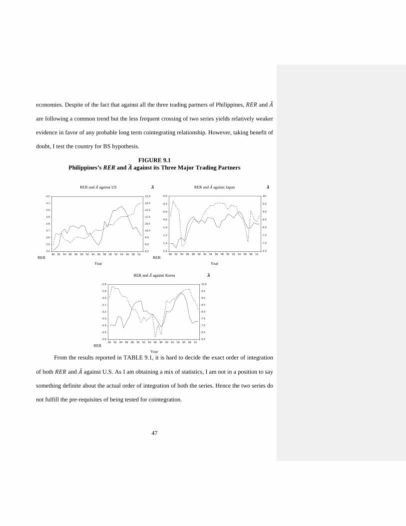
economies. Despite of the fact that against all the three trading partners of Philippines, 𝑅𝑅𝐸𝐸𝑅𝑅 and �̃�𝐴

are following a common trend but the less frequent crossing of two series yields relatively weaker

evidence in favor of any probable long term cointegrating relationship. However, taking benefit of

doubt, I test the country for BS hypothesis.

FIGURE 9.1 Philippines’s 𝑹𝑹𝑹𝑹𝑹𝑹 and 𝑨𝑨� against its Three Major Trading Partners


RER Year

RER Year


RER Year

From the results reported in TABLE 9.1, it is hard to decide the exact order of integration

of both 𝑅𝑅𝐸𝐸𝑅𝑅 and �̃�𝐴 against U.S. As I am obtaining a mix of statistics, I am not in a position to say

something definite about the actual order of integration of both the series. Hence the two series do

not fulfill the pre-requisites of being tested for cointegration.

3.4

3.5

3.6

3.7

3.8

3.9

4.0

4.1

4.2

8.5

9.0

9.5

10.0

10.5

11.0

11.5

12.0

12.5

80 82 84 86 88 90 92 94 96 98 00 02 04 06 08 10

-1.6

-1.4

-1.2

-1.0

-0.8

-0.6

-0.4

-0.2

6.5

7.0

7.5

8.0

8.5

9.0

9.5

10.0

80 82 84 86 88 90 92 94 96 98 00 02 04 06 08 10

-3.6

-3.5

-3.4

-3.3

-3.2

-3.1

-3.0

-2.9

-2.8

6.0

6.5

7.0

7.5

8.0

8.5

9.0

9.5

10.0

80 82 84 86 88 90 92 94 96 98 00 02 04 06 08 10

47

But against Japan, both 𝑅𝑅𝐸𝐸𝑅𝑅 and �̃�𝐴 of Philippines are integrated of order one. However,

when I tested the two series if they make any long run cointegrating relationship with each other, I

obtain a rank of zero representing the fact that despite of being non-stationary in levels the two

series are not cointegrating thus failing to explain BS hypothesis for Philippines.

Similar to the case against U.S, Philippines is unable to establish a long run relationship

between 𝑅𝑅𝐸𝐸𝑅𝑅 and �̃�𝐴 against Korea as well because 𝑅𝑅𝐸𝐸𝑅𝑅 is stationary in levels, something in

conflict with eligibility for cointegration. Though, it is evident from majority of the unit root tests

that �̃�𝐴 is stationary in first-differences, due to undesirable order of stationarity of RER, I cannot

proceed with establishing a cointegrating relationship between two series. Thus, similar to its

earlier discussed regional economies, Philippines does not seem to hold BS effect against any of

its three prominent trading partners.

48

TABLE 9.1

Summary of Test Results for Philippines

Against U.S


Variable


�̃�𝐴

ADF

I(0)

I(1)

DF-GLS

I(1)

I(1)

ERS

I(1)*

Greater than I(1)

KPSS

I(0)

Greater than I(1)

Conclusion

Indeterminate

Indeterminate

Against Japan


Variable


�̃�𝐴

ADF

I(1)

I(1)

DF-GLS

I(1)

I(1)

ERS

I(1)*

Greater than I(1)

KPSS

I(1)

I(1)

Conclusion

I(1)

I(1)

Johansen Cointegration Test Results Test Specifications and No. of Cointegrating Vectors

Test

Trace

Max Eigen

Case 1

0

0

Case 2

0

0

Case 3

2

0

Case 4

0

0

Case 5

0

0

Against Korea


Variable


�̃�𝐴

ADF

I(0)

I(1)

DF-GLS

I(0)

I(1)

ERS

Greater than I(1)

Greater than I(1)

KPSS

I(0)

I(1)

Conclusion

I(0)

I(1)

49

X. COUNTRY STUDY: Bangladesh

As I already have discussed Pakistan from South Asia, coming towards Bangladesh as

another important participant of SAARC agreement, the country’s real exchange rate and sectoral

productivity gaps with the U.S, Japan and Korea are given in FIGURE 10.1. It is very much

visible from the figure that (i) against all the three trading partners, Bangladesh’s 𝑅𝑅𝐸𝐸𝑅𝑅 and �̃�𝐴 are

not co-moving in a common direction, and (ii) the two series are rarely crossing each other. Both

of these characteristics leave me with little evidence in favor of BS hypothesis. Nevertheless,

visual inspection being an inadequate verification, I will test two series for a possible

cointegrating relationship, if any exists.

FIGURE 10.1 Bangladesh’s 𝑹𝑹𝑹𝑹𝑹𝑹 and 𝑨𝑨� against its Three Major Trading Partners


RER Year

RER Year


RER Year

3.80

3.85

3.90

3.95

4.00

4.05

4.10

4.15

4.20

4.25

5

6

7

8

9

10

11

12

13

14

80 82 84 86 88 90 92 94 96 98 00 02 04 06 08 10

-.9

-.8

-.7

-.6

-.5

-.4

-.3

-.2

-.1

6.5

7.0

7.5

8.0

8.5

9.0

9.5

10.0

10.5

80 82 84 86 88 90 92 94 96 98 00 02 04 06 08 10

-3.4

-3.3

-3.2

-3.1

-3.0

-2.9

-2.8

-2.7

-2.6

-2.5

-2.4

6.8

7.2

7.6

8.0

8.4

8.8

9.2

9.6

10.0

10.4

10.8

80 82 84 86 88 90 92 94 96 98 00 02 04 06 08 10

50

In TABLE 10.1, I have given unit root and cointegration tests results for Bangladesh

against its largest trading partners. Against U.S, I am unable to test country for BS hypothesis

because of disagreeable stationarity orders of 𝑅𝑅𝐸𝐸𝑅𝑅 and �̃�𝐴. I am unable to determine the correct

order of integration of 𝑅𝑅𝐸𝐸𝑅𝑅 because the four unit root tests are providing me with conflicting

stationarity levels. On the other hand, majority of the unit root tests are displaying an inclination

towards level stationarity when it comes to decide the order of integration of �̃�𝐴. Hence the two

series are not eligible to be used for establishing a long run cointegrating relationship.

Similarly against Japan, once again Bangladesh cannot be tested for BS hypothesis. Though

country’s RER against Japan is first-difference stationary, the country’s sectoral productivity

differential with Japan i.e. �̃�𝐴 is stationary in levels, preventing me to employ two series for

Johansen Cointegration Test procedure.

Like the preceding two cases, once again, against Korea, I am obtaining disagreeable order

of integration for �̃�𝐴 i.e. the series is level stationary. Though 𝑅𝑅𝐸𝐸𝑅𝑅 is first-difference stationary, we

are not in a position to test Bangladesh for BS hypothesis because of undesirable stationarity

behavior of �̃�𝐴. Hence, BS hypothesis fails for Bangladesh as I remained unable to find any log run

cointegrating relationship between 𝑅𝑅𝐸𝐸𝑅𝑅 and �̃�𝐴 against any of country’s largest trading partners.

51

TABLE 10.1

Summary of Test Results for Bangladesh

Against U.S Unit Root Tests Results


Variable


�̃�𝐴

ADF

I(1)*

I(0)

DF-GLS

I(1)

I(0)

ERS

Greater than I(1)

Greater than I(1)

KPSS

I(0)

I(0)

Conclusion

Indeterminate

I(0)



Variable


�̃�𝐴

ADF

I(1)

I(0)

DF-GLS

I(1)

I(0)

ERS

I(1)

I(0)

KPSS

I(0)

Greater than I(1)

Conclusion

I(1)

I(0)



Variable


�̃�𝐴

ADF

I(1)

I(0)

DF-GLS

I(1)

I(0)

ERS

I(1)

I(0)

KPSS

I(0)

I(0)

Conclusion

I(1)

I(0)

XI. COUNTRY STUDY: Sri Lanka

From Figure 11.1, the visual examination of 𝑅𝑅𝐸𝐸𝑅𝑅 and �̃�𝐴 series of country against the U.S,

Japan and Korea shows that (i) Over the entire sample period, 𝑅𝑅𝐸𝐸𝑅𝑅 and �̃�𝐴 are rarely sharing a

common trend, and (ii) Against all three trading partners, the 𝑅𝑅𝐸𝐸𝑅𝑅 series does not show any

substantial evidence of trying to adjust the long run disequilibrium caused by sectoral productivity

gaps as the two series are seldom crossing each over the entire sample period. On the whole, the

52

visual examination of the two series does not give us enough hope that country’s RER may be

affected by BS effect.

FIGURE 11.1 Sri Lanka’s 𝑹𝑹𝑹𝑹𝑹𝑹 and 𝑨𝑨� against its Three Major Trading Partners


RER Year

RER Year


RER Year

The country results are given in TABLE 11.1. Country’s RER and �̃�𝐴 and against U.S are

hard to determine, if they are difference stationary or not. This uncertainty is making me

indeterminate about the accurate order of integration of two series.

Similar is the situation against Japan. A mix of statistical evidences from four unit root

tests are preventing me to say something determinedly about the order of integration of RER and

�̃�𝐴. Hence, I declare the status of two series as indeterminate and thus unable to test them in the

context of BS hypothesis for Sri Lanka where country’s major trading partner is Japan.

4.2

4.3

4.4

4.5

4.6

4.7

4.8

7

8

9

10

11

12

13

90 92 94 96 98 00 02 04 06 08 10

-.4

-.3

-.2

-.1

.0

.1

.2

.3

.4

8.6

8.8

9.0

9.2

9.4

9.6

9.8

10.0

10.2

90 92 94 96 98 00 02 04 06 08 10

-2.8

-2.7

-2.6

-2.5

-2.4

-2.3

-2.2

-2.1

4

5

6

7

8

9

10

11

90 92 94 96 98 00 02 04 06 08 10

53

TABLE 11.1

Summary of Test Results for Sri Lanka

Against U.S


Variable


�̃�𝐴

ADF

I(1)

I(1)

DF-GLS

I(1)

I(1)

ERS

Greater than I(1)

Greater than I(1)

KPSS

I(0)

I(0)

Conclusion

Indeterminate

Indeterminate

Against Japan


Variable


�̃�𝐴

ADF

I(1)

I(0)

DF-GLS

I(0)

I(0)

ERS

I(1)

Greater than I(1)

KPSS

I(0)

I(1)*

Conclusion

Indeterminate

Indeterminate

Against Korea


Variable


�̃�𝐴

ADF

I(1)

I(0)

DF-GLS

I(1)

I(1)

ERS

Greater than I(1)

I(1)

KPSS

I(0)

I(1)*

Conclusion

Indeterminate

I(1)

Note: (i): * is representing significance of sample statistics at 10% level. (ii): All the unit root tests’ regressions include both a constant and a linear trend term as

suggested by visual inspection of 𝑅𝑅𝐸𝐸𝑅𝑅 and �̃�𝐴 series. (iii): ADF test specifications are tested for autocorrelation through L-Jung Box Q-statistics.

Against Korea, country’s sectoral productivity differential is difference stationary but RER

being level stationarity hinders us from testing two series for any possible cointegrating

54

relationship. Therefore, not being able to obtain any good support in favor of BS mechanism, I say

that the hypothesis does not hold true for Sri Lanka.

55

productivity and real exchange rate movements for the

Documents