productivity growth and australian manufacturing industry · 5.1 comparison of asset service lives...
TRANSCRIPT

PRODUCTIVITY GROWTHAND AUSTRALIANMANUFACTURING
INDUSTRY
Paul GrettonBronwyn Fisher
STAFF RESEARCH PAPER
1997
INDUSTRYCOMMISSION


iii
PRODUCTIVITY GROWTHAND AUSTRALIANMANUFACTURING
INDUSTRY
Paul GrettonBronwyn Fisher
STAFF RESEARCH PAPER
INDUSTRYCOMMISSION
July 1997
The views expressed in this paper are those of the staff involved and do notnecessarily reflect those of the Industry Commission. Appropriate citation isindicated overleaf.

© Commonwealth of Australia 1997
ISBN
This work is copyright. Apart from any use as permitted under the Copyright Act 1968, the workmay be reproduced in whole or in part for study or training purposes, subject to the inclusion of anacknowledgment of the source. Reproduction for commercial usage or sale requires prior writtenpermission from the Australian Government Publishing Service. Requests and inquiriesconcerning reproduction and rights should be addressed to the Manager, CommonwealthInformation Services, AGPS, GPO Box 84, Canberra ACT 2601.
Inquiries
Paul GrettonIndustry CommissionPO Box 80BELCONNEN ACT 2616
Phone: (06) 240 3252Email: [email protected]
An appropriate citation for this paper is:
Gretton, P.K. and Fisher, B. (1997), Productivity Growth and Australian ManufacturingIndustry, Industry Commission Staff Research Paper, AGPS, Canberra.
iii
Preface
This study examines the contribution that productivity improvements havemade to growth in the Australian economy over the last two decades.Productivity growth is first placed in a national context through a comparativeanalysis of ten broad industry sectors. The study then focuses on the output andproductivity growth of eight manufacturing industry subdivisions.
There are many factors that can affect productivity growth and the contributionit makes to living standards. One of these factors is assistance affordedindustry. To investigate the link between industry assistance and productivity,output and productivity measures are presented both in a traditional format andwith the effects of assistance removed. The implications of productivity growthfor employment and average labour productivity are also considered.
The authors would like to acknowledge the helpful comments and assistanceprovided by Charles Aspen, Gary Banks, Satish Chand, Philippa Dee, BarbaraDunlop, Robin Green, Chris Harris, Paulene McCalman, Dean Parham, andGarth Pitkethly in the preparation of this paper. The study benefited from theauthors’ attendance at the ‘Conference on Capital Stock’, March 1997, hostedby the Australian Bureau of Statistics. David Cobau provided valuable supportin data management and final manuscript preparation.


v
CONTENTS
Abbreviations ix
Overview xi
Part A Analysis
1 Introduction 3
2 Contributions to output, productivity and employment growth 11
3 Effects of industry assistance on measures of productivitygrowth 27
4 Implications for employment growth in manufacturingindustry 37
Part B Methodology
5 Industry classification and the measurement of capital 49
Part C Appendices
A Industry classification for the analysis of productivity A1
B Methodology and data used in productivity analysis B1
C Linking measures of the value of capital stocks and capitalcapacity C1
D Multifactor productivity growth accounting D1
E Sensitivity of capital stock estimates to alternativeassumptions E1
References R1

vi
Boxes1.1 Some key measurement issues 7
3.1 Stylised illustration of the effects of assistance 28
3.2 Methodology for adjusting industry output and multifactorproductivity measures from domestic transactions prices toborder prices 30
4.1 Estimates of employment growth 38
4.2 Decomposing changes in output per person employed 39
Tables1.1 Economy-wide industry classification adopted 4
1.2 Manufacturing industry classification adopted 4
2.1 Average annual output growth, output shares and effectiverates of assistance by manufacturing industry subdivision,1968–69 and 1994–95 20
4.1 Decomposition of changes in employment within themanufacturing sector, 1968–69 to 1994–95 39
4.2 Employment changes by manufacturing industry subdivision,1968–69 to 1994–95 41
4.3 Decomposition of changes in output per person employedwithin the manufacturing sector, 1968–69 to 1994–95 44
5.1 Comparison of asset service lives of machinery andequipment by ANZSIC sector, circa 1980s 62
A.1 Industries in the market sector, ANZSIC (1993) based A3
A.2 Manufacturing ANZSIC based industry classification andcorrespondence to ASIC A5
E.1 Capital capacity based on alternative methodologies,manufacturing industry subdivision, 1968–69 to 1994–95 E5
E.2 Net capital stocks based on alternative depreciation methods,machinery and equipment, by manufacturing industrysubdivision, 1968–69 to 1994–95 E7

vii
E.3 Net capital stock based on alternative asset life assumptions,machinery and equipment, by manufacturing industrysubdivision, 1968–69 to 1994–95 E9
E.4 Net capital stock based on alternative assumptions of asset lifeshortening, machinery and equipment, by manufacturingindustry subdivision, 1968–69 to 1994–95 E10
Figures2.1 Average annual contribution of labour, capital and multifactor
productivity to market sector output growth, 1974–75 to1994–95 12
2.2 Share of market sector output by industry, 1974–75 and1994–95 15
2.3 Average annual output and productivity growth by industry,1974–75 to 1994–95 16
2.4 Average annual contributions to market sector output andproductivity growth by industry, 1974–75 to 1994–95 17
2.5 Contributions to average annual growth in output,manufacturing sector, 1968–69 to 1994–95 and 1974–75 to1994–95 18
2.6 Labour, capital and output growth in the manufacturingsector, 1968–69 to 1994–95 19
2.7 Average annual output and productivity growth bymanufacturing industry subdivision, 1968–69 and 1994–95 21
2.8 Multifactor productivity by manufacturing industrysubdivision, 1968–69 to 1994–95 22
2.9 Average annual contributions to manufacturing sector outputand productivity growth by industry subdivision, 1968–69 to1994–95 25
3.1 Effective rates of assistance, output and multifactorproductivity growth by manufacturing industry subdivision,1968–69 to 1994–95 31
4.1 Persons employed and capital capacity in the manufacturingsector, 1968–69 to 1994–95 40

viii
4.2 Labour productivity and multifactor productivity in themanufacturing sector, 1968–69 to 1994–95 43
5.1 Possible capital asset age/efficiency profiles 55
C.1 Possible capital asset age/efficiency profiles C2
C.2 Stylised representation of straight line capital capacity declineand associated asset values C4
C.3 Stylised representation of concave capital capacity decline andassociated asset values C6
C.4 Stylised representation of delayed linear asset retirementfunction C7
C.5 Age/price profiles for selected durable items C11
C.6 Stylised representation of logistic, concave and linear capitalcapacity age/efficiency profiles and associated asset values C12
E.1 Comparison of investment measures, total manufacturing,1968–69 to 1994–95 E2
E.2 Comparison of investment measures, non-dwellingconstruction and machinery and equipment, totalmanufacturing, 1968–69 to 1994–95 E3
E.3 Capital capacity based on alternative methodologies, totalmanufacturing, 1968–69 to 1994–95 E4
E.4 Net capital stock based on alternative depreciation methods,machinery and equipment, total manufacturing, 1968–69 to1994–95 E6
E.5 Net capital stock based on different asset lives, machinery andequipment, total manufacturing, 1968–69 to 1994–95 E8
E.6 ABS and Commission estimates of net capital stocks,machinery and equipment, total manufacturing, 1968–69 to1994–95 E11
E.7 ABS and Commission estimates of net capital stocks, totalmanufacturing, 1968–69 to 1994–95 E11

ix
Abbreviations
ABS Australian Bureau of Statistics
ANZSIC Australian and New Zealand Standard Industry Classification
ASIC Australian Standard Industry Classification
BEA Bureau of Economic Analysis
BIE Bureau of Industry Economics
BLS Bureau of Labour Statistics
CEC Commission of European Communities
GDP Gross domestic product
GFCE Gross fixed capital expenditure
GFCF Gross fixed capital formation
GP Gross product
IC Industry Commission
IEDB International economic data bank
LHS Left hand side
MFP Multifactor productivity
OECD Organisation for Economic Co-operation and Development
PIM Perpetual inventory method
RBA Reserve Bank of Australia
RHS Right hand side
TFP Total Factor Productivity
TCF Textiles, clothing, footwear and leather goods
UNIDO United Nations Industrial Development Organisation
US United States of America

x

xi
OVERVIEW
Productivity growth is a fundamental way for society to improve its livingstandards. It reflects both technological change (including new ways ofproducing goods and services) and organisational change (better ways of usingavailable resources and technology). Both processes operate simultaneouslyand, in practice, it is difficult to distinguish between their effects.
Analysis of productivity growth by industry provides an important means ofassessing how individual activities contribute to changing living standards.While much of the information needed to undertake the analysis is availablefrom traditional sources, key data series for capital inputs are not available foreach activity considered.
This study has therefore established a generalised method of measuring capitalinputs by industry. The methodology takes into account the possibility thatasset efficiency does not decline at a uniform rate over its commissioned life,and allows for the possibility that assets can be scrapped or sold before they arefully depreciated.
Scope of the study
This study examines the contribution of productivity improvements to growth inthe ‘market sector’ of the Australian economy. The market sector accounts forabout two-thirds of national output and includes primary, manufacturing andselected service activities. Data needed to analyse productivity are notavailable for non-market sector activities, such as government, financial andbusiness services.
Market sector output and productivity growth is disaggregated into ten broadindustry sectors. Within manufacturing, the study looks at the growth of eightmanufacturing industry subdivisions and the effect of industry assistance onproductivity growth.
The economy-wide perspective
Productivity growth has directly accounted for around half of economic growthin the market sector. However, the indirect effects of productivity (including

xii
additional saving and investment from higher national income) are likely tohave made this contribution much higher.
Average labour productivity has increased substantially. The total employmentrequirements per million dollars of market sector output (in 1989–90 prices)declined from 27 to 19 persons between 1974–75 and 1994–95. Over the sameperiod, output grew by over 2 per cent per annum. The net effect of:
• labour productivity improvements — which reduced labour requirementsper unit of output; and
• output growth — which increased labour demand
was an increase in market sector employment of over 12 per cent.
Sectoral contributions to growth
Manufacturing activity — the largest component of the market sector —experienced above average productivity growth over the 20 years to 1994–95.But the highest rates of productivity growth were achieved by the utilities,transport, storage and communications activities.
High productivity growth has not necessarily been associated with high outputgrowth. For example, accommodation, cafes and restaurants, and cultural andrecreational service activities had above average output growth but slightlynegative productivity growth.
The slowest growing manufacturing activities over the period were TCF andtransport equipment. These activities were amongst the most highly assistedactivities in 1968–69, had the smallest assistance reductions and, with slowoutput growth, the largest employment losses.
The effects of assistance on measured productivity
Care needs to be exercised in interpreting traditional measures of output andproductivity growth when assistance to industry is changing.
Traditionally, output is deflated by domestic transactions prices (ie assistedprices) when used in the measurement of productivity growth. However, todraw inferences about the underlying social value of output growth, it is moremeaningful to deflate output to unassisted prices.
Using output measures deflated to unassisted prices, real productivity growth islower than conventional measures indicate when assistance is rising.Conversely, productivity growth is higher than conventionally measured whenassistance is falling.

xiii
Assistance for most manufacturing industries was reduced substantially duringthe 1970s and 1980s. Over this period, the policy induced changes intraditional output-price deflators would have masked the underlying true outputchanges. After removing the effects of assistance changes from those deflators,the ‘real’ social value of output rose faster than traditionally measured. Thisgrowth reflects improvements in the competitiveness of local industries.
For the TCF and transport equipment industries, assistance rose from 1968–69to the mid-1980s and declined subsequently. For these industries, real outputand productivity grew slower than conventionally measured to the mid-1980sand faster since then, as assistance has been reduced.
There are many other influences besides assistance that can influence industryoutput, productivity and employment growth. In order to disentangle therelative importance of assistance and other factors, a causal analysis is needed.This study provides important information needed to undertake such ananalysis.

xiv
1
PART A: ANALYSIS


3
1 INTRODUCTION
Productivity growth is a fundamental means for society to improve its livingstandards.
Productivity growth comes from technological change (new ways of producinggoods and services) and better organisation of production (better ways of usingavailable resources given available technology, including economies of scale).Both processes operate simultaneously and, in practice, it is difficult todistinguish between the effects of each process. The processes are dynamic andaffect individual activities differently over time.
This study examines the contribution productivity improvements have made togrowth in the Australian economy over two decades. Productivity growth isfirst placed in a national context through a comparative analysis of ten broadindustry sectors. The study then uses detailed manufacturing industry timeseries information to examine productivity growth for eight industrysubdivisions within the manufacturing sector over the period 1968–69 to 1994–95. The manufacturing analysis draws on a new capital input series prepared bythe Commission.
The study also provides important information needed for an examination of thedeterminants of productivity growth and the effects of government actions ongrowth at the economy-wide level.
1.1 Scope and methodology
As a backdrop for the paper, this chapter sets out the industry coverage of thestudy and some key measurement concepts relevant to subsequent discussions.The remaining chapters in Part A examine and interpret the productivitymeasures derived in the study.
Industry coverage
Data limitations make it impracticable to analyse productivity growth for theeconomy as a whole. Productivity analysis is therefore limited to thoseindustries for which relevant information on industry inputs and outputs isavailable. These industries are collectively termed the ‘market sector’ (seeTable 1.1). This sector accounts for about two-thirds of national output andemployment. Other activities (or the ‘non-market’ sector) are excluded from

PRODUCTIVITY GROWTH AND AUSTRALIAN MANUFACTURING INDUSTRY
4
the analysis because their output cannot be measured directly (eg health andeducation) — the ABS estimates outputs for these activities on the basis ofchanges in labour inputs. The lack of an independent measure of output makesit impractical to disaggregate output growth of non-market sector activities intocapital, labour and productivity components.
Table 1.1: Economy-wide industry classification adopted a
Market sector Other activitiesAgriculture, forestry, fishing and hunting Finance and insuranceMining Property and business servicesManufacturing Government administration and defenceElectricity, gas and water EducationConstruction Health and community servicesWholesale trade Personal and other servicesRetail trade Ownership of dwellingsAccommodation, cafes and restaurants PlusTransport, storage and communication Import dutiesCultural and recreational services Imputed bank service chargesb
a This definition of the market sector is adopted in ABS, Cat. No. 5234.0 (see, for example,ABS 1997d) . For additional details concerning the industry classification adopted in this study, seeAppendix A.b ABS productivity analysis distinguishes between Imputed bank service charges on the market andnon-market sectors, respectively. This study includes all imputed charges with other activities.
For the purpose of this study, the manufacturing industry sector has beendisaggregated into eight industry subdivisions (Table 1.2).
Table 1.2: Manufacturing industry classification adopted a
Food beverages and tobaccoTextiles, clothing, footwear and leatherPrinting, publishing and recorded mediaPetroleum, coal, chemicals and associated productsBasic metal productsStructural and sheet metal productsTransport equipmentOther manufacturing
a For additional details concerning the industry classification adopted in this study, see Appendix A.
1 INTRODUCTION
5
Output concepts
The output concept used throughout this study is value added in production. Itis measured by subtracting from gross output an estimate of intermediatematerial inputs and services used in production.
Changes in output can be decomposed into changes arising from growth ofinputs and growth due to other factors, normally referred to as productivitygrowth. At a general level, productivity growth can be measured by subtractingthe contributions attributable to growth in inputs from output growth.
This study focuses on productivity of the main primary factors –– labour andcapital –– in generating value added. Productivity defined in this way isreferred to in this paper as ‘multifactor productivity’ (MFP). It differs from‘total factor productivity’ (TFP) — a measure that recognises intermediatetransactions in materials and services, along with capital and labour, asproduction inputs, and uses gross output as its measure of output.1
At the national level, gross domestic product (GDP) is the standard measure ofvalue added. Productivity improvements that raise real per capita GDP aregenerally interpreted as providing higher living standards, other things beingequal. The comparable concept at the industry/sectoral level is gross product(GP). Thus, the output of the market sector is the sum of the GP of individualindustries within that sector. Gross domestic product and industry grossproduct are traditionally valued at domestic transactions prices.
Although gross product is a standard measure of value added output, it is not acomprehensive measure of all human activity or sources of welfare change. Forexample, it excludes most of the activity that takes place in households or isotherwise not registered in market transactions. Similarly, it does not take intoaccount externalities such as environmental degradation or environmentalimprovements not factored into business costs. In addition, because grossproduct is valued at domestic transactions prices, it is not adjusted for theeffects of changes in the level of industry assistance and may therefore give amisleading measure of changes in the social value of output. This latterproblem is addressed in Chapter 3.
In addition, to arrive at a measure of income from production it is necessary todeduct depreciation in the value of fixed capital used and take into account theeffects of terms of trade or net foreign income flows (ie net interest, dividends
1 This section gives particular meanings to the terms multifactor productivity and totalfactor productivity. These definitions are used throughout this paper. Often, the termsare used interchangeably.
PRODUCTIVITY GROWTH AND AUSTRALIAN MANUFACTURING INDUSTRY
6
and other transfers) on the level of income available to residents forconsumption and investment. These issues are not taken up in this study.
Measuring output and input growth
The conventional approach to estimating value added for most market sectorindustries (including manufacturing) is to estimate industry value added forsome base period for which detailed information is available on intermediateinputs (1989–90 in the current series), and extrapolate this measure forwardaccording to trends in industry turnover of goods and services. This method,referred to as the ‘gross output method’, depends on the assumption that theproportional use of intermediate inputs (materials and services) and primaryfactor inputs (labour and capital) does not change substantially over time(Box 1.1).
In this study, labour input growth is measured as changes in hours worked byemployed persons, while capital input growth is measured by changes ininstalled capital capacity. These measures cannot be directly aggregatedbecause they are recorded in different units (ie person hours worked andmonetary units). The unit weights would not accord with the relativecontribution of each factor to industry production. The aggregation problem isovercome by weighting the growth in labour and capital inputs by the share ofproduction returned to each factor. Under certain conditions, these labour andcapital factor shares also measure the contribution of each input to outputgrowth (Appendix B).
In principle, improvements in the quality of output, and of labour and capitalinputs should be recorded as output or input growth, respectively. In practice,this may not always be the case due to difficulties inherent in separating qualitychanges from price and volume changes in underlying statistical series(Box 1.1). Quality improvements not captured in estimated capital and labourservices are captured instead in the measures of productivity growth — growthin multifactor productivity could be upwardly biased when input quality isimproving. Conversely, multifactor productivity would be downwardly biasedwhen output quality improvements are not captured in measures of outputgrowth.

1 INTRODUCTION
7
Box 1.1: Some key measurem ent issues
The gross output method for estimating constant price gross product
Growth in value added by industry is estimated using the gross output method for most
industries in the market sector (ABS 1990). The gross output method begins with a
direct estimate of gross product for a single 'base' year (in this case 1989–90). From this
base, gross product in other years is estimated by assuming that real gross product
(unobserved for those years) grows at the same rate as constant price gross output. Gross
output is broadly equivalent to sales plus increases in stocks at constant 1989–90 prices.
The method therefore makes the Leontief assumption that the ratio of intermediate inputs
to gross output, both valued at constant prices, is stable. However, if the ratios rise (eg
due to labour shedding and contracting out), gross output would rise relative to labour
and capital inputs, even though the underlying gross product may not. Mis-estimation of
gross product would bias multifactor productivity estimates. Industry restructuring
involving contracting out could double count output, artificially raising multifactor
productivity growth estimates.
Changes in quality embodied in output, and labour and capital inputs
In principle, growth coming from technical and quality change embodied in capital, and
improvements in the quality of labour (eg through education and on the job training)
should be attributed to increases in factor services. Improvements in output quality
should be reflected by an increase in the level of output. In practice, the extent to which
quality improvements are reflected in relevant output and input series varies.
Labour and capital services are combined by weighting direct input measures (ie hours
worked and capital capacity installed) by their respective contributions to output. Use of
hours worked to measure labour input means that changes in the service flow arising
from changes in skill requirements by industry are not generally reflected in the growth
of labour inputs. Measures of capital input are derived from investment series. When
the relevant investment series is not adjusted for quality changes, measures of capital
input do not properly reflect the changing quality of capital goods (see Chapter 5).
On the output side, quality improvements are captured to the extent that constant price
gross output measures are adjusted for quality changes. This is the case when indexes of
price change are used to revalue industry gross outputs from current to constant prices
and those price indexes are adjusted for quality changes. For example, the producer
price indexes used to revalue manufacturing industry outputs are adjusted for quality
changes and, as such, meet this conceptual requirement of productivity analysis.
However, it is not the case when output is projected forward by direct volume indicators
that are not quality adjusted, as is the case for many service activities (eg movie tickets
sold) (ABS 1990).

PRODUCTIVITY GROWTH AND AUSTRALIAN MANUFACTURING INDUSTRY
8
As estimation problems can have both positive and negative effects onmeasured productivity growth, the net effect entering into the final results is notclear. The estimates presented in Chapter 2 and 3 of this paper should beinterpreted against the backdrop of the underlying measurement conventionsand difficulties associated with the separation of quality from other changes.
1.2 Background to capital stock estimation in Australia
A central data requirement for productivity studies is a capital input series.However, capital input measures are not available for each activity considered.This study has therefore developed a generalised method of measuring capitalinputs by industry. The development of such series was a major conceptual andtechnical undertaking and builds on a substantial body of previous studies ofcapital stocks in Australia.
Haig (1980) estimated a series of capital stock in manufacturing for 9 industrygroups for the period 1920 to 1977 in order to analyse the relative importanceof factors lying behind changes in output. Hourigan (1980) provided snapshotestimates of capital stocks of reproducible assets at current replacement cost for112 input-output industries for the reference year 1971–72, in order to modelthe demand for investment goods at the industry level.
The ABS provided exploratory estimates of capital stocks of fixed, tangible,reproducible assets at current replacement cost for the period 1966–67 to 1976–77. The main objective of this study was to provide estimates of depreciationon the same valuation basis as the rest of the Australian National Accounts(Bailey 1981). The ABS revised and updated this study in 1985 to produce atime series for the period 1966–67 to 1981–82 (Walters and Dipplesman 1985).The series provided separate estimates for public and private capital, withdetails for 10 industry divisions. The revised estimates subsequently providedthe basis for annual current and constant price estimates of capital stock anddepreciation in the Australian national accounts (ABS 1997a, c). With someadaptation, the value series have also been used in ABS productivity studies(ABS 1997d).
The BIE (1985) estimated a capital stock series for the period 1954–55 to 1981–82 for 34 manufacturing industries to enable investigations into productivitygrowth. Lattimore (1989) extended the BIE capital stock series to 1987–88 forthe same 34 industries to investigate the pace of capital formation in themanufacturing sector. This series estimated capital stock on a replacement costbasis at constant 1984–85 prices.

1 INTRODUCTION
9
Chand, Forsyth, Sang and Vousden (forthcoming) have also estimated a capitalstock series. Their study covers eleven selected manufacturing industry groupsand subdivisions and total manufacturing for the years 1969–70 to 1986–87. Itsupports a fourteen-country investigation of productivity trends.
The Reserve Bank has estimated capital stocks for nine manufacturing industrysubdivisions for the period 1959–60 to 1992–93 (RBA 1996a). Theunpublished estimates were intended to provide an input into studies ofeconomic growth and structural change.
The present study contributes to this substantial stream of work in a number ofways. First, the study develops a flexible method for estimating capital stocksthat is derived directly from the theory upon which analyses of productivity andcapital value are based. It provides a framework into which new informationabout capital and its use can be readily incorporated (see Chapter 5). Second, itdisaggregates manufacturing industry division capital stocks informationpublished by the ABS to provide a basis for industry-based analyses of changesin industry structure and growth. Finally, its estimates of capital at themanufacturing industry subdivision level can be maintained into the future.2
1.3 Developments in ABS national accounting statistics
This study is primarily based on ABS national accounting series, supplementedwith data from the ABS manufacturing industry and labour force collections,Commission estimates of manufacturing capital stocks by industry subdivision,and Commission estimates of assistance to manufacturing industries.
The ABS is currently undertaking a comprehensive review of its nationalaccounts series in preparation for the implementation of the 1993 System ofNational Accounts (CEC et al. 1993). Coincidently, the ABS is also reviewingits capital stocks series and productivity measures, including the possibleextension of productivity measures into the service industries not currentlycovered by the market sector. These are important developments that willaffect the coverage and nature of national accounting series and supporting dataseries.
It is expected that the elements of these reviews will provide improvedinformation about capital and productivity growth by Australian industry.
2 The BIE methodology, although providing more detailed industry information, cannotbe extended at this stage because of a major pause by the ABS in the collection ofinvestment data at that level of industry detail.

PRODUCTIVITY GROWTH AND AUSTRALIAN MANUFACTURING INDUSTRY
10
1.4 Structure of this report
Part A of the report analyses productivity growth with particular emphasis onmanufacturing industry. Part A comprises this chapter and Chapters 2 to 4.Chapter 2 examines contributions to national productivity growth by key sectorsof the Australian economy as a backdrop to a more detailed analysis ofproductivity growth in eight major manufacturing industries. Chapter 3investigates the effects of industry assistance on measures of industry outputand productivity growth, while Chapter 4 discusses the employmentimplications of growth in manufacturing.
Part B is concerned with methodological issues associated with extendingproductivity analysis from the industry division to the manufacturing industrysubdivision level of detail. Chapter 5 of Part B presents detailed information onthe sources and methods used in the study, with particular emphasis placed onthe methodology employed to estimate capital inputs. Supporting details areprovided in Part C — the appendixes to the report. The time series dataunderlying the productivity estimates are presented in a statistical annexavailable from the Commission’s homepage (http://www.indcom.gov.au/) or onrequest to the Commission.

11
2 CONTRIBUTIONS TO O UTPUT,PRODUCTIVITY AND EMPLOYMENTGROWTH
2.1 Introduction
This chapter investigates the contribution of the manufacturing sector tonational output, productivity and employment growth. The chapter first placesgrowth in the manufacturing sector in an economy-wide context. It uses newinformation on productivity growth for eight manufacturing industrysubdivisions to examine the contribution of individual activities to growth in thesector as a whole.
The analysis uses a traditional national growth accounting framework whichexamines the productivity of labour and capital in terms of gross product atconstant domestic transactions prices (ie 1989–90 prices). The analysis ofmanufacturing industry is extended in Chapter 3 to correct for the effect ofgovernment interventions on domestic prices and the measured productivity oflabour and capital.
2.2 Productivity growth in Australia
The economy-wide perspective
Output data show that the market sector grew on average by around 2.4 per centa year between 1974–75 and 1994–95.1 There has also been a small net growthof around 0.5 per cent a year in labour inputs, as measured by an index of totalhours worked, while capital inputs are estimated to have grown at an averageannual rate of over 2.3 per cent.
In any one year, the productivity of labour and capital inputs can be improvedthrough technological change and better organisation of production. When thisoccurs, growth in output cannot be fully explained by growth in labour andcapital inputs –– any difference provides a measure of multifactor productivitygrowth (Appendix D).
1 Refer to Table 1.1 for a definition of the market sector.

PRODUCTIVITY GROWTH AND AUSTRALIAN MANUFACTURING INDUSTRY
12
Figure 2.1 takes this feature of economic growth into account and shows that,over the 20-year period investigated, growth in multifactor productivitycontributed around half the growth in market sector output. Growth in capitalinputs contributed about 1 percentage point to average output growth in themarket sector. Labour contributed 0.3 percentage points to output growth.
Figure 2.1: Average annual contribution of labour, capital andmultifactor productivity to market sector outputgrowth, 1974–75 to 1994–95 (per cent)
0
1
2
3
Labour Capital Multifactorproductivity
Output
Source: Commission estimates based on ABS data.
After taking into account growth in multifactor productivity and increases in therelative use of capital, the average productivity of labour grew substantially.The total employment requirements per million dollars of market sector output(in average 1989–90 prices) declined from 28 to 19 persons.
For the economy as a whole, total employment is determined by the interactionof labour productivity improvements (reducing the labour requirements per unitof output) and output growth (raising labour demand). The net effect of thesefactors saw employment in the market sector grow by over 12 per cent, to reacha total of nearly 4.9 million persons in 1994–95. There was even largeremployment growth in the non-market sector (around 80 per cent from 1974–75levels), giving total Australia-wide employment in 1994–95 of around 8 millionpersons –– up from around 6 million persons in 1974–75.
In dollar terms, Australian GDP (in average 1989–90 dollars) grew from$229 billion in 1974–75 to $406 billion in 1994–95. The market sectorcontributed nearly $100 billion, or more than half of the increase in GDP.
2 CONTRIBUTIONS TO OUTPUT, PRODUCTIVITY AND EMPLOYMENT GROWTH
13
Multifactor productivity improvements in the market sector directly contributedaround $46 billion, or nearly half of the market sector growth.
However, these measures are based purely on year-to-year changes in outputsand inputs. The framework takes no account of induced economy-wide effectson growth as productivity improvements raise income levels, saving andinvestment, inducing further rounds of output growth. Once these inducedeffects are considered, the contribution of productivity improvements to growthis likely to exceed $46 billion. At the extreme, if it is assumed that the whole ofthe difference between market sector output growth and labour input growth isattributable to the direct and indirect effects of productivity improvements,productivity would have contributed $84 billion, or 86 per cent of market sectorgrowth.2 As other factors (such as net foreign investment inflows) can alsocontribute positively to output growth in Australia, this estimate of theproductivity contribution to growth represents an upper bound.
The estimated upper and lower bounds suggest that productivity growth in themarket sector has contributed between $2600 and $4650 to per capita GDP overthe last 20 years.3 4
Sectoral contributions to growth
Market sector productivity growth can be traced back to its industry sourcesusing a decomposition of national estimates.
An industry’s contribution to national productivity growth depends on the sizeof the industry and its own productivity growth. Either small growth from alarge industry, or large growth from a small industry, can make a significantcontribution to national growth.
Manufacturing industry was the main contributor to market sector output overthe period examined (Figure 2.2). However, because it had below average
2 This is estimated by assuming no capital deepening occurs in the absence ofproductivity growth, that is, capital capacity increases at the same rate as labour inputs(as measured by hours worked by employed persons).
3 Per capita productivity growth is estimated by dividing the total contribution ofproductivity (at average 1989–90 prices) to growth by the Australian population in1994–95 (ie 18 million persons) (EconData 1997).
4 In its associated analysis — Assessing Australia’s Productivity Performance (IC 1997)— the Commission decomposes the year-to-year changes in real income per capita overthe period 1964–65 to 1995–96. This analysis also shows that multifactor productivityand increased use of capital per unit of labour (capital deepening) were the main factorscontributing to rising per capita income.

PRODUCTIVITY GROWTH AND AUSTRALIAN MANUFACTURING INDUSTRY
14
output growth (1.5 per cent a year against 2.4 per cent for the market sector as awhole), its share of market sector output declined. Transport andcommunications had the strongest growth (around 5 per cent a year) and, as aresult, its share of output in the market sector grew substantially by around 6percentage points.
Growth in agriculture, manufacturing, electricity, gas and water (utilities), andtransport, storage and communications has been underpinned by growth inmultifactor productivity (Figure 2.3). In each case, the labour required toproduce given levels of output has remained almost constant or has declined inabsolute terms, indicating substantial improvements in average labourproductivity.
Growth in some service industries –– wholesale and retail trade, andaccommodation, cultural and recreational services –– has been facilitatedalmost entirely by growth in labour and capital inputs. This is reflected inFigure 2.3 by a low (or negative) contribution of productivity to output growth.Nevertheless, output growth in these sectors has been equal to or above themarket sector average. The dominance of labour and capital input growth assources of expansion in these industries indicates that community demands havebeen focused on services requiring higher levels of inputs (eg more elaborateshopping environments or higher staffing levels for some services), rather thanobtaining standard services with successively lower levels of input.5
5 In principle, higher service levels should be treated as quality improvements in output.However, when using the gross output method for estimating constant price grossproduct growth, quality improvements may not be measured and included in outputgrowth (see Box 1.1). However, differences in apparent productivity growth occurringfor measurement reasons have an economic interpretation. Expansion of activitiesproviding more elaborate services at a higher resource cost per unit of output — whichcan be indicated by low or negative measured productivity growth in some serviceindustries — requires the employment of additional labour and capital inputs.Productivity growth in other activities reduces the resource requirements per unit ofoutput in those activities and provides one means of enabling factors to enter expandingactivities without reducing output elsewhere.

2 CONTRIBUTIONS TO OUTPUT, PRODUCTIVITY AND EMPLOYMENT GROWTH
15
Figure 2.2: Share of market sector output by industry, 1974–75and 1994–95 (per cent)
1974–75
Retail trade12%
Primary industries13%
Construction11%
Wholesale trade18%
Transport and communications
9%
Accomodation, etc services
6%
Manufacturing27%
Utilities4%
1994–95
Retail trade12%
Primary industries12%
Construction11%
Wholesale trade16%
Transport and communications
15%
Accomodation, etc services
6%
Manufacturing23%
Utilities5%
a Measured at average 1989–90 prices.Source: Commission estimates based on ABS data.

PRODUCTIVITY GROWTH AND AUSTRALIAN MANUFACTURING INDUSTRY
16
Figure 2.3: Average annual output and productivity growth byindustry, 1974–75 to 1994–95 (per cent)
-0.5
0.5
1.5
2.5
3.5
4.5
5.5
Agric-ulture
Mining Manu-facturing
Utilities Con-struction
Whole-saletrade
Retailtrade
Accom-modation
etc
Trans. &commun-ications
Cultural& rec-
reationalservices
Marketsector
Multi-factor productivity Output
Source: Commission estimates based on ABS data.
Growth in the mining and construction industries mainly reflects thedeployment of additional capital in those activities.
In the mining industry, however, the long lead times associated with bringingnew investment into full production, as well as the large value of individualprojects, can raise capital per unit of output in the short term. Implicit in thischaracteristic is a downward bias in year-to-year measures of multifactorproductivity growth. This downward bias can mask the substantialtechnological innovations and organisational improvements in the use of labourand capital needed to bring new projects on stream and maintain the viability ofothers. In the construction industry, by contrast, there is likely to be only shortlags between the timing of new investment and its engagement in production.This additional investment feeds quickly through to additional output.
Overall, the largest percentage contribution to market sector productivitygrowth has been made by manufacturing industry (Figure 2.4). This reflects thesize of the sector (Figure 2.2) and the contribution productivity has made tomanufacturing industry growth (Figure 2.3). The utilities, and transport andcommunications industries have also been substantial contributors toproductivity growth in the market sector. Nevertheless, because theseindustries have been working from smaller bases, their contributions have beenless than that of manufacturing (even though they have experienced higher ratesof own-industry productivity growth).

2 CONTRIBUTIONS TO OUTPUT, PRODUCTIVITY AND EMPLOYMENT GROWTH
17
Figure 2.4 Average annual contributions to market sector outputand productivity growth by industry, 1974–75 to1994–95 (percentage points)
-0.5
0.0
0.5
1.0
1.5
2.0
2.5
Agric-ulture
Mining Manu-facturing
Utilities Con-struction
Whole-saletrade
Retailtrade
Accom-modation
etc
Trans. &commun-ications
Cultural& rec-
reationalservices
Marketsector
Multi-factor productivity Output
Source: Commission estimates based on ABS data.
The key message that emerges is that the pattern of productivity and outputgrowth depends on the conditions facing the respective industry. In aneconomy-wide setting, low levels of measured productivity growth do notnecessarily indicate that an industry is slow to grow, or that its competitiveposition has deteriorated. Relatively high levels of output growth havetherefore been associated with both high and low rates of productivity growth.
2.3 Productivity growth within manufacturing
The divisional perspective
Productivity growth in the manufacturing sector has been examined using a newseries of capital stocks for eight manufacturing industry subdivisions, and otherinformation on industry costs, labour inputs and output (see Chapter 5 andsupporting appendixes for a detailed discussion of the development of theseseries). The analysis of manufacturing has been extended beyond the periodexamined in the previous section to a 26-year period between 1968–69 and1994–95.
The growth picture for both periods is similar (Figure 2.5). Nevertheless, whenthe longer time frame is adopted, the growth contribution of capital appears tobe fractionally higher than for the shorter period, while the growth contribution

PRODUCTIVITY GROWTH AND AUSTRALIAN MANUFACTURING INDUSTRY
18
of productivity is similar (contributing over 1 percentage point a year tomanufacturing growth in each time frame). In both periods, growth in outputhas been underpinned by capital growth and productivity improvements, so thattotal labour input requirements have declined.
Figure 2.5: Contributions to average annual growth in output,manufacturing sector, 1968–69 to 1994–95 and 1974–75to 1994–95 (percentage points)
Manufacturing 1968–69 to 1994–95 Manufacturing 1974–75 to 1994–95a
-2
-1
0
1
2
3
Labour Capital MFP Output
-2
-1
0
1
2
3
Labour Capital MFP Output
Source: Commission estimates based on ABS data.
The decline in labour input requirements was most pronounced during the1970s. Subject to period-to-period variations, manufacturing industry labourinput requirements have remained fairly flat since the early 1980s (Figure 2.6).On the other hand, output has grown throughout the period, with the peaks in1973–74, 1981–82, 1984–85 and 1988–89 coinciding with peaks in the nationalgrowth cycle. Installed capital capacity has increased ahead of outputthroughout the period.

2 CONTRIBUTIONS TO OUTPUT, PRODUCTIVITY AND EMPLOYMENT GROWTH
19
Figure 2.6: Labour, capital and output growth in the manufacturingsector, 1968–69 to 1994–95 (indexes 1989–90=100)
0
20
40
60
80
100
120
14019
68-6
9
1970
-71
1972
-73
1974
-75
1976
-77
1978
-79
1980
-81
1982
-83
1984
-85
1986
-87
1988
-89
1990
-91
1992
-93
1994
-95
Labour
Captial
Output
Source: Commission estimates based on ABS data.
Industry decomposition of manufacturing industry productivitygrowth
Industry contributions to manufacturing output
The contribution that productivity growth in an individual activity makes toincreases in manufacturing sector productivity growth depends on its share ofmanufacturing output and productivity growth in that particular activity.Table 2.1 shows that there have been some changes in the relative importanceof the eight industries considered over the 26-year period. Output in theprinting and publishing, chemical products and basic metals areas has grownahead of the manufacturing average, increasing the output shares of theseactivities.
Output for textiles, clothing, footwear and leather (TCF), and transportequipment has grown below the manufacturing average, as has the output ofstructural metal products. Reflecting this slower than average growth, therelative contribution to total manufacturing output of these activities hasdeclined.
Coinciding with changes in output contributions, there have been substantialchanges in the levels of assistance afforded individual manufacturing activities(Table 2.1). Assistance to the chemical and basic metal industries was below

PRODUCTIVITY GROWTH AND AUSTRALIAN MANUFACTURING INDUSTRY
20
the manufacturing average over the period, while assistance to printing andpublishing activities had the largest proportional decline within manufacturing.In 1968–69, assistance to the TCF, structural and sheet metal products andtransport equipment subdivisions was substantially above the manufacturingaverage. While there was a substantial reduction in assistance to mostmanufacturing activities, the reductions to TCF and transport equipment wereproportionately less than the reductions in other manufacturing activities. As aresult, by 1994–95, assistance to TCF was 5 times, and transport equipment 3times, the manufacturing average. Assistance to structural and sheet metalproducts was also above the manufacturing average in 1994–95.
Table 2.1: Average annual output growth, output shares andeffective rates of assistance by manufacturingindustry subdivision, 1968–69 and 1994–95 a
(per cent)
Output shares Effective rates of assistanceb
Industry
Averageannualoutputgrowth
1968-69 1994-95 1968-69 1994-95
Food, beverages and tobacco 1.8 18 18 16 2Textiles, clothing, footwear and leather -0.2 8 5 65 46Printing, publishing and recorded media 3.2 6 8 51 3Petroleum, coal, chemicals etc 3.0 11 15 30 7Basic metal products 2.4 10 11 32 5Structural and sheet metal products 0.9 9 7 61 10Transport equipment 0.9 13 10 50 28Other manufacturing 1.7 26 26 33 7Total manufacturing 1.8 100 100 36 9
a Output measured in 1989–90 prices.b The effective rate of assistance is a measure of industry support afforded by government interventions.It takes into account assistance both to outputs and inputs. The measure is defined as the percentage increasein returns to an activity’s (or industry’s) value added per unit of output, relative to the hypothetical situationof no assistance.Source: Commission estimates.
Overall, the most highly assisted activities in 1968–69 generally had thesmallest percentage assistance reduction over the period. However, thesesuffered the largest loss in share of manufacturing industry output. Industrieswith the largest percentage declines and/or the lowest assistance levels in bothperiods were the activities to maintain or expand their share of manufacturingoutput.

2 CONTRIBUTIONS TO OUTPUT, PRODUCTIVITY AND EMPLOYMENT GROWTH
21
Multifactor productivity growth by industry
Productivity growth has been an important contributor to output growth foreach manufacturing subdivision (Figure 2.7).
Whereas there appeared to be no clear correlation between output growth andproductivity growth at the sectoral level, the story is different at lower levels ofaggregation within the manufacturing sector. Activities with above averageoutput growth generally have had above average productivity growth.However, a relatively high contribution of productivity growth to output growthdoes not necessarily translate to high output growth relative to other industries.For example, TCF productivity has increased substantially while output hasactually declined.
Figure 2.7: Average annual output and productivity growth bymanufacturing industry subdivision, 1968–69 and1994–95 (percentage)
-0.5
0.5
1.5
2.5
3.5
4.5
Foodbeverages
andtobacco
Textiles,clothing,footwear
Printing,publishing,recorded
media
Petroleum,coal,
chemicalsetc.
Basicmetal
products
Structuraland sheet
metalproducts
Transportequipment
Othermanu-
facturing
Manu-facturing
Multi-factor productivity Output
Source: Commission estimates based on ABS data.
Behind these overall industry figures, there has been substantial year-to-yearvariations in productivity growth (Figure 2.8). For example, productivitygrowth for the food, beverages and other manufacturing activities has broadlyfollowed the trend for total manufacturing. For printing and publishing,productivity growth was concentrated in the period to the mid-1980s.

PRODUCTIVITY GROWTH AND AUSTRALIAN MANUFACTURING INDUSTRY
22
Figure 2.8: Multifactor productivity (MFP) by manufacturingindustry subdivision, 1968–69 to 1994–95(indexes 1989–90=100)
Food, beverages and tobacco Textiles, clothing footwear and leather goods
20.00
40.00
60.00
80.00
100.00
120.00
140.00
1968
-69
1973
-74
1978
-79
1983
-84
1988
-89
1993
-94
20.00
40.00
60.00
80.00
100.00
120.00
140.00
1968
-69
1973
-74
1978
-79
1983
-84
1988
-89
1993
-94
Printing, publishing and recorded media Petroleum, coal, chemicals and associatedproducts
20.00
40.00
60.00
80.00
100.00
120.00
140.00
1968
-69
1973
-74
1978
-79
1983
-84
1988
-89
1993
-94
20.00
40.00
60.00
80.00
100.00
120.00
140.00
1968
-69
1973
-74
1978
-79
1983
-84
1988
-89
1993
-94
Industry MFP
Manufacturing MFP
For footnotes see end of figure..../ Continued

2 CONTRIBUTIONS TO OUTPUT, PRODUCTIVITY AND EMPLOYMENT GROWTH
23
Figure 2.8: Multifactor productivity (MFP) by manufacturingindustry subdivision, 1968–69 to 1994–95(indexes 1989–90=100) Continued
Basic metal products Structural and sheet metal products
20.00
40.00
60.00
80.00
100.00
120.00
140.00
1968
-69
1973
-74
1978
-79
1983
-84
1988
-89
1993
-94
20.00
40.00
60.00
80.00
100.00
120.00
140.00
1968
-69
1973
-74
1978
-79
1983
-84
1988
-89
1993
-94
Transport equipment Other manufacturinga
20.00
40.00
60.00
80.00
100.00
120.00
140.00
1968
-69
1973
-74
1978
-79
1983
-84
1988
-89
1993
-94
20.00
40.00
60.00
80.00
100.00
120.00
140.00
1968
-69
1973
-74
1978
-79
1983
-84
1988
-89
1993
-94
Industry MFP
Manufacturing MFP
a Includes ANZSIC subdivisions: 23 Wood and paper products; 26 Non-metallic mineral products; 29 Othermanufacturing; and ANZSIC groups 283–6 other machinery and equipment activities.Source: Commission estimates.
PRODUCTIVITY GROWTH AND AUSTRALIAN MANUFACTURING INDUSTRY
24
The lower growth activities of transport equipment and structural metalproducts are estimated to have had below average growth in multifactorproductivity throughout the period. Nevertheless, in the most recent growthcycle, productivity growth in these two activities exceeded the manufacturingaverage (Figure 2.8). This occurred against a backdrop of substantial industryinvestment in Australian manufacturing capacity and rising output. However,assistance for both activities, and transport equipment in particular, hasremained above the assistance afforded most other manufacturing activities.
The TCF industry provides a somewhat different industry growth perspective.Productivity rose ahead of the manufacturing average until 1987–88. Thisdevelopment occurred within an environment of high levels of governmentsupport. However, since then, assistance to the industry has been reduced, andthe international viability of previous investment and employment decisions hasbeen increasingly tested in the world trading environment. Coinciding withhigher levels of international competition, TCF output declined by around4 per cent a year over the six-year period to 1994–95. The measured decline inoutput since the late 1980s indicates that earlier investment and employmentdecisions did not generally favour internationally competitive activities.
The decline in TCF output, a less than proportional decline in labour inputs andsome major increments to capital stock, reversed the upward trend inproductivity growth. However, for high assistance activities, the direction ofproductivity change is sensitive to the deflation method used to assess outputgrowth. Chapter 3 considers the effects of changes in industry assistance onoutput and productivity growth.
Industry contributions to manufacturing growth
With above-average output and productivity growth, the petroleum, coalchemicals and related products and basic metal products industries togethercontributed about one half of manufacturing productivity growth (Figure 2.9)— well above these industries’ average output contribution (Table 2.1).

2 CONTRIBUTIONS TO OUTPUT, PRODUCTIVITY AND EMPLOYMENT GROWTH
25
Figure 2.9 Average annual contributions to manufacturing sectoroutput and productivity growth by industrysubdivision, 1968–69 to 1994–95 (percentage points)
-0.3
0.2
0.7
1.2
1.7
2.2
2.7
Foodbeverages
andtobacco
Textiles,clothing,footwear
Printing,publishing,recorded
media
Petroleum,coal,
chemicalsetc.
Basicmetal
products
Structuraland sheet
metalproducts
Transportequipment
Othermanu-
facturing
Manu-facturing
Multi-factor productivity Output
Source: Commission estimates based on ABS data.
As the majority of the products of manufacturing industries are traded on worldmarkets, longer-term output growth and employment in these sectors dependson the industries’ capacity to remain internationally competitive. Productivitygrowth is an important component of this process as it enables industries todeliver products at successively lower resource costs. To the extent thatproductivity growth maintains or improves the international competitiveness ofindustry, it can also contribute to industry growth. Nevertheless, it is evidentthat the connection between productivity and output growth, although close, isnot perfect, even within manufacturing. Other factors will also play a role indetermining competitiveness. For example, the provision of more elaboratedesign or service-enhanced items may improve competitiveness. However,these may come at a higher resource cost than items traditionally produced bythe local industry. Such items could raise output, although because more labourand capital inputs are need to produce that output, may not give a proportionalproductivity increase.
2.4 Summing up
Productivity growth has directly contributed around half of year-to-year outputgrowth in the market sector. When the indirect effects of productivity are takeninto account, this contribution is likely to be much higher –– according to this

PRODUCTIVITY GROWTH AND AUSTRALIAN MANUFACTURING INDUSTRY
26
analysis, up to 86 per cent of growth in the market sector could have come fromproductivity growth.
The correlation between output growth and year-to-year productivity growthhas not been very strong in the market sector. While the manufacturingdivision was the main contributor to market sector productivity growth, otherdivisions — particularly in the services areas — provided the strongest outputgrowth. Except for transport, storage, communication and utilities, serviceindustries’ output growth has been supported mainly by the employment ofadditional labour and capital.
At the manufacturing subdivisional level, productivity growth has been a majorcontributor to the output growth of each activity. Nevertheless, highproductivity growth alone does not guarantee an individual industry will makeabove average contributions to manufacturing industry output growth.
Manufacturing industries with relatively low assistance, or assistance reductionsearly in the 26-year period examined, showed the strongest average annualoutput growth over the period. Conversely, the most highly assisted activitiesin both 1968–69 and 1994–95 had the slowest growth in output over the period.Despite the maintenance of high assistance over the period, their share ofmanufacturing output dropped.
The link between industry assistance and productivity growth is investigated inmore detail in the next chapter, while the links between output, productivity andemployment growth are examined in the subsequent chapter.

27
3 EFFECTS OF INDUSTRY ASSISTANCE ONMEASURES OF PRODUCTIVITY GROWTH
3.1 Introduction
Industry assistance encourages resources away from relatively lowly assistedactivities to those receiving the higher levels of support. In doing so, it affectsthe development and performance of all Australian industries. This chapterinvestigates the link between industry assistance, output and productivitygrowth.
The first section discusses the conceptual framework used to make this link.The next section presents measures of output and productivity growth adjustedto remove the effects of assistance on growth.
3.2 The need for adjustment of value added to unassistedprices
Traditionally, value added has been revalued from current domestic transactionsprices to constant domestic prices to provide a measure of changes in the ‘real’gross product of labour and capital. The resulting constant price series are notpure physical measures of output — with output in any one industry categoryconstituting a range of different products, such pure physical measures areimpossible.
Instead, ‘real’ gross product is measured in terms of units of exchange. Forexample, the price ratio traditionally used for revaluation is the ratio betweenthe domestic transactions price per unit of output in some reference period(1989–90 in this study) and other periods in the series. The resulting realmeasure of output shows how many units of base-period output the currentperiod level of output would exchange for at domestic transactions prices.Measures prepared on this traditional basis were used in Chapter 2.

PRODUCTIVITY GROWTH AND AUSTRALIAN MANUFACTURING INDUSTRY
28
Box 3.1: Stylised illustration of the effects of assistance
Because ‘real’ measures of output are in fact measured in units of exchange, care must be
taken in interpreting the results of productivity studies when the price ratios used for
revaluation are influenced by changes in government policies (Chand 1997). This is
shown in the following figure where the curve passing through E 0 and E1 shows all
combinations of two different goods — A and B — that can be produced domestically
with available resources.
Good B
Good A
Y 1
Y*0
Y*1
B 1
E 0
P*E 1
A 0 A 1
P
In the absence of government policies, with the relative prices of the two goods given by
the line P*, producers would choose the combination E 0. However, a tariff (for example)
on good A would move domestic relative prices from P* to P. Producers would then
choose combination E1. Using the domestic price ratio P to measure constant price
output, national output measured in terms of good B would rise from Y* 0 to Y1. But at
the unchanged international price ratio P*, national output would fall from Y* 0 to Y*1.
Using this illustration it can be seen that if there were productivity improvements that
moved the production possibilities curve outwards, the measurement of the increase in
the output of good A in terms of good B could be ‘understated’ if it were measured in
domestic relative prices over a period in which the tariff on good A was reduced. In this
case, the move in the domestic price line back from P to P* would tend to offset the
effect of the outward movement in the production possibilities frontier. Conversely,
productivity improvements could be ‘overstated’ if measured using domestic prices over
periods in which tariffs were increasing.

3 EFFECTS OF INDUSTRY ASSISTANCE ON MEASURES OF PRODUCTIVITYGROWTH
29
Traditional measures of productivity evaluated at domestic prices wouldaccurately reflect domestic exchange opportunities at the time. However,problems can arise when productivity is measured over a period in whichdomestic exchange opportunities are changing, say, because of governmentpolicy changes. When ‘real’ output growth is measured using deflators whichare themselves changing because of government policy changes, the policy-induced changes in the price deflator can mask the underlying true outputchanges (Box 3.1).
Assistance instruments such as tariffs, quotas and production subsidies aremeasures which affect domestic exchange opportunities. Ideally, the effects ofchanges in assistance should be removed from the underlying price deflatorsbefore they are used to derive ‘real’ output measures for use in measuringproductivity changes. Any behavioural impact of assistance on productivityperformance can then be examined more clearly.
To explore the link between assistance and multifactor productivity in thispaper, industry gross product has been revalued from domestic to unassistedprices using the Commission’s estimates of effective rates of assistance tomanufacturing industry (Box 3.2). The revised estimates are free from theeffects of assistance induced changes included in the traditional measures ofvalue added at constant prices.
3.3 Effects of industry assistance on measured productivity
The effects of assistance on measured output and productivity growth is evidentfor all industries within the manufacturing sector. As assistance has beengenerally declining, output and productivity at unassisted prices have beenrising ahead of output at assisted domestic prices (Figure 3.1). Withinmanufacturing, some substantially different growth patterns occur betweenindustries.
Assistance to TCF and transport equipment rose substantially over the 1970s tothe mid 1980s (Figure 3.1, left-hand panel). The rise in assistance generated anincrease in domestic prices relative to border prices. The social value of outputat border prices was accordingly lower than reflected by domestic transactionprices and, accordingly, multifactor productivity at border prices grew less thanmultifactor productivity at domestic transaction prices (Figure 3.1, right-handpanel). For TCF, the apparent improvement in technical efficiency evident indomestic-price multifactor productivity calculations during the first half of the1980s did not translate to a proportional increase in the social value of output.

PRODUCTIVITY GROWTH AND AUSTRALIAN MANUFACTURING INDUSTRY
30
Box 3.2: Methodology for adjusting industry output and multifactorproductivity measures from domestic transactions pricesto border prices
Gross product at factor cost measured in domestic prices incorporates the effect of
government assistance on relative prices. The Commission’s estimates of effective rates
of assistance attempt to measure net effects of assistance on industry value added.
Measures of the effective rate of assistance by industry have been used in this study to
revalue gross product at factor cost at constant domestic transaction prices, to gross
product at unassisted prices (ie border prices), using the relation Y Yj j
t b tjt, ( )= +1 τ
where Y Yj j
t t band , are gross product at domestic and unassisted prices, respectively, for
industry j in period t, and τj
t is the effective rate of assistance. For any year, therefore,
gross product at average 1989–90 border prices is defined as:
YP
PY
j j
t b
jt
j
jt
t,
( )* *=
+
−1
1
1989 90
τ, where P Pj j
t1989 90− is the inverse of the implicit price
deflator for each industry subdivision. This adjustment is necessary to ensure that the
border price measures are at constant 1989–90 domestic transaction prices rather than at
current transactions prices. To take account of the changing composition of
manufacturing industry, the effective rate price indexes have been rebased for the years
1971–72, 1974–75, 1977–78, 1983–84 and 1989–90 (IC 1995c).
On the other hand, from the mid-1980s, assistance to TCF and transportequipment has been declining. Whereas domestic production measured indomestic prices declined, that measured at border prices increased, especiallyfor TCF (Figure 3.1, left-hand panel). There has been an associated increase inthe productivity of labour and capital at border prices per unit of output, leadingto a rise in measured multifactor productivity at border prices (Figure 3.1,right-hand panel).

3 EFFECTS OF INDUSTRY ASSISTANCE ON MEASURES OF PRODUCTIVITYGROWTH
31
Figure 3.1: Effective rates of assistance, output and multifactorproductivity growth by manufacturing industrysubdivision, 1968–69 to 1994–95 (indexes 1989–90 =100; effective rate of assistance, percent)
Assistance and output Multifactor productivityManufacturing
20406080
100120140160180200
1968
-69
1973
-74
1978
-79
1983
-84
1988
-89
1993
-94
0
20
40
60
80
100
120
140
20406080
100120140160180200
1968
-69
1973
-74
1978
-79
1983
-84
1988
-89
1993
-94
Textiles, clothing footwear and leather goods
020406080
100120140160180200
1968
-69
1973
-74
1978
-79
1983
-84
1988
-89
1993
-94
0
20
40
60
80
100
120
140
20406080
100120140160180200
1968
-69
1973
-74
1978
-79
1983
-84
1988
-89
1993
-94
Transport equipment
20406080
100120140160180200
1968
-69
1973
-74
1978
-79
1983
-84
1988
-89
1993
-94
0
20
40
60
80
100
120
140
20406080
100120140160180200
1968
-69
1973
-74
1978
-79
1983
-84
1988
-89
1993
-94
LHS - Output at border prices
LHS - Output at domestic prices
RHS - Effective rate of assistance
MFP at border prices
MFP at domestic prices
Source: Commission estimates. .../ continued

PRODUCTIVITY GROWTH AND AUSTRALIAN MANUFACTURING INDUSTRY
32
Figure 3.1: Effective rates of assistance, output and multifactorproductivity growth by manufacturing industrysubdivision, 1968–69 to 1994–95 (indexes 1989–90 =100; effective rate of assistance, percent) Continued
Assistance and output Multifactor productivityFood beverages and tobacco
020406080
100120140160180200
1968
-69
1973
-74
1978
-79
1983
-84
1988
-89
1993
-94
0
20
40
60
80
100
120
140
20406080
100120140160180200
1968
-69
1973
-74
1978
-79
1983
-84
1988
-89
1993
-94
Printing, publishing and recorded media
020406080
100120140160180200
1968
-69
1973
-74
1978
-79
1983
-84
1988
-89
1993
-94
0
20
40
60
80
100
120
140
20406080
100120140160180200
1968
-69
1973
-74
1978
-79
1983
-84
1988
-89
1993
-94
Petroleum, coal, chemicals and related products
020406080
100120140160180200
1968
-69
1973
-74
1978
-79
1983
-84
1988
-89
1993
-94
0
20
40
60
80
100
120
140
20406080
100120140160180200
1968
-69
1973
-74
1978
-79
1983
-84
1988
-89
1993
-94
LHS - Output at border prices
LHS - Output at domestic prices
RHS - Effective rate of assistance
MFP at border prices
MFP at domestic prices
Source: Commission estimates. .../ continued

3 EFFECTS OF INDUSTRY ASSISTANCE ON MEASURES OF PRODUCTIVITYGROWTH
33
Figure 3.1: Effective rates of assistance, output and multifactorproductivity growth by manufacturing industrysubdivision, 1968–69 to 1994–95 (indexes 1989–90 =100; effective rate of assistance, percent) Continued
Assistance and output Multifactor productivityBasic metal products
020406080
100120140160180200
1968
-69
1973
-74
1978
-79
1983
-84
1988
-89
1993
-94
0
20
40
60
80
100
120
140
20406080
100120140160180200
1968
-69
1973
-74
1978
-79
1983
-84
1988
-89
1993
-94
Structural and sheet metal product
020406080
100120140160180200
1968
-69
1973
-74
1978
-79
1983
-84
1988
-89
1993
-94
0
20
40
60
80
100
120
140
20406080
100120140160180200
1968
-69
1973
-74
1978
-79
1983
-84
1988
-89
1993
-94
Other manufacturing
20406080
100120140160180200
1968
-69
1973
-74
1978
-79
1983
-84
1988
-89
1993
-94
0
20
40
60
80
100
120
140
20406080
100120140160180200
1968
-69
1973
-74
1978
-79
1983
-84
1988
-89
1993
-94
LHS - Output at border prices
LHS - Output at domestic prices
RHS - Effective rate of assistance
MFP at border prices
MFP at domestic prices
Source: Commission estimates.

PRODUCTIVITY GROWTH AND AUSTRALIAN MANUFACTURING INDUSTRY
34
These illustrations show that, when considering the internationalcompetitiveness of highly assisted industries, it is important to measure theirproductivity at unassisted prices rather than at domestic transactions prices.These revaluations show that the international competitiveness of TCF andtransport equipment has improved as assistance has been reduced. Investmentand employment decisions over the last decade have occurred against thebackground of declining assistance per unit of output and rising productionvalued at international prices. It would be expected that future growthprospects for the industries were being strengthened as investment andemployment decisions were increasingly based on the expectation that domesticoutput would be sold at internationally competitive prices.
Other activities received assistance around (or in some cases above) the levelsof TCF and transport equipment in 1968–69 (Table 2.1). However, followingthe 25 per cent across the board tariff reduction in 1973 and subsequentassistance reductions, support for these other industries has fallen to levelswhich are now well below the TCF and transport equipment levels (Figure 3.1).Output at both domestic and border prices for these industries has generallygrown throughout the period — though subject to some short-term cyclicalfluctuations. With the reductions in assistance and improved competitiveness,output and multifactor productivity at border prices has risen faster than thecomparable measures valued at domestic prices.
The comparison across industries shows that high assistance has not beenassociated with faster growing manufacturing activities. Indeed, the oppositehas been the case. High assistance appears to be a poor means of maintainingoutput levels, achieving growth or improving the social value of productiveactivities. In addition, while it is true that manufacturing industry employmenthas declined over the 26-year period examined, those declines have beengreatest in the more highly assisted areas (see Chapter 4).
3.4 Summing up
Traditionally, productivity measures are undertaken in a framework whereproduction is valued at domestic transactions (ie assisted) prices. This chapterexamined these estimates against alternative measures revalued to remove theeffects of assistance on measured output and productivity growth.
When output is valued at unassisted prices, the productivity growth of highlyassisted activities, such as TCF and transport equipment, is lower thanconventionally measured when assistance is rising. Conversely, productivitygrowth is higher than conventionally measured when assistance is falling. For

3 EFFECTS OF INDUSTRY ASSISTANCE ON MEASURES OF PRODUCTIVITYGROWTH
35
most manufacturing industries, reductions in assistance had the strongestpositive effects on output and productivity growth in the 1970s.
In addition to these links, there are many other influences that can influenceindustry output, productivity and employment growth. In order to disentanglethe relative importance of assistance and other factors, a causal analysis isneeded. This study provides some important information needed to furtheranalyse these issues.

PRODUCTIVITY GROWTH AND AUSTRALIAN MANUFACTURING INDUSTRY
36

37
4 IMPLICATIONS FOR EM PLOYMENTGROWTH IN MANUFACTURING INDUSTRY
4.1 Introduction
This chapter examines the link between employment growth and output andproductivity growth for the manufacturing industry and its subdivisions.
The first section examines the factors influencing employment growth in themanufacturing industry and details employment changes by industrysubdivision. Section 4.3 investigates the implications of these changes forlabour productivity growth in manufacturing industries. The final section sumsup the discussion.
4.2 Employment growth in manufacturing
The division-wide perspective
Manufacturing industry output has grown by over 40 per cent between 1968–69and 1994–95. If each unit of output required the same amount of labour inputin 1994–95 as it did in 1968–69, manufacturing industry employment wouldhave also increased by over 40 per cent. However, there have been many otherfactors at work — such as the substitution of capital for labour, changingworking hours and productivity improvements. Once all factors are taken intoaccount, manufacturing industry employment actually fell by around27 per cent (see Box 4.1).
This section disentangles the main factors that have been associated withemployment changes (Box 4.2). In doing so, it provides a statisticaldecomposition rather than a causal analysis. Therefore, an increase in theamount of capital per person employed, for example, will show up in thedecomposition as a reduction in labour requirements. However, the new capitalmay have introduced new techniques that may have caused an increase incompetitiveness and contributed to increased output and an overallimprovement in employment opportunities in the industry.
PRODUCTIVITY GROWTH AND AUSTRALIAN MANUFACTURING INDUSTRY
38
Box 4.1: Estimates of employment growth
Employment (and output) growth estimates are based on data from ABS manufacturing
industry statistics (see Appendix B). The employment and output series are consistent
with national accounting series which provide the basis for the economy-wide analysis in
Chapter 2.
A Reserve Bank (RBA 1996b) compilation of ABS Labour Force Survey data back to
1968–69 also suggests that employment in manufacturing fell from 1968–69 levels.
However, its compilation shows a decline of about 14 per cent from 1968–69 levels
which compared to the 27 per cent shown in manufacturing industry statistics. A large
part of the disparity in growth arises from differing trends since the late 1980s. Over the
period 1988–89 to 1994–95, manufacturing industry statistics employment declined by
2.4 per cent per year, whereas the labour force employment series declined by
0.8 per cent per year.
Part of that statistical difference represents conceptual differences between the Labour
Force Survey and the Manufacturing Industry Survey. Problems in updating the ABS
Business Register have contributed to the increased difference observed since the late
1980s. The ABS is rectifying these problems on the Business Register and is revising
progressively many previously published series. Other structural changes in the labour
market, such as increased contracting out which blurs the distinction between place of
employment and employer, also may have contributed to the increased difference in
recent years. The ABS is currently investigating these labour market issues and their
implications for industry data.
Of the factors examined, the positive effect of output growth is singly the mostimportant element affecting employment in manufacturing. However, otherfactors which contribute to the productivity of labour and lower labour inputrequirements per unit of output together have dominated the output effects sothat overall employment in manufacturing activities declined (Table 4.1).
The main factors leading to lower labour requirements have been the use ofadditional capital per unit of labour input and improvements in multifactorproductivity. These two factors explain approximately two-thirds of thereduction in labour input requirements. An increase in average hours workedby persons employed in manufacturing and the relocation of labour to morecapital intensive activities have further reduced employment requirements inmanufacturing.

4 IMPLICATIONS FOR EMPLOYMENT GROWTH IN MANUFACTURING INDUSTRY
39
Box 4.2: Decomposing changes in output per person employed
The methodology used to decompose growth in output per person employed is based on
an analysis of changes in employment, outputs, and capital and labour inputs. Changes
in output per person employed can be decomposed into the following components:
• growth in labour inputs per person employed –– an increase in the hours worked
per person employed would raise output per person employed;
• relocation of labour inputs between industries –– relocation of labour to industries
where labour inputs per person employed were growing faster than the industry
average would also increase average output per person employed;
• growth in capital inputs per unit of labour input would raise the level of output per
person employed, with the influence of changes in hours worked by individuals
being captured by the first two items; and
• relocation of capital from more labour intensive activities to less labour intensive
activities would raise the level of output per person employed.
For additional details of the disaggregation methodology, see Appendix B.
Table 4.1: Decomposition of changes in employment within themanufacturing sector, 1968–69 to 1994–95(thousand persons)
Employment 1968-69 1265
Changes due to:Output growth 550
Input growth and usage Growth in labour input per person -174 Reallocation of labour -11 Growth in capital per unit of labour input -341 Reallocation of capital -20 Growth in multifactor productivity -336 Other -8 Total -891
Net change (outputs and inputs) -341
Employment 1994-95 924
Source: Commission estimates.

PRODUCTIVITY GROWTH AND AUSTRALIAN MANUFACTURING INDUSTRY
40
Although manufacturing industry labour requirements have declined throughoutthe period examined, the largest changes have been focused in the yearsimmediately following peaks in the national growth cycles, that is 1973–74,1981–82 and 1988–89 (Figure 4.1). The changes have coincided with a steadyincrease in the level of capital capacity in manufacturing. Because capitalcapacity is an accumulation of past and present investment decisions, the effectsof short-run variations in investment are not strongly evident in measures ofcapital capacity growth over time.
Figure 4.1: Persons employed and capital capacity in themanufacturing sector, 1968–69 to 1994–95(indexes 1989–90=100)
0
20
40
60
80
100
120
140
1968
-69
1970
-71
1972
-73
1974
-75
1976
-77
1978
-79
1980
-81
1982
-83
1984
-85
1986
-87
1988
-89
1990
-91
1992
-93
1994
-95
Employment
Capital capacity
Source: Commission estimates based on ABS data.
Industry subdivision employment contributions
Over the period 1968–69 to 1994–95, there has been a net reduction inemployment requirements in all manufacturing subdivisions, with the exceptionof printing, publishing and recorded media (Table 4.2). The largestproportional changes in employment have occurred in TCF and transportequipment, where employment has declined from 1968–69 levels by around60 per cent and 40 per cent, respectively. These changes compare with a27 per cent decline for manufacturing as a whole.
Productivity improvements and capital deepening which were evident in allmanufacturing industries would have contributed to the declining employmentin the TCF and transport equipment industries. However, output growth for

4 IMPLICATIONS FOR EMPLOYMENT GROWTH IN MANUFACTURING INDUSTRY
41
these industries has been lower than the manufacturing average (Chapter 2), andthe employment decline has exceeded the average for manufacturing as awhole.
Table 4.2: Employment changes by manufacturing industrysubdivision,1968–69 to 1994–95 (thousand persons)
Changes over period
IndustryPersonsempl'd.1968-69
1968-69 to 1974-75
1974-75 to 1981-82
1981-82 to 1988-89
1988-89 to 1994-95
Personsempl'd.1994-95
Food, beverages and tobacco 185.6 12.4 -19.3 -2.4 -13.8 162.5Textiles, clothing, footwear and leather 189.3 -49.8 -21.3 -9.1 -32.9 76.2Printing, publishing and recorded media 72.0 1.2 5.2 11.4 0.2 89.9Petroleum, coal, chemicals etc 106.5 5.2 -3.3 -7.6 -10.8 89.9Basic metal products 86.2 9.4 0.5 -25.4 -16.4 54.3Structural and sheet metal products 112.9 -3.7 3.8 -8.1 -10.1 94.7Transport equipment 144.4 2.9 -15.8 -15.2 -34.6 81.7Other manufacturing 368.1 1.3 -38.8 -25.7 -30.5 274.4Manufacturing 1265.0 -21.1 -89.2 -82.2 -148.9 923.6
Source: Industry Commission estimates based on ABS data.
While experiencing declining industry employment and below average outputgrowth, the TCF and transport equipment subdivisions have received highlevels of protection relative to other manufacturing industries (Chapters 2 and3). When these trends are considered in a broad industry framework, it appearsthat higher protection has not improved longer-term employment prospects inthese assisted activities.
Industry protection may have reduced temporarily the decline in industryemployment opportunities in some instances, for example, in the TCFmanufacturing industries. Therefore, there may be short-term associationsbetween changing assistance and employment. However, as industryemployment trends are influenced by a range of factors including technologicalchange, business cycle fluctuations and general changes in conditions of supplyand demand (eg consumer preferences) as well as industry assistance, such anassociation does not establish causal links between assistance and employmentopportunities, particularly in the longer run.

PRODUCTIVITY GROWTH AND AUSTRALIAN MANUFACTURING INDUSTRY
42
Over the whole period considered, there appears, if anything, to be a negativelink between industry assistance and employment growth — both for theassisted activities in isolation and relative to other activities.
4.3 Implications for average labour productivity inmanufacturing
Changes in output per person employed can be seen as the outcome ofproduction, employment and capital investment decisions. As such the measureprovides one means of summarising the outcome of a range of differentdecisions.
However, it has sometimes been viewed as an indicator of the potential for realwages growth. As such, it is an imperfect indicator. Output per personemployed is a measure of the average level of production per person employed.As such, it does not measure the additional output generated by an additionalunit of labour at the margin, on which competitive wages should be set.
Therefore, in principle, the potential for real wage increases should be based onthe marginal contribution of labour to an additional unit of output. Growth inthe average labour productivity would not be a meaningful indicator of thegrowth in the marginal product of labour, except under very restrictiveassumptions. For example, it would assume that there were no changes in thecomposition of the industrial labour force. As the current analysis combines alllabour effort into a single category, it does not distinguish between labouroffering different levels of technical skill or experience. Measures of changesin average labour productivity would not show how the contribution of differentgroups was changing over time.
This current analysis, nevertheless, does provide information on the factorsinfluencing average labour productivity. This information is derived from adecompositional analysis of the relative growth of labour and capital inputs,output and multifactor productivity. Over the medium term, average labourproductivity can be improved by:
• employing labour in the same activity more efficiently or by transferringlabour effort to activities which afford higher output per unit of labourinput;
• increased commitment of capital; and
• technological change and the better organisation of production (iemultifactor productivity).

4 IMPLICATIONS FOR EMPLOYMENT GROWTH IN MANUFACTURING INDUSTRY
43
Reflecting the joint operation of all of these processes, value added per hourworked in the manufacturing sector has increased at an average annual rate of3 per cent over the 26 year period to 1994–95 (Figure 4.2). Through theemployment of additional capital, labour productivity has grown at a faster ratethan multifactor productivity.
Figure 4.2: Labour productivity and multifactor productivity in themanufacturing sector, 1968–69 to 1994–95 a
(indexes 1989–90=100)
0
20
40
60
80
100
120
1968
-69
1970
-71
1972
-73
1974
-75
1976
-77
1978
-79
1980
-81
1982
-83
1984
-85
1986
-87
1988
-89
1990
-91
1992
-93
1994
-95
Labour productivity
MFP
a Average labour productivity is measured as output (at average 1989–90 prices) per hour worked byemployed persons.Source: Commission estimates.
The relative contribution of each of the above factors can be disentangledthrough an analysis of growth trends (Table 4.3).
The relocation of labour and capital between manufacturing industries has hadlittle overall impact on average labour productivity over the last three decades.With some variation between growth cycles, the main sources of labourproductivity growth have come from growth in the use of capital and frommultifactor productivity growth.
Nevertheless, the balance between factors has differed between periods. Forexample, over the period 1984–85 to 1988–89, manufacturing industry capitalstocks grew below the industry output trend. The continued growth in outputand relatively stable capital stocks levels afforded an improvement in capitalproductivity that contributed to multifactor productivity growth.

PRODUCTIVITY GROWTH AND AUSTRALIAN MANUFACTURING INDUSTRY
44
A different pattern emerged between 1988–89 and 1994–95. Manufacturingenterprises expanded capital capacity ahead of output growth. There was anassociated increase in labour productivity due to the growth in capital inputs.However, because there was a higher overall level of factor inputs, multifactorproductivity improvements did not contribute greatly to improvements in labourproductivity.
Table 4.3: Decomposition of changes in output per personemployed within the manufacturing sector, 1968–69 to1994–95a (average annual change)
Subperiods
Industry1968-69 to
1994-951973-74 to
1981-821981-82 to
1984-851984-85 to
1988-891988-89 to
1994-95
Growth in output per person employed 2.94 2.98 3.61 2.62 3.10
Changes due toGrowth in labour input per person 0.10 -0.55 0.48 0.45 0.53Reallocation of labour 0.01 -0.01 0.04 0.46 -0.27Growth in capital per unit of labour input 1.39 1.28 1.56 0.04 1.89Reallocation of capital 0.03 -0.02 0.04 0.08 0.20Growth in multifactor productivity 1.41 2.28 1.49 1.59 0.75
a For details of the disaggregation methodology, see Appendix B.Source: Commission estimates based on ABS data.
Output per person employed in manufacturing also depends on the hoursindividuals commit to employment. An increase in hours worked by individualworkers increases output per person employed, other things being equal. Adecline in hours worked has the opposite effect. In the manufacturingindustries, increases in the hours worked per person has raised output perperson in three of the four growth cycles, although the relative importance ofthis change has varied from cycle to cycle. Over the 1973–74 to 1981–82cycle, the number of hours worked by persons employed declined, contributingto lower measured growth in output per person.
4.4 Summing up
In most manufacturing industry subdivisions, employment declined over theperiod as the influence of output growth was outweighed by the improvementsin average labour productivity over the period. The most importantcontributions to average labour productivity growth have come from growth incapital per unit of labour and from multifactor productivity growth. Average

4 IMPLICATIONS FOR EMPLOYMENT GROWTH IN MANUFACTURING INDUSTRY
45
labour productivity growth, however, is an imperfect measure of the scope forreal wage increases. Such increases need be based on changes in the marginalproductivity of labour.

PRODUCTIVITY GROWTH AND AUSTRALIAN MANUFACTURING INDUSTRY
46

PART B: METHODOLOGY


49
5 INDUSTRY CLASSIFICA TION AND THEMEASUREMENT OF CAPITAL
5.1 Introduction
The major focus of this chapter and supporting appendixes is on the definitionand measurement of manufacturing industry capital. A priority has been toestablish as long a manufacturing industry time series as possible at the industrysubdivision level of detail. The ABS does not publish at the disaggregatedlevel, although it provides such a series for manufacturing as a whole.
The study presents a 20 series covering each industry division in the marketsector and a 26 year series for each manufacturing industry subdivision. Inestablishing such long time series, the industry classification of data sourceinformation plays a pivotal role in determining the classification adopted.Accordingly, this chapter also discusses the principles of industry classificationand the application of standard Australian classifications to the assembly ofoutput and input information by industry.
Section 5.2 discusses industry classifications relating to the industry sector andmanufacturing industry subdivision components of the study. Section 5.3 linksthe concept of capital stocks, as conventionally measured, to the concepts ofcapital capacity and capital services required for productivity analyses.Section 5.4 then discusses the implementation of these principles to themeasurement of capital inputs to production. The measurement of economicdepreciation and the value of capital are discussed in Section 5.5, whileSection 5.6 sums up the discussion.
5.2 Industry classification
Classification framework
Productivity analyses focus on the relationship between the output of goods andservices and use of inputs in production processes. To assist in the analysis ofthe processes of production and distribution, firms engaged in commonactivities are divided into industries.

PRODUCTIVITY GROWTH AND AUSTRALIAN MANUFACTURING INDUSTRY
50
Three basic levels of industry classification are adopted. At the highest level,industries are divided into the ‘market’ and ‘non-market’ sectors (seeChapter 1). This distinction is one of measurement convenience. It has enabledproductivity analysis to proceed for some industries (ie the market sector),while recognising that data limitations preclude measurement of productivityfor the remainder of the economy (ie the non-market sector).
At the second level of classification, activities are allocated to divisionsaccording to the broad nature of activities and the position of those activities inthe production and distribution chain. The market sector is divided into tenindustry divisions. These divisions are suitable for gauging general growthtrends and industry structure, but are generally too broad to facilitate detailedactivity analyses. Accordingly, industry classifications provide a third level ofindustry detail, that is, industry subdivision, group and class categories toenable progressively more detailed information about industrial activities to beshown. In this study, it has been possible to extend the productivity analysis formanufacturing to eight industry subdivisions.
The remainder of this section discusses in general terms the industryclassification developments as they affect this study and the classification ofoutputs and inputs. The section is supported by Appendix A, which providesadditional details of the application of available industry classifications to thisstudy.
The application of standard industry classifications
Two principal industry classifications apply over the period of the currentanalysis. The Australian Standard Industry Classification (ASIC) which wasfirst applied to 1969 data (ABS 1973) underwent extensive revision in 1978(ABS 1979) and a partial revision in 1983 (ABS 1985). Throughout theserevisions, the industry division structure of the ASIC remained relatively stable,although in some instances individual activities were reclassified across ASICindustry division boundaries. For example, establishments mainly engaged inminor repairs to aircraft, railway and tramway rolling stock and classified to thetransport industry division under the 1978 ASIC were reclassified to themanufacturing transport equipment subdivision in the 1983 edition of ASIC.
The ASIC was superseded in 1993 with the introduction of the Australian andNew Zealand Standard Industry Classification (ANZSIC) (ABS 1993). Thisclassification was developed for use in both countries for the collection andanalysis of industry statistics. The divisional structure of the new classificationhas a number of similarities to the ASIC divisional structure. In particular, itincludes separate divisions for agriculture, forestry and fishing, mining, and
5 INDUSTRY CLASSIFICATION AND THE MEASUREMENT OF CAPITAL
51
manufacturing industries. Nevertheless, there are also some significantchanges. For example, wholesale and retail trade, previously in one ASICdivision, was divided into two ANZSIC divisions. In addition, a new divisionwas created for accommodation, cafes and restaurants, previously included as asubdivision within the ASIC division recreation, personal and other services.The ASIC personal and other services group, inclusive of video hire,photographic studies and funeral directors, is now included in the ANZSICservices division personal and other services, which also includes religiousorganisations, interest groups, police, prisons and fire brigades. Becauseindependent estimates of labour and capital inputs and output are not availablefor most of the activities in the ANZSIC personal services division, all activitiesin that division are classified to the non-market sector.
Within the manufacturing division, some major restructuring has occurred withthe move from the ASIC to the ANZSIC. These changes substantially influencethe nature of subdivision data available for this study. In particular:
• the group paper and paper products has been reclassified from the ASICsubdivision paper, paper products, printing and publishing to the ANZSICsubdivision wood and paper products;
• the groups rubber products and plastic products have been reclassifiedfrom the ASIC subdivision other manufacturing to the ANZSICsubdivision petroleum, coal, chemical and associated manufacturing;
• the group leather products has been reclassified from the ASICsubdivision other manufacturing to the ANZSIC subdivision textiles,clothing footwear and leather products; and
• transport equipment, a subdivision in ASIC, has been combined within anew manufacturing subdivision machinery and equipment manufacturing.
In this study, ANZSIC based classifications are adopted for the full periodunder study. This has necessitated the joint use of published ANZSIC seriesand ASIC based information linked to ANZSIC. Where ANZSIC data are notavailable for the full period of the analysis, trends for the closest related ASICindustry have been used to project ANZSIC industry data backwards(Appendix A). While this has been relatively straightforward for industrydivisions, it is less so for manufacturing subdivisions. To improve the matchbetween data in this area, the ANZSIC subdivisions: wood and paper products;non-metallic mineral products; other machinery and equipment; and othermanufacturing have been aggregated to form an ‘other manufacturing’ group.Because of the exposure of the transport equipment sector to changes inindustry policy, it has been retained as a separate ‘subdivision’ to enableseparate analysis of trends in this industry.

PRODUCTIVITY GROWTH AND AUSTRALIAN MANUFACTURING INDUSTRY
52
5.3 Capital stock and capital service measures
Capital assets have a productive life that extends beyond the period ofacquisition. They differ from intermediate goods and services which aregenerally produced and used within a single period (eg in one year). Underlyingthe value of capital stock is an expected stream of productive services andpossibly some scrap or second hand sales value when the asset is retired.
The basic definition of the value of capital stock adopted in Australia andoverseas and applied in this study is:
... the value, at a given point in time, of the capital assets that are installed inproducers’ establishments. Capital assets consist of the various durable goodsthat are included in gross fixed capital formation (GFCF) in the nationalaccounts. ... In general, goods included are durable (lasting more than oneyear), tangible (intangible assets like patents and copyrights are excluded), fixed(inventories and work-in-progress are excluded –– although mobile equipment isincluded) and reproducible (natural forests, land and mineral deposits areexcluded). The following goods types are included in GFCF: machinery andequipment, vehicles, residential and other buildings ... . (OECD 1993, p. 8)
This is a limited definition of ‘capital’ as it might be applied to themeasurement of wealth or the estimation of the total resources available forproduction and consumption. In particular, it excludes intangible producedassets such as patents, licences and copyrights. It also excludes non-producedassets such as land and natural resources.1
There are two distinct measures of capital. The first measure is capital capacitywhich reflects the level of capital input available in a particular year. Thesecond measure is the value of capital to individual owners or, whenaggregated, an industry or the nation. The two measures are linked because thevalue of capital at any point in time is dependent on its expected productivepotential at that point and into the future. Both measures of capital are stockconcepts. Nevertheless, the concepts underlying the measurement of capital(and labour) for productivity analysis are conventionally interpreted as flowconcepts.
1 The importance of natural resources to economic analysis and management is nowformally recognised by the inclusion of natural resources in a system of satelliteaccounts to the internationally recognised System of National Accounts (CEC et al.1993). In addition, balance sheet accounts are now being developed to include tangiblenon-produced assets (ie environmental assets and natural resources) (see ABS 1997e).However, these developments have not as yet provided information on naturalresources integrated with industry data that would support studies of industryproductivity growth in the current context.

5 INDUSTRY CLASSIFICATION AND THE MEASUREMENT OF CAPITAL
53
Relationship between capital capacity and capital services
The difficulty in estimating capital services derives from the fact that capitalitems are durable and generally used by owners. If all capital were rented,transactions in the rental markets would fix the price and quantity of capitalservices in each period. However, such markets do not always exist andrelevant market data are not generally available to estimate the price andquantity of capital services. Hence, indirect methods have been devised forinferring these service values.
The link between capital capacity and capital service flows may be establishedsimply by assuming capital services are proportional to installed capacity. Inthis case, capital utilisation could be a constant proportion of installed capacityand growth in the level of available capital inputs could be representative of thechange in service flows. However, the actual service flow coming from thatcapacity in any one year is likely to vary with the business cycle and othermarket fluctuations, lags between the installation and commissioning of capital,changes in technology and changes in market interventions.
One approach to overcome this problem would be to adjust the estimatedcapacity for the influences of these factors. In practice, this may be a difficulttask due to problems in obtaining a workable definition of utilisation. Forexample, is a machine being utilised when it is processing material but notwaiting on material from another part of a production process; is a buildingutilised only during business hours or for the whole period that it providesstorage and protection facilities; is a road being utilised when it is being drivenon or for the whole period it provides a service amenity? Even if an adequatedefinition could be devised, the problem would shift from one of measuringavailable capacity to one of measuring capacity utilisation.
An alternative approach is to use a direct estimate of the productivity of capitalcapacity to assign a service weight to the estimated capacity level. One methodof estimating capacity service weights is to use econometric techniques toregress growth in output against growth in capital and labour inputs, and otherfactors influencing growth. The relevant weights over the sample period wouldbe given by the regression coefficients.
Another direct method is to use capital and labour income shares in value addedas weights. Under the assumptions of constant returns to scale and perfectcompetition, the respective income shares are equal to the output elasticities ofcapital and labour. Information on labour and capital input shares are availablefrom industry data sources and are widely used in growth accounting exercisesto estimate the output elasticities of labour and capital input. The growthaccounting model and the data sources used in this study to estimate the

PRODUCTIVITY GROWTH AND AUSTRALIAN MANUFACTURING INDUSTRY
54
relevant capital and labour input shares are described in Appendix B. Adetailed derivation of the growth accounting model is provided in Appendix D.
To the extent that changes in capacity utilisation are due to cyclical conditions,technological or structural change are reflected in changing income shares.They are also reflected in estimates of the service flows provided by capitalinputs.
Estimating capital capacity
Survey estimates of capital capacity are not available at either the industrydivision or the manufacturing industry subdivision levels of aggregation. It istherefore conventional for such measures to be obtained from investmentinformation and assumptions concerning the likely pattern of productivitydecline and retirement of investment (ie asset age/efficiency profiles). Suchtechniques are collectively known as perpetual inventory methods (PIM).
Capital capacity series can be obtained directly from investment informationusing PIM procedures. They can also be obtained indirectly from value ofcapital series using simplifying assumptions about the relationship betweencapital capacity and the value of capital stocks. A majority of OECD countriesnow use the PIM approach to make estimates of the value of capital stocks. InAustralia, value of capital series derived using the PIM approach are availableat the industry division level of aggregation. The industry divisionalproductivity analysis presented in this paper utilises this information, andsimplifying assumptions, to translate information on value of capital to capitalcapacity measures (Appendix B).
For manufacturing industry subdivisions, neither value of capital nor capitalcapacity series are available. The Commission has therefore estimated suchseries using the sources and methods discussed below. Greatest emphasis hasbeen placed on the development of capital capacity series. The followingdiscussion is supported by Appendix C, which provides a more technicalexposition of the procedures followed.
Selection of an age efficiency profile
The basic issue in the application of the PIM estimation of capital capacity isthe selection of an appropriate asset age/efficiency profile for capital items.This age/efficiency profile is determined by factors such as expected wear andtear, technological change and the organisation of industry.

5 INDUSTRY CLASSIFICATION AND THE MEASUREMENT OF CAPITAL
55
One of three broad approaches may be considered, depending on viewsconcerning how the productivity of an asset declines over its life. In one case itis assumed that productivity declines in a straight line fashion with an equalabsolute loss of productivity occurring in each period (Figure 5.1a, case a).Under this approach, the proportional decline in capacity is greatest towards theend of the working life of an asset. Secondly, it may be assumed that capacitydeclines most rapidly towards the end of the life of the asset (case b). Thirdly, itmay be assumed that capital capacity declines most rapidly in the earlier stagesof the life of an asset (case c). A light globe is an extreme example of thesecond case, as it is expected to glow as brightly (for practical purposes) on thelast day of its useful life as on the first, with its service life suddenly coming toan end when it blows or is replaced. An extreme example of the third case is anintermediate good which is used up in the same period that it is produced.However, such items would not be included in estimates of capital stockbecause they do not meet the durability criterion applied through the definitionof capital stocks.2
Figure 5.1: Possible capital asset age/efficiency profiles
3.1a Simple patterns 3.1b A more complex pattern
0.0
0.2
0.4
0.6
0.8
1.0
Year
Cap
acit
y
ab
c
0.0
0.2
0.4
0.6
0.8
1.0
Year
Cap
acit
y
In principle, asset age/efficiency profiles need not be restricted to one of thesesimplifying cases. For example, the decline in capital capacity could follow apattern that characterises the growth and decay of natural systems (Figure 5.1b).Asset efficiency of use could decline slowly at first, as the capital goodrepresents the producer’s preferred technology and operates with minimum
2 A one-year rule is frequently applied to distinguish capital from intermediate goods.Under the one year rule, if an item will be used “...repeatedly or continuously in otherprocesses of production for more than one year” it would be treated as a fixed asset. Ifit is used for one year or less, it would be an intermediate good (see CEC et al. 1993,p. 222).

PRODUCTIVITY GROWTH AND AUSTRALIAN MANUFACTURING INDUSTRY
56
attention. As the capital good ages, the rate of efficiency decline would reachsome maximum as newer, more efficient models come onto the market and asan increasing number of parts wear out and refurbishment begins. The declinein efficiency could taper as refurbishment and/or repair and maintenance inputsreach relatively high levels. At some point, refurbishment, repairs andmaintenance no longer support continued operation of the asset in production.In this set up, the capital good would cease to be economically viable when thepresent value of expected revenues are exceeded by the expected repair,maintenance and refurbishment costs or net benefits of alternative activities.
Coincidently, these approaches to measuring capital capacity correspond to theprocedure for the measurement of the value of capital stocks using the PIM.However, they are not equivalent except in the case of the geometric decay ofassets (ie case ‘c’ in Figure 5.1a). Under geometric decay, the dual relationshipbetween declining productivity and declining asset value is captured by acommon depreciation parameter. On the other hand, straight line depreciationin the value of capital, which is commonly applied in national accountingstudies and studies of wealth (see CEC et al. 1993), does not generally translateto straight line asset capacity decay (Appendix C).
At this stage, there are no agreed patterns or rates of capacity decay that can beapplied at the industry level. A number of studies have adopted a geometricpattern of capacity decay based on evidence that asset values decline, ifanything, according to a geometric pattern (see discussion on economicdepreciation below and Appendix C). Imputation of geometric asset decayfunctions has been a convenient way of reflecting this price information throughthe capital capacity series.
In its assessment of the patterns of decay of asset efficiency, the United StatesBureau of Labour Statistics concluded, after consultation with industry, that it ismost appropriate to assume that capacity declines more rapidly as an asset ages(case ‘a’, Figure 5.1a) (BLS 1983). In the BLS methodology, the asset decayfunction was used directly to obtain a series of capital capacity. The ABS usesa linear approximation to the BLS’s preferred asset decay function(Appendix C).
In another approach to the problem of estimating capital capacity for OECDproductivity work, Meyer-Zu-Schloctern and Meyer-Zu-Schloctern (1994) usedgross capital stock data as a measure of capital input in the production process.Gross capital stocks were estimated by a delayed decay method, wherebyscrapping begins 5 years after the capital asset has been installed and continuesaccording to a straight line schedule until all assets of a particular vintage arescrapped. This method gives an age efficiency pattern which approximates themore complex age efficiency profile presented in Figure 5.1b.

5 INDUSTRY CLASSIFICATION AND THE MEASUREMENT OF CAPITAL
57
In this study, growth in capital capacity is estimated using the more complex (orgeneralised logistical) method. This method embodies key features of thealternative methods while maintaining more flexibility than the alternatives forincorporating new information. It captures the gradual efficiency decline in theearly years of assets’ effective working lives — a feature of the methodsadopted by the BLS, OECD and ABS. In addition, it captures some attenuationin the later part of the asset decay series which is a feature also found in theOECD, ABS and geometric decay methods. Coincidently, the asset priceinformation that is implicit in the generalised logistical formulation (along withthe hyperbolic decay formulation) declines geometrically over a certain range.These methods therefore are not inconsistent, in principle, with empiricalinformation suggesting that second hand asset prices decline geometrically(Appendix C).
Despite the substantial conceptual differences between the alternative methods,measured year-to-year growth in capital input growth over the 26 year periodexamined differs little (Appendix E). This is not the case with the level ofcapital values. This issue is discussed below in the context of economicdepreciation and the value of capital.
5.4 Implementation of capital stock measurement principlesfor manufacturing industry
Investment series
The first step involved in constructing a capital capacity and associated value ofcapital series for the manufacturing industry subdivisions (in common with anyother level of industry aggregation) is to estimate gross fixed capitalexpenditure.
The ABS, in its capital stocks estimation work, uses a measure of gross fixedcapital expenditure for the manufacturing division derived from incometaxation statistics that provide separate annual information for equipment. Italso uses building activity and engineering construction survey information forits estimates of gross fixed capital expenditure on non-dwelling construction.These series are updated annually. Lattimore (1989) used measures from theABS annual manufacturing census for plant and equipment and building andstructures. However, between 1984–85 and 1992–93, census-based capitalexpenditure data are only available for 1989–90. To overcome this data gap,Lattimore used information for 9 industries from the ABS survey of new capitalexpenditure to project 34-industry census measures forward from 1984–85 to

PRODUCTIVITY GROWTH AND AUSTRALIAN MANUFACTURING INDUSTRY
58
1987–88 (the last year in his series). Chand et al. also used gross fixed capitalexpenditure from the census of manufacturing establishments obtained fromUNIDO Industrial Statistics via the Australian National University’sInternational Economic Data Bank (IEDB).
In principle, production and capital input data for productivity analysis shouldbe drawn from the same basic data source. As relevant production informationis drawn from the ABS’s annual census of manufacturing industry, this sourcewould also be the favoured source for capital expenditure information.However, given the non-availability of investment data over the 1984–85 to1992–93 period, other sources need to be considered.3 Income taxation basedestimates reported in the national accounts do not provide the industry detailrequired and are therefore not a feasible alternative.
This study therefore uses information from the quarterly survey of private newfixed capital expenditure that provides investment information for the twocommodity groups, buildings and structures, and equipment, plant andmachinery. The quarterly survey has the advantage that it provides a long timeseries, and new information each quarter. It therefore provides a reliable sourcefor updating and extending the capital stocks series estimated in this study.
However, the series also has a number of disadvantages. First, it refers to onlynew capital expenditure and, in so doing, does not reflect the effects of sales ofsecond hand assets among the nine manufacturing industry sectors adopted.Accordingly, it is assumed that assets are only acquired when new. In addition,based on input-output data, it is assumed that assets are retired when theimplicit value (at constant prices) is equal to 7.5 per cent of the relevantacquisition value (see Appendix C).
Second, the series refers to private investment and does not include investmentby public sector enterprises within manufacturing subdivisions. This studyassumes that changes in private enterprise capital stocks (the dominantownership group in manufacturing) are representative of the industrysubdivision total.4
Finally, as discussed above, the surveys of private new capital expenditure aremanagement unit (or enterprise) surveys. As such, the methodology used here
3 It should be noted that the collection of gross fixed capital expenditure was resumed inthe 1992–93 manufacturing census, the year the ANZSIC industry classification wasintroduced. The resumption of capital expenditure data collection offers the prospectthat capital stocks estimates could be based on census data in the future.
4 This assumption may lead to discontinuities in the estimated series as public enterprisesare privatised. The methodology adopted in the current study does not allow for theshifting of assets between the private and public sectors due to changes of ownership.

5 INDUSTRY CLASSIFICATION AND THE MEASUREMENT OF CAPITAL
59
has assumed that capital expenditure predominantly relates to industry activitiesin which the enterprises are mainly engaged.
Despite these definitional differences, the year-to-year changes in the nationalaccounts capital expenditure measures and the private new investment seriesused in this study parallel each other. As might be expected, the level of capitalexpenditure in the private new capital expenditure series is somewhat lowerthan the national accounting series, although the gap has been narrowing.
Choice of price indexes and changing quality of assets
For estimation of capital capacity using a PIM methodology (including thegeneralised logistical method adopted in this study), investment flows must berevalued to constant prices to enable capital capacity and the implicit value ofcapital to be aggregated across vintages for each period.5 If there are nochanges in asset quality and price changes for all investment items are the same,a single fixed weighted investment price index would suffice to revalueinvestment from current to constant prices. However, if the quality ofinvestment items and relative prices change over time, more complexformulations are required.
Ideally, the constant price estimates of investment should include the positiveeffects of quality improvements and the negative effects of declines. Consistentwith this principle, available price index information is compiled according to a‘user cost’ pricing principle. The ABS describes this principle in the followingway:
The objective of the price indexes published by the ABS is to measure changesover time in the price of the same items, which means items of the same quality.(ABS 1990, Appendix IX)
This study uses ABS investment price deflators for components of the nationalaccounting aggregate private gross fixed capital expenditure. The pricedeflators incorporate, to varying degrees, the effects of underlying quantity
5 Using 1989–90 as the reference year for prices, manufacturing industry investment atconstant 1989–90 prices is estimated by revaluing current period investment flows by
an appropriate price deflator. IP
PIt
ijij
tij t
ij,1989 90
1989 90−
−= where I tij,1989 90− is investment by
manufacturing industry j in investment commodity i in year t valued at 1989–90 prices,
Ptij is the investment price index for investment in commodity i by industry j in period
t.

PRODUCTIVITY GROWTH AND AUSTRALIAN MANUFACTURING INDUSTRY
60
weight changes and, to a lesser extent, quality changes (ABS 1990,Appendix IX).6
Price indexes for non-dwelling construction are estimated by the ABS indirectlyusing indexes of costs, including builders’ margins, of inputs into the relevantinvestment commodities (eg the cost of steel, bricks and mortar to buildingconstruction). The relevant input prices are weighted together using acombination of fixed and variable input weights determined for each of theinvestment commodities included in the aggregate price index. Once theindividual investment-good price indexes are formed, they are weightedtogether to form an aggregate investment-good price index using outputweights. Under the assumptions of perfect competition and market clearing,appropriately weighted input price indexes should be representative of indexesof the price of investment-good supply. However, the input cost method doesnot directly capture quality changes embodied in investment goods andgenerally, adjustments to investment-good price indexes for such qualitychanges are not made in the estimation process.
Deflators for plant and equipment are estimated directly using the price indexesfor the supply of imported and domestically produced items. A combination offixed and variable weighted indexes are used to capture changes in thecomposition of investment commodities supplied. Under this approach, qualitychanges embodied in investment goods are taken into account when the relevantsupply price indexes are measured net of quality improvements. Specialadjustments are made by the ABS for major shifts in quality. For example,quality improvements in computer equipment are incorporated by the use of aUS Bureau of Economic Analysis (BEA) quality adjusted computer price index.
Because investment price indexes underlying the national accountinginvestment aggregates are not always available by industry, some recourse mustbe made to aggregate price indexes as proxy measures for industry flows. Thispractical approach is necessarily followed in this study, as it was, to varyingdegrees, in Walters and Dipplesman (1985), Lattimore (1989) and Chand,Forsyth, Sang, and Vousden (forthcoming). The approach is justified on thegrounds that movements in component investment price series tend to be highlycorrelated with aggregate investment price changes.
Overall, when technological change and product improvement is embodied incapital and relevant price growth is not discounted to reflect such
6 Price changes in exiting assets due to obsolescence and wear and tear are brought intoaccount in the PIM through depreciation. The change in value of existing assets, atconstant prices, is therefore determined by the selection of asset life rather thaninvestment price indexes. The selection of asset lives is discussed below.
5 INDUSTRY CLASSIFICATION AND THE MEASUREMENT OF CAPITAL
61
improvements, capital capacity valued at constant prices would be understated.When capital input growth is understated, output growth due to productimprovements embodied in new investment would be measured as a multifactorproductivity improvement for industry, other things being equal.
Average asset lives
Information about how long assets remain in capital stock, ie asset service lives,is both crucial to the overall accuracy of the stock estimates and is usually ofpoor quality. (OECD 1993, p. 9)
Australia does not have any comprehensive empirically based data on the assetlife of capital. The ABS used Australian taxation lives, information about assetlives in OECD countries and other information to arrive at average asset livesduring the 1960s of 19 years for manufacturing industry private machinery andequipment, and 39 years for non-dwelling construction (Walters andDipplesman 1985, pp. 59–62). This benchmark asset life is then reduced by5 per cent for each subsequent decade to allow for the effects of acceleratingtechnological change and industry restructuring (see below).
Taking into account the assumed reduction in asset lives over time, the implicitrate for the 1980s is around 17 years for machinery and equipment, fractionallybelow the (arithmetic) average for selected OECD countries (Table 5.1). Thereis, however, substantial variation between individual country estimates. TheAustralian average falls below the averages for countries such as Canada andthe United Kingdom, above the average for Japan, but is similar to the measurefor the United States. A Bureau of Industry Economics (BIE 1985) studysuggested average asset lives of 13 years –– estimates that are below otherestimates for Australia and well below the OECD average.

PRODUCTIVITY GROWTH AND AUSTRALIAN MANUFACTURING INDUSTRY
62
Table 5.1: Comparison of asset service lives of machinery andequipment by ANZSIC sector, circa 1980s a
OECD countriesb
Industry ABS BIEc Canada USA Japan UK
OECD
averaged
ABSaverage/
BIErelativities
ABSaverage/
OECDrelativities
Food, beverages and tobacco 17 15 22 21 11 26 20 20 18Textiles, clothing footwear and leather 17 10 21 15 10 25 18 14 17Printing, publishing and recorded media 17 11 30 15 12 32 20 15 18Petroleum, coal, chemicals and associated products 17 12 20 17 10 24 18 16 17Metal products 17 14 22 26 12 26 21 19 19Transport equipment 17 12 30 16 11 27 19 16 17Machinery and equipment (excluding transport equipment) 17 10 19 18 11 25 19 14 17
All other manufacturingWood and paper products 17 11 24 14 11 28 18 15 16Non-metallic mineral products 17 15 26 19 9 24 19 21 17Other manufacturing 17 11 20 16 11 24 18 15 16
All other manufacturingd 17 12 23 16 10 25 18 17 17
Total manufacturing d 17 13 22 17 11 26 19 18 17
a As published by OECD 1993. It is assumed that these rates were applied in the respective studies or countriesduring the 1980s. ABS and BIE data for Australia include vehicles. The ABS applies a benchmark assetservice life of 19 years for the 1960s; this benchmark asset life is then reduced by 5 per cent each decade to giveabout 17 per cent in the 1980s.b OECD countries included in the study are: Canada, United States, Japan, Australia, Austria, Belgium,Finland, France , Germany, Iceland, Italy, Norway, Sweden and the United Kingdom.c Service lives obtained by taking arithmetic average of lives for plant and equipment for 34 manufacturinggroups reported in BIE 1985 and applied in Lattimore 1989. The estimates were originally developed inKarpouzis and Offner (1983), where it was judged that US Internal Revenue Service service lives provided thebest proxies for comparable Australian industries.d Arithmetic averages.Sources: Walters and Dipplesman 1985, BIE 1985 and OECD 1993.
Approaches to estimating asset lives differ between studies, with data sourcesvarying between expert opinion, industry surveys, statistical analysis andtaxation requirements. It is hard to tell whether reported differences reflectactual differences in country practices, or are statistical artefacts reflectingdifferent estimation approaches or timing.
For the asset group machinery and equipment, the approach taken in this studyis to adopt the arithmetic average applied by the ABS to maintain consistencywith ABS economy-wide studies of capital stocks. In order to reflect the

5 INDUSTRY CLASSIFICATION AND THE MEASUREMENT OF CAPITAL
63
likelihood that asset lives differ between industries, the industry relativitiesindicated in Lattimore (1989) are adopted in this study. The resulting estimatessuggest a range of 14 years for the industry subdivisions textiles etc andmachinery and equipment, to 21 years for non-metallic mineral products. Agerelativities implicit in OECD information provide a somewhat narrower range,from 16 years for wood and paper products and other manufacturing to 19 yearsfor metal products.
Sensitivity testing shows that the net value of capital over the range of assetlives considered are quite sensitive to alternative asset life assumptions(Appendix E). On the other hand, annual growth in capital stocks are not verysensitive to alternative asset life assumptions.
Information about asset lives for non-dwelling construction for differentmanufacturing subdivisions is not available. In its review of asset lives for non-dwelling construction, the ABS provided a single average of 39 years weightedacross new buildings (45 years), construction (other than building) (60 years),and alterations and additions (25 years). BIE (1985) and Lattimore (1989) bothassumed a uniform asset life of 40 years for all building and structures acrossall industries.
Following the ABS, a uniform asset life of 39 years for all manufacturingindustry subdivisions is applied in this study to non-dwelling construction.
Changing asset lives over time
The average asset life for an industry or asset group may be subject totechnological change (eg adoption of computer based technologies), economicchange (eg a change in the composition of industries) and changes in therelative cost of acquiring new capital compared to the cost of repairing the old.In principle, these changes may lengthen or shorten average asset lives.Walters and Dipplesman (1985) interpreted fragmentary evidence to suggestthat, on average, these changes have favoured a shift towards shorter asset lives.This view has been implemented in this study, with average asset lives forequipment shortening by around 5 per cent each decade (ie around 0.5 per centa year). This procedure gives implicit asset lives for equipment for the 1990s ofaround 16 years. For non-dwelling construction, the ABS makes no adjustmentin asset lives over time because evidence of declining asset lives was not asstrong for this sector as for others (Walters and Dipplesman 1985).
The United Kingdom also assumes that asset lives have declined since the1950s and Germany has made one-time reductions in service lives for someassets to reflect premature retirements in declining industries (OECD 1993).For most other countries, service lives are assumed constant over time. The

PRODUCTIVITY GROWTH AND AUSTRALIAN MANUFACTURING INDUSTRY
64
OECD survey found evidence for service lives fluctuating, but no longer-termtrends supporting changing asset lives in either direction. Nevertheless, itconcluded:
Even if service lives of assets of a given type are not changing, it would still beright to assume declining service lives in PIM estimates if the asset mix of theircapital stocks is changing to include more relatively short-lived assets and if theservice lives used in the model are ‘overall’ averages each covering severaldifferent types of assets. (OECD 1993, p. 30)
Computers and related equipment are often referred to as generally havingshorter lives than other assets and as becoming a more important item in theasset mix of industries. The ABS adjustment applies a judgement that there hasbeen a systematic shift along these lines in Australia, shortening average assetlives.
Lattimore (1989) found that if obsolescence was accelerated by 0.5 per centper year, trend growth rates of the net value of capital stocks would be about4.2 per cent over the 34 year period 1954–55 to 1988–89, compared with4.7 per cent over the same period with no accelerated obsolescence. On thegrounds that different asset lives, varying rates of obsolescence and differentrates of quality augmentation make little impression on the reported changes,Lattimore assumed no change in asset lives in his analysis. (He also assumedthat existing price deflators completely reflect any increases in the quality ofnew assets.)
In this study, the assumption of declining service lives is applied to eachmanufacturing subdivision at the same rate as is applied to the estimation ofcapital stocks of equipment for manufacturing by the ABS. Although thistreatment is of conceptual importance in determining the nature anddeterminants of structural adjustment in industry, sensitivity testing confirmsLattimore’s finding that alternative assumptions have little effect upon capitalstock and growth measures (Appendix E).
Other issues
Asset retirement functions
A number of different assumptions can be made concerning the profile of assetretirement around the mean asset life. Four methods are conventionallyidentified (OECD 1993, pp. 18–21):
• linear retirement pattern for which it is assumed that assets are discardedat the same rate each year until twice the average service life. Thismethod is applied in the United Kingdom;

5 INDUSTRY CLASSIFICATION AND THE MEASUREMENT OF CAPITAL
65
• delayed linear retirement assumes assets are discard over a shorter periodthan under the linear method. This method is applied in New Zealandwhere it is assumed that assets are retired over a period of ± 20 per cent ofthe average life;
• bell shaped retirement which allows for degrees of skewness or peakiness.Variants of this method are applied in France, Germany, Austria, Finland,United States, Australia, Sweden and Canada (alternative estimates); and
• simultaneous exit, where all assets are retired at the same age. Thismethod is applied in Canada, Japan and Norway.
Because the plans of individual firms differ and because of unforeseen events,there is almost certainly some difference in the retirement of individual assets.The linear, delayed linear and bell shaped retirement functions attempt to reflectthis.
In common with a number of countries, the ABS adopts bell shaped ‘Winfrey’curves that were obtained from studies of the retirement of industrial assets inthe 1920s and 1930s. Others use non-linear mathematical functions. Theparticular Winfrey curve adopted by the ABS has three quarters ofmanufacturing assets being retired within 30 per cent of the asset mean life.The ABS tested the sensitivity of its estimates to alternative asset lifedistributions. It found that, for 1979–80, the net capital stock of privatemanufacturing equipment estimated according to its preferred Winfreydistribution was within 5 per cent of the value of capital stock, assumingsimultaneous exit. Growth over the 10 year period 1969–70 to 1979–80 wasalmost identical between the two methods, as intuition would suggest (Waltersand Dipplesman 1985, p. 72). Due to the added computational complexity,dated empirical information and likely small statistical effect, the present studyadopts the simultaneous exit approach, as have Lattimore and Chand et al.
Treatment of second hand assets
In principle, investment should be measured as the purchases of new andsecond hand assets less disposals. The ABS define investment or gross fixedcapital formation in the following manner:
Gross fixed capital formation is the expenditure on additions to durable goods(purchases, both new and second-hand and own account production) less sales ofsimilar second hand goods. (ABS 1990, p. 59)
In this study, investment data by manufacturing industry subdivision ismeasured as new capital expenditure by private businesses in Australia:
New fixed tangible assets refers to the acquisition of new tangible assets eitheron own account or under financial lease and includes major improvements,

PRODUCTIVITY GROWTH AND AUSTRALIAN MANUFACTURING INDUSTRY
66
alterations and additions. In general, this is expenditure charged to fixed tangibleassets accounts excluding expenditure on second hand assets unless these areimported for the first time. (ABS 1996b, p. 15)
Such a measure proxies gross fixed capital formation at the manufacturingindustry subdivision level to the extent that there are either no transactions insecond hand assets, or that sales and purchases of such assets are betweenbusinesses in the same industry subdivision (eg between businesses in the food,beverages and tobacco industry subdivision). When there are inter-subdivisionor inter-division sales, the resulting capital stocks estimates would be biased. Ifan industry is expanding through the acquisition of second hand assets, therewould be a downward bias in the level and growth of capital stocks by ignoringsuch acquisitions. When an industry is contracting through the sale of secondhand assets, there would be an upward bias due to a failure to take account ofexisting assets. The size of the bias depends on the initial value of assets andthe age of assets when they enter the second hand market. The older an item,the smaller the impact on industry aggregates.
The ABS estimates gross fixed capital expenditure based on statistics ofdepreciable assets available from the Taxation Commissioner. The resultingmeasures incorporate the effect of transactions in second hand assets. Theestimates by BIE and Lattimore are based on data from the ABS census ofmanufacturing establishments which also take into account transactions insecond hand assets. The close and narrowing correspondence between the ABSgross fixed and private new capital expenditure series (Appendix E) indicatesthat, at least at this level of aggregation, any second-hand asset bias is likely tobe small.
Treatment of leased plant and equipment
Broadly, there are two types of leasing arrangement –– operational leases andfinancial leases. Operating leases are a form of production in which the owner,the lessor, provides a service to the user, the lessee, the output of which isvalued by the rental which the lessee pays the lessor (see CEC et al. 1993,p. 139). In the case of operating leases, it is the lessor who undertakesinvestment and the lessee who obtains a service covering the use of machinery,equipment and structures.
In contrast, financial leasing is not a process of production but rather analternative method of financing investment:
Financial leases may be distinguished by the fact that the risks and rewards ofownership are, de facto, transferred from the legal owner of the good, the lessor,to the user of the good, the lessee. In order to capture the economic reality ofsuch arrangements, a change of ownership from the lessor to the lessee is deemed

5 INDUSTRY CLASSIFICATION AND THE MEASUREMENT OF CAPITAL
67
to take place ... The lessor is treated as making a loan to the lessee which enablesthe latter to finance the acquisition of the equipment. (CEC et al. 1993, p. 139)
The incidence of financial leasing of capital goods has grown considerably andAustralian accounting standards were changed in the mid-1980s to incorporate afinancial treatment of such leases (see Australian Accounting Standard 17(Accounting for Leases)). Implementation of this standard was phased in overthe period 1986 to 1989. The standard was implemented by the ABS in itsseries of private new capital expenditure from 1985–86 (ABS 1996b). Datawere collected on an industry of ownership and industry of use basis for theyears 1985–86 and 1986–87 and used to revise capital expenditure series backto 1979. Data used in this study are therefore provided according to the earlieraccounting standards to 1978, and to the new standards subsequently.
The prevailing accounting standards and attendant treatment of financial andoperating leases are incorporated into capital stocks estimates for themanufacturing industry in this study. In an assessment of the treatment offinancial leases, the ABS advised that few significant financial leases occurredin manufacturing before the accounting change (see IC 1995c). To the extentthat this is the case, investment and capital stocks measures for themanufacturing industry derived using the generalised logistical approach (orother PIM approach) would not be significantly understated in the period beforethe change in accounting standards.
The distinction between operation and financial leases adopted in this study isalso adopted in ABS capital stock estimation, overseas studies that are based oninternational national accounting standards (see CEC et al. 1993) and is implicitin the methods adopted by Chand et al. (forthcoming).
Another approach was adopted in BIE (1995) and Lattimore (1989), wherebycapital used indirectly by the manufacturing industry through all kinds of leasearrangements was brought into account in manufacturing capital stockmeasures. A logistic function was used to take into account the rapid growth inthe rent and leasing of plant and equipment during the 1960s and 1970s and itsleveling out in the 1980s. The resultant investment calculation found that, in1984–85, leased plant and capital accounted for 13 per cent of the level of plantand equipment. However, because capital stocks increased gradually as a resultof structural change, the year-to-year growth in capital stocks was not sensitiveto the inclusion of hired equipment (Lattimore 1989).
Nevertheless, the approach adopted in this study conforms to an economy-wideview in which it should be possible to aggregate across industries (including themanufacturing and leased goods industries) to form a national measure ofcapital stocks. Such measures could then be used, without gaps or overlaps, toanalyse capital growth, changing productivity and output at the national level.

PRODUCTIVITY GROWTH AND AUSTRALIAN MANUFACTURING INDUSTRY
68
5.5 Economic depreciation of the value of capital
In general, the income earning capacity of an asset and, hence, its capital value,will decline as it approaches the end of its effective working life. The abovediscussion has focused on measuring the quantum of capital capacity availablein any one year for productive activities. On the other side of the capitalequation is the value of capital, which is conceptualised as the present value ofthe expected income stream from surviving assets. Studies with a nationalaccounting or national wealth focus are concerned with this aspect of capitalmeasurement (CEC et al. 1993, p. 287). Current information available from theAustralian national accounts is also primarily concerned with value of capitalseries.
The two basic methods commonly used to trace out the decline in the net valueof an asset are the straight line method and the geometric decay (or diminishingbalance) method. Under the straight line method of depreciation, the value ofassets are depreciated by equal amounts each year, so the decline in asset valueis proportionately less in the earlier years of existence than in the later years.The geometric decay, or diminishing balance method, assumes that the netvalue of assets declines in equal proportions in successive years rather than inequal amounts. The method assumes that assets suffer their largest fall in valuein the early periods after commissioning.
The straight line method, which has been adopted by the ABS as providing areasonable approximation to plausible assumptions concerning the decline inasset values, is in line with contemporary overseas PIM estimates and coincideswith international statistical standards (Walters and Dipplesman 1985). Thestraight line approach remains the main PIM adopted in official studies(OECD 1993) and was also applied in the Lattimore (1989) and the earlier BIE(1985) studies.
The rationale underlining the declining balance approach is that empiricalevidence suggests that the market price for second hand assets, if anything,could be represented by geometric patterns (see Hulten and Wykoff 1981 andHulten 1990). Hulten also suggests that the same rate of decay traces thedecline in asset value (ie economic depreciation) and the decay in capitalcapacity.
The declining balance method to jointly estimate capital value and capitalcapacity series has been adopted in a number of US studies including Fraumeniand Jorgenson (1986), Jorgensen, Gallop and Fraumeni (1987), Boskin,Robinson and Huber (1989) and Boskin, Robinson and Roberts (1989) who usethe Hulten and Wykoff depreciation parameters. The approach was also used

5 INDUSTRY CLASSIFICATION AND THE MEASUREMENT OF CAPITAL
69
by Leamer (1988) in a cross country study and Chand et al. (forthcoming) intheir multi-country study of productivity growth.
The approach adopted in this study for the manufacturing industry is to firstestimate asset age/efficiency profiles according to the method outlined aboveand then to measure the value of capital as the present value of the expectedincome stream implied by the age/efficiency profile (Appendix C). Economicdepreciation is then equal to the change in the value of assets in successiveperiods. For non-manufacturing industries in the market sector, value of capitalestimates obtained by the ABS using the straight line method have beenadopted.
Overall, while there are important conceptual differences between the methods,the choice has very little effect on the rate of growth in the value of capital(Appendix E). Estimates of the level of capital stocks are also similar, althoughmethods which assume convex asset age/price profiles (ie the declining balanceand logistical methods) yield values of capital that are lower than the straightline method. This reflects the fact that the age/price profiles for these methodslie around or under the straight line age price/profile (Appendix C).
Gross and net recording of the value of capital
The value of capital can be measured in gross or net terms. Gross capital stockrepresents the accumulated acquisition cost of existing physical productiveassets available at a particular time. Gross capital stock may be expressed incurrent or constant base-period prices. Net capital stock measures thedepreciated value of the existing gross capital stock and, in competitiveequilibrium, is equal to the value of owning the asset, which in turn is equal tothe present value of the expected rents to be produced over the remaining life ofthe asset. Measures of net capital stock are related to assets’ productivity,although, except under special conditions discussed above, they do not alsomeasure the productive capacity of capital in the current period.
In this study, gross and net values of capital stocks are used, under simplifyingassumptions, to provide one estimate of capital capacity for sensitivity testingof alternative methods (Appendix E).
5.6 Summing up
This chapter has established a generalised method of measuring capital capacityby industry. It has shown that it is possible to apply a single set of proceduresto estimate both the capital capacity available for production and the value of

PRODUCTIVITY GROWTH AND AUSTRALIAN MANUFACTURING INDUSTRY
70
capital. The integrated method uses available information about changes in therelative efficiency and value of assets over time. However, the study showsthat there are many gaps and deficiencies in available information. Filling gaps,such as assets lives and changes in expected lives and quality between assetvintages, would substantially improve our general understanding of theprocesses of capital formation and growth.
Examination of different estimation methods and data assumptions shows thatestimates of capital levels are sensitive to measurement assumptions andconventions. However, measures of year-to-year capital growth are relativelyinsensitive to different assumptions. Estimates of the growth in capital inputsare the key item used in productivity analyses presented in this paper.

PART C: APPENDIXES


A1
APPENDIX AINDUSTRY CLASSIFICATIONS FOR THE
ANALYSIS OF PRODUCTIVITY
A.1 Introduction
Chapters 1 and 5 discuss the pivotal role industry classification plays inproductivity analysis. The industry classification adopted in this study is theAustralian and New Zealand Industrial Classification, 1993 (Cat. No. 1292.0)(ANZSIC). This classification was introduced into the Australian NationalAccounts, a central data source for this study, in 1993–94 (ABS 1997a) whenANZSIC based series replaced the previous ASIC based series.
The availability of information from national accounting and other basic dataseries is a constraining factor in applying the ANZSIC classification. Thisappendix sets out the industry sector (1-digit ANZSIC codes) and themanufacturing industry subdivision-division (2-digit ANZSIC codes)classifications adopted. Because ASIC based data series are used to projectANZSIC based series back in time, this appendix also presents a workingcorrespondence between the ANZSIC and ASIC industry classifications.
Data sources for the economy-wide and manufacturing industry productivitymeasures and the joint use of ASIC and ANZSIC data are outlined inAppendix B.
A.2 Industry sector
In the Australian national accounts, information about industry outputs andinputs is available for 16 ANZSIC 1-digit sectors plus the non-ANZSICindustry ownership of dwellings and the nominal industry (for the imputed bankservice charge). This information forms the basis for sectoral analyses for theperiod 1974–75 to 1994–95.
However, for some sectors (eg some financial and business services andgovernment services), measures of output growth are estimated from trends ininput usage. As productivity measurement depends on independent estimates ofboth output and inputs, it is not possible to estimate productivity for theseANZSIC sectors. In order to obtain a workable framework for appliedproductivity analysis, industry sectors are therefore divided into two groups.

PRODUCTIVITY GROWTH AND AUSTRALIAN MANUFACTURING INDUSTRY
A2
For the first group, independent estimates of output and input are available andproductivity measurement is possible. This group comprises 10 ANZSICdivisions and is termed the ‘market sector’ (Table A.1). For the remaining6 ANZSIC industries plus the two non-ANZSIC national accounting industries,independent estimates of output and input are not available. Consequently, thisstudy does not estimate productivity for these industries.
A further practical problem is that some key series are only available on anANZSIC basis from the early 1980s to the present (see Appendix B). For theseseries, it has been necessary to backcast some ANZSIC based data from theearly 1980s to the first year in the series –– 1974–75. ASIC-based informationwas used to project relevant ANZSIC series back to 1974–75. The ANZSIC-ASIC link used for these projections is also shown in Table A.1. MostANZSIC sectors in the market sector have an obvious matching category in theASIC classification. However, the ANZSIC industries: wholesale trade andretail trade; accommodation, cafes and restaurants; and cultural and recreationalservices; can only be linked to the broader ASIC industries wholesale and retailtrade, and recreation, personal and other services. In the absence of some keyinformation before the early 1980s for the new 1-digit ANZSIC sectors,supplementary data on ASIC subdivisional industries were used to projectANZSIC based series back to 1974–75 (see Appendix B).
There are also several ANZSIC 1-digit industries in the non-market sector thatdo not closely correspond to 1-digit ASIC industries (Table A.1).

A INDUSTRY CLASSIFICATIONS FOR THE ANALYSIS OF PRODUCTIVITY
A3
Table A.1: Industries in the market sector, ANZSIC (1993) based
ANZSIC classification Main corresponding ASIC sectora
Market sectorb
A Agriculture, forestry, fishing andhunting
A Agriculture, forestry, fishing and hunting
B Mining B MiningC Manufacturing C ManufacturingD Electricity, gas and water supply D Electricity, gas and water supplyE Construction E ConstructionF Wholesale trade F Wholesale and retail trade (part)G Retail trade F Wholesale and retail trade (part)H Accommodation, cafes and
restaurantsL Recreation, personal and other services (part)
I,J Transport, storage andcommunication services
G,H Transport, storage and communicationservices
P Cultural and recreational services L Recreation, personal and other services (part)
Other activitiesK Finance and insurance I Finance, property and business services (part)L Property and business services I Finance, property and business services (part)M Government administration and
defenceJ Public administration and defence
N Education K Community services (part)O Health and community services K Community services (part)P Personal and other services K Community services (part)
Ownership of dwellings Ownership of dwellingsImputed bank service charge Imputed bank service charge
a Although this correspondence is assumed to provide a reasonable basis for ascertaining broad industry trendsfor the projection of ANZSIC data for productivity analysis, there are a number of individual activities thatmoved between sectors with the introduction of the ANZSIC. Details of these moves are presented in ABS(1993).b This definition of the market sector is adopted in ABS Cat. No. 5234.0.Sources: ABS (1993) and ABS (1997d).
A.3 Manufacturing industry subdivision
There were substantial revisions to industry subdivision definitions in themanufacturing sector with the adoption of the ANZSIC classification (seeABS 1993). The joint use of recent ANZSIC data for manufacturing and earlierASIC based data to obtain productivity series for the period 1968–69 to 1994–95 has therefore not been straightforward.
The approach adopted in this study has been to first define an ANZSIC basedclassification that provides details for as many subdivisional industries aspossible over the full period. Because relevant ASIC data are available for

PRODUCTIVITY GROWTH AND AUSTRALIAN MANUFACTURING INDUSTRY
A4
most of the period, retention of some subdivision categories from the ASICclassification has helped in meeting that objective. For example, the ASICsubdivisions basic metal products (ASIC code 29) and fabricated metal products(code 31) are combined in the ANZSIC subdivision metal products (ANZSICcode 27). In this study, separate details are retained for the two industries(see Table A.2).
Secondly, the approach has been to retain detail for activities that have attractedhigher than average levels of government support through border assistance andother measures. Accordingly, separate details for the activities textiles, clothingand footwear and transport equipment are retained in this study (Table A.2).For the ANZSIC industry textiles, clothing, footwear and leather goods, this hasinvolved the rearrangement of some ASIC data from the previous ASICsubdivisions textiles and clothing and footwear and the ASIC group leather andleather products (Table A.2). For the transport equipment industry, it hasinvolved dividing the ANZSIC subdivision machinery and equipment (code 28)into two components — transport equipment (ANZSIC codes 281–2) and othermachinery and equipment (ANZSIC codes 283–6). Both the ASIC andANZSIC based classifications include other machinery and equipment in theresidual ‘other manufacturing’ category.
Finally, to improve the correspondence between the ASIC and ANZSIC basedsubdivisional classifications, some activities have been moved betweensubdivisions. For example, to align ANZSIC printing, publishing and recordedmedia (code 24) and ASIC paper, paper products, printing and publishing(ASIC code 26), the activity paper and paper products (ASIC code 263) wasshifted from ASIC code 26 to other manufacturing (Table A.2). Similarly,rubber and plastic products was reclassified from the ASIC other manufacturingto the ANZSIC petroleum, coal, chemicals and associated products. The focusof these data reclassifications has been at the 2-digit industry subdivision or 3-digit industry group levels of industry aggregation. The major reclassificationsin this study have been affected using 2 and 3-digit categories. However, it wasnot possible to reclassify some individual activities between industrysubdivisions due to data limitations (for details see ABS 1993).
As much of the data provided by the ABS has been presented on an ANZSICbasis from the early 1980s and, in many cases earlier, remaining classificationproblems relate to the earlier years of the series presented. Taking into accountthe ASIC–ANZSIC classification data matching undertaken as part of thisstudy, the final classifications adopted should provide a sound basis forreporting future industry growth and productivity trends.

A INDUSTRY CLASSIFICATIONS FOR THE ANALYSIS OF PRODUCTIVITY
A5
Table A.2: Manufacturing ANZSIC based industry classificationand correspondence to ASIC
ANZSIC classification Main corresponding ASIC industry(s)
21 Food beverages and tobacco 21 Food beverages and tobacco
22 Textiles, clothing, footwear and leather 23 Textiles24 Clothing and footwearplus ASIC group345 Leather and leather products
24 Printing, publishing and recordedmedia
26 Paper, paper products, printing andpublishing
less ASIC group263 Paper and paper products
25 Petroleum, coal, chemicals andassociated products
27 Petroleum, coal, chemicals andassociated products
plus ASIC groups346 Rubber products347 Plastic and related products
271,2,3 Basic metal products 29 Basic metal products
274,5,6 Fabricated metal products 31 Fabricated metal products
281,2 Transport equipment 32 Transport equipment
Other manufacturingIncluding
23 Wood and paper products26 Non-metallic mineral products283,6 Other machinery and equipment29 Other manufacturing
Other manufacturingIncluding
25 Wood, wood products and furniture28 Non-metallic mineral products33 Other machinery and equipment
plus 263 Paper and paper products,less 345 Leather and leather products
346 Rubber products347 Plastic and related products
Source: ABS (1993).

PRODUCTIVITY GROWTH AND AUSTRALIAN MANUFACTURING INDUSTRY
A6

B1
APPENDIX BMETHODOLOGY AND DATA USED IN
PRODUCTIVITY ANALYSIS
B.1 Introduction
The growth accounting model adopted in this study is based on the neoclassicalgrowth model formulated by Swan (1956) and Solow (1956). This model isconcerned with tracing out the growth in output relative to the growth in inputsto production, thereby identifying productivity improvements in the use of thoseinputs. The model is concerned with longer-run trends. Within a growthaccounting framework, the challenge is to prepare estimates of output growthand labour and capital input growth that conform as closely as possible to theeconomic concepts underlying the model. This study gives particular attentionto expanding the information base by estimating a new series on manufacturingindustry capital capacity by industry subdivision (see Chapter 3 andAppendix C). The other major challenge is to understand the processesunderlying productivity and growth changes. This second issue is themotivation behind so called ‘new growth theories’, but is not the main focus ofthis study.
This study focuses on the contribution of productivity and other factors togrowth, with particular reference to manufacturing industry. This appendix setsout the basic neoclassical growth accounting model and the key data sourcesused in the study.
B.2 The basic model
A standard approach to studying the productivity of labour and capital inproduction begins with an aggregate production function of the form:
Y Af K L= ( , )* (B1)
where Y is output measured in terms of value added (ie gross product) and Kand L* are measures of capital and labour inputs (the latter measured in totalhours worked), f is a constant returns to scale function of factor inputs K and
L* that defines the expected level of output in year t, given the conditions andtechnology in the base period, and A is a productivity shift term reflecting

PRODUCTIVITY GROWTH AND AUSTRALIAN MANUFACTURING INDUSTRY
B2
influences such as technical change, unmeasured changes in the quality oflabour and capital and the intensity with which capital and labour are used.
For any industry, (B1) can be written in percentage changes as:
y a s k s lk k= + + −( ) *1 (B2)
where y, a, k and l*are the percentage changes in Y, A, K, and L*, respectively,and sk is the elasticity of Y with respect to K. Assuming:
• constant returns to scale, so that sk plus (1-s
k ) sum to one; and
• capital and labour are paid according to their marginal products,
sk is the capital share in the value of output.
Additional technical details about the growth model and its application to theestimation of capital inputs are provided in Appendix C and D.
Decomposition of changes in labour productivity and employment
For an individual industry i, by subtracting the change in employment, denotedby l (distinct from l* used to denote labour inputs in terms of total hoursworked), from both sides of equation (B2) and rearranging, the percentagechanges in output per person employed can be shown as:
y l l l s k l ai i i i ik i i i− = − + − +( ) ( )* * (B3)
Equation (B3) expresses the percentage change in output per person employedas the sum of three terms:
• ( )*l li i− is the percentage change in labour input per person employed.An additional unit of labour input from each person would increaseoutput per person employed. By adding and subtracting the term ( )*l l−for the industry sector as a whole, this change can be disaggregated toshow the change coming from increased hours worked by all people inthe sector and the relocation of labour between industries in the industrysector. That is, ( ) ( ) {( ) ( )}* * * *l l l l l l l li i i i− = − + − − − . (B4)
• s k lik i i( )*− is the percentage change in the capital to labour ratio ( )*k li i−multiplied by the elasticity of output with respect to capital input (sik).An additional unit of capital relative to labour would have an increasingeffect on the level of output per person employed. This change can bedisaggregated to show the change coming from increased capital inputs

B METHODOLOGY AND DATA USED IN PRODUCTIVITY ANALYSIS
B3
in the market and manufacturing sectors and the relocation of capitalbetween industries in the market and manufacturing sectors. That is,
s k l s k l s k l s k lik i i ik ik i i ik( ) ( ) { ( ) ( )}* * * *− = − + − − − (B5)
• ai is the percentage change in multifactor productivity. An increase inmultifactor productivity would increase the level of output per personemployed.
Having obtained changes in output per person employed, it becomes possible toalso obtain changes in employment for each industry in the manufacturing andmarket sectors which, when aggregated, provide changes in employment for thesector as a whole.
B.3 Data sources
Economy-wide information
Data for the economy-wide study of productivity growth are available from theAustralian national accounts (in particular, ABS Catalogue no. 5204.0). Thesedata are on the EconData’s electronic data dissemination service(EconData 1997) on an ANZSIC basis either for the full period (ie 1974–75 to1994–95), or for a subperiod beginning in the early to mid-1980s to the present.To complete the series required for the current analysis, it was thereforenecessary to project some ANZSIC based data back to 1974–75 using trends inASIC industry series. The industry classification and the link between theASIC and ANZSIC classifications adopted for this purpose are discussed inAppendix A. This section details the individual series used in this study and theassumptions adopted in completing these series.
Output by industry is estimated as gross product (at market prices) at average1989–90 prices.1 Gross product is calculated by the ABS by taking the marketvalue of goods and services produced by an industry (ie gross output) anddeducting the cost of goods and services used up by the industry in theproductive process (ie intermediate consumption). Data for output by ANZSICindustry division are available for the full period of the study.
1 Gross product is valued at market prices in the ANZSIC division series published bythe ABS and, for consistency with those series, the market price valuation principle isadopted in the ANZSIC divisional component of the current study. For manufacturingsubdivisions, gross product is valued at factor cost. For consistency with publishedseries, the factor cost valuation convention is adopted for the manufacturingsubdivision analysis.

PRODUCTIVITY GROWTH AND AUSTRALIAN MANUFACTURING INDUSTRY
B4
The ABS rebases its constant price gross product series fairly frequently (aboutonce every five years) to take account of relative price changes (including termsof trade effects) over time (ABS 1990). The base years for constant priceestimates by industry (including manufacturing industry subdivisions) used inthis study are: 1974–75; 1979–80; 1984–85 and 1989–90. The successiveseries pertaining to each base year overlap, enabling the latest series (at average1989–90 prices) to be chain linked back in time to provide a full seriesreferenced to average 1989–90 prices. The convention adopted by the ABS isto link each series on the successive base years. Therefore, data from the 1989–90 based series are chain linked to data from the 1984–85 based series for thereference year 1984–85. Then, data from the 1984–85 series are linked to the1979–80 series in 1979–80 and so on.
Employment is measured as the average for the year of all labour engaged in theproduction of goods and services by industry. This information is available ondX on an ANZSIC basis for the period 1984–85 to 1994–95. For industrieswhere there is a close alignment between ASIC and ANZSIC, employment datafrom the earlier ASIC based series were used to project ANZSIC basedemployment series by industry back from 1984–85 to 1974–75. For industrieswhere there is not a close alignment, data was supplied on special request fromthe ABS.
Labour inputs are measured by the number of hours worked by personsemployed in each industry per year. Information was provided on specialrequest by the ABS on an ANZSIC basis for the years 1984–85 to 1994–95.ABS collect the number of hours worked in a ‘representative’ week four times ayear — in August, November, February and May. The data provided was thesum of these 4 representative weeks. Annual data were derived by multiplyingthe data 13.045.2,3 This ANZSIC-based series was projected back to 1974–75using indexes of the number of hours worked by ASIC industry available fromthe Australian national accounts and supplementary data on hours worked in thewholesale trade, retail trade, restaurants, hotels and clubs, entertainment andrecreational services from the Labour Force Survey (ABS 1997g).
2 Standardised monthly data is obtained for national accounting purposes by multiplyingLabour Force survey week data by 4.348 (ie 365.25 divided by 84 (7*12) — theaverage number of weeks in a month). Standardised quarterly data is obtained byfurther multiplication by a factor of 3 (3 standard months in a quarter). The adjustmenttherefore accounts for the fact that the number of days in individual months differs.
3 The annualisation of hours worked data effects the level of hours worked and hence isrelevant to any measures of GDP per hour worked that may be made. However, theannualisation does not effect indexes of hours worked. It is the indexes of hoursworked that are used in multifactor productivity measurement calculations.

B METHODOLOGY AND DATA USED IN PRODUCTIVITY ANALYSIS
B5
Capital capacity by industry is derived from ABS calculations of gross and netcapital stock at average 1989–90 prices. Gross capital stock is measured as theaccumulation of past investment flows (ie gross fixed capital expenditure) lessretirements, at 30 June each year. Net capital stock is measured as gross capitalstock less accumulated capital consumption. The value of agricultural land, athird input recognised in agriculture, forestry, fishing and hunting, is set equalto a constant $64.5 billion in constant 1989–90 prices (ABS 1997d). To allowfor the fact that the service life of assets does not decline in direct proportion tothe depreciated value of the asset, measures of capital capacity by industry areobtained from a weighted average of available net and gross capital stock series.In this study, the capacity measure assigns equal weight to the gross value andnet value of capital stocks.4 Capital stock data are available on an ANZSICbasis for the years 1982–83 to 1994–95. These ANZSIC measures wereprojected back to 1974–75 using data from the earlier ASIC industry series.
Labour and capital input shares by industry are estimated as the share of wages,salaries and supplements, and gross operating surplus in gross product at factorcost. These series were available on dX on an ANZSIC basis for the years1982–83 to 1994–95. To complete the series, factor shares over the period1974–75 to 1981–82 were derived from projections based on ASIC industryinformation.
In addition, an estimate of imputed wages of owner operators is deducted fromthe gross operating surplus of industries showing a concentration ofunincorporated businesses (ie agriculture, wholesale and retail trade, andconstruction) and added to wages, salaries and supplements for the sameindustries. Information on the importance of imputed wages is taken from theCommission’s ORANI model database (Kenderes and Strzelecki 1991) and isbased on population census data.
Manufacturing industry information
Information necessary to undertake an analysis of capital stocks andproductivity by manufacturing industry subdivision is not available from asingle source. Nevertheless, there is a range of sources that individuallyprovide components of the information necessary to undertake the analysis.This appendix describes the individual series used in the study. Because of thefocus on industry subdivision details, the information used in the manufacturing
4 In its estimation of capital capacity for the market sector, the ABS has takes a weightedaverage of the gross and net capital stock estimates. It assigns equal weights to grossand net stocks of buildings and structures and weights of 0.25 and 0.75 respectively, forequipment (Aspen 1990).

PRODUCTIVITY GROWTH AND AUSTRALIAN MANUFACTURING INDUSTRY
B6
component of this study is drawn from data sources different from those used inthe economy-wide setting. The key difference is the adoption of capitalcapacity measures derived using the Commission’s capital capacity estimationmethod (Appendix C). There are other differences. Nevertheless, sensitivitytesting of trends in manufacturing industry sector output, employment andlabour inputs shows that those totals are highly correlated with trends evidentfrom the economy-wide series.
Due to the long time series adopted for the manufacturing study, that is 1968–69 to 1994–95, there inevitably has been changes in conventions adopted in thecompilation and presentation of source data series. As noted, a major changewas the introduction of the ANZSIC by the ABS in 1992–93. To complete thefull series required for the analysis, the ASIC and ANZSIC series have beenlinked using the industry concordance presented in Appendix A. In addition tochanges in industry classification, some information needed for the study is notdirectly available from published series and recourse has been made tounpublished data. This section describes the assumptions made in linking datafrom ASIC and ANZSIC series and the use of unpublished data.
Output by manufacturing industry is measured as the value of gross product atfactor cost. Gross product at factor cost is defined as the ex-factory value ofgoods and services produced by an industry (ie gross output) less the cost ofgoods and services used by the industry in the production process (ieintermediate consumption). Gross product at factor cost is net of the indirecttaxes that are included in measures valued at market prices, and is generallypreferred to market price measures for productivity studies. Gross product atfactor cost by manufacturing sub-industry was provided by the ABS on specialrequest (also see ABS Catalogue no. 8221.0). Data for the years 1970–71 and1985–86 were not included in the original series. Output trends for these yearswere obtained from gross product at market prices (see ABSCatalogue no. 5206.0). The reference year for this study is 1989–90 and allflows have been expressed in terms of the prices for that year. However, not alldata source information is provided on this basis by the ABS. Specifically,basic information in 1974–75 constant prices is available for the years 1968–69to 1974–75, 1979–80 prices for the years 1974–75 to 1977–78, 1984–85 pricesfor the years 1977–78 to 1984–85 and 1989–90 prices in subsequent years. Theconstant 1989–90 price series was chain-linked with the earlier series to providean output series over the period 1968–69 to 1994–95.
Employment is measured as the number of working proprietors and employeeson the payroll, including those working at separately located administrativeoffices and ancillary units at 30 June. The number of persons employed wasobtained from the ABS census of manufacturing (see ABS Catalogue

B METHODOLOGY AND DATA USED IN PRODUCTIVITY ANALYSIS
B7
no. 8221.0 for original data and IC (1995c) for a consolidated series from1968–69 to 1991–92). Employment data were not available from this sourcefor the years 1970–71 and 1985–86. Data for these years were estimated usingemployment trends for the manufacturing industry from the Australian NationalAccounts (see ABS Catalogue no. 5204.0).
Labour inputs by manufacturing industry is measured as the total hours workedin a year by persons employed in each industry. These data were derived in anumber of steps. First, data on average hours worked in a labour force surveyweek, by employed persons were provided by ABS on special request for theperiod 1975–76 to 1994–95 (ABS 1997g, see also ABS Catalogue no. 6203.0).In general, total hours worked in each year was calculated from this informationby summing the estimated hours worked for survey weeks in the quartersending at August, November, February and May (for 1975–76 and 1977–78,only data for the August quarter were provided) and multiplying this sum by13.045 to derive an annual measure of hours worked for employed persons.Second, average annual hours worked per person employed was obtained bydividing total hours worked just estimated, by the average number of personsemployed (Labour Force Survey based estimate). Finally, in order to referencethe hours worked series to manufacturing industry activity and employment, asindicated by the manufacturing industry census, average hours worked perperson employed in step two, was multiplied by manufacturing industry censusemployment.
It was possible to estimate an hours worked series back to 1975–76 on theabove basis. To complete the series, estimates of hours worked were projectedback to 1968–69 using corresponding employment trends.
Capital capacity is estimated using a generalised perpetual inventory method(PIM). The detailed estimation method (ie the generalised logistical method) isprovided in Appendix C. The data assumptions are discussed in Chapter 5 andAppendix C. To apply the method, investment in machinery and equipmentand non-dwelling construction by industry was obtained from the ABS byspecial request (also see ABS Catalogue no. 5625.0). The series was providedon a quarterly ASIC basis from June 1963 to June 1986 and on an ANZSICbasis in subsequent quarters. To link the two series, additional information onnew capital expenditure for the years 1968–69 to 1985–86 was obtained fromthe manufacturing industry census. To complete the series, investment wasprojected back to September 1959 using trends in quarterly new capitalexpenditure supplied by the RBA by special request. The starting quarter forthe PIM was June 1959. Initial capital stocks for this starting quarter wereobtained from ABS factory census information.

PRODUCTIVITY GROWTH AND AUSTRALIAN MANUFACTURING INDUSTRY
B8
Indexes of capital-good prices, for machinery and equipment and non-dwellingconstruction, used to convert current price investment to constant 1989–90prices for the quarters June 1987 to June 1995 were obtained from ABScatalogue 5206.0. For previous quarters (ie back to 1959), Reserve Bank pricedata were used (RBA 1996a).
Labour and capital input shares by manufacturing industry are estimated frominformation available from the ABS census of manufacturing establishmentsand the related enterprise statistics series. The cost of labour was estimated aswages and salaries from the industry census, plus superannuation payments byindustry of enterprise. At the subdivision level of aggregation used in thisstudy, it was assumed that industry of enterprise (see ABS Catalogueno. 8103.0) is representative of flows classified by industry of establishment.Industry gross product at factor cost was approximated by value added asestimated in the manufacturing census, less business expenses (including landtax, rates and payroll tax, travelling expenses, accounting and legal expenses,insurance premiums, advertising and bank charges) from industry of enterprisestatistics. Payments to capital including depreciation (ie approximate grossoperating surplus) was estimated by deducting payments to labour fromindustry value added. Information on superannuation payments and businessexpenses were available for the years 1968–69, 1974–75 and 1977–78 to 1986–87. The series were completed by projecting the relevant data forward ontrends in industry wages and salaries.

C1
APPENDIX CLINKING MEASURES OF THE VALUE OF
CAPITAL STOCKS AND CAPITALCAPACITY
C.1 Introduction
Chapter 5 distinguished between the value of capital stocks and capitalcapacity. It was found that the value of capital stocks is commonly estimatedusing the PIM method and used to obtain approximate measures of capitalcapacity. Capital capacity is then used to derive changes in capital inputs toproduction for productivity studies.
This appendix formalises the distinction between the value of capital and capitalcapacity (section C.2) and uses a stylised model to illustrate the dualrelationship between the decay of capital capacity and depreciation in assetvalue (section C.3). Section C.4 brings this analysis together to outline theapproach adopted in this study. Section C.5 sums up the findings of thisappendix.
The presentation used in this appendix is adapted from Hulten (1990) andWalters and Dipplesman (1985). A fuller treatment of the concepts relatingcapital capacity to the value of capital stocks and the use of these measures inanalyses of productivity is provided in Hulten (1990) and Triplett (1996).
C.2 Conceptual background
Capital capacity of any one period comprises assets from all surviving vintages.In a perpetual inventory framework, investment in all surviving vintages wouldbe weighted to allow for the possibility that older capital is less productive thanits newer counterparts. The weighted investment series can then be added toform a total measure of capital capacity. For a single period, this concept canbe expressed as:
K I I I It t t L t L ii
L
t i= + + + ≡− −=
−∑φ φ φ φ0 1 10
... (C1)

PRODUCTIVITY GROWTH AND AUSTRALIAN MANUFACTURING INDUSTRY
C2
where Kt is capital capacity in period t, It is the quantity of new capital stockadded in each period and t is a parameter that allows for declining efficiencyover time. L is the productive life of capital, so that v=t-L defines the date ofthe oldest surviving asset.1 In this set up, capital is a net concept that is definedin terms of efficiency units. The decline in efficiency would occur eitherthrough a loss of output efficiency, as more efficient models become available(ie through obsolescence), or through a loss of input efficiency as the repair andmaintenance expenses needed to maintain a given level of output increase.
A difficulty in applying this concept is determining the likely productive life ofcapital and the functional form attached to the series of parameters . Manypossibilities exist for defining the age/efficiency relationship. On one hand, itmay be assumed that efficiency declines according to a regular pattern over thelife of an asset. Three basic age/efficiency profiles are possible (Figure C.1a).Case a of Figure C.1a depicts straight line asset decay in which productivecapacity declines by a constant amount each year. Case b (the concave case)depicts the case in which capacity declines slowly at first, but increases as theasset ages. The light globe example is an extreme example of a concaveage/efficiency profile. The convex case is depicted by c. In this case,productive capacity declines rapidly at first, with the decline decreasing as theasset ages. An intermediate good or service which is fully utilised in currentproduction is an extreme case of a convex age/efficiency profile. Alternatively,the decline in capital capacity could follow a pattern that characterises thegrowth and decay of natural systems (Figure C.1b and Pearce and Turner 1990).
Figure C.1: Possible capital asset age/efficiency profiles
1a Simple patterns 1b A more complex pattern
0.0
0.2
0.4
0.6
0.8
1.0
Year
Cap
acit
y
ab
c
0.0
0.2
0.4
0.6
0.8
1.0
Year
Cap
acit
y
1 It is conventional to measure expected asset lives in years. The benchmark asset life formachinery and equipment is 17 years in the 1980s and, for non-dwelling construction,39 years. In the current study, quarterly investment information is used to derivemeasures of capital stocks for each year.

C LINKING MEASURES OF THE VALUE OF CAPITAL STOCKS AND CAPITAL CAPACITY
C3
The economic value of a unit of capital is equal to the value to the owner ofholding each piece of capital. This in turn is equal to the present value of theexpected gross rents generated over the (remaining) life of the asset. Incompetitive equilibrium, the cost of producing the asset, or sale price of secondhand assets, is equal to the expected income stream. This concept can beexpressed as an equilibrium purchase price per unit of capital:
PR
rt sI t s
L s
,,
( )=
++ +
+=
−
∑ τ ττ
τ 1 10
(C2)
where Pt sI, is the price of a unit of capital investment of age s surviving at time
t, Rt s+ +τ τ, is the expected annual gross income generated in year t+ by the asset
of age s when it is years old, and r is the internal rate of return for firmsemploying capital. The value of the stock of capital at any one time is the assetvalue of all items of capital, the amount that would be expected from sellingeach piece of capital at market prices, that is,
V P ItK
t sI
ss
v
==∑ ,
0
(C3)
where VtK is the value of the capital stock in period t, Pt s
I, is the price per unit of
investment of item of age s surviving in period t, and I s is the units ofinvestment installed in period s. Economic depreciation occurs as each assetages and moves along its age/efficiency profile. The closer an asset vintagegets to the end of its effective working life, the lower its economic value.Depreciation per unit of capital of a given vintage in year t is defined as thechange in the price of the asset, that is
D P P Pt t t s t s t s= = −− −δ , , ,1 1 (C4)
where t is the rate of depreciation in period t, Pt s, −1 is the unit price of assets
surviving in period t when they were one year younger (ie s-1) and Pt s, is the
unit price in the current period. The rate of depreciation in any one year willdepend on the asset age/efficiency profile. When the efficiency of the assetdeclines by a constant proportion each year (represented by case c inFigure C.1) the rate of depreciation would be exactly equal to the firm’s internalrate of return. The link between the asset age/efficiency profile and the value ofnet capital stocks is illustrated below by reference to a straight line decline inasset efficiency.

PRODUCTIVITY GROWTH AND AUSTRALIAN MANUFACTURING INDUSTRY
C4
Illustration of the conceptual framework using straight line declinein asset efficiency
Once the rate of efficiency decline and asset life are determined, it is possible towork forward to estimate depreciation in each period. This involves:
• solving for the relative efficiency of the asset in each period (ie t inequation C1);
• taking the present value of the expected gross returns per unit of capital ineach period implied by the relative efficiency levels (ie Pt s
I, in
equation C2); and
• finding the depreciation in each period over the life of the assetrepresented as the decline in the value of the asset ( Dt in equation C4).
Application of this stylised model illustrates that the assumption of straight linedecline in asset efficiency (Figure C.1a) is not equivalent to assuming straightline depreciation (Figure C.2b). This reflects the fact that the proportional lossof capacity, and hence income earning potential, is largest during the later partof the asset’s life with straight line decay. Example 2b shows that straightdepreciation is only a linear approximation to the depreciation implicit in astraight line capital capacity decline.
Figure C.2: Stylised representation of straight line capital capacitydecline and associated asset values a
2a Straight line capital capacity decay 2b Value of capital
0.0
0.2
0.4
0.6
0.8
1.0
Year
Cap
acit
y
0.0
0.2
0.4
0.6
0.8
1.0
Year
Val
ue
–––– With straight line capacity decay------ With straight line depreciation
a Assuming an internal rate of return of 10 per cent and a unit value of the asset when new normalisedto $1. A higher discount rate would imply a higher valuation of production in the earlier years of anasset’s life. Adoption of higher discount rates would raise asset values and reduce economicdepreciation in the initial periods of operation. Conversely, lower discount rates would correspond tolower asset values and higher depreciation in earlier years.

C LINKING MEASURES OF THE VALUE OF CAPITAL STOCKS AND CAPITAL CAPACITY
C5
C.3 Implementation of the model
At the present time, there is very little information available to determine theage/efficiency profiles of the capital assets at the industry level and how theseprofiles may be changing over time. As a result, economy-wide and industrystudies have used a variety of sources and approaches to complete estimates ofcapital capacity for productivity studies.
The approach adopted by the US Bureau of Labour Statistics
The US Bureau of Labour Statistics (BLS) assumed a concave asset decayfunction (ie case b of Figure C.1a). The reasoning behind this decision issummarised in the following way:
The assumption of a concave form was settled on because of the cursoryobservation that many capital assets do not tend to decay rapidly during theinitial years. In addition, members of the BLS Business Research AdvisoryCouncil canvassed their organisations and reported similar experiences with thecapital assets owned by the firms they represent. (BLS 1983, p. 43)
To implement this approach, the BLS has represented the age/efficiencyrelationship by a hyperbolic function:
t
L
L= −
−(C5)
where t is the relative efficiency of the asset in period t, L is the length of theasset’s life, is the age of the asset and is the asset decay parameter. Thevariable defined by this function measures the decline in asset efficiencyrelative to the case when the asset is new. It is therefore the equivalent of theparameter represented by the same symbol in equation (C1). In applying thismodel, the BLS assumed that the value of beta lay between zero and one, thatis, between the straight line and constant productivity (light globe) forms.Using US information about asset lives and second-hand asset prices, the BLSdetermined beta values of 0.75 for structures and 0.5 for equipment(BLS 1983). In arriving at this decision, it determined that
... the best statistical fit to the Hulten and Wykoff data using a hyperbolicfunctional form resulted in an efficiency function which declines initially at one-half the straight line depreciation rate for equipment, and at one-fourth thestraight line rate for structures. (BLS 1983, p. 43)
Because the hyperbolic asset decay function (illustrated in Figure C.3a) wasapplied by the BLS to broad types of assets, each representing a variety ofcapital goods, a distribution of asset lives was adopted. This was done byconstructing a cohort efficiency function which weights together efficiency

PRODUCTIVITY GROWTH AND AUSTRALIAN MANUFACTURING INDUSTRY
C6
profiles of assets of different ages. The weights were determined by a BLSasset discard distribution.
Figure C.3: Stylised representation of concave capital capacitydecline and associated asset values
3a Capital capacity decaya 3b Value of capitalb
0.00.20.40.60.81.0
0 2 4 6 8 10 12 14
Year
Cap
acit
y
0.00.20.40.60.81.0
0 2 4 6 8 10 12 14
YearV
alu
e
–––– Hyperbolic asset decay- - - - Linear approximation
–––– Implicit depreciation with hyperbolic asset decay
- - - - Straight line depreciationa The hyperbolic asset decay assumes β =0.75 and an asset life of 15 years. The linear approximation isestimated by weighting gross and net capital stocks in the ratio 25:75; the underlying net capital stocks areestimated using the straight line depreciation method.b For depreciation implicit to the hyperbolic asset decay schedule, an internal rate of return of 10 per centand a unit value the asset when new normalised to $1 are assumed.
The approaches adopted in other studies
There is a general presumption in studies estimating capital inputs forproductivity studies that asset decay is not straight line. However, theapproaches adopted differ. Notional concave functions underlie the estimatesof capital capacity in the ABS productivity studies (Aspen 1990) and the studyby the Meyer zu Schlochterns (1994). However, these studies do notimplement the hyperbolic asset efficiency function directly. The ABS makes alinear approximation to the function by taking a weighted average of gross andnet capital stocks (illustrated in Figure C.3a). The weights adopted by the ABSare 50:50 for non-dwelling construction and 25:75 for machinery andequipment to provide a linear approximation to the age/efficiency profilesadopted by the BLS (Aspen 1990).
The Meyer zu Schlochterns (1994) take a different approach. Rather thanmeasure the age/efficiency profile of surviving assets, they measure the totalvolume of the existing physical capital assets available in the productionprocess in respective OECD countries. To do this, they adopt a delayed asset

C LINKING MEASURES OF THE VALUE OF CAPITAL STOCKS AND CAPITAL CAPACITY
C7
retirement pattern in which it is assumed that assets are not scrapped in the firstfive years of service, but are then scrapped according to a straight line fashionthereafter (Figure C.4). As capital inputs are measured by reference to physicalcapital available for production, the method abstracts from changes in outputand input efficiency, and from the age/efficiency profiles of assets.
Figure C.4: Stylised representation of delayed linear assetretirement function a
0
0.2
0.4
0.6
0.8
1
0 5 10 15 20 25Year
Cap
ital
sto
ck in
op
erat
ion
Average service life (ASL)
a Based on an average asset service life of 15 years.Source: Following OECD 1996.
However, the OECD work does adopt different average asset service lives forthe countries and industries examined. These asset service lives were takenfrom national authorities. Concerning the veracity of service life data, theOECD observes:
The scrapping rate assumptions used by different national authorities tend todiffer widely, for reasons which reflect the method of estimation used rather thanfundamental differences in the nature of capital goods or their utilisation. ... Toanalyse in greater detail the importance of such differences for estimation of totalfactor productivity, some preliminary tests were carried out: factor productivityestimates were first calculated, by sector, using capital stocks estimates based oncross-country mean average service life for each sector; these were thencompared with alternative estimates of country-specific scrapping rateassumptions. The resulting differences in estimates were found to be quitesignificant for the levels of capital stock estimates but relatively minor for factorproductivity growth. (OECD 1996, p. 17)

PRODUCTIVITY GROWTH AND AUSTRALIAN MANUFACTURING INDUSTRY
C8
Other studies, however, have assumed that the efficiency of an asset declinesmost rapidly in the earlier years of service, but that the decline levels off as theasset ages, that is, the pattern of capital capacity decline is convex (case c inFigure C.1a). The assumption has the theoretical attraction that, if it is assumedthat both capital capacity and the value of capital decline by a constantproportion each time period, then the two rates of decline coincide. That is,
( )K V It tK
s ts v
t t s
≡ = −=
−
∑ , 1 δ (C6)
where δ is the geometric rate of decay and ( )t
t st= − −
1 for all . Kt is capital
capacity as defined above and VtK is the net value of capital in period t, I s t, is
the level of investment in year s still operating in period t, while v is the oldestvintage of capital in operation. When t=s the asset is new and the value of thenet capital stock is equal to the value of investment. Once asset lives aredetermined, the equality between the rate of capital capacity decay andeconomic depreciation substantially simplifies the application of the perpetualinventory model for estimating both capital capacity and capital stock.
C.4 Approach adopted in this study
The approach adopted in this study has been to blend features of other studieswith some judgements made in this study. The need for judgment arisesbecause of a significant lack information at the industry level about assetage/efficiency profiles and the valuation of assets held by businesses. Theframework therefore should be regarded as tentative — it is intended toencourage further discussion and analysis. Nevertheless, the frameworkadopted has been devised to exploit the dual relationship between capitalcapacity and asset valuations in a way that may assist in making the best use ofadditional information once it is available.
This study has adopted the convention that generally the capital capacity ofassets tends not to decay rapidly during the initial years. In addition, it assumesthat the asset age/efficiency profile is generally more complex than thatdepicted by the hyperbolic decay function adopted by the BLS. In particular,allowance has been made for the possibility that, at some point in an asset’s life,there is a larger than average decline in capacity as the original equipmentshows signs of wear and the program of refurbishment, repairs and maintenanceis increased to compensate for that decline, while keeping the whole plantoperating at commercial levels. Once any refurbishment and maintenanceprogram is in place, the capacity decline again occurs at a slower rate. This

C LINKING MEASURES OF THE VALUE OF CAPITAL STOCKS AND CAPITAL CAPACITY
C9
concept is captured by the logistic function discussed above. To implement thisapproach, the age/efficiency relationship is represented by the function:
φα α
α αt
t t
t t
e e
e e= + −
+
−
−constant (C7)
where t is the coefficient of relative efficiency (normalised to 1 at time t=0),while the parameter determines the estimated pattern of efficiency declineover time.
The actual function adopted to model the concepts discussed and the parametersselected is an empirical problem. The functional form presented in equation C7has been selected in this study because of its flexibility to model the conceptsdiscussed and because it can be readily parameterised to reflect judgementsmade concerning the age/efficiency profile of assets. In order to implement themodel, the following judgements have been made.
First, it is assumed that assets are sold or scrapped by businesses before theycompletely lose all of their functionality or value. For the profit maximisingfirm, this would occur when the productive value of the asset to the firm isequal to or less than its scrap value. Alternatively, the assets may have a valueto private consumers (eg motor vehicles sold from fleets) or a breakup value (egfor parts or scrap) that exceeds the current productive value of the asset tofirms.
There is limited information available at the industry level about the averagevalue of assets when they are decommissioned from national capital stocks.Nevertheless, there is some information at the national level available from theABS input-output tables. These tables show the acquisition of new assets andthe sales of second hand assets (referred to as sales by final buyers) (seeABS 1997b). In 1992–93, the value of net asset disposals was estimated to bearound $4.6 billion, which amounted to around 5.6 per cent of new capitalexpenditure (of about $85 billion) and around 0.4 per cent of net capital stock(of $1 100 billion). Around three quarters of these sales were to private finalconsumption expenditure (eg including motor cars sold from business fleets tohouseholds) while most of the remainder were to the steel industry (eg asscrap). Analysis of earlier input-output tables indicates that these broadrelations have been similar in other years.
The ratio of the scrap/sales value to the value of new investment (ie5.6 per cent) represents a lower bound to the ratio of scrap/sales value tooriginal purchase cost (evaluated at constant prices), as the assets sold bybusinesses in 1992–93 were purchased some years before, when investmentlevels were lower. In the absence of detailed empirical information with which

PRODUCTIVITY GROWTH AND AUSTRALIAN MANUFACTURING INDUSTRY
C10
to measure industry average values for assets sold and scrapped, it is assumedthat the average value at the time of final sale or scrapping is about 7.5 per centof the acquisition cost evaluated at constant prices. In practice, it is expectedthat the final value at sale or scrapping would vary, possibly substantially,around any industry average.
The approach adopted in this study for the treatment of the residual value ofcapital assets differs from that adopted in other studies. The BLS assumes thatassets have no residual value at final sale or scrapping. In doing so, the BLSassumes that assets of the older vintages have a lower weight in measures ofcapital capacity than is the case in this study. On the other hand, the approachadopted in this study is similar to the linear approximation approach adopted bythe ABS, which implicitly assumes that productive capacity is not completelyexhausted at final sale. Although the ABS method for estimating capitalcapacity implicitly assumes that capital has some residual value at scrapping,this assumption is not carried forward to standard straight line estimates ofdepreciation and capital asset value. Finally, the approach in this study issimilar to that adopted by Chand et al. although, following Leamer (1988), theyassume a residual value of around 13 per cent of the value of the initialinvestment.
Link between asset capacity decline and the decline in asset values
The alternative value of a capital asset for an individual firm is the sale or scrapvalue at the factory gate. This value differs from the point of acquisition valueof a similar asset because of trade and transport costs, sales taxes and stampduties that may be levied on second hand asset transactions.
Point of sale acquisition costs may also be below the value of installed assets ofa similar kind due to search, delivery, installation and commissioning costs thatare not included in the point of sale price of second hand assets. In addition,potential asset buyers may have imperfect information about the precisecondition and, hence, likely service life of second hand items, which would leadthem to price second hand goods as if they were faulty and requiring greaterthan normal servicing and refurbishment. For these reasons, there could be asubstantial margin between the in situ value of assets and the value of similarassets on second hand asset markets.
Nevertheless, in a competitive market, the buying and selling prices of assetswould be expected to indicate the likely profile of asset prices. Suchinformation would provide one test on the veracity of the capital value age/priceprofile of assets in situ, and thereby on the likely capital capacity age/efficiencyprofile. There is a general lack of information about the age/price profiles of

C LINKING MEASURES OF THE VALUE OF CAPITAL STOCKS AND CAPITAL CAPACITY
C11
capital assets at the national or industry level. Nevertheless, there is somelimited information about specific asset markets and some information fromoverseas markets.
In Australia, Glass’s Guide provides information on second hand assetacquisition prices for passenger vehicles, caravans and campers and boats.Although the Guide focuses on items for sale for household and recreationaluse, assets in each category are used by both households and businesses. Theyprovide one source of information about likely capital asset age/price profiles.Information on second hand prices in Australia for two models popular amongstcommercial fleet owners –– the Ford Falcon and the Holden Commodore ––shows that second hand asset prices are convex for these items (Figure C.5).
Figure C.5: Age/price profiles for selected durable items
Ford Falcon Holden Commodore
$ $
5 000
10 000
15 000
20 000
25 000
30 000
1986
1988
1990
1992
1994
1996
Year
5 000
10 000
15 000
20 000
25 000
30 000
1986
1988
1990
1992
1994
1996
Year
Source: Glass’s Guide (1997)
This information lends support to the idea that the age/price profile of assets isconvex.
Hulten and Wykoff (1981) undertook a major study of vintage price data forcommercial and industrial structures. The vintage price function gives theacquisition price of an asset at a particular time, as a function of age and theprice of a new good of the same type. This provides a means of estimatingasset age/price profiles. In the study, the price of surviving assets wasrepresented by the acquisition cost in the second hand market, while the netacquisition cost of assets scrapped in the period was assumed to be zero.

PRODUCTIVITY GROWTH AND AUSTRALIAN MANUFACTURING INDUSTRY
C12
The study found that the pattern of depreciation does not strictly follow anycommon forms, such as straight line or geometric decay (Hulten andWykoff 1981, p. 369). However, the estimated pattern of depreciation wasaccelerated compared with the straight line method and, on average, thegeometric pattern provided a reasonably close approximation to observedage/price profiles. The results for structures (reported in detail in the paper)conformed to similar findings for specific assets –– automobiles, trucks andtractors.
Figure C.6: Stylised representation of logistic, concave and linearcapital capacity age/efficiency profiles and associatedasset values
5a Capital capacity decaya 5b Value of capitalb
0.0
0.2
0.4
0.6
0.8
1.0
0 2 4 6 8 10 12 14
Year
Cap
acit
y
0.0
0.2
0.4
0.6
0.8
1.0
0 2 4 6 8 10 12 14
Year
Val
ue
–– -–– Linear asset decay-------- Hyperbolic asset decay––––– Logistic asset decay
a The hyperbolic asset decay assumes β =0.75 and an asset life of 15 years. The logistic capital capacityage/efficiency profile is drawn to intersect the BLS hyperbolic asset decay line half way through the life ofthe asset. The closing capacity level is constrained so that the residual value of the asset is equal to 7.5 percent of the acquisition cost. The initial value of the asset is normalised to $1.b Assuming an internal rate of return of 10 per cent. A higher internal rate of return would reduce thecurvature on the value of capital line for the hyperbolic and logistic asset decay schedules, as producers givea higher valuation to remaining production. Lower discount rates would increase the curvature, as the assetvalue schedules more closely approximated the respective asset capacity schedules.
On the basis of the limited information available, it is assumed that it is mostappropriate to adopt an asset age/efficiency profile that yields a convexage/price profile, at least over certain ranges. The generalised logisticage/efficiency profile meets this requirement (Figure C.6).

C LINKING MEASURES OF THE VALUE OF CAPITAL STOCKS AND CAPITAL CAPACITY
C13
Aggregation of capital
The objective of the capital capacity exercise is to obtain a measure of capacityby industry and for manufacturing as a whole. To meet this objective it isnecessary to undertake three kinds of aggregation. First, it is necessary toaggregate the stocks of different vintages to form a money metric measure ofcapital by type of asset for a single reference period. Second, it is necessary toaggregate the different types of capital –– machinery and equipment and non-dwelling construction –– to form a single measure of capital capacity byindustry. Finally, it will be useful to obtain a measure of aggregate capacity fortotal manufacturing or some other level of industry aggregation.
For productivity studies and other analyses of production, it is appropriate toweight together the different vintages of capital according to their relativeproductive capacity (see Appendix D). For the aggregation of vintages overtime, relative productive capacity, that is, marginal products of differentvintages of each type of capital, are provided by the age/efficiency profilesdiscussed above. Assuming perfect substitutability between vintages, capitalcapacity in any one year can be estimated as:
K Iit si
s
v
sti=
=∑φ
0
(C8)
where Kit is capital capacity of capital good i in period t, φ si is the anticipated
relative efficiency of capital good i after l years of operation where l=t-s, I sti is
investment in good i in period s that is still surviving in period t and v=t-L is theage of the oldest surviving asset.
The aggregation of the types of capital to form a single industry aggregatemeasure is more problematic. One possible approach is to adopt thesimplifying assumption that the productivity of each type of capital is the same.In this case, each type of capital good can be summed to form a measure ofaggregate capital capacity by manufacturing industry subdivision, that is:
K Kt iti
==∑
1
2
. (C9)
In principle, the appropriate weight for each type of capital may not beproportional to the estimated level of installed capacity. One identifiable reasonwhy the appropriate weights may not be proportional to capacity is because ofdifferences in the rates of depreciation in the value of assets. In this study,average asset lives for machinery and equipment vary around 17 years, whileaverage asset lives for non-dwelling construction are assumed to be 39 years(see Chapter 5). Other reasons why returns differ between categories of capital
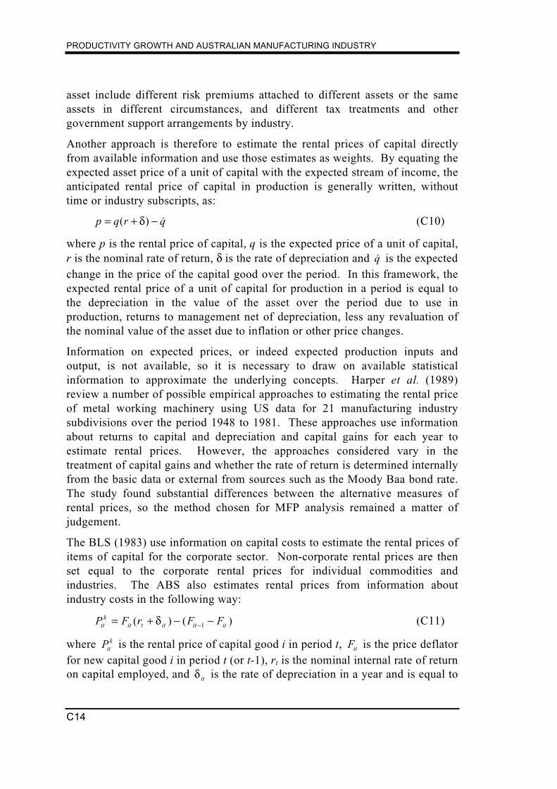
PRODUCTIVITY GROWTH AND AUSTRALIAN MANUFACTURING INDUSTRY
C14
asset include different risk premiums attached to different assets or the sameassets in different circumstances, and different tax treatments and othergovernment support arrangements by industry.
Another approach is therefore to estimate the rental prices of capital directlyfrom available information and use those estimates as weights. By equating theexpected asset price of a unit of capital with the expected stream of income, theanticipated rental price of capital in production is generally written, withouttime or industry subscripts, as:
p q r q= + −( )δ (C10)
where p is the rental price of capital, q is the expected price of a unit of capital,r is the nominal rate of return, δ is the rate of depreciation and q is the expectedchange in the price of the capital good over the period. In this framework, theexpected rental price of a unit of capital for production in a period is equal tothe depreciation in the value of the asset over the period due to use inproduction, returns to management net of depreciation, less any revaluation ofthe nominal value of the asset due to inflation or other price changes.
Information on expected prices, or indeed expected production inputs andoutput, is not available, so it is necessary to draw on available statisticalinformation to approximate the underlying concepts. Harper et al. (1989)review a number of possible empirical approaches to estimating the rental priceof metal working machinery using US data for 21 manufacturing industrysubdivisions over the period 1948 to 1981. These approaches use informationabout returns to capital and depreciation and capital gains for each year toestimate rental prices. However, the approaches considered vary in thetreatment of capital gains and whether the rate of return is determined internallyfrom the basic data or external from sources such as the Moody Baa bond rate.The study found substantial differences between the alternative measures ofrental prices, so the method chosen for MFP analysis remained a matter ofjudgement.
The BLS (1983) use information on capital costs to estimate the rental prices ofitems of capital for the corporate sector. Non-corporate rental prices are thenset equal to the corporate rental prices for individual commodities andindustries. The ABS also estimates rental prices from information aboutindustry costs in the following way:
P F r F Fitk
it t it it it= + − −−( ) ( )δ 1 (C11)
where Pitk is the rental price of capital good i in period t, Fit is the price deflator
for new capital good i in period t (or t-1), rt is the nominal internal rate of returnon capital employed, and δ it is the rate of depreciation in a year and is equal to

C LINKING MEASURES OF THE VALUE OF CAPITAL STOCKS AND CAPITAL CAPACITY
C15
the value of economic depreciation divided by the value of net capital stock atthe end of the year (Aspen 1990). The ABS computes the implicit nominalinternal rate of return on capital from information in capital income, the rate ofdepreciation and capital gains as:
rY
Vft
tk
tt
k= − −δ (C12)
where Ytk is the value of capital income estimated by the national accounting
aggregate gross operating surplus, Vtk is the value of net capital stocks at the
beginning of the year and f is the proportional growth in prices of capitalgoods. The ABS convention of including the implicit rate of return in the rentalprice calculations was found necessary because the rate of capital-good pricechange in any one year can be larger than a market (ie external) interest rateplus the rate of depreciation. Using this information and estimates of the levelof capital capacity, the single period factor share weights for each type ofcapital are then defined as:
sP K
P Kitk it
kit
itk
iti
=∑
(C13)
which is the capital-good component of the weighting pattern appropriate to themodel of MFP defined in equation D9 of Appendix D.
The OECD estimates total productive capital stocks used in its productivitystudies by adding capital stocks of machinery and equipment, and building andconstruction (OECD 1996). Estimates of the stocks of the two types of capitalgoods are estimated by the PIM as described above. Chand et al. (forthcoming)adopted a single category of capital and therefore aggregation was not an issuefor that study. Lattimore (1989) was concerned with the value of capital stocksrather than productive capacity. Appropriately, the separate estimates obtainedin that study for the value of plant and equipment, and buildings and structureswere directly aggregated using unit prices (and not rental prices) as weights.
Application of rental price weights to estimated changes in capitalcapacity levels
The level of capital capacity employed in an industry changes continuously inresponse to relative price changes, as does the mix between labour and capitalinputs. The adoption of fixed weighted indexes is often regarded as toorestrictive an assumption for the aggregation of changes in capital inputs forproductivity analysis. For example, when price and quantity relativities are
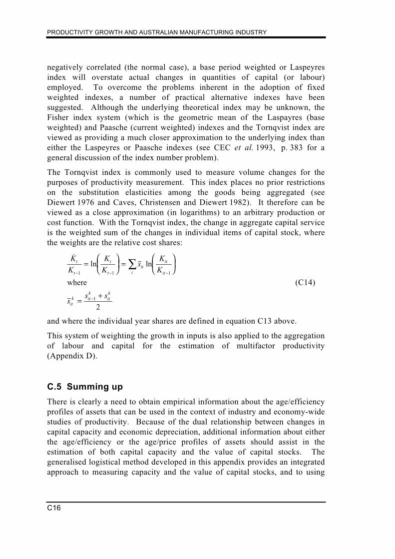
PRODUCTIVITY GROWTH AND AUSTRALIAN MANUFACTURING INDUSTRY
C16
negatively correlated (the normal case), a base period weighted or Laspeyresindex will overstate actual changes in quantities of capital (or labour)employed. To overcome the problems inherent in the adoption of fixedweighted indexes, a number of practical alternative indexes have beensuggested. Although the underlying theoretical index may be unknown, theFisher index system (which is the geometric mean of the Laspayres (baseweighted) and Paasche (current weighted) indexes and the Tornqvist index areviewed as providing a much closer approximation to the underlying index thaneither the Laspeyres or Paasche indexes (see CEC et al. 1993, p. 383 for ageneral discussion of the index number problem).
The Tornqvist index is commonly used to measure volume changes for thepurposes of productivity measurement. This index places no prior restrictionson the substitution elasticities among the goods being aggregated (seeDiewert 1976 and Caves, Christensen and Diewert 1982). It therefore can beviewed as a close approximation (in logarithms) to an arbitrary production orcost function. With the Tornqvist index, the change in aggregate capital serviceis the weighted sum of the changes in individual items of capital stock, wherethe weights are the relative cost shares:
ln lnK
K
K
Ks
K
K
ss s
t
t
t
tit
it
iti
itk it
kitk
− − −
−
=
=
=+
∑1 1 1
1
2
where (C14)
and where the individual year shares are defined in equation C13 above.
This system of weighting the growth in inputs is also applied to the aggregationof labour and capital for the estimation of multifactor productivity(Appendix D).
C.5 Summing up
There is clearly a need to obtain empirical information about the age/efficiencyprofiles of assets that can be used in the context of industry and economy-widestudies of productivity. Because of the dual relationship between changes incapital capacity and economic depreciation, additional information about eitherthe age/efficiency or the age/price profiles of assets should assist in theestimation of both capital capacity and the value of capital stocks. Thegeneralised logistical method developed in this appendix provides an integratedapproach to measuring capacity and the value of capital stocks, and to using

C LINKING MEASURES OF THE VALUE OF CAPITAL STOCKS AND CAPITAL CAPACITY
C17
additional information about either aspect of capital measurement to improveestimates of both.

PRODUCTIVITY GROWTH AND AUSTRALIAN MANUFACTURING INDUSTRY
C18

D1
APPENDIX DMULTIFACTOR PRODUCTIVITY GROWTH
ACCOUNTING
D.1 Growth accounting framework
The multifactor productivity growth accounting equation used throughout thisstudy is derived from the neoclassical theory of costs and production. Theappropriate shares for aggregating different categories of inputs and types ofcapital are derived from this basic theory which is set out below.
The neoclassical growth model is based on a production function with constantreturns to scale, capital and labour substitutability and diminishing marginalproductivities of inputs. The production function can be written:
( )Y Af K L= , (D1)
where Y is the measure of output in period t, K and L are effective inputs ofcapital and labour and A A t= ( ) is a shift term reflecting influences such aschanges in technology, the intensity with which labour and capital are used andorganisational improvements through time. Differentiating the productionfunction with respect to time gives:
dY
dtf
dA
dtA
f
K
dK
dtA
f
L
dL
dt= + ⋅ + ⋅∂
∂∂∂
(D2)
Thus, the change in output over time can be attributed to increases in the
deployment of effective inputs of labour and capital (iedK
dt
dL
dtand ), plus
organisational improvements that raise the level of production over time
(iedA
dt). If measures of the relative productivity of labour and capital
(ie∂∂
∂∂
f
K
f
Land ) were available, such measures could be used directly to obtain
a total measure of inputs. Similarly, various components of capital and labourcould be weighted together according to relative productivities.
However, measures of labour and capital productivity and multifactorproductivity growth are not directly observable, and it is necessary to useinformation about underlying production relationships to obtain measures that

PRODUCTIVITY GROWTH AND AUSTRALIAN MANUFACTURING INDUSTRY
D2
can be used in studies of growth. This is done in several steps. Dividing bothsides by Y, the level of output, to show changes per unit of output, noting thedefinition of Y in equation D1, and multiplying the capital and labour terms on
the right hand side by 1 = =K
K
L
L gives the expression:
dY
dt Y A
dA
dt
f
K
K
f K
dK
dt
f
L
L
f L
dL
dt
1 1 1 1= + +∂
∂∂∂
(D3)
By defining the proportional growth in output, capital and labour as y, k and l
and A A e aA
dA
dttt= = =0
1λ λwith (D3) can be written simply as:
y a k lk l= + +ε ε (D4)
where ε ∂∂
ε ∂∂k l
f
K
K
f
f
L
L
f= =and are the elasticities of output with respect to a
change in capital or labour inputs, respectively. Under the constant returns toscale assumption adopted in conventional growth accounting modelsε εk l+ = 1.
D.2 Aggregating factors of production using factor shares
Assuming competitive pricing of factor inputs, each factor would be paidaccording to its marginal product, in which case the elasticity of output forindividual factors is also the factor share in output. For capital inputs:
ε ∂∂k k
f
K
K
f
rK
fcapital shareof output s= = = = (D5)
where r is the real return per unit of capital inputs to production and s sk l+ = 1.The capital and labour shares in output can be readily obtained from basic datasources, providing a basis for aggregating inputs to production and obtainingestimates of multifactor productivity using equation D4. This formulation,however, is expressed in real terms while the capital share of output in basicdata sources is normally expressed in nominal terms. The application of thisapproach therefore also depends on the simplifying assumption that input andoutput prices move concurrently, which may not always be the case.
There is a somewhat more general assumption that can be made that enablesfactor input shares to be used as weights for the aggregation of inputs, at thesame time allowing relative prices between inputs to vary. The simple use offactor shares in MFP growth calculations defines MFP as:
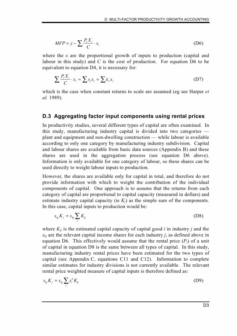
D MULTI-FACTOR PRODUCTIVITY GROWTH ACCOUNTING
D3
MFP yP X
Cxi i
i= − ⋅∑ (D6)
where the x are the proportional growth of inputs to production (capital andlabour in this study) and C is the cost of production. For equation D6 to beequivalent to equation D4, it is necessary for:
P X
Cx s x xi i
i i i i i∑ ∑ ∑⋅ ≈ = ε (D7)
which is the case when constant returns to scale are assumed (eg see Harper etal. 1989).
D.3 Aggregating factor input components using rental prices
In productivity studies, several different types of capital are often examined. Inthis study, manufacturing industry capital is divided into two categories ––plant and equipment and non-dwelling construction –– while labour is availableaccording to only one category by manufacturing industry subdivision. Capitaland labour shares are available from basic data sources (Appendix B) and theseshares are used in the aggregation process (see equation D6 above).Information is only available for one category of labour, so these shares can beused directly to weight labour inputs to production.
However, the shares are available only for capital in total, and therefore do notprovide information with which to weight the contribution of the individualcomponents of capital. One approach is to assume that the returns from eachcategory of capital are proportional to capital capacity (measured in dollars) andestimate industry capital capacity (ie Kj) as the simple sum of the components.In this case, capital inputs to production would be:
s K s Kkj j kj iji
= ∑ (D8)
where Kij is the estimated capital capacity of capital good i in industry j and theskj are the relevant capital income shares for each industry j, as defined above inequation D6. This effectively would assume that the rental price (Pi) of a unitof capital in equation D8 is the same between all types of capital. In this study,manufacturing industry rental prices have been estimated for the two types ofcapital (see Appendix C, equations C11 and C12). Information to completesimilar estimates for industry divisions is not currently available. The relevantrental price weighted measure of capital inputs is therefore defined as:
s K s s Kkj j kj ik
iji
= ∑ (D9)

PRODUCTIVITY GROWTH AND AUSTRALIAN MANUFACTURING INDUSTRY
D4
where sik is the rental price weight of each type of capital i (with separate
weights being calculated for each year t) (see equations C11 and C12 andsupporting discussion concerning rental price weighting of capital inputs).
D.4 Aggregating factor inputs using a generalised weightingsystem
Factors are aggregated at several levels in this study. First, items of capital areaggregated to form a composite capital good for each industry. Second, labourand capital inputs are aggregated using factor shares to provide a measure oftotal factor inputs into each industry. Finally, inputs are aggregated acrossindustries to form a market sector or manufacturing division total, asappropriate. Factor shares could be used directly in this process. However,those shares and the factor input measure to which they relate (ie hours workedfor labour and constant dollars for capital) refer to a single period (or a point intime in a single period in the case of capital). In order to provide moregeneralised indexes of inputs, it is common to form divisia indexes from theinformation available for successive periods. Broadly, such indexes useinformation from adjacent periods to form an average index that is not biased toproduction technologies adopted in either period. They are symmetric indexesthat are an average of the two situations being compared (ie successive years inproductivity analysis) and differ from fixed weighted indexes that weightchange according to the situation in either the first or the second period.
The Tornqvist index is commonly used to measure volume changes for thepurposes of productivity measurement.1 It is the measure used for aggregatinginputs by the BLS (1983) and ABS (see Aspen 1990). The Tornqvist volumeindex of factor inputs is defined as:
TX
Xxt
t
s
l
lt
=
−∏
1
(D10)
where ( )s s slt l t l t= +−1
2 1, , is the average relative factor share pertaining to the
respective inputs and Xt represents the relevant input (eg labour and capital) toproduction in year t, or t-1 as the case may be. The component shares are thefactor income or rental price shares, as defined above. Expressing the
1 Another generalised index which has similar properties to the Tornqvist is the Fisherideal index (see CEC et al. 1993, p. 379 and Diewert 1976).
D MULTI-FACTOR PRODUCTIVITY GROWTH ACCOUNTING
D5
proportional changes in logarithms, multifactor productivity growth of eachindustry can be expressed as:
a mfp y s k s l
yY
Yk
K
Kl
L
L
t t t tk
t tl
t
tt
tt
t
tt
t
t
≡ = − ⋅ − ⋅
=
=
=
− − −
where
andln , ln , ln1 1 1
(D11)
This formulation is applied in this study to estimate MFP growth by industrydivision in the market sector and manufacturing industry subdivision. From thedefinition of At above, the chain linked index of productivity levels over time isthen defined as:
A MFP MFP et t tmfpt≡ = −1 (D12)
where the reference period is the first year of the series, that is, 1974–75 forindustry divisions and 1968–69 for manufacturing subdivisions with A0=1. Thefinal estimates are obtained by re-referencing the series to 1989–90, thereference year for other series examined in this study.

PRODUCTIVITY GROWTH AND AUSTRALIAN MANUFACTURING INDUSTRY
D6

E1
APPENDIX ESENSITIVITY OF CAPITAL STOCK ESTIMATES
TO ALTERNATIVE ASSUMPTIONS
E.1 Introduction
As discussed in Chapter 5, there are many different approaches and conventionsthat can be used to estimate capital capacity and net capital stocks. Thisappendix reports the sensitivity of capital values to key data and methodologicalassumptions.
The first sensitivity analysis, outlined in section E.2, is a comparison ofalternative investment data. Section E.3 assesses the effect of differentmethodologies on capital capacity measures, while section E.4 examines theeffects of alternative asset depreciation methods and asset life assumptions.Section E.5 gives a comparison of Commission capital stocks with ABSestimates. A final section sums up the appendix.
In each of the sensitivity tests, the Commission’s generalised logistic, privatenet capital stock series, is used as the basis for comparison. Estimates for thecapital categories machinery and equipment and non-dwelling construction areconsidered in this appendix. However, as machinery and equipment dominatescapital expenditure (accounting for about 82 per cent of new capitalexpenditure), most sensitivity tests are reported for that capital item.
E.2 Alternative investment data
The quarterly survey of private new fixed capital expenditure currently providesthe most suitable basis for continuing productivity analysis at the disaggregatedmanufacturing level. In particular, it provides the industry detail required forthis study. The information is available over a long time period, and is updatedregularly from quarterly collections. Data by manufacturing subdivision overthe extended period are not available from any alternative source.
As discussed in Chapter 5, the new fixed capital series has a number ofdisadvantages when compared with the ABS measure of gross fixed capitalexpenditure for total manufacturing. On average, gross capital expenditure isapproximately 15 per cent higher than net capital expenditure, although the gap

PRODUCTIVITY GROWTH AND AUSTRALIAN MANUFACTURING INDUSTRY
E2
has narrowed over the period (Figure E.1). The main reasons for thisdiscrepancy are:
• the new capital expenditure series only records new investment and doesnot take into account the sales and purchases of second hand assets;
• the gross fixed capital expenditure series measures both private and publicinvestment, while new capital expenditure is a measure of only privateinvestment; and
• the ABS gross fixed capital expenditure data are derived from incometaxation statistics, while new capital expenditure data are based onenterprise surveys of the major activity undertaken by each industry.
Although the series differ in levels, the year to year changes are closely related.As a result, in change form, capital and productivity estimates are likely to beinsensitive to the investment series used.
Figure E.1: Comparison of investment measures, totalmanufacturing, 1968–69 to 1994–95 ($ million)
3500
5000
6500
8000
9500
1968
-69
1971
-72
1974
-75
1977
-78
1980
-81
1983
-84
1986
-87
1989
-90
1992
-93
Private new capital expenditureGross fixed capital expenditure
Sources: ABS special request and ABS catalogue 5221.0.
While the gap between the respective estimates for machinery and equipmenthas narrowed since the mid 1980s, the gap for non-dwelling construction, ifanything, has widened over the same period (Figure E.2).

E SENSITIVITY OF CAPITAL STOCK ESTIMATES TO ALTERNATIVE ASSUMPTIONS
E3
Figure E.2: Comparison of investment measures, non-dwellingconstruction and machinery and equipment, totalmanufacturing, 1968–69 to 1994–95 ($ million)
Non-dwelling construction Machinery and equipment
500
2000
3500
5000
6500
8000
1968
-69
1971
-72
1974
-75
1977
-78
1980
-81
1983
-84
1986
-87
1989
-90
1992
-93
New capital expenditure
Gross fixed capital expenditure
500
2000
3500
5000
6500
8000
1968
-69
1971
-72
1974
-75
1977
-78
1980
-81
1983
-84
1986
-87
1989
-90
1992
-93
New capital expenditure
Gross fixed capital expenditure
Sources: ABS special request and ABS catalogue 5221.0.
E.3 Capital capacity
To examine the sensitivity of capital capacity values to alternative assumptions,capital capacity series were estimated on four bases, the linear combination ofthe net and gross value capital stocks, geometric decline, hyperbolic decline andlogistic decline.
Figure E.3 and Table E.1 show that alternate methodologies have little impacton the annual change in the level of capital capacity. Nevertheless, thegeometric decay approach appears to differ more from the other methods thanthey do from one another. Under the geometric decay approach, asset capacityis assumed to decay more in the earlier years of service than under othermethods. This lowers the estimated level of installed capital capacity, resultingin greater year-to-year volatility than evident from other approaches. Inaddition, it results in annual capacity growth under this method generally lyingbelow growth implied by the other methods considered.
Results from the Commission’s logistic approach is also highly correlated withthe linear, geometric and hyperbolic approaches at the industry level. Thesensitivity of Commission estimates to alternative depreciation assumptions isdiscussed further in Section E.4.

PRODUCTIVITY GROWTH AND AUSTRALIAN MANUFACTURING INDUSTRY
E4
Figure E.3: Capital capacity based on alternative methodologies,total manufacturing, 1968–69 to 1994–95 ab (annualgrowth, per cent)
-3
0
3
6
9
1968
-69
1970
-71
1972
-73
1974
-75
1976
-77
1978
-79
1980
-81
1982
-83
1984
-85
1986
-87
1988
-89
1990
-91
1992
-93
1994
-95
Logistic Geometric Linear Hypobolic
a The linear and logistic efficiency decline approaches assume the assets have some residual value atretirement, whereas the geometric and hyperbolic approaches assume a zero residual value. With the exceptionof the logistic method introduced in this study, these conventions correspond to the common applications ofthese methods.Source: Commission estimates.
E.4 Value of capital stocks
The Commission uses capital capacity as its capital input measure for MFPstudies. Nevertheless, many studies of capital stocks are more concerned withthe value of capital rather than available capital capacity. These studies aregenerally presented within a national income and wealth framework. Value ofcapital series can be derived from capital capacity data or estimated directlyusing the PIM (Chapter 5). For sensitivity testing, capital value series havebeen derived for the logistic and hyperbolic asset age/efficiency profiles. Thesemeasures of capital stock can be compared with the measures obtained directlyusing the straight line and geometric decay methods. In addition, value ofcapital measures derived from the Commission’s logistic model have been usedto examine the sensitivity of model results to alternative compilationassumptions.

E SENSITIVITY OF CAPITAL STOCK ESTIMATES TO ALTERNATIVE ASSUMPTIONS
E5
Table E.1: Capital capacity based on alternative methodologies,manufacturing industry subdivision, 1968–69 to1994–95ab (average annual growth, per cent)
Industry Logistic Linear Geometric Hypobolic
Food, beverages and tobacco 3.419 3.333 0.961 2.191 0.872 3.505 0.979Textiles, clothing, footwear and leather 0.945 1.504 0.806 -0.090 0.872 1.258 0.697Printing, publishing and recorded media 4.750 4.301 0.946 3.769 0.949 5.479 0.936Petroleum, coal, chemical and associated products 1.488 1.835 0.896 0.392 0.864 1.643 0.974Basic metal products 3.017 3.116 0.970 1.697 0.949 3.070 0.988Fabricated metal products 2.128 2.410 0.963 0.867 0.955 2.285 0.995Transport equipment 3.036 3.140 0.930 1.489 0.888 3.202 0.983Other manufacturing 3.967 4.074 0.942 2.974 0.945 4.075 0.982
Total manufacturing 2.887 3.007 0.925 1.721 0.891 3.050 0.983
a The linear and logistic efficiency decline approaches assume the assets have some residual value atretirement, whereas the geometric and hyperbolic approaches assume a zero residual value. With the exceptionof the logistic method introduced in this study, these conventions correspond to the common applications ofthese methods.b Figures in italics represent the correlation coefficient between the logistic and the straight line, geometricdecay and hyperbolic series, respectively.Source: Commission estimates.
Although compilation assumptions are tested in a capital value framework, theconclusions should also apply to capital capacity measures, as appropriate.Although conceptually different, the conclusions should extend across bothframeworks as the value of capital series are derived from the capital capacityseries and the profiles of each are broadly similar (Appendix C).
Alternative depreciation methods
Depreciation, or the consumption of capital, is the reduction in the value ofcapital assets arising from use and obsolescence. The two main direct measuresof depreciation used in studies of the value of capital are the straight line (orlinear) and geometric decay (or diminishing balance) methods. In addition,both generalised logistic and hyperbolic methods for estimating capital capacityprovide implicit values for net capital stock and depreciation. This sectionexamines the sensitivity of capital value series to the alternative direct andimplicit estimation methods of depreciation (Figure E.4).

PRODUCTIVITY GROWTH AND AUSTRALIAN MANUFACTURING INDUSTRY
E6
Figure E.4: Net capital stocks based on alternative depreciationmethods, machinery and equipment, totalmanufacturing, 1968–69 to 1994–95 abc
Value of capital stocks ($ million) Annual growth (per cent)
10000
30000
50000
70000
1968
-69
1971
-72
1974
-75
1977
-78
1980
-81
1983
-84
1986
-87
1989
-90
1992
-93
Logistic Linear
Geometric
-3
0
3
6
9
1968
-69
1971
-72
1974
-75
1977
-78
1980
-81
1983
-84
1986
-87
1989
-90
1992
-93
Logistic Linear
Geometric
a Capital stocks at 30 June in each year.b Estimates assume Commission’s estimated asset lives and shortening of asset lives over time.c The logistic and hyperbolic series overlap almost entirely. The results for the hyperbolic series are notexplicitly shown.Source: Commission estimates.
Under the linear approach, assets are depreciated by equal amounts each yearand, as a result, the decline in an asset’s value is proportionately less in theearlier years of its life. The geometric, logistic and hyperbolic approachesadopt convex asset age/value profiles, although it is only under the geometricdecay method that the asset value declines in equal proportions in successiveyears. This means that, under these three approaches, asset values are assumedto fall faster than under the straight line method.
As a result, the straight line capital stock values for plant and equipment arelarger than the values estimated using alternative approaches — estimates of netcapital stock using the linear approach are about 20 per cent higher thanCommission estimates based on the logistic approach. However, in changeform, the hyperbolic, linear and geometric decay results are all highly correlatedwith the results from the Commission’s logistic approach, both in aggregate andat the industry subdivision levels of aggregation (Figure E.4 and Table E.2).

E SENSITIVITY OF CAPITAL STOCK ESTIMATES TO ALTERNATIVE ASSUMPTIONS
E7
Table E.2: Net capital stocks based on alternative depreciationmethods, machinery and equipment, by manufacturingindustry subdivision, 1968–69 to 1994–95 abc (averageannual growth, per cent)
Industry Logistic Linear Geometric Hypobolic
Food, beverages and tobacco 3.837 3.546 0.980 3.285 0.935 4.325 0.957Textiles, clothing, footwear and leather 1.644 1.081 0.952 1.149 0.965 1.839 0.988Printing, publishing and recorded media 7.101 5.070 0.927 5.495 0.971 8.152 0.919Petroleum, coal, chemical and associated products 1.295 1.176 0.977 1.037 0.973 1.384 0.981Basic metal products 2.566 2.310 0.994 1.959 0.979 3.204 0.980Fabricated metal products 2.035 2.241 0.992 1.777 0.985 2.187 0.995Transport equipment 4.589 4.312 0.983 4.152 0.983 4.845 0.977Other manufacturing 4.812 4.483 0.991 4.382 0.985 5.050 0.986
Total manufacturing 3.253 2.989 0.986 2.802 0.961 3.558 0.976
a Capital stocks at 30 June in each year.b Estimates assume Commission’s estimated asset lives and shortening of asset lives over time.c Figures in italics represent the correlation coefficient between the Commission’s estimates and the seriesundergoing the sensitivity test.Source: Commission estimates.
Alternative assumptions about asset lives
In this study, the asset life for each manufacturing industry is based on the ABSaverage with BIE industry relativities. In order to test the sensitivity of capitalstock estimates to alternative asset life assumptions, the value of capital stockshave also been estimated using the ABS 1980s average of 17 years for allindustries and the BIE estimates of asset lives for each industry subdivision.These alternative assumptions are examined using the Commission’s logisticmethodology.
The Commission’s estimates of the level of manufacturing industry net capitalstock are quite sensitive to asset life assumptions. Under BIE assumptions,capital is retired earlier than under either the Commission’s or the ABS’sassumptions, resulting in a lower level of net capital stocks (Figure E.5).
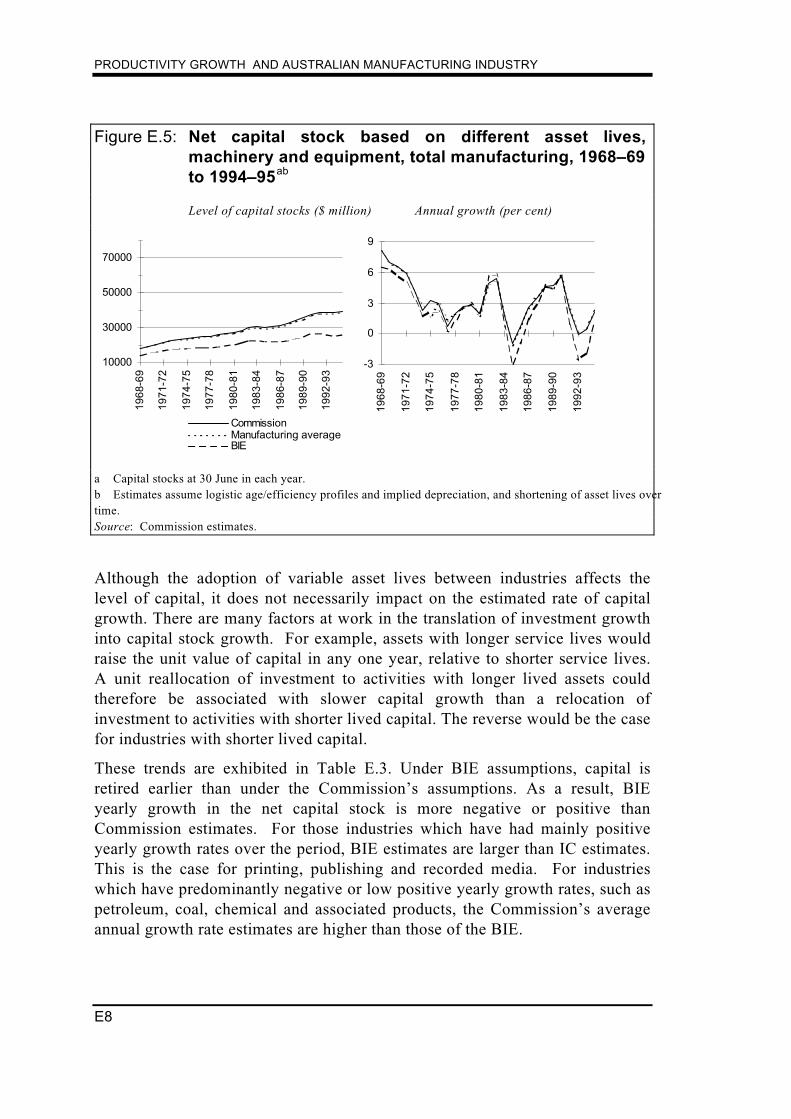
PRODUCTIVITY GROWTH AND AUSTRALIAN MANUFACTURING INDUSTRY
E8
Figure E.5: Net capital stock based on different asset lives,machinery and equipment, total manufacturing, 1968–69to 1994–95ab
Level of capital stocks ($ million) Annual growth (per cent)
10000
30000
50000
70000
1968
-69
1971
-72
1974
-75
1977
-78
1980
-81
1983
-84
1986
-87
1989
-90
1992
-93
CommissionManufacturing averageBIE
-3
0
3
6
9
1968
-69
1971
-72
1974
-75
1977
-78
1980
-81
1983
-84
1986
-87
1989
-90
1992
-93
a Capital stocks at 30 June in each year.b Estimates assume logistic age/efficiency profiles and implied depreciation, and shortening of asset lives overtime.Source: Commission estimates.
Although the adoption of variable asset lives between industries affects thelevel of capital, it does not necessarily impact on the estimated rate of capitalgrowth. There are many factors at work in the translation of investment growthinto capital stock growth. For example, assets with longer service lives wouldraise the unit value of capital in any one year, relative to shorter service lives.A unit reallocation of investment to activities with longer lived assets couldtherefore be associated with slower capital growth than a relocation ofinvestment to activities with shorter lived capital. The reverse would be the casefor industries with shorter lived capital.
These trends are exhibited in Table E.3. Under BIE assumptions, capital isretired earlier than under the Commission’s assumptions. As a result, BIEyearly growth in the net capital stock is more negative or positive thanCommission estimates. For those industries which have had mainly positiveyearly growth rates over the period, BIE estimates are larger than IC estimates.This is the case for printing, publishing and recorded media. For industrieswhich have predominantly negative or low positive yearly growth rates, such aspetroleum, coal, chemical and associated products, the Commission’s averageannual growth rate estimates are higher than those of the BIE.
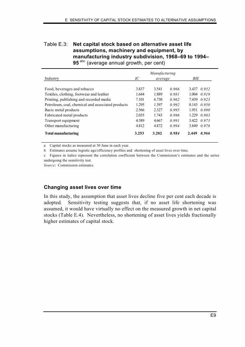
E SENSITIVITY OF CAPITAL STOCK ESTIMATES TO ALTERNATIVE ASSUMPTIONS
E9
Table E.3: Net capital stock based on alternative asset lifeassumptions, machinery and equipment, bymanufacturing industry subdivision, 1968–69 to 1994–95 abc (average annual growth, per cent)
Industry ICManufacturing
average BIE
Food, beverages and tobacco 3.837 3.541 0.966 3.437 0.952Textiles, clothing, footwear and leather 1.644 1.889 0.981 1.004 0.919Printing, publishing and recorded media 7.101 6.730 0.962 7.439 0.923Petroleum, coal, chemical and associated products 1.295 1.397 0.992 0.143 0.950Basic metal products 2.566 2.327 0.995 1.951 0.990Fabricated metal products 2.035 1.743 0.996 1.229 0.983Transport equipment 4.589 4.667 0.991 3.422 0.973Other manufacturing 4.812 4.872 0.994 3.849 0.978
Total manufacturing 3.253 3.202 0.984 2.449 0.966
a Capital stocks as measured at 30 June in each year.b Estimates assume logistic age/efficiency profiles and shortening of asset lives over time.c Figures in italics represent the correlation coefficient between the Commission’s estimates and the seriesundergoing the sensitivity test.Source: Commission estimates.
Changing asset lives over time
In this study, the assumption that asset lives decline five per cent each decade isadopted. Sensitivity testing suggests that, if no asset life shortening wasassumed, it would have virtually no effect on the measured growth in net capitalstocks (Table E.4). Nevertheless, no shortening of asset lives yields fractionallyhigher estimates of capital stock.

PRODUCTIVITY GROWTH AND AUSTRALIAN MANUFACTURING INDUSTRY
E10
Table E.4: Net capital stock based on alternative assumptions ofasset life shortening, machinery and equipment, bymanufacturing industry subdivision, 1968–69 to 1994–95abc (average annual growth, per cent)
Industry Asset shortening No asset shortening
Food, beverages and tobacco 3.837 4.129 0.999Textiles, clothing, footwear and leather 1.644 2.216 0.998Printing, publishing and recorded media 7.101 7.484 0.999Petroleum, coal, chemical and associated products 1.295 1.829 0.998Basic metal products 2.566 3.107 1.000Fabricated metal products 2.035 2.561 0.999Transport equipment 4.589 5.108 0.999Other manufacturing 4.812 5.285 0.999
Total manufacturing 3.253 3.711 0.999
a Capital stocks at 30 June in each year.b Estimates assume logistic age/efficiency profiles and the Commission’s estimated asset lives.c Figures in italics represent the correlation coefficient between the Commission’s estimates and the serieswhere assets lives have not been shortened over time.Source: Commission estimates.
Comparison of value of capital stocks with ABS estimates
The Commission’s approach to compiling capital stock estimates differs fromthat of the ABS in terms of methodology and investment data used. The ABScalculates capital stock estimates for manufacturing using gross fixed capitalexpenditure, while the Commission is constrained to using new capitalexpenditure to calculate capital stocks at the disaggregated manufacturingsubdivision level. Both studies assume that asset lives decline five per centeach decade. However, the ABS assumes straight line depreciation and uniformasset life across all industries (reference 17 years in the 1980s), while theCommission applies a generalised logistic model with asset lives based on theABS average with BIE industry subdivision relativities.
Prior sensitivity tests found that gross fixed capital expenditure and straight linedepreciation produced higher measured net capital stocks than those producedusing new capital expenditure and depreciation implicit in logisticage/efficiency profiles. As a result, the ABS level of capital stocks is higherthan Commission estimates. However, in growth form, the two series followsimilar paths (Figures E.6 and E.7 ).

E SENSITIVITY OF CAPITAL STOCK ESTIMATES TO ALTERNATIVE ASSUMPTIONS
E11
Figure E.6: ABS and Commission estimates of net capital stocks,machinery and equipment, total manufacturing, 1968–69to 1994–95ab
Value of capital stocks ($ million) Annual growth (per cent)
10000
30000
50000
70000
1968
-69
1972
-73
1976
-77
1980
-81
1984
-85
1988
-89
1992
-93
ABS Commission
-3
0
3
6
9
1968
-69
1971
-72
1974
-75
1977
-78
1980
-81
1983
-84
1986
-87
1989
-90
1992
-93
ABS Commission
a Capital stocks as measured at 30 June in each year.b The ABS assumes straight line depreciation and uniform asset lives across all manufacturing industries.The Commission assumes logistic age/efficiency profiles and different asset lives between manufacturingindustry subdivisions. Both series assume that asset lives are shortened by 5 per cent each decade.Sources: ABS 1997c, Commission estimates.
Figure E.7: ABS and Commission estimates of net capital stocks,total manufacturing, 1968–69 to 1994–95 ab
Value of capital stocks ($ million) Annual growth (per cent)
10000
30000
50000
70000
1968
-69
1972
-73
1976
-77
1980
-81
1984
-85
1988
-89
1992
-93
ABS Commission
-3
0
3
6
9
1968
-69
1972
-73
1976
-77
1980
-81
1984
-85
1988
-89
1992
-93
ABS Commission
a Capital stocks as measured at 30 June in each year.b The ABS assumes straight line depreciation and uniform asset lives across all industries and that asset livesare shortened by 5 per cent each decade. The Commission assumes logistic depreciation, different asset livesbetween manufacturing industries and that asset lives are shortened by 5 per cent each decade.Sources: ABS 1997c, Commission estimates.

PRODUCTIVITY GROWTH AND AUSTRALIAN MANUFACTURING INDUSTRY
E12
E.5 Summing up
While different investment data, alternative depreciation methods and varyingasset lives can have a substantial effect on the estimated level of capital, theyhave only a limited impact on year-to-year changes in estimates of capitalcapacity and the value of net capital stock.
In terms of the individual sensitivity tests conducted, the Commission’sestimated value of net capital stock obtained from its generalised logisticmethod differs most from estimates based on linear depreciation. Estimatedlevels are also sensitive to alternative assumptions about asset lives. However,alternative depreciation and asset life assumptions have little effect on theaverage annual growth in the value of net capital stocks, which are primarilydriven by changes in investment.
As alternative investment series follow similar trends, the Commission’s finalestimates of annual growth in capital capacity and the value of net capital stockcompare closely with estimates based on alternative data sources.

References 1
REFERENCES
ABS 1973, Australian Standard Industrial Classification (ASIC) 1969 Edition,Cat. No. 1201.0, mimeo, Canberra.
—— 1979, Australian Standard Industrial Classification (ASIC) 1978 Edition,Cat. No. 1201.0, mimeo, Canberra.
—— 1985, Australian Standard Industrial Classification (ASIC) 1983 Edition,Cat. No. 1201.0, mimeo, Canberra.
—— 1989, (and previous years), Enterprise Statistics Australia, Cat.No. 8103.0, mimeo, Canberra.
—— 1990, Australian National Accounts,Concepts, Sources and Methods, Cat.No. 5216.0, AGPS, Canberra.1
—— 1993, Australian and New Zealand Standard Industrial Classification(ANZSIC) 1993 Edition, Cat. No. 1292.0, AGPS, Canberra.
—— 1996a, Private New Capital Expenditure and Expected Expenditure toJune 1997, Australia, Cat. No. 5625.0, mimeo, Canberra.
—— 1996b (and previous years), Manufacturing Industry, Australia 1994–95,Cat. No. 8221.0, mimeo, Canberra.
—— 1997a, (and previous years), Australian National Accounts: NationalIncome, Expenditure and Product 1995–96, Cat. No. 5204.0, AGPS, Canberra.
—— 1997b (and previous years), Australian National Accounts: Input-OutputTables 1993–94, Cat. No. 5209.0, AGPS, Canberra.
—— 1997c (and previous years), Australian National Accounts: Capital Stock,Cat. No. 5221.0, AGPS, Canberra.
—— 1997d, (and previous years), Australian National Accounts: MultifactorProductivity 1995–96, Cat. No. 5234.0, mimeo, Canberra.
—— 1997e (and previous years), Australian National Accounts: NationalBalance Sheets, Cat. No. 5241.0, AGPS, Canberra.
—— 1997f (and previous years), Labour Force, Australia, Cat. No. 6203.0,mimeo, Canberra.
1 Concepts, sources and methods to the national accounts are also available in ABS 1996,Statistical Concepts Reference Library, on CD-ROM, Cat. No. 1361.0, AGPS,Canberra.

PRODUCTIVITY GROWTH AND AUSTRALIAN MANUFACTURING INDUSTRY
References 2
—— 1997g, Monthly Labour Force Survey (unpublished data), Canberra.
Aspen C. 1990, Estimates of Multi-factor Productivity, Australia, ABSOccasional Paper, Cat. No. 5233.0, mimeo, Canberra.
Bailey, C. 1981, Current-Cost and Constant-Cost Depreciation and Net CapitalStocks, Studies in National Accounting 1981/1, mimeo, Canberra.
Boskin, M.J., Robinson, M.S. and Huber, A.M. 1989, ‘Government Saving,Capital Formation and Wealth’, ed. Robert E. Lipsey and Helen Stone Tice, TheMeasurement of Savings Investment and Wealth, NBER Studies in Income andWealth, Vol. 52, University of Chicago Press, Chicago, pp 287–353.
Boskin, M.J., Robinson, M.S. and Roberts, J.M. 1989, ‘New Estimates ofFederal Government Tangible Capital and Net Investment’, ed. D.W. Jorgensonand R. Landau, Technology and Capital Formation, MIT Press, Cambridge,pp 451–483.
Bureau of Industry Economics (BIE) 1985, Productivity Growth in AustralianManufacturing Industry, Information Bulletin No. 8, AGPS, Canberra.
Caves, D.W., Christensen, L.R., and Diewert, W.E. 1982, ‘The Theory of IndexNumbers and the Measurement of Input, Output and Productivity’,Econometrica, Vol. 50, No. 6, pp 1393–1414.
Chand, S., Forsyth, P., Sang, M. and Vousden, N. (forthcoming), Total FactorProductivity, a 14 Country Study, mimeo, ANU, Canberra.
Chand, S. and Vousden, N. (forthcoming), Trade Liberalization andProductivity Growth: A Panel Data Study of Australian Manufacturing,Australian National University, Canberra.
Chand, S. 1997, Trade Liberalisation and Productivity Growth: Time seriesEvidence from Australian Manufacturing, Australian National University,Canberra.
Commission of European Communities, International Monetary Fund,Organisation for Economic Cooperation and Development, United Nations,World Bank (CEC et al.) 1993, System of National Accounts, 1993, CEC et al.,Brussels/Luxemberg, New York, Paris, Washington.
Diewert, W.E. 1976, ‘Exact and Superlative Index Numbers’, Journal ofEconometrics, Vol. 4, No. 4, pp 115–145.
EconData 1997, dX for Windows: the time series data express, Version 2.0,EconData, Canberra, data at July 1997.

REFERENCES
References 3
Fraumeni, B.M., and Jorgenson, D.W. 1986, ‘The Role of Capital in USEconomic Growth, 1948–1979’, in Ali Dogramaci, Measurement Issues andBehavior of Productivity, Martinus Nijhoff, Boston.
Glass’s Guide 1997, Passenger Vehicles, February 1997 Edition, Melbourne.
Haig, B. 1980, Capital Stocks in Australian Manufacturing, Department ofEconomics, Research School of Social Sciences, Australian NationalUniversity, Canberra.
Harper M.J., Berndt E.R. and Wood D.O. 1989, ‘Rates of Return and CapitalAggregation Using Alternative Rental Prices’ ed. Jorgenson D.W. and LandauR., Technology and Capital Formation, MIT Press, Cambridge, pp 331–372.
Hourigan, 1980, Estimation of an Australian Capital Stock Matrix for theIMPACT Project, Working Paper No. I-11, Impact Project, Melbourne.
Hulten C. 1990, ‘The Measurement of Capital’, in Berndt E. and Triplett J.,Fifty Years of Economic Measurement: The Jubilee of the Conference onResearch in Income and Wealth, University of Chicago Press, Chicago.
Hulten, C.R. and Wykoff, F.C. 1981, ‘The Estimation of EconomicDepreciation Using Vintage Asset Prices: an application of the Box-Cox PowerTransformation’, Journal of Econometrics, 15 (1981), pp 367—396.
Industry Commission (IC) 1995a, Research and Development, Report No. 44,AGPS, Canberra.
–– 1995b, Assistance to Agriculture and Manufacturing Industries, InformationPaper, AGPS, Canberra.
–– 1995c, Australian Manufacturing Industry and International Trade Data,1968–69 to 1992–93, AGPS, Canberra.
–– 1997, Assessing Australia’s Productivity Performance, Information Paper,AGPS, Canberra.
Jorgensen, D.W., Gallop, F.M. and Fraumeni, B.M. 1987, Productivity and USEconomic Growth, Harvard University Press, Boston.
Karpouzis, G. and Offner, T. 1983, Capital Stocks of Plant and Equipment inthe Australian Manufacturing Sector, Bureau of Industry Economics WorkingPaper No. 28, Bureau of Industry Economics, Canberra.
Kenderes, M. and Strzelecki, A. 1991, Listing of the 1986–87 ORANI DataBase, Research Memorandum ORANI No. OA–569, Industry Commission,Canberra, revised February 1992.

PRODUCTIVITY GROWTH AND AUSTRALIAN MANUFACTURING INDUSTRY
References 4
Lattimore, R. 1989, Capital Formation in Australian Manufacturing, 1954-55to 1987-88, BIE Working Paper No. 54, mimeo, Canberra.
Leamer, E. 1988, ‘The sensitivety of international comparisons of capital stockmeasures to different real exchange rates’, American Economic Review: Papersand Proceedings, No. 78, pp 479–483.
Meyer zu Schlochtern, F.J.M. and Meyer zu Schlochtern, J.L. 1994, AnInternational Sectoral Data Base for Fourteen OECD Countries (SecondEdition), Economics Department Working Papers No. 145, OECD, Paris.
Organisation for Economic Cooperation and Development (OECD) 1993,Methods Used by OECD Countries to Measure Fixed Capital, NationalAccounts: Sources and Methods No.2, OECD, Paris.
—— 1996, International Sectoral Data Base ISDB 96, Statistics Directorate,OECD, Paris.
Pearce, D.W. and Turner, R.K. 1990, Economics of Natural Resources and theEnvironment, Harvester Wheatsheaf, New York.
Reserve Bank of Australia (RBA) 1996a, Estimation of Capital Stock for EightManufacturing Sub-Divisions since June 1959, unpublished working paper,Sydney.
-- (1996b), Australian Economic Statistics 1949–50 to 1994–95, Reserve Bankof Australia Occasional Paper No. 8, Sydney.
Solow, R.M. 1956, ‘A Contribution to the Theory of Economic Growth’,Quarterly Journal of Economics, No. 70, pp 65–94.
Swan, T.W. 1956, ‘Economic Growth and Capital Accumulation’, EconomicRecord, No. 32, pp 332–361.
Triplett, J.E. 1996, ‘Depreciation in Production Analysis, and Income andWealth Accounts: Resolution of an Old Debate’, Economic Inquiry, Vol.XXXIV, January 1996, pp 93–115.
US Department of Labour, Bureau of Labour Statistics (BLS) 1983, Trends inMulti-factor Productivity, 1948–81, Bulletin No. 2178, Government PrintingOffice, Washington D.C.
Walters, R. and Dippelsman, R. 1985, Estimates of Depreciation and CapitalStock Australia, Australian Bureau of Statistics Occasional Paper No. 1985/3,ABS, Canberra.

REFERENCES
References 5