productivity measurement and analysis: techniques … measurement and... · productivity...
TRANSCRIPT

Productivity Measurement and Analysis: Techniques and
Applications
Bishwanath Goldar
Institute of Economic Growth, Delhi
November 2015

Outline of Presentation Introduction: insights gained from productivity
analysis, two examples Alternate approaches to productivity measurement Conceptual framework Alternate Methodology and applications
Total factor productivity (TFP) Indices (Tornqvist) Multilateral TFP Index Data Envelopment Analysis (DEA) – technical efficiency Malmquist Index – technical change and technical efficiency
change Levinsohn-Petrin Methodology – TFP estimates Stochastic frontier production function (not discussed).

Insights gained from productivity analysis, two examples relating to labour
0
1
2
3
4
5
6
7
8
9
1980-1990 1990-2000 2000-2007
perc
ent
per
ann
um
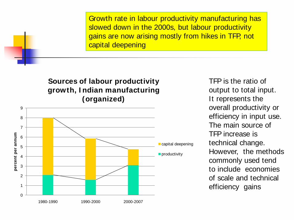
Sources of labour productivity growth, Indian manufacturing
(organized)
capital deepening
productivity
Growth rate in labour productivity manufacturing has slowed down in the 2000s, but labour productivity gains are now arising mostly from hikes in TFP, not capital deepening
TFP is the ratio of output to total input. It represents the overall productivity or efficiency in input use. The main source of TFP increase is technical change. However, the methods commonly used tend to include economies of scale and technical efficiency gains
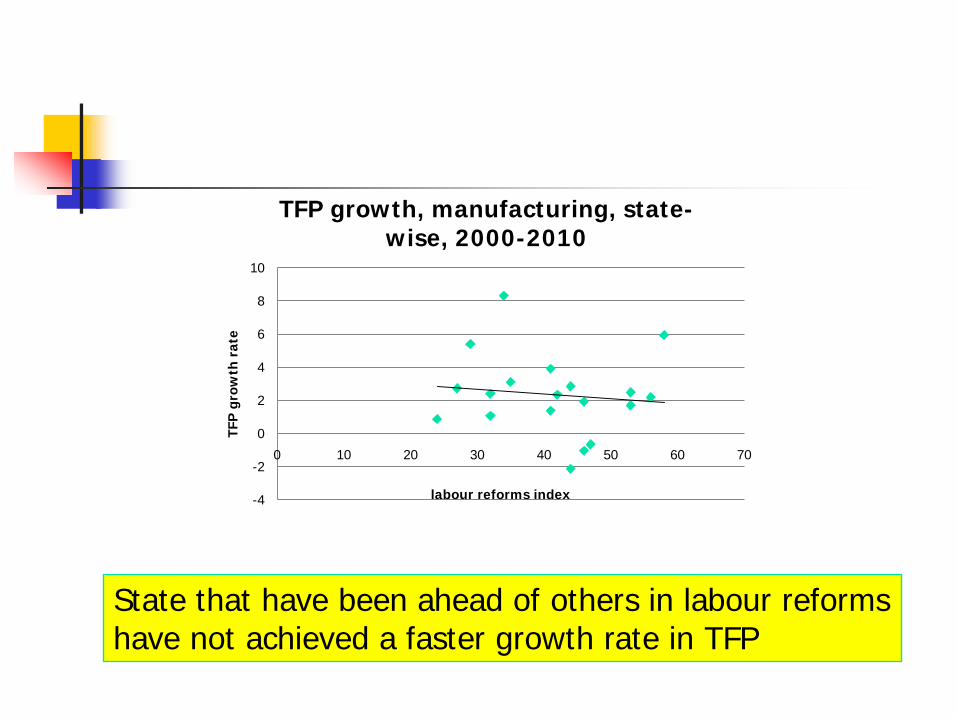
State that have been ahead of others in labour reforms have not achieved a faster growth rate in TFP
-4
-2
0
2
4
6
8
10
0 10 20 30 40 50 60 70
TFP
gro
wth
rat
e
labour reforms index
TFP growth, manufacturing, state-wise, 2000-2010

-4
-2
0
2
4
6
8
10
TFP growth rate, manufacturing, state-wise, 2000-2010
inflexibleflexible
States with inflexible labour market has not performed relatively worse in terms of TFP growth

Alternate approaches

Approaches to productivity measurement and analysis
Grwoth accountancyDivisia index
Tornquivist index
non-parametric
Econometric approaches,estimation of production function
parametric
Non-Frontier approach
Malmquist index
non-Parametric
Stochastic and deterministicfrontier function, estimated
econmertrically or LP
parametric
Frontier approach
productivity measurement

Which technique to use?Method
Translog TFP Index Multilateral TFP Index Malmquist Index Levinsohn-Petrin
methodology (or other methodology of same type)
Data envelopment analysis
Stochastic frontier production function
Type of data with the researcher (examples) Annual time series for
one industry for 10 years Annual time series for 10
industries for15 years

Which technique to use?Method
Translog TFP Index Multilateral TFP Index Malmquist Index Levinsohn-Petrin
methodology (or other methodology of same type)
Data envelopment analysis
Stochastic frontier production function
Type of data with the researcher Cross section data for one
industry for 25 states, one year
Panel data for one industry covering 25 states for 10 years

Which technique to use?Method
Translog TFP Index Multilateral TFP Index Malmquist Index Levinsohn-Petrin
methodology (or other methodology of same type)
Data envelopment analysis
Stochastic frontier production function
Type of data with the researcher Panel data for for 3000
factories belonging to one industry for 10 years
Cross section data on 30 factories belonging to one industry for one year
Cross section data for 3000 factories belonging to one industry for one year

Productivity level versus productivity growth Some methods give the growth rate in
productivity, some give the level of productivity.
Some methods give both the level and growth rate in productivity.

Conceptual framework

Relation between LP and KI
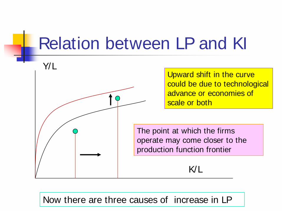
K/L
Y/L
As capital intensity increases over time, labour productivity goes up. LP increase due to capital deepening

Relation between LP and KI
K/L
Y/LUpward shift in the curve could be due to technological advance or economies of scale or both. LP increase is party due to capital deepening, partly due to TFP increase.
Relation between LP and KI
K/L
Y/LUpward shift in the curve could be due to technological advance or economies of scale or both
The point at which the firms operate may come closer to the production function frontier
Now there are three causes of increase in LP

Sources of gain in labour productivity
Increase in LP
Increase in capital intensity: factor substitution
Increase in the level of production: economies of scale
Technical change, new knowledge
Increase in technical efficiency: say, better utilization of capacity, greater motivation of labour

Productivity and efficiency Changes in productivity occur due to
changes in technology and changes in efficiency (how well the technology is used). Thus, the rate of productivity growth is the sum of the rate of technical progress and the rate of improvement in technical efficiency.

Technical (in)efficiency
X
X
XX
X
X
X
labour
Capital
O
Unit isoquant; combinations of labour and capital that can produce one unit of output
This firm is inefficient; the extent of inefficiency is indicated by the distance from the isoquant
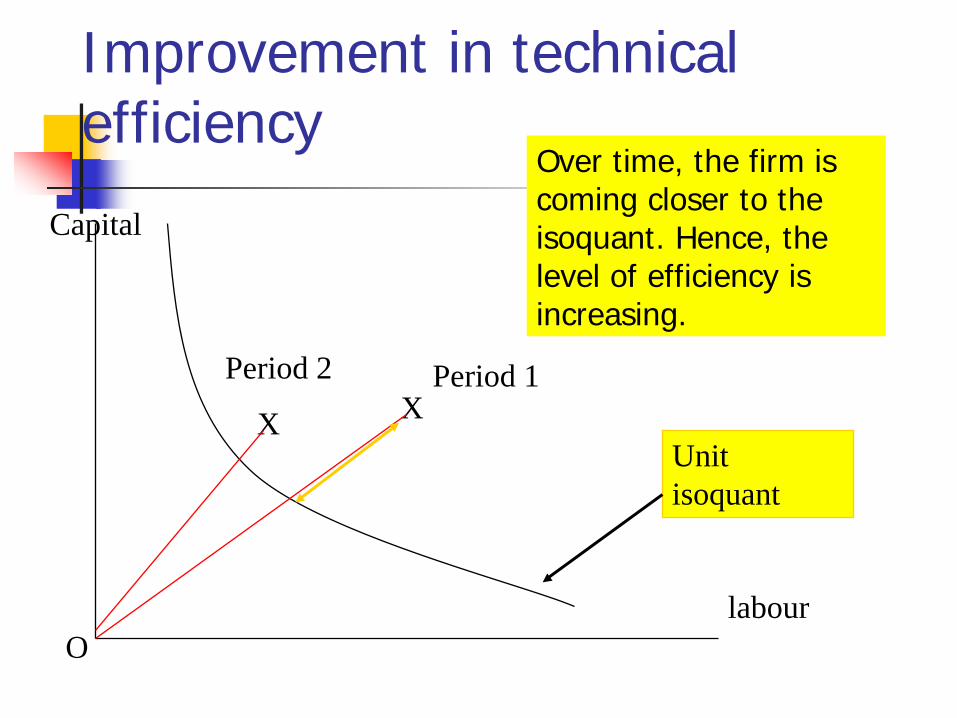
Improvement in technical efficiency
X X
labour
Capital
O
Unit isoquant
Period 1Period 2
Over time, the firm is coming closer to the isoquant. Hence, the level of efficiency is increasing.

Technical change (progress)
labour
capital
Unit isoquant period 1
Unit isoquant period 2
Rate of technical progress is given by the rate of inward shift of isoquant
XX*
Tornqvist index assumes that the firms are always on the isoquant

L
K
XX*
K=capital; L=labor
X and X* input use per unit of output in period 0 and 1
Unit isoquant, period=0
Unit isoquant, period=1
Shift in production function; technical change
Decline in technical inefficiency
Q: How do we split, the movement from X to X* into the three parts?
Factor substi-tution

Total factor Productivity –Divisia Index, Tornqvist index (Growth accounting)

Measurement of Total Factor Productivity -Growth accounting
Growth accounting: In this approach, TFP indices are used for measuring TFP.
TFP is defined as Y/I, where Y is the index of output, and I is the index of total input.
The income shares of the factors of production are used as weights to compute the growth in total input.
Similarly, when there are several output, revenue shares are used to combine growth of different outputs to form the growth rate in total output.

One output, three-input case (gross output function framework)

Growth accounting equation Y=f(L, K, X; t) : production function Taking total derivative
Dividing by Y
Y = output (real); L = labor input; K = capital input; X = intermediate input; t=time
tY
dtdX
XY
dtdK
KY
dtdL
LY
dtdY
∂∂
+∂∂
+∂∂
+∂∂
=
YtY
YdtdX
XY
YdtdK
KY
YdtdL
LY
YdtdY 11111
∂∂
+∂∂
+∂∂
+∂∂
=

Growth accounting equation(2)
One can derive
Y = output (real); L = labor input; K = capital input; X= intermediate inputs; SL = income share of labor; SX= income share of int. input, and SK = inc. share of capital (= 1-SL-SX)
YtY
XX
YdtdX
XY
KK
YdtdK
KY
LL
YdtdL
LY
YdtdY 11111
∂∂
+∂∂
+∂∂
+∂∂
=
tY
YX
dtXd
XY
YK
dtKd
KY
YL
dtLd
LY
dtYd
∂∂
+∂∂
+∂∂
+∂∂
=lnlnlnlnln
tY
dtXdS
dtKdS
dtLdS
dtYd
XKL ∂∂
+++=lnlnlnlnln
TFP growth

Tornqvist index/ Translog index of TFP
)](ln2
)1()([
)](ln2
)1()([)](ln2
)1()([)(ln)(ln
tXtSXtSX
tKtSKtSKtLtSLtSLtYtTFP
∆×−+
−
∆×−+
−∆×−+
−∆=∆
TFP = total factor productivity; Y = output (real)L = labor input; K = capital input; X= intermediate input; SL = income share of labor, SX= income share of int. input; and SK = share of capital (= 1-SL-SX)
The Translog index of TFP is commonly used for measuring TFP growth. It does not require the assumption of neutral technical change and allows for variable elasticity of substitution. It may be written as:

Translog index of TFP
TFP = total factor productivity; Y = value added (real)
L = labor input; K = capital input; SL = income share of labor, SX= inc. share of int. input, SK = share of capital (= 1-SL-SX)
Average income share of two years is taken
Growth rates in output, intermediate input, labor and capital
)](ln2
)1()([
)](ln2
)1()([)](ln2
)1()([)(ln)(ln
tXtSXtSX
tKtSKtSKtLtSLtSLtYtTFP
∆×−+
−
∆×−+
−∆×−+
−∆=∆
Compute in Excel

Translog/Tornqvist index -assumptions Constant returns to scale Competitive equilibrium – producers
maximize profits – minimize cost – input combination is so chosen that marginal product of each factor is equal to its price
Disembodied technical change – firms can take advantage of new technology without changing input use

One output, two-input case (value added function framework)

Growth accounting equation Y=f(L, K; t) : production function Taking total derivative
Y = value added (real); L = labor input; K = capital input; t=time
tY
dtdK
KY
dtdL
LY
dtdY
∂∂
+∂∂
+∂∂
=

Tornqvist index/ Translog index of TFP
)](ln2
)1()([)](ln2
)1()([)(ln)(ln tKtSKtSKtLtSLtSLtYtTFP ∆×−+
−∆×−+
−∆=∆
TFP = total factor productivity; Y = value added (real)L = labor input; K = capital input; SL = income share of labor; and SK = share of capital (= 1-SL)
Compute in Excel

Translog index of TFP - What is the problem, and how is that solved?
K/L
Y/L
A
B
Period 1
Period 2
C
A to C is factor substitution; C to B is technical change, or TFP growthSince we do not have the production function (i.e. the curves), we do not know where to fix point C

One way out
K/L
Y/L
A
BPeriod 1
Period 2
CA to C is factor substitution; C to B is technical change, or TFP growth
C’
Use the slope at point A to approximate. Slope= income share of capital in output (under perfect competition)

Better approximation
K/L
Y/L
A
BPeriod 1
Period 2
C A to C is factor substitution; C to B is technical change, or TFP growth
C’
Take average of slopes at points A and B to approximate. Slope= income share of capital in output. This brings C’ closer to true C. This is what Tornqvist index does.

ApplicationNIC Description TFP growth rate
1999 to 2011 (% p.a.)
15 Food products and beverages 1.15
16 Tobacco products -2.87
30+32+33 Electronics, computers, mobiles
12.19
34 Motor vehicles 2.53
All manufacturing 1.70
B. Goldar, Productivity in Indian Manufacturing (1999-2011): accounting for imported materials input, EPW, August 29, 2015. Five inputs considered: capital, labour, energy, materials, services (KLEMS).
Multilateral total factor productivity index

Labour productivity, level and growth, Org mfg by state
0
20
40
60
80
100
120
140
160
LP index (2003), Mah=100
LP grrowth rate (2003-2008), % per annum

Multilateral total factor productivity index
If one wants to study variations in TFP across regions (or firms) and over time, then a multilateral TFP index can be used.
If there are only two inputs, labour and capital, the multilateral TFP index may be written as:

Multilateral TFP Index
cCbb
KLKL cc
bbc
bbc
KLKLY
YTFP
βαβα
= __
__
The index expresses the productivity level in region-year b (say, UP in 2004) as a ratio to the productivity level in region-year c (say, Punjab in 2000). L and K with bar are sample average (geometric mean). The coefficients represent incomes shares of labour and capital.
Compute in Excel

Weights in the index Let SLb be the income share of labour in
state-year b and SL the arithmetic mean of labour share in value added across all the observations. Then, αb may be written as:
αc, βb and βc may be defined in a similar way.
2LSSLb
b+
=α

What Multilateral TFP Index compares?
State 1 State 2 State 3 State 4
Year 1 c b
Year 2 b
Year 3 b
Year 4 b

Assumptions Underlying the Index Constant returns to scale Factors paid according to marginal
product
References Basic methodology: D. Caves, L. R. Christensen,
and D. E. Diewert, “Multilateral comparisons of output, input and productivity using superlative index numbers.” Economic Journal, 92: 73-86, 1982.
Application to Indian industry, state-wise comparison: C. Veeramani and B. Goldar, “Manufacturing Productivity in Indian States: Does Investment Climate Matter?” Economic and Political Weekly, June 11, 2005.

Andhra Pradesh 0.60 0.77Gujarat 0.71 0.96Haryana 0.77 1.14Karnataka 0.64 0.94Maharashtra 1.00 1.17Orissa 0.57 0.72Tamil Nadu 0.70 0.79Uttar Pradesh 0.57 0.89West Bengal 0.76 0.72
Multi-lateral TFP index (MAH, 1998=1.00)
1998-99 2003-04

INVESTMENT CLIMATE & TFP (VALUE ADDED FUNCTION)
MAH
DEL
GUJ
AP
KAR PUNTN
HAR
MPKER
WB
UP
R2 = 0.543
50
70
90
110
130
150
0 1 2 3 4 5 6 7 8 9 10 11 12 13
Ranking of states according to IC
TFP
AV (1
992-
93 to
199
9-00
)
Regression line is fitted and R2 is computed without including Andhra Pradesh. C. Veeramani and B. Goldar, 2005, EPW

Technical Efficiency, Concept and measurement
Efficiency Efficiency (or technical efficiency to be
more specific) may be defined as the ratio of actual output to the potential/optimal output from a given bundle of inputs and given technology.
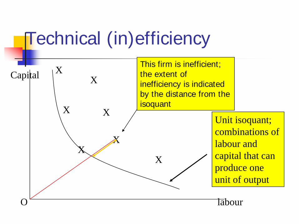
Technical (in)efficiency
X
X
XX
X
X
X
labour
Capital
O
Unit isoquant; combinations of labour and capital that can produce one unit of output
This firm is inefficient; the extent of inefficiency is indicated by the distance from the isoquant

Data Envelopment Analysis (DEA)

DEA
Data envelopment analysis (DEA) is widely used for studying technical efficiency in cross-sectional context.

DEA Main advantage of DEA: it does not impose
any functional form on the production function. Based on the observed input-output points, the best practice production frontier is derived and firms/regions are compared to the best practice frontier.
Another advantage is that this methodology does not need data on input (or output) prices.
The disadvantage is that the results are sensitive to outliers.

Technical (in)efficiency
X
X
XX
X
X
X
labour
Capital
O
Unit isoquant
We can find the level of inefficiency, if the isoquant is known. But, if it is not known, how can we estimate technical efficiency? DEA provides a solution (see next slide).

Technical (in)efficiency
X
X
XX
X
X
X
labour
Capital
O
DEA frontier, taken to represent Unit isoquant
Software, priced and free, are available to estimate DEA frontier and technical efficiency
Use DEAP 2.1 of Tim Coelli, freely downloadable for calculating TE

An empirical analysis of district hospitals and grant-in-aid hospitals in Gujarat state of India, Ramesh Bhat, Bharat Bhushan Verma, and Elan Reuben, July 2001, Indian Institute of Management, Ahmedabad
Study of hospital efficiency in Gujarat, Government hospitals and Grant-in-aid hospitals

Methodological issue: Radial and non-radial efficiency
The methods described above provide radial efficiency, which assume that all inputs are reduced proportionately. But, one may use other measures that do not require proportionate reduction.
One possibility is to use measures that take care of slack – Slack adjusted radial measure of technical efficiency

Non-radial measure Here we consider the maximum reduction
possible in each input. The reductions are so chosen that the average improvement across inputs is the best. This measure is due to Fare and Lovell; Fare, Lovell and Zieschang.
The advantage of this methodology is that the degree of inefficiency in respect of each input can be computed.

Technical efficiency, agriculture, by state
00.20.4
0.60.8
11.2
AS BI OR
WB
HA HP JK PU UP
AP KA KE TN GU
MH
MP
RA
Production Efficiency in Indian Agriculture: An Assessment of the Post Green Evolution Years, Subhash C. Ray, University of Connecticut and Arpita Ghose, Jadavpur UniversityWorking Paper 2010-26, Department of Economics Working Paper Series, University of Connecticut, October 2010.

input specific efficiency level
0
0.2
0.4
0.6
0.8
1
1.2fe
rtiliz
er
pum
p
tract
or
pow
er
Labo
r
Irrig
atio
n
land
EasternNorthernSouthernWestern

Total Factor Productivity, Technical Efficiency and Technical Change – Malmquist index

Distance function
Representation of technology For each time period t=1, …, T, the
production technology St models the transformation of inputs, xt ∈ℜ+
n into outputs, yt∈ℜ+
m
St = {( xt, yt ): xt can produce yt }S is a set of observations of x and y such that x bundle of inputs can produce output y

Definition of distance function The output distance function is defined at t
as:
Dot(xt, yt) = inf{θ: ( xt, yt/θ)∈ St }
Dot(xt, yt) <= 1 if and only if ( xt, yt)∈ St
Dot(xt, yt) = 1 if and only if ( xt, yt) is on the
boundary or frontier of technology. This occurs when production is technically efficient

y
x
St( xt, yt)
a
b
c
θ = bc/ac
Case of single output and input
Production function: y=βx

Malmquist index

) ,(
) ,() ,(
) ,() , , ,(21
1
1111111
×= +
+++++++
ttt
ttt
ttt
tttttttt
DD
DDM
YXYX
YXYXYXYX
The Malmquist productivity-change index is formed by taking four distance functions.

AA'
DEA frontier period 1
DEA frontier period 2
L
KDEA frontier is piecewise linear. It is based on observed best practice points.

This involves four distance functions. Note here that one has to make comparison of observation for period 1 with frontier of period 1 and with the frontier of period 2. Similarly, the observation for period 2 is compared with the frontiers of periods 1 and 2.
The expression can be broken down into two components: the change in technical efficiency and the technical change.

Malmquist index - decomposed
) ,(
) ,() ,(
) ,() , , ,(21
1
1111111
×= +
+++++++
ttt
ttt
ttt
tttttttt
DD
DDM
YXYX
YXYXYXYX
This index can be split into two parts: (see next slide)

The change in technical efficiency is given by:
) ,() ,( 111
ttt
ttt
DD
YXYX +++
21
1111
11
) ,() ,(
) ,() ,(
× ++++
++
ttt
ttt
ttt
ttt
DD
DD
YXYX
YXYX
The technical change is given by:
Use DEAP 2.1 of Tim Coelli, freely downloadable for calculating
Malmquist index

Scale efficiency Technical efficiency change can be split into
pure technical efficiency change and scale efficiency change Technical efficiency change index is obtained
under CRS (constant returns to scale) assumption (TECI)
If VRS is allowed, one obtains pure technical efficiency change index (PTECI)
The ratio of TECI to PTECI is the scale efficiency change index

Computation of value of distance function This done by solving linear
programming problems which use input output data (of the i’th firm and of all firms) as coefficients.

Pluses and minuses Advantages Can have multi inputs and multi outputs No functional form imposed, Hence technical change can be flexibly non-
neutral No price information required But, there are disadvantages Data noise can be problematic When few firms and many dimensions (inputs
and outputs), shadow prices can be “unusual”

Productivity, Efficiency and Competitiveness of the Indian Manufacturing Sector, DRG study, Reserve Bank of India, June 2011

Industry Average rate of TFP growth (%pa) based on Malmquist index (period 1994-95 to 2004-05)
Food & Beverages (60 firms) -1.5
Chemical Industry (78 firms) 1.1
Metals and Metal Products (47 firms)
2.2
Machinery and Transport Equipment (MTE) (116 firms)
2.4
Textiles and Textile Products (53 firms)
0.5
Manufacturing (449 firms): 1.50 % p.a.
Tornqvist, ASI based, 1995-96 to 2003-04: 1.1% p.a.

Levinsohn-Petrin methodology

Key issues A number of studies have been undertaken on firm
level productivity based on an estimated production function. The studies have used panel data.
A methodological issue is: The input use decisions of a firm are likely to be related to the productivity changes and therefore the estimated parameters of the production function will be biased unless this aspect is taken into account in the method of estimation. The productivity estimates derived from the production function will also be biased.
Certain approaches to tackle this problem have been suggested and applied.

Problems The simultaneity problem. The problem is that at
least a part of the TFP will be observed by the firm at a point in time early enough so as to allow the firm to change the factor input decision. If that is the case, then profit maximization of the firm implies that the realization of the error term of the production function is expected to influence the choice of factor inputs. This means that the regressors and the error term are correlated, which makes OLS estimates biased.
There is an additional problem caused by the fact that poor performing firm go out of the market and thus drop out of the sample.

Levinsohn-Petrin Approach
In a first stage, a third-order polynomial expansion in capital and materials is used to approximate φ(.) and then the coefficient of L is are estimated. In the second stage, the coefficient of K are estimated.
V= value added, L=labor, K= capital, M=materials, E=energy, small letters for variable in log
Producti-vity shock
where
Cobb-Douglas Production function

Levinsohn-Petrin Approach It is assumed that productivity shocks
are reflected in materials used. One may alternatively use energy use
as a proxy.
Available software for estimation: levpet.ado etc to be used in STATA; levpet.zip can be downloaded from the website of Amil Pertin; http://www.econ.umn.edu/~petrin/research/index.html

Computation of TFP Index Having obtained estimates of βk and βl
the TFP of i’th firm in t’th year is obtained as
This is compared with the TFP of a ‘reference firm’ to compute the index
itlitkitit laborcapitalGVATFP lnˆlnˆlnln ββ −−=
ritr
it TFPTFP
TFPTFP lnlnln =−

Sampat (2006) – estimates of TFP, Indian companies, 1994-2003
TFP_OLS TFP_LP TFPG_OLS (% pa)
TFPG_LP (% pa)
Food & Bev
1.45 0.89 -1.4 -0.5
Textiles 0.98 0.68 2.1 2.2
Chemcal 1.31 1.32 -0.7 -0.7
Metals 1.26 1.08 -0.1 -0.4
Machnry 1.17 1.07 1.3 1.4

Paper to be presented at the 2015 conference of the Forum for Global Knowledge Sharing. See their website.

Thank You

Additional issues

Additional assumption for growth accounting using two-input framework
It is assumed that the production function is separable – labour and capital are separable from the intermediate inputs.

Separability The use of value added function
assumes that the production function is separable.
Q=f(L,K,M,E,S,t)=g(V(L,K,t), M, E, S) Tests of separability often show that
the assumption of separability is not justified.

Issues in input measurement -Quality Labor input – adjustment for quality
(education, experience, etc) Capital input – changing composition of
capital input (building vs. machinery) – ICT capital stock and its growing importance
Very few studies in India have made adjustment for change in quality.

Growth in Labour and Capital input, US economy, 1995-2002
Labour, growth rates (% p.a.) Hours worked : 1.16 Labour quality: 0.33 Labour input : 1.50
Capital, growth rates (% p.a.) Capital stock : 2.66 Capital quality : 2.27 Capital input : 4.92
Source: Jorgenson, Ho and Stiroh, Information Technology and the American Growth Resurgence, 2005

Stochastic production frontier Assuming the production function to be Cobb-
Douglas, the model may be written as:
v is the two-sided “noise” component, and u is the one-sided, non-negative technical inefficiency component. Since the error term has two components, the model is referred to as composed error model.
0lnln 0 ≥−++= ∑ iiikik
ki uuvxy ββ

Stochastic production frontier –normal and half normal case Production function is taken as:
The following additional assumptions are made: vi is iid N(0,σv
2) ui is iid N+(0,σu
2) vi and ui are distributed independently of
each other and of the regressors (i.e. inputs)
0lnln 0 ≥−++= ∑ iiikik
ki uuvxy ββ