prof. j. lorenz fall 2007 homework set 5: solutions

Math 464/514: Applied Matrix Methods

Prof. J. Lorenz

Fall 2007

Homework set 5: solutions

Course notes, problems and solutions:

http://www.math.unm.edu/˜lorenz

1

MATH 464/514, Oct. 31, 2007, Prof. J. LorenzHomework 5, due Nov. 14, 2007

1. Let

A =

(2 −1−1 2

).

Compute (by hand) an orthogonal matrix U so that UTAU is diagonal. Compare with the resultgiven by Matlab’s command

[U,D] = eig(A) .

2. Let

A =

3 1 −1−1 1 1

2 2 0

.

Matlab’s commandpoly(A)

gives you the coefficients of (−1)npA(z). Use the characteristic polynomial to determine theeigenvalues of A and then compute bases for the two eigenspaces; this should be done by handcomputations.

Use the eigenvectors to determine a matrix T so that T−1AT is diagonal.

3. Let A denote a complex n× n matrix which satisfies the equation

A2 + A+ I = 0 .

Can A be singular? Justify your answer.

4. For the following the use of Matlab (or an equivalent package) is recommended. Let

A =

1 1 1 11 −1 1 0−1 0 0 1

0 −1 0 1−1 1 0 1

1 0 −1 1

.

What is the rank of A? What are the distances from A to the rank 1, rank 2, and rank 3matrices?

5. Let A be a complex n× n matrix of rank n with singular values σ1, . . . , σn. Is it true that

| det(A) | = σ1σ2 . . . σn ?

1

2


1. Let

A =

(2 −1−1 2

).


[U,D] = eig(A) .

2. Let

A =

3 1 −1−1 1 1

2 2 0

.





A2 + A+ I = 0 .



A =

1 1 1 11 −1 1 0−1 0 0 1

0 −1 0 1−1 1 0 1

1 0 −1 1

.



| det(A) | = σ1σ2 . . . σn ?

1

1 Eigenvectors and diagonalization

The first step on the road to diagonalization is finding the eigenvalues which are defined by

det(A− λI) = 0.

For this matrix

det(A− λI) = det

(2− λ −1−1 2− λ

)= 0.

This produces the characteristic polynomial equation

(2− λ)2 − 1 = λ2 − 4λ+ 3 = 0

which factors as

(λ− 3)(λ− 1) = 0

revealing the eigenvalues as

σ = {λ1, λ2} = {3, 1}.

Next, find the eigenvectors {v1, v2} that solve the eigenvalue equations

Avi = λivi.

Start with the largest eigenvector and solve

Avi = λ1v1 ⇒(

2 −1−1 2

)(xy

)= 3

(xy

).

3

This produces the two equations

2x− y = 3x

−x+ 2y = 3y.

The first equation says

−y = x

and since we only have one free variable, we can just pick x = 1 which produces y = −1.Therefore the first eigenvector is

v1 =(xy

)=(

1−1

).

The second eigenvector equation is

Av2 = λ2v2 ⇒(

2 −1−1 2

)(xy

)= 1

(xy

)which leads to

2x− y = x

−x+ 2y = y.

The first equation says

y = x

and again with one free variable we can pick x = 1 which produces y = 1. The second eigenvectoris

v2 =(xy

)=(

11

).

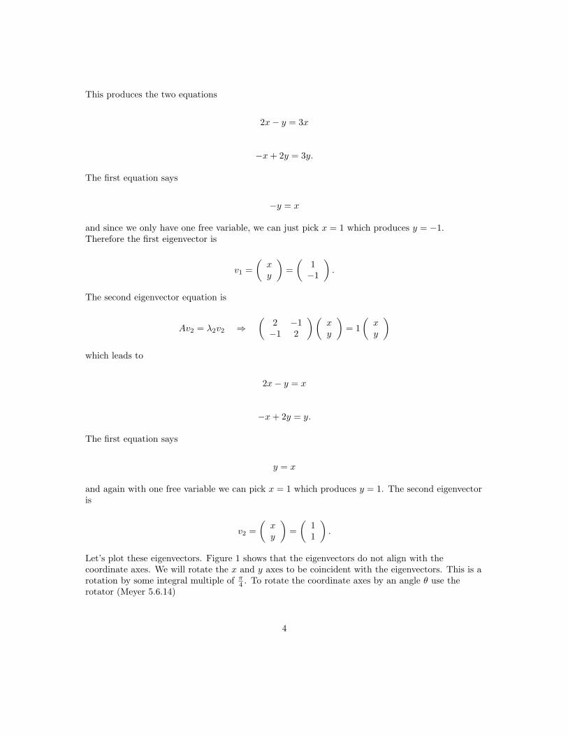
Let’s plot these eigenvectors. Figure 1 shows that the eigenvectors do not align with thecoordinate axes. We will rotate the x and y axes to be coincident with the eigenvectors. This is arotation by some integral multiple of π

4 . To rotate the coordinate axes by an angle θ use therotator (Meyer 5.6.14)

4

v1

v2

-1.0 -0.5 0.0 0.5 1.0

-1.0

-0.5

0.0

0.5

1.0

Figure 1: The two eigenvectors of A. The process of diagonalization is equivalent to aligning theeigenvectors with the coordinate axes.

P(θ) =(

cos θ − sin θsin θ cos θ

).

Recall that the rotator is an orthogonal operator. Let U be the operator which rotates thecoordinate axis through an angle -π4 .:

U =(

cos π4 sin π4− sin π

4 cos π4

)=

1√2

(1 1−1 1

).

The similarity transform is now

UTAU =1√2

(1 −11 1

)(2 −1−1 2

)( 1√2

)( 1 1−1 1

)=(

3 00 1

).

This transformation aligns v1 with the x-axis and v2 with the y-axis.

Call the diagonal matrix D and do a quick check of the reverse transformation:

UDUT =1√2

(1 1−1 1

)(3 00 1

)( 1√2

)( 1 −11 1

)=(

2 −1−1 2

). X

The MATLAB solution (see below) is

5

U =1√2

( −1 −1−1 1

)and the similarity transform is

UTAU =1√2

( −1 −1−1 1

)(2 −1−1 2

)( 1√2

)( −1 −1−1 1

)=(

1 00 3

).

This transformation aligns v1 with the y-axis and v2 with the x-axis.

11/6/07 5:27 PM MATLAB Command Window 1 of 1

EDU>> A=[2, −1; −1, 2] A = 2 −1 −1 2 EDU>> [U, D] = eig(A) U = −0.7071 −0.7071 −0.7071 0.7071 D = 1 0 0 3 EDU>> Uʼ’*A*U ans = 1.0000 0 0 3.0000

Figure 2: MATLAB results for the doagonalization.

6


1. Let

A =

(2 −1−1 2

).


[U,D] = eig(A) .

2. Let

A =

3 1 −1−1 1 1

2 2 0

.





A2 + A+ I = 0 .



A =

1 1 1 11 −1 1 0−1 0 0 1

0 −1 0 1−1 1 0 1

1 0 −1 1

.



| det(A) | = σ1σ2 . . . σn ?

1

2 Eigenvalues and diagonalization

The MATLAB poly command gave a list of four coefficients: {1, -4, 4, 0} which equates to acharacterisitic polynomial of

p(λ) = λ3 − 4λ2 + 4λ = 0

which factors as

λ(λ− 2)2 = 0

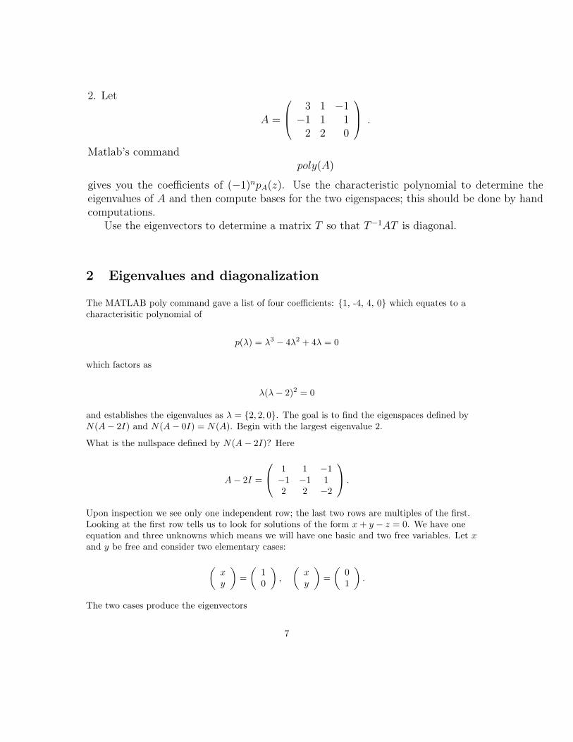
and establishes the eigenvalues as λ = {2, 2, 0}. The goal is to find the eigenspaces defined byN(A− 2I) and N(A− 0I) = N(A). Begin with the largest eigenvalue 2.

What is the nullspace defined by N(A− 2I)? Here

A− 2I =

1 1 −1−1 −1 12 2 −2

.

Upon inspection we see only one independent row; the last two rows are multiples of the first.Looking at the first row tells us to look for solutions of the form x+ y − z = 0. We have oneequation and three unknowns which means we will have one basic and two free variables. Let xand y be free and consider two elementary cases:

(xy

)=(

10

),

(xy

)=(

01

).

The two cases produce the eigenvectors

7

N(A− 2I) = sp{ 1

01

,

011

}.The 0 eigenvalue requires the resolution of

N(A) =

3 1 −1−1 1 12 2 0

.

For this simple system, we can find the nullspace quickly;

3 1 −1−1 1 12 2 0

xyz

=

000

leads to three equations

3x+ y − z = 0,

−x+ y + z = 0,

x+ y = 0.

The last line reveals that x+ y = 0 which means x = −y. Dropping this into the first equationyields 2x− z = 0 which implies z = 2x. For simplicity, pick x = 1. This makes y = −1 and z = 2.The result is

N(A) = sp{ 1

−12

}.At last we can build the transformation operator T

T =

1 0 10 1 −11 1 2

.

Next we need the inverse operator T−1. We’ll augment T with the identity matrix and reduce Tto the identity:

8

1 0 00 1 0−1 0 1

1 0 1 1 0 00 1 −1 0 1 01 1 2 0 0 1

=

1 0 1 1 0 00 1 −1 0 1 00 1 1 −1 0 1

,

1 0 00 1 00 −1 1

1 0 1 1 0 00 1 −1 0 1 00 1 1 −1 0 1

=

1 0 1 1 0 00 1 −1 0 1 00 0 2 −1 −1 1

,

1 0 00 1 00 0 1

2

1 0 1 1 0 00 1 −1 0 1 00 0 2 −1 −1 1

=

1 0 1 1 0 00 1 −1 0 1 00 0 1 − 1

2 − 12

12

,

1 0 −10 1 10 0 1

1 0 1 1 0 00 1 −1 0 1 00 0 1 − 1

2 − 12

12

=12

2 0 0 3 1 −10 2 0 −1 1 10 0 2 −1 −1 1

.

The inverse operator is

T−1 =12

3 1 −1−1 1 1−1 −1 1

.

The final step is to check the similarity transform:

T−1AT =12

3 1 −1−1 1 1−1 −1 1

3 1 −1−1 1 12 2 0

1 0 10 1 −11 1 2

=

2 0 00 2 00 0 0

. X

The careful student will check the reverse transformation on the diagonal matrix D:

TDT−1 =

1 0 10 1 −11 1 2

2 0 00 2 00 0 0

(12

) 3 1 −1−1 1 1−1 −1 1

=

3 1 −1−1 1 12 2 0

= A. X

In the last homework we plotted the transformation of the unit circle under a linear map. We canuse the same approach here to plot the distortion of the unit sphere under the map A. The figureshows that the unit sphere is smashed into an ellipse, The ellipse is a two-dimensional figure. Thedimension is the rank: rank(A) = 2.

9

Figure 3: Distortion of the unit sphere under the map A. The transformation surface has dimensionequal to the rank of A.

10

11/14/07 12:06 AM MATLAB Command Window 1 of 1

EDU>> A = [3 1 −1; −1 1 1; 2 2 0] A = 3 1 −1 −1 1 1 2 2 0 EDU>> poly(A) ans = 1.0000 −4.0000 4.0000 −0.0000 EDU>> [U, D] = eig(A) U = 0.8018 0.4082 −0.4877 −0.2673 −0.4082 0.8110 0.5345 0.8165 0.3233 D = 2.0000 0 0 0 0.0000 0 0 0 2.0000 EDU>> inv( U )*A*U ans = 2.0000 0.0000 −0.0000 0.0000 0.0000 −0.0000 0 0 2.0000

Figure 4: MATLAB results for the eigenvalue computation.

11

In[476]:= A = 883, 1, -1<, 8-1, 1, 1<, 82, 2, 0<<;% êê MatrixForm

Out[477]//MatrixForm=3 1 -1-1 1 12 2 0

In[478]:= poly = CharacteristicPolynomial@A, lD

Out[478]= -4 l + 4 l2 - l3

In[479]:= Solve@poly ã 0, lDOut[479]= 88l Ø 0<, 8l Ø 2<, 8l Ø 2<<

In[480]:= Eigensystem@ADOut[480]= 882, 2, 0<, 881, 0, 1<, 8-1, 1, 0<, 81, -1, 2<<<

In[487]:= T = Eigensystem@AD@@2DD¨;% êê MatrixForm

Out[488]//MatrixForm=1 -1 10 1 -11 0 2

In[489]:= Simplify@[email protected];% êê MatrixForm

Out[490]//MatrixForm=2 0 00 2 00 0 0

Zernike, MacOSX, 6.0 for Mac OS X x86 (32-bit) (June 19, 2007) Daniel M. Topa

/Users/dantopa/Documents/ nb 6/UNM/courses/math/514 Matrices/homework/01/514 hw 05 02.nb1 00:08:10, 11/14/07

Figure 5: Mathematica results for the eigenvalue computation.

12


1. Let

A =

(2 −1−1 2

).


[U,D] = eig(A) .

2. Let

A =

3 1 −1−1 1 1

2 2 0

.





A2 + A+ I = 0 .



A =

1 1 1 11 −1 1 0−1 0 0 1

0 −1 0 1−1 1 0 1

1 0 −1 1

.



| det(A) | = σ1σ2 . . . σn ?

1

3 Applying matrix analysis

By definition, a singular matrix has a determinant value of 0. This implies at least one eigenvalueis 0. If we can exclude a 0 eigenvalue or a 0 determinant we can prove that A is non-singular. Thetwo methods below rely on these facts.

3.1 Method 1: λ 6= 0

We start with the matrix equation

A2 +A+ I = 0.

We know that there is an eigenvalue relation

Ax = λx

for some x 6= 0. This leads directly to

A(Ax) = λ(λx).

The matrix equation can be recast as

(A2 +A+ I)x = (λ2 + λ+ 1)x = 0.

By assumption, x 6= 0 so the polynomial term must be 0:

λ2 + λ+ 1 = 0.

This polynomial equation does not have a 0 solution. Therefore A is not singular.

13

3.2 Method 2: factor the matrix equation

Start by factoring the matrix equation

A2 +A+ I = 0 ⇒ A(A+ I) = −I.

Take the determinant of both sides of the equation1

det(A(A+ I)

)= det(A)det(A+ I) = (−1)n.

Since the right-hand side is not 0, neither of the factors on the left-hand side can be 0. Thereforedet(A) 6= 0, therefore A cannot be singular.

1We thank P. Andrews for this proof.

14


1. Let

A =

(2 −1−1 2

).


[U,D] = eig(A) .

2. Let

A =

3 1 −1−1 1 1

2 2 0

.





A2 + A+ I = 0 .



A =

1 1 1 11 −1 1 0−1 0 0 1

0 −1 0 1−1 1 0 1

1 0 −1 1

.



| det(A) | = σ1σ2 . . . σn ?

1

4 Singular values and matrix rank

4.1 Rank of A

The matrix rank is clear when we have reduced A to row eschelon form. Here is a samplereduction where we have included multiple operations at some steps:

1 0 0 0 0 0−1 1 0 0 0 01 0 1 0 0 00 0 0 1 0 01 0 0 0 1 0−1 0 0 0 0 1

1 1 1 11 −1 1 0−1 0 0 10 −1 0 1−1 1 0 11 0 −1 1

=

1 1 1 10 −2 0 −10 1 1 20 −1 0 10 2 1 20 −1 −2 0

;

1 0 0 0 0 00 − 1

2 0 0 0 00 0 1 0 0 00 0 0 1 0 00 0 0 0 1 00 0 0 0 0 1

1 1 1 10 −2 0 −10 1 1 20 −1 0 10 2 1 20 −1 −2 0

=

1 1 1 10 1 0 1

20 1 1 20 −1 0 10 2 1 20 −1 −2 0

;

1 0 0 0 0 00 1 0 0 0 00 −1 1 0 0 00 1 0 1 0 00 −2 0 0 1 00 1 0 0 0 1

1 1 1 10 1 0 1

20 1 1 20 −1 0 10 2 1 20 −1 −2 0

=

1 1 1 10 1 0 1

20 0 1 3

20 0 0 3

20 0 1 10 0 −2 1

2

;

15

1 0 0 0 0 00 1 0 0 0 00 0 1 0 0 00 0 0 1 0 00 0 −1 0 1 00 0 2 0 0 1

1 1 1 10 1 0 1

20 0 1 3

20 0 0 3

20 0 1 10 0 −2 1

2

=

1 1 1 10 1 0 1

20 0 1 3

20 0 0 3

20 0 0 − 1

20 0 0 7

2

;

1 0 0 0 0 00 1 0 0 0 00 0 1 0 0 00 0 0 2

3 0 00 0 0 1

3 1 00 0 0 − 7

3 0 1

1 1 1 10 1 0 1

20 0 1 3

20 0 0 3

20 0 0 − 1

20 0 0 7

2

=

1 1 1 10 1 0 1

20 0 1 3

20 0 0 10 0 0 00 0 0 0

.

The matrix A has full rank: the rank r = n, the number of columns. In this case

rank(A) = 4.

4.2 Two ways to solve for eigenvalues

In the last homework we saw that we had two choices for finding the singular values: compute theeigenvalues of WU = AAT or compute the eigenvalues of WV = ATA. The solutions said that thesmaller matrix would be easier to work with. Let’s look at the dimensions of the matrices involvedwith computing the singular values:

A : 6× 4AT : 4× 6AAT : 6× 6ATA : 4× 4

.

Specifically the two product matrices are

WU = AAT =

4 1 0 0 1 11 3 −1 1 −2 00 −1 2 1 2 00 1 1 2 0 11 −2 2 0 3 01 0 0 1 0 3

,

with the 6th order chracteristic polynomial pWU(A) = λ6 − 17λ5 + 104λ4 − 270λ3 + 251λ2 and

16

WV = ATA =

5 −1 1 0−1 4 0 11 0 3 00 1 0 5

.

with the 4th order chracteristic polynomial pWV(A) = λ4 − 17λ3 + 104λ2 − 270λ+ 251. The

polynomial equations are equivalent. We see that

pWV(λ) = λ2pWU

(λ)

so the six roots of pWU(A) will be the four roots of pWV

(A) augmented with two zeros. In termsof polynomial complexity there is no advantage to using either WV or WU . However, the smallermatrix is much easier to work with to find the eigenvalues.

The four roots of the characteristic polynomial equation

pWv(A) = λ4 − 17λ3 + 104λ2 − 270λ+ 251 = 0

are the eigenvalues we want. The roots are

λ1,2 =12

√17 + 2β ±

√γ

3+

1β,

λ3,4 =12

√17− 2β ±

√γ

3− 1β,

where

α = 3

√12

(853 + 3i

√5871

), β =

√α

3+

3512

+583α, γ = −4α+ 70− 232

α.

4.3 The singular values

The singular values σ are the magnitudes of the eigenvalues

σ = ‖λ‖2.

Since the eigenvalues are complex the modulus is

σi = λiλi.

In numeric form the singular values are

17

5.12 Singular Value Decomposition 417

Solution: Without realizing it, we answered this question in Example 5.12.1.To bound the accuracy of x̃ relative to the exact solution x, write r = b−Ax̃as Ax̃ = b− r, and apply (5.12.8) with e = r to obtain

κ−1 ‖r‖2‖b‖2

≤ ‖x− x̃‖‖x‖ ≤ κ

‖r‖2‖b‖2

, where κ = ‖A‖2∥∥A−1

∥∥2. (5.12.9)

Therefore, for a well-conditioned A, the residual r is relatively small if andonly if x̃ is relatively accurate. However, as demonstrated in Example 5.12.1,equality on either side of (5.12.9) is possible, so, when A is ill conditioned, avery inaccurate approximation x̃ can produce a small residual r, and a veryaccurate approximation can produce a large residual.Conclusion: Residuals are reliable indicators of accuracy only when A is wellconditioned—if A is ill conditioned, residuals are nearly meaningless.

In addition to measuring the distortion of the unit sphere and gauging thesensitivity of linear systems, singular values provide a measure of how close Ais to a matrix of lower rank.

Distance to Lower-Rank MatricesIf σ1 ≥ σ2 ≥ · · · ≥ σr are the nonzero singular values of Am×n, thenfor each k < r, the distance from A to the closest matrix of rank k is

σk+1 = minrank(B)=k

‖A−B‖2. (5.12.10)

Proof. Suppose rank (Bm×n) = k, and let A = U(

D 00 0

)VT be an SVD

for A with D = diag (σ1, σ2, . . . , σr) . Define S = diag (σ1, . . . , σk+1), andpartition V =

(Fn×k+1 |G

). Since rank (BF) ≤ rank (B) = k (by (4.5.2)),

dimN (BF) = k+1−rank (BF) ≥ 1, so there is an x ∈ N (BF) with ‖x‖2 = 1.Consequently, BFx = 0 and

AFx = U(

D 00 0

)VTFx = U

S 0 00 � 00 0 0

x00

= U

Sx00

.

Since ‖A−B‖2 = max‖y‖2=1 ‖(A−B)y‖2 , and since ‖Fx‖2 = ‖x‖2 = 1(recall (5.2.4), p. 280, and (5.2.13), p. 283),

‖A−B‖22 ≥ ‖(A−B)Fx‖22 = ‖Sx‖22 =k+1∑i=1

σ2i x

2i ≥ σ2

k+1

k+1∑i=1

x2i = σ2

k+1.

Equality holds for Bk = U(

Dk 00 0

)VT with Dk = diag (σ1, . . . , σk), and thus

(5.12.10) is proven.

Figure 6: Meyer, page 417, shows how the singular values specify the distance from A to the nearestmatrices of lower ranks.

σ1 = 2.47523σ2 = 2.27972σ3 = 1.80348σ4 = 1.55679

.

As Meyer shows (see above) the distance from a matrix A to the closest matrix of rank k is σk+1.For example, the distance from A to the nearest rank 3 matrix is σ4. The table below shows thedistances from A to the nearest ...

rank 1 matrix: σ2 = 2.27972rank 2 matrix: σ3 = 1.80348rank 3 matrix: σ4 = 1.55679

.

18


1. Let

A =

(2 −1−1 2

).


[U,D] = eig(A) .

2. Let

A =

3 1 −1−1 1 1

2 2 0

.





A2 + A+ I = 0 .



A =

1 1 1 11 −1 1 0−1 0 0 1

0 −1 0 1−1 1 0 1

1 0 −1 1

.



| det(A) | = σ1σ2 . . . σn ?

1

5 The singular value decomposition - again

How do we relate the determinant to singular values? We need the singular values and these comefrom the SVD

A = UΣV ∗

where all the component matrices have the same dimension as A: n× n. Use the product rule fordeterminants:

|det(A)| = |det(UΣV ∗)| = |det(U)||det(Σ)||det(V ∗)|.

What is the determinant of a unitary matrix? To answer this we need to relate the determinant ofa matrix B to the determinant of of the complex conjugate B̄. As we saw in lecture, in the coursenotes (p. 34) and Meyer (see below) the determinant is defined in terms of permutations of thematrix elements as

det(B) =∑σ∈SN

sgn(σ)bσ11 . . . bσnn.

What happens to the determinant when we take the complex conjugate of the matrix elements?That is when

bij ⇒ b̄ij .

The product of complex conjugates is the complex conjugate of the product:

b̄σ11 . . . b̄σnn ⇒ bσ11 . . . bσnn

and sum of complex conjugates is the complex conjugate of the sum:

∑σ∈SN

sgn(σ)bσ11 . . . bσnn ⇒∑σ∈SN

sgn(σ)bσ11 . . . bσnn.

Therefore

19

6.1 Determinants 461

also be even (odd). Accordingly, the sign of a permutation p is defined to bethe number

σ(p) =

+1 if p can be restored to natural order by an

even number of interchanges,−1 if p can be restored to natural order by an

odd number of interchanges.

For example, if p = (1, 4, 3, 2), then σ(p) = −1, and if p = (4, 3, 2, 1), thenσ(p) = +1. The sign of the natural order p = (1, 2, 3, 4) is naturally σ(p) = +1.The general definition of the determinant can now be given.

Definition of DeterminantFor an n× n matrix A = [aij ], the determinant of A is defined tobe the scalar

det (A) =∑

p

σ(p)a1p1a2p2 · · · anpn , (6.1.1)

where the sum is taken over the n! permutations p = (p1, p2, . . . , pn)of (1, 2, . . . , n). Observe that each term a1p1a2p2 · · · anpn

in (6.1.1) con-tains exactly one entry from each row and each column of A. The de-terminant of A can be denoted by det (A) or |A|, whichever is moreconvenient.Note: The determinant of a nonsquare matrix is not defined.

For example, when A is 2× 2 there are 2! = 2 permutations of (1,2),namely, {(1, 2) (2, 1)}, so det (A) contains the two terms

σ(1, 2)a11a22 and σ(2, 1)a12a21.

Since σ(1, 2) = +1 and σ(2, 1) = −1, we obtain the familiar formula∣∣∣∣ a11 a12

a21 a22

∣∣∣∣ = a11a22 − a12a21. (6.1.2)

Example 6.1.1

Problem: Use the definition to compute det (A), where A =(

1 2 34 5 67 8 9

).

Solution: The 3! = 6 permutations of (1, 2, 3) together with the terms in theexpansion of det (A) are shown in Table 6.1.1.

Figure 7: Meyer, page 461, defines the determinant in terms of permutations. This notation issimilar to the notation used in lecture.

det(B̄) = det(B).

We already know that det(BT ) = det(B) so we can now relate the determinants of B and B∗:

det(B∗) = det(B).

For the unitary matrix U we know UU∗ = I. In terms of determinants we have

det(UU∗) = det(I) = 1.

From this we conclude

det(UU∗) = det(U)det(U∗) = det(U)det(U) = |det(U)|2 = 1.

This shows that det(U) has unit modulus when U is unitary.

Returning to the determinant equation we see that since U and V ∗ are unitary

|det(U)| = 1, |det(V ∗)| = 1.

The product rule we started with is

|det(A)| = |det(U)||det(Σ)||det(V ∗)| = |det(Σ)|.

20

Because Σ is a diagonal matrix

det(Σ) =n∏i=1

σi

The last question to address is whether or not

n∏i=1

σi = σ1σ2 . . . σn = |σ1σ2 . . . σn|?

The answer is yes because the singular values are greater than or equal to 0.

21