i a a p - h q . o r g

Professional Secrets in Excel Neil Malek

Building a spreadsheet has many facets - data entry, formatting, calculations, and

reporting included - and you’ve probably met someone who somehow does it all better

than you. In this session, we’ll cover shortcuts and tools the pros use every day to make

their work better and faster. We’ll pull back the curtain on things like nested functions, named ranges, tables, and data validation.

CONTENTSNAMED RANGES

UNDERSTANDING NAMED RANGES 3

CREATING A SIMPLE NAMED RANGE 4

UPDATING A NAMED RANGE 5

USING TABLE RANGES 6

DATA VALIDATION

UNDERSTANDING DATA VALIDATION 8

RANGE-BASED VALIDATION 8

DATA CLEAN-UP

LEFT AND FIND 10

TRIM AND PROPER 11

TODAY AND NETWORKDAYS 12

LOOKUP FUNCTIONS

VLOOKUP 13

INDEX AND MATCH 14

LOGICAL FUNCTIONS

IF 15

IFERROR 17

SUMIFS 19

MAPPING TABLES 21

Perfect PDFs

Neil Malek

iaap-hq.org 2

NAMED RANGESUNDERSTANDING NAMED RANGESWhen calculating values in Excel, our functions and formulas rely on references to other cells in order to complete their job. For example, =SUM(B4:B17) in this screenshot.

However, constantly referring to cells by their location (B4) means that you (1) are repeating yourself very frequently, (2) must update every reference to B4 if the calculation changes, and (3) have absolutely no additional information or assistance in getting thing done. B4 just doesn’t tell you anything about what is happening in that cell, and why you’re referring to it.

By creating a named range, you create a permanent reference that can be reused and updated in a central location, and that has a name you can use for context. There are a different techniques to creating named ranges that give you additional benefits, but they all share those simple reasons.

Perfect PDFs

Neil Malek

iaap-hq.org 3

CREATING A SIMPLE NAMED RANGEThe standard named range is created by using the following steps

(1) Select the appropriate cell(s). In this example, I’ve highlighted a value that will be used as the Depreciation Rate for a number of assets (G2).

(2) Click within the Name Box. The Name Box is the small box below the Ribbon on the far left side of the screen, just above the spreadsheet. You’ll notice this always has the cell name listed (G2 here).

(3) Enter a valid and useful name for the cell(s). Valid means that it’s a name that does not have spaces in it - Excel doesn’t like spaces in named items. Useful just means that the name will mean something to you later. I’ve typed DepreciationRate - notice the capital D and R to make the words easier to distinguish.

Perfect PDFs

Neil Malek

iaap-hq.org 4

UPDATING A NAMED RANGEMoving the reference of a named range from one cell (or group of cells) to another is one of the most useful features of named ranges. If, for example, you need to move from the 2016 Commission Rate to the 2017 Commission Rate, simply click Formulas Tab > Name Manager.

Now, select the named range you need to update (CommissionRate), and choose Edit...

Update your named range from, say, $H$6 to $H$7, and watch all the functions that use that reference adjust to the new values.

Perfect PDFs

Neil Malek

iaap-hq.org 5

USING TABLE RANGESA common occurrence in Excel files is referencing a column of cells that have similar information - like taking the SUM of the TRANSACTION VALUE column in this spreadsheet. The biggest issue with this reference is that you will find yourself adding more values to the column, and you’d like a reference to reflect the current state of the spreadsheet.

To do this, we select the set of cells to be converted (click on one of the cells within the range), and choose Insert Tab > Table.

Perfect PDFs

Neil Malek

iaap-hq.org 6

This will ask you if it’s successfully selected all the relevant cells, and if your data has headers.

As a final step, you should also choose Table Tools Tab > Table Name Box and type a custom name (like Transactions) that you will recognize later.

Now, when you choose to use the SUM function on the TRANSACTION VALUE column, the reference is to Transactions[Transaction Value], which is the name of the table and the name of the column. As the table changes size, your reference will update to include only the relevant cells.

Perfect PDFs

Neil Malek

iaap-hq.org 7

DATA VALIDATIONUNDERSTANDING DATA VALIDATIONIf you open a new spreadsheet, each cell within that file is completely unprotected. Any user can enter any information into any cell, with no restrictions. We’ll discuss putting passwords onto these cells later, but this section of the handout is devoted to Data Validation, the restriction of the type of information you can enter.

With Data Validation, you can restrict the possible data entered into a cell to a date format, number format, or even one options from a list.

On the final panel of your Data Validation, you decide whether to Stop your users from entering an invalid value, or just Warn or give them Information.

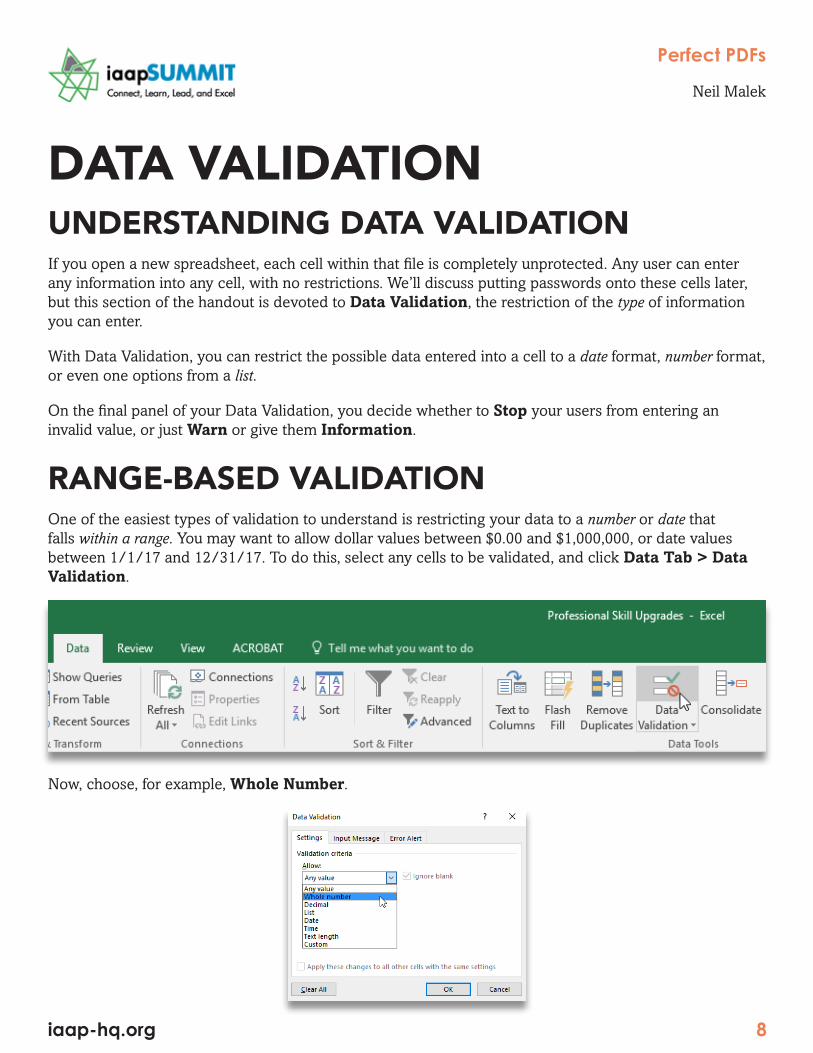
RANGE-BASED VALIDATIONOne of the easiest types of validation to understand is restricting your data to a number or date that falls within a range. You may want to allow dollar values between $0.00 and $1,000,000, or date values between 1/1/17 and 12/31/17. To do this, select any cells to be validated, and click Data Tab > Data Validation.

Now, choose, for example, Whole Number.

Perfect PDFs

Neil Malek

iaap-hq.org 8

Enter a Minimum and Maximum for the range.

At this point, move over to the Error Alert Tab and choose the option that most fits your situation (to require the value fall within the range, choose Stop to stop anything other than the correct values, and to allow users to enter things that don’t fall within the range with a warning message, choose Warning for a stronger message, and Information for a weaker message. Fill in the text as you like.

Perfect PDFs

Neil Malek

iaap-hq.org 9

DATA CLEAN-UPLEFT AND FINDWhenever we want to get someone’s first name, city, state, zip, or other bit of information from a larger cell full of information, we need to use the FIND function, nested into LEFT, RIGHT, or MID.

Let’s start with LEFT, RIGHT, and MID. LEFT starts from the left side of your text, and grabs as much of the content as you like. For example, the function below would return Daytona Beach.

However, it wouldn’t work for the other pieces of information, because each city has a different number of characters. This is where the FIND function comes in.

FIND has one job - it finds the position of whatever character you want. So, for example, you could use the FIND function to determine that the comma in Daytona Beach, FL 32114 was the 14th position.

Combine these together - LEFT using FIND to determine the location of the comma - and subtract 1 in order to not include the comma. You’ve got a nested function that can pull data apart.

Perfect PDFs

Neil Malek

iaap-hq.org 10

TRIM AND PROPERPoor capitalization and extra spaces are a common, sloppy data entry issue. There are three capitalization functions - UPPER, LOWER, and PROPER - that will change how the content is capitalized.

To remove leading or following spaces - not the spaces between text - simply put the content into the TRIM function.

Perfect PDFs

Neil Malek

iaap-hq.org 11

TODAY AND NETWORKDAYSTo dynamically create the current date, simply use the =TODAY() function (the keyboard shortcut to enter a static function is [CTRL] + [;]).

Subtracting dates is simple enough, but that functionality doesn’t reflect weekends and holidays. The NETWORKDAYS function automatically subtracts weekend days, and if you create an array of holidays your organization recognizes, it subtracts those values as well.

Perfect PDFs

Neil Malek

iaap-hq.org 12

LOOKUP FUNCTIONSVLOOKUPVLOOKUP is a structured vertical lookup function - if your data is arranged vertically (as below), you can find a match for some value.

The structure of the function is as follows: you provide the full set of data you’re using for the lookup, and VLOOKUP automatically looks in the first (leftmost) column of that data for your match. Because of that structure, many professionals move toward a more flexible arrangement with INDEX and MATCH (next segment).

Into the VLOOKUP function, enter what your looking for (BANK ID), where you’re looking (A4:D6), and which column you want back (REPRESENTATIVE, column number 3). Finally, if you’re looking for an exact match, always end with the word FALSE.

Perfect PDFs

Neil Malek

iaap-hq.org 13

INDEX AND MATCHINDEX and MATCH are a more flexible replacement for VLOOKUP, because while VLOOKUP always looks in the first column for the match, and you enter a column index number to retrieve a specific result, INDEX uses the MATCH function to constantly calculate where the data you want is.

Begin by entering the INDEX function and providing it with the data table you’re interested in:

Now, to provide the input about which row to return, use the MATCH function to find a match for the Seller Code in the second column:

(In this example, the 0 value means you want an exact match)

Then, you can either enter the column number of the data you want to return, or you can use a second MATCH function to find the column you want:

Perfect PDFs

Neil Malek

iaap-hq.org 14

LOGICAL FUNCTIONSIFThe ultimate true/false function is a critical element of professional Excel use. In this example, I’m using it to highlight whether the director needs to be concerned about an event. To judge whether they should be concerned, we’ll take the Current Event Score compared against 75, and the Event Date compared against today’s date. If the score is below 75, and the event date is fewer than 365 days away, the director should be concerned.

Select cell P4, and click Formulas Tab > Logical Drop-Down > IF.

Into the Logical Test box, you need to compare two things. This requires the AND function. Type AND( into the box.

Perfect PDFs

Neil Malek

iaap-hq.org 15

Now, your two comparisons are (1) is the Current Event Score below 75? and (2) is the Event Date sooner than TODAY()+365? For the first one, type O4<=75.

Type a comma after the first comparison, and type A4<=TODAY()+365. Don’t worry when Excel tells you this is Volatile - that’s just because you always need to know what TODAY is before you can tell whether it’s true or not.

Now, we need to know - is the score below 75, and it’s within one year of the event? If so - enter into the Value if True box and add a value that means things are going badly - I’m typing “Attention Required”. If they aren’t true, then something like “No Issue” will go into the Value if False box.

Perfect PDFs

Neil Malek

iaap-hq.org 16

IFERRORWhile the IF function can evaluate anything TRUE or FALSE, there’s a specific situation you should be able to handle, and Microsoft has given us a more specific tool to deal with it. The situation is handling functions that sometimes evaluate to error messages. First, an example:

As you can see, each of these functions - sum, average, max, and min - all point at the same set of cells that are currently empty. However, only one of them gives you a problem. Averages use division, and since there aren’t any values to divide, you get a DIV/0 error.

It’s relatively simple to see that you want the average function to work the same as the others - if there aren’t any values, just produce a 0, and we can move on. This a scenario that calls for the IFERROR function.

Choose the cell you want your AVERAGE or VLOOKUP (the other very common scenario) in, and choose Formulas Tab > Logical Drop-Down > IFERROR.

Perfect PDFs

Neil Malek

iaap-hq.org 17

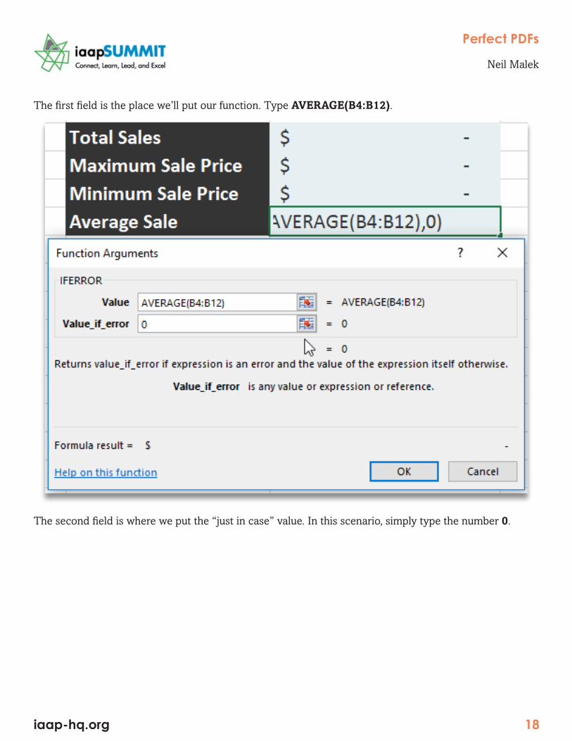
The first field is the place we’ll put our function. Type AVERAGE(B4:B12).

The second field is where we put the “just in case” value. In this scenario, simply type the number 0.

Perfect PDFs

Neil Malek

iaap-hq.org 18

SUMIFSConditional summing helps build reports much more quickly than the alternative. Excel has both SUMIF and SUMIFS, with SUMIFS being the most recent addition to the program. SUMIFS is the function that has multiple criteria available, while SUMIF only has one possible criteria.

One use of SUMIFS is in mapping multiple tables together; in this example, you can add up all the sales of each Sales Representative from the Raw Data table very easily - or each Customer, Customer Type, Region, Product, or Product Class. In cell I6, click Formulas Tab > Math and Trig > SUMIFS.

Perfect PDFs

Neil Malek

iaap-hq.org 19

For Sum Range, refer to the column with the Sale Price. In my spreadsheet, that ends up being SalesTable[Sale Price].

For the Criteria Range, refer to the cells that have the Sales Representative in them - again, my spreadsheet has SalesTable[Sales Representative].

Finally, give the Criteria that this is compared against - cell G6, or as you can see in my spreadsheet RegionTable[@[Sales Representative].

Perfect PDFs

Neil Malek

iaap-hq.org 20

MAPPING TABLESExcel is often used to hold large sets of data, blurring the line with database tools like Access, SQL Server, Oracle, and others. If you’re tracking large tables of information in Excel, you should adhere to the rules that database professionals use when using real database software. One of the most important rules is to avoid duplicated and non-uniform data. As an example, you might find entries like these in a spreadsheet:

You can tell that these are probably supposed to be the same thing, but aren’t. This is going to cause problems in the future, as we try to summarize the data, and Excel doesn’t recognize them as being the same category.

Perfect PDFs

Neil Malek

iaap-hq.org 21

One tool we can use to solve this issue is to map tables in Excel. Instead of tying all the data you have to a huge data set, break it down. As you can see in this screenshot, we might start with a table that has all the information about the customer, sales person, and product ‘under one roof ’.

Instead, by breaking the information into multiple tables: a table for the transaction, one for the customer, one for the sales person, and one for the product, we can maintain flexibility. Imagine there’s a shake-up in the Sales Department, and different sales people report to different managers. With the new independent sales person table, you can quickly update that information.

Now, you can use these mappings in multiple ways. One is to add a SUMIFS function to the mapped sales person table, to combine the total sales of each sales person.

Then, you can add another mapping table, putting each of the managers into regions.

Perfect PDFs

Neil Malek

iaap-hq.org 22