NBER WORKING PAPER SERIES

PROFESSIONALS DO NOT PLAY MINIMAX:EVIDENCE FROM MAJOR LEAGUE BASEBALL AND THE NATIONAL FOOTBALL LEAGUE

Kenneth KovashSteven D. Levitt

Working Paper 15347http://www.nber.org/papers/w15347

NATIONAL BUREAU OF ECONOMIC RESEARCH1050 Massachusetts Avenue

Cambridge, MA 02138September 2009

¸˛We are grateful to John List, Ben Baumer, Andrew Stein, Jeff Ma, Mark Kamal, Lucas Ruprecht,and Paraag Marathe for helpful comments and discussions. Daniel Hirschberg provided outstandingresearch assistance. Thanks to Baseball Info Solutions and Citizen Sports Network for providing data. Correspondence should be addressed to: Professor Steven Levitt, Department of Economics, Universityof Chicago, 1126 E. 59th Street, Chicago, IL 60637, or slevitt@uchicago.edu. The views expressedherein are those of the author(s) and do not necessarily reflect the views of the National Bureau ofEconomic Research.

NBER working papers are circulated for discussion and comment purposes. They have not been peer-reviewed or been subject to the review by the NBER Board of Directors that accompanies officialNBER publications.

© 2009 by Kenneth Kovash and Steven D. Levitt. All rights reserved. Short sections of text, not toexceed two paragraphs, may be quoted without explicit permission provided that full credit, including© notice, is given to the source.

Professionals Do Not Play Minimax: Evidence from Major League Baseball and the NationalFootball LeagueKenneth Kovash and Steven D. LevittNBER Working Paper No. 15347September 2009JEL No. D01,D82

ABSTRACT

Game theory makes strong predictions about how individuals should behave in two player, zero sumgames. When players follow a mixed strategy, equilibrium payoffs should be equalized across actions,and choices should be serially uncorrelated. Laboratory experiments have generated large and systematicdeviations from the minimax predictions. Data gleaned from real-world settings have been more consistentwith minimax, but these latter studies have often been based on small samples with low power to reject.In this paper, we explore minimax play in two high stakes, real world settings that are data rich: choiceof pitch type in Major League Baseball and whether to run or pass in the National Football League.We observe more than three million pitches in baseball and 125,000 play choices for football. Wefind systematic deviations from minimax play in both data sets. Pitchers appear to throw too manyfastballs; football teams pass less than they should. In both sports, there is negative serial correlationin play calling. Back of the envelope calculations suggest that correcting these decision making errorscould be worth as many as two additional victories a year to a Major League Baseball franchise, andmore than a half win per season for a professional football team.

Kenneth KovashMozilla 5807 S Woodlawn AveChicago, IL 60637kkovash@gmail.com

Steven D. LevittDepartment of EconomicsUniversity of Chicago1126 East 59th StreetChicago, IL 60637and NBERslevitt@midway.uchicago.edu

A spirited debate has arisen regarding the question of the extent to which actions

in two-player zero sum games conform to the predictions of game theory. Von

Neumann’s Minimax theory makes three basic predictions about behavior in such games.

First, since the player must be indifferent between actions in order to mix, the expected

payoffs across all actions that are part of the mixing equilibrium must be equalized.

Second, the expected payoff for all actions that are played with positive probability must

be greater than the expected payoff for all actions that are not played with positive

probability.2 Third, the choice of actions is predicted to be serially independent, since if

the pattern of play is predictable, it can be exploited by an optimizing opponent.

Laboratory tests of minimax have, almost without exception, shown substantial

deviations from these theoretical predictions (Lieberman, 1960,1962; Brayer 1964,

Messick 1967, Fox 1972, Brown and Rosenthal 1990, Rosenthal et al. 2003). One

remarkable exception to this pattern is Palacios-Huerta and Volij (2008), in which soccer

players who are brought into the laboratory play minimax in both a 2x2 game and

O’Neill’s (1987) 4x4 game. Levitt, List, and Reiley (2008), however, are unable to

replicate these findings, either using professional soccer players or world class poker

players, calling the Palacios-Huerta and Volij results into question.

In stark contrast to the lab, the existing literature on minimax play in the field has

generally provided support to the predictions of game theory. Whether the task is the

direction of a serve in tennis (Walker and Wooders 2001, Hsu, Huang, and Tang 2007),

2 In most prior empirical analyses, this prediction has either been irrelevant of untestable. If there are only two actions available (e.g. Walker and Wooders 2001, Hsu, Huang, and Tang 2007), then by definition any mixing strategy must include both actions. Even when the action space is richer, the expected payoff to an action that is not taken is typically not observed, making this prediction untestable. Hirschberg, Levitt, and List (2009), on the other hand, are able to address this prediction in studying the actions of poker players because of the richness of their data.

penalty kicks in soccer (Chiappori, Levitt, and Groseclose 2002, Palacios-Huerta 2003),

or the decision to call, check, fold, or raise in limit poker (Hirschberg et al. 2009),

equalized payoffs across actions that are included in the mixed strategy cannot be

rejected. The evidence on serial independence in the field is more mixed, but has found

some support (e.g., Hsu, Huang, and Tang 2007).

There are a number of possible explanations for the sharp differences observed in

prior studies done in the laboratory versus the field. Failure of minimax in the lab may

be the result of a lack of familiarity with the games that are played, low stakes, or

selection of participants into the studies who do not have experience or talent for mixing.

A very different explanation for the contrasting conclusions of lab and field studies is that

field studies tend to have very low power to reject (Levitt and List 2007). For instance,

in Chiappori, Levitt, and Groseclose (2002), the total number of penalty kicks is only

459, spread over more than 100 shooters. Walker and Wooders (2001) observe

approximately 3,000 serves spread over forty Grand Slam tennis matches.

In this paper, we add to the existing literature by studying behavior in two new

field settings: the pitcher’s choice of pitch type (e.g., fastball versus curveball) in

professional baseball, and the offense’s choice of run versus pass in professional football.

In each of these settings, we are able to analyze far more data than has previously been

available in field studies of mixed strategy behavior. In the case of baseball, we observe

every pitch thrown in the major leagues over the period 2002-2006 – a total of more than

3 million pitches. For football, we observe every play in the National Football League

for the years 2001-2005 – over 125,000 plays. In both settings, the choices being made

have very high stakes associated with them.

The results obtained from analyzing the football and baseball data are quite

similar. In both cases, we find clear deviations from minimax play, as evidenced by a

failure to equalize expected payoffs across different actions played as part of mixed

strategies, and with respect to negative serial correlation in actions. In the NFL, we find

that offenses on average do systematically better by passing the ball rather than running.

In baseball, pitchers appear to throw too many fastballs, i.e., batters systematically have

better outcomes when thrown fastballs versus any other type of pitch.

In football, teams are more likely to run if the previous play was a pass, and vice

versa. This pattern is especially pronounced when the previous play was unsuccessful.

Negative serial correlation in actions is consistent with a large body of prior laboratory

evidence (e.g., Brown and Rosenthal 1990). Pitchers also exhibit some negative serial

correlation, particularly with fastballs, i.e., they are more likely to throw a non-fastball if

the previous pitch was a fastball, and vice versa.

The magnitude of these deviations is not trivial. Back-of-the-envelope

calculations suggest that the average NFL team sacrifices one point a game on offense

(4.5 percent of current scoring) as a consequence of these mistakes. In baseball, we

estimate that the average team gives up an extra 20 runs a season (about a 1.3 percent

increase). If these estimates are correct, then the value to improving these decisions is on

the order of $4 million a year for the typical baseball team and $5 million a year for an

NFL franchise.

The remainder of the paper is structured as follows. Section I reports our results

for major league baseball. Section II analyzes NFL football. Section III concludes.

Section I: An analysis of pitch choice in major league baseball

Our data on pitch choice in major league baseball were purchased from Baseball

Info Solutions, which employs data trackers at all games and compiles the information in

order to sell it to major league teams and other interested parties. The data set includes a

wealth of information for each pitch thrown in the major leagues over the period 2002-

2006: the identity of the pitcher and batter, the current game situation (inning, count,

number of outs, current score, etc.), the type of pitch thrown, and the outcome of the

pitch (e.g., home run, foul, sacrifice bunt).

There are multiple dimensions along which pitches vary: the type of pitch (e.g.,

changeup, slider, fastball), the location of the pitch, the velocity, etc. We limit our

attention to just one of these dimensions: pitch type.3 The raw data contain 12 different

types of pitches. After consultation with major league teams, we consolidated these into

five categories: fastball, curveball, slider, changeup, and other.4 In our analysis, we drop

all pitches classified as “other.”5

Our primary outcome measure for an at bat is the baseball statistic known as

“OPS,” which is the sum of a batter’s on-base percentage and his slugging percentage. In

3 Unlike velocity or location, pitch type is not affected by faulty execution on the part of the pitcher; a pitcher might intend to locate a pitch over the inside corner of the plate, but mistakenly throw it to the outside of the plate. 4 These pitch types, with number of cases in parentheses, are as follows: Fastballs (2,083,248) and cut fastballs (39,830) are combined as “fastball.” Changeups (362,387) and split fingers (50,818) are combined as “changeup.” Forkballs (430), knuckleballs (18,905), pitchouts (4,379), screwballs (766), sinkers (84), and unknowns (188,927) are combined as “other.” Sliders (449,378) and curveballs (314,633) compose the rest of the data. 5 The accuracy with which pitch type is coded is critical to our study. As a check on this issue, we obtained the coding for an overlapping sample of pitches collected by STATS Inc., which competes with Baseball Info Solutions in providing information to baseball teams. These two independent assessments of pitch type match on over 90 percent of all pitches. The coding matches especially well on fastballs, with more variation occurring when the two data sets code an off-speed pitch differently. If we limit our comparison to fastball versus non-fastball, approximately 94 percent of all pitch types match across the two data sets. Importantly, the degree to which the two data sets match does not appear to be a function of the outcome of the at bat. Match rates are nearly identical regardless of whether the pitch is not put in play, is put in play for a hit, or is put in play for an out.

prior empirical research, OPS has been shown to be a strong predictor of the number of

runs a team scores (Fox 2006). If a batter makes an out, his OPS for that at bat is zero. If

the batter walks, his OPS is one. A single earns an OPS of two, a double an OPS of

three, a triple an OPS of four, and a home run an OPS of five.

Our raw data covers every regular season pitch thrown in the major leagues over

the period 2002-2006. After generating season level statistics such as batter OPS, we

exclude any at bat including any pitch categorized as “other,” as well as data from extra

innings. After these exclusions, we have 3,110,429 total pitches thrown. Table 1

presents summary statistics for these pitches. As shown in column 1, fastballs are the

most common type of pitch, accounting for approximately 65 percent of all throws.

Sliders are the second most common pitch type, followed by changeups and curveballs.

Columns 2-5 of Table 1 report the distribution of outcomes for each pitch type.

We report four mutually exclusive and exhaustive pitch outcomes: a ball, a strike, the ball

is put into play and the batter is out, and the ball is put into play and the batter gets a hit.6

Pitchers are slightly more likely to record strikes when throwing fastballs relative to all

non-fastballs, and slightly less likely to register a ball. Changeups are most likely to lead

to both an out (15.29 percent) and a hit (7.08 percent); curveballs are least likely to yield

both outs and hits. Column 6 of Table 1 shows the OPS (our preferred outcome metric)

by pitch type when the pitch ends the at bat. Foreshadowing the results from the

regression analysis, the OPS on fastballs is higher than for non-fastballs: .753 versus

.620. One potential explanation for that gap, however, is that fastballs are more likely to

be thrown in hitters’ counts, as demonstrated in the final three columns of Table 1.

6 A foul ball that is not caught for an out is classified as a strike in this categorization.

To further explore the role of the count, Table 2 reports results for pitches thrown

on each possible count, e.g., 1-0, 3-1, etc. As column 3 demonstrates, the likelihood of a

fastball varies widely across counts. On a 3-0 count, almost 95 percent of all pitches are

fastballs; when the count is 1-2 the share of fastballs is only 52 percent. Columns 3-6

show OPS comparisons for fastballs and non-fastballs by count, for pitches that end the at

bat. The differences in outcomes for fastballs versus non-fastballs tend to be small when

there are fewer than two strikes. On two strike counts, however, non-fastballs generate

an OPS that is more than 100 points lower than for fastballs, and this gap is highly

statistically significant. The last four columns of Table 2 report the final outcome of the

at-bat as a function of which pitch was thrown at each count, when that pitch does not

actually end the at-bat. If there are no spillovers across pitches, there should be no

difference in outcomes across pitch types if the pitch does not end the at bat. To the

extent, however, that fastballs are slightly more likely to generate strikes than non-

fastballs, throwing a fastball may provide some benefit to the pitcher when the at-bat

does not end with the current pitch. 7 The results in the last four columns of Table 2

suggest, however, that, if anything, throwing a fastball on the current pitch leads to

slightly worse outcomes within this at-bat if the pitch does not terminate the at-bat. For

most counts, the eventual at-bat OPS is close for fastballs and non-fastballs, but with two

strikes the non-fastballs yield lower OPS.

7 There are other channels, as well, via which a fastball might provide deferred benefits. First, it may be that it is harder to hit a pitch if the preceding pitch was a fastball. Second, fastballs might be less likely to generate other negative results, like wild pitches, passed balls, and stolen bases. Third, fastballs might cause less wear and tear on the pitcher’s arm. Back of the envelope calculations suggest that none of these channels is likely to be even close to a magnitude to offset the observed OPS differences between fastballs and other pitches.

Table 3 analyzes more formally the link between pitch type and OPS using

regression specifications of the following form:

(1) 'apb k apb apb p b apbOPS Pitchtype Xβ λ θ ε= + Γ + + +

where a, p, b, and k index at-bats, pitchers, batters, and pitch types respectively. OPS is

our measure of how successful the batter is in the at-bat. Pitchtype denotes whether the

pitch that ends the at-bat is a fastball, curveball, slider, or changeup. Also included in the

regression is a set of covariates X that includes indicators for the count prior to the final

pitch of the at-bat, the inning of the game, the number of outs, and the number of runners

on base. In some specifications pitcher and batter fixed-effects are included, pitcher-

batter interactions, and in our most fully saturated models, pitcher*batter*count

interactions. In these regressions, we limit the sample to pitches that end the at-bat.8

Column 1 of Table 3 includes pitch type, but no other controls. Changeup is the

omitted pitch category, so all coefficients should be interpreted as relative to the outcome

if a changeup is thrown. With no covariates at all, as already noted in the summary

statistics, the outcomes when fastballs are thrown are quite bad for pitchers: an OPS gap

of .094 (standard error=.004) relative to changeups. Curveballs and sliders have the best

pitcher outcomes. As demonstrated in column (2), however, a substantial fraction of the

gap across pitch type is eliminated with the inclusion of count-fixed effects. After

controlling for count, the gap between fastballs and change-ups falls to .041 (SE=.004).

Sliders do slightly better than changeups, curveballs slightly worse.

Column 3 of Table 3 adds a range of controls corresponding to the game situation:

the inning, number of outs, and number of runners on base. Including these covariates 8 We have also run these specifications for pitches that do not end the at-bat. The results for specifications matching columns 1, 2, and 3 show changeups under-performing all other pitches by a small, but significant amount while those matching columns 4 and 5 in Table 3 are small and insignificant.

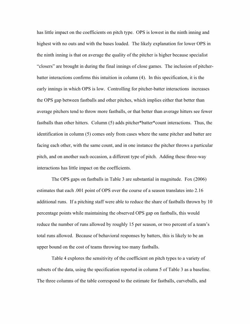
has little impact on the coefficients on pitch type. OPS is lowest in the ninth inning and

highest with no outs and with the bases loaded. The likely explanation for lower OPS in

the ninth inning is that on average the quality of the pitcher is higher because specialist

“closers” are brought in during the final innings of close games. The inclusion of pitcher-

batter interactions confirms this intuition in column (4). In this specification, it is the

early innings in which OPS is low. Controlling for pitcher-batter interactions increases

the OPS gap between fastballs and other pitches, which implies either that better than

average pitchers tend to throw more fastballs, or that better than average hitters see fewer

fastballs than other hitters. Column (5) adds pitcher*batter*count interactions. Thus, the

identification in column (5) comes only from cases where the same pitcher and batter are

facing each other, with the same count, and in one instance the pitcher throws a particular

pitch, and on another such occasion, a different type of pitch. Adding these three-way

interactions has little impact on the coefficients.

The OPS gaps on fastballs in Table 3 are substantial in magnitude. Fox (2006)

estimates that each .001 point of OPS over the course of a season translates into 2.16

additional runs. If a pitching staff were able to reduce the share of fastballs thrown by 10

percentage points while maintaining the observed OPS gap on fastballs, this would

reduce the number of runs allowed by roughly 15 per season, or two percent of a team’s

total runs allowed. Because of behavioral responses by batters, this is likely to be an

upper bound on the cost of teams throwing too many fastballs.

Table 4 explores the sensitivity of the coefficient on pitch types to a variety of

subsets of the data, using the specification reported in column 5 of Table 3 as a baseline.

The three columns of the table correspond to the estimate for fastballs, curveballs, and

sliders respectively, in all cases relative to the omitted category, which is changeups.

Each row of the table represents estimates from one regression; only the coefficients on

the pitch type variables are presented in the table.

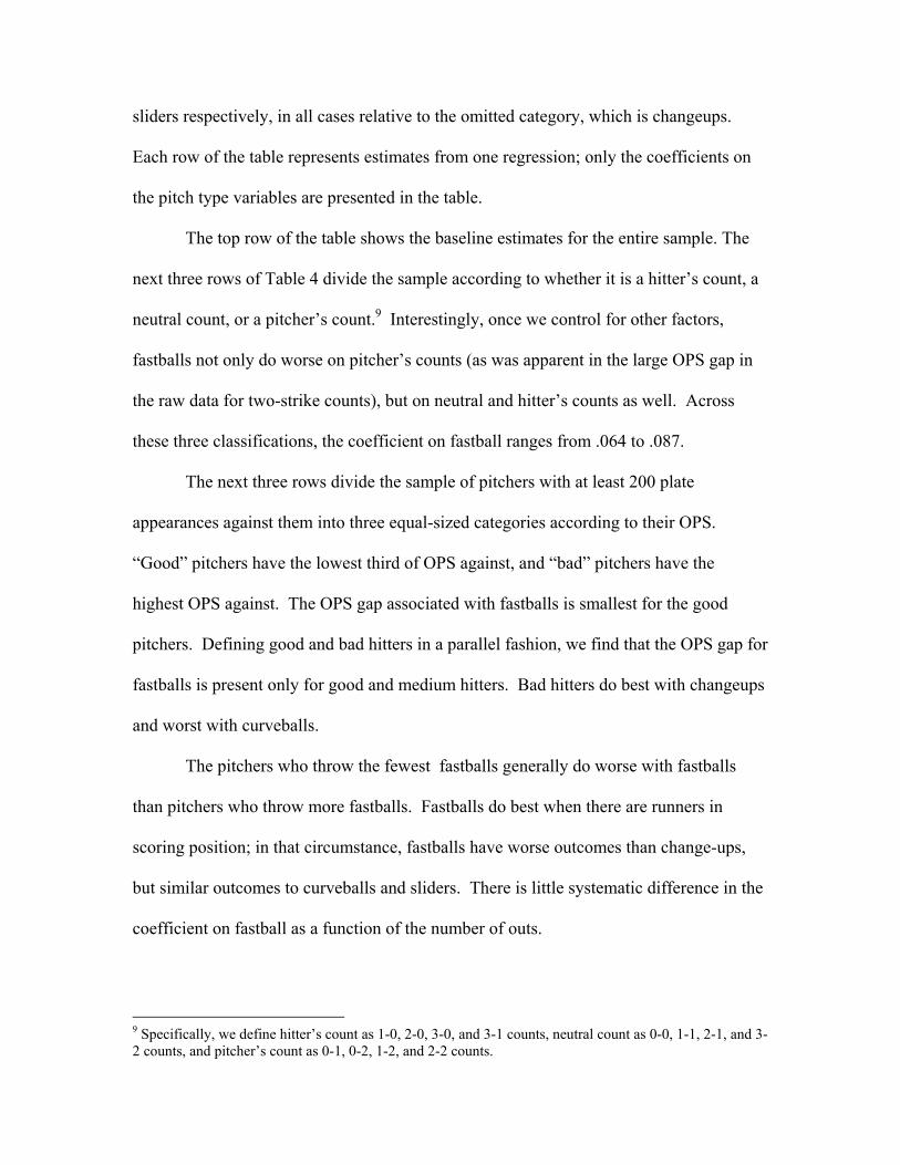
The top row of the table shows the baseline estimates for the entire sample. The

next three rows of Table 4 divide the sample according to whether it is a hitter’s count, a

neutral count, or a pitcher’s count.9 Interestingly, once we control for other factors,

fastballs not only do worse on pitcher’s counts (as was apparent in the large OPS gap in

the raw data for two-strike counts), but on neutral and hitter’s counts as well. Across

these three classifications, the coefficient on fastball ranges from .064 to .087.

The next three rows divide the sample of pitchers with at least 200 plate

appearances against them into three equal-sized categories according to their OPS.

“Good” pitchers have the lowest third of OPS against, and “bad” pitchers have the

highest OPS against. The OPS gap associated with fastballs is smallest for the good

pitchers. Defining good and bad hitters in a parallel fashion, we find that the OPS gap for

fastballs is present only for good and medium hitters. Bad hitters do best with changeups

and worst with curveballs.

The pitchers who throw the fewest fastballs generally do worse with fastballs

than pitchers who throw more fastballs. Fastballs do best when there are runners in

scoring position; in that circumstance, fastballs have worse outcomes than change-ups,

but similar outcomes to curveballs and sliders. There is little systematic difference in the

coefficient on fastball as a function of the number of outs.

9 Specifically, we define hitter’s count as 1-0, 2-0, 3-0, and 3-1 counts, neutral count as 0-0, 1-1, 2-1, and 3-2 counts, and pitcher’s count as 0-1, 0-2, 1-2, and 2-2 counts.

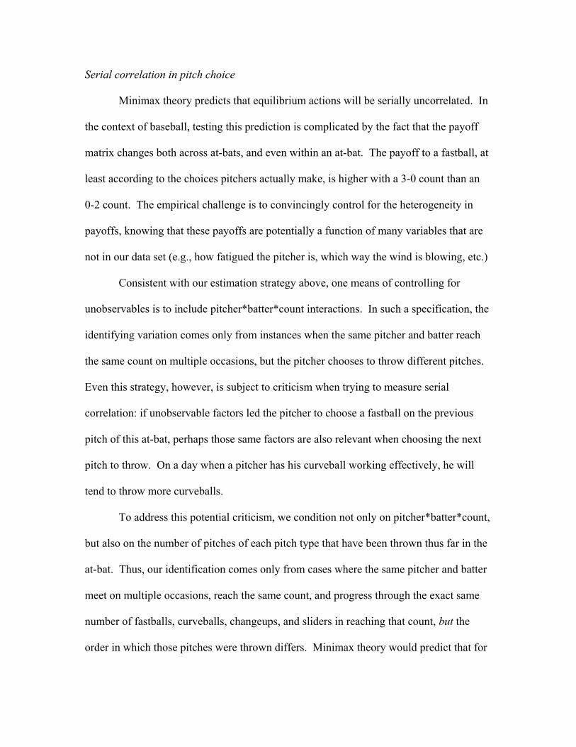
Serial correlation in pitch choice

Minimax theory predicts that equilibrium actions will be serially uncorrelated. In

the context of baseball, testing this prediction is complicated by the fact that the payoff

matrix changes both across at-bats, and even within an at-bat. The payoff to a fastball, at

least according to the choices pitchers actually make, is higher with a 3-0 count than an

0-2 count. The empirical challenge is to convincingly control for the heterogeneity in

payoffs, knowing that these payoffs are potentially a function of many variables that are

not in our data set (e.g., how fatigued the pitcher is, which way the wind is blowing, etc.)

Consistent with our estimation strategy above, one means of controlling for

unobservables is to include pitcher*batter*count interactions. In such a specification, the

identifying variation comes only from instances when the same pitcher and batter reach

the same count on multiple occasions, but the pitcher chooses to throw different pitches.

Even this strategy, however, is subject to criticism when trying to measure serial

correlation: if unobservable factors led the pitcher to choose a fastball on the previous

pitch of this at-bat, perhaps those same factors are also relevant when choosing the next

pitch to throw. On a day when a pitcher has his curveball working effectively, he will

tend to throw more curveballs.

To address this potential criticism, we condition not only on pitcher*batter*count,

but also on the number of pitches of each pitch type that have been thrown thus far in the

at-bat. Thus, our identification comes only from cases where the same pitcher and batter

meet on multiple occasions, reach the same count, and progress through the exact same

number of fastballs, curveballs, changeups, and sliders in reaching that count, but the

order in which those pitches were thrown differs. Minimax theory would predict that for

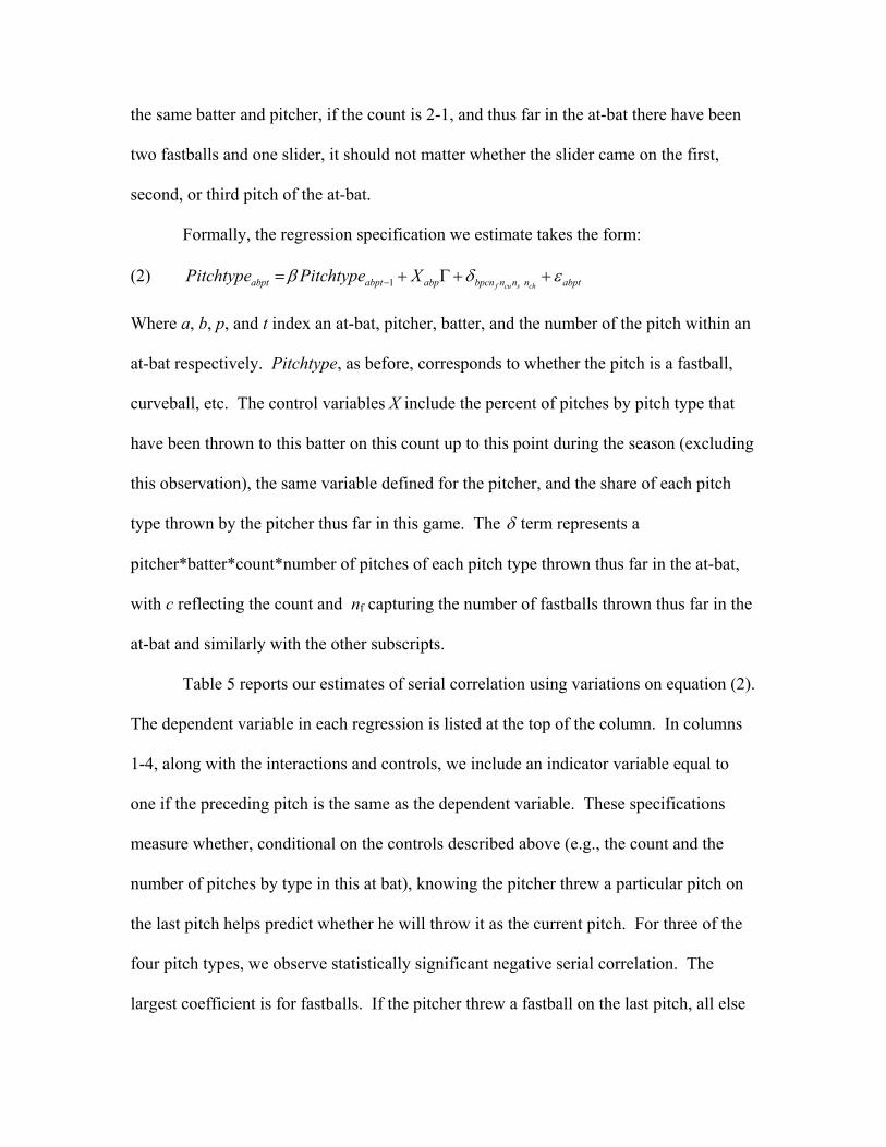
the same batter and pitcher, if the count is 2-1, and thus far in the at-bat there have been

two fastballs and one slider, it should not matter whether the slider came on the first,

second, or third pitch of the at-bat.

Formally, the regression specification we estimate takes the form:

(2) 1 f cu s chabpt abpt abp bpcn n n n abptPitchtype Pitchtype Xβ δ ε−= + Γ + +

Where a, b, p, and t index an at-bat, pitcher, batter, and the number of the pitch within an

at-bat respectively. Pitchtype, as before, corresponds to whether the pitch is a fastball,

curveball, etc. The control variables X include the percent of pitches by pitch type that

have been thrown to this batter on this count up to this point during the season (excluding

this observation), the same variable defined for the pitcher, and the share of each pitch

type thrown by the pitcher thus far in this game. The δ term represents a

pitcher*batter*count*number of pitches of each pitch type thrown thus far in the at-bat,

with c reflecting the count and nf capturing the number of fastballs thrown thus far in the

at-bat and similarly with the other subscripts.

Table 5 reports our estimates of serial correlation using variations on equation (2).

The dependent variable in each regression is listed at the top of the column. In columns

1-4, along with the interactions and controls, we include an indicator variable equal to

one if the preceding pitch is the same as the dependent variable. These specifications

measure whether, conditional on the controls described above (e.g., the count and the

number of pitches by type in this at bat), knowing the pitcher threw a particular pitch on

the last pitch helps predict whether he will throw it as the current pitch. For three of the

four pitch types, we observe statistically significant negative serial correlation. The

largest coefficient is for fastballs. If the pitcher threw a fastball on the last pitch, all else

equal, it lowers the likelihood this pitch will be a fastball by 4.1 percentage points. In

relative terms, the negative serial correlation for sliders is greater, since sliders represent

only about 10 percent of all pitches. If the last pitch was a slider, the likelihood that this

current pitch is a slider falls by two percentage points, or twenty percent. The negative

serial correlation is roughly half as large for curveballs, and not present for changeups.

Columns 5-8 of Table 5 add the indicators for once-lagged values of each pitch

type, which allows us to learn not just whether pitchers repeat the same pitch more or less

than would be expected, but also whether other transitional sequences from pitch to pitch

appear more or less frequently than predicted by theory. In each of these columns, one of

the lagged pitch types is omitted, and all results are relative to that omitted category. The

results that emerge in columns 5-8 demonstrate that there is greater nuance associated

with the ordering of pitches than simply the negative serial correlation observed in the

first four columns. For instance, in column 5, not only is it the case that fastballs follow

fastballs less than would be expected, but also, fastballs are more likely to occur after

changeups than after other non-fastballs. In contrast, curveballs are least likely to follow

changeups (and vice versa), and curveballs are most likely to follow fastballs.

Changeups are more likely to occur if the last pitch was a changeup than it was another

non-fastball.

Calibrating the value to a team’s batters of exploiting these correlation patterns

requires making assumptions as to how valuable it is to a major league hitter to know

what type of pitch is coming. Executives of Major League Baseball teams with whom we

spoke estimated that there would be a .150 gap in OPS between a batter who knew for a

certain a fastball was coming versus that same batter who mistakenly thought that there

was a 100 percent change the next pitch would not be a fastball, but in fact was surprised

and faced a fastball. If one makes the further assumption that the OPS gap is linear in a

hitter’s expectations about what type of pitch will be coming, then knowing that a fastball

is 4.1 percentage points less likely if the last pitch was a fastball (and conversely more

likely if the last pitch was not a fast ball) is worth roughly .006 OPS points to a batter.

Thus, the potential benefit from exploiting the patterns of serial correlation is the same

magnitude as identified earlier from pitchers throwing too many fastballs – about 10-15

runs per year.

Section II: An analysis of play selection in the National Football League

Our data on play choice in the National Football League was compiled by

STATS, Inc. STATS, Inc. maintains a network of reporters tracking every snap in detail

to provide exclusive information from their proprietary database to the NFL and other

clients. The data set includes extensive information for each play in the NFL over the

period 2001-2005: date of game, offensive team, defensive team, general game

description (e.g., stadium, weather, etc.), current game situation (quarter, location on

field, down, yards to go, etc.), offensive formation, the type of play (run, pass, punt, field

goal, etc.), and the outcome of the play (e.g., yards gained).

As was the case with baseball, there are many dimensions on which play types

vary: run or pass, direction, distance, movement of players, etc. We limit our study to

just one dimension: the choice of whether to call a running play or a passing play.

Our raw data covers every play from regular season NFL games over five full

seasons: 2001-2005. We exclude fourth down plays, as well as all plays that occur in the

last two minutes of the half, during overtime, or when a team kneels down to run out the

clock. Because of difficulties in our data of identifying whether the team’s intention was

to run or to pass on plays where the quarterback runs, and on penalties called before a

play unfolds (e.g., false start), these plays are also excluded. After these exclusions, we

have 127,885 total plays.

Unlike baseball, where there are well-established summary metrics for

evaluating the success of an at bat (e.g. OPS), there is no parallel statistic in football.

Consequently, we construct our own measure of success for a play in football as follows.

First, we estimate the value to a team of having possession of the ball as a function of

distance from the end zone, what down it is, and yards to achieve a first down, using a

regression taking the form

(3) (down, yards to first down, distance to goal)Y f=

where the outcome variable Y is the change in the game score between the current time

and the end of the half. We allow for a flexible function form with respect to the right-

hand-side variables, including fully interacted quintics of each of the variables. The

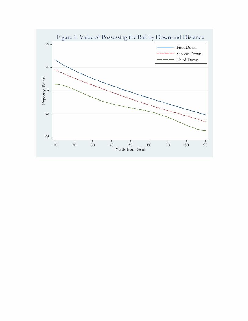
values generated from equation (3) appear sensible. For instance, the three lines in

Figure 1 show the estimated value to a team of having the ball first down and ten yards to

go, second down and ten yards to go, and third down and ten yards to go respectively as a

function of the distance to the end zone. 10 If a team has the ball first and ten at the

opponent’s ten yard line, that team will expect to gain more than four points relative to

the other team by the end of the half. The value of having the ball first and ten declines 10 One other measure of performance in NFL football is Net Expected Scoring (NES), developed by Citizen Sports Network. NES is not as flexible as our success metric, but is highly correlated (ρ=. 0.8583) with our success metric.

nearly linearly with field position; having the ball first and ten on one’s own ten yard line

is associated with essentially no expected change in the half-time score. Having the ball

second and ten costs a team about one-half a point relative to having the ball first and ten

from the same field position. Moving from second and ten to third and ten is even more

costly for a team.

To compute how successful a particular play is, we calculate the change in

expected points scored before and after the play (e.g., looking at Figure 1, if a team gains

20 yards when it is first and ten from its own 20 yard line, expected points scored jump

by roughly one) and subtract the average change in expected points for all plays in the

data set that began at the same down, distance, and yards to the goal.11 The resulting

statistic, which we call our “success metric,” is mean zero. The success metric tells us, in

units of expected points scored, how much this play exceeds or underperforms the

average play run on this down, distance, and yards to goal.

In addition to this constructed measure of success, we also report results for more

traditional, but highly imperfect outcome measures: yards gained,12 whether a first down

is made, whether points are scored, and whether a turnover occurs.

Table 6 reports summary statistics for the football data set. Column 1 shows

outcomes for all plays; columns 2 and 3 divide the sample into running plays and passing

plays respectively. Column 4 reports the t-statistic of the comparison of means between

running and passing plays. Overall, runs represent 44 percent of the combined passes and

runs. For all plays our success metric, by definition, has a mean value of zero, since it is

11 When the play results in points being scored, those points are included in our calculation of the metric. 12 We adjusted yards gained per play to capture certain circumstances: penalty yardage for penalties occurring within plays were incorporated, touchdowns within 10 yards of end zone were credited with a full 10 yards gained, and interceptions were adjusted to -45 yards gained.

defined as the deviation from the expected outcome on a play. Note, however,

comparing the top row of columns 2 and 3, that passing plays systematically outperform

running plays. The mean gap between the two types of plays is roughly .066, implying

that on average, a passing play generates .066 more points than a run. This difference in

means is highly statistically significant. Consistent with this result, passes on average

yield an extra .55 yards gained, and are nine percentage points more likely to yield a first

down. Passes do, however, produce more turnovers, and thus have higher variance. Runs

result in scoring plays 2.8 percent of the time; passes lead to scores with a 3.8 percent

probability.

To further analyze the difference across runs and passes, we estimate regressions

of the form :

(4) pijijpijpijpij XPassOutcome ελβα ++Γ++=

where p, i, and j index a particular play, offensive team, and defending team respectively.

Outcome is our measure of success for an offensive play. Pass is an indicator variable

equal to one if the team calls a passing play, and zero if the play is designed to be a run.

X is a vector of controls, such as the score differential at the time of the play, whether the

game is played on grass, whether the offensive team is the home team, the year of the

game, etc. In some specifications, we also add team-fixed effects for the offense and the

defense, or interactions between the offensive and defensive teams.

The results from estimating equation (4) are presented in Table 7. The four

columns represent four different specifications, with the number of controls increasing

moving from left to right in the table. The first column, which includes no covariates,

confirms the raw difference in means between passing and running; a pass generates an

additional .066 points in expectation. Column 2 adds controls, but does not include team-

fixed effects. The relative value of a pass increases to .083 points in this specification.

This specification also highlights the sizable home field advantage in the NFL: an

offensive play run by the home team generate an extra .041 points, or roughly half the

difference between a pass and a run. Offenses perform slightly worse in the cold. The

playing surface does not have a large impact on the offense’s effectiveness.

Column 3 adds fixed-effects for the offensive and defensive teams. These fixed

effects will absorb any systematic differences across teams in offensive and defensive

prowess. The relative value of a pass decreases slightly to .077 points in this

specification. The last column of the table includes interaction effects for the offensive

and defensive teams. The relative value of a pass is essentially unchanged at .075 points.

Table 8 examines the sensitivity of the results of running versus passing to a

variety of subsets of the data, as well as reporting results for an expanded set of outcome

measures (yards gained, achieving a first down on the play, turnovers, and whether a

touchdown is scored on the play). The columns of the table correspond to different

outcome measures, e.g. our constructed success metric, yards gained, etc. Each row of

the table represents a different subset of the data. In all cases, we include team-fixed

effects and controls mirroring those in column 4 of Table 7. Only the coefficient on the

pass indicator variable is reported in the table.

Focusing first on the column 1 of Table 8, the top row of the table reports our

baseline specification. Thus, the entry in the top row in column 1 matches the coefficient

we report in Table 6, column 4: a .075 gap between passes and runs on our success

metric. Consistent with this result, passes do better on yards gained, first downs made,

and scoring, but also lead to more turnovers. Moving down through the table, passes

outperform runs in all quarters of the game, but by a greater margin in the first half than

the second half of the game. The benefits of passing accrue equally to home teams and

visitors. The best offenses exhibit the greatest gap between passes and runs; for the worst

offenses the differential is not statistically significant. Teams that pass the most have

slightly smaller edges when passing than other teams.

The results in Tables 7 and 8 demonstrate that the expected outcome of a pass

systematically exceeds that of a run – a result that is inconsistent with Minimax theory.13

According to the theory, defenses should adjust to better defend the pass. Absent that

adjustment, offenses should be passing more often. The magnitude of the deviations in

payoffs that are observed are substantial. The typical offense runs about 60 plays a game,

56 percent of which are passes. If the offense could increase its share of passes to 70

percent without inducing an offsetting response on the part of the defense, it would

generate an additional 0.63 points per game in expectation (8.4 additional passes*0.075

expected points), or an extra ten points over the course of a season, or roughly 3 percent

of a team’s total scoring. Because defenses are likely to respond, that estimate is likely

an upper bound on how much an offense could gain by exploiting the deviations from

minimax play that are present in the data.

13 Alamar (2006) shows passing plays as having an outcome advantage of nearly 1.8 yards per play (adjusted yards) for the 2005 NFL season. However, the source of that data -- http://www.pro-football-reference.com/years/2005/ -- shows a difference of 0.5 yards when considering both sacks and interceptions as passing plays (“Adjusted Net Yards gained per pass attempt”), which is consistent with our findings.

Serial correlation in NFL play calling

To assess whether there is serial correlation in the choice of runs versus passes on

the part of NFL offenses, we run regressions of the form

(5) pijpijijppij XPassPass εβα +Γ++= −1

where Pass is an indicator for whether the play called was intended to be a pass. The

coefficient β captures the degree of serial correlation in play calling. Included in the

vector of controls are the same set of covariates in the earlier football analysis, along with

three additional variables: the percentage of time that the offensive team passed over the

course of the entire season, the percentage of time that the defensive team was passed

against over the course of the entire season, and the share of passes by the offense in this

game, up until the time this play is called. Because we control for down and distance in

these regressions, as well as an offense’s overall tendencies towards passing versus

running, our identification comes from a comparison of, for example, whether on 2nd

down and 10, a pass is more likely if the previous play was a run that went for no gain, or

the previous play was an incomplete pass. Minimax play predicts no serial correlation,

implying a zero coefficient on whether or not the last play was a pass.

The basic estimation results corresponding to equation 5 are presented in column

1 of Table 9.14 Offensive play calling reveals substantial negative serial correlation, with

a coefficient of -.100 (se=.003). In other words, conditional on other factors, a team is

14 The number of observations in Table 9 is smaller than in the earlier analysis for two reasons. First, the first play of each drive is not included in the serial correlation analysis. Second, plays for which the preceding play could not be cataloged as a run or a pass (e.g. because of a penalty or a quarterback run) are also excluded.

almost 10 percentage points less likely to pass on this current play if they passed on the

previous play.

To further explore the question of serial correlation, we divide the sample into

thirds according to how successful the previous play was, with success defined by our

constructed success metric The results for these three subsets of the data (i.e. previous

play was in the bottom-third/middle-third/upper-third success-wise) are shown in

columns 2 through 4 of Table 9. Negative serial correlation is most pronounced when the

preceding play was unsuccessful. Experiencing a poor result on the last play increases

the likelihood the team will switch from a run to a pass or vice-versa by 14.5 percentage

points. In contrast, when the last play is in the upper-third of successful outcomes, the

tendency to switch away from that play type is greatly mitigated (serial correlation

coefficient of only -.025).

These coefficients imply the opportunity for non-trivial gains for teams that

successfully exploit serial correlation on the part of opposing offenses. Assume, for

instance, that if a defense knew with 100 percent certainty whether a play would be a run

or a pass, it could cut the average yardage gained in half by adjusting defensive personnel

or positioning. Assume, as well, that if the defense was 100 percent certain a pass was

coming, but instead the offense ran the ball, the expected yardage gained would be 50

percent greater than the average, and similarly if the defense expected a run and the

offense passed.15 Finally, let us assume that the value of knowing what play is coming is

linear in the probabilities, i.e. going from 50 percent likelihood of a run to 60 percent

likelihood yields one-tenth of the benefit of going from zero percent to 100 percent. Take

15 Based on discussions with NFL teams, these assumptions are likely to be conservative, understating the potential value to defenses of exploiting serial correlated offensive play.

the case where absent serial correlation, a defense expects an equal mix of runs and

passes, with each type of play gaining 4.5 yards on average. With serial correlation,

however, the true mix of plays after a pass will be roughly 60 percent runs and 40 percent

passes. Under the assumptions above, if the defense adjusts to this information, the

average running play will yield 3.6 yards and the average passing play 5.4 yards, yielding

an overall average gain for the offense of 4.32 yards –.18 yards less than if the defense

ignores the serial correlation. There are roughly 60 offensive play calls per game that are

preceded by another offensive play. If the average reduction in yards gained per play is

.18 yards, then this amounts to an overall reduction of 10.8 yards per game, which

translates into roughly 1 point per game. One point per game is worth approximately a

half victory per year – considerable given the NFL regular season includes just sixteen

games.16 The potential benefit from exploiting the patterns of serial correlation in

football is slightly larger than the benefit from calling fewer running plays analyzed

earlier.

16 We base this calculation on the change in expected winning percentage by scoring 16 additional season points as estimated by the Pythagorean Winning Percentage [expected winning percentage = (points scored^2.64)/(points scored^2.64 + points allowed^2.64)]. Taking an average NFL team with 350 season points scored and 350 points allowed, increasing their points scored to 366 increases their expected winning percentage from .500 to .529.

Section IV: Conclusion

In this paper, we utilize two enormous data sets generated by professionals in a

high stakes environment to provide the most powerful test to date of minimax behavior in

a natural setting. In contrast to most prior studies using field data, we find substantial

deviations from minimax behavior, both with respect to equalizing payoffs and serially

correlated actions. These deviations are not enormous in magnitude – meaning that they

might plausibly not have been detected in the smaller data sets that have been available in

most prior field research on the topic – but are large enough that a team that successfully

exploited these patterns could add one or two season wins and millions of dollars in

associated revenue.

Our findings reinforce the results of Romer (2006), Levitt (2006), and Pope and

Schweitzer (2009) in demonstrating that high stakes alone are not sufficient to ensure that

optimal decision-making will ensue, even among professionals operating in their natural

environments.

-20

24

6E

xpec

ted

Poin

ts

10 20 30 40 50 60 70 80 90Yards from Goal

First DownSecond DownThird Down

Figure 1: Value of Possessing the Ball by Down and Distance

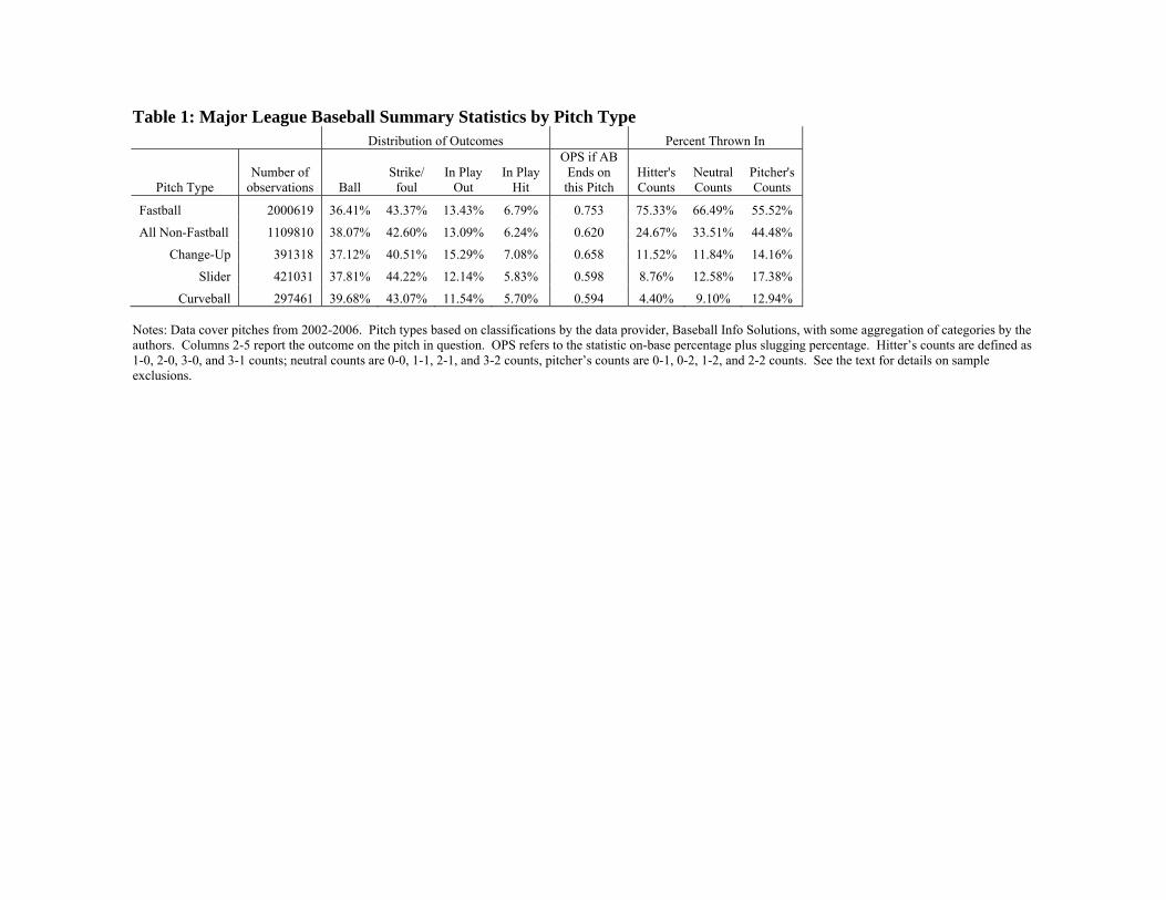
Table 1: Major League Baseball Summary Statistics by Pitch Type Distribution of Outcomes Percent Thrown In

Pitch Type Number of

observations Ball Strike/

foul In Play

Out In Play

Hit

OPS if AB Ends on

this Pitch Hitter's Counts

Neutral Counts

Pitcher's Counts

Fastball 2000619 36.41% 43.37% 13.43% 6.79% 0.753 75.33% 66.49% 55.52%

All Non-Fastball 1109810 38.07% 42.60% 13.09% 6.24% 0.620 24.67% 33.51% 44.48%

Change-Up 391318 37.12% 40.51% 15.29% 7.08% 0.658 11.52% 11.84% 14.16%

Slider 421031 37.81% 44.22% 12.14% 5.83% 0.598 8.76% 12.58% 17.38%

Curveball 297461 39.68% 43.07% 11.54% 5.70% 0.594 4.40% 9.10% 12.94% Notes: Data cover pitches from 2002-2006. Pitch types based on classifications by the data provider, Baseball Info Solutions, with some aggregation of categories by the authors. Columns 2-5 report the outcome on the pitch in question. OPS refers to the statistic on-base percentage plus slugging percentage. Hitter’s counts are defined as 1-0, 2-0, 3-0, and 3-1 counts; neutral counts are 0-0, 1-1, 2-1, and 3-2 counts, pitcher’s counts are 0-1, 0-2, 1-2, and 2-2 counts. See the text for details on sample exclusions.

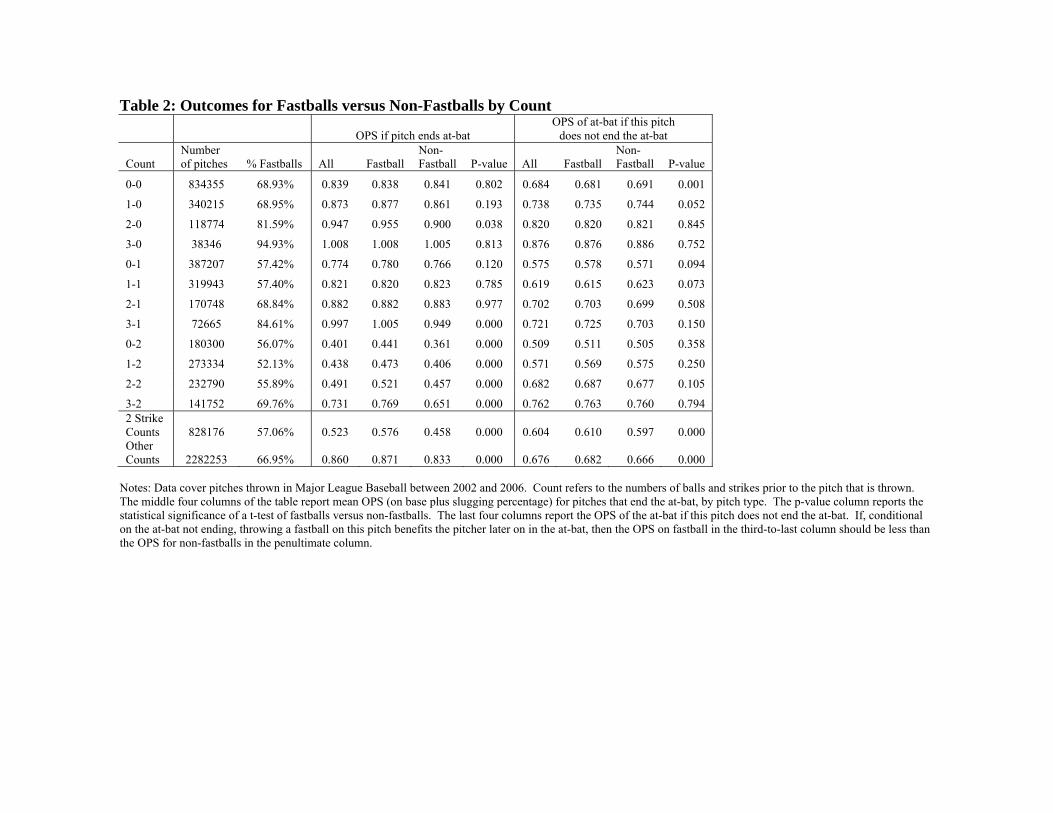
Table 2: Outcomes for Fastballs versus Non-Fastballs by Count

OPS if pitch ends at-bat OPS of at-bat if this pitch

does not end the at-bat

Count Number of pitches % Fastballs All Fastball

Non- Fastball P-value All Fastball

Non-Fastball P-value

0-0 834355 68.93% 0.839 0.838 0.841 0.802 0.684 0.681 0.691 0.001

1-0 340215 68.95% 0.873 0.877 0.861 0.193 0.738 0.735 0.744 0.052

2-0 118774 81.59% 0.947 0.955 0.900 0.038 0.820 0.820 0.821 0.845

3-0 38346 94.93% 1.008 1.008 1.005 0.813 0.876 0.876 0.886 0.752

0-1 387207 57.42% 0.774 0.780 0.766 0.120 0.575 0.578 0.571 0.094

1-1 319943 57.40% 0.821 0.820 0.823 0.785 0.619 0.615 0.623 0.073

2-1 170748 68.84% 0.882 0.882 0.883 0.977 0.702 0.703 0.699 0.508

3-1 72665 84.61% 0.997 1.005 0.949 0.000 0.721 0.725 0.703 0.150

0-2 180300 56.07% 0.401 0.441 0.361 0.000 0.509 0.511 0.505 0.358

1-2 273334 52.13% 0.438 0.473 0.406 0.000 0.571 0.569 0.575 0.250

2-2 232790 55.89% 0.491 0.521 0.457 0.000 0.682 0.687 0.677 0.105

3-2 141752 69.76% 0.731 0.769 0.651 0.000 0.762 0.763 0.760 0.794 2 Strike Counts 828176 57.06% 0.523 0.576 0.458 0.000 0.604 0.610 0.597 0.000 Other Counts 2282253 66.95% 0.860 0.871 0.833 0.000 0.676 0.682 0.666 0.000

Notes: Data cover pitches thrown in Major League Baseball between 2002 and 2006. Count refers to the numbers of balls and strikes prior to the pitch that is thrown. The middle four columns of the table report mean OPS (on base plus slugging percentage) for pitches that end the at-bat, by pitch type. The p-value column reports the statistical significance of a t-test of fastballs versus non-fastballs. The last four columns report the OPS of the at-bat if this pitch does not end the at-bat. If, conditional on the at-bat not ending, throwing a fastball on this pitch benefits the pitcher later on in the at-bat, then the OPS on fastball in the third-to-last column should be less than the OPS for non-fastballs in the penultimate column.

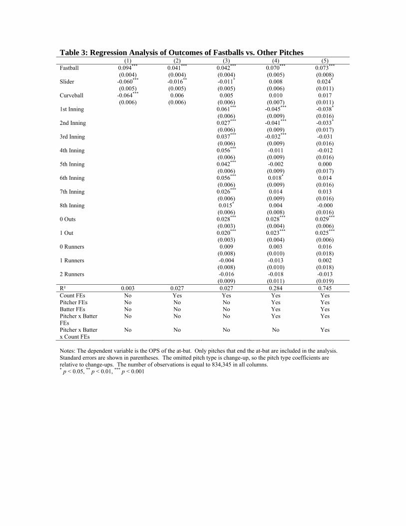
Table 3: Regression Analysis of Outcomes of Fastballs vs. Other Pitches (1) (2) (3) (4) (5) Fastball 0.094*** 0.041*** 0.042*** 0.070*** 0.073*** (0.004) (0.004) (0.004) (0.005) (0.008) Slider -0.060*** -0.016** -0.011* 0.008 0.024* (0.005) (0.005) (0.005) (0.006) (0.011) Curveball -0.064*** 0.006 0.005 0.010 0.017 (0.006) (0.006) (0.006) (0.007) (0.011) 1st Inning 0.061*** -0.045*** -0.038* (0.006) (0.009) (0.016) 2nd Inning 0.027*** -0.041*** -0.033* (0.006) (0.009) (0.017) 3rd Inning 0.037*** -0.032*** -0.031 (0.006) (0.009) (0.016) 4th Inning 0.056*** -0.011 -0.012 (0.006) (0.009) (0.016) 5th Inning 0.042*** -0.002 0.000 (0.006) (0.009) (0.017) 6th Inning 0.056*** 0.018* 0.014 (0.006) (0.009) (0.016) 7th Inning 0.026*** 0.014 0.013 (0.006) (0.009) (0.016) 8th Inning 0.015* 0.004 -0.000 (0.006) (0.008) (0.016) 0 Outs 0.028*** 0.028*** 0.029*** (0.003) (0.004) (0.006) 1 Out 0.020*** 0.023*** 0.025*** (0.003) (0.004) (0.006) 0 Runners 0.009 0.003 0.016 (0.008) (0.010) (0.018) 1 Runners -0.004 -0.013 0.002 (0.008) (0.010) (0.018) 2 Runners -0.016 -0.018 -0.013 (0.009) (0.011) (0.019) R² 0.003 0.027 0.027 0.284 0.745 Count FEs No Yes Yes Yes Yes Pitcher FEs No No No Yes Yes Batter FEs No No No Yes Yes Pitcher x Batter FEs

No No No Yes Yes

Pitcher x Batter x Count FEs

No No No No Yes

Notes: The dependent variable is the OPS of the at-bat. Only pitches that end the at-bat are included in the analysis. Standard errors are shown in parentheses. The omitted pitch type is change-up, so the pitch type coefficients are relative to change-ups. The number of observations is equal to 834,345 in all columns. * p < 0.05, ** p < 0.01, *** p < 0.001

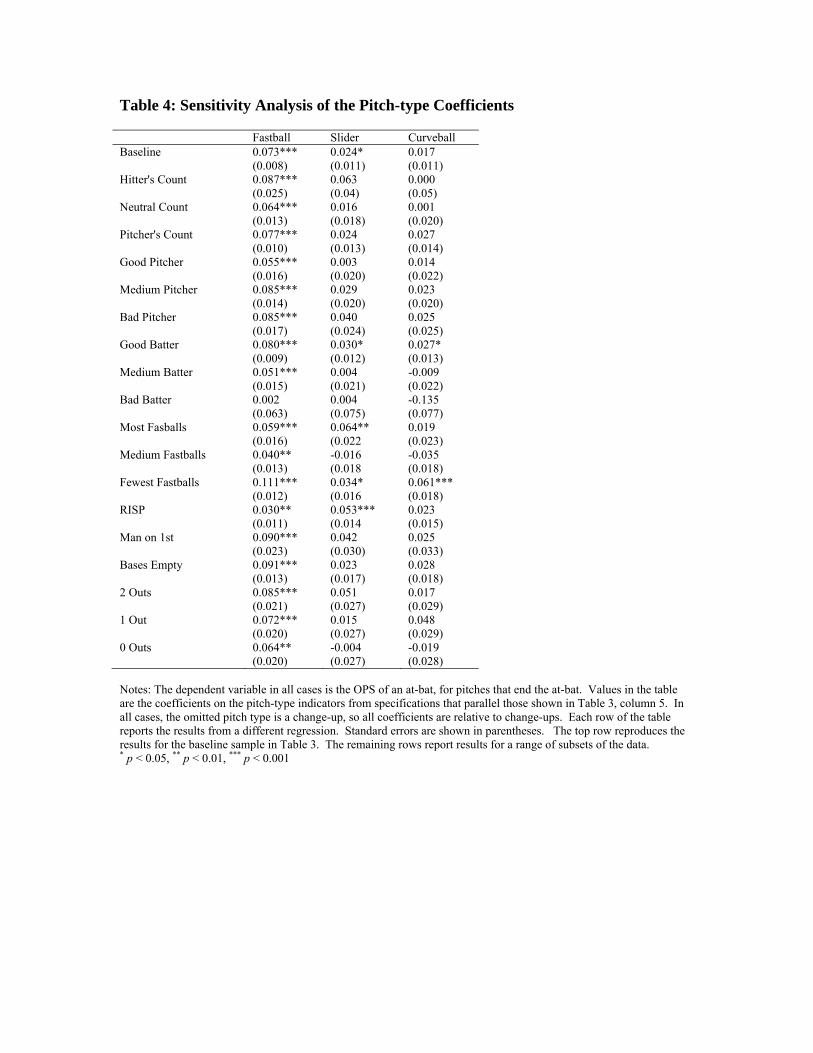
Table 4: Sensitivity Analysis of the Pitch-type Coefficients

Fastball Slider Curveball Baseline 0.073*** 0.024* 0.017 (0.008) (0.011) (0.011) Hitter's Count 0.087*** 0.063 0.000 (0.025) (0.04) (0.05) Neutral Count 0.064*** 0.016 0.001 (0.013) (0.018) (0.020) Pitcher's Count 0.077*** 0.024 0.027 (0.010) (0.013) (0.014) Good Pitcher 0.055*** 0.003 0.014 (0.016) (0.020) (0.022) Medium Pitcher 0.085*** 0.029 0.023 (0.014) (0.020) (0.020) Bad Pitcher 0.085*** 0.040 0.025 (0.017) (0.024) (0.025) Good Batter 0.080*** 0.030* 0.027* (0.009) (0.012) (0.013) Medium Batter 0.051*** 0.004 -0.009 (0.015) (0.021) (0.022) Bad Batter 0.002 0.004 -0.135 (0.063) (0.075) (0.077) Most Fasballs 0.059*** 0.064** 0.019 (0.016) (0.022 (0.023) Medium Fastballs 0.040** -0.016 -0.035 (0.013) (0.018 (0.018) Fewest Fastballs 0.111*** 0.034* 0.061*** (0.012) (0.016 (0.018) RISP 0.030** 0.053*** 0.023 (0.011) (0.014 (0.015) Man on 1st 0.090*** 0.042 0.025 (0.023) (0.030) (0.033) Bases Empty 0.091*** 0.023 0.028 (0.013) (0.017) (0.018) 2 Outs 0.085*** 0.051 0.017 (0.021) (0.027) (0.029) 1 Out 0.072*** 0.015 0.048 (0.020) (0.027) (0.029) 0 Outs 0.064** -0.004 -0.019 (0.020) (0.027) (0.028) Notes: The dependent variable in all cases is the OPS of an at-bat, for pitches that end the at-bat. Values in the table are the coefficients on the pitch-type indicators from specifications that parallel those shown in Table 3, column 5. In all cases, the omitted pitch type is a change-up, so all coefficients are relative to change-ups. Each row of the table reports the results from a different regression. Standard errors are shown in parentheses. The top row reproduces the results for the baseline sample in Table 3. The remaining rows report results for a range of subsets of the data. * p < 0.05, ** p < 0.01, *** p < 0.001

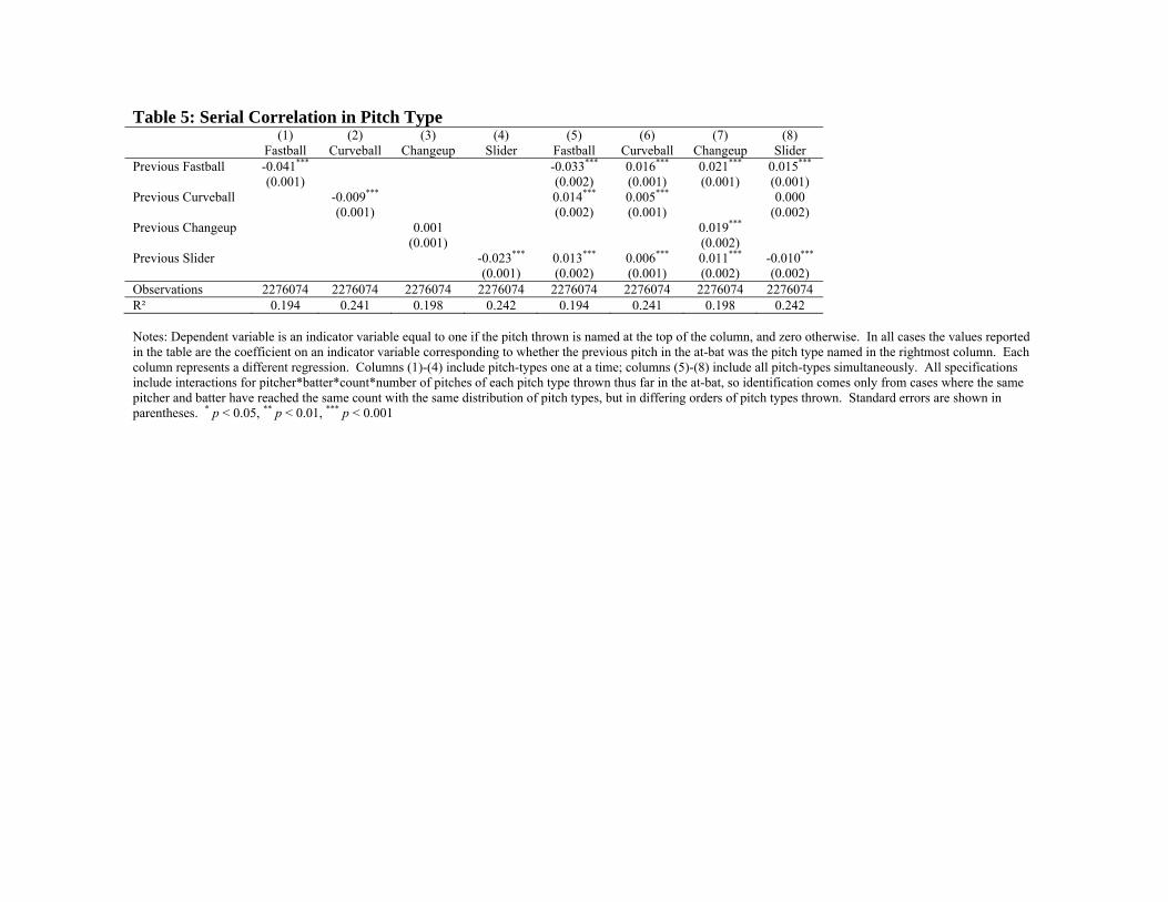
Table 5: Serial Correlation in Pitch Type (1) (2) (3) (4) (5) (6) (7) (8) Fastball Curveball Changeup Slider Fastball Curveball Changeup Slider Previous Fastball -0.041*** -0.033*** 0.016*** 0.021*** 0.015*** (0.001) (0.002) (0.001) (0.001) (0.001) Previous Curveball -0.009*** 0.014*** 0.005*** 0.000 (0.001) (0.002) (0.001) (0.002) Previous Changeup 0.001 0.019*** (0.001) (0.002) Previous Slider -0.023*** 0.013*** 0.006*** 0.011*** -0.010*** (0.001) (0.002) (0.001) (0.002) (0.002) Observations 2276074 2276074 2276074 2276074 2276074 2276074 2276074 2276074 R² 0.194 0.241 0.198 0.242 0.194 0.241 0.198 0.242 Notes: Dependent variable is an indicator variable equal to one if the pitch thrown is named at the top of the column, and zero otherwise. In all cases the values reported in the table are the coefficient on an indicator variable corresponding to whether the previous pitch in the at-bat was the pitch type named in the rightmost column. Each column represents a different regression. Columns (1)-(4) include pitch-types one at a time; columns (5)-(8) include all pitch-types simultaneously. All specifications include interactions for pitcher*batter*count*number of pitches of each pitch type thrown thus far in the at-bat, so identification comes only from cases where the same pitcher and batter have reached the same count with the same distribution of pitch types, but in differing orders of pitch types thrown. Standard errors are shown in parentheses. * p < 0.05, ** p < 0.01, *** p < 0.001

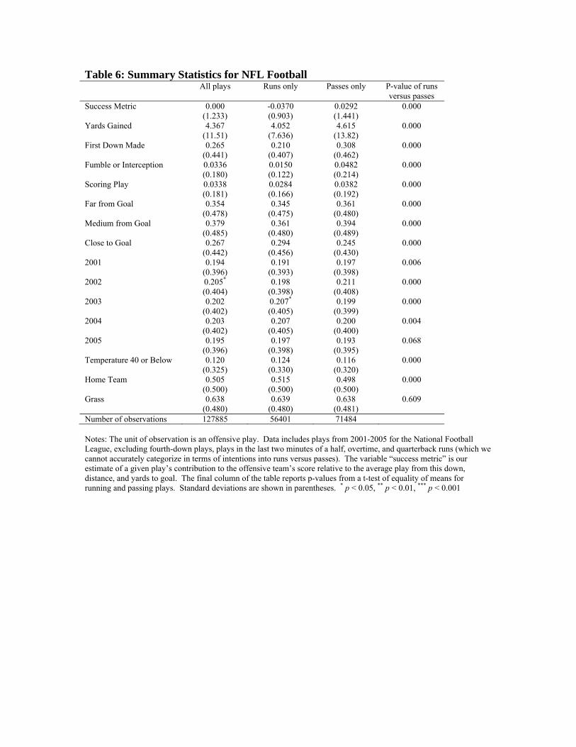
Table 6: Summary Statistics for NFL Football All plays Runs only Passes only P-value of runs

versus passes Success Metric 0.000 -0.0370 0.0292 0.000 (1.233) (0.903) (1.441) Yards Gained 4.367 4.052 4.615 0.000 (11.51) (7.636) (13.82) First Down Made 0.265 0.210 0.308 0.000 (0.441) (0.407) (0.462) Fumble or Interception 0.0336 0.0150 0.0482 0.000 (0.180) (0.122) (0.214) Scoring Play 0.0338 0.0284 0.0382 0.000 (0.181) (0.166) (0.192) Far from Goal 0.354 0.345 0.361 0.000 (0.478) (0.475) (0.480) Medium from Goal 0.379 0.361 0.394 0.000 (0.485) (0.480) (0.489) Close to Goal 0.267 0.294 0.245 0.000 (0.442) (0.456) (0.430) 2001 0.194 0.191 0.197 0.006 (0.396) (0.393) (0.398) 2002 0.205* 0.198 0.211 0.000 (0.404) (0.398) (0.408) 2003 0.202 0.207* 0.199 0.000 (0.402) (0.405) (0.399) 2004 0.203 0.207 0.200 0.004 (0.402) (0.405) (0.400) 2005 0.195 0.197 0.193 0.068 (0.396) (0.398) (0.395) Temperature 40 or Below 0.120 0.124 0.116 0.000 (0.325) (0.330) (0.320) Home Team 0.505 0.515 0.498 0.000 (0.500) (0.500) (0.500) Grass 0.638 0.639 0.638 0.609 (0.480) (0.480) (0.481) Number of observations 127885 56401 71484 Notes: The unit of observation is an offensive play. Data includes plays from 2001-2005 for the National Football League, excluding fourth-down plays, plays in the last two minutes of a half, overtime, and quarterback runs (which we cannot accurately categorize in terms of intentions into runs versus passes). The variable “success metric” is our estimate of a given play’s contribution to the offensive team’s score relative to the average play from this down, distance, and yards to goal. The final column of the table reports p-values from a t-test of equality of means for running and passing plays. Standard deviations are shown in parentheses. * p < 0.05, ** p < 0.01, *** p < 0.001

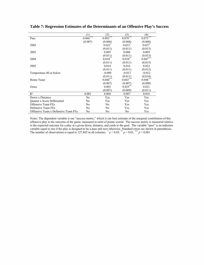
Table 7: Regression Estimates of the Determinants of an Offensive Play’s Success

(1) (2) (3) (4) Pass 0.066*** 0.083*** 0.078*** 0.075*** (0.007) (0.008) (0.008) (0.008) 2002 0.022* 0.023* 0.027* (0.011) (0.011) (0.013) 2003 0.005 0.006 0.005 (0.011) (0.011) (0.013) 2004 0.034** 0.034** 0.047*** (0.011) (0.011) (0.013) 2005 0.014 0.016 0.022 (0.011) (0.011) (0.012) Temperature 40 or below -0.009 -0.013 -0.012 (0.011) (0.011) (0.014) Home Team 0.040*** 0.043*** 0.048*** (0.007) (0.007) (0.008) Grass 0.003 0.025** 0.021 (0.007) (0.009) (0.011) R² 0.001 0.004 0.007 0.016 Down x Distance No Yes Yes Yes Quarter x Score Differential No Yes Yes Yes Offensive Team FEs No No Yes Yes Defensive Team FEs No No Yes Yes Offensive Team x Defensive Team FEs No No No Yes Notes: The dependent variable is our “success metric,” which is our best estimate of the marginal contribution of this offensive play to the outcome of the game, measured in units of points scored. The success metric is measured relative to the expected outcome for a play at a given down, distance, and yards to the goal. The variable “pass” is an indicator variable equal to one if the play is designed to be a pass and zero otherwise. Standard errors are shown in parentheses. The number of observations is equal to 127,885 in all columns. * p < 0.05, ** p < 0.01, *** p < 0.001

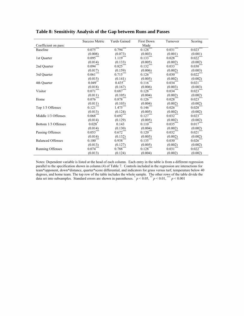
Table 8: Sensitivity Analysis of the Gap between Runs and Passes

Coefficient on pass:

Success Metric Yards Gained First Down Made

Turnover Scoring

Baseline 0.075*** 0.794*** 0.128*** 0.031*** 0.023*** (0.008) (0.073) (0.003) (0.001) (0.001) 1st Quarter 0.095*** 1.119*** 0.133*** 0.028*** 0.022*** (0.014) (0.133) (0.005) (0.002) (0.002) 2nd Quarter 0.094*** 0.825*** 0.132*** 0.033*** 0.030*** (0.017) (0.159) (0.006) (0.002) (0.003) 3rd Quarter 0.061*** 0.715*** 0.126*** 0.030*** 0.022*** (0.015) (0.141) (0.005) (0.002) (0.002) 4th Quarter 0.049** 0.435** 0.116*** 0.034*** 0.021*** (0.018) (0.167) (0.006) (0.003) (0.003) Visitor 0.071*** 0.687*** 0.128*** 0.034*** 0.023*** (0.011) (0.105) (0.004) (0.002) (0.002) Home 0.076*** 0.878*** 0.126*** 0.028*** 0.023*** (0.011) (0.103) (0.004) (0.002) (0.002) Top 1/3 Offenses 0.121*** 1.475*** 0.146*** 0.026*** 0.028*** (0.013) (0.124) (0.005) (0.002) (0.002) Middle 1/3 Offenses 0.068*** 0.692*** 0.127*** 0.032*** 0.023*** (0.014) (0.129) (0.005) (0.002) (0.002) Bottom 1/3 Offenses 0.028* 0.143 0.110*** 0.035*** 0.017*** (0.014) (0.130) (0.004) (0.002) (0.002) Passing Offenses 0.053*** 0.672*** 0.120*** 0.032*** 0.021*** (0.014) (0.132) (0.005) (0.002) (0.002) Balanced Offenses 0.100*** 0.938*** 0.135*** 0.030*** 0.026*** (0.013) (0.127) (0.005) (0.002) (0.002) Running Offenses 0.074*** 0.788*** 0.128*** 0.031*** 0.022*** (0.013) (0.124) (0.004) (0.002) (0.002) Notes: Dependent variable is listed at the head of each column. Each entry in the table is from a different regression parallel to the specification shown in column (4) of Table 7. Controls included in the regression are interactions for team*opponent, down*distance, quarter*score differential, and indicators for grass versus turf, temperature below 40 degrees, and home team. The top row of the table includes the whole sample. The other rows of the table divide the data set into subsamples. Standard errors are shown in parentheses. * p < 0.05, ** p < 0.01, *** p < 0.001

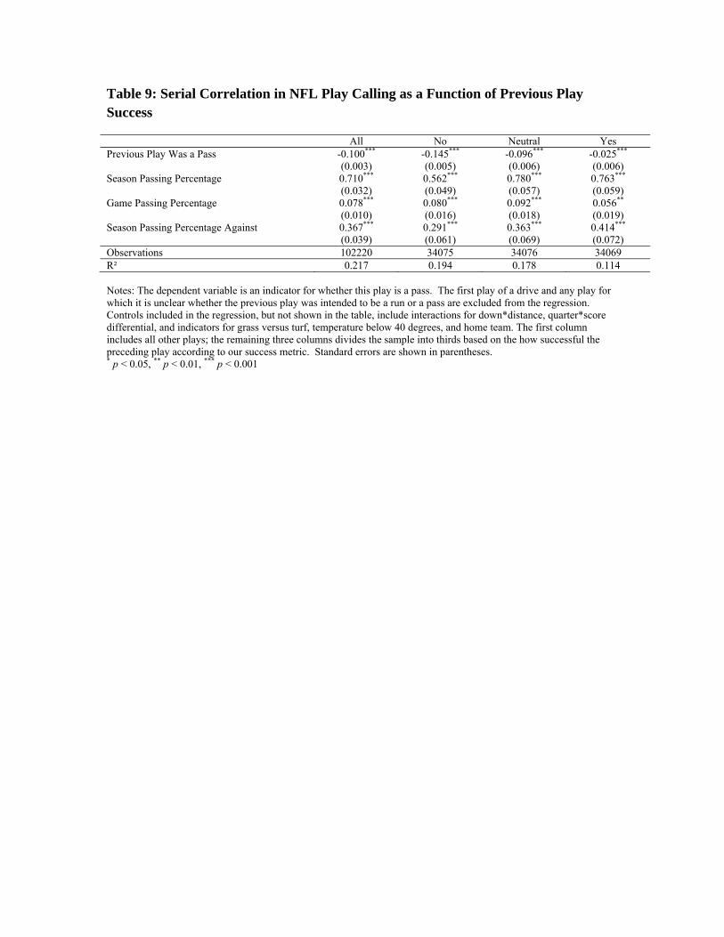
Table 9: Serial Correlation in NFL Play Calling as a Function of Previous Play Success

All No Neutral Yes Previous Play Was a Pass -0.100*** -0.145*** -0.096*** -0.025*** (0.003) (0.005) (0.006) (0.006) Season Passing Percentage 0.710*** 0.562*** 0.780*** 0.763*** (0.032) (0.049) (0.057) (0.059) Game Passing Percentage 0.078*** 0.080*** 0.092*** 0.056** (0.010) (0.016) (0.018) (0.019) Season Passing Percentage Against 0.367*** 0.291*** 0.363*** 0.414*** (0.039) (0.061) (0.069) (0.072) Observations 102220 34075 34076 34069 R² 0.217 0.194 0.178 0.114 Notes: The dependent variable is an indicator for whether this play is a pass. The first play of a drive and any play for which it is unclear whether the previous play was intended to be a run or a pass are excluded from the regression. Controls included in the regression, but not shown in the table, include interactions for down*distance, quarter*score differential, and indicators for grass versus turf, temperature below 40 degrees, and home team. The first column includes all other plays; the remaining three columns divides the sample into thirds based on the how successful the preceding play according to our success metric. Standard errors are shown in parentheses. * p < 0.05, ** p < 0.01, *** p < 0.001

References

Brayer, A.R. 1964. An experimental analysis of some variables of minimax theory.

Behavioral Science 9 (1): 33–44. Brown, J.N., and R.W. Rosenthal. 1990. Testing the minimax hypothesis: A re-

examination of O'Neill's game experiment. Econometrica 58(5): 1065–1081. Budescu, D.V., and A. Rapoport. 1992. Generation of random series in two-person

strictly competitive games. Journal of Experimental Psychology 121 (3): 352-363. Chiappori, P.A., S. Levitt, and T. Groseclose. 2002. Testing mixed strategy equilibria

when players are heterogeneous: The case of penalty kicks in soccer. AmericanEconomic Review 92 (4):1138–1151.

Fox, J. 1972. The learning of strategies in a simple, two-person zero-sum game without

saddlepoint. Behavioural Science. 17 (3): 300–308. Fox, Dan, 2006, “Run Estimation for the Masses,” posted at

http://www.hardballtimes.com/main/article/ops-for-the-masses/ and accessed on July 21, 2009.

Hsu, S-H., C-Y. Huang, and C-T. Tang. 2007. Minimax play at Wimbledon: Comment.

The American Economic Review 97 (1): 517-523. Levitt, S., 2006, “An Economist Sells Bagels: A Case Study in Profit Maximiation,”

NBER Working Paper 12152. Levitt, S., and J. List. 2007. What do laboratory experiments measuring social

preferences reveal about the real world? Journal of Economic Perspectives 21 (2): 153-174.

Lieberman, B. 1960. Human behavior in a strictly determined 3 × 3 matrix game.

Behavioral Science 5(4): 317–322. Lieberman, B. 1962. “Experimental studies of conflict in some two-person and three

person games.” In Mathematical Models in Small Group Processes, edited by J.H. Criswell, H. Solomon, and P. Suppes. Stanford, CA: Stanford University Press. 203–220.

Messick, D.M. 1967. Interdependent decision strategies in zero-sum games: A computer

controlled study. Behavioral Science 12 (1): 33–48. O'Neill, B. 1987. A non-metric test of the minimax theory of two-person zerosum games.

Proceedings of the National Academy of Sciences 84 (7): 2106-2109.

O'Neill, B. 1991. Comments on Brown and Rosenthal’s reexamination. Econometrica 59

(2): 503-507. Palacios-Huerta, I. 2003. Professionals play minimax. Review of Economic Studies 70

(2): 395-415. Palacios-Huerta, I. and O. Volij. 2007. Experientia docet: Professionals play minimax in

laboratory experiments. Econometrica (forthcoming). Pope, Devin, and Maurice Schweitzer, 2009, “Is Tiger Woods Loss Averse? Persistent

Bias in the Face of Experience, Competition, and High Stakes,” Unpublished manuscript.

Romer, David, “Do Firms Maximize? Evidence from Professional Football,” Journal of

Political Economy 114(2): 340-365. Rosenthal, R.W., J. Shachat, and M. Walker. 2003. Hide and seek in Arizona.

International Journal of Game Theory 32 (2): 273-293. Shachat, J., and T.J. Swarthout. 2004. Do we detect and exploit mixed strategy play by

opponents? Mathematical Methods of Operations Research 59 (3): 359-373. Spiliopoulos, L. 2007. Do repeated game players detect patterns in opponents? Revisiting

the Nyarko and Schotter belief elicitation experiment. Munich Personal RePEc Archive Paper No. 2179. http://mpra.ub.uni-muenchen.de/2179.

Walker, M., and J. Wooders. 2001. Minimax play at Wimbledon. American Economic

Review 91 (5): 1521–38.