professor fadzlan sufian, phd iium institute of islamic ... eng/fadzlan_sufian.pdf · professor...
TRANSCRIPT

Professor Fadzlan SUFIAN, PhD
IIUM Institute of Islamic Banking and Finance
International Islamic University
Malaysia
E-mail: [email protected]; [email protected]
FINANCIAL REPRESSION, LIBERALIZATION AND BANK TOTAL
FACTOR PRODUCTIVITY: EMPIRICAL EVIDENCE FROM THE
THAILAND BANKING SECTOR
Abstract. The present paper employs the Malmquist Productivity Index (MPI)
method to examine sources of total factor productivity change of the Thailand
banking sector during the post-Asian financial crisis period of 1999-2008. The
empirical findings suggest that the Thailand banking sector has exhibited
productivity regress during the period under study due to technological regress. The
results indicate that the domestic banks have exhibited productivity regress due to
technological regress, while the foreign banks have exhibited productivity progress
attributed to technological progress. Credit risk and diversification have negative
impacts on Thailand banks’ total factor productivity. On the other hand, the better
capitalized and profitable Thailand banks tend to be relatively more productive.
During the period under study, business cycle display mixed impacts. The empirical
findings seem to suggest that the different structures of bank ownership have no
significant impact on bank productivity.
Keywords: Banks, Total Factor Productivity, Malmquist Productivity Index,
Panel Regression Analysis, Thailand.
JEL Classification: G21
1.0 INTRODUCTION Banks play significant roles in mobilizing savings to fuel investments and
growth. This role is particularly significant in Thailand where banks continue to
dominate the financial markets. As at end- 2008, banks accounts for 64.2% of the
financial system’s total assets. Expansionary economic activities by corporations and
the government are mostly financed by the banking sector. About 61.1% of the credit
requirements of local companies in Thailand are supplied by banks, while only 32.4%
Fadzlan Sufian
____________________________________________________________________
by the capital markets. The dominance of banks can be explained by many factors,
among others the underdevelopment of the capital markets.
Apart from its role in financial intermediation, banks have been shown to
contribute to general economic stability. This integral link was evident during the
Asian financial crisis, where the Thailand economy was adversely affected when
banks have been weak and vulnerable to external shocks. Earlier studies have
suggested that fragilities in the banking system played key roles in propagating the
financial crisis that halted the momentum of the so-called East Asian growth miracle
in the mid-1990. The crisis caused the affected economies, as well as Thailand, to
slow down arising from among others the pull out of investors, currency
depreciations, higher interest rates, and large debt overhang.
Since the Asian financial crisis, a number of significant changes have
occurred in the Thailand banking sector as a result of its adaptation to new conditions
such as the deregulation of the national markets and the internationalization of
competition. To develop Thailand as a regional financial center, the central bank,
Bank of Thailand (BOT) has allowed qualified financial institutions operating the
Bangkok International Banking Facilities (BIBFs) since 1993 and in other provinces
(PIBFs) since 1994. A license for international banking facilities permits domestic
commercial banks and foreign bank branches to provide acceptance of deposits in
foreign currencies, lending in foreign currencies to both residents (out-in lending) and
non-residents (out-out lending), and foreign exchange transactions. That is,
mobilization of foreign savings to finance the country’s economic growth has become
more flexible. In 1998, 10 Thai banks and 35 foreign bank branches have been
granted permission to establish BIBF offices, while another 23 foreign bank branches
are allowed to get PIBF licenses in other provinces.
It is reasonable to assume that these developments posed great challenges to
banks operating in the Thailand banking sector as the environment in which they
operate changed rapidly. Golin (2001) points out that, adequate earnings are required
in order for banks to maintain solvency, to survive, grow, and prosper in a
competitive environment. Furthermore, the earlier studies by among others Rajan and
Zingales (1998) showed that there is a close relationship between the growth of the
economy and the well being of the banking sector. Therefore, knowledge of the
underlying factors that influence the performance of the banking sector is essential
not only for the managers of the banks, but for numerous stakeholders such as the
central bank, bankers association, the government, and other financial authorities.
Knowledge of these factors would be helpful for the regulatory authorities and bank
managers to formulate going forward policies for the Thailand banking sector.
By using the whole gamut of commercial banks operating in the Thailand
banking sector, the present paper seeks to examine the performance of the Thailand
banking sector during the post Asian financial crisis period of 1999-2008, which is
characterized as a time of significant restructuring in the country’s financial sector.

Financial Repression, Liberalization and Bank Total Factor Productivity…………….
_____________________________________________________________________
The paper also investigates to what extent the performance of commercial banks is
influenced by internal factors (i.e. bank specific characteristics) and to what extent by
external factors (i.e. macroeconomic and banking sector conditions). We differentiate
this paper from the previous ones that focus on the Thailand banking sector and
contribute to the present literature in at least three important ways.
Firstly, we employ two different estimating principles. The DEA based
Malmquist Productivity Index (MPI) method, which is one of the techniques we
employ, is a non-parametric and oriented to frontier rather than central tendency
estimates (Cooper et al. 2006). Unlike the previous studies focusing on the Thailand
banking sector, the present study adopts a dynamic panel of the MPI method.
Furthermore, Isik and Hassan (2002) point out that the dynamic panel is more
flexible and thus more appropriate than estimating a single multiyear frontier for the
banks in the sample.
Secondly, following the more recent approach suggested by Chang et al.
(2009) among others, we also use the central tendency and parametric method that
are involved in a random effects panel regression analysis to investigate the Thailand
banking sector’s production efficiency, while controlling for the potential effects of
the contextual variables. In this way, we protect against the ‘methodological bias’
that can occur when only one method is used (see the exchange between Evans and
Heckman (1988) and Charnes et al. (1988)). Although this approach has been used in
some of the earlier studies, in our case we examine a more recent period that follows
the changes outlined above.
This paper is structured as follows. The next section reviews the related
studies in the literature. In section 3, we outline the approaches to the measurement
and estimation of total factor productivity change, justify our use of what is called the
“intermediation approach” to the measurement of bank inputs and outputs, outlines
the econometric framework, and provide details on the construction of our data set.
Section 4 discusses the results, and finally section 6 provides some concluding
remarks and policy implications.
2.0 A BRIEF REVIEW OF RELATED LITERATURE
Since its introduction by Charnes et al. (1978) and Banker et al. (1984),
researchers have welcomed Data Envelopment Analysis (DEA) as a methodology for
performance evaluation (Gregoriou and Zhou, 2005). However, a large body of
literature exists on banking efficiency in the United States (see surveys by Berger and
Humphrey, 1997; Berger, 2007 and references therein) and the banking systems in
the western and developed countries (Sathye, 2001; Hauner, 2005; Pasiouras, 2008;
etc). On the other hand, relatively few have been conducted within the developing
economies banking sectors (Berger and Humphrey, 1997).
Despite substantial studies performed in regard to the efficiency and
productivity of financial institutions in the U.S., Europe, and other developed

Fadzlan Sufian
____________________________________________________________________
countries banking sectors, empirical evidences on the developing countries banking
sectors, particularly Thailand are relatively scarce. To date, the studies by Leightner
and Lovell (1998) and Williams and Intrachote (2003) are the two most notable
empirical research performed to examine the efficiency of the Thailand banking
sector. The earlier study by Leightner and Lovell (1998) found mixed performance of
the foreign owned banks during the period of 1989 to 1994. They suggest that the
large domestically owned banks to be the most efficient, while the foreign owned
banks have exhibited slightly higher efficiency level compared to the medium sized
domestic owned banks. The smaller domestic owned banks were found to be the most
inefficient banks.
A more recent study by Williams and Intrachote (2003) conclude that the
efficiency of the foreign and domestic owned banks during the period of 1990 to
1997 were comparable. By employing the Stochastic Frontier Approach (SFA), they
found that the Japanese owned banks in Thailand to be significantly more efficient
compared to their domestic owned bank counterparts and foreign banks from other
nations. Their results supports to the view that foreign owned banks from strong
home environments may carry efficiency advantages overseas.
The above literature reveals the following research gaps. First, the majority of
these studies concentrate on the banking sectors of the developed countries, such as
the U.S., Europe and other developed countries banking sectors. Second, empirical
evidence on the developing and emerging countries are relatively scarce. Finally,
apart from the few studies discussed above, virtually nothing has been published to
examine the sources of total factor productivity of the Thailand banking sector during
the post-Asian financial crisis period. In the light of these knowledge gaps, this paper
seeks to provide new empirical evidence on the sources of total factor productivity
change in the Thailand banking sector.
3.0 METHODOLOGY AND DATA
3.1 Malmquist Productivity Index (MPI)
Three different indices are frequently used to evaluate total factor productivity
changes: the Fischer (1922), Tornqvist (1936), and Malmquist (1953) indices. The
non-parametric (Malmquist) and parametric (Fischer and Tornqvist) indices differ in
several ways in respect to their behavioural assumptions and whether or not they
recognize random errors in the data (noise). Grifell-Tatje and Lovell (1996) suggest
that the Malmquist Productivity Index (MPI) has several distinct advantages over the
Fischer and Tornqvist indices.
Firstly, it does not require the profit maximization, or the cost minimization
assumption. Secondly, it does not require information on the input and output prices.
Thirdly, if the researcher has panel data, it allows the decomposition of productivity
changes into two components (technical efficiency change or catching up and

Financial Repression, Liberalization and Bank Total Factor Productivity…………….
_____________________________________________________________________
technical change or changes in the best practice). Finally, unlike the parametric
methods, it does not require specifying the functional form for the frontier, which
could be biased due to specification errors if the functional form is mis-specified. Its
main disadvantage is the necessity to compute the distance functions. However, the
Data Envelopment Analysis (DEA) technique can be used to solve this problem.
Following Fare et al. (1994) among others, the present study adopts the output
oriented Malmquist Productivity Index (MPI). The analysis employs the notion of an
output distance function first proposed by Shephard (1970), which measures how
much a unit’s outputs can be proportionately increased given the observed levels of
its inputs. The structure of the production technology is assumed to exhibit constant
returns to scale (CRS). We delineate the structure of production technology with the
output distance function as follows:
{ }( , ) min | ( , )t t t t t t
j j j jD x y x y Pφ φ= ∈ , (1)
which measures the output technical efficiency of bank j at time t relative to
the technology at time t (Shephard, 1970). Since technical efficiency is measured
relative to the contemporaneous technology, we have ( , ) 1t t t
j jD X Y ≤ , with
( , ) 1t t t
j jD X Y = signifying that unit j is on the production frontier and is technically
efficient, while ( , ) 1t t t
j jD X Y < indicating that the unit is below the frontier and is
technically inefficient.
Before describing the MPI method, we need to define distance functions with
respect to two different time periods. The efficiency of unit j at time t relative to the
technology at time t+1 is represented by
{ }1 1( , ) min | ( , )t t t t t t
j j j jD x y x y Pφ φ+ += ∈ . (2)
Similarly, the efficiency of unit j at time t+1 relative to the technology at time
t is defined by the distance function
{ }1 1 1 1( , ) min | ( , )t t t t t t
j j j jD x y x y Pφ φ+ + + += ∈ . (3)
Caves et al. (1982) define the MPI as
),(
),(),,,(
11
11
t
j
t
j
t
t
j
t
j
t
t
j
t
j
t
j
t
j
t
yxD
yxDyxyxM
++++ =
or
Fadzlan Sufian
____________________________________________________________________
),(
),(),,,(
1
111
111
t
j
t
j
t
t
j
t
j
t
t
j
t
j
t
j
t
j
t
yxD
yxDyxyxM
+
++++++ =
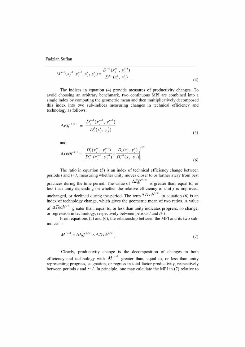
. (4)
The indices in equation (4) provide measures of productivity changes. To
avoid choosing an arbitrary benchmark, two continuous MPI are combined into a
single index by computing the geometric mean and then multiplicatively decomposed
this index into two sub-indices measuring changes in technical efficiency and
technology as follows:
),(
),( 111
1,
t
j
t
j
t
c
t
j
t
j
t
ctt
yxD
yxDEff
++++ =∆
(5)
and 21
1111
11
1,
),(
),(
),(
),(
×=∆
++++
+++
t
j
t
j
t
c
t
j
t
j
t
c
t
j
t
j
t
c
t
j
t
j
t
ctt
yxD
yxD
yxD
yxDTech
. (6)
The ratio in equation (5) is an index of technical efficiency change between
periods t and t+1, measuring whether unit j moves closer to or farther away from best
practices during the time period. The value of , 1t tEff +∆
is greater than, equal to, or
less than unity depending on whether the relative efficiency of unit j is improved,
unchanged, or declined during the period. The term, 1t tTech +∆ in equation (6) is an
index of technology change, which gives the geometric mean of two ratios. A value
of , 1t tTech +∆ greater than, equal to, or less than unity indicates progress, no change,
or regression in technology, respectively between periods t and t+1.
From equations (5) and (6), the relationship between the MPI and its two sub-
indices is
1,1,1, +++ ∆×∆= tttttt TechEffM . (7)
Clearly, productivity change is the decomposition of changes in both
efficiency and technology with , 1t tM +
greater than, equal to, or less than unity
representing progress, stagnation, or regress in total factor productivity, respectively
between periods t and t+1. In principle, one may calculate the MPI in (7) relative to

Financial Repression, Liberalization and Bank Total Factor Productivity…………….
_____________________________________________________________________
any technology pattern. The CRS technology is adopted to compute the MPI and its
two sub-indices in the preceding analysis.
The , 1t tEff +∆
index can be further disaggregated into its mutually exhaustive
components of pure technical efficiency change , 1t tPureEff +∆ calculated relative to
the variable returns to scale (VRS) technology and a component of scale efficiency
change , 1t tScale +∆ capturing changes in the deviation between the VRS and CRS
technologies. That is,
1,1,1, +++ ∆×∆=∆ tttttt ScalePureEffEff , (8)
where 1 1 1
, 1( , )
( , )
t t t
v j jt t
t t t
v j j
D x yPureEff
D x y
+ + ++∆ =
, (9)
),(),(
),(),( 111111
1,
t
j
t
j
t
v
t
j
t
j
t
c
t
j
t
j
t
v
t
j
t
j
t
ctt
yxDyxD
yxDyxDScale
+++++++ =∆
(10)
The subscripts “v” and “c” denote VRS and CRS technologies, respectively. , 1 1t tPureEff +∆ > indicates an increase in pure technical efficiency, while
, 1 1t tPureEff +∆ < indicates a decrease and , 1 1t tPureEff +∆ = indicates no change in
pure technical efficiency. Similarly, , 1 1t tScale +∆ > implies that the most efficient
scale is increasing over time, so the scale efficiency is improving, while , 1 1t tScale +∆ < implies the opposite, and
, 1 1t tScale +∆ = indicates that there is no
change in scale efficiency.
3.2 Specification of Bank Inputs, Outputs
The definition and measurement of inputs and outputs in the banking function
remains a contentious issue among researchers. In the banking theory literature, there
are two main approaches competing with each other in this regard: the production and
intermediation approaches (Sealey and Lindley, 1977). Under the production
approach, pioneered by Benston (1965), a financial institution is defined as a
producer of services for account holders, that is, they perform transactions on deposit
accounts and process documents such as loans. The intermediation approach on the
other hand assumes that financial firms act as an intermediary between savers and
borrowers and posits total loans and securities as outputs, whereas deposits along
with labour and physical capital are defined as inputs.
Fadzlan Sufian
____________________________________________________________________
For the purpose of this study, a variation of the intermediation approach or
asset approach originally developed by Sealey and Lindley (1977) will be adopted in
the definition of inputs and outputs used. According to Berger and Humphrey (1997),
the production approach might be more suitable for branch efficiency studies as at
most times bank branches process customer documents and bank funding, while
investment decisions are mostly not under the control of branches.
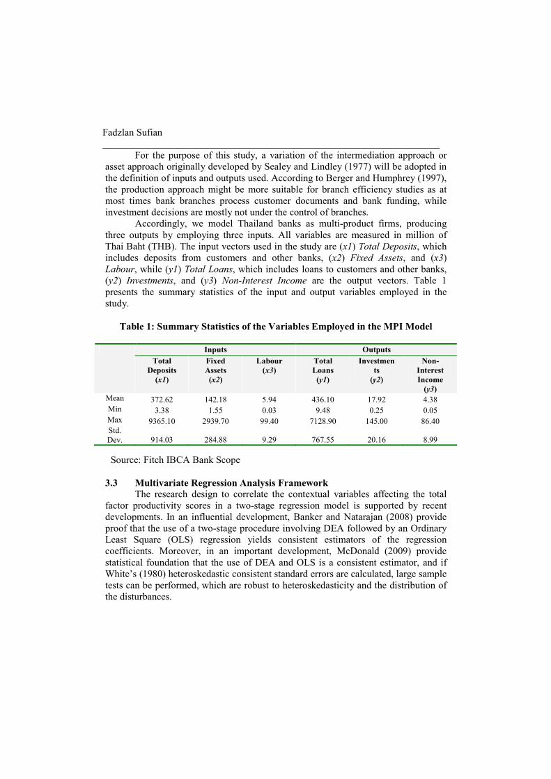
Accordingly, we model Thailand banks as multi-product firms, producing
three outputs by employing three inputs. All variables are measured in million of
Thai Baht (THB). The input vectors used in the study are (x1) Total Deposits, which
includes deposits from customers and other banks, (x2) Fixed Assets, and (x3)
Labour, while (y1) Total Loans, which includes loans to customers and other banks,
(y2) Investments, and (y3) Non-Interest Income are the output vectors. Table 1
presents the summary statistics of the input and output variables employed in the
study.
Table 1: Summary Statistics of the Variables Employed in the MPI Model
Inputs Outputs
Total
Deposits
(x1)
Fixed
Assets
(x2)
Labour
(x3)
Total
Loans
(y1)
Investmen
ts
(y2)
Non-
Interest
Income
(y3) Mean 372.62 142.18 5.94 436.10 17.92 4.38
Min 3.38 1.55 0.03 9.48 0.25 0.05
Max 9365.10 2939.70 99.40 7128.90 145.00 86.40
Std.
Dev. 914.03 284.88 9.29 767.55 20.16 8.99
Source: Fitch IBCA Bank Scope
3.3 Multivariate Regression Analysis Framework
The research design to correlate the contextual variables affecting the total
factor productivity scores in a two-stage regression model is supported by recent
developments. In an influential development, Banker and Natarajan (2008) provide
proof that the use of a two-stage procedure involving DEA followed by an Ordinary
Least Square (OLS) regression yields consistent estimators of the regression
coefficients. Moreover, in an important development, McDonald (2009) provide
statistical foundation that the use of DEA and OLS is a consistent estimator, and if
White’s (1980) heteroskedastic consistent standard errors are calculated, large sample
tests can be performed, which are robust to heteroskedasticity and the distribution of
the disturbances.
Financial Repression, Liberalization and Bank Total Factor Productivity…………….
_____________________________________________________________________
Thus, following Banker and Natarajan (2008) among others, equation (11) is
estimated by using the Ordinary Least Square (OLS) method. As suggested by
McDonald (2009), we estimate equation (11) by using White (1980) transformation,
which is robust to heteroskedasticity and the distribution of the disturbances in the
second stage regression analysis. In order to check for the robustness of the results,
following Chang et al. (2009) among others, we control for bank specific effects by
applying the least square method of the random effects (RE) model. The opportunity
to use a random effects rather than a fixed effects model has been tested with the
Hausman test. The standard errors are again computed by using White’s (1980)
transformation to control for cross section heteroscedasticity of the variables.
By using the TFPCH scores as the dependent variable, the following
regression model is estimated:
λjt = δ0 + β1LLP/TLjt + β2NII/TAjt + β3NIE/TAjt + β4LOANS/TAjt (11)
+ β5LNTAjt + β6EQASSjt + β7ROAjt
+ ζ 1LNGDPt + ζ 2INFLt + ζ 3CR3t + ζ 4MKTCAP/GDPt
+ δ 1DUMFORBj + δ 2DUMGOVTj + δ 3DUMPUBLj
+ ε jt
where ‘i’ denotes the bank, ‘t’ the examined time period, and ε is the disturbance term,
with vit capturing the unobserved bank specific effect and uit is the idiosyncratic error
and is independently identically distributed (i.i.d), ),0(~2σNeit .
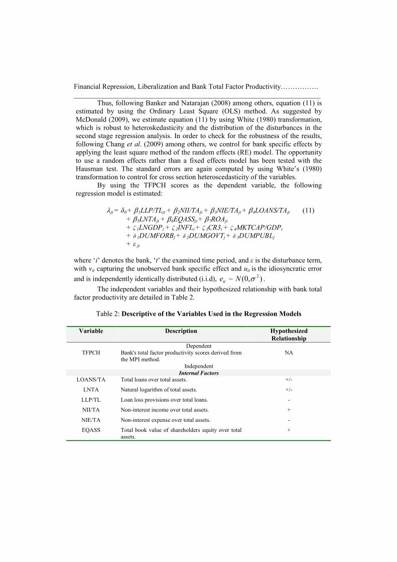
The independent variables and their hypothesized relationship with bank total
factor productivity are detailed in Table 2.
Table 2: Descriptive of the Variables Used in the Regression Models
Variable Description Hypothesized
Relationship
Dependent
TFPCH Bank's total factor productivity scores derived from
the MPI method.
NA
Independent
Internal Factors LOANS/TA Total loans over total assets. +/-
LNTA Natural logarithm of total assets. +/-
LLP/TL Loan loss provisions over total loans. -
NII/TA Non-interest income over total assets. +
NIE/TA Non-interest expense over total assets. -
EQASS Total book value of shareholders equity over total
assets.
+
Fadzlan Sufian
____________________________________________________________________
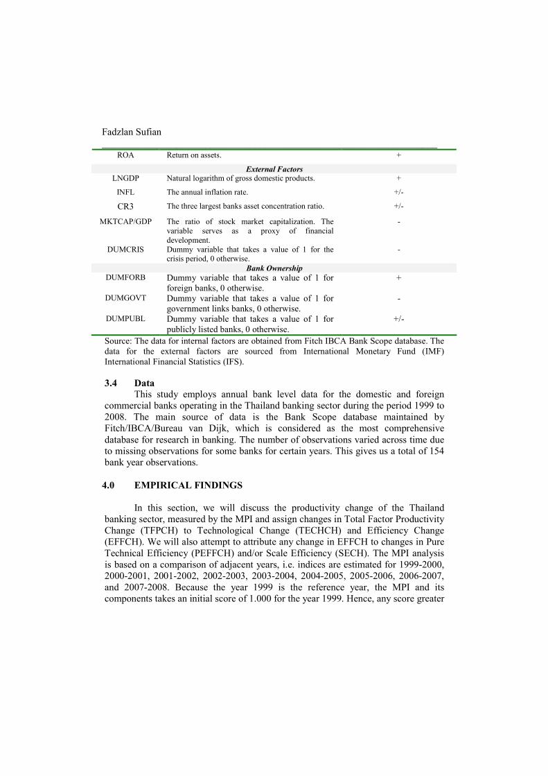
ROA Return on assets. +
External Factors LNGDP Natural logarithm of gross domestic products. +
INFL The annual inflation rate. +/-
CR3 The three largest banks asset concentration ratio. +/-
MKTCAP/GDP
The ratio of stock market capitalization. The
variable serves as a proxy of financial
development.
-
DUMCRIS Dummy variable that takes a value of 1 for the
crisis period, 0 otherwise.
-
Bank Ownership DUMFORB Dummy variable that takes a value of 1 for
foreign banks, 0 otherwise.
+
DUMGOVT Dummy variable that takes a value of 1 for
government links banks, 0 otherwise.
-
DUMPUBL Dummy variable that takes a value of 1 for
publicly listed banks, 0 otherwise.
+/-
Source: The data for internal factors are obtained from Fitch IBCA Bank Scope database. The
data for the external factors are sourced from International Monetary Fund (IMF)
International Financial Statistics (IFS).
3.4 Data
This study employs annual bank level data for the domestic and foreign
commercial banks operating in the Thailand banking sector during the period 1999 to
2008. The main source of data is the Bank Scope database maintained by
Fitch/IBCA/Bureau van Dijk, which is considered as the most comprehensive
database for research in banking. The number of observations varied across time due
to missing observations for some banks for certain years. This gives us a total of 154
bank year observations.
4.0 EMPIRICAL FINDINGS
In this section, we will discuss the productivity change of the Thailand
banking sector, measured by the MPI and assign changes in Total Factor Productivity
Change (TFPCH) to Technological Change (TECHCH) and Efficiency Change
(EFFCH). We will also attempt to attribute any change in EFFCH to changes in Pure
Technical Efficiency (PEFFCH) and/or Scale Efficiency (SECH). The MPI analysis
is based on a comparison of adjacent years, i.e. indices are estimated for 1999-2000,
2000-2001, 2001-2002, 2002-2003, 2003-2004, 2004-2005, 2005-2006, 2006-2007,
and 2007-2008. Because the year 1999 is the reference year, the MPI and its
components takes an initial score of 1.000 for the year 1999. Hence, any score greater

Financial Repression, Liberalization and Bank Total Factor Productivity…………….
_____________________________________________________________________
(lower) than 1.000 in subsequent years indicates an improvement (deterioration) in
the relevant measure.
It is also worth mentioning that favorable efficiency change (EFFCH) is
interpreted as evidence of “catching up” to the frontier, while favorable technological
change (TECHCH) is interpreted as innovation (Cummins et al. 1999). Panels A, B,
and C of Table 3 present the summary of annual means for the industry, the domestic,
and foreign banks TFPCH, TECHCH, EFFCH, and its decomposition into PEFFCH
and SECH for the years 1999-2008 respectively.
4.1 Total Factor Productivity Growth of Thailand Banks As depicted in Panel A of Table 3, the MPI results suggest that during the
period of 1999-2008, on average, the Thailand banking sector has exhibited
productivity regress of 0.9%. The empirical findings from this study suggest that the
Thailand banking sector has exhibited productivity decline during the years 2000,
2002, 2005, and 2008, while productivity was observed to have increased during the
years 2001, 2003, 2004, and 2007. It is also observed from Panel A of Table 3 that
the Thailand banking sector’s productivity was stagnant during the year 2006. During
the period under study, the decline in the Thailand banking sector’s productivity was
mainly due to technological change regress rather than efficiency change decline. The
decomposition of the efficiency change index into its pure technical and scale
efficiency components suggest that the source of the increase in Thailand banking
sector’s efficiency was mainly attributed to pure technical rather than scale
efficiency, implying that Thailand banks have been managerially efficient in
controlling their operating costs, but have been operating at the non-optimal scale of
operations.
Panel B of Table 3 presents the results for the domestic banks. As observed,
during the period under study, the empirical findings seem to suggest that the
domestic banks have exhibited productivity regress of 1.9%. The decomposition of
the productivity change index into its technological and efficiency change
components suggest that the domestic banks’ productivity were adversely affected by
the regress in technological change of 2.6% during the years. The decomposition of
the efficiency change index into its pure technical and scale efficiency components
suggest that the dominant source of the increase in the domestic banks’ efficiency
were solely attributed to pure technical efficiency. This implies that although the
domestic banks have been efficient in controlling their operating costs, they have
been operating at the non-optimal scale of operations.
The results for the foreign banks operating in Thailand are presented in Panel
C of Table 3. During the period under study, the results seem to indicate that the
foreign banks have exhibited productivity progress of 3.0%. Unlike their domestic
bank counterparts, the decomposition of the productivity change index into its
mutually exhaustive components of technological and efficiency change suggest that
the foreign banks have exhibited productivity progress mainly attributed to the
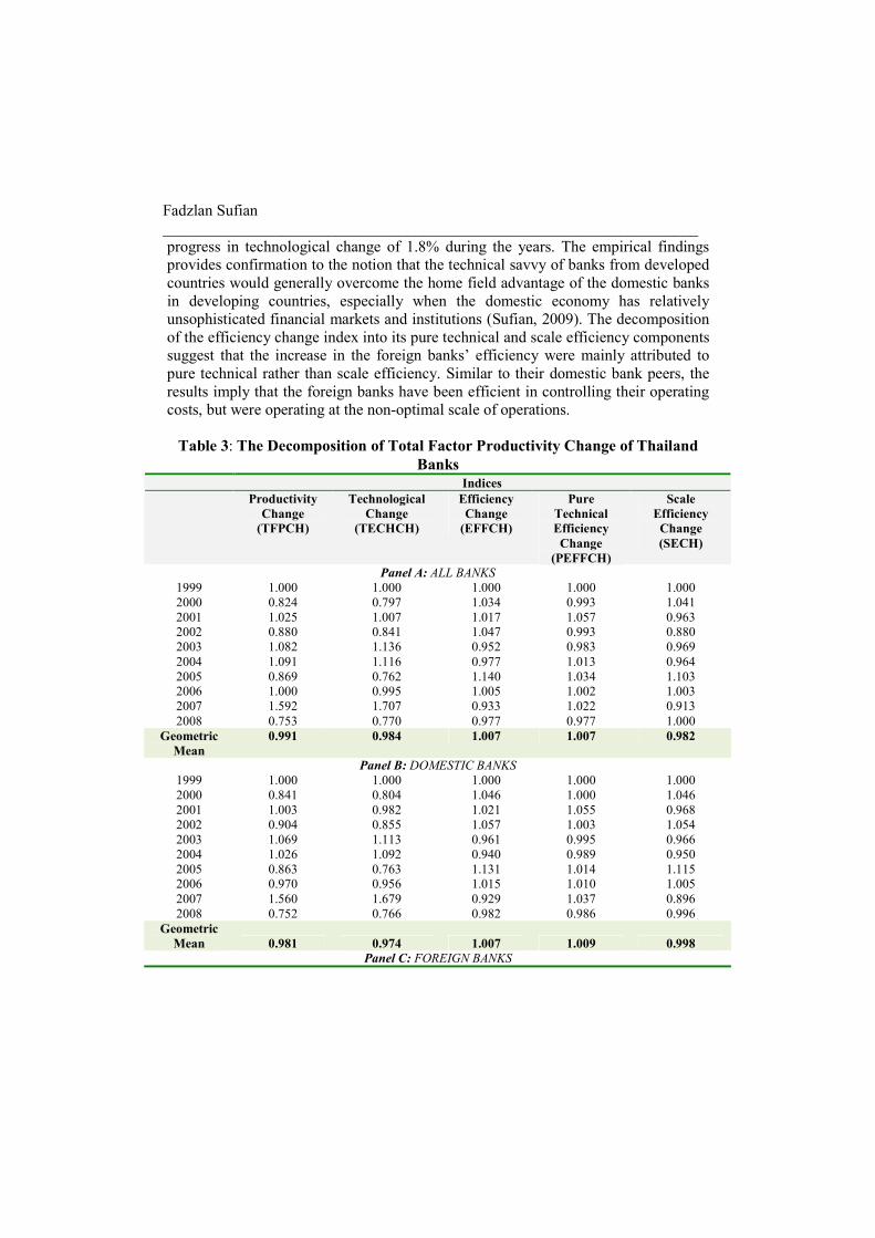
Fadzlan Sufian
____________________________________________________________________
progress in technological change of 1.8% during the years. The empirical findings
provides confirmation to the notion that the technical savvy of banks from developed
countries would generally overcome the home field advantage of the domestic banks
in developing countries, especially when the domestic economy has relatively
unsophisticated financial markets and institutions (Sufian, 2009). The decomposition
of the efficiency change index into its pure technical and scale efficiency components
suggest that the increase in the foreign banks’ efficiency were mainly attributed to
pure technical rather than scale efficiency. Similar to their domestic bank peers, the
results imply that the foreign banks have been efficient in controlling their operating
costs, but were operating at the non-optimal scale of operations.
Table 3: The Decomposition of Total Factor Productivity Change of Thailand
Banks
Indices
Productivity
Change
(TFPCH)
Technological
Change
(TECHCH)
Efficiency
Change
(EFFCH)
Pure
Technical
Efficiency
Change
(PEFFCH)
Scale
Efficiency
Change
(SECH)
Panel A: ALL BANKS
1999 1.000 1.000 1.000 1.000 1.000
2000 0.824 0.797 1.034 0.993 1.041
2001 1.025 1.007 1.017 1.057 0.963
2002 0.880 0.841 1.047 0.993 0.880
2003 1.082 1.136 0.952 0.983 0.969
2004 1.091 1.116 0.977 1.013 0.964
2005 0.869 0.762 1.140 1.034 1.103
2006 1.000 0.995 1.005 1.002 1.003
2007 1.592 1.707 0.933 1.022 0.913
2008 0.753 0.770 0.977 0.977 1.000
Geometric
Mean
0.991 0.984 1.007 1.007 0.982
Panel B: DOMESTIC BANKS
1999 1.000 1.000 1.000 1.000 1.000
2000 0.841 0.804 1.046 1.000 1.046
2001 1.003 0.982 1.021 1.055 0.968
2002 0.904 0.855 1.057 1.003 1.054
2003 1.069 1.113 0.961 0.995 0.966
2004 1.026 1.092 0.940 0.989 0.950
2005 0.863 0.763 1.131 1.014 1.115
2006 0.970 0.956 1.015 1.010 1.005
2007 1.560 1.679 0.929 1.037 0.896
2008 0.752 0.766 0.982 0.986 0.996
Geometric
Mean 0.981 0.974 1.007 1.009 0.998
Panel C: FOREIGN BANKS

Financial Repression, Liberalization and Bank Total Factor Productivity…………….
_____________________________________________________________________
1999 1.000 1.000 1.000 1.000 1.000
2000 0.762 0.770 0.990 0.969 1.021
2001 1.105 1.102 1.004 1.062 0.944
2002 0.807 0.795 1.016 0.962 1.057
2003 1.126 1.216 0.926 0.944 0.980
2004 1.418 1.226 1.157 1.125 1.028
2005 0.896 0.760 1.180 1.119 1.055
2006 1.094 1.122 0.975 0.976 0.998
2007 1.679 1.783 0.942 0.983 0.959
2008 0.753 0.782 0.964 0.952 1.012
Geometric
Mean 1.030 1.018 1.012 1.007 1.005
Note: The mean scores of the Total Factor Productivity Change (TFPCH) index and its
components, Technological Change (TECHCH) and Efficiency Change (EFFCH) that is further
decomposed into Pure Technical Efficiency Change (PEFFCH) and Scale Efficiency Change
(SECH), for All Banks (ALL BANKS) and different forms in the sample, Domestic Banks
(DOMESTIC BANKS) and Foreign Banks (FOREIGN BANKS). Detailed results are available
from the authors upon request.
4.2 Factors Influencing Banks’ Total Factor Productivity
An important understanding that arises after the calculation of the MPI is to
attribute variations in productivity change to bank specific characteristics and the
environment in which they operate. Thus, the following section proceeds to discuss
the results derived from the multivariate regression analysis framework. The
regression results focusing on the relationship between bank total factor productivity
and the explanatory variables are presented in Table 4. To conserve space, the full
regression results, which include both bank and time specific random effects are not
reported in the paper. Several general comments regarding the test results are
warranted. The model performs reasonably well with most variables remain stable
across the various regressions tested. The explanatory power of the models is also
reasonably high and in most cases the F-statistics are also statistically significant at
the 5% level or better.
As expected, the coefficient of LLP/TL exhibits a negative sign when we
control for the recent global economic crisis and bank ownership forms. The results
suggest that Thailand banks with higher credit risks tend to exhibit lower total factor
productivity levels. If anything could be delved, the empirical findings imply that
Thailand banks should focus more on credit risk management, which has been proven
to be problematic in the recent past. Serious banking problems have arisen from the
failure of banks to recognize impaired assets and create reserves for writing off these
assets. An immense help towards smoothing these anomalies would be provided by
improving the transparency of the banking system, which in turn will assist banks to
evaluate credit risk more effectively and to avoid problems associated with hazardous
exposure.

Fadzlan Sufian
____________________________________________________________________
The coefficient of NII/TA has a negative sign and is statistically significant in
all regression models. The results imply that banks which derived a higher proportion
of its income from non-interest sources such as fee based services tend to be
relatively less productive. The finding is in consonance with the earlier study by
among others Stiroh (2006). To recap, Stiroh (2006) find that diversification benefits
of the U.S. financial holding companies are offset by the increased exposure to non-
interest activities, which are much more volatile, but not necessarily more profitable
than interest generating activities.
Referring to the impact of overhead costs on Thailand banks’ productivity, the
coefficient of NIE/TA consistently exhibits positive and statistically significant
impact on bank total factor productivity whether we control for the macroeconomic
and financial markets variables or not. The findings imply that an increase (decrease)
in these expenses results in a higher (lower) productivity of banks operating in the
Thailand banking sector. The results indicates that the more productive Thailand
banks tend to incur higher operating costs, which could be attributed to a more highly
qualified and professional management. Sathye (2001) points out that the more
highly qualified and professional management may require higher remuneration
packages, therefore a positive relationship with performance measures is normal.
The proxy measure of bank liquidity, LOANS/TA exhibits negative
relationship with bank productivity levels and is statistically significant when we
control for the recent global financial crisis and the various bank ownership
structures. The findings imply that banks with higher loans-to-asset ratios tend to be
more productive. Thus, in the case of the Thailand banking sector, bank loans seem to
be more highly valued than alternative bank outputs such as investments and
securities. The result is consistent with earlier studies by among others Molyneux and
Thornton (1992).
Concerning the impact of bank size, the coefficient of LNTA is negative
indicating an inverse relationship between total factor productivity and bank size.
Hauner (2005) offers two potential explanations for which size could have a positive
impact on bank performance. First, if it relates to market power, large banks should
pay less for their inputs. Second, there may be increasing returns to scale through the
allocation of fixed costs (e.g. research or risk management) over a higher volume of
services, or from efficiency gains from a specialized workforce. However, the results
need to be interpreted with caution since the coefficient of the variable has not been
statistically significant at any conventional levels in any of the regression models.
Capital strength as measured by EQASS is positively related to Thailand
banks’ total factor productivity. However, the coefficient of the variable is only
statistically significant when we control for the foreign (DUMFORB) and
government (DUMGOVT) own banks, but loses its explanatory power when we
control for the publicly listed banks (DUMPUBL). The empirical finding is
consistent with Pasiouras and Kosmidou (2007) providing support to the argument

Financial Repression, Liberalization and Bank Total Factor Productivity…………….
_____________________________________________________________________
that well capitalized banks face lower costs of going bankrupt, thus reduce their cost
of funding. Furthermore, strong capital structure is essential for bank in developing
economies, since it provides additional strength to withstand financial crises and
increased safety for depositors during unstable macroeconomic conditions (Sufian,
2009).
The empirical findings seem to suggest mixed impact of the indicators of
macroeconomic conditions on bank total factor productivity. The results about
LNGDP support the argument of the association between economic growth and the
performance of the banking sector. The high economic growth during the post-Asian
financial crisis period could have encouraged Thailand banks to lend more and
permits them to charge higher margins, as well as improving the quality of their
assets. On the other hand, the rate of inflation (INFL) is negatively related to
Thailand banks’ total factor productivity. The results imply that during the period
under study the levels of inflation have been unanticipated by Thailand banks
resulting in the banks’ costs to outpace their revenues and consequently had adverse
effects on performance.
Turning to the impact of the banking sector’s concentration, it is observed that
the coefficient of the three bank concentration ratio (CR_3) exhibits a negative sign.
However, it is worth noting that the coefficient of the variable is never significant in
any of the regression models estimated. On the other hand, the empirical findings
seem to suggest that the impact of stock market capitalization (MKTCAP/GDP) has a
negative relationship with Thailand banks’ TFPCH levels. If anything could be
delved, the findings seem to suggest that during the period under study, the Thailand
stock market serves as a complement rather than a substitute to borrowers in
Thailand. It is observed from column 3 of Table 4 that the coefficient of the
DUMCRIS variable is positive, but is not statistically significant at any conventional
levels.
The results presented in column 4 of Table 4 indicate that the coefficient of
DUMFORB is negative, but is not statistically significant at any conventional levels.
Similarly, the coefficient of DUMGOVT is negative, but again is not statistically
significant in the regression model estimated. During the period under study, the
empirical findings seem to suggest that there is no significant advantage accrued to
the publicly listed banks. The market discipline hypothesis implies that banks whose
shares are publicly traded should exhibit higher efficiency, but the findings from this
study seem to suggest that the Thailand capital market exerts no discipline over bank
management.

Fadzlan Sufian
____________________________________________________________________
Table 4: Panel Ordinary Least Square (OLS) Regression Analysis λjt = δ0 + β1LLP/TL + β2NII/TA + β3NIE/TA + β4LOANS/TA
+ β5LNTA + β6EQASS + β7ROA
+ ζ8LNGDP + ζ9INFL + ζ10CR3 + ζ11MKTCAP/GDP + ζ12DUMCRIS
+ δ13DUMFORB + δ14DUMGOVT + δ15DUMPUBL
+ εj
The dependent variable is bank's technical efficiency score derived from the MPI method. LLP/TL is a measure of banks
risk calculated as the ratio of total loan loss provisions divided by total loans. NII/TA is a measure of bank’s diversification towards non-interest income, calculated as total non-interest income divided by total assets. NIE/TA is a
measure of bank management quality calculated as total non-interest expenses divided by total assets. LOANS/TA is a
measure of bank’s loans intensity calculated as the ratio of total loans to bank total assets. LNTA is the size of the bank’s total asset measured as the natural logarithm of total bank assets. EQASS is a measure of banks capitalization measured
by banks total shareholders’ equity divided by total assets. ROA is return on assets calculated as profit after tax divided
by total assets. LNGDP is natural logarithm of gross domestic product. INFL is the rate of inflation. CR3 is the three largest banks asset concentration ratio. MKTCAP/GDP is the ratio of stock market capitalization. The variable serves as a
proxy of financial development. DUMCRIS is a dummy variable that takes a value of 1 for the crisis period, 0 otherwise.
DUMFORB is a dummy variable that takes a value of 1 for foreign banks, 0 otherwise. DUMGOVT is a dummy variable that takes a value of 1 for government links banks, 0 otherwise. DUMPUBL is a dummy variable that takes a value of 1
for publicly listed banks, 0 otherwise.
Values in parentheses are t-statistics.
***, **, and * indicate significance at 1, 5 and 10% levels.
(1) (2) (3) (4) (5) (6) CONSTANT 0.9787***
(6.1277)
0.4748
(0.3069)
3.5943**
(1.9567)
3.5394**
(1.9680)
3.4539**
(1.9548)
3.4656*
(1.8744)
Bank Specific Characteristics LLP/TL -0.0067
(-0.9216)
-0.0072
(-1.5006)
-0.0061**
(-2.0020)
-0.0051**
(-2.0212)
-0.0052**
(-2.1353)
-0.0050**
(-2.1226)
NII/TA -0.0619** (-2.4116)
-0.0571* (-1.6921)
-0.0753*** (-2.7376)
-0.0813*** (-3.0313)
-0.0847*** (-3.4512)
-0.0725*** (-2.7174)
NIE/TA 0.0292** (1.9847)
0.0206 (0.8560)
0.0310** (2.1315)
0.0302** (2.0041)
0.0298** (1.9390)
0.0261 (1.4550)
LOANS/TA 0.0003
(0.1773)
0.0002
(0.1637)
0.0005
(0.3412)
0.0010
(0.5128)
0.0011
(0.6297)
0.0005
(0.3264)
LNTA -0.0020
(-0.0793)
-0.0189
(-0.5008)
-0.0241
(-0.5477)
-0.0287
(-0.5984)
-0.0307
(-0.6231)
-0.0447
(-0.7522)
EQASS 0.0075 (0.7960)
0.0050 (0.7253)
0.1289** (2.1880)
0.1298** (2.1725)
0.1317** (2.0992)
0.0363 (0.7663)
ROA 0.0256
(1.2385)
0.0237
(1.0014)
0.0331**
(2.2929)
0.0323**
(2.2078)
0.0317**
(2.0945)
0.0259
(1.3887)
Economic and Market Conditions
LNGDP 0.5151*
(1.6435)
-0.4273
(-1.2795)
-0.4231
(-1.2776)
-0.4035
(-1.2261)
-0.4341
(-1.2714)
INFL -0.1906**
(-2.5682)
-0.0925***
(-2.6194)
-0.0910***
(-2.6075)
-0.0932**
(-2.6123)
-0.0779**
(-2.3049)
CR3 -4.1863
(-1.2999)
-1.5600
(-1.0221)
-1.4200
(-0.9485)
-1.4612
(-0.9826)
-0.9670
(-0.6900)
MKTCAP/GDP 0.0101** (2.5590)
0.0113*** (2.9148)
0.0112*** (2.9230)
0.0112*** (2.9276)
0.0108*** (2.9314)
DUMCRIS 0.0727
(1.0549)
Bank Ownership

Financial Repression, Liberalization and Bank Total Factor Productivity…………….
_____________________________________________________________________
DUMFORB -0.0257 (-0.6030)
DUMGOVT -0.0028 (-0.2391)
DUMPUBL 0.0360
(1.4286) No. of Obs. 154 154 154 154 154 154
R2 0.0562 0.3181 0.3760 0.3729 0.3726 0.4500 Adj. R2 0.0110 0.2653 0.3229 0.3195 0.3192 0.4032
D-W Statistics 2.7701 2.7380 1.9298 1.9583 1.9632 1.8602
F-Statistics 1.2431 6.0219*** 7.0810*** 6.9865*** 6.9771*** 9.6147***
4.3 Robustness Checks
In order to check for the robustness of the results, we have performed a
number of sensitivity analyses. First, we repeat equation (11) by using the random
effects model. The results are presented in Table 5. All in all, it can be observed from
Table 5 that the coefficients of the baseline variables stay mostly the same: they keep
the same sign, the same order of magnitude, they remain significant as they were so
in the baseline regression models (albeit sometimes at different levels), and with few
exceptions, do not become significant if they were not in the baseline regressions.
Second, we restrict our sample to banks with more than three years of observations.
All in all, the results remain qualitatively similar in terms of directions and
significance levels. Finally, we address the effects of outliers in the sample by
excluding the top and bottom 1% of the sample. The results continued to remain
robust in terms of directions and significance levels. To conserve space, we do not
report the regression results in the paper, but are available upon request.
5.0 CONCLUSIONS AND POLICY IMPLICATIONS
This paper attempts to examine the productivity of the Thailand banking
sector during the post-Asian financial crisis period of 1999 to 2008. The productivity
estimates are computed by using the Malmquist Productivity Index (MPI) method,
which allows isolating efforts to catch up to the frontier (efficiency change) from
shifts in the frontier (technological change). Also, the MPI enables us to explore the
main sources of efficiency change: either improvements in management practices
(pure technical efficiency change) or improvements towards optimal size (scale
efficiency change).
The empirical findings from this study suggest that the Thailand banking
sector has exhibited productivity regress during the period under study mainly due to
technological regress rather than efficiency decline. The decomposition of the
efficiency change index into its mutually exhaustive pure technical and scale
efficiency components suggest that the increase in Thailand banks’ efficiency was
mainly attributed to the increase in pure technical efficiency. The results suggest that
the domestic banks have exhibited productivity regress due to technological regress,
Fadzlan Sufian
____________________________________________________________________
while the foreign banks have exhibited productivity progress mainly attributed to
technological progress.
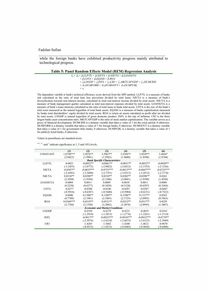
Table 5: Panel Random Effects Model (REM) Regression Analysis λjt = δ0 + β1LLP/TL + β2NII/TA + β3NIE/TA + β4LOANS/TA
+ β5LNTA + β6EQASS + β7ROA
+ ζ8LNGDP + ζ9INFL + ζ10CR3 + ζ11MKTCAP/GDP + ζ12DUMCRIS
+ δ13DUMFORB + δ14DUMGOVT + δ15DUMPUBL
+ εj
The dependent variable is bank's technical efficiency score derived from the MPI method. LLP/TL is a measure of banks risk calculated as the ratio of total loan loss provisions divided by total loans. NII/TA is a measure of bank’s
diversification towards non-interest income, calculated as total non-interest income divided by total assets. NIE/TA is a measure of bank management quality calculated as total non-interest expenses divided by total assets. LOANS/TA is a
measure of bank’s loans intensity calculated as the ratio of total loans to bank total assets. LNTA is the size of the bank’s
total asset measured as the natural logarithm of total bank assets. EQASS is a measure of banks capitalization measured by banks total shareholders’ equity divided by total assets. ROA is return on assets calculated as profit after tax divided
by total assets. LNGDP is natural logarithm of gross domestic product. INFL is the rate of inflation. CR3 is the three
largest banks asset concentration ratio. MKTCAP/GDP is the ratio of stock market capitalization. The variable serves as a proxy of financial development. DUMCRIS is a dummy variable that takes a value of 1 for the crisis period, 0 otherwise.
DUMFORB is a dummy variable that takes a value of 1 for foreign banks, 0 otherwise. DUMGOVT is a dummy variable
that takes a value of 1 for government links banks, 0 otherwise. DUMPUBL is a dummy variable that takes a value of 1 for publicly listed banks, 0 otherwise.
Values in parentheses are standard errors. ***, **, and * indicate significance at 1, 5 and 10% levels.
(1) (2) (3) (4) (5) (6)
CONSTANT 1.0750*** (5.0423)
3.5076** (1.9901)
3.5967** (1.9582)
3.5394** (1.9680)
3.4539** (1.9548)
3.4656* (1.8744)
Bank Specific Characteristics
LLP/TL -0.0021 (-1.2433)
-0.0052** (-2.0772)
-0.0061** (-2.0022)
-0.0051** (-2.0212)
-0.0052** (-2.1353)
-0.0050** (-2.1226)
NII/TA -0.0587**
(-2.4583)
-0.0835***
(-3.3690)
-0.0753***
(-2.7351)
-0.0813***
(-3.0313)
-0.0847***
(-3.4512)
-0.0725***
(-2.7174)
NIE/TA 0.0318**
(2.3058)
0.0298**
(1.9394)
0.0310**
(2.1288)
0.0302**
(2.0041)
0.0298**
(1.9390)
0.0261
(1.4550)
LOANS/TA 0.0004
(0.2238)
0.0011
(0.6277)
0.0005
(0.3429)
0.0010
(0.5128)
0.0011
(0.6297)
0.0005
(0.3264)
LNTA -0.0277 (-0.5916)
-0.0300 (-0.6387)
-0.0240 (-0.5440)
-0.0287 (-0.5984)
-0.0307 (-0.6231)
-0.0447 (-0.7522)
EQASS 0.0690
(0.7788)
0.1300**
(2.1981)
0.1289**
(2.1883)
0.1298**
(2.1725)
0.1317**
(2.0992)
0.0363
(0.7663)
ROA 0.0344***
(2.7704)
0.0319**
(2.1520)
0.0331**
(2.2882)
0.0323**
(2.2078)
0.0317**
(2.0945)
0.0259
(1.3887)
Economic and Market Conditions
LNGDP -0.4194
(-1.2919)
-0.4279
(-1.2813)
-0.4231
(-1.2776)
-0.4035
(-1.2261)
-0.4341
(-1.2714)
INFL -0.0917**
(-2.5974)
-0.0925***
(-2.6218)
-0.0910***
(-2.6075)
-0.0932***
(-2.6123)
-0.0779**
(-2.3049)
CR3 -1.4285 (-0.9515)
-1.5602 (-1.0233)
-1.4200 (-0.9485)
-1.4612 (-0.9826)
-0.9670 (-0.6900)

Financial Repression, Liberalization and Bank Total Factor Productivity…………….
_____________________________________________________________________
MKTCAP/GDP 0.0112*** (2.9407)
0.0113*** (2.9149)
0.0112*** (2.9230)
0.0112*** (2.9276)
0.0108*** (2.9314)
DUMCRIS 0.0727 (1.0521)
Bank Ownership DUMFORB -0.0257
(-0.6030)
DUMGOVT -0.0028 (-0.2391)
DUMPUBL 0.0360
(1.4286) No. of Obs. 154 154 154 154 154 154
R2 0.1175 0.3724 0.3764 0.3729 0.3726 0.4500 Adj. R2 0.0752 0.3238 0.3233 0.3195 0.3192 0.4032
D-W Statistics 1.5127 1.9607 1.9302 1.9583 1.9632 1.8602
F-Statistics 2.7781*** 7.6613*** 7.0923*** 6.9865*** 6.9771*** 9.6147***
The panel regression analysis results indicate that most of the contextual
variables have statistically significant impact on the productivity of Thailand banks.
The empirical findings suggest that credit risk has negative impact on Thailand
banks’ total factor productivity levels. Likewise, the more diversified Thailand banks
tend to be less productive. During the period under study, the findings indicate that
overhead costs exert positive impact on the level of productivity of Thailand banks.
The results also suggest that the relatively better capitalized Thailand banks tend to
be more productive. Furthermore, banks that are more profitable also tend to be
relatively productive.
Business cycle effects, display mixed impacts on bank total factor
productivity. On the one hand, the results support the argument of the association
between economic growth and the performance of the banking sector. On the other
hand, the inflation has negatively impact on Thailand banks’ total factor productivity
indicating that the level of inflation is not fully anticipated by banks in Thailand. The
impact of stock market capitalization is always positive, implying that the Thailand
stock market serves as a complement rather than a substitute to borrowers in
Thailand. During the period under study, the industry concentration of the national
banking system has no significant impact. Similarly, the empirical findings seem to
suggest that the influence of the recent global financial crisis is not significant on
Thailand banks’ total factor productivity.
The results from the panel regression analysis seem to suggest that there is no
significant advantage accruing the foreign owned banks, while the government
owned banks do not appear to be more productive. During the period under study, the
results seem to indicate that there is no impact of stock exchange listings on Thailand
banks’ total factor productivity, implying that the Thailand capital market exerts no
discipline over bank management.
The empirical findings from this study encompass considerable policy
relevance. Firstly, in view of the increasing competition resulting from the more
liberalized banking sector, the continued success of the Thailand banking sector

Fadzlan Sufian
____________________________________________________________________
depends on its productivity, efficiency, and competitiveness. Therefore, bank
managements as well as the policymakers will be more inclined to find ways to
obtain the optimal utilization of capacities as well as making the best use of their
resources, so that these resources are not wasted during the production of banking
products and services. Thus, the policy direction will be directed towards enhancing
the resilience, efficiency, and productivity of the banking sector with the aim of
intensifying the robustness and stability of the financial system.
Secondly, the empirical findings from this study clearly suggest that scale
efficiency has greater influence than pure technical efficiency in the domestic
determining banks’ efficiency levels. If anything could be delved, the small banks
with its limited capabilities could well be at disadvantage compared to their large
bank peers in terms of technological advancements. Therefore, from the policy
making perspective, mergers, particularly among the small banking groups should be
encouraged. This could entail the small banking groups to reap the benefits of
economies of scale. The relatively larger institutions will also have better capability
to invest in the state of the art technologies, which could further enhance the rate of
total factor productivity growth of the Thailand banking sector. Moreover,
consolidation among the small banking groups may also enable them to better
withstand macroeconomic shocks like the Asian financial crisis.
Finally, the empirical findings from this study clearly bring forth the
importance of technological change in determining the domestic and foreign banks’
total factor productivity. The empirical findings from this study clearly demonstrate
the superiority of the foreign owned banks in terms of technological advancements,
which have generally overcome the home field advantage of the domestic banks.
Therefore, constant technological upgrades and investments in the state of the art
technologies should be an essential policy, particularly among the domestic banks in
order to improve the rate of total factor productivity growth of the Thailand banking
sector.
REFERENCES
[1] Banker, R.D. and Natarajan, R. (2008), Evaluating Contextual Variables
Affecting Productivity Using Data Envelopment Analysis, Operations Research 56
(1), 48-58;
[2] Banker, R.D., Charnes, A. and Cooper, W.W. (1984), Some Models for
Estimating Technical and Scale Inefficiencies in Data Envelopment Analysis, Management Science 30 (9), 1078-1092;
[3] Benston, G.J. (1965), Branch Banking and Economies of Scale, Journal of
Finance 20 (2), 312-331;

Financial Repression, Liberalization and Bank Total Factor Productivity…………….
_____________________________________________________________________
[4] Berger, A.N. (2007), International Comparisons of Banking Efficiency,
Financial Markets, Institutions and Instruments 16 (3), 119–144;
[5] Berger, A.N. and Humphrey, D.B. (1997), Efficiency of Financial Institutions:
International Survey and Directions for Future Research, European Journal of
Operational Research 98 (2), 175-212;
[6] Caves, D.W., Christensen, L.R. and Diewert, W.E. (1982), The Economic
Theory of Index Numbers and the Measurement of Input, Output and Productivity, Econometrica 50 (6), 1393-1414;
[7] Chang, H. Choy, H.L., Cooper, W.W., Parker, B.R. and Ruefli, T.W. (2009),
Using Malmquist Indexes to Measure Changes in the Productivity and Efficiency of US Accounting Firms Before and After the Sarbanes–Oxley Act, Omega, 37 (5),
951-960;
[8] Charnes, A., Cooper, W.W. and Rhodes, E. (1978), Measuring the Efficiency of
Decision Making Units, European Journal of Operational Research 2 (6), 429-444;
[9] Charnes, A., Cooper, W.W. and Sueyoshi,T. (1988), A Goal
Programming/Constrained Regression Version of the Bell System Breakup, Management Science 34 (1), 1-26;
[10] Cooper, W.W., Seiford, L.M. and Tone, K. (2006), Introduction to Data
Envelopment Analysis. New York: Springer Science and Business Media, Inc;
[11] Cummins, J. D., Weiss, M.A. and Zi, H. (1999), Organizational Form and
Efficiency: The Coexistence of Stock and Mutual Property Liability Insurers, Management Science 45 (9), 1254-1259;
[12] Evans, D. and Heckman, J. (1988), Natural Monopoly and the Bell System:
Response to Charnes, Cooper and Sueyoshi, Management Science 34 (1), 27-38;
[13] Fare, R., Grosskopf, S., Norris, M. and Zhang, Z. (1994), Productivity
Growth, Technical Progress and Efficiency Change in Industrialized Countries, The American Economic Review 84 (1), 66-83;
[14] Fisher, I. (1922), The Making of Index Numbers. Boston: Houghton-Muflin;
[15] Golin, J. (2001), The Bank Credit Analysis Handbook: A Guide for Analysts,
Bankers and Investors. New York: John Wiley and Sons;
[16] Gregoriou, G.N. and Zhu, J. (2005), Evaluating Hedge Funds and CTA
Performance: Data Envelopment Analysis Approach. New York: John Wiley and
Sons;
[17] Grifell–Tatje, E. and Lovell, C.A.K. (1996), Deregulation and Productivity
Decline: The Case of Spanish Savings Banks, European Economic Review 40 (6),
1281-1303;
[18] Hauner, D. (2005), Explaining Efficiency Differences Among Large German
and Austrian Banks, Applied Economics 37 (9), 969-980;
[19] Isik, I. and Hassan, M.K. (2002), Technical, Scale and Allocative Efficiencies
of Turkish Banking Industry, Journal of Banking and Finance 26 (4), 719-766;

Fadzlan Sufian
____________________________________________________________________
[20] Leightner, J.E. and Lovell, C.A.K. (1998), The Impact of Financial
Liberalization on the Performance of Thai Banks, Journal of Economics and
Business 50 (2), 115-131;
[21] Malmquist, S. (1953), Index Numbers and Indifference Curves, Trabajos de
Estadistica 4, 209-242;
[22] McDonald, J. (2009), Using Least Squares and Tobit in Second Stage DEA
Efficiency Analyses, European Journal of Operational Research 197 (2), 792-798;
[23] Molyneux, P. and Thornton, J. (1992), Determinants of European Bank
Profitability: A Note, Journal of Banking and Finance 16 (6), 1173-1178;
[24] Pasiouras, F. (2008), Estimating the Technical and Scale Efficiency of Greek
Commercial Banks: The Impact of Credit Risk, Off-Balance Sheet Activities, and International Operations, Research in International Business and Finance 22 (3),
301-318;
[25] Pasiouras, F. and Kosmidou, K. (2007), Factors Influencing the Profitability
of Domestic and Foreign Commercial Banks in the European Union, Research in
International Business and Finance 21 (2), 222-237;
[26] Rajan, R.G and Zingales, L. (1998), Financial Dependence and Growth,
American Economic Review 88 (3), 559-586;
[27] Sathye, M. (2001), X-Efficiency in Australian Banking: An Empirical
Investigation, Journal of Banking and Finance, 25 (3), 613-30;
[28] Sealey, C.W. and Lindley, J.T. (1977), Inputs, Outputs and a Theory of
Production and Cost at Depository Financial Institutions, Journal of Finance 32 (4),
1251-1266;
[29] Shephard, R.W. (1970), Theory of Cost and Production Functions. Princeton:
Princeton University Press;
[30] Stiroh, K.J. (2006), New Evidence on the Determinants of Bank Risk, Journal
of Financial Services Research 30 (3), 237-263;
[31] Sufian, F. (2009), Determinants of Bank Efficiency During Unstable
Macroeconomic Environment: Empirical Evidence from Malaysia, Research in
International Business and Finance 23 (1), 54-77;
[32] Tornqvist, L. (1936), The Bank of Finland’s Consumption Price Index, Bank
of Finland Monthly Bulletin 10, 1-8;
[33] White, H.J. (1980), A Heteroskedasticity-Consistent Covariance Matrix
Estimator and a Direct Test for Heteroskedasticity, Econometrica 48 (4), 817-838;
[34] Williams, J. and Intrachote, T. (2003), Financial Liberalization and Profit
Efficiency in the Thai Banking System, 1990-1997: The Case of the Domestic and Foreign Banks,” Working Paper, University of Wales, Bangor.