Redefining Resource Allocation in Computing Systems

Jacob Alan Chasan

Professor Michelle P. Connolly, Thesis Advisor Professor Benjamin C. Lee, Faculty Advisor

Professor Atila Abdulkadiroglu, Faculty Advisor

Honors Thesis submitted in partial fulfillment of the requirements for Graduation with Distinction in Economics and Graduation with Distinction in Computer Science in Trinity College of Duke University.

Duke University Durham, North Carolina

2019

2

Acknowledgements

I am thankful for the inter-disciplinary nature of research at Duke. This thesis connects economic

principles to computer science in an applied fashion, and I am grateful for the support of both the

Economics and Computer Science departments’ willingness to accept this endeavor. I am thankful that

Professor Benjamin Lee was willing to guide me though this research process even when he was on

paternity leave and thankful for Professor Atı̇la Abdulkadı̇roğlu for his insight into auctions and game

theory. Furthermore, I would like to specifically thank Prof. Michelle Connolly for providing valuable

knowledge necessary to create the model and feedback throughout the process of creating this deliverable.

I would also like to thank my thesis seminar fellows, both in the classes of 2019 and 2020.

3

Abstract

A new kernel1 is in town. The current industry-standard for resource allocation on computers does

not take the user’s preferences into account, rather programs are given access to resources based on the

time that each requested to be run. Although this system can lead to solutions that minimize the time it

takes for a program to receive an allocation, it often leads to an incentive misalignment between the

programs and the user. This misalignment is exacerbated as the current queue-based systems have no

inherent mechanism to prevent a tragedy of the commons issue, whereby programs take more resources

from the system than the value they provide to the user. By shifting to a market-based approach, where

computing resources are allocated to programs based on how much utility the user receives from each

program, the incentives of the programs and the users align. With inherent market mechanisms to keep

the incentives aligned, this new paradigm leads to at least superior levels of utility for a user.

JEL classification: C80

Keywords: Auction Theory, Auctions, Markets, Computing, Computer Science, Computing Systems,

Resource Allocation, Technology, VCG Auctions

1 As described in subsequent parts of this paper, the kernel is the core program within an operating system which is

given the authority to allocate the hardware resources amongst the programs on the computer.

4

Table of Contents

I. Introduction ................................................................................................................................ 6

II. Literature Review .................................................................................................................... 11

III. Theoretical Framework ......................................................................................................... 20

VII. Hypothetical System Resource Allocation ........................................................................... 28

VIII. Conclusion .......................................................................................................................... 29

Extension for Multiple Resources ...................................................................................................................... 33

Appendix I. Experimental Framework ....................................................................................... 35

Hardware Component ......................................................................................................................................... 35

Software Component .......................................................................................................................................... 36

Cryptography Workloads ................................................................................................................................... 37

Integer Workloads .............................................................................................................................................. 38

Floating Point Workloads ................................................................................................................................... 38

Appendix II: Data ........................................................................................................................ 40

Appendix IV: Individual Workloads ........................................................................................... 44

Cryptography Workload: AES-XTS .................................................................................................................. 44

Integer Workload: Text Compression ................................................................................................................ 46

Integer Workload: Image Compression .............................................................................................................. 48

Integer Workload: Navigation ............................................................................................................................ 50

Integer Workload: HTML5 ................................................................................................................................ 52

Integer Workload: SQLite .................................................................................................................................. 54

Integer Workload: PDF Rendering ..................................................................................................................... 56

Integer Workload: Text Rendering ..................................................................................................................... 58

Integer Workload: Clang .................................................................................................................................... 60

5

Integer Workload: Camera ................................................................................................................................. 62

Floating Point Workload: N-Body Physics ........................................................................................................ 64

Floating Point Workload: Rigid Body Physics .................................................................................................. 66

Floating Point Workload: Gaussian Blur ........................................................................................................... 68

Floating Point Workload: Face Detection .......................................................................................................... 70

Floating Point Workload: Horizon Detection ..................................................................................................... 72

Floating Point Workload: Image Inpainting ....................................................................................................... 74

Floating Point Workload: HDR .......................................................................................................................... 76

Floating Point Workload: Ray Tracing .............................................................................................................. 78

Floating Point Workload: Structure from Motion .............................................................................................. 80

Floating Point Workload: Speech Recognition .................................................................................................. 82

Floating Point Workload: Machine Learning ..................................................................................................... 84

References .................................................................................................................................... 86

6

I. Introduction

Before presenting the processes by which resources are allocated in a computer, it is important to

have an understanding of how the crucial components of a computer interact with each other. The

hardware of the computer refers to the physical components2 of the computer that are fixed during the

machine’s normal operations whereas the software of a computer refers to the programs that are able to

utilize the physical resources of the computer’s hardware. The software platform which facilitates the

running of end-user programs on the machine is known as the operating system, which is controlled by a

master program known as the kernel. The kernel can be thought of as the benevolent dictator of the

machine as it is given the highest level of control of any program on the machine: it allocates resources,

starts programs, and stops programs.

Each software package is designed to perform a certain set of tasks, which cause different strains

on the hardware system. Before one can understand the new model, one must first understand current

methods of resource management within computing systems. The operating system’s kernel runs the

scheduling algorithm, which orders when programs are able to access the machine’s resources. Although

the kernel technically has the power to allocate the machine’s resources, it does not utilize an economic

model to efficiently distribute the allocations, rather it relies on temporally-based scheduling algorithms

to decide which process can be scheduled for execution before another, often times leading to inefficient

resource allocations from the perspective of user utility.

A consistent goal within the technology industry has been to increase the utility a user derives

through use of a system by providing better, faster, and less expensive solutions. Staying true to this age-

old goal, this thesis develops and tests a software system that is theoretically implementable on existing

2 Examples of hardware components could be the Central Processing Unit (CPU), Random Access Memory (RAM),

or a hard drive.

7

hardware systems that gives a user superior utility to that derived from existing platforms. In such a

system, the Kernel would take an active role in managing the resources.3

The following example illustrates the current issue from an end user’s perspective. Suppose you

are writing a document in Microsoft Word on a battery-powered laptop while browsing the internet in

Google Chrome. Your utility gained by you is primarily based on the speed by which you are able to

complete your task of writing the document. Possible bottlenecks occur where the computer is not

responding in a reasonable time to your input or is not able to execute its task. Although you may only see

the apps Microsoft Word and Google Chrome open, hundreds of programs are running in the background,

competing for and consuming the same resources as the programs that you are actually engaged with, but

are not providing you the same level of utility.

For example, consider the Photos app. Off-screen, this app runs Machine Learning “ML”

algorithms on your photos and videos to provide you with insights on who is in your photos and collections

of photos that are likely related. At the moment, you simply wish to write your document and access the

internet–the Photos image processing provides you little-to-no utility.

In your current state, your utility would be maximized if your computer allocated its resources

towards the task you are trying to complete: writing a word document and browsing the internet. Instead,

however, the computer will simply allocate the resources to whichever program is first in the list of

programs to be given resources based on the time that the program requested the resource from the Kernel.

So, instead of your laptop’s battery lasting the entire day and Microsoft Word quickly reacting to your

3 Systems are divided into two classifications: single and multiple units. A single-unit is a complete machine which

does not rely on or utilize the computational resources of other machines. A multiple-unit cluster is a system of several machines addressable as one. A multiple-unit cluster does not have one Kernel, as each unit within the cluster has its own Kernel. Instead these large machines have governing software–akin to super Kernels–which instructs each Kernel on what it should do. For cluster-based systems, this resource allocation would live in the cluster controller software. Regardless of the type of machine, each has a similar premise.

8

clicks, your laptop is burning through its battery scanning your photo library without you even knowing

and Microsoft Word is not responding.4 In this scenario, your utility is diminished.

Under a more market-based resource allocation, the user would receive a higher level of utility.

Instead of the Kernel allocating resources based on a list of whichever programs requested resources first

without taking the user’s preferences into account, it would allow each program to “bid” for resources.

Programs giving the user the most utility would win access to the resources they need to fully function,

and programs providing little utility would lose access to the resources until such a time as the “cost” of

the resources decreases. Continuing with the previous example, the Photos app would not have the

“money” to buy the resources necessary to scan your photo library due to the high price of resources given

the battery power and other resources needed to provide the highest level of utility to the user for your

current document writing task. Your battery would now be saved for use by Microsoft Word and Google

Chrome and these programs would respond to your input faster.

The tragedy of the commons issue–whereby programs overuse the resources available in the

machine–is recognized in industry, but current solutions rely on an “observer” approach.5 The kernel sends

each program a notification when the computer enters or exists a pre-defined binary device state–e.g. Low

Power Mode and Low Data Mode. It is up to a software developer how–and even if–their program should

change its configuration based on these modes. As the form factors of computers have changed–from

mainframe to desktop to laptop to smartphone–the various modes available have increased in number. It

can be very costly for a developer to implement compliance for each of the modes, and thus it is not in

their incentive to write their program in a such a way as to always adhere to the configurations of the

device’s modes. Furthermore, the kernel does not provide the program with levels as to the user’s

4 A more technical definition would refer to this as a program “hang” whereby the program is currently stalled awaiting

resources on the machine to free up. 5 See Apple Developer https://developer.apple.com/library/archive/documentation/Performance/Conceptual/ EnergyGuide-iOS/LowPowerMode.html

9

preferences, rather it only provides a binary result of whether the mode is activated or not (e.g. “user

requests programs to reduce power usage” or “user is not concerned with power usage”).

A market-based approach would align the incentives of the program and those of the user. Each

program would be held in compliance with the user’s preferences by the market for system resource

allocation and be able to respond to every state of the machine, not just those which have been pre-

programmed (e.g. the power or data states mentioned above). On the supply-side of the market, although

the computer system has a fixed supply of resources, the amount of free and allocable resources is

constantly in flux. On the demand-side of the market changes with similar frequency as user preferences

can change and programs may need a different allocation of resources to complete the task at hand. The

changes made on both the supply and demand sides of the market can be seen as individual events, and as

such, the kernel can run the market allocation system again when such an event occurs. As this system is

optimizing for user utility using a market, this paper shows how such a system results in a superior level

of utility for the user.

Before proceeding, it is important to note a simplification that follows through this paper. Instead

of considering multi-resource bundles, this paper considers only single resource auctions as this greatly

reduces the complexity of the problem at hand and allows the model to be illustrated through experimental

data.

Often, programs rely on multiple resources from the computer to complete their tasks. Take a

videoconferencing application (e.g. FaceTime, Skype, Cisco WebEx) as an example. As its primary

functionality is facilitating multi-way video and audio communications, the software requires an internet

connection to send and receive files, a camera processing system to capture images, and a media encoding

/ decoding system to convert the files to and from a transportable format. This means that the system will

require the use of certain resources (e.g. CPU, GPU, RAM, network bandwidth, camera, etc.) to function.

10

Constructing an auction that would allow for bids of these multiple resources would create a surface which

has one dimension for every additional resource that is part of the bundle, which then would be analyzed

to find the allocation most optimal to the user, given their current set of priorities. For the purposes of this

paper, package bidding is expressly disallowed within the resource auctions for sake of simplicity; thus,

the model proposed herein represents a 2-dimensional slice of the multi-resource model.

11

II. Literature Review

II. A. Traditional scheduling algorithms

The new resource allocation system defined in this paper would take the place of the current

temporal-based approaches, and as such, one must understand the benefits and drawbacks to the industry

best-practices. The major algorithms used today do not optimize the user’s utility, rather they either

“maximize CPU utilization under constraint that the maximum response time is 1 second”6 or maximize

“throughput such that turnaround time is (on average) linearly proportional to total execution time.”7

Silberschatz (2008) has written about the common algorithms in Operating System Concepts, where he

identifies the six major resource scheduling algorithms.8 Each is explained in turn.

The most basic scheduling algorithm used in industry is the First-Come-First-Serve Scheduler9.

This algorithm consists of a queue of programs waiting to be executed, which can be thought of as a list

first-in-first-out list. An individual program advances its position in the queue when the current program

that is using the computer’s resources has finished executing. The main downside to this algorithm is

known as the “convoy effect,” whereby a bottleneck in the advancement of every process can occur should

the process being executed is complex and takes a long time to finish. An analogy to this algorithm is a

sandwich deli counter. Customers form a line and, although each is processed one-by-one, the previous

customer does not have to be completely finished before the next one begins to be served. A bottleneck

6 Operating System Concepts 213. 7 Operating System Concepts 213. 8 A more comprehensive understanding of how these algorithms work require a study of the four states of programs:

Running, Ready, Waiting, Terminated. A process is said to be running if it is currently being executed by the physical CPU. A program that is the next-to-run is said to be in the Ready state. Programs that are not “on-deck” are said to be waiting to be ready. Programs that are neither loaded into memory nor running on the CPU are considered terminated as they are effectively switched off.

9 Operating System Concepts 188.

12

occurs when one person in the line either makes a complicated sandwich or is indecisive about which

sandwich they are ordering.

Two variations of the First-Come-First-Serve algorithm are used in practice, known as Round-

Robin and Multilevel Queue. The Round-Robin Scheduling10 method assigns a timer to switch between

processes every so often, preventing the issue of one process from clogging the queue. Multilevel Queue

Scheduling11 extends the original algorithm by creating additional queues, each with different priority

levels. Once a program is designated to a certain priority queue, its priority queue cannot be changed until

the program has been executed. Multilevel Feedback Queue Scheduling12 is a variation the algorithm

which allows for the priority of the program to be changed after it has been first assigned. Two common

flavors of this system exist. In the first, all programs scheduled in the highest priority queue must be

completed before the next level of queue is started, which can cause the problem of low priority queues

never being addressed. In the second, the processor’s resources are split over the different levels of the

queues, giving most of the processor resource to the highest queue, and smaller allocations to queues with

lower priority.

The main drawbacks to the previous algorithms are that they do not include a program-specific

priority. Programs are either run in the order they are submitted to the processor or run based on their

bucket. Should a program need to be given immediate priority, these algorithms provide no path by which

to change the order in the queue. Priority Scheduling13 is a different approach to the simple queue

algorithm which attempts to solve this issue. Each program is assigned a priority, and the priority level

sets the order of which program is selected to run the next time resources become available. Generally,

priorities are a continuous integer range, where smaller numbers represent higher priority. The most basic

10 Operating System Concepts 194. 11 Operating System Concepts 196. 12 Operating System Concepts 198. 13 Operating System Concepts 192.

13

form of this scheduling system suffers from a pitfall where new high-priority programs are added to the

queue before it ever finishes processing the lower priority programs, leading some low priority programs

never being allocated any resources to execute. The workaround in practice has been to increase the

priority of all programs in the queue either when one finishes or when a designated time interval has

passed.

One alternative to the First-Come-First-Serve set of algorithms is known as the Shortest-Job-

First Scheduling.14 This final algorithm is used to determine the priority of when programs should run.

Unlike the previous algorithms, which prioritized the running of the programs in a queue, this algorithm

optimizes which programs are bound to run in the shortest amount of time, and thus consume the least

processor resources. By running the programs from a shortest-time to longest-time perspective, the system

is able to reduce the average wait time for a program. The downside to this approach is that programs

considered to have a high priority that are not the least complex program will see a delay in their execution.

Such delays can decrease the user utility as the user’s priority is not being taken into account.

To address this issue, “virtualized” environments are created, where a systems engineer can set

resource constraints for a complete operating system which runs on top of the existing computer and

operating system. By setting these constraints on the virtual system level, the kernel in charge of the virtual

environment cannot see any additional resources and is prevented from abusing the system resources by

participating in a tragedy of the commons beyond the set resource limits. Although this virtualization

system does help alleviate the resource abuse problem, it requires a great amount of computing overhead

to achieve as another kernel, and all the related system management programs, must be used in each virtual

computing instance. Although this can help move the performance of the computer closer to that which

14 Operating System Concepts 189

14

would provide the user the most utility, it still is not a system which optimizes directly for the utility that

the user derives from use.

II.B. Market-based scheduling

One way to create a system to optimize for the user utility is to allocate the resources of the system

using a market-based approach. Kuwabara (1995) presents an early picture of how a system could better

allocate resources to optimize for the utility of each program. The paper puts forth the critical idea of an

information barrier between the parties involved in the transaction, which as discussed later leads to

incentive alignment between the programs and the user as well as added security within the system. The

major drawback to the approach taken by Kuwabara is that instead of making the price “determined

through bidding,…the resource prices are determined by their associated seller based on the demand for

the resource” thus eliminating “the overhead associated with the bidding process.15 When thinking about

the stakeholders in a computer system, the most important is the user. Optimizing for the utility of each

program can lead to the programs having a better outcome, but if these programs are not highly valued by

the user, the outcome will not give the user–who ultimately controls the computer and its processes–the

highest level of utility.

In order to optimize for user utility, one must first define metrics that differentiate the utility that

the user derives from execution of the programs on the machine from that of the programs themselves.

Chun16 (2002) defines “user-centric performance metrics” which are used to “focus on user value as

opposed to system-centric metrics which do not take utility into account and thus are not good measures

of how satisfied users are with their resource allocations.”17 Although the paper utilizes an auction to

15 Kuwabara 2. 16 The Chun paper does provide a thorough explanation of an experimental framework that can simulate and test the

scheduling algorithms, which is extended and used in this paper. 17 Chun 1.

15

power the market mechanism, it does not explain how the overhead issue mentioned in Kuwabara is

overcome, rather simply concluding that the solution “delivers up to 2.5x higher performance” in

comparison to the standard First-In-First-Out scheduling algorithm defined earlier in this section.

Once one understands how to define user utility, the next step is to understand how to align the

allocation of program resources such that they are in-line with the user’s preferences. In a set of papers

from 2014 through 2018, Zahedi and Lee begin to find the efficient resource allocation given a specific

piece of software, especially in environments where multiple programs had to share common resources.

Once the optimal allocations were measured, the papers determine an economic model to relate the user

utility to the allocation of resources for a given program. The final piece is adding tokenization to resources

so that a price can be assigned to a scarce resource. This allows for the process of resource allocation to

be inherently forward-looking as the optimal allocations for a program are known a priori, programs are

able to bid for their share in a low-cost manner. In their model, the resource allocation system is thought

of as a game with multiple sequential rounds of bidding. As such, they also model the impact of the cost

of running the auction against the gains made by the allocations seen from the market-based system.

Although this method outperforms the queue-based mechanisms described earlier by a sizable amount, its

market-based mechanism does not rely on the program-level. In order to truly optimize the utility of the

end user, each program must make the resource allocation decision about type and quantity.

Zahadi (2018) extends this work by exploring differing functions that can be used to represent the

optimal resource allocation with relation to the user’s utility. The additional insight shows that although a

standard Cobb-Douglass function inherently contains few assumptions about convexity, a Leontief

function, which is more convex and monotone in comparison, can better explain the optimal resource

allocations when combined with Amdahl’s law.18 Although this thesis does not focus on the specific

18 Amdahl’s law is an argument and related expressions that explains how the execution time of programs will improve

should the resources allocated to the program by the system increase.

16

function that models user utility, it is important to understand the contenders and that it is possible to

construct a market-based tokenization mechanism for distributing resources that is able to be run

dynamically when the user utility preference function changes.

II. C. Auction Theory

The key points to consider when selecting the market mechanism for this resource allocation

system is superior utility to the user and low overhead cost.

Although the auctions Kuwabara analyzed in 1995 were cost prohibitive, a sealed-bid mechanism

can be applied to this problem with low overhead cost of execution. In traditional open-bid auctions,

frictions exist because once the auctioneer has called out a price, every participant knows the current

highest-bid and is allowed a certain amount of time to think about whether they would like to place a

higher bid. When there are many bidders and many items, this process can take a significant amount of

time and does not provide the incentives necessary to force each bidder to reveal their true maximum

willingness to pay.

Should a mechanism exist to that incentivizes the bidder to reveal their true value of the item, as

it is in the incentive for each bidder to maximize its profit, a first-price auction will lead to a profit of $0.

Should a participant bid more than their true value then the bid can only lead to a worse outcome. In a

second-price sealed-bid auction, the profits made are the difference between the highest bidder’s true value

and the second highest bid, giving the ability to earn positive profits.

Vickrey (1961) presents one of the first auctions that meets the criteria of both second-price and

sealed bid. His proposal has four distinctly different features from the Dutch auction: 1) it is designed to

naturally give bidders the incentive to reveal their true maximum price to the auctioneer and establish a

17

Nash equilibrium for the parties involved;19 2) participants submit sealed bids at one time preventing each

from knowing the other’s bid; 3) the auctioneer does not have to call out prices, rather they can make the

winner decision from the already submitted-bids; 4) the winning bidder would pay the second-highest

price. This type of auction subsequently became known as a “second-price sealed-bid” process. Vickrey

identified two weaknesses to his auction type that are addressed in subsequent papers: high cost of multiple

rounds of bidding and reliance on an honest auctioneer. As the auction is designed to force every bidder

into revealing their maximum willingness to pay, in its basic form, it should not require multiple rounds

of bidding. Should the items up for auction become greater than one or the predefined quantity change, it

would be costly as the entire procedure of sealed bids would have to be run again. The second drawback

is related to the auctioneer: in a standard or Dutch auction, as the auctioneer calls out the bids, there is no

way for fraud to occur on the part of the auctioneer but in this case a crooked auctioneer could not select

the highest-bidder as the winner. As the kernel is the auctioneer in the case of system resource allocation,

it can be assumed that it is honest.

Edelman, Ostrovsky, and Schwartz (2005) present a model for how an extended version of the

Vickrey auction–known as the VCG system after contributions by Clarke (1971) and Groves (1973)–can

be run with a bidding function instead of the participants sending a single static price bid to the auctioneer.

As each bidder can make offers on varying amounts of the resource in question, it is important that the

bidder be able to submit a single “bid” to the auctioneer from which the winning price and quantity can

be determined in a single round, thus leading to low execution frictions and costs. Edelman’s work

surrounded the market for internet advertising auctions, whereby a bidder can submit a complex pricing

formula requiring several inputs as their bid without knowing exactly what goods were available to bid

on, rather knowing what quantity and ratio of items could be available for auction at any moment

19 Described in more detail in: “Algorithmic Game Theory” by Nisan, Roughgarden, Tardos, and Vazirani.

18

The auctioneer program would then run each bidding function to determine each bidder’s

willingness to pay in that instance. After ranking the bidders by price, the bidder whose function produced

the highest value is declared the winner and pays the amount of the second-highest bidder. As this

computation is done by the automated auctioneer, the auction can proceed at a very rapid pace. Although

bidders are allowed to change their bidding functions in the internet advertising auctions, in order to

remove the incentive for a bidder to learn from their past bidding, one can augment this by only allowing

a bidder to update whether their function is active or inactive. This system can be applied to the market

for system resource allocation with very few modifications.

Although Edelman presents the primary model for internet advertising auctions, the key

considerations for this market are shown in Mahdian, Nazerzadeh, and Saberi (2006). They identify them

as a system that 1) results in an optimal or near optimal allocation of advertisements to resource-conscious

bidders; 2) is capable of computing this solution in a short amount of time and utilizing few resources, as

the “market” conditions only hold for a short period of time; 3) when the bidders have “unreliable

information about the future” and their resource needs at that time; and 4) functions correctly when

unexpected events occur.

The systems framework constructed within this paper shares the same four core tenants: 1) the

user’s desire to achieve the highest level of utility given the resources available to and demands on the

system; 2) the need for the system to make allocation decisions quickly as the needs of the user change

with every user interaction; 3) individual programs can predict the resources necessary to complete their

current tasks, but likely cannot compute the resources necessary to compute tasks that require user

direction;20 and 4) allow the system to quickly respond to a drastic change in priorities of the user without

20 An example being a case where a web browser must wait for the user to tell it which resource to locate from the

internet. Downloading a video file requires more system resources than loading a plain website.

19

prior notice. Due to the shared tenants between these two problems, the literature relating to internet

advertising auctions applies to the problem of system resource allocation as presented in this paper.21

This formula-based approach was only made possible by computer bidding. Prior to the general

availability of the internet and computers, multiple rounds of VCG auctions would require significant

amounts of time. Should a resource change, the auctioneer would need to notify each bidder and collect

revised bids. Before submitting a new offer, the bidder would have to think what their new maximum

willingness to pay would be. Simply said, prior to the information age, the VCG auction required

simplicity to execute, partially dampening its usefulness over other auction types.

The VCG system also has the result of producing an output that is a Nash equilibrium that is envy-

free. Aggarwal, Feldman, and Muthukrishnan (2006) explores the innerworkings of this equilibrium and

the assumptions and conditions necessary for the auction to produce this type of equilibrium. Aggarwal

makes the key definition of an envy-free pricing and allocation model as one where “each bidder prefers

the current outcome (as it applies to her) to being placed in another position and paying the price-per-click

being paid by the current occupant of the position.”22 The paper then further shows that assuming that the

bidders reveal their true valuations, the result of the VCG auction will result in “the most efficient

allocation.”23 The key to this supposition holding is that the situation aligns the incentives of the bidders

to reveal their true valuation to the auctioneer.

With the bidders revealing their true valuation function to the auctioneer, a cost-effective

market can be applied to a computer’s system resource allocation in such a way to optimize for the utility

of the user.

21 One other similarity of note between these two problems is that internet advertising naturally imposes the

assumption that each auction only allows for one resource to be bid for at one time. Although computer programs often require multiple resources to function, as explained later. This paper imposes the condition that each resource auction run by the computer can only offer one resource. This simplifying assumption allows for the results of the model to be validated experimentally.

22 Aggarwal 6. 23 Aggarwal 6.

20

III. Theoretical Framework

Macroeconomic System Model

Before running an auction or allocating resources to the programs, the macroeconomic system

must first be established. The economic framework presented in this paper benefits from the fact that the

macroeconomic environment is a vacuum: we start with a blank slate and are able to impose whatever

constraints necessary in order to make the incentives align between the individual programs, which are

treated as “firms,” and the user. Even though the incentives are aligned, in the case of “bad” programs, as

the kernel has the ultimate power over each program on the computer, the punitive actions assigned for

individual program misbehavior are absolute. Further, we program the kernel to be honest, thus avoiding

any issues relating to a fraudulent auctioneer.24 These constraints are not assumptions, rather they are

incentive compatible rules that are programmed into the kernel that are defined to be followed strictly and

without error. This allows the model to be inherently simpler than those seen in typical macroeconomic

analyses. Furthermore, the timeline of the economy is not driven by hours, minutes, and seconds, rather it

is determined by how often the programs come to the market to get an allocation of resources.

As each program is thought of as a profit-maximizing firm: spending as few units of currency as

possible to get the resource which will generate the program the most revenue, which is defined as the

utility the program provides to the user. Each program stores its funds in a “bank account” provided by

the kernel, where it is able to deposit revenues and draw down from when it acquires resources. An

individual program’s assets can be expressed as follows:

𝐴" = 𝐴$ − 𝐵$ + 𝑈) and more generally, 𝐴*+" = 𝐴* − 𝐵* + 𝑈,

24 Should the kernel not be honest, the computer would not be worth buying from the user’s perspective as the machine

would maximize the kernel’s utility–not that of the user.

21

Where 𝐴, represents the total assets of the program, 𝐵, represents the “bid” price of how much the

program pays for the resource, 𝑈, represents the income received after completing the task.

Side Markets and Collusion

Within the macroeconomy of the computer, one must consider side markets and collusion amongst

the individual programs within the system, as both are likely to occur for economics and computing

reasons that could lead to the failure of the market for resource allocation, leading to lower levels of utility

for the user.

In order to align the incentives of the programs to those of the user, side markets and the

transference of resources to unrelated25 programs must be banned as it may be in the best interest of an

individual program to sell resources it just purchased at auction to another program. The issue with it is

that in these situations, certain private markets are created whereby not all members of the population are

eligible to participate in the auction. Were side markets allowed, monopolistic competition would likely

form as programs from well-known developers would be able to exchange a large enough allocation of

resources amongst themselves that programs by less well-known developers would be unable to purchase

the quantity of resources they need from the kernel, as the kernel would not be able to direct all of the

resources of the machine–only those which are being traded in the “public” resource markets.

The ban on side-markets can be achieved by considering the allocations of resources received at

auction as perishable goods. Note that the computer’s resources are still considered durable goods, only

the actual allocation that a program wins at auction experiences a 100% depreciation immediately after

the auction has concluded.

25 An example of “related” programs would be Microsoft Word and Microsoft Excel, which share a common codebase

and are given a special super-sandbox allowing them to communicate unrestricted with any program in the Microsoft Office Suite, but follow the same standards of communication with any program not part of this software bundle.

22

Collusion also is prevented in this system, as two programs which collude on a bidding strategy

have the ability to “rig” the second-price sealed-bid auction in such a way as to know more information

than other bidders, and thus bid accordingly. As such, if any collusion were possible, the bidder’s

incentives may not align their bid with their true willingness to pay.

The prevention of side markets and collusion also aligns with the interest of computer security.

Modern computing systems enforce a strict policy of application “sandboxing,” wherein individual

programs are prohibited from interacting directly with each other without going through the operating

system’s Kernel. This design paradigm came about due out of computer security concerns. Without

sandboxing, any program is able to read (and in some instances write) the data that is in use with another

program. An example of this would be as follows: suppose you were running two unrelated programs–

Google Chrome (a popular web browser which stores your internet passwords) and Microsoft Outlook (a

popular email client which stores your emails and email password). Google Chrome could inspect the data

of Outlook and read the password and steal the emails, and Outlook could read the internet passwords

from Google Chrome.

With the hundreds to thousands of pieces of software installed on modern consumer machines, it

is not feasible to rely on a “trusted developer” system whereby each developer commits to ensuring the

safety of all other developers’ applications and data. The solution to this problem is to prevent any

unrelated apps from talking to each other directly. Were a side market allowed, apps would be able to

exchange memory without the kernel’s knowledge, and thus violate the individual containerization that

comes with sandboxing, exposing the user to a security vulnerability. By enforcing sandboxing, unrelated

programs are naturally unable to directly communicate with one-another, thus not able to collude with

each other and ensuring that the valuation of resources by each program is independent of other programs

and no market speculation can occur by programs.

23

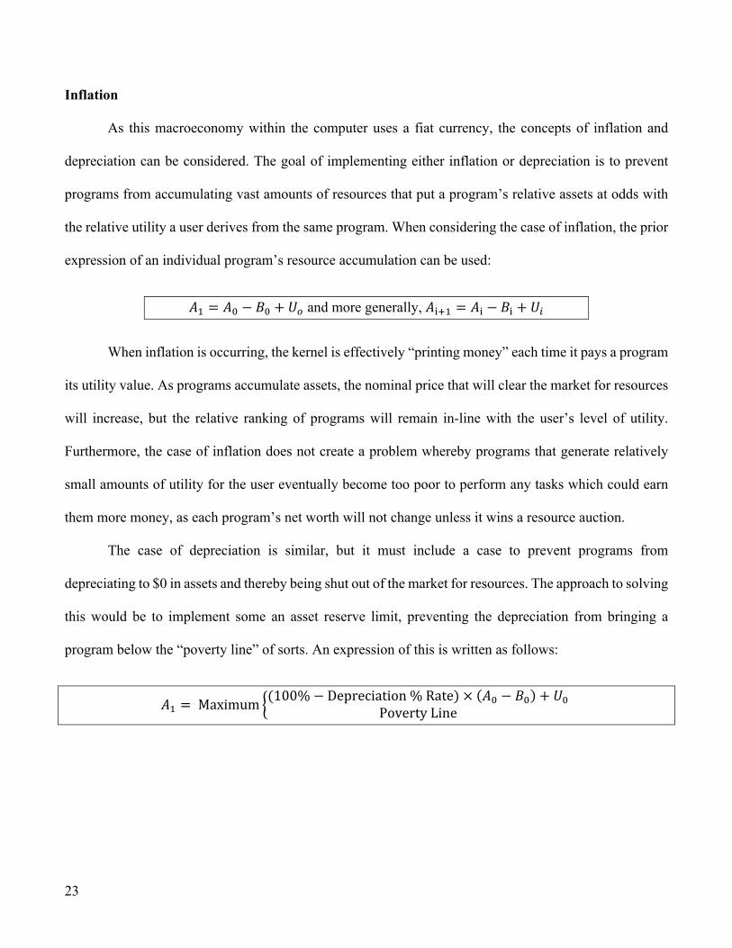
Inflation

As this macroeconomy within the computer uses a fiat currency, the concepts of inflation and

depreciation can be considered. The goal of implementing either inflation or depreciation is to prevent

programs from accumulating vast amounts of resources that put a program’s relative assets at odds with

the relative utility a user derives from the same program. When considering the case of inflation, the prior

expression of an individual program’s resource accumulation can be used:

𝐴" = 𝐴$ − 𝐵$ + 𝑈) and more generally, 𝐴*+" = 𝐴* − 𝐵* + 𝑈,

When inflation is occurring, the kernel is effectively “printing money” each time it pays a program

its utility value. As programs accumulate assets, the nominal price that will clear the market for resources

will increase, but the relative ranking of programs will remain in-line with the user’s level of utility.

Furthermore, the case of inflation does not create a problem whereby programs that generate relatively

small amounts of utility for the user eventually become too poor to perform any tasks which could earn

them more money, as each program’s net worth will not change unless it wins a resource auction.

The case of depreciation is similar, but it must include a case to prevent programs from

depreciating to $0 in assets and thereby being shut out of the market for resources. The approach to solving

this would be to implement some an asset reserve limit, preventing the depreciation from bringing a

program below the “poverty line” of sorts. An expression of this is written as follows:

𝐴" = Maximum 4(100% − Depreciation%Rate) × (𝐴$ − 𝐵$) + 𝑈$PovertyLine

24

User Preferences

As the basis of this entire model is related to achieving a superior level of utility for the user, it is

critical that the system knows what the user’s preferences are and how these preferences translate into

utility.

Determining the user’s true preferences and corresponding utility is a complex problem as the

preferences are greatly influenced by the way the human interacts with the computer. Further, the utility

derived from the program requires a study in behavioral economics as it is not necessarily the case that

the user’s preferences (i.e. what they think they want) is perfectly correlated with the utility gained from

a system configured with those preferences (i.e. what they actually want).

This paper assumes that the user preferences and corresponding utility that is derived from each

program can be found ex ante through market research about the user before the programs are loaded onto

the computer. The reason for this is that this computer would be produced by a profit-maximizing firm

which may want to demonstrate the benefits of the system over a baseline system to show why the system

is “pre-modeled” to the user.

Revenue and Profits

When a program is first loaded onto the computer, it is given an endowment whereby it can enter

the resource allocation market and begin reaping the rewards of utility generation. The best way to create

this allocation would be for the kernel to already have a sense of user preferences and allocate the resources

in a way that is commensurate with the utility generated by the new program relative to that generated by

other programs. Should this data not be available a priori, each new program can receive the average

endowment and, with time, will find its relative ranking amongst the other programs. This occurs because

the more auctions conducted, the more this program will either make additional profits–thereby increasing

25

its relative wealth–or not win the auction–thereby decreasing its relative wealth. The kernel is able to

update the priority of programs based on the frequency and amount of deposits made by each program as

the higher the frequency and amount, the more utility the user gains from the program. In the long-run,

the relative ratios of each program will accurately express the user preferences for each program’s relative

level of utility generation.

When a program completes its task, it receives a paycheck from the kernel in the amount of the

utility it generated for the user, deposited into this account. The winning bidder will receive profits due to

the auction’s design: as a second-price auction, the winning bidder’s willingness to pay is the highest bid

put into the auction, but this bidder only ends up paying the second-highest bid. The profit is the difference

between the amount of utility the program generates and the cost of acquiring the resource:

𝜋IJKLJMN = BidIJKLJMN − 2ndHighestBid

Bidder Learning

Due to the construction of the auction and perishable nature of the asset allocations, there is no

incentive to a bidder learning from the auctions it has participated in the past. Programs must submit their

resource valuation functions at the time of their install but are unable to dynamically change their valuation

program after install.26 Giving the programs the ability to activate or deactivate their function allows the

function to operate under its existing valuation function, but gives no advantage for a program to action

based on information it has learned from the past rounds of auctions.

Note, however, that this is not to say that programs will not learn the habits of the users. Instead,

this states that a program can gain no advantage should they be able to learn from their prior bidding

26 A program is able to update its function if it were to install an update, still preventing the incentive for the program

to learn as the valuation function is defined a priori to the runtime of the program.

26

history as in each auction, it is in the bidder’s best interest to reveal their true valuation function to the

kernel. Furthermore, the kernel has the ability to learn from the user’s habits and adjust the payouts to

reflect the utility a user gains from each individual program.

Incentive Compatibility

Each program has an incentive to reveal its true valuation for resources to the kernel. This incentive

compatibility exists because of the constrained endowment of each individual program, whereby

overbidding would lead to each program purchasing a quantity of resources at a price which would not be

profit maximizing. The programs also have an incentive against underbidding because if a program

submits a bid below its willingness to pay, it may not win the quantity of a resource it needs in order to

complete the task from which the user derives utility and the program gets paid. Because of these upper

and lower incentives, it is in the best interest for the program to reveal its true willingness to pay when

entering the auction.

Kernel Infrastructure Programs

The final constraint necessary for the auction is a reserve of resources for the kernel and its

infrastructure programs. Certain programs (graphics subsystems, keyboard input drivers, etc.) are

subsystems of the kernel and are necessary in order for almost any program to function properly on the

computer. Should these resources be constrained, no matter the allocation given to the end-user programs,

the user will not derive the full value of the utility as these programs will be unable to deliver on their

utility promise. To ensure the computer’s infrastructure always has the resources to function, the kernel

sets aside the resources it needs to provide these support systems, and only auctions the residual resources

to the end-user programs.

27

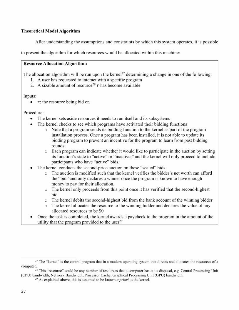
Theoretical Model Algorithm

After understanding the assumptions and constraints by which this system operates, it is possible

to present the algorithm for which resources would be allocated within this machine:

Resource Allocation Algorithm: The allocation algorithm will be run upon the kernel27 determining a change in one of the following:

1. A user has requested to interact with a specific program 2. A sizable amount of resource28 𝑟 has become available

Inputs:

• 𝑟: the resource being bid on Procedure:

• The kernel sets aside resources it needs to run itself and its subsystems • The kernel checks to see which programs have activated their bidding functions

o Note that a program sends its bidding function to the kernel as part of the program installation process. Once a program has been installed, it is not able to update its bidding program to prevent an incentive for the program to learn from past bidding rounds.

o Each program can indicate whether it would like to participate in the auction by setting its function’s state to “active” or “inactive,” and the kernel will only proceed to include participants who have “active” bids.

• The kernel conducts the second-price auction on these “sealed” bids o The auction is modified such that the kernel verifies the bidder’s net worth can afford

the “bid” and only declares a winner once the program is known to have enough money to pay for their allocation.

o The kernel only proceeds from this point once it has verified that the second-highest bid

o The kernel debits the second-highest bid from the bank account of the winning bidder o The kernel allocates the resource to the winning bidder and declares the value of any

allocated resources to be $0 • Once the task is completed, the kernel awards a paycheck to the program in the amount of the

utility that the program provided to the user29

27 The “kernel” is the central program that in a modern operating system that directs and allocates the resources of a

computer. 28 This “resource” could be any number of resources that a computer has at its disposal, e.g. Central Processing Unit

(CPU) bandwidth, Network Bandwidth, Processor Cache, Graphical Processing Unit (GPU) bandwidth. 29 As explained above, this is assumed to be known a priori to the kernel.

28

VII. Hypothetical System Resource Allocation

An example of the theoretical model would be as follows: suppose a computer had four programs

with the following payoffs segmented by operating state:

1. Program A (not in use: $0, in background: $5, in foreground: $50) 2. Program B (not in use: $0, in background: $10, in foreground: $0) 3. Program C (not in use: $0, in background: $5, in foreground: $30) 4. Program D (not in use: $0, in background: $40, in foreground: $80)

Each program initially can start off with an endowment of their foreground payoff, and the kernel

reserves $10 worth of resources to run its infrastructure programs. The kernel has $100 of CPU available,

and after reserving $10 for itself, leaves $90 on the table for allocation. The user desires to open programs

A, B, and C, which in this case would lead to a total demand of $90–exactly equal to the supply available

to allocate. In this case, there would be no resource constraint, and the allocation would occur without

further considerations. The kernel debits the program’s the amount of their willingness to pay and after

successful execution (i.e. after which point the user has derived their utility from the programs), the kernel

will deposit the utility into the programs’ bank accounts.

In a second example, the user desires to open programs A, C, and D while the kernel still has $90

available to allocate. Note that in this case, the total demand is $160, which exceeds the available supply.

As each program has presented the kernel with a bidding function relating to the amount it is willing to

pay given a certain quantity of resource in various states, the relative price of 1 unit of CPU naturally

would increase. The kernel simply runs the bidding function to determine which programs would be

willing to pay the most, concluding that Programs D and A would derive the most from allocations. The

quantity awarded to each program is based on the relative difference in utility that is achieved by that

program (i.e., does 1 additional unit of CPU give the same value of utility to the user in the case of both

programs).

29

VIII. Conclusion

Connecting the experimental data (see Appendices) with the theoretical framework allows for a

real-world simulation of the allocation system for processor cache. Cache relates to a processor as a sticky

note relates to a four-function calculator. At a high level, a computer processor takes data and a simple

function code telling which function to perform on the data as input. In order to perform complex

operations, the processor has to store the output of each calculation so that it can be accessed quickly for

in subsequent execution cycles. Using the data gathered in the experimental portion of this paper allows

one to compare the tradeoff of the time it takes to execute the program against the amount of cache that is

allocated to the processor cores within the computer. Using this data, one can perform a simulation of the

utility outcome of the user, given their preferences and the constraint of cache space on their computer.

Suppose the user has a MacBook Pro30 with 16MB of Level 3 cache that has the following user-

loaded programs that have payoffs as follows:

1. Google Chrome (3MBs, not in use: $0, in background: $10, in foreground: $90) 2. Mail (3MBs, not in use: $0, in background: $10, in foreground: $60) 3. PDF Reader (3MBs, not in use: $0, in background: $0, in foreground: $30) 4. Photos (7 MBs, not in use: $0, in background: $5, in foreground: $20)

The relative speed of each process is shown in the below graphs, comparing the amount of time it

takes the process to run against the megabytes of Level 3 cache allocated to the process:

“Google Chrome” – HTML5:

“Mail” – SQLite:

30 MacBook Pro 15,1 with Retina Display and Touch Bar with a Core i9 Processor

30

“PDF Reader” – PDF Rendering:

“Photos” – Machine Learning

Note that the kernel will need to run related programs to render, display, and organize the windows

on screen for the user, which have payoffs as follows:

1. Graphics Render (4MBs, not in use: $0, in background: $0, in foreground: $10) 2. Physics Engine (4MBs, not in use: $0, in background: $0, in foreground: $10)

“Graphics Render” – Gaussian Blur:

“Physics Engine” – N-Body Physics:

0.00

0.50

1.00

1.50

2.00

2.50

3.00

3.50

4.00

1 2 3 4 5 6 7 8 9 10 11 12 13 14 15 16 17 18 19 20

Tim

e (s

)

Last Level Cache Allocation (MBs)

Multi Core

0.000.200.400.600.801.001.201.401.601.802.00

1 2 3 4 5 6 7 8 9 10 11 12 13 14 15 16 17 18 19 20

Tim

e (s

)

Last Level Cache Allocation (MBs)

Multi Core

0.00

2.00

4.00

6.00

8.00

10.00

12.00

1 2 3 4 5 6 7 8 9 10 11 12 13 14 15 16 17 18 19 20

Tim

e (s

)

Last Level Cache Allocation (MBs)

Multi Core

0.00

0.20

0.40

0.60

0.80

1.00

1.20

1.40

1.60

1 2 3 4 5 6 7 8 9 10 11 12 13 14 15 16 17 18 19 20

Tim

e (s

)

Last Level Cache Allocation (MBs)

Multi Core

0.00

0.20

0.40

0.60

0.80

1.00

1.20

1.40

1.60

1 2 3 4 5 6 7 8 9 10 11 12 13 14 15 16 17 18 19 20

Tim

e (s

)

Last Level Cache Allocation (MBs)

Multi Core

0.000.05

0.100.150.20

0.250.300.350.40

0.45

1 2 3 4 5 6 7 8 9 10 11 12 13 14 15 16 17 18 19 20

Tim

e (s

)

Last Level Cache Allocation (MBs)

Multi Core

31

These data points allow one to compare the utility gained essentially random allocation of

resources to programs against the allocation from the market-based framework.

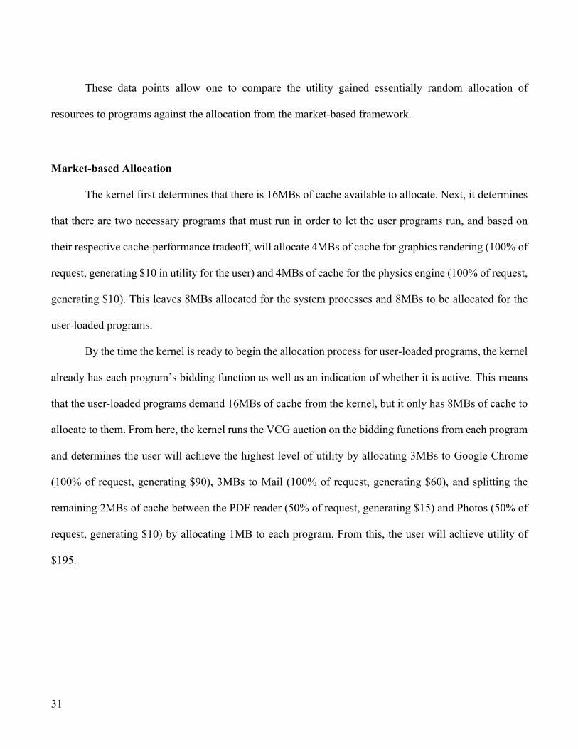
Market-based Allocation

The kernel first determines that there is 16MBs of cache available to allocate. Next, it determines

that there are two necessary programs that must run in order to let the user programs run, and based on

their respective cache-performance tradeoff, will allocate 4MBs of cache for graphics rendering (100% of

request, generating $10 in utility for the user) and 4MBs of cache for the physics engine (100% of request,

generating $10). This leaves 8MBs allocated for the system processes and 8MBs to be allocated for the

user-loaded programs.

By the time the kernel is ready to begin the allocation process for user-loaded programs, the kernel

already has each program’s bidding function as well as an indication of whether it is active. This means

that the user-loaded programs demand 16MBs of cache from the kernel, but it only has 8MBs of cache to

allocate to them. From here, the kernel runs the VCG auction on the bidding functions from each program

and determines the user will achieve the highest level of utility by allocating 3MBs to Google Chrome

(100% of request, generating $90), 3MBs to Mail (100% of request, generating $60), and splitting the

remaining 2MBs of cache between the PDF reader (50% of request, generating $15) and Photos (50% of

request, generating $10) by allocating 1MB to each program. From this, the user will achieve utility of

$195.

32

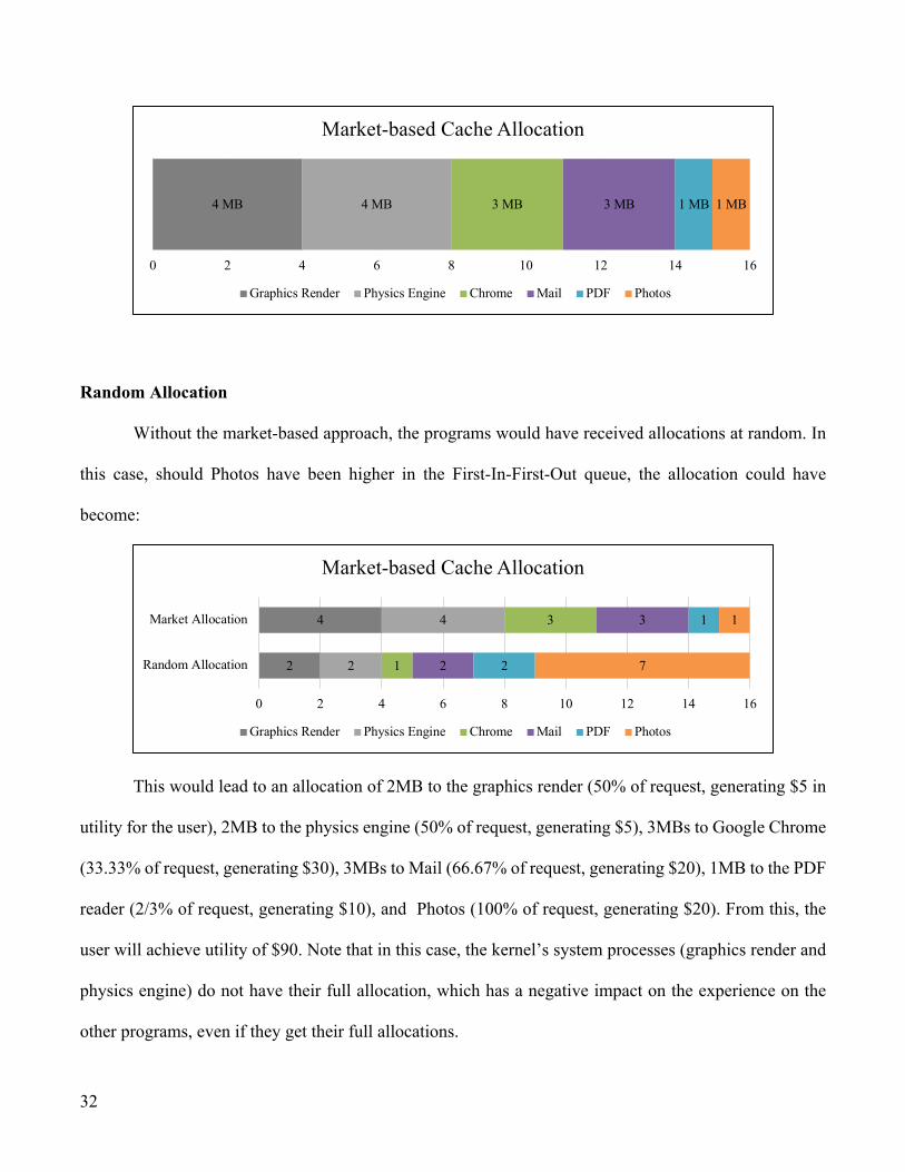
Random Allocation

Without the market-based approach, the programs would have received allocations at random. In

this case, should Photos have been higher in the First-In-First-Out queue, the allocation could have

become:

This would lead to an allocation of 2MB to the graphics render (50% of request, generating $5 in

utility for the user), 2MB to the physics engine (50% of request, generating $5), 3MBs to Google Chrome

(33.33% of request, generating $30), 3MBs to Mail (66.67% of request, generating $20), 1MB to the PDF

reader (2/3% of request, generating $10), and Photos (100% of request, generating $20). From this, the

user will achieve utility of $90. Note that in this case, the kernel’s system processes (graphics render and

physics engine) do not have their full allocation, which has a negative impact on the experience on the

other programs, even if they get their full allocations.

4 MB 4 MB 3 MB 3 MB 1 MB 1 MB

0 2 4 6 8 10 12 14 16

Market-based Cache Allocation

Graphics Render Physics Engine Chrome Mail PDF Photos

2

4

2

4

1

3

2

3

2

1

7

1

0 2 4 6 8 10 12 14 16

Random Allocation

Market Allocation

Market-based Cache Allocation

Graphics Render Physics Engine Chrome Mail PDF Photos

33

Using the market allocation, the highest possible utility is gained every time ($196 in this case),

but a random allocation by definition must have a lower-average payout because it averages every possible

payout case, all but one of which are lower than the optimal payout.

Extension for Multiple Resources

In an effort to narrow the scope of the framework presented in this paper, packages of different

resources were not considered. A further direction of research would be to expand the model presented in

this paper to a package-based auction, where instead of bidding on each resource at a time, each program

has the ability to bid on a collection of resources. In a sense, the problem posed in this paper is one “slice”

of the n-dimensional environment that adding multiple resources would create. Adding the additional

dimensions of multi-resource package allocations would allow the conclusions about optimality to be

extended beyond the tight assumptions made in this paper.

The auction mechanism for these multi-resource bundles can be thought of as a direct extension

of the theoretical framework presented in this paper. One possible extension could be modeled similar to

the auctions used by the Federal Communications Commission (FCC) to auction Spectrum. Connolly and

Kwerel (2007) provide an overview of this process whereby bidders can receive efficient resource-bundle

allocations from the auction even when there are resources with varying levels of substitutability and

complementarity. Within the context of a market-based computing system, the resources could be a

complementary bundle of CPU power and RAM or a substitutable bundle of L2 and L3 processor cache.

An experiment can be conducted–parallel to the one conducted in this paper–on a computer

capable of adjusting multiple resource constraints.31 Once completed, one would have multiple

dimensions of data, which together would form an n-dimensional surface. From this, one can calculate the

31 Beyond the machine used in the experiment outlined in this paper, which was able to adjust the Last Level Cache

34

optimal allocation of resources given the user’s preferences given every allocable resource available

within the computer.

35

Appendix I. Experimental Framework

Although this paper presents a theoretical framework for a computer system, an experiment was

conducted to demonstrate the impact of allocating processor resources on varying workloads. By

combining the hardware and software components discussed within this section, the experiment generated

data from which conclusions were made (described in subsequent chapters).

Hardware Component

The experiment called for a computer containing an Intel processor with a special feature known

as Resource Director Technology.32 In order to understand this technology, it is necessary to have a basic

overview of how a computer processor works and the components that are contained within the chip. Each

chip contains the true “processor” which executes assembly code and a “cache” which is a memory system

containing frequently used data that is divided into tiers to increase the speed of accessing the most used

data.33 The computer’s Resource Director is able to instruct the processor to allocate a certain amount of

cache, in one megabyte34 intervals, to each processor core.

The computer used for this experiment was a Dell PowerEdge R730, which contained one Intel

Xeon E5-2620 v4 processor consisting eight cores and sixteen threads. Each core ran at a base frequency

of 2.10 GHz,35 had 64KB of total L1 Cache, 256 KB of L2 Cache, and 20 MB of L3 Cache, where L3

represented the Last Level Cache (LLC) in the processor. Utilizing the Intel Cache Allocation Technology

(CAT), a series of software tests were able to be run against the same processor with L3 LLC Cache

32 https://www.intel.com/content/www/us/en/architecture-and-technology/resource-director-technology.html 33 https://dl.acm.org/citation.cfm?id=3303977 34 1,000,000 bytes, or 8,000,000 bits. 35 Due to the machine’s configuration, it was not possible to disable Intel Turbo Boost technology.

36

increasing in one-megabyte intervals. The physical hardware of the machine allows for the Intel Resource

Director to allocate in one-megabyte levels from 1MB to 20MBs.

Software Component

Once the physical machine had been configured, a special workload of tasks–known as a

“benchmark”–was run against the various configurations of cache, with the output of each test recorded

for statistical analyses. Benchmarking suites contain set workloads designed to be run across different

environments testing the strengths and weaknesses of the processor configurations. The benchmark

control program acts as a stationmaster for the individual workload programs, measuring how quickly

they complete in units of time, and utilizing this data to calculate an overall value for the running of all of

the elements of the workload.

Geekbench v5.0.2 was the benchmark suite selected for this experiment. Geekbench was chosen

for three primary reasons: 1) it tests a workload of modern algorithms36 including Machine Learning (ML)

and Augmented Reality (AR) as well as every-day tasks of encryption and text-based rendering that are

well defined within both academia and industry;37 2) it has macro and micro elements, meaning that it

outputs information from each algorithm run as well as composite scores for an entire workload computed;

3) it runs the algorithms in single-core and multi-core configurations. When selecting a multi-core

benchmark, it is important to look for one which distributes one algorithm’s tasks across various cores. If

the same algorithm is run on each core, then the performance will scale linearly; however, if the algorithm

is divided as is the case with Geekbench 5, then the performance will experience diminishing marginal

36 Modern as defined by usage in 2019. 37 There are nearly half-a-million runs of this benchmarking suite across various processors, from server, desktop,

laptop, and mobile devices.

37

returns to both processor cores and the memory that is used to connect them and store data–especially the

Last Level Cache (LLC), which is used in the physical part of this experiment.

Almost any modern processor in the world can be compared with this suite, which runs a workload

including “data compression, image processing, machine learning, and physics simulation” designed “to

evaluate and optimize CPU and memory performance.” The workloads are split into Cryptography

Workloads, Integer Workloads, and Floating Point workloads, as each is able to test the abilities of

different sub-circuits within the processor, each designed to utilize cache memory differently.38 The

software itself provides the output of the relative time39 required to run each test in seconds, and these

scores can be combined through a weighted average to simulate almost any workload–be it that of an end

user on a Laptop or that of a server in a Data Center.

The experiment consisted of running the Geekbench 5 workload at each cache allocation (1MB,

2MB…20MB), and the experiment was run five-times in total so that outliers could be analyzed. The

results of the tests and corresponding analysis available in the Data section of this paper.

Cryptography Workloads

For the Cryptography Workloads, the suite runs a single algorithm known as Advanced Encryption

Standard (“AES”).40 The algorithm makes use of special circuitry available in the Intel processors

allowing for a feature called hardware encryption, which reduces the amount of computation necessary

for the computer to perform the encryption. This test interacts with the memory as the encryption sub-

circuitry will utilize the cache to store the data from the 256-bit key and the large multiplication. Although

this type of encryption is not directly user facing, most computers today operate with an encrypted hard

38 Geekbench specifications from https://www.geekbench.com/doc/geekbench5-cpu-workloads.pdf 39 The relative time is calculated by taking the time known to the CPU immediately before the test was run subtracted

from the time known just before the test was run. 40 See Geekbench specifications.

38

drive, meant to keep data secure in the event that the machine is physical attacked. The data on the drive

is decrypted when needed by the user to access files, causing the algorithm to run in the background on

consumer phones and computers.

Integer Workloads

In Computer Science, “integers” are numbers without decimal places can represent 2W unique

numbers, where 𝑥 represents the number of bits that the computer can physical remember and perform

computations.41 For the Integer Workloads, the suite runs the following algorithms:42 Markov Text

Compression, JPEG and PNG Image Compressions, Shortest Paths in Graphs with Dijkstra’s algorithm,

HTML5 Website Rendering, In-memory SQLite Database execution, PDF rendering, Markdown-

formatted Text Rendering, C code compilation for the AArch64 platform.

Floating Point Workloads

In Computer Science, “floating point” numbers represent decimal numbers (i.e. ℝ the real

numbers). These numbers are not represented the same way that integers are and due to the fixed number

of bits on the system, 𝑥, create a range vs. accuracy dilemma.43 For the Floating Point Workloads, the

suite runs algorithms computing N-Body Physics, Rigid Body Physics, Gaussian Blur, Face Detection,

Horizon Detection, Image Reconstruction / “Content Aware Fill,” High Dynamic Range image

processing, Ray Tracing, Augmented Reality motion structure construction, Speech Recognition, and

Convolutional Neural Network image classification / Machine Learning.44

41 As of this writing, common computer architectures allow for 32-bit and 64-bit processing. 42 See Geekbench specifications. 43 Within the same 𝑥 bits, you can store either a large number or a small number with many decimal places as the bits

merely store a certain amount of permutations of 1s and 0s. 44 See Geekbench specifications.

39

More details of each algorithm are provided in the Data section of this paper and in the cited

whitepaper produced by the developer of Geekbench.

40

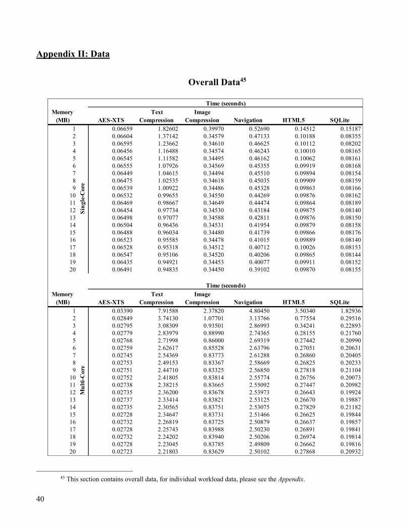
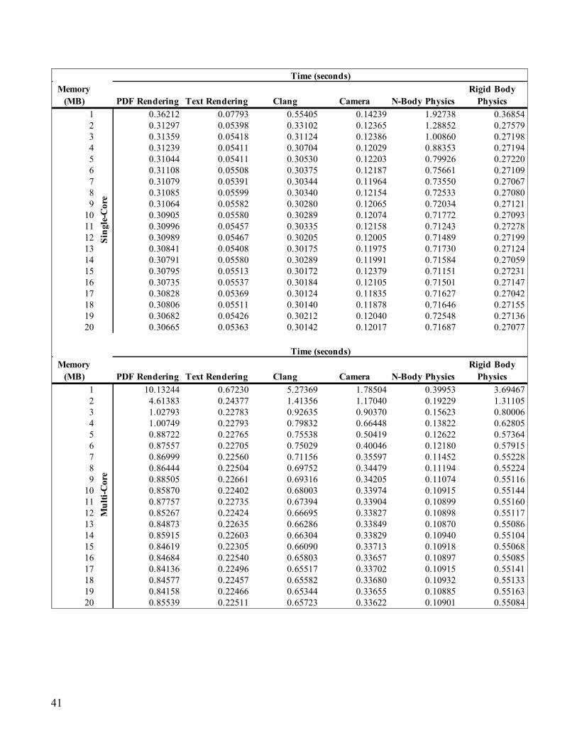
Appendix II: Data

Overall Data45

45 This section contains overall data, for individual workload data, please see the Appendix.

Memory (MB) AES-XTS

Text Compression

Image Compression Navigation HTML5 SQLite

1 0.06659 1.82602 0.39970 0.52690 0.14512 0.151872 0.06604 1.37142 0.34579 0.47133 0.10188 0.083553 0.06595 1.23662 0.34610 0.46625 0.10112 0.082024 0.06456 1.16488 0.34574 0.46243 0.10010 0.081655 0.06545 1.11582 0.34495 0.46162 0.10062 0.081616 0.06555 1.07926 0.34569 0.45355 0.09919 0.081687 0.06449 1.04615 0.34494 0.45510 0.09894 0.081548 0.06475 1.02535 0.34618 0.45035 0.09909 0.081599 0.06539 1.00922 0.34486 0.45328 0.09863 0.0816610 0.06532 0.99655 0.34550 0.44269 0.09876 0.0816211 0.06469 0.98667 0.34649 0.44474 0.09864 0.0818912 0.06454 0.97734 0.34530 0.43184 0.09875 0.0814013 0.06498 0.97077 0.34588 0.42811 0.09876 0.0815014 0.06504 0.96436 0.34531 0.41954 0.09879 0.0815815 0.06488 0.96034 0.34480 0.41739 0.09866 0.0817616 0.06523 0.95585 0.34478 0.41015 0.09889 0.0814017 0.06528 0.95318 0.34512 0.40712 0.10026 0.0815318 0.06547 0.95106 0.34520 0.40206 0.09865 0.0814419 0.06435 0.94921 0.34453 0.40077 0.09911 0.0815220 0.06491 0.94835 0.34450 0.39102 0.09870 0.08155

Memory (MB) AES-XTS

Text Compression

Image Compression Navigation HTML5 SQLite

1 0.03390 7.91588 2.37820 4.80450 3.50340 1.829362 0.02849 3.74130 1.07701 3.13766 0.77554 0.295163 0.02795 3.08309 0.93501 2.86993 0.34241 0.228934 0.02779 2.83979 0.88990 2.74365 0.28155 0.217605 0.02768 2.71998 0.86000 2.69319 0.27442 0.209906 0.02759 2.62617 0.85528 2.63796 0.27051 0.206317 0.02745 2.54369 0.83773 2.61288 0.26860 0.204058 0.02753 2.49153 0.83367 2.58669 0.26825 0.202339 0.02751 2.44710 0.83325 2.56850 0.27818 0.2110410 0.02752 2.41805 0.83814 2.55774 0.26756 0.2007311 0.02738 2.38215 0.83665 2.55092 0.27447 0.2098212 0.02735 2.36200 0.83678 2.53973 0.26643 0.1992413 0.02737 2.33414 0.83821 2.53125 0.26670 0.1988714 0.02735 2.30565 0.83751 2.53075 0.27829 0.2118215 0.02728 2.34647 0.83731 2.51466 0.26625 0.1984416 0.02732 2.26819 0.83725 2.50879 0.26637 0.1985717 0.02728 2.25743 0.83988 2.50230 0.26891 0.1984118 0.02732 2.24202 0.83940 2.50206 0.26974 0.1981419 0.02728 2.23045 0.83785 2.49809 0.26662 0.1981620 0.02723 2.21803 0.83629 2.50102 0.27868 0.20932

Time (seconds)

Sing

le-C

ore

Mul

ti-C

ore

Time (seconds)

41

Memory (MB) PDF Rendering Text Rendering Clang Camera N-Body Physics

Rigid Body Physics

1 0.36212 0.07793 0.55405 0.14239 1.92738 0.368542 0.31297 0.05398 0.33102 0.12365 1.28852 0.275793 0.31359 0.05418 0.31124 0.12386 1.00860 0.271984 0.31239 0.05411 0.30704 0.12029 0.88353 0.271945 0.31044 0.05411 0.30530 0.12203 0.79926 0.272206 0.31108 0.05508 0.30375 0.12187 0.75661 0.271097 0.31079 0.05391 0.30344 0.11964 0.73550 0.270678 0.31085 0.05599 0.30340 0.12154 0.72533 0.270809 0.31064 0.05582 0.30280 0.12065 0.72034 0.2712110 0.30905 0.05580 0.30289 0.12074 0.71772 0.2709311 0.30996 0.05457 0.30335 0.12158 0.71243 0.2727812 0.30989 0.05467 0.30205 0.12005 0.71489 0.2719913 0.30841 0.05408 0.30175 0.11975 0.71730 0.2712414 0.30791 0.05580 0.30289 0.11991 0.71584 0.2705915 0.30795 0.05513 0.30172 0.12379 0.71151 0.2723116 0.30735 0.05537 0.30184 0.12105 0.71501 0.2714717 0.30828 0.05369 0.30124 0.11835 0.71627 0.2704218 0.30806 0.05511 0.30140 0.11878 0.71646 0.2715519 0.30682 0.05426 0.30212 0.12040 0.72548 0.2713620 0.30665 0.05363 0.30142 0.12017 0.71687 0.27077

Memory (MB) PDF Rendering Text Rendering Clang Camera N-Body Physics

Rigid Body Physics

1 10.13244 0.67230 5.27369 1.78504 0.39953 3.694672 4.61383 0.24377 1.41356 1.17040 0.19229 1.311053 1.02793 0.22783 0.92635 0.90370 0.15623 0.800064 1.00749 0.22793 0.79832 0.66448 0.13822 0.628055 0.88722 0.22765 0.75538 0.50419 0.12622 0.573646 0.87557 0.22705 0.75029 0.40046 0.12180 0.579157 0.86999 0.22560 0.71156 0.35597 0.11452 0.552288 0.86444 0.22504 0.69752 0.34479 0.11194 0.552249 0.88505 0.22661 0.69316 0.34205 0.11074 0.5511610 0.85870 0.22402 0.68003 0.33974 0.10915 0.5514411 0.87757 0.22735 0.67394 0.33904 0.10899 0.5516012 0.85267 0.22424 0.66695 0.33827 0.10898 0.5511713 0.84873 0.22635 0.66286 0.33849 0.10870 0.5508614 0.85915 0.22603 0.66304 0.33829 0.10940 0.5510415 0.84619 0.22305 0.66090 0.33713 0.10918 0.5506816 0.84684 0.22540 0.65803 0.33657 0.10897 0.5508517 0.84136 0.22496 0.65517 0.33702 0.10915 0.5514118 0.84577 0.22457 0.65582 0.33680 0.10932 0.5513319 0.84158 0.22466 0.65344 0.33655 0.10885 0.5516320 0.85539 0.22511 0.65723 0.33622 0.10901 0.55084

Time (seconds)

Sing

le-C

ore

Mul

ti-C

ore

Time (seconds)

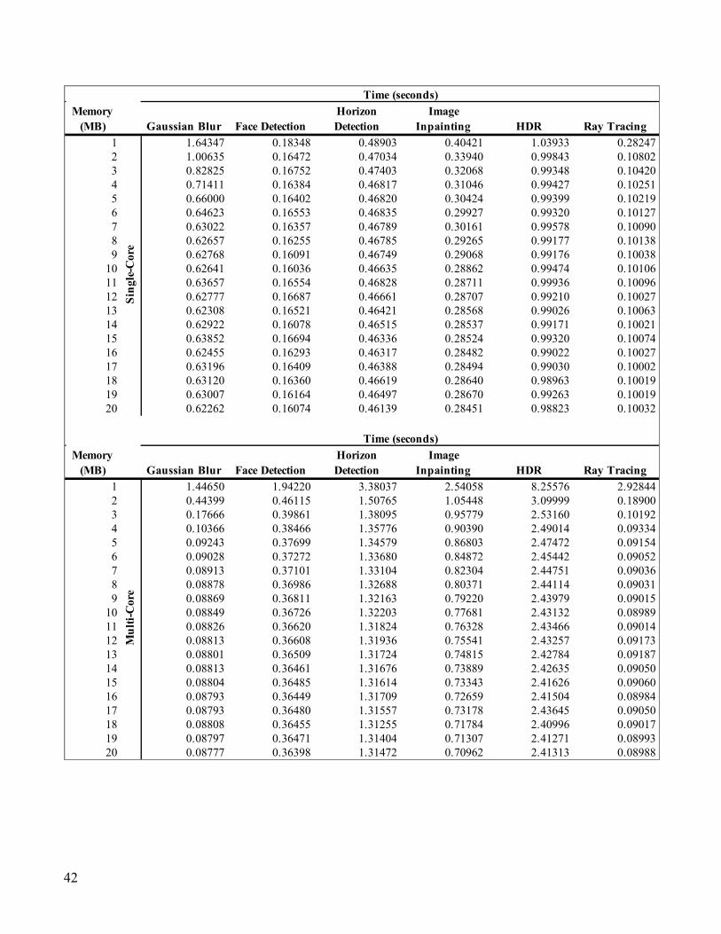
42

Memory (MB) Gaussian Blur Face Detection

Horizon Detection

Image Inpainting HDR Ray Tracing

1 1.64347 0.18348 0.48903 0.40421 1.03933 0.282472 1.00635 0.16472 0.47034 0.33940 0.99843 0.108023 0.82825 0.16752 0.47403 0.32068 0.99348 0.104204 0.71411 0.16384 0.46817 0.31046 0.99427 0.102515 0.66000 0.16402 0.46820 0.30424 0.99399 0.102196 0.64623 0.16553 0.46835 0.29927 0.99320 0.101277 0.63022 0.16357 0.46789 0.30161 0.99578 0.100908 0.62657 0.16255 0.46785 0.29265 0.99177 0.101389 0.62768 0.16091 0.46749 0.29068 0.99176 0.1003810 0.62641 0.16036 0.46635 0.28862 0.99474 0.1010611 0.63657 0.16554 0.46828 0.28711 0.99936 0.1009612 0.62777 0.16687 0.46661 0.28707 0.99210 0.1002713 0.62308 0.16521 0.46421 0.28568 0.99026 0.1006314 0.62922 0.16078 0.46515 0.28537 0.99171 0.1002115 0.63852 0.16694 0.46336 0.28524 0.99320 0.1007416 0.62455 0.16293 0.46317 0.28482 0.99022 0.1002717 0.63196 0.16409 0.46388 0.28494 0.99030 0.1000218 0.63120 0.16360 0.46619 0.28640 0.98963 0.1001919 0.63007 0.16164 0.46497 0.28670 0.99263 0.1001920 0.62262 0.16074 0.46139 0.28451 0.98823 0.10032

Memory (MB) Gaussian Blur Face Detection

Horizon Detection

Image Inpainting HDR Ray Tracing

1 1.44650 1.94220 3.38037 2.54058 8.25576 2.928442 0.44399 0.46115 1.50765 1.05448 3.09999 0.189003 0.17666 0.39861 1.38095 0.95779 2.53160 0.101924 0.10366 0.38466 1.35776 0.90390 2.49014 0.093345 0.09243 0.37699 1.34579 0.86803 2.47472 0.091546 0.09028 0.37272 1.33680 0.84872 2.45442 0.090527 0.08913 0.37101 1.33104 0.82304 2.44751 0.090368 0.08878 0.36986 1.32688 0.80371 2.44114 0.090319 0.08869 0.36811 1.32163 0.79220 2.43979 0.0901510 0.08849 0.36726 1.32203 0.77681 2.43132 0.0898911 0.08826 0.36620 1.31824 0.76328 2.43466 0.0901412 0.08813 0.36608 1.31936 0.75541 2.43257 0.0917313 0.08801 0.36509 1.31724 0.74815 2.42784 0.0918714 0.08813 0.36461 1.31676 0.73889 2.42635 0.0905015 0.08804 0.36485 1.31614 0.73343 2.41626 0.0906016 0.08793 0.36449 1.31709 0.72659 2.41504 0.0898417 0.08793 0.36480 1.31557 0.73178 2.43645 0.0905018 0.08808 0.36455 1.31255 0.71784 2.40996 0.0901719 0.08797 0.36471 1.31404 0.71307 2.41271 0.0899320 0.08777 0.36398 1.31472 0.70962 2.41313 0.08988

Time (seconds)

Sing

le-C

ore

Mul

ti-C

ore

Time (seconds)

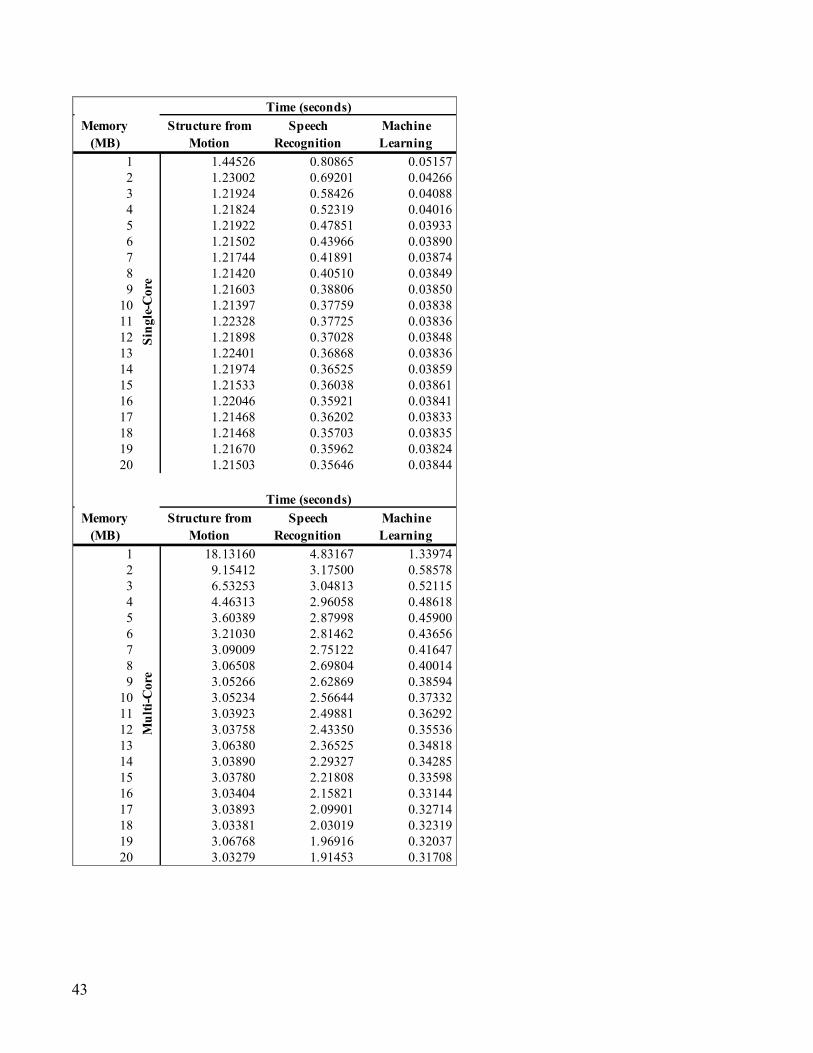
43

Memory (MB)

Structure from Motion

Speech Recognition

Machine Learning

1 1.44526 0.80865 0.051572 1.23002 0.69201 0.042663 1.21924 0.58426 0.040884 1.21824 0.52319 0.040165 1.21922 0.47851 0.039336 1.21502 0.43966 0.038907 1.21744 0.41891 0.038748 1.21420 0.40510 0.038499 1.21603 0.38806 0.0385010 1.21397 0.37759 0.0383811 1.22328 0.37725 0.0383612 1.21898 0.37028 0.0384813 1.22401 0.36868 0.0383614 1.21974 0.36525 0.0385915 1.21533 0.36038 0.0386116 1.22046 0.35921 0.0384117 1.21468 0.36202 0.0383318 1.21468 0.35703 0.0383519 1.21670 0.35962 0.0382420 1.21503 0.35646 0.03844

Memory (MB)

Structure from Motion

Speech Recognition

Machine Learning

1 18.13160 4.83167 1.339742 9.15412 3.17500 0.585783 6.53253 3.04813 0.521154 4.46313 2.96058 0.486185 3.60389 2.87998 0.459006 3.21030 2.81462 0.436567 3.09009 2.75122 0.416478 3.06508 2.69804 0.400149 3.05266 2.62869 0.3859410 3.05234 2.56644 0.3733211 3.03923 2.49881 0.3629212 3.03758 2.43350 0.3553613 3.06380 2.36525 0.3481814 3.03890 2.29327 0.3428515 3.03780 2.21808 0.3359816 3.03404 2.15821 0.3314417 3.03893 2.09901 0.3271418 3.03381 2.03019 0.3231919 3.06768 1.96916 0.3203720 3.03279 1.91453 0.31708

Time (seconds)

Time (seconds)

Sing

le-C

ore

Mul

ti-C

ore

44

Appendix IV: Individual Workloads

Cryptography Workload: AES-XTS

Statistical Analysis

Graphical Representations

Memory (MB) σ

Coefficient of Variation σ

Coefficient of Variation

1 0.00049 0.00730 0.00344 0.101522 0.00163 0.02475 0.00068 0.023943 0.00150 0.02270 0.00015 0.005364 0.00019 0.00297 0.00014 0.005135 0.00129 0.01969 0.00022 0.008046 0.00171 0.02608 0.00021 0.007537 0.00031 0.00487 0.00006 0.002138 0.00080 0.01241 0.00020 0.007449 0.00147 0.02252 0.00039 0.0140610 0.00144 0.02212 0.00018 0.0064011 0.00086 0.01334 0.00025 0.0089512 0.00036 0.00564 0.00012 0.0043913 0.00118 0.01822 0.00010 0.0035914 0.00116 0.01783 0.00021 0.0078415 0.00098 0.01514 0.00008 0.0028916 0.00130 0.01998 0.00020 0.0074017 0.00113 0.01736 0.00016 0.0057018 0.00136 0.02071 0.00019 0.0069619 0.00017 0.00262 0.00017 0.0062420 0.00115 0.01765 0.00008 0.00302

Single-Core Multi-Core

0.06

0.06

0.06

0.06

0.07

0.07

0.07

0.07

0.07

1 2 3 4 5 6 7 8 9 10 11 12 13 14 15 16 17 18 19 20

Tim

e (s

)

Last Level Cache Allocation (MBs)

Single Core

0.00

0.01

0.01

0.02

0.02

0.03

0.03

0.04

0.04

1 2 3 4 5 6 7 8 9 10 11 12 13 14 15 16 17 18 19 20

Tim

e (s

)

Last Level Cache Allocation (MBs)

Multi Core

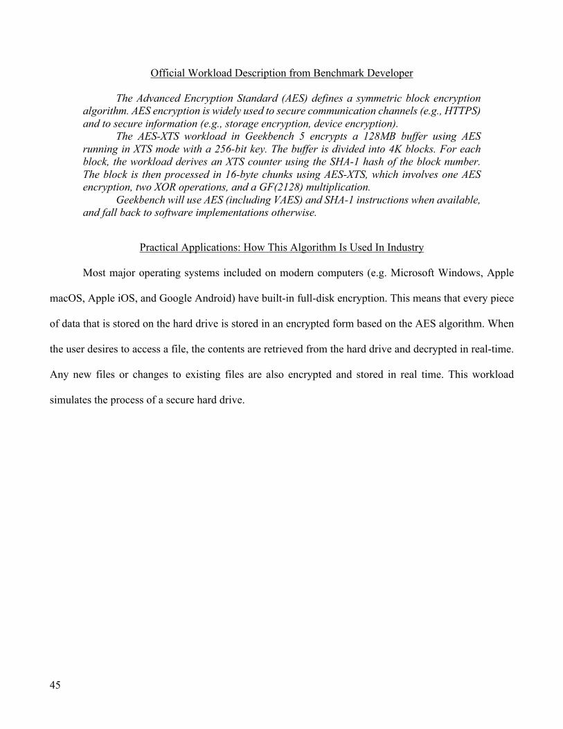
45

Official Workload Description from Benchmark Developer

The Advanced Encryption Standard (AES) defines a symmetric block encryption algorithm. AES encryption is widely used to secure communication channels (e.g., HTTPS) and to secure information (e.g., storage encryption, device encryption).

The AES-XTS workload in Geekbench 5 encrypts a 128MB buffer using AES running in XTS mode with a 256-bit key. The buffer is divided into 4K blocks. For each block, the workload derives an XTS counter using the SHA-1 hash of the block number. The block is then processed in 16-byte chunks using AES-XTS, which involves one AES encryption, two XOR operations, and a GF(2128) multiplication.

Geekbench will use AES (including VAES) and SHA-1 instructions when available, and fall back to software implementations otherwise.

Practical Applications: How This Algorithm Is Used In Industry

Most major operating systems included on modern computers (e.g. Microsoft Windows, Apple

macOS, Apple iOS, and Google Android) have built-in full-disk encryption. This means that every piece

of data that is stored on the hard drive is stored in an encrypted form based on the AES algorithm. When

the user desires to access a file, the contents are retrieved from the hard drive and decrypted in real-time.

Any new files or changes to existing files are also encrypted and stored in real time. This workload

simulates the process of a secure hard drive.

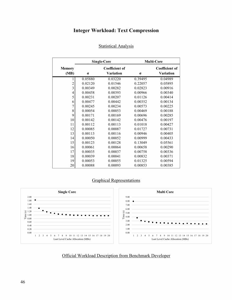
46

Integer Workload: Text Compression

Statistical Analysis

Graphical Representations

Official Workload Description from Benchmark Developer

Memory (MB) σ

Coefficient of Variation σ

Coefficient of Variation

1 0.05880 0.03220 0.39495 0.049892 0.02120 0.01546 0.22057 0.058953 0.00349 0.00282 0.02823 0.009164 0.00458 0.00393 0.00966 0.003405 0.00231 0.00207 0.01126 0.004146 0.00477 0.00442 0.00352 0.001347 0.00245 0.00234 0.00573 0.002258 0.00054 0.00053 0.00469 0.001889 0.00171 0.00169 0.00696 0.0028510 0.00142 0.00142 0.00476 0.0019711 0.00112 0.00113 0.01018 0.0042712 0.00085 0.00087 0.01727 0.0073113 0.00113 0.00116 0.00946 0.0040514 0.00050 0.00052 0.00999 0.0043315 0.00123 0.00128 0.13049 0.0556116 0.00061 0.00064 0.00658 0.0029017 0.00035 0.00037 0.00758 0.0033618 0.00039 0.00041 0.00832 0.0037119 0.00053 0.00055 0.01325 0.0059420 0.00088 0.00093 0.00853 0.00385

Single-Core Multi-Core

0.000.200.400.600.801.001.201.401.601.802.00

1 2 3 4 5 6 7 8 9 10 11 12 13 14 15 16 17 18 19 20

Tim

e (s

)

Last Level Cache Allocation (MBs)

Single Core

0.001.00

2.003.00

4.005.006.00

7.008.00

9.00

1 2 3 4 5 6 7 8 9 10 11 12 13 14 15 16 17 18 19 20

Tim

e (s

)

Last Level Cache Allocation (MBs)

Multi Core

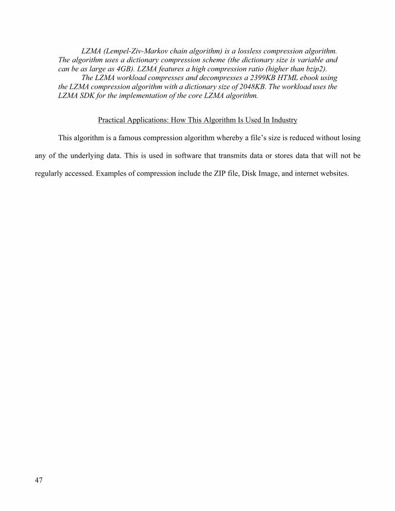
47

LZMA (Lempel-Ziv-Markov chain algorithm) is a lossless compression algorithm. The algorithm uses a dictionary compression scheme (the dictionary size is variable and can be as large as 4GB). LZMA features a high compression ratio (higher than bzip2).

The LZMA workload compresses and decompresses a 2399KB HTML ebook using the LZMA compression algorithm with a dictionary size of 2048KB. The workload uses the LZMA SDK for the implementation of the core LZMA algorithm.

Practical Applications: How This Algorithm Is Used In Industry

This algorithm is a famous compression algorithm whereby a file’s size is reduced without losing

any of the underlying data. This is used in software that transmits data or stores data that will not be

regularly accessed. Examples of compression include the ZIP file, Disk Image, and internet websites.

48

Integer Workload: Image Compression

Statistical Analysis

Graphical Representations

Official Workload Description from Benchmark Developer

Memory (MB) σ

Coefficient of Variation σ

Coefficient of Variation

1 0.03044 0.07615 0.29502 0.124052 0.00119 0.00344 0.00919 0.008543 0.00108 0.00312 0.00778 0.008324 0.00104 0.00300 0.00777 0.008735 0.00013 0.00037 0.00833 0.009696 0.00154 0.00446 0.00554 0.006477 0.00036 0.00106 0.00409 0.004888 0.00108 0.00313 0.00620 0.007449 0.00018 0.00053 0.00444 0.0053310 0.00061 0.00176 0.00267 0.0031911 0.00136 0.00393 0.00179 0.0021412 0.00127 0.00367 0.00387 0.0046313 0.00102 0.00294 0.00427 0.0050914 0.00103 0.00298 0.00294 0.0035215 0.00114 0.00330 0.00166 0.0019916 0.00069 0.00200 0.00193 0.0023117 0.00114 0.00331 0.00271 0.0032218 0.00139 0.00403 0.00129 0.0015419 0.00026 0.00076 0.00133 0.0015920 0.00055 0.00158 0.00375 0.00449

Single-Core Multi-Core

0.310.320.330.340.350.360.370.380.390.400.41

1 2 3 4 5 6 7 8 9 10 11 12 13 14 15 16 17 18 19 20

Tim

e (s

)

Last Level Cache Allocation (MBs)

Single Core

0.00

0.50

1.00

1.50

2.00

2.50

1 2 3 4 5 6 7 8 9 10 11 12 13 14 15 16 17 18 19 20

Tim

e (s

)

Last Level Cache Allocation (MBs)

Multi Core

49

The Image Compression workload compresses and decompresses a photograph using JPEG, and a CSS sprite using PNG. The workload sets the JPEG quality parameter to “90”, a commonly-used setting for users who desire high-quality images.

The workload uses libjpeg-turbo for the implementation of the core JPEG algorithm, and libpng for the implementation of the core PNG algorithm.

Practical Applications: How This Algorithm Is Used In Industry

This algorithm is commonly used in videoconferencing and social media applications. For video

and audio communications, the data being recorded by the computer’s camera needs to be converted from

the post-processed “raw” file that typically takes up several megabytes to a size small enough to send 30

images per second across the internet with little latency. The longer this process takes, the larger latency

or lag exists between you and the person on the other end of the video call and the choppier the video will

be as there will be fewer frames sent per second. For social media applications (e.g. Instagram, Snapchat)

and multimedia libraries (e.g. Apple’s Photos, Google Photos), this algorithm is used to export photos

from a library and send them across the internet.

50

Integer Workload: Navigation

Statistical Analysis

Graphical Representations

Official Workload Description from Benchmark Developer

The Navigation workload computes driving directions between a sequence of destinations using Dijkstra's algorithm. Similar techniques are used to compute paths in

Memory (MB) σ

Coefficient of Variation σ

Coefficient of Variation

1 0.00541 0.01026 0.33442 0.069602 0.00459 0.00973 0.06581 0.020973 0.00978 0.02097 0.03905 0.013614 0.01070 0.02313 0.01037 0.003785 0.01093 0.02368 0.01666 0.006196 0.00155 0.00341 0.00593 0.002257 0.00880 0.01934 0.00425 0.001638 0.00202 0.00448 0.00489 0.001899 0.01133 0.02499 0.00424 0.0016510 0.00349 0.00789 0.00328 0.0012811 0.01097 0.02466 0.00659 0.0025812 0.00131 0.00303 0.00399 0.0015713 0.00371 0.00866 0.00336 0.0013314 0.00064 0.00151 0.01062 0.0041915 0.00306 0.00734 0.00477 0.0019016 0.00107 0.00260 0.00235 0.0009417 0.00451 0.01109 0.00543 0.0021718 0.00213 0.00530 0.00451 0.0018019 0.00852 0.02127 0.00519 0.0020820 0.00189 0.00484 0.01063 0.00425

Single-Core Multi-Core

0.00

0.10

0.20

0.30

0.40

0.50

0.60

1 2 3 4 5 6 7 8 9 10 11 12 13 14 15 16 17 18 19 20

Tim

e (s

)

Last Level Cache Allocation (MBs)

Single Core

0.00

1.00

2.00

3.00

4.00

5.00

6.00

1 2 3 4 5 6 7 8 9 10 11 12 13 14 15 16 17 18 19 20

Tim

e (s

)

Last Level Cache Allocation (MBs)

Multi Core

51

games, to route computer network traffic, and to route driving directions. The dataset contains 216,548 nodes and 450,277 edges with weights approximating travel time along the road represented by the edge. The route includes 13 destinations. The dataset is based on Open Street Map data for Ontario, Canada.

Practical Applications: How This Algorithm Is Used In Industry

Although this set of tasks is mostly known to calculate directions in map applications, it is general

in the sense that the underlying Dijkstra’s algorithm can be used to compute the shortest path of graphs

where all edges of the graph have positive weights. This is commonly used in modeling any problem that

can be represented as a graph, which relates to finding the number of connections between people in a

photo library or friend network. Given multiple datasets that have overlapping properties, this algorithm

will find the most efficient way to get from one point to any other given point, if at least one connection

exists.

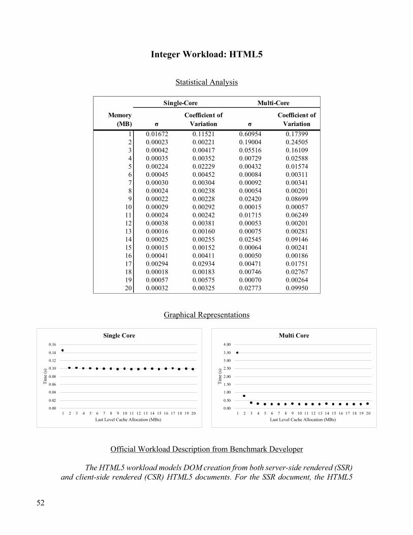
52

Integer Workload: HTML5

Statistical Analysis

Graphical Representations

Official Workload Description from Benchmark Developer

The HTML5 workload models DOM creation from both server-side rendered (SSR) and client-side rendered (CSR) HTML5 documents. For the SSR document, the HTML5

Memory (MB) σ

Coefficient of Variation σ

Coefficient of Variation

1 0.01672 0.11521 0.60954 0.173992 0.00023 0.00221 0.19004 0.245053 0.00042 0.00417 0.05516 0.161094 0.00035 0.00352 0.00729 0.025885 0.00224 0.02229 0.00432 0.015746 0.00045 0.00452 0.00084 0.003117 0.00030 0.00304 0.00092 0.003418 0.00024 0.00238 0.00054 0.002019 0.00022 0.00228 0.02420 0.0869910 0.00029 0.00292 0.00015 0.0005711 0.00024 0.00242 0.01715 0.0624912 0.00038 0.00381 0.00053 0.0020113 0.00016 0.00160 0.00075 0.0028114 0.00025 0.00255 0.02545 0.0914615 0.00015 0.00152 0.00064 0.0024116 0.00041 0.00411 0.00050 0.0018617 0.00294 0.02934 0.00471 0.0175118 0.00018 0.00183 0.00746 0.0276719 0.00057 0.00575 0.00070 0.0026420 0.00032 0.00325 0.02773 0.09950

Single-Core Multi-Core

0.00

0.02

0.04

0.06

0.08

0.10

0.12

0.14

0.16

1 2 3 4 5 6 7 8 9 10 11 12 13 14 15 16 17 18 19 20

Tim

e (s

)

Last Level Cache Allocation (MBs)

Single Core

0.00

0.50

1.00

1.50

2.00

2.50

3.00

3.50

4.00

1 2 3 4 5 6 7 8 9 10 11 12 13 14 15 16 17 18 19 20

Tim

e (s

)

Last Level Cache Allocation (MBs)

Multi Core

53

workload uses the Gumbo HTML5 parser to create the DOM by parsing an HTML file. For the CSR document, the HTML5 workload uses the Gumbo HTML5 parser to create the DOM by parsing an HTML file, then uses the Duktape JavaScript engine to extend the DOM.

Practical Applications: How This Algorithm Is Used In Industry

This workload renders a webpage as if the user navigated to it in a web browser (e.g. Google

Chrome, Safari, or Firefox). This is likely a very common workload for any user of a personal computer.

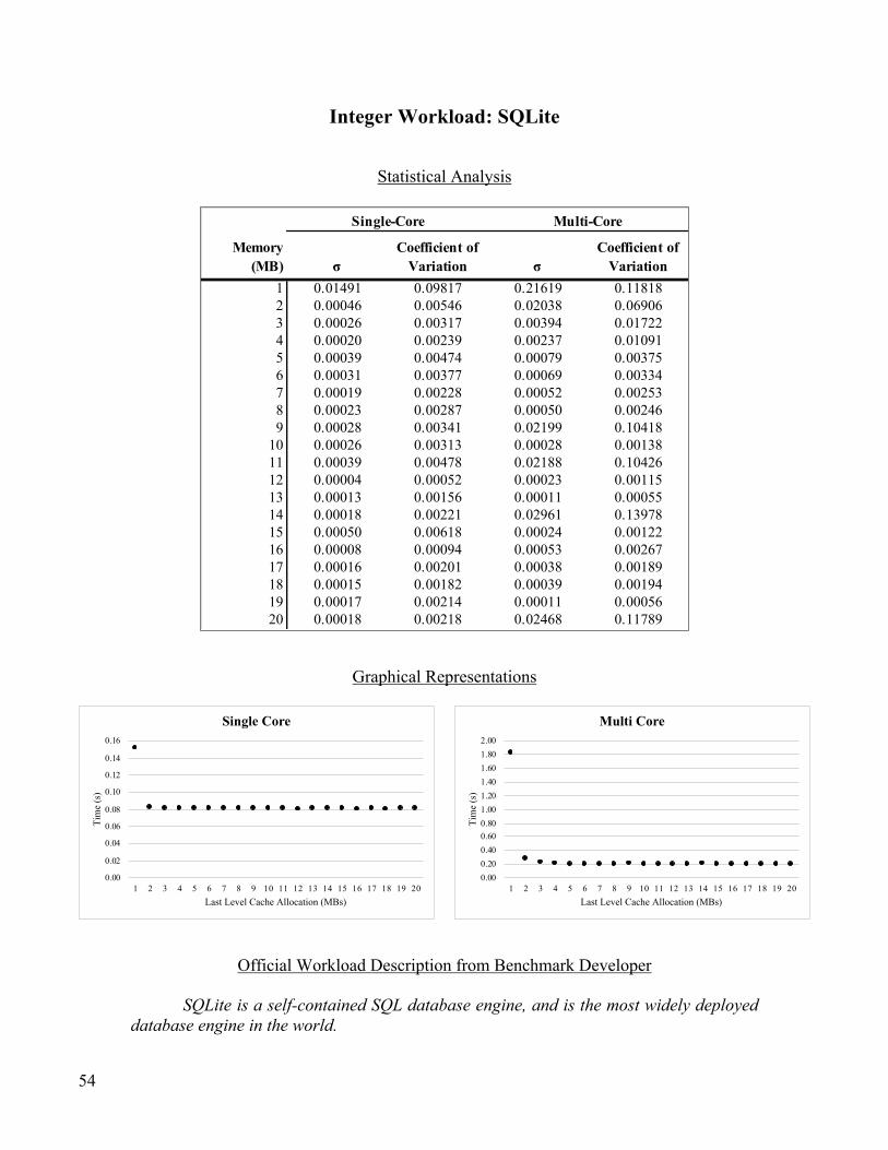
54

Integer Workload: SQLite

Statistical Analysis

Graphical Representations

Official Workload Description from Benchmark Developer

SQLite is a self-contained SQL database engine, and is the most widely deployed database engine in the world.

Memory (MB) σ

Coefficient of Variation σ

Coefficient of Variation

1 0.01491 0.09817 0.21619 0.118182 0.00046 0.00546 0.02038 0.069063 0.00026 0.00317 0.00394 0.017224 0.00020 0.00239 0.00237 0.010915 0.00039 0.00474 0.00079 0.003756 0.00031 0.00377 0.00069 0.003347 0.00019 0.00228 0.00052 0.002538 0.00023 0.00287 0.00050 0.002469 0.00028 0.00341 0.02199 0.1041810 0.00026 0.00313 0.00028 0.0013811 0.00039 0.00478 0.02188 0.1042612 0.00004 0.00052 0.00023 0.0011513 0.00013 0.00156 0.00011 0.0005514 0.00018 0.00221 0.02961 0.1397815 0.00050 0.00618 0.00024 0.0012216 0.00008 0.00094 0.00053 0.0026717 0.00016 0.00201 0.00038 0.0018918 0.00015 0.00182 0.00039 0.0019419 0.00017 0.00214 0.00011 0.0005620 0.00018 0.00218 0.02468 0.11789

Single-Core Multi-Core

0.00

0.02

0.04

0.06

0.08

0.10

0.12

0.14

0.16

1 2 3 4 5 6 7 8 9 10 11 12 13 14 15 16 17 18 19 20

Tim

e (s

)

Last Level Cache Allocation (MBs)

Single Core

0.000.200.400.600.801.001.201.401.601.802.00

1 2 3 4 5 6 7 8 9 10 11 12 13 14 15 16 17 18 19 20

Tim

e (s

)

Last Level Cache Allocation (MBs)

Multi Core

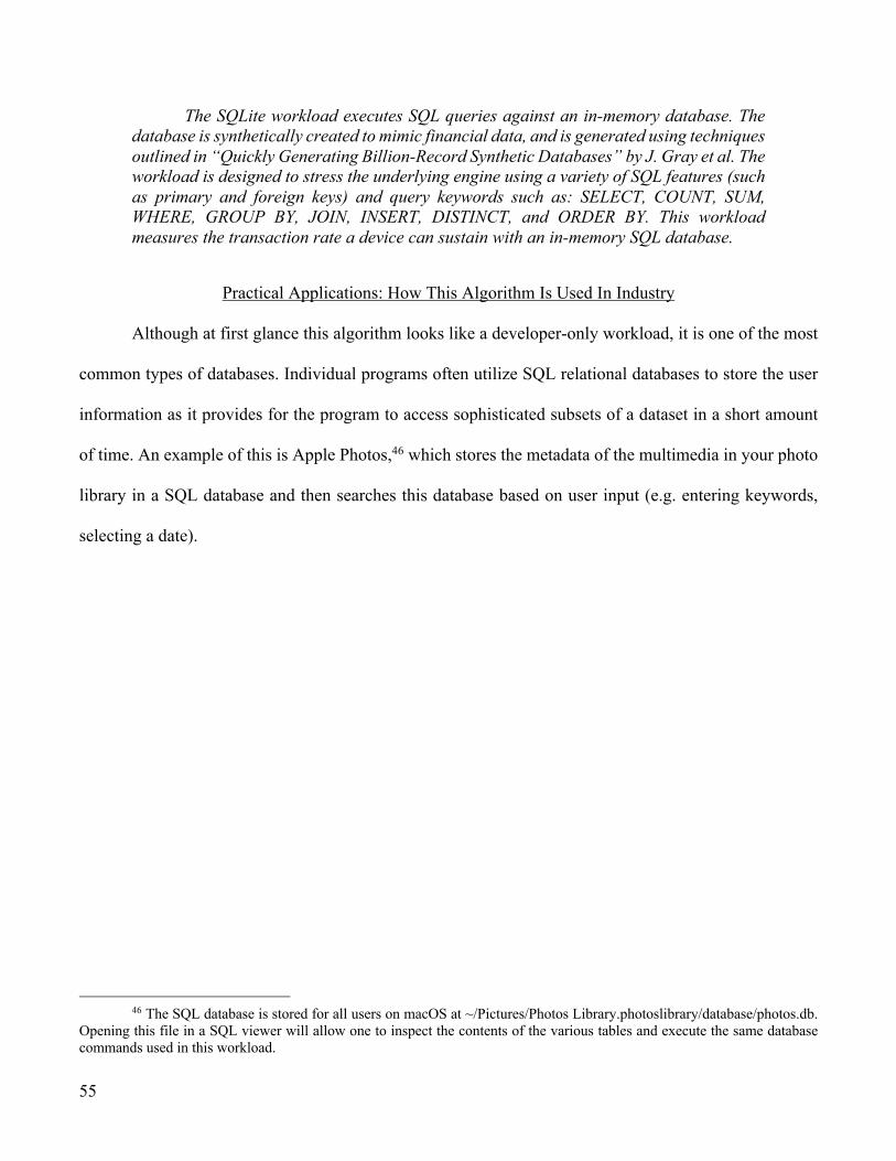
55

The SQLite workload executes SQL queries against an in-memory database. The database is synthetically created to mimic financial data, and is generated using techniques outlined in “Quickly Generating Billion-Record Synthetic Databases” by J. Gray et al. The workload is designed to stress the underlying engine using a variety of SQL features (such as primary and foreign keys) and query keywords such as: SELECT, COUNT, SUM, WHERE, GROUP BY, JOIN, INSERT, DISTINCT, and ORDER BY. This workload measures the transaction rate a device can sustain with an in-memory SQL database.

Practical Applications: How This Algorithm Is Used In Industry

Although at first glance this algorithm looks like a developer-only workload, it is one of the most

common types of databases. Individual programs often utilize SQL relational databases to store the user

information as it provides for the program to access sophisticated subsets of a dataset in a short amount

of time. An example of this is Apple Photos,46 which stores the metadata of the multimedia in your photo

library in a SQL database and then searches this database based on user input (e.g. entering keywords,

selecting a date).

46 The SQL database is stored for all users on macOS at ~/Pictures/Photos Library.photoslibrary/database/photos.db.

Opening this file in a SQL viewer will allow one to inspect the contents of the various tables and execute the same database commands used in this workload.

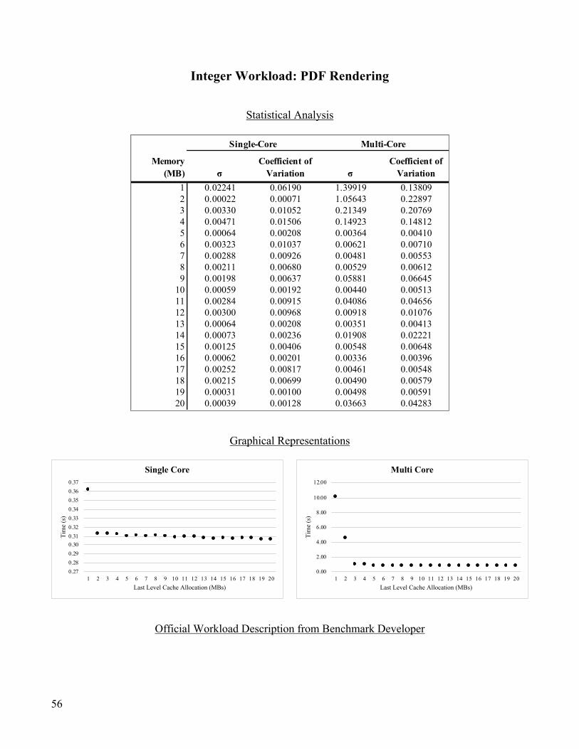
56

Integer Workload: PDF Rendering

Statistical Analysis

Graphical Representations

Official Workload Description from Benchmark Developer

Memory (MB) σ

Coefficient of Variation σ

Coefficient of Variation

1 0.02241 0.06190 1.39919 0.138092 0.00022 0.00071 1.05643 0.228973 0.00330 0.01052 0.21349 0.207694 0.00471 0.01506 0.14923 0.148125 0.00064 0.00208 0.00364 0.004106 0.00323 0.01037 0.00621 0.007107 0.00288 0.00926 0.00481 0.005538 0.00211 0.00680 0.00529 0.006129 0.00198 0.00637 0.05881 0.0664510 0.00059 0.00192 0.00440 0.0051311 0.00284 0.00915 0.04086 0.0465612 0.00300 0.00968 0.00918 0.0107613 0.00064 0.00208 0.00351 0.0041314 0.00073 0.00236 0.01908 0.0222115 0.00125 0.00406 0.00548 0.0064816 0.00062 0.00201 0.00336 0.0039617 0.00252 0.00817 0.00461 0.0054818 0.00215 0.00699 0.00490 0.0057919 0.00031 0.00100 0.00498 0.0059120 0.00039 0.00128 0.03663 0.04283

Single-Core Multi-Core

0.270.280.290.300.310.320.330.340.350.360.37

1 2 3 4 5 6 7 8 9 10 11 12 13 14 15 16 17 18 19 20

Tim

e (s

)

Last Level Cache Allocation (MBs)

Single Core

0.00

2.00

4.00

6.00

8.00

10.00

12.00

1 2 3 4 5 6 7 8 9 10 11 12 13 14 15 16 17 18 19 20

Tim

e (s

)

Last Level Cache Allocation (MBs)

Multi Core

57

The Portable Document Format (PDF) is a standard file format used to present and exchange documents independent of software or hardware. PDF files are used in numerous ways, from government documents and forms to e-books.

The PDF workload parses and renders a PDF map of Crater Lake National Park at 200dpi. The PDF workload uses the PDFium library (which is used by Google Chrome to display PDFs).

Practical Applications: How This Algorithm Is Used In Industry

The PDF is one of the most commonly used file formats, known to render the document the same

on any machine due to the file containing all information necessary to generate fonts, text, images, and

other elements of the intended layout. These documents can be viewed with built-in software that ships

with most computers, or with aftermarket software known as Adobe Acrobat Reader.

58

Integer Workload: Text Rendering

Statistical Analysis

Graphical Representations

Official Workload Description from Benchmark Developer

Memory (MB) σ

Coefficient of Variation σ

Coefficient of Variation

1 0.01970 0.25278 0.16368 0.243462 0.00058 0.01068 0.00832 0.034123 0.00015 0.00286 0.00260 0.011424 0.00108 0.02002 0.00129 0.005655 0.00151 0.02787 0.00170 0.007486 0.00254 0.04611 0.00175 0.007707 0.00113 0.02097 0.00190 0.008428 0.00232 0.04150 0.00182 0.008079 0.00268 0.04810 0.00419 0.0184710 0.00199 0.03569 0.00189 0.0084411 0.00174 0.03181 0.00697 0.0306412 0.00138 0.02520 0.00094 0.0041813 0.00107 0.01982 0.00074 0.0032614 0.00332 0.05957 0.00113 0.0049915 0.00203 0.03688 0.00219 0.0098216 0.00240 0.04333 0.00165 0.0073017 0.00169 0.03139 0.00233 0.0103818 0.00224 0.04068 0.00185 0.0082519 0.00185 0.03408 0.00162 0.0072320 0.00117 0.02174 0.00117 0.00521

Single-Core Multi-Core

0.000.01

0.020.03

0.040.050.06

0.070.08

0.09

1 2 3 4 5 6 7 8 9 10 11 12 13 14 15 16 17 18 19 20

Tim

e (s

)

Last Level Cache Allocation (MBs)

Single Core

0.00

0.10

0.20

0.30

0.40

0.50

0.60

0.70

0.80

1 2 3 4 5 6 7 8 9 10 11 12 13 14 15 16 17 18 19 20

Tim

e (s

)

Last Level Cache Allocation (MBs)

Multi Core

59

The Text Rendering workload parses a Markdown-formatted document and renders it as rich text to a bitmap. The Text Rendering workload uses the following libraries as part of the workload:

• GitHub Flavored Markdown, used to parse the Markdown document. • FreeType, used to render fonts. • ICU (International Components for Unicode), used for boundary analysis. The Text Rendering workload input file is 1721 words long and produces a bitmap

that is 1275 pixels by 9878 pixels in size.

Practical Applications: How This Algorithm Is Used In Industry

The text rendering in this algorithm is similar to that of an office suite / word processor (e.g.

Microsoft Word, Excel, PowerPoint, and Outlook). It reads a raw layout file, loads fonts, and generates

the printable layout page.

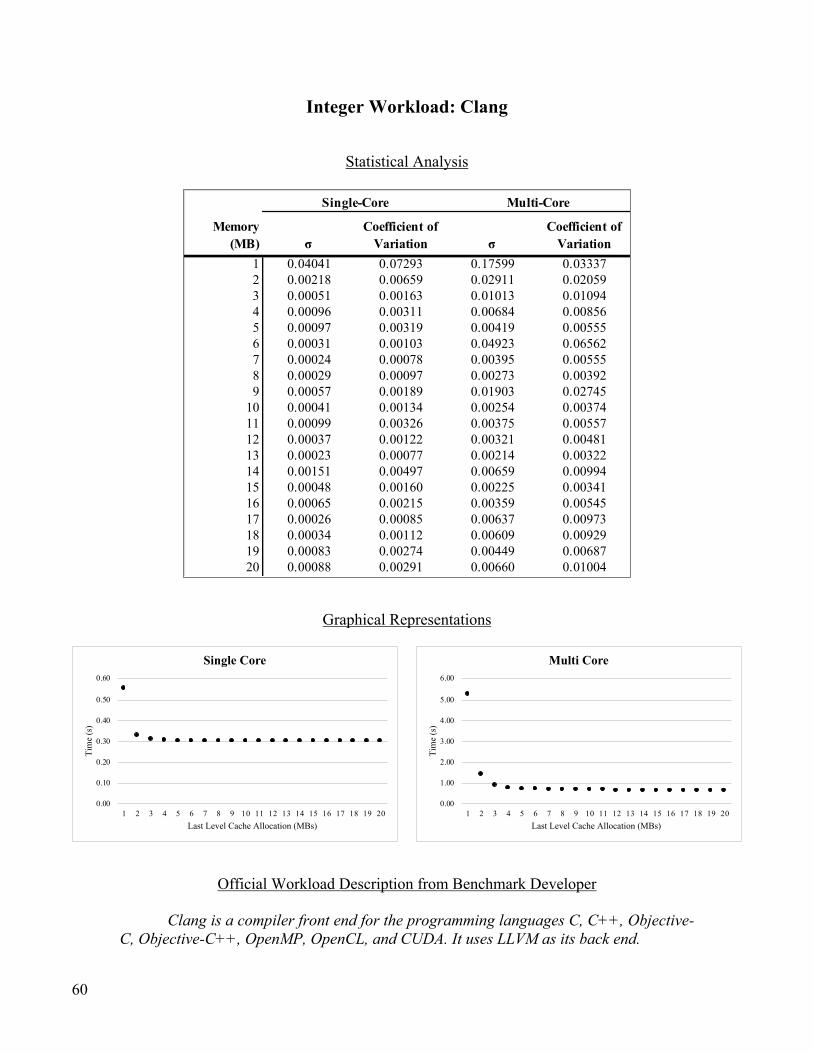
60

Integer Workload: Clang

Statistical Analysis

Graphical Representations

Official Workload Description from Benchmark Developer

Clang is a compiler front end for the programming languages C, C++, Objective-C, Objective-C++, OpenMP, OpenCL, and CUDA. It uses LLVM as its back end.

Memory (MB) σ

Coefficient of Variation σ

Coefficient of Variation

1 0.04041 0.07293 0.17599 0.033372 0.00218 0.00659 0.02911 0.020593 0.00051 0.00163 0.01013 0.010944 0.00096 0.00311 0.00684 0.008565 0.00097 0.00319 0.00419 0.005556 0.00031 0.00103 0.04923 0.065627 0.00024 0.00078 0.00395 0.005558 0.00029 0.00097 0.00273 0.003929 0.00057 0.00189 0.01903 0.0274510 0.00041 0.00134 0.00254 0.0037411 0.00099 0.00326 0.00375 0.0055712 0.00037 0.00122 0.00321 0.0048113 0.00023 0.00077 0.00214 0.0032214 0.00151 0.00497 0.00659 0.0099415 0.00048 0.00160 0.00225 0.0034116 0.00065 0.00215 0.00359 0.0054517 0.00026 0.00085 0.00637 0.0097318 0.00034 0.00112 0.00609 0.0092919 0.00083 0.00274 0.00449 0.0068720 0.00088 0.00291 0.00660 0.01004

Single-Core Multi-Core

0.00

0.10

0.20

0.30

0.40

0.50

0.60

1 2 3 4 5 6 7 8 9 10 11 12 13 14 15 16 17 18 19 20

Tim

e (s

)

Last Level Cache Allocation (MBs)

Single Core

0.00

1.00

2.00

3.00

4.00

5.00

6.00

1 2 3 4 5 6 7 8 9 10 11 12 13 14 15 16 17 18 19 20

Tim

e (s

)

Last Level Cache Allocation (MBs)

Multi Core

61

The Clang workload compiles a 1,094 line C source file (of which 729 lines are code). The workload uses AArch64 as the target architecture for code generation.

Practical Applications: How This Algorithm Is Used In Industry

This workload represents a more developer-facing feature, whereby raw code is transformed into

computer code through a process known as “compilation.” Most programs are already compiled before

the user receives them, so this is likely not a workload that the consumer will interact with.

62

Integer Workload: Camera

Statistical Analysis

Graphical Representations

Official Workload Description from Benchmark Developer

Camera replicates a photo sharing application like Instagram. Camera merges several steps into one workload:

Memory (MB) σ

Coefficient of Variation σ

Coefficient of Variation

1 0.00963 0.06764 0.05078 0.028452 0.00398 0.03222 0.02123 0.018143 0.00422 0.03403 0.01691 0.018724 0.00329 0.02738 0.01695 0.025505 0.00354 0.02900 0.02247 0.044586 0.00396 0.03248 0.02077 0.051867 0.00192 0.01606 0.00890 0.025018 0.00368 0.03028 0.00163 0.004719 0.00299 0.02481 0.00179 0.0052510 0.00292 0.02418 0.00235 0.0069311 0.00365 0.03005 0.00136 0.0040112 0.00275 0.02294 0.00055 0.0016313 0.00131 0.01094 0.00056 0.0016714 0.00281 0.02340 0.00141 0.0041715 0.00095 0.00769 0.00148 0.0043816 0.00345 0.02854 0.00139 0.0041317 0.00079 0.00665 0.00177 0.0052518 0.00089 0.00746 0.00062 0.0018519 0.00258 0.02147 0.00090 0.0026820 0.00245 0.02039 0.00126 0.00376

Single-Core Multi-Core

0.00

0.02

0.04

0.06

0.08

0.10

0.12

0.14

0.16

1 2 3 4 5 6 7 8 9 10 11 12 13 14 15 16 17 18 19 20

Tim

e (s

)

Last Level Cache Allocation (MBs)

Single Core

0.000.200.400.600.801.001.201.401.601.802.00

1 2 3 4 5 6 7 8 9 10 11 12 13 14 15 16 17 18 19 20

Tim

e (s

)

Last Level Cache Allocation (MBs)

Multi Core

63

• SHA2 checksum generation • JSON parsing • Image compositing • Image filters (gaussian blur, contrast) • Image resizing (thumbnail generation) • SQLite (SELECT images to be processed) All steps run on the CPU and are not accelerated by the GPU.

Practical Applications: How This Algorithm Is Used In Industry

This is a workload that represents the browsing and exporting of photos, rather than the creation

of the individual photo. Any time that a photo is displayed on a computer, it likely went through a process

similar to this (e.g. when viewing your photos in Apple’s Photos app or Google Photos). This is also true

for photo-browsing programs such as Snapchat, Instagram, Facebook, and Twitter.

64

Floating Point Workload: N-Body Physics

Statistical Analysis

Graphical Representations

Official Workload Description from Benchmark Developer

The N-Body Physics workload computes a 3D gravitation simulation using the Barnes-Hut method. To compute the exact gravitational force acting on a particular body

Memory (MB) σ

Coefficient of Variation σ

Coefficient of Variation

1 0.01716 0.00890 0.12760 0.319382 0.02949 0.02289 0.00092 0.004803 0.02578 0.02556 0.00229 0.014644 0.01763 0.01995 0.00278 0.020125 0.03299 0.04127 0.00088 0.006966 0.01054 0.01393 0.00453 0.037177 0.00560 0.00762 0.00065 0.005698 0.00220 0.00303 0.00046 0.004159 0.00105 0.00145 0.00027 0.0024010 0.00072 0.00101 0.00060 0.0055211 0.00270 0.00378 0.00041 0.0037212 0.00201 0.00281 0.00023 0.0020913 0.00054 0.00075 0.00048 0.0043914 0.00285 0.00398 0.00103 0.0093915 0.00167 0.00235 0.00035 0.0032116 0.00254 0.00356 0.00115 0.0105317 0.00153 0.00213 0.00064 0.0058418 0.00072 0.00100 0.00046 0.0041819 0.02488 0.03429 0.00057 0.0052420 0.00122 0.00171 0.00045 0.00414

Single-Core Multi-Core

0.00

0.50

1.00

1.50

2.00

2.50

1 2 3 4 5 6 7 8 9 10 11 12 13 14 15 16 17 18 19 20

Tim

e (s

)

Last Level Cache Allocation (MBs)

Single Core

0.000.05

0.100.15

0.200.250.30

0.350.40

0.45

1 2 3 4 5 6 7 8 9 10 11 12 13 14 15 16 17 18 19 20

Tim

e (s

)

Last Level Cache Allocation (MBs)

Multi Core

65

x in a field of N bodies requires N − 1 force computations. The Barnes-Hut method reduces the number of force computations by approximating as a single body any tight cluster of bodies that is far away from x. It does this efficiently by dividing the space into octants — eight cubes of equal size — and recursively subdividing each octant into octants, forming a tree, until each leaf octant contains exactly one body. This recursive subdivision of the space requires floating point operations and non-contiguous memory accesses.

The N-Body Physics workload operates on 16,384 bodies arranged in a “flat” galaxy with a massive black hole in its centre.

Practical Applications: How This Algorithm Is Used In Industry

The physics calculations used in this benchmark are used to calculate the scrolling inertia and

momentum in any graphical user interface that supports “natural scrolling.” Put another way, when you

scroll (either on a trackpad or with your finger on a touchscreen), notice how the page keep scrolling when

you remove your finger. The duration of the motion differs based on the speed and motion with which

you input direction on the screen or trackpad. The current velocity of the scroll is then measured and

tapered to 0 meters per second based on a friction constant set by the operating system vendor. Without

this, the scrolling would appear “choppy.”

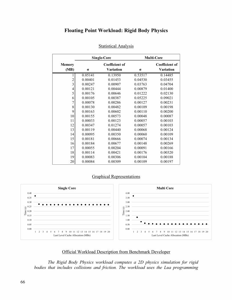
66

Floating Point Workload: Rigid Body Physics

Statistical Analysis

Graphical Representations

Official Workload Description from Benchmark Developer

The Rigid Body Physics workload computes a 2D physics simulation for rigid bodies that includes collisions and friction. The workload uses the Lua programming

Memory (MB) σ

Coefficient of Variation σ

Coefficient of Variation

1 0.05141 0.13950 0.53517 0.144852 0.00401 0.01453 0.04530 0.034553 0.00247 0.00907 0.03763 0.047044 0.00121 0.00444 0.00879 0.014005 0.00176 0.00646 0.01222 0.021306 0.00105 0.00387 0.05225 0.090217 0.00078 0.00286 0.00127 0.002318 0.00130 0.00482 0.00109 0.001989 0.00163 0.00602 0.00110 0.0020010 0.00155 0.00573 0.00048 0.0008711 0.00033 0.00123 0.00057 0.0010312 0.00347 0.01274 0.00057 0.0010313 0.00119 0.00440 0.00068 0.0012414 0.00095 0.00350 0.00060 0.0010915 0.00181 0.00666 0.00074 0.0013416 0.00184 0.00677 0.00148 0.0026917 0.00055 0.00204 0.00091 0.0016618 0.00114 0.00421 0.00176 0.0032019 0.00083 0.00306 0.00104 0.0018820 0.00084 0.00309 0.00109 0.00197

Single-Core Multi-Core

0.00

0.05

0.10

0.15

0.20

0.25

0.30

0.35

0.40

1 2 3 4 5 6 7 8 9 10 11 12 13 14 15 16 17 18 19 20

Tim

e (s

)

Last Level Cache Allocation (MBs)

Single Core

0.00

0.50

1.00

1.50

2.00

2.50

3.00

3.50

4.00

1 2 3 4 5 6 7 8 9 10 11 12 13 14 15 16 17 18 19 20

Tim

e (s

)

Last Level Cache Allocation (MBs)

Multi Core

67

language to initialize and manage the physics simulation, and uses the Box2D physics library to perform the actual physics calculations.

Practical Applications: How This Algorithm Is Used In Industry

Like the previous example, this physics simulation is used to determine the “elastic” nature of the

scrolling, whereby the user scrolls past the end of a page and thus the page border “collides” with the item

it is next to providing a certain amount of negative force and slightly bouncing the scroll in the opposite

direction. Without this, scrolling would abruptly stop when a user reached the end of a page.

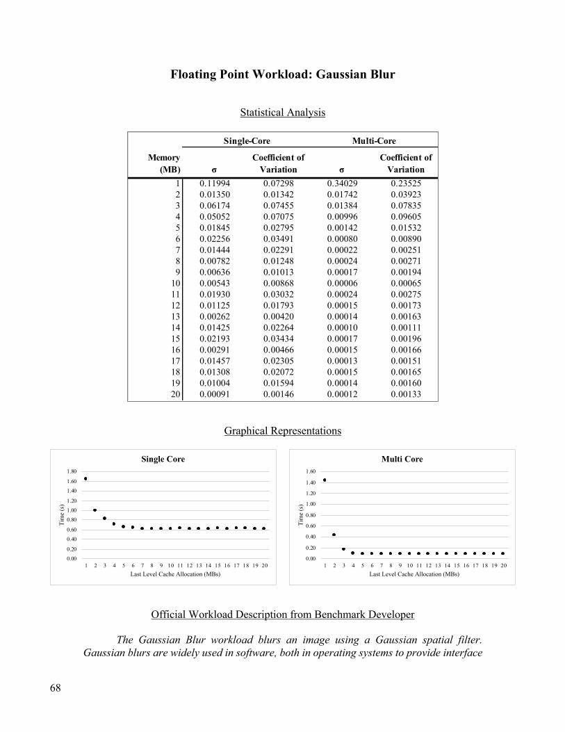
68

Floating Point Workload: Gaussian Blur

Statistical Analysis

Graphical Representations

Official Workload Description from Benchmark Developer

The Gaussian Blur workload blurs an image using a Gaussian spatial filter. Gaussian blurs are widely used in software, both in operating systems to provide interface

Memory (MB) σ

Coefficient of Variation σ

Coefficient of Variation

1 0.11994 0.07298 0.34029 0.235252 0.01350 0.01342 0.01742 0.039233 0.06174 0.07455 0.01384 0.078354 0.05052 0.07075 0.00996 0.096055 0.01845 0.02795 0.00142 0.015326 0.02256 0.03491 0.00080 0.008907 0.01444 0.02291 0.00022 0.002518 0.00782 0.01248 0.00024 0.002719 0.00636 0.01013 0.00017 0.0019410 0.00543 0.00868 0.00006 0.0006511 0.01930 0.03032 0.00024 0.0027512 0.01125 0.01793 0.00015 0.0017313 0.00262 0.00420 0.00014 0.0016314 0.01425 0.02264 0.00010 0.0011115 0.02193 0.03434 0.00017 0.0019616 0.00291 0.00466 0.00015 0.0016617 0.01457 0.02305 0.00013 0.0015118 0.01308 0.02072 0.00015 0.0016519 0.01004 0.01594 0.00014 0.0016020 0.00091 0.00146 0.00012 0.00133

Single-Core Multi-Core

0.000.20

0.400.60

0.801.001.20

1.401.60

1.80

1 2 3 4 5 6 7 8 9 10 11 12 13 14 15 16 17 18 19 20

Tim

e (s

)

Last Level Cache Allocation (MBs)

Single Core

0.00

0.20

0.40

0.60

0.80

1.00

1.20

1.40

1.60

1 2 3 4 5 6 7 8 9 10 11 12 13 14 15 16 17 18 19 20

Tim

e (s

)

Last Level Cache Allocation (MBs)

Multi Core

69

effects, and in image editing software to reduce detail and noise in an image. Gaussian blurs are also used in computer vision applications to enhance image structures at different scales.

The Gaussian Blur workload blurs an 24 megapixel image using a Gaussian spatial filter. While the Gaussian blur implementation supports an arbitrary sigma, the workload uses a fixed sigma of 3.0f. This sigma translates into a filter diameter of 25 pixels by 25 pixels.

Practical Applications: How This Algorithm Is Used In Industry

This algorithm is used by the windowing system on many operating systems (e.g. Windows 7,

macOS, and iOS). These operating systems construct the windows using a blur of the background of the

windows underneath, creating a translucency-like effect. Although you may have not noticed this, it is

consuming computing resources every time any window changes position on the screen. A computer with

three 4K monitors (effectively 8.5 megapixels each) would effectively be doing the same amount of

computation as done in this workload.

70

Floating Point Workload: Face Detection

Statistical Analysis

Graphical Representations

Official Workload Description from Benchmark Developer

Memory (MB) σ

Coefficient of Variation σ

Coefficient of Variation

1 0.00684 0.03729 0.99541 0.512522 0.00389 0.02363 0.03669 0.079563 0.01026 0.06127 0.00319 0.008004 0.00425 0.02593 0.00152 0.003965 0.00481 0.02932 0.00057 0.001526 0.00368 0.02222 0.00056 0.001507 0.00224 0.01368 0.00028 0.000768 0.00355 0.02187 0.00080 0.002169 0.00126 0.00781 0.00055 0.0015010 0.00074 0.00463 0.00035 0.0009611 0.00433 0.02614 0.00071 0.0019312 0.00712 0.04265 0.00055 0.0015013 0.00310 0.01874 0.00097 0.0026614 0.00164 0.01021 0.00097 0.0026615 0.00365 0.02185 0.00082 0.0022316 0.00184 0.01132 0.00083 0.0022917 0.00523 0.03190 0.00253 0.0069318 0.00470 0.02873 0.00003 0.0000919 0.00405 0.02505 0.00213 0.0058320 0.00158 0.00983 0.00147 0.00403

Single-Core Multi-Core

0.150.15

0.160.16

0.170.170.18

0.180.19

0.19

1 2 3 4 5 6 7 8 9 10 11 12 13 14 15 16 17 18 19 20

Tim

e (s

)

Last Level Cache Allocation (MBs)

Single Core

0.00

0.50

1.00

1.50

2.00

2.50

1 2 3 4 5 6 7 8 9 10 11 12 13 14 15 16 17 18 19 20

Tim

e (s

)

Last Level Cache Allocation (MBs)

Multi Core

71

Face detection is a computer vision technique that identifies human faces in digital images. One application of face detection is in photography, where camera applications use face detection for autofocus.

The Face Detection workload uses the algorithm presented in “Rapid Object Detection using a Boosted Cascade of Simple Features” (2001) by Viola and Jones. The algorithm can produce multiple boxes for each face. These boxes are reduced to a single box using non-maximum suppression.

Practical Applications: How This Algorithm Is Used In Industry

Photo and video cataloging software (e.g. Apple’s Photos App, Google Photos) scans your

multimedia to detect the presence of faces. Although this is slightly different from image classification

algorithm explained later in this paper, it is able to search for only the face objects. Once found, the

algorithm can be combined with a standard Machine Learning algorithm, such as the one later in this

paper, to form a collection of images containing an individual’s face.

72

Floating Point Workload: Horizon Detection

Statistical Analysis

Graphical Representations

Official Workload Description from Benchmark Developer

The Horizon Detection workload searches for the horizon line in an image. If the horizon line is found, the workload rotates the image to make the horizon line level.

Memory (MB) σ

Coefficient of Variation σ

Coefficient of Variation

1 0.00210 0.00429 1.32555 0.392132 0.00170 0.00362 0.02206 0.014633 0.00599 0.01263 0.00395 0.002864 0.00123 0.00263 0.00385 0.002835 0.00236 0.00505 0.00300 0.002236 0.00456 0.00975 0.00087 0.000657 0.00210 0.00449 0.00156 0.001178 0.00471 0.01007 0.00273 0.002069 0.00484 0.01035 0.00204 0.0015410 0.00220 0.00472 0.00301 0.0022811 0.00443 0.00946 0.00185 0.0014112 0.00451 0.00968 0.00131 0.0010013 0.00199 0.00428 0.00349 0.0026514 0.00423 0.00910 0.00257 0.0019515 0.00136 0.00294 0.00390 0.0029616 0.00214 0.00461 0.00174 0.0013217 0.00469 0.01010 0.00701 0.0053318 0.00494 0.01061 0.00207 0.0015819 0.00495 0.01065 0.00106 0.0008020 0.00144 0.00313 0.00314 0.00239

Single-Core Multi-Core

0.450.450.460.460.470.470.480.480.490.490.50

1 2 3 4 5 6 7 8 9 10 11 12 13 14 15 16 17 18 19 20

Tim

e (s

)

Last Level Cache Allocation (MBs)

Single Core

0.00

0.50

1.00

1.50

2.00

2.50

3.00

3.50

4.00

1 2 3 4 5 6 7 8 9 10 11 12 13 14 15 16 17 18 19 20

Tim

e (s

)

Last Level Cache Allocation (MBs)

Multi Core

73

The workload first applies a Canny edge detector to the image to reduce details, then detects lines in the image using the Hough transform, and then picks the line with the maximum score as the horizon. The workload rotates the image so the horizon line is level in the image.

Practical Applications: How This Algorithm Is Used In Industry

This algorithm can be used to determine the proper rotation of a photo on modern cameras.

Combined with gyroscopic sensors, the system searches for the earth’s horizon in the photo and once

found is able to rotate the photo accordingly so that when viewed, it is the correct orientation.

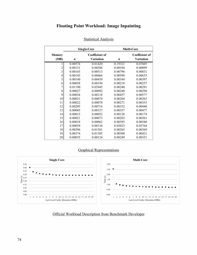
74

Floating Point Workload: Image Inpainting

Statistical Analysis

Graphical Representations

Official Workload Description from Benchmark Developer

Memory (MB) σ

Coefficient of Variation σ

Coefficient of Variation

1 0.00574 0.01420 0.19321 0.076052 0.00131 0.00386 0.00104 0.000993 0.00165 0.00513 0.00796 0.008314 0.00145 0.00466 0.00590 0.006535 0.00140 0.00459 0.00344 0.003976 0.00058 0.00194 0.00218 0.002577 0.01190 0.03945 0.00240 0.002918 0.00027 0.00092 0.00240 0.002989 0.00034 0.00118 0.00457 0.0057710 0.00021 0.00074 0.00204 0.0026311 0.00022 0.00078 0.00271 0.0035512 0.00205 0.00714 0.00332 0.0044013 0.00045 0.00157 0.00357 0.0047714 0.00015 0.00052 0.00128 0.0017415 0.00021 0.00073 0.00265 0.0036116 0.00018 0.00062 0.00393 0.0054017 0.00039 0.00136 0.02023 0.0276418 0.00396 0.01381 0.00265 0.0036919 0.00374 0.01305 0.00300 0.0042120 0.00035 0.00124 0.00249 0.00351

Single-Core Multi-Core

0.000.05

0.100.15

0.200.250.30

0.350.40

0.45

1 2 3 4 5 6 7 8 9 10 11 12 13 14 15 16 17 18 19 20

Tim

e (s

)

Last Level Cache Allocation (MBs)

Single Core

0.00

0.50

1.00

1.50

2.00

2.50

3.00

1 2 3 4 5 6 7 8 9 10 11 12 13 14 15 16 17 18 19 20

Tim

e (s

)

Last Level Cache Allocation (MBs)

Multi Core

75

The Image Inpainting workload takes an input image with an undesirable region (indicated via a mask image) and uses an inpainting scheme to reconstruct the region using data from outside the undesirable region.

The Image Inpainting workload operates on 1 megapixel images.

Practical Applications: How This Algorithm Is Used In Industry

Modern cameras (e.g. Apple’s iPhone XS) make use of image compositing features to construct

an image that is “better” than the image actually captured by removing blemishes, red eyes, and blurry

parts of the scene. Once the processor receives the raw image file, it analyzes it to find the issue regions

of the photograph, composites a mask, and “repaints” the photo to how the system believes it should look.

76

Floating Point Workload: HDR

Statistical Analysis

Graphical Representations

Official Workload Description from Benchmark Developer

The HDR workload takes four standard dynamic range (SDR) images and produces a high dynamic range (HDR) image.

Memory (MB) σ

Coefficient of Variation σ

Coefficient of Variation

1 0.00666 0.00641 4.60725 0.558062 0.00591 0.00592 1.02560 0.330843 0.00086 0.00087 0.00664 0.002624 0.00205 0.00206 0.00424 0.001705 0.00296 0.00298 0.01091 0.004416 0.00360 0.00362 0.01010 0.004117 0.00816 0.00820 0.01052 0.004308 0.00203 0.00205 0.01318 0.005409 0.00374 0.00377 0.00833 0.0034110 0.01013 0.01019 0.00484 0.0019911 0.00429 0.00429 0.00562 0.0023112 0.00189 0.00190 0.00920 0.0037813 0.00201 0.00203 0.00516 0.0021314 0.00375 0.00379 0.00999 0.0041215 0.00569 0.00573 0.00667 0.0027616 0.00342 0.00345 0.00209 0.0008617 0.00219 0.00221 0.05482 0.0225018 0.00194 0.00196 0.00306 0.0012719 0.00571 0.00575 0.00631 0.0026120 0.00017 0.00017 0.00661 0.00274

Single-Core Multi-Core

0.960.97

0.980.99

1.001.011.02

1.031.04

1.05

1 2 3 4 5 6 7 8 9 10 11 12 13 14 15 16 17 18 19 20

Tim

e (s

)

Last Level Cache Allocation (MBs)

Single Core

0.001.00

2.003.00

4.005.006.00

7.008.00

9.00

1 2 3 4 5 6 7 8 9 10 11 12 13 14 15 16 17 18 19 20

Tim

e (s

)

Last Level Cache Allocation (MBs)

Multi Core

77

The HDR workload uses the algorithm described in the paper, "Dynamic Range Reduction inspired by Photoreceptor Physiology" by Reinhard and Devlin, and produces superior images as compared to the tone mapping algorithm in Geekbench 4.

Practical Applications: How This Algorithm Is Used In Industry

This algorithm has been in wide commercial use since Apple released the iPhone 4 in 2010. In

scenes with a difference between the lightest and darkest parts, the image can either be either too bright

or dark to see detail. To produce a better photo, the camera combines a high-contrast photo, low-contrast

photo and normal contrast-photo of the scene together to form one composite image that keeps a more

consistent final image where the details are still visible without dampening the dark or light parts of the

image.

78

Floating Point Workload: Ray Tracing

Statistical Analysis

Graphical Representations

Official Workload Description from Benchmark Developer

Ray tracing is a rendering technique. Ray tracing generates an image by tracing the path of light through an image plane and simulating the effects of its encounters with

Memory (MB) σ

Coefficient of Variation σ

Coefficient of Variation

1 0.02749 0.09732 0.25329 0.086492 0.00070 0.00644 0.03319 0.175613 0.00143 0.01376 0.00466 0.045684 0.00036 0.00354 0.00175 0.018735 0.00024 0.00231 0.00123 0.013436 0.00058 0.00568 0.00081 0.008927 0.00039 0.00387 0.00064 0.007058 0.00054 0.00535 0.00112 0.012369 0.00057 0.00570 0.00079 0.0087710 0.00033 0.00329 0.00165 0.0183511 0.00042 0.00415 0.00059 0.0065212 0.00055 0.00547 0.00061 0.0066113 0.00035 0.00350 0.00154 0.0167214 0.00039 0.00391 0.00093 0.0103215 0.00026 0.00261 0.00045 0.0050216 0.00055 0.00546 0.00057 0.0063817 0.00054 0.00535 0.00170 0.0187518 0.00045 0.00454 0.00101 0.0111819 0.00049 0.00492 0.00091 0.0101720 0.00044 0.00438 0.00077 0.00856

Single-Core Multi-Core

0.00

0.05

0.10

0.15

0.20

0.25

0.30

1 2 3 4 5 6 7 8 9 10 11 12 13 14 15 16 17 18 19 20

Tim

e (s

)

Last Level Cache Allocation (MBs)

Single Core

0.00

0.50

1.00

1.50

2.00

2.50

3.00

3.50

1 2 3 4 5 6 7 8 9 10 11 12 13 14 15 16 17 18 19 20

Tim

e (s

)

Last Level Cache Allocation (MBs)

Multi Core

79

virtual objects. This method is capable of producing high-quality images, but these images come at a high computational cost.

The Ray Tracing workload uses a k-d tree, a space-partitioning data structure, to accelerate the ray intersection calculations.

The Ray Tracing workload operates on a scene with 3,608 textured triangles. The rendered image is 768 pixels by 768 pixels.

Practical Applications: How This Algorithm Is Used In Industry

This algorithm forms the basis for many video games, which rely on drawing textures and shapes

through rays. Nearly every video game with a 3D perspective makes use of a Ray Tracing algorithm to

render the scene. Generally, the faster the rays can be drawn, the more frames can be displayed and the

better the game playing experience for the user.

80

Floating Point Workload: Structure from Motion

Statistical Analysis

Graphical Representations

Official Workload Description from Benchmark Developer

Augmented reality (AR) systems add computer-generated graphics to real-world scenes. The systems must have an understanding of the geometry of the real-world scene

Memory (MB) σ

Coefficient of Variation σ

Coefficient of Variation

1 0.10231 0.07079 2.56771 0.141622 0.01654 0.01345 0.14101 0.015403 0.00696 0.00571 0.06024 0.009224 0.00332 0.00273 0.05535 0.012405 0.00738 0.00605 0.06836 0.018976 0.00555 0.00457 0.02674 0.008337 0.00447 0.00368 0.01425 0.004618 0.00240 0.00198 0.02202 0.007189 0.00272 0.00224 0.01282 0.0042010 0.00116 0.00095 0.00874 0.0028611 0.00708 0.00579 0.00699 0.0023012 0.00552 0.00453 0.00591 0.0019513 0.00747 0.00610 0.05887 0.0192214 0.00745 0.00611 0.00546 0.0018015 0.00405 0.00333 0.00593 0.0019516 0.01028 0.00842 0.00610 0.0020117 0.00407 0.00335 0.00435 0.0014318 0.00341 0.00280 0.00556 0.0018319 0.00596 0.00489 0.07022 0.0228920 0.00458 0.00377 0.00574 0.00189

Single-Core Multi-Core

1.051.10

1.151.20

1.251.301.35

1.401.45

1.50

1 2 3 4 5 6 7 8 9 10 11 12 13 14 15 16 17 18 19 20

Tim

e (s

)

Last Level Cache Allocation (MBs)

Single Core

0.002.004.006.008.00

10.0012.0014.0016.0018.0020.00

1 2 3 4 5 6 7 8 9 10 11 12 13 14 15 16 17 18 19 20

Tim

e (s

)

Last Level Cache Allocation (MBs)

Multi Core

81

in order to properly integrate the computer-generated graphics. One approach to calculating the geometry is through Structure from Motion (SfM) algorithms.

The Structure from Motion workload takes two 2D images of the same scene and constructs an estimate of the 3D coordinates of the points visible in both images.

Practical Applications: How This Algorithm Is Used In Industry

This algorithm is similar in nature to photo creation on devices with multiple cameras (e.g. Apple

iPhone 11’s 3 cameras in “Portrait Mode,” Google Pixel 4’s 3 cameras). Multiple photos are captured

simultaneously, and the system performs an analysis to determine the depth of certain objects in the frame.

Once these coordinates and objects are identified, special effects such as a background blur can be applied

to the photos.

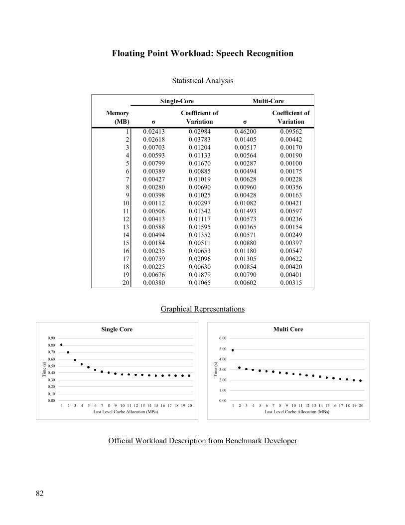
82

Floating Point Workload: Speech Recognition

Statistical Analysis

Graphical Representations

Official Workload Description from Benchmark Developer

Memory (MB) σ

Coefficient of Variation σ

Coefficient of Variation

1 0.02413 0.02984 0.46200 0.095622 0.02618 0.03783 0.01405 0.004423 0.00703 0.01204 0.00517 0.001704 0.00593 0.01133 0.00564 0.001905 0.00799 0.01670 0.00287 0.001006 0.00389 0.00885 0.00494 0.001757 0.00427 0.01019 0.00628 0.002288 0.00280 0.00690 0.00960 0.003569 0.00398 0.01025 0.00428 0.0016310 0.00112 0.00297 0.01082 0.0042111 0.00506 0.01342 0.01493 0.0059712 0.00413 0.01117 0.00573 0.0023613 0.00588 0.01595 0.00365 0.0015414 0.00494 0.01352 0.00571 0.0024915 0.00184 0.00511 0.00880 0.0039716 0.00235 0.00653 0.01180 0.0054717 0.00759 0.02096 0.01305 0.0062218 0.00225 0.00630 0.00854 0.0042019 0.00676 0.01879 0.00790 0.0040120 0.00380 0.01065 0.00602 0.00315

Single-Core Multi-Core

0.000.10

0.200.30

0.400.500.60

0.700.80

0.90

1 2 3 4 5 6 7 8 9 10 11 12 13 14 15 16 17 18 19 20

Tim

e (s

)

Last Level Cache Allocation (MBs)

Single Core

0.00

1.00

2.00

3.00

4.00

5.00

6.00

1 2 3 4 5 6 7 8 9 10 11 12 13 14 15 16 17 18 19 20

Tim

e (s

)

Last Level Cache Allocation (MBs)

Multi Core

83

The Speech Recognition workload performs recognition of arbitrary English speech using PocketSphinx, a widely used library that uses HMM (Hidden Markov Models).

Using speech to interact with smartphones is becoming more popular with the introduction of Siri, Google Assistant, and Cortana, and this workload tests how quickly a device can process sound and recognize the words that are being spoken.

Practical Applications: How This Algorithm Is Used In Industry

This algorithm is the basis for digital assistants (e.g. Apple’s Siri, Google Assistant, Amazon

Alexa, and Microsoft Cortana) and speech-to-text recognition. It uses an input of an audio file and

performs an analysis of the data to determine a text transcription of what was spoken.

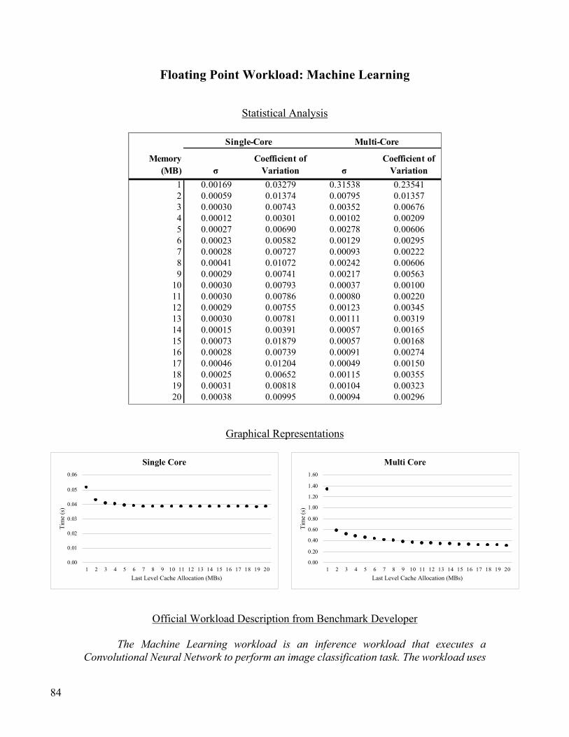
84

Floating Point Workload: Machine Learning

Statistical Analysis

Graphical Representations

Official Workload Description from Benchmark Developer

The Machine Learning workload is an inference workload that executes a Convolutional Neural Network to perform an image classification task. The workload uses

Memory (MB) σ

Coefficient of Variation σ

Coefficient of Variation

1 0.00169 0.03279 0.31538 0.235412 0.00059 0.01374 0.00795 0.013573 0.00030 0.00743 0.00352 0.006764 0.00012 0.00301 0.00102 0.002095 0.00027 0.00690 0.00278 0.006066 0.00023 0.00582 0.00129 0.002957 0.00028 0.00727 0.00093 0.002228 0.00041 0.01072 0.00242 0.006069 0.00029 0.00741 0.00217 0.0056310 0.00030 0.00793 0.00037 0.0010011 0.00030 0.00786 0.00080 0.0022012 0.00029 0.00755 0.00123 0.0034513 0.00030 0.00781 0.00111 0.0031914 0.00015 0.00391 0.00057 0.0016515 0.00073 0.01879 0.00057 0.0016816 0.00028 0.00739 0.00091 0.0027417 0.00046 0.01204 0.00049 0.0015018 0.00025 0.00652 0.00115 0.0035519 0.00031 0.00818 0.00104 0.0032320 0.00038 0.00995 0.00094 0.00296

Single-Core Multi-Core

0.00

0.01

0.02

0.03

0.04

0.05

0.06

1 2 3 4 5 6 7 8 9 10 11 12 13 14 15 16 17 18 19 20

Tim

e (s

)

Last Level Cache Allocation (MBs)

Single Core

0.00

0.20

0.40

0.60

0.80

1.00

1.20

1.40

1.60

1 2 3 4 5 6 7 8 9 10 11 12 13 14 15 16 17 18 19 20

Tim

e (s

)

Last Level Cache Allocation (MBs)

Multi Core

85

MobileNet v1 with an alpha of 1.0 and an input image size of 224 pixels by 224 pixels. The model was trained on the ImageNet47 dataset.

Practical Applications: How This Algorithm Is Used In Industry

Photo and video cataloging software (e.g. Apple’s Photos App, Google Photos) scans your

multimedia to perform image classification. This type of computer vision determines the presence of

objects such as inanimate items, animals, and persons within a media file. Note, this is different from the

earlier-described Machine Learning algorithm which performs facial recognition as this algorithm is

merely looking to see whether a human is in a media file, not to see whether a the human is a specific

person. This algorithm can be run after the face detection algorithm to determine who is in a photograph

based on other images of faces that are already known to the system.

47 The dataset is available at: http://www.image-net.org and contains words associated with images that are used to

train a Machine Learning algorithm.

86

References

Aggarwal, Gagan, Feldman, Jon, and Muthukrishnan, S. “Bidding to the Top: VCG and Equilibria of Position-Based Auctions” (2006) Google, Inc.

Aggarwal, Gagan, Goel, Ashish, and Motwani, Rajeev. “Truthful Auctions for Pricing Search Keywords.” (2006). Stanford University Departments of Computer Science, Management Science, and Engineering.

Chun, Brent, and Culler, David, “User-centric Performance Analysis of Market-based Cluster Batch

Schedulers” (2002). The University of California at Berkeley Computer Science Division. Clarke, Edward H. “Multipart Pricing of Public Goods.” Public Choice 11 (1971): 17-33.

http://www.jstor.org/stable/30022651.

Connolly, Michelle and Kwerel, Evan, “Economics at the Federal Communications Commission: 2006- 2007” (2007). Federal Communications Commission and Duke University Department of Economics.

Edelman, Benjamin, Ostrovsky, Michael, and Schwartz, Michael, “Internet Advertising and the Generalized Second-Price Auction: Selling Billions of Dollars Worth of Keywords” (2005). Harvard University Department of Economics, Stanford University Graduate School of Business.

Fan, Songchun, Zahedi, Seyed, and Lee, Benjamin, “The Computational Sprinting Game” (2016). Duke University Departments of Electrical Engineering and Computer Sciences.

Fan, Songchun, Zahedi, Seyed, and Lee, Benjamin, “Managing Heterogeneous Datacenters with Tokens” (2018). Google, L.L.C. and Duke University Departments of Electrical Engineering and Computer Sciences.

Groves, Theodore. “Incentives in Teams.” Econometrica 41, no. 4 (1973): 617-31. doi:10.2307/1914085.

Kuwabara, Kazuhiro et all, “An Equilibratory Market-Based Approach for Distributed Resource Allocation and Its Applications to Communication Network Control” (1995). NTT Communication Science Laboratories.

Mahdian, Mohammad, Nazerzadeh, and Saberi, Amin. “Allocating Online Advertisement Space with Unreliable Estimates” (2007). Yahoo! Inc, and Stanford University.

Silberschatz, Abraham, Greg Gagne, and Peter B. Galvin. Operating System Concepts, 8th Edition (2008). John Wiley & Sons.

Vickrey, William. “Counterspeculation, Auctions, and Competitive Sealed Tenders.” The Journal of Finance 16, no. 1 (1961): 8-37. doi:10.2307/2977633.

87

Zahedi, Seyed, and Lee, Benjamin, “REF: Resource Elasticity Fairness with Sharing Incentives for Multiprocessors” (2014). Duke University Departments of Electrical and Computer Engineering and Computer Science.

Zahedi, Seyed, Llull, Qiuyun, and Lee, Benjamin, “Amdahl’s Law in the Datacenter Era: A Market for

Fair Processor Allocation” (2018). VMware, Inc. and Duke University Departments of Electrical Engineering and Computer Sciences.