A Semantic Analysis of Key Management Protocolsfor Wireless Sensor NetworksI

Damiano Macedonio, Massimo Merro

Dipartimento di Informatica, Universita degli Studi di Verona, Italy

Abstract

Gorrieri and Martinelli’s timed Generalized Non-Deducibility on Compositions (tGNDC) schema is a well-knowngeneral framework for the formal verification of security protocols in a concurrent scenario. We generalise the tGNDCschema to verify wireless network security protocols. Our generalisation relies on a simple timed broadcasting processcalculus whose operational semantics is given in terms of a labelled transition system which is used to derive astandard simulation theory. We apply our tGNDC framework to perform a security analysis of three well-known keymanagement protocols for wireless sensor networks: µTESLA, LEAP+ and LiSP.

Keywords: Wireless sensor network, key management protocol, security analysis, process calculus

1. Introduction

Wireless sensors are small and cheap devices powered by low-energy batteries, equipped with radio transceivers,and responding to physical stimuli, such as pressure, magnetism and motion, by emitting radio signals. Such devicesare featured with resource constraints (involving power, storage and computation) and low transmission rates. Wire-less sensor networks (WSNs) are large-scale networks of sensor nodes deployed in strategic areas to gather data. Sen-sor nodes collaborate using wireless communications with an asymmetric many-to-one data transfer model. Typically,they send their sensed events or data to a specific node, called sink node or base station, which collects the requestedinformation. WSNs are primarily designed for monitoring environments that humans cannot easily reach (e.g., mo-tion, target tracking, fire detection, chemicals, temperature); they are used as embedded systems (e.g., biomedicalsensor engineering, smart homes) or mobile applications (e.g., when attached to robots, soldiers, or vehicles).

An important issue in WSNs is network security: Sensor nodes are vulnerable to several kinds of threats and risks.Unlike wired networks, wireless devices use radio frequency channels to broadcast their messages. An adversary cancompromise a sensor node, alter the integrity of the data, eavesdrop on messages, inject fake messages, and wastenetwork resource. Thus, one of the challenges in developing trustworthy WSNs is to provide high-security featureswith limited resources.

Generally, in order to have a secure communication between two (or more) parties, a secure association must beestablished by sharing a secret. This secret must be created, distributed and updated by one (or more) entity andit is often represented by the knowledge of a cryptographic key. The management of such cryptographic keys isthe core of any security protocol. Due to resource limitations, all key management protocols for WSNs, such asµTESLA [1], LiSP [2], LEAP [3], PEBL [4] and INF [5], are based on symmetric cryptography rather than heavypublic-key schemes, such as Diffie-Hellman [6] and RSA [7].

In this paper, we adopt a process calculus approach to formalise and verify real-world key management protocolsfor WSNs. A process calculus is a formal and concise language that allows us to express system behaviour in the formof a process term. We propose a simple timed broadcasting process calculus, called aTCWS, for modelling wirelessnetworks. The time model we adopt is known as the fictitious clock approach (see e.g. [8]): A global clock is supposed

IThe first author is supported by research fellowship n. AdR1601/11, funded by Dipartimento di Informatica Verona. Work partially supportedby the PRIN 2010-2011 national project “Security Horizons”.

Preprint submitted to Science of Computer Programming 23rd January 2013

to be updated whenever all nodes agree on this, by globally synchronising on a special timing action σ.1 Broadcastcommunications span over a limited area, called transmission range. Both broadcast actions and internal actions areassumed to take no time. This is a reasonable assumption whenever the duration of those actions is negligible withrespect to the chosen time unit. The operational semantics of our calculus is given in terms of a labelled transitionsemantics in the SOS style of Plotkin. The calculus enjoys standard time properties, such as: time determinism,maximal progress, and patience [8]. The labelled transition semantics is used to derive a (weak) simulation theorywhich can be easily mechanised by relying on well-known interactive theorem provers such as Isabelle/HOL [10] orCoq [11].

Based on our simulation theory, we generalise Gorrieri and Martinelli’s timed Generalized Non-Deducibility onCompositions (tGNDC) schema [12, 13], a well-known general framework for the formal verification of timed securityproperties. The basic idea of tGNDC is the following: a protocol M satisfies tGNDC ρ(M) if the presence of anarbitrary attacker does not affect the behaviour of M with respect to the abstraction ρ(M). By varying ρ(M) it ispossible to express different timed security properties for the protocol M. Examples are the timed integrity property,which ensures the freshness of authenticated packets, and the timed agreement property, when agreement betweentwo parties must be reached within a certain deadline. In order to avoid the universal quantification over all possibleattackers when proving tGNDC properties, we provide a compositional proof technique based on the notion of themost powerful attacker.

We use our calculus to provide a formal specification of three well-known key management protocols for WSNs:(i) µTESLA [1], which achieves authenticated broadcast; (ii) the Localized Encryption and Authentication Protocol,LEAP+ [3], intended for large-scale wireless sensor networks; (iii) the Lightweight Security Protocol, LiSP [2], that,through an efficient mechanism of re-keying, provides a good trade-off between resource consumption and networksecurity.

We perform a tGNDC-based analysis on these three protocols. As a result of our analysis, we formally prove thatthe authenticated-broadcast phase of µTESLA enjoys both timed integrity and timed agreement. Then, we prove thatthe single-hop pairwise shared key mechanism of LEAP+ enjoys timed integrity but not timed agreement, due to thepresence of a replay attack despite the security assessment of [3]. Finally, we prove that the LiSP protocol satisfiesneither timed integrity nor timed agreement. Again, this is due to the presence of a replay attack. To our knowledgeboth attacks are new and they have not yet appeared in the literature.

We end this introduction with an outline of the paper. In Section 2, we provide syntax, operational semantics andbehavioural semantics of aTCWS. In the same section we prove that our calculus enjoys time determinism, maximalprogress and patience. In Section 3, we adapt Gorrieri and Martinelli’s tGNDC framework to aTCWS. In Sections 4, 5and 6 we provide a security analysis of the three key management protocols mentioned above. The paper ends with asection on conclusions, future and related work.

2. The calculus

In Table 1, we provide the syntax of our applied Timed Calculus for Wireless Systems, in short aTCWS, in a two-level structure: A lower one for processes and an upper one for networks. We assume a set Nds of logical node names,ranged over by letters m, n. Var is the set of variables, ranged over by x, y, z. We define Val to be the set of values, andMsg to be the set of messages, i.e., closed values that do not contain variables. Letters u, u1 . . . range over Val, andw,w′ . . . range over Msg.

Both syntax and operational semantics of aTCWS are parametric with respect to a given decidable inference system,i.e. a set of rules to model operations on messages by using constructors. For instance, the rules

(pair)w1 w2

pair(w1,w2)(fst)

pair(w1,w2)w1

(snd)pair(w1,w2)

w2

allow us to deal with pairs of values. We write w1 . . . wk `r w0 to denote an application of rule r to the closed valuesw1 . . .wk to infer w0. Given an inference system, the deduction functionD : 2Msg → 2Msg associates a (finite) set φ of

1Time synchronisation relies on some clock synchronisation protocol [9].

2

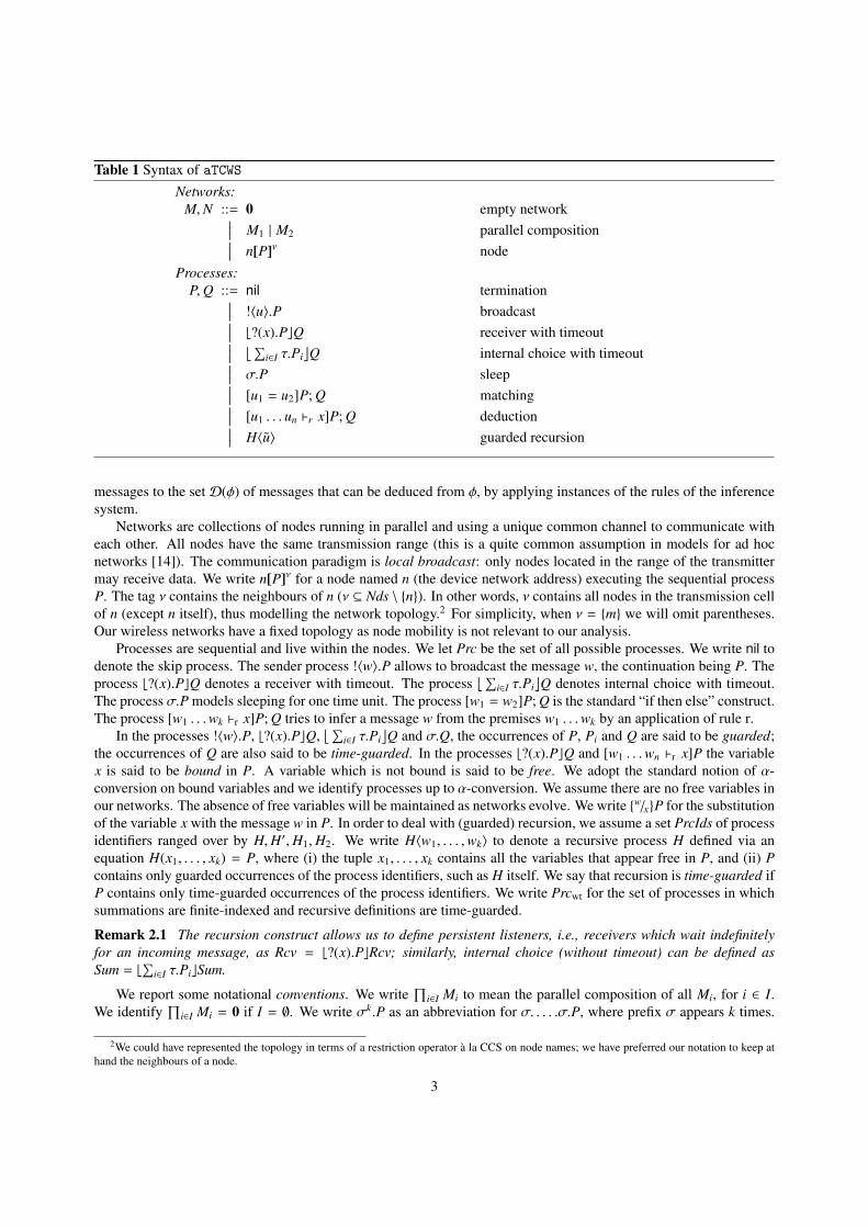
Table 1 Syntax of aTCWSNetworks:

M,N ::= 0 empty network∣∣∣ M1 | M2 parallel composition∣∣∣ n[P]ν nodeProcesses:

P,Q ::= nil termination∣∣∣ !〈u〉.P broadcast∣∣∣ b?(x).PcQ receiver with timeout∣∣∣ ⌊ ∑i∈I τ.Pi⌋Q internal choice with timeout∣∣∣ σ.P sleep∣∣∣ [u1 = u2]P; Q matching∣∣∣ [u1 . . . un `r x]P; Q deduction∣∣∣ H〈u〉 guarded recursion

messages to the setD(φ) of messages that can be deduced from φ, by applying instances of the rules of the inferencesystem.

Networks are collections of nodes running in parallel and using a unique common channel to communicate witheach other. All nodes have the same transmission range (this is a quite common assumption in models for ad hocnetworks [14]). The communication paradigm is local broadcast: only nodes located in the range of the transmittermay receive data. We write n[P]ν for a node named n (the device network address) executing the sequential processP. The tag ν contains the neighbours of n (ν ⊆ Nds \ n). In other words, ν contains all nodes in the transmission cellof n (except n itself), thus modelling the network topology.2 For simplicity, when ν = m we will omit parentheses.Our wireless networks have a fixed topology as node mobility is not relevant to our analysis.

Processes are sequential and live within the nodes. We let Prc be the set of all possible processes. We write nil todenote the skip process. The sender process !〈w〉.P allows to broadcast the message w, the continuation being P. Theprocess b?(x).PcQ denotes a receiver with timeout. The process

⌊∑i∈I τ.Pi

⌋Q denotes internal choice with timeout.

The process σ.P models sleeping for one time unit. The process [w1 = w2]P; Q is the standard “if then else” construct.The process [w1 . . .wk `r x]P; Q tries to infer a message w from the premises w1 . . .wk by an application of rule r.

In the processes !〈w〉.P, b?(x).PcQ,⌊∑

i∈I τ.Pi⌋Q and σ.Q, the occurrences of P, Pi and Q are said to be guarded;

the occurrences of Q are also said to be time-guarded. In the processes b?(x).PcQ and [w1 . . .wn `r x]P the variablex is said to be bound in P. A variable which is not bound is said to be free. We adopt the standard notion of α-conversion on bound variables and we identify processes up to α-conversion. We assume there are no free variables inour networks. The absence of free variables will be maintained as networks evolve. We write w/xP for the substitutionof the variable x with the message w in P. In order to deal with (guarded) recursion, we assume a set PrcIds of processidentifiers ranged over by H,H′,H1,H2. We write H〈w1, . . . ,wk〉 to denote a recursive process H defined via anequation H(x1, . . . , xk) = P, where (i) the tuple x1, . . . , xk contains all the variables that appear free in P, and (ii) Pcontains only guarded occurrences of the process identifiers, such as H itself. We say that recursion is time-guarded ifP contains only time-guarded occurrences of the process identifiers. We write Prcwt for the set of processes in whichsummations are finite-indexed and recursive definitions are time-guarded.

Remark 2.1 The recursion construct allows us to define persistent listeners, i.e., receivers which wait indefinitelyfor an incoming message, as Rcv = b?(x).PcRcv; similarly, internal choice (without timeout) can be defined asSum = b

∑i∈I τ.PicSum.

We report some notational conventions. We write∏

i∈I Mi to mean the parallel composition of all Mi, for i ∈ I.We identify

∏i∈I Mi = 0 if I = ∅. We write σk.P as an abbreviation for σ. . . . .σ.P, where prefix σ appears k times.

2We could have represented the topology in terms of a restriction operator a la CCS on node names; we have preferred our notation to keep athand the neighbours of a node.

3

The process [w1 = w2]P is an abbreviation for [w1 = w2]P; nil. Similarly, we will write [w1 . . .wn `r x]P to mean[w1 . . .wn `r x]P; nil.

In the sequel, we will make use of a standard notion of structural congruence to abstract over processes that differfor minor syntactic differences.

Definition 2.2 Structural congruence over networks, written ≡, is defined as the smallest equivalence relation, pre-served by parallel composition, which is a commutative monoid with respect to parallel composition and internalchoice, and for which n[H〈w〉]ν ≡ n[w/xP]ν, if H(x) = P.

Here, we provide some definitions that will be useful in the remainder of the paper. Given a network M where allnodes have distinct names, nds (M) returns the node names of M. More formally, nds (0) = ∅, nds (n[P]ν) = n andnds (M1 | M2) = nds (M1) ∪ nds (M2). For m ∈ nds (M), the function ngh(m,M) returns the set of the neighbours ofm in M. Thus, if M ≡ m[P]ν | N then ngh(m,M) = ν. We write Env (M) to mean all the nodes of the environmentreachable by the network M. Formally, Env (M) = ∪m∈nds(M)ngh(m,M) \ nds (M).

The syntax provided in Table 1 allows us to derive networks which are somehow ill-formed. The followingdefinition identifies well-formed networks. Basically, it (i) rules out networks containing two nodes with the samename; (ii) rules out self-neighbouring; (iii) imposes symmetric neighbouring relations (we recall that all nodes havethe same transmission range); (iv) imposes network connectivity to allow clock synchronisation.

Definition 2.3 (Well-formedness) M is said to be well-formed if

• M ≡ N | m1[P1]ν1 | m2[P2]ν2 implies m1 , m2;

• M ≡ N | m[P]ν implies m < ν;

• M ≡ N | m1[P1]ν1 | m2[P2]ν2 , with m1 ∈ ν2, implies m2 ∈ ν1;

• for all m, n ∈ nds (M) there are m1, . . . ,mk ∈ nds (M), such that m=m1, n=mk, mi ∈ ngh(mi+1,M), for 1 ≤ i ≤k−1.

We let Net be the set of well-formed networks.

Henceforth, we will always work with networks in Net.

2.1. Labelled transition semanticsIn Table 2, we provide a labelled transition system (LTS) for aTCWS in the SOS style of Plotkin. Intuitively,

the computation proceeds in lock-steps: between every global synchronisation all nodes proceed asynchronously byperforming actions with no duration, which represent either broadcast or input or internal actions. Transmissionproceeds even if there are no listeners: sending is a non-blocking action. Moreover, communication is lossy as somereceivers within the range of the transmitter might not receive the message. This may be due to several reasons suchas signal interferences or the presence of obstacles.

The metavariable λ ranges over the set of labels τ, σ,m!wBν,m?w denoting internal action, time passing, broad-casting and reception. Let us comment on the transition rules of Table 2. In rule (Snd) a sender m dispatches amessage w to its neighbours ν, and then continues as P. In rule (Rcv) a receiver n gets a message w coming froma neighbour node m, and then evolves into process P, where all the occurrences of the variable x are replaced withw. If no message is received in the current time slot, a timeout fires and the node n will continue with process Q,according to the rule (σ-Rcv). The rule (RcvPar) models the composition of two networks receiving the same messagefrom the same transmitter. Rule (RcvEnb) says that every node can synchronise with an external transmitter m. Noticethat a node n[b?(x).PcQ]ν might execute rule (RcvEnb) instead of rule (Rcv). This is because a potential receiver maymiss a message for several reasons (internal misbehaving, interferences, weak radio signal, etc); in this manner wemodel message loss. Rule (Bcast) models the propagation of messages on the broadcast channel. Note that this ruleloses track of the neighbours of m that are in N. Thus, in the label m!wBν the set ν always contains the neighboursof m which can receive the message w. Rule (Tau) models local computations within a node due to a nondetermin-istic internal choice. Rule (TauPar) propagates internal computations on parallel components. The remaining rulesmodel the passage of time. Rule (Sleep) models sleeping for one time slot. Rules (σ-nil) and (σ-0) are straightforward.

4

Table 2 LTS - Transmissions, internal actions and time passing

(Snd)−

m[!〈w〉.P]ν m!wBν−−−−−−−−→ m[P]ν

(Rcv)m ∈ ν

n[b?(x).PcQ]ν m?w−−−−−→ n[w/xP]ν

(RcvEnb)m < nds (M)

Mm?w−−−−−→ M

(RcvPar)M

m?w−−−−−→ M′ N

m?w−−−−−→ N′

M | Nm?w−−−−−→ M′ | N′

(Bcast)M

m!wBν−−−−−−−−→ M′ N

m?w−−−−−→ N′ µ := ν\nds (N)

M | Nm!wBµ−−−−−−−−→ M′ | N′

(Tau)h ∈ I

m[⌊∑

i∈I τ.Pi⌋Q]ν τ−−−→ m[Ph]ν

(TauPar)M

τ−−−→ M′

M | Nτ−−−→ M′ | N

(σ-nil)−

n[nil]ν σ−−−→ n[nil]ν

(Sleep)−

n[σ.P]ν σ−−−→ n[P]ν

(σ-Rcv)−

n[b?(x).PcQ]ν σ−−−→ n[Q]ν

(σ-Sum)−

m[⌊∑

i∈I τ.Pi⌋Q]ν σ−−−→ m[Q]ν

(σ-Par)M

σ−−−→ M′ N

σ−−−→ N′

M | Nσ−−−→ M′ | N′

(σ-0)−

0 σ−−−→ 0

Table 3 LTS - Matching, recursion and deduction

(Then)n[P]ν λ

−−−→ n[P′]ν

n[[w = w]P; Q]ν λ−−−→ n[P′]ν

(Else)n[Q]ν λ

−−−→ n[Q′]ν w1 , w2

n[[w1 = w2]P; Q]ν λ−−−→ n[Q′]ν

(Rec)n[w/xP]ν λ

−−−→ n[P′]ν H(x) def= P

n[H〈w〉]ν λ−−−→ n[P′]ν

(DT)n[w/xP]ν λ

−−−→ n[R]ν w1. . .wn `r w

n[[w1 . . .wn `r x]P; Q]ν λ−−−→ n[R]ν

(DF)n[Q]ν λ

−−−→ n[R]ν @ w. w1. . .wn `r w

n[[w1. . .wn `r x]P; Q]ν λ−−−→ n[R]ν

Rule (σ-Rcv) models timeout on receivers, and similarly rule (σ-Sum) describes timeout on internal activities. Rule(σ-Par) models time synchronisation between parallel components. Rules (Bcast) and (TauPar) have their symmetriccounterparts. Table 3 reports the standard rules for nodes containing matching, recursion or deduction.

Below, we report a number of basic properties of our LTS.

Proposition 2.4 Let M, M1 and M2 be well-formed networks.

1. m < nds (M) if and only if Mm?w−−−−−→ N, for some network N.

2. M1 | M2m?w−−−−−→ N if and only if there are N1 and N2 such that M1

m?w−−−−−→ N1, M2

m?w−−−−−→ N2 with N = N1 | N2.

3. If Mm!wBµ−−−−−−−−→ M′ then M ≡ m[!〈w〉.P]ν | N, for some m, ν, P and N such that m[!〈w〉.P]ν m!wBν

−−−−−−−−→ m[P]ν,N

m?w−−−−−→ N′, M′ ≡ m[P]ν | N′ and µ = ν \ nds (N).

4. If Mτ−−−→ M′ then M ≡ m[

⌊∑i∈I τ.Pi

⌋Q]ν | N, for some m, ν, Pi, Q and N such that m[

⌊∑i∈I τ.Pi

⌋Q]ν τ−−−→

m[Ph]ν, for some h ∈ I, and M′ ≡ m[Ph]ν | N.5. M1 | M2

σ−−−→ N if and only if there are N1 and N2 such that M1

σ−−−→ N1, M2

σ−−−→ N2 and N = N1 | N2.

As the topology of our networks is static it is easy to prove the following result.

5

Proposition 2.5 Let M be well-formed. If Mλ−−−→ M′ then M′ is well-formed.

Proof By induction on the derivation of the transition Mλ−−−→ M′.

2.2. Time properties

Our calculus aTCWS enjoys some desirable time properties. Here, we outline the most significant ones. Proposi-tion 2.6 formalises the deterministic nature of time passing: a network can reach at most one new state by executinga σ-action.

Proposition 2.6 (Time determinism) If M is a well-formed network with Mσ−−−→ M′ and M

σ−−−→ M′′, then M′ and

M′′ are syntactically the same.

Proof By induction on the length of the proof of Mσ−−−→ M′.

Patience guarantees that a process will wait indefinitely until it can communicate [8]. In our setting, this meansthat if no transmissions can start then it must be possible to execute a σ-action to let time pass.

Proposition 2.7 (Patience) Let M ≡∏

i∈I mi[Pi]νi be a well-formed network, such that for all i ∈ I it holds thatmi[Pi]νi . mi[!〈w〉.Qi]νi , then there is a network N such that M

σ−−−→ N.

Proof By induction on the structure of M.

The maximal progress property says that processes communicate as soon as a possibility of communicationarises [8]. In other words, the passage of time cannot block transmissions.

Proposition 2.8 (Maximal progress) Let M be a well-formed network. If M ≡ m[!〈w〉.P]ν | N then Mσ−−−→ M′ for

no network M′.

Proof By inspection on the rules that can be used to derive Mσ−−−→ M′, because sender nodes cannot perform

σ-actions.

Basically, time cannot pass unless the specification itself explicitly asks for it. This approach provides a lot ofpower to the specification, which can precisely handle the flowing of time. Such an extra expressive power leads,as a drawback, to the possibility of abuses. For instance, infinite loops of broadcast actions or internal computationsprevent time passing. The well-timedness (or finite variability) property [15] puts a limitation on the number of in-stantaneous actions that can fire between two contiguous σ-actions. Intuitively, well-timedness says that time passingnever stops: Only a finite number of instantaneous actions can fire between two subsequent σ-actions.

Definition 2.9 (Well-timedness) A network M satisfies well-timedness if there exists an upper bound k ∈ N such that

whenever Mλ1−−−→ · · ·

λh−−−→ where λ j is not directly derived by an application of (RcvEnb) and λ j , σ (for 1 ≤ j ≤ h)

then h ≤ k.

The above definition takes into account only transitions denoting an active involvement of the network, that is why wehave left out those transitions which can be derived by applying rule (RcvEnb) directly. However, as aTCWS is basicallya specification language, there is no harm in allowing specifications which do not respect well-timedness. Of course,when using our language to give a protocol implementation, then one must verify that the implementation satisfieswell-timedness: No real-world service (even attackers) can stop the passage of time.

The following proposition provides a criterion to check well-timedness. We recall that Prcwt denotes the set ofprocesses where summations are always finite-indexed and recursive definitions are always time-guarded.

Proposition 2.10 Let M =∏

i∈I mi[Pi]νi be a network. If Pi ∈ Prcwt, for all i ∈ I, then M satisfies well-timedness.

Proof First, notice that without an application of rule (RcvEnb) the network M can perform only a finite number oftransitions. Then, proceed by induction on the structure of M.

6

2.3. Behavioural semanticsBased on the LTS of Section 2.1, we define a standard notion of timed labelled similarity for aTCWS. In general,

a simulation describes how a term (in our case a network) can mimic the actions of another term. Here, we focuson weak relations, i.e., we abstract on internal actions of networks. Thus, we distinguish between the transmissionswhich may be observed and those which may not be observed by the environment. We extend the set of rules ofTable 2 with the following two rules:

(Shh)M

m!wB∅−−−−−−−−→ M′

Mτ−−−→ M′

(Obs)M

m!wBν−−−−−−−−→ M′ µ ⊆ ν µ , ∅

M!wBµ−−−−−−→ M′

Rule (Shh) models transmissions that cannot be observed because none of the potential receivers is in the environ-ment. Rule (Obs) models transmissions that can be received (and hence observed) by those nodes of the environmentcontained in ν. Notice that the name of the transmitter is removed from the label. This is motivated by the fact thatnodes may refuse to reveal their identities, e.g. for security reasons or limited sensory capabilities in perceiving theseidentities. Note also that in a derivation tree the rule (Obs) can only be applied at top-level.

In the sequel, the metavariable α will range over the following actions: τ, σ, !wBν and m?w. We adopt thestandard notation for weak transitions: the relation ==⇒ denotes the reflexive and transitive closure of

τ−−−→; the relation

α===⇒ denotes ==⇒

α−−−→==⇒; the relation α

===⇒ denotes ==⇒ if α = τ and α===⇒ otherwise.

Definition 2.11 (Similarity) A relation R over well-formed networks is a simulation if M R N and Mα−−−→ M′ imply

there is N′ such that N α===⇒ N′ and M′ R N′. We write M . N, if there is a simulation R such that M R N.

Our notion of similarity between networks is a pre-congruence, as it is preserved by parallel composition.

Theorem 2.12 Let M and N be two well-formed networks such that M . N. Then M | O . N | O for all O suchthat M | O and N | O are well-formed.

3. A tGNDC schema for wireless networks

In order to achieve a formal verification of key management protocols for WSNs, we adopt a general schema for thedefinition of timed security properties, called timed Generalized Non-Deducibility on Compositions (tGNDC) [12],a real-time generalisation of Generalized Non-Deducibility on Compositions (GNDC) [16]. The main idea is thefollowing: a system M is tGNDC ρ(M) if for every attacker A

M∣∣∣ A . ρ(M)

i.e. the composed system M | A satisfies the abstraction ρ(M).A wireless protocol involves a set of nodes which may be potentially under attack, depending on the proximity to

the attacker. This means that, in general, the attacker of a protocol M is a distinct network A of possibly colludingnodes. For the sake of compositionality, we assume that each node of the protocol is attacked by exactly one node ofA.

Definition 3.1 We say that A is a set of attacking nodes for the network M if and only if |A| = |nds (M) | andA∩ (nds (M) ∪ Env (M)) = ∅.

During the execution of the protocol an attacker may increase its initial knowledge by grasping messages sent by theparties, according to Dolev-Yao constraints.

The knowledge of a network is expressed by the set of messages that the network can manipulate. Thus, wewrite msg(P) to denote the set of the messages that appear in the process P. Formally, we follow [12] and we definemsg : Prc → 2Msg as the least set (fixed point) satisfying the rules in Table 4. A straightforward generalisation ofmsg( ) to networks is the following:

msg(0) def= ∅ ; msg(n[P]ν) def

= msg(P) ; msg(M1 | M2) def= msg(M1) ∪msg(M2) .

7

Table 4 Function msgS

msg(nil) def= ∅

msg(!〈u〉.P) def= get(u) ∪msg(P)

msg(b?(x).PcQ) def= msg(P) ∪msg(Q)

msg(⌊∑

i∈I τ.Pi⌋Q) def=⋃

i∈I msg(Pi) ∪msg(Q)

msg(σ.P) def= msg(P)

msg([u1 = u2]P; Q) def= get(u1) ∪ get(u2) ∪msg(P) ∪msg(Q)

msg([u1 . . . un `r x]P; Q) def=⋃n

i=1 get(ui) ∪msg(P) ∪msg(Q)

msg(H〈u1 . . . ur〉)def=⋃r

i=1 get(ui) ∪msg(P) if H(x) def= P

where get : Val→ 2Msg is defined as follows:

get(a) def= a (basic message)

get(x) def= ∅ (variable)

get( Fi(u1, . . . , uki ) ) def=

⋃ki

j=1 get(u j) ∪ Fi(u1, . . . , uki ) if Fi(u1 . . . uki ) ∈ Msg⋃kij=1 get(u j) otherwise.

Now, everything is in place to formally define our notion of attacker. For simplicity, in the rest of the paper, givena set of nodes N and a node n, we will write N \ n for N \ n, and N ∪ n for N ∪ n.

Definition 3.2 (Attacker) Let M be a network, with nds (M)=m1, ...,mk. LetA = a1, . . . , ak be a set of attackingnodes for M. We define the set of attackers of M atA with initial knowledge φ0 ⊆ Msg as:

Aφ0A/M

def=

k∏i=1

ai[Qi]µi : Qi ∈ Prcwt, msg(Qi) ⊆ D(φ0), µi=(A \ ai) ∪ mi

.Remark 3.3 By Proposition 2.10, the requirement Qi ∈ Prcwt in the definition of Aφ0

A/M guarantees that our attackersrespects well-timedness and hence cannot prevent the passage of time.

Sometimes, for verification reasons, we will be interested in observing part of the protocol M under examination.For this purpose, we assume that the environment contains a fresh node obs < nds (M) ∪ Env (M) ∪ A, that we callthe ‘observer’, unknown to the attacker. For convenience, the observer cannot transmit: it can only receive messages.

Definition 3.4 Let M=∏k

i=1 mi[Pi]νi . Given a set A=a1, . . . , ak of attacking nodes for M and fixed a set O ⊆nds (M) of nodes to be observed, we define:

MAO

def=

k∏i=1

mi[Pi]ν′i where ν′i

def=

(νi ∩ nds (M)) ∪ ai ∪ obs if mi ∈ O

(νi ∩ nds (M)) ∪ ai otherwise.

This definition expresses that (i) every node mi of the protocols has a dedicated attacker located at ai, (ii) networkand attacker are considered in isolation, without any external interference, (iii) only obs can observe the behaviour ofnodes in O, (iv) node obs does not interfere with the protocol as it cannot transmit, (v) the behaviour of the nodes innds (M) \ O is not observable.

We can now formalise the tGNDC family of properties as follows.

8

Definition 3.5 (tGNDC for wireless networks) Given a network M, an initial knowledge φ0, a set O ⊆ nds (M) ofnodes under observation and an abstraction ρ(M), representing a security property for M, we write M ∈ tGNDC ρ(M)

φ0,O

if and only if for some setA of attacking nodes for M and for every A ∈ Aφ0A/M it holds that

MAO

∣∣∣ A . ρ(M) .

It should be noticed that when showing that a system M is tGNDC ρ(M)φ0,O

, the universal quantification on attackersrequired by the definition makes the proof quite involved. Thus, we look for a sufficient condition which does notmake use of the universal quantification. For this purpose, we rely on a timed notion of term stability [12]. Intuitively,a network M is said to be time-dependent stable if the attacker cannot increase its knowledge in a indefinite way whenM runs in the space of a time slot. Thus, we can predict how the knowledge of the attacker evolves at each timeslot. To this purpose we need a formalisation of computation. For Λ=α1 . . . αn, we write Λ

===⇒ to denote ==⇒α1−−−−→==⇒

... ==⇒αn−−−−→==⇒. In order to count how many time slots embraces an execution trace Λ, we define #σ(Λ) to be the

number of occurrences of σ-actions in Λ.

Definition 3.6 (Time-dependent stability) A network M is said to be time-dependent stable with respect to a se-quence of knowledge φ j j≥0 if whenever MAnds(M)

∣∣∣ A Λ===⇒ M′

∣∣∣ A′, where A is a set of attacking nodes for M,

#σ(Λ) = j, A ∈ Aφ0A/M and nds (M′) = nds (M), then msg(A′) ⊆ D(φ j).

The set of messages φ j expresses the knowledge of the attacker at the end of the j-th time slot. Time-dependentstability is a crucial notion that allows us to introduce the notion of most general attacker. Intuitively, given a sequenceof knowledge φ j j≥0 and a network M, with P = nds (M), we pick a set A = a1, . . . , ak of attacking nodes for Mand we define the top attacker Tφ j

A/Pas the network which at (the beginning of) the j-th time slot is aware of the

knowledge φ j.

Definition 3.7 (Top attacker) Let M be a network, with P = nds (M)=m1, ...,mk. LetA = a1, . . . , ak be a set ofattacking nodes for M, and φ j j≥0 a sequence of knowledge. We define:

Tφ j

A/P

def=∏k

i=1 ai[Tφ j ]mi where Tφ j

def=⌊∑

w∈D(φ j) τ.!〈w〉.Tφ j

⌋Tφ j+1 .

Basically, the top attacker Tφ j

A/Pcan perform the following transitions:

• Tφ j

A/P

ai!wBmi=========⇒ Tφ j

A/P, for every i ∈ 1, . . . , k and w ∈ D(φ j)

• Tφ j

A/P

σ−−−→ Tφ j+1

A/P.

In particular, from the j-th time slot onwards, Tφ j

A/Pcan replay any message in D(φ j) to the network under attack.

Moreover, every attacking node ai can send messages to the corresponding node mi, but, unlike the attackers ofDefinition 3.2, it does not need to communicate with the other nodes in A as it already owns the full knowledge ofthe system at time j.

Remark 3.8 Notice that the top attacker ignores message causality within a single time unit. Thus, it knows allmessages in φ j already at the beginning of the time slot j. Notice also that, at each time slot, the top attacker acquiresall information that may be transmitted by the protocol at that time independently whether the information is reallytransmitted or not.

Remark 3.9 The top attacker does not satisfy well-timedness (see Definition 2.9), as the process identifiers involvedin the recursive definition are not time-guarded. However, this is not a problem as we are looking for a sufficientcondition which ensures tGNDC with respect to well-timed attackers.

A first compositional property that involves the top attacker is the following (the symbol ] denotes disjoint union).

9

Lemma 3.10 Let M = M1 | M2 be time-dependent stable with respect to a sequence of knowledge φ j j≥0. Let A1andA2 be disjoint sets of attacking nodes for M1 and M2, respectively. Let O1 ⊆ nds (M1) and O2 ⊆ nds (M2). Then

(M1 | M2)A1]A2O1]O2

∣∣∣ Tφ0A1]A2/nds(M) . M1

A1O1

∣∣∣ M2A2O2

∣∣∣ Tφ0A1/nds(M1)

∣∣∣ Tφ0A2/nds(M2) .

The following theorems say that (i) the top attacker Tφ0A/P

is strong enough for checking tGNDC, and that (ii)the notion of the most powerful attacker can be employed to reason in a compositional manner.

Theorem 3.11 (Criterion for tGNDC) Let M be time-dependent stable with respect to a sequence φ j j≥0, A be aset of attacking nodes for M and O ⊆ nds (M) = P. Then MA

O

∣∣∣ Tφ0A/P

. N implies M ∈ tGNDCNφ0,O.

The notion of the most powerful attacker is eventually employed to obtain the compositional property outlined bythe following proposition.

Theorem 3.12 (Compositionality) Let M = M1 | . . . | Mk be time-dependent stable with respect to a sequenceof knowledge φ j j≥0. Let A1, . . . ,Ak be disjoint sets of attacking nodes for M1, . . . ,Mk, respectively. Let Oi ⊆

nds (Mi) = Pi, for 1 ≤ i ≤ k. Then, (Mi)AiOi

∣∣∣ Tφ0Ai/Pi

. Ni, for 1 ≤ i ≤ k, implies M ∈ tGNDC N1 |...|Nkφ0,O1∪...∪Ok

.

Proof By Theorem 2.12 we have

(M1)A1O1

∣∣∣ . . . ∣∣∣ (Mk)AkOk

∣∣∣ Tφ0A1/nds(M1)

∣∣∣ . . . ∣∣∣ Tφ0Ak/nds(Mk) . N1

∣∣∣ . . . ∣∣∣ Nk .

By applying Lemma 3.10 and Theorem 2.12 we obtain

(M1 | . . . | Mk)A1]...]AkO1]...]Ok

∣∣∣ Tφ0A1]...]Ak/nds(M1 |...|Mk) . N1

∣∣∣ . . . ∣∣∣ Nk .

Thus, by an application of Theorem 3.11 we can derive M ∈ tGNDC N1 |...|Nkφ0,O1]...]Ok

.

3.1. Two timed security properties

As in [12], we formalise two useful timed properties for security protocols as instances of tGNDC ρφ0,O

, by suitablydefining the abstraction function ρ. We will focus on the two following timed properties:

• A timed notion of integrity, called timed integrity, which guarantees that only fresh packets are authenticated.

• A timed notion of authentication, called timed agreement, according to which if agreement is reached betweentwo parties then this must happen within a certain deadline, otherwise authentication does not hold.

More precisely, fixed a delay δ, a protocol is said to enjoy the timed integrity property if, whenever a packet pi isauthenticated during the i-th time interval, then this packet was sent at most i−δ time intervals before. For verificationreasons, when expressing time integrity in the tGNDC scheme, we will introduce in the protocol under examination aspecial message authi which is emitted only when the packet pi is authenticated.

A protocol is said to enjoy the timed agreement property if, whenever a responder n has completed a run of theprotocol, apparently with an initiator m, then m has initiated the protocol, apparently with n, at most δ time intervalsbefore, and the two agents agreed on some set of data. When expressing time agreement in the tGNDC scheme, weintroduce in the protocol under examination a special message helloi, which is emitted by the initiator at the i-th runof the protocol, and a special message endi, emitted by the responder, representing the completion of the protocollaunched at run i.

4. A security analysis of µTESLA

The µTESLA protocol was designed by Perrig et al. [17] to provide authenticated broadcast from a base station() towards all nodes of a wireless network. The protocol is based on a delayed disclosure of symmetric keys, and itrequires the network to be loosely time synchronised. The protocol computes a MAC for every packet to be broadcast,by using different keys. The transmission time is split into time intervals of ∆int time units each, and each key is tied

10

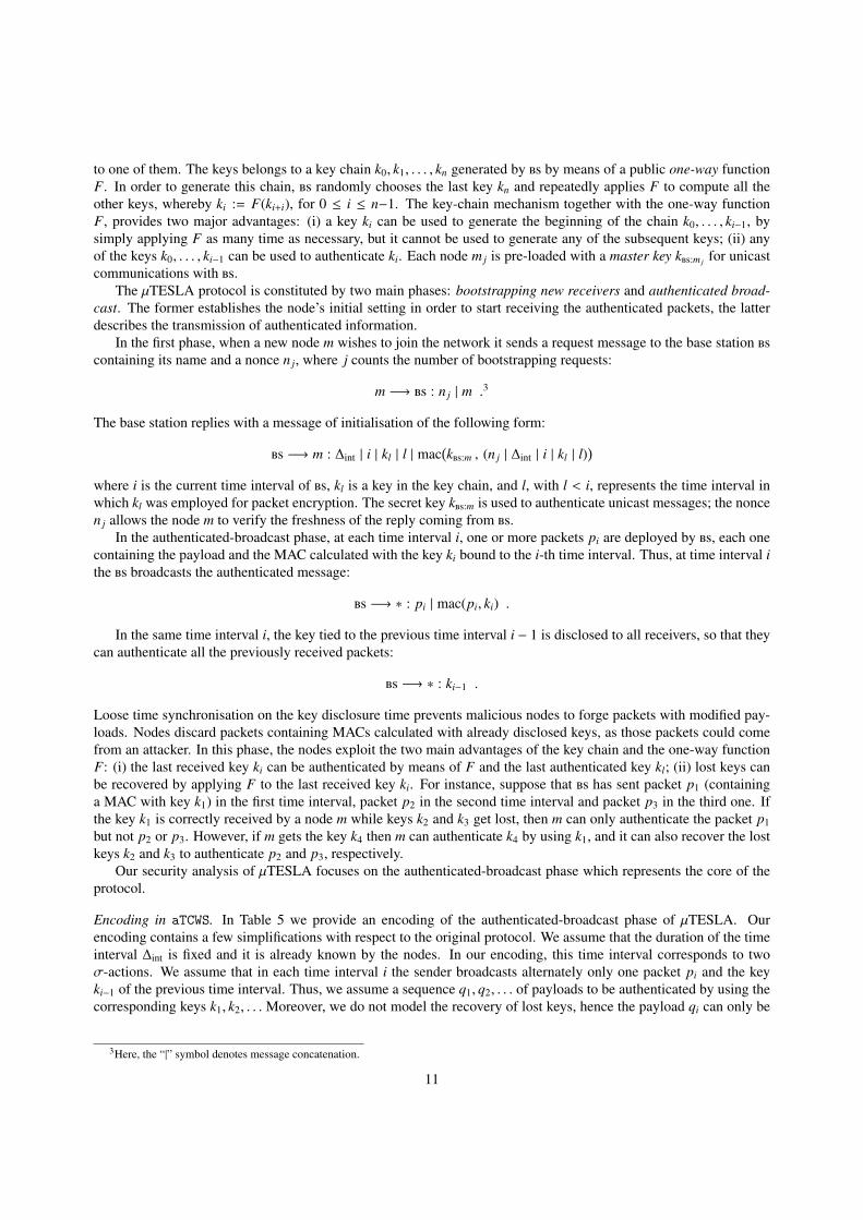
to one of them. The keys belongs to a key chain k0, k1, . . . , kn generated by by means of a public one-way functionF. In order to generate this chain, randomly chooses the last key kn and repeatedly applies F to compute all theother keys, whereby ki := F(ki+i), for 0 ≤ i ≤ n−1. The key-chain mechanism together with the one-way functionF, provides two major advantages: (i) a key ki can be used to generate the beginning of the chain k0, . . . , ki−1, bysimply applying F as many time as necessary, but it cannot be used to generate any of the subsequent keys; (ii) anyof the keys k0, . . . , ki−1 can be used to authenticate ki. Each node m j is pre-loaded with a master key k:m j for unicastcommunications with .

The µTESLA protocol is constituted by two main phases: bootstrapping new receivers and authenticated broad-cast. The former establishes the node’s initial setting in order to start receiving the authenticated packets, the latterdescribes the transmission of authenticated information.

In the first phase, when a new node m wishes to join the network it sends a request message to the base station containing its name and a nonce n j, where j counts the number of bootstrapping requests:

m −→ : n j | m .3

The base station replies with a message of initialisation of the following form:

−→ m : ∆int | i | kl | l | mac(k:m , (n j | ∆int | i | kl | l)

)where i is the current time interval of , kl is a key in the key chain, and l, with l < i, represents the time interval inwhich kl was employed for packet encryption. The secret key k:m is used to authenticate unicast messages; the noncen j allows the node m to verify the freshness of the reply coming from .

In the authenticated-broadcast phase, at each time interval i, one or more packets pi are deployed by , each onecontaining the payload and the MAC calculated with the key ki bound to the i-th time interval. Thus, at time interval ithe broadcasts the authenticated message:

−→ ∗ : pi | mac(pi, ki) .

In the same time interval i, the key tied to the previous time interval i − 1 is disclosed to all receivers, so that theycan authenticate all the previously received packets:

−→ ∗ : ki−1 .

Loose time synchronisation on the key disclosure time prevents malicious nodes to forge packets with modified pay-loads. Nodes discard packets containing MACs calculated with already disclosed keys, as those packets could comefrom an attacker. In this phase, the nodes exploit the two main advantages of the key chain and the one-way functionF: (i) the last received key ki can be authenticated by means of F and the last authenticated key kl; (ii) lost keys canbe recovered by applying F to the last received key ki. For instance, suppose that has sent packet p1 (containinga MAC with key k1) in the first time interval, packet p2 in the second time interval and packet p3 in the third one. Ifthe key k1 is correctly received by a node m while keys k2 and k3 get lost, then m can only authenticate the packet p1but not p2 or p3. However, if m gets the key k4 then m can authenticate k4 by using k1, and it can also recover the lostkeys k2 and k3 to authenticate p2 and p3, respectively.

Our security analysis of µTESLA focuses on the authenticated-broadcast phase which represents the core of theprotocol.

Encoding in aTCWS. In Table 5 we provide an encoding of the authenticated-broadcast phase of µTESLA. Ourencoding contains a few simplifications with respect to the original protocol. We assume that the duration of the timeinterval ∆int is fixed and it is already known by the nodes. In our encoding, this time interval corresponds to twoσ-actions. We assume that in each time interval i the sender broadcasts alternately only one packet pi and the keyki−1 of the previous time interval. Thus, we assume a sequence q1, q2, . . . of payloads to be authenticated by using thecorresponding keys k1, k2, . . .Moreover, we do not model the recovery of lost keys, hence the payload qi can only be

3Here, the “|” symbol denotes message concatenation.

11

Table 5 µTESLA: authenticated-broadcast phase.Sender:

S idef= [qi ki `mac ui] build MAC with payload and key

[ui qi `pair pi] build packet with mac and payload!〈pi〉.σ. broadcast packet, synchronise!〈ki−1〉.σ. broadcast previous key, synchroniseS i+1 and go to next sending state

Receiver:

R(i, l, r, kl)def= b?(p).σ.P〈i, l, p, r, kl〉c receive a pkt, synchronise, go to P

Q〈i, l, r, kl〉 if timeout go to Q

P(i, l, p, r, kl)def= b?(k).T 〈i, l, p, r, kl, k〉c receive a key k and move to T

R〈i+1, l, p, kl〉 if timeout go to next receiving state

T (i, l, p, r, kl, k) def= [F i−1−l(k) = kl] authenticate key k with F and kl

[r `fst u] extract MAC from previous pkt r[r `snd q] extract payload from r[q k `mac u′] build MAC for r with key k[u = u′] check MACs to authenticate rσ.Z〈i+1, i−1, p, r, k〉;

σ.R〈i+1, i−1, p, k〉;σ.R〈i+1, i−1, p, k〉;

σ.R〈i+1, l, p, kl〉

Z(i, l, p, r, kl)def= R〈i, l, p, kl〉 authenticated-broadcast succeeded

Q(i, l, r, kl)def= b?(k).T 〈i, l, r, r, kl, k〉c receive a key, synchronise, and

R〈i+1, l, r, kl〉 go to next receiving state

authenticated by receiving the key ki. This simplification yields a easier to read model which can be generalised tofulfil the original requirements of the protocol.

The encoding essentially defines two kind of processes: the senders S i, and the receivers R(i, l, r, kl), where i is thecurrent time interval, r is the last received packet, l is the time interval when the last key kl was authenticated. Sincewe bind one packet to one key, i also refers to the index number of packets.

The authenticated-broadcast phase of µTESLA can be represented as follows:

µTESLA def= [σ.S 1]ν

∣∣∣ m1[σ.R〈1,−1,⊥, k〉]νm1∣∣∣ . . . ∣∣∣ mh[σ.R〈1,−1,⊥, k〉]νmh

where m ∈ ν and ∈ νm, for every m ∈ m1, . . . ,mh. We use ⊥ because at the beginning there is no packet toauthenticate. We write k to denote the key transmitted by the base station and authenticated at the node’s siteduring the bootstrapping phase. Notice that k is associated to the time interval −1.

4.1. Timed integrityIn this section, we show that the authenticated-broadcast phase of µTESLA enjoys timed integrity. In particular,

we prove that receivers authenticate only packets that have been sent 2∆int time units before (that is, four σ-actionsbefore) in the correct order, even in the presence of an intruder. The crucial point is that even if an attacker acquiresthe shared keys then it is “too late” to break integrity, i.e., to authenticate packets which are more than 2∆int time unitsold.

We signal authentication of a packet r by broadcasting a special packet pair(auth, r). Thus, we replace the processR(i, l, r, kl) of Table 5 with R′(i, l, r, kl), where the process Z(i, l, p, r, kl) is replaced by

Z′(i, l, p, r, kl)def= [auth r `pair t]!〈t〉.R′〈i, l, p, kl〉 .

12

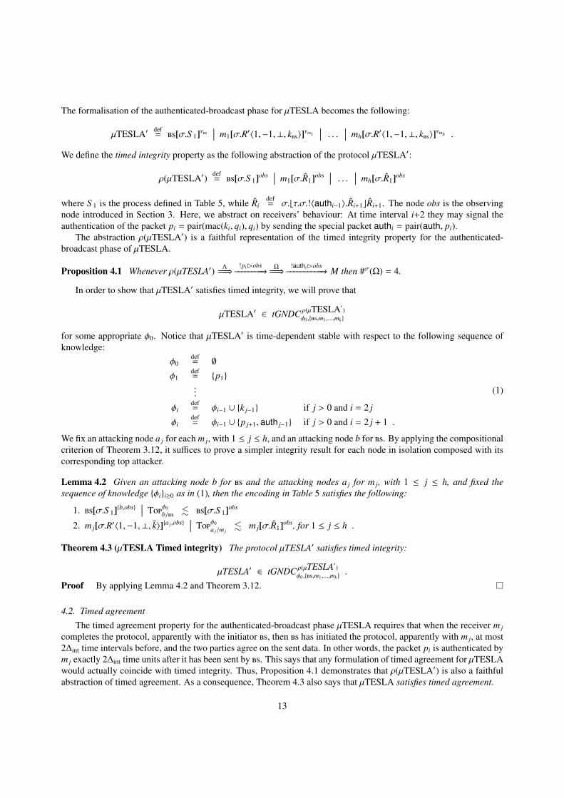
The formalisation of the authenticated-broadcast phase for µTESLA becomes the following:

µTESLA′ def= [σ.S 1]ν

∣∣∣ m1[σ.R′〈1,−1,⊥, k〉]νm1∣∣∣ . . . ∣∣∣ mh[σ.R′〈1,−1,⊥, k〉]νmh .

We define the timed integrity property as the following abstraction of the protocol µTESLA′:

ρ(µTESLA′) def= [σ.S 1]obs

∣∣∣ m1[σ.R1]obs∣∣∣ . . . ∣∣∣ mh[σ.R1]obs

where S 1 is the process defined in Table 5, while Ridef= σ.bτ.σ.!〈authi−1〉.Ri+1cRi+1. The node obs is the observing

node introduced in Section 3. Here, we abstract on receivers’ behaviour: At time interval i+2 they may signal theauthentication of the packet pi = pair(mac(ki, qi), qi) by sending the special packet authi = pair(auth, pi).

The abstraction ρ(µTESLA′) is a faithful representation of the timed integrity property for the authenticated-broadcast phase of µTESLA.

Proposition 4.1 Whenever ρ(µTESLA′) Λ===⇒

!piBobs−−−−−−−−−→

Ω===⇒

!authiBobs−−−−−−−−−−−→ M then #σ(Ω) = 4.

In order to show that µTESLA′ satisfies timed integrity, we will prove that

µTESLA′ ∈ tGNDC ρ(µTESLA′)

φ0,,m1,...,mk

for some appropriate φ0. Notice that µTESLA′ is time-dependent stable with respect to the following sequence ofknowledge:

φ0def= ∅

φ1def= p1

...

φidef= φi−1 ∪ k j−1 if j > 0 and i = 2 j

φidef= φi−1 ∪ p j+1, auth j−1 if j > 0 and i = 2 j + 1 .

(1)

We fix an attacking node a j for each m j, with 1 ≤ j ≤ h, and an attacking node b for . By applying the compositionalcriterion of Theorem 3.12, it suffices to prove a simpler integrity result for each node in isolation composed with itscorresponding top attacker.

Lemma 4.2 Given an attacking node b for and the attacking nodes a j for m j, with 1 ≤ j ≤ h, and fixed thesequence of knowledge φii≥0 as in (1), then the encoding in Table 5 satisfies the following:

1. [σ.S 1]b,obs∣∣∣ Tφ0

b/ . [σ.S 1]obs

2. m j[σ.R′〈1,−1,⊥, k〉]a j,obs∣∣∣ Tφ0

a j/m j. m j[σ.R1]obs, for 1 ≤ j ≤ h .

Theorem 4.3 (µTESLA Timed integrity) The protocol µTESLA′ satisfies timed integrity:

µTESLA′ ∈ tGNDC ρ(µTESLA′)φ0,,m1,...,mk

.

Proof By applying Lemma 4.2 and Theorem 3.12.

4.2. Timed agreement

The timed agreement property for the authenticated-broadcast phase µTESLA requires that when the receiver m j

completes the protocol, apparently with the initiator , then has initiated the protocol, apparently with m j, at most2∆int time intervals before, and the two parties agree on the sent data. In other words, the packet pi is authenticated bym j exactly 2∆int time units after it has been sent by . This says that any formulation of timed agreement for µTESLAwould actually coincide with timed integrity. Thus, Proposition 4.1 demonstrates that ρ(µTESLA′) is also a faithfulabstraction of timed agreement. As a consequence, Theorem 4.3 also says that µTESLA satisfies timed agreement.

13

5. A Security Analysis of LEAP+

The LEAP+ protocol [3] provides a keying mechanism to establish authenticated communications. The protocolis designed to establish four types of keys: an individual key, shared between a base station and a node, a single-hoppair-wise key, shared between two sensor nodes, a cluster key, shared between a node and all its neighbourhood, agroup key, shared between a base station and all sensor nodes of the network.

In this section, we focus on the single-hop pairwise key mechanism as it is underlying to all other keying methods.This mechanism is aimed at establishing a pair-wise key between a sensor node and a neighbours in ∆leap time units.In order to do that, LEAP+ exploits two peculiarities of sensor nodes: (i) the set of neighbours of a node is relativelystatic, and (ii) a sensor node that is being added to the network will discover most of its neighbours at the time of itsinitial deployment.

The single-hop pairwise shared key mechanism of LEAP+ consists of three phases.

Key pre-distribution. A network controller fixes an initial key kin and a computational efficient pseudo-random func-tion prf(). Both kin and prf() are pre-loaded in each node, before deployment. Then, each node r derives itsmaster key: kr:= prf(kin, r).

Neighbour discovery. As soon as a node m is scattered in the network area it tries to discover its neighbours bybroadcasting a hello packet that contains its identity, m, and a freshly created nonce ni, where i counts thenumber of attempts:

m −→ ∗ : m | ni .

Then each neighbour r replies with an ack message which includes its identity r, the corresponding MAC calcu-lated by using r’s master key kr, to guarantee authenticity, and the nonce ni, to guarantee freshness. Specifically:

r −→ m : r | mac(kr, (r | ni)) .

Pairwise Key Establishment. When m receives the packet q from r, it tries to authenticate it by using the last creatednonce ni and r’s master key kr = prf(kin, r). Notice that m can calculate kr as kin and prf have been pre-loadedin m, and r is contained in q. If the authentication succeeds, then both nodes proceed in calculating the pairwisekey km:r := prf(kr,m). Any other message between m and r will be authenticated by using the pairwise key km:r.If m does not get an authenticated packet from the responder in due time, it sends a new hello packet with afresh nonce.

Encoding in aTCWS. In Table 6, we provide an encoding of the single-hop pairwise shared key mechanism of LEAP+.For the sake of clarity, we assume that ∆leap consists of two time slots, i.e. it takes two σ-actions. To yield an easier toread model, we consider only two nodes and we define

LEAP+ def= m[σ.S 1]νm

∣∣∣ r[σ.R]νr

where m is the initiator, r is the responder, with m ∈ νr and r ∈ νm. Moreover, we assume that r has already computedits master key kr := prf(kin, r). This simple model does not lose in generality with respect to the multiple nodes case.

5.1. Timed Agreement

The timed agreement property for LEAP+ requires that the responder r successfully completes the protocol initi-ated by m, with the broadcasting of a hello packet, in at most ∆leap time units (i.e. two σ-actions). We will show thatLEAP+ does not satisfy the timed agreement property. Intuitively, due to the presence of the attacker, r may wronglybelieve it has established a pairwise key with m, whereas m will indefinitely send new hello packets. In some respect,this may be viewed as a kind of denial-of-service attack.

For our analysis, in order to make observable the completion of the protocol, we define LEAP′+ by replacing inLEAP+ the process R of Table 6 with the process R′ defined as the same as R except for process R6 which is replacedby

R6′ def= σ.[end n `pair e]!〈e〉.nil .

14

Table 6 LEAP+ specificationSender at node m:

S idef= [ni−1 m `pr f ni] build a random nonce ni

[m ni `pair t] build a pair t with m and the nonce ni

[hello t `pair p] build hello packet using the pair t!〈p〉.σ.P broadcast hello, synchronise and move to P

P def= b?(q).P1cS i+1 wait for response from neighbours

P1 def= [q ` f st r]P2;σ.S i+1 extract node name r from packet q,

P2 def= [q `snd h] extract MAC h from packet q

[r ni `pair t′] build a pair t′ with r and current nonce ni

[kin r `pr f kr] calculate r’s master key kr

[kr t′ `mac h′] calculate MAC h′ with kr and t′

[h′ = h]P3;σ.S i+1 if it matches with the received one go to P3,otherwise go to next time unit and restart

P3 def= [kr m `pr f km:r]P4 calculate the pairwise key km:r

P4 def= σ.nil synchronise and conclude key establishment

Receiver at node r:

R def= b?(p).R1cσ.R wait for incoming hello packets

R1 def= [p ` f st p1]R2;σ.σ.R extract the first component

R2 def= [p `snd p2] extract the second component

[p1 = hello]R3;σ.σ.R check if p is a hello packet

R3 def= [p2 ` f st m]R4;σ.σ.R extract the sender name m

R4 def= [p2 `snd n] extract the nonce n

[r n `pair t] build a pair t with n and r[kr t `mac h] calculate MAC h on t with r’s master key kr

[r h `pair q] build packet q with node name r and MAC hσ.!〈q〉.R5 synchronise, broadcast q and go to R5

R5 def= [kr m `pr f km:r]R6 calculate pairwise key km:r

R6 def= σ.nil synchronise and conclude key establishment

We use the following abbreviations: helloidef= pair(hello, pair(m, ni)) and endi

def= pair(end, ni).

The timed agreement property of LEAP+ is defined by the following abstraction:

ρagr(LEAP′+) def= m[σ.S 1]obs | r[σ.R1]obs

where S idef= !〈helloi〉.σbτ.σ.nilcS i+1 and Ri

def= bτ.σ!〈qi〉.σ.!〈endi〉.nilcσ.Ri+1, with qi = pair(r,mac(kr, pair(r, ni))),

as defined in Table 6.The following statement says that the abstraction ρagr(LEAP′+) expresses correctly the timed agreement property

for LEAP+.

Proposition 5.1 Whenever ρagr(LEAP′+) Λ===⇒

!helloiBobs−−−−−−−−−−−→

Ω===⇒

!endiBobs−−−−−−−−−−−→ then #σ(Ω) = 2.

Now, in order to prove timed agreement for LEAP+ we should show that

LEAP′+ ∈ tGNDC ρagr(LEAP′+)φ0,m,r

15

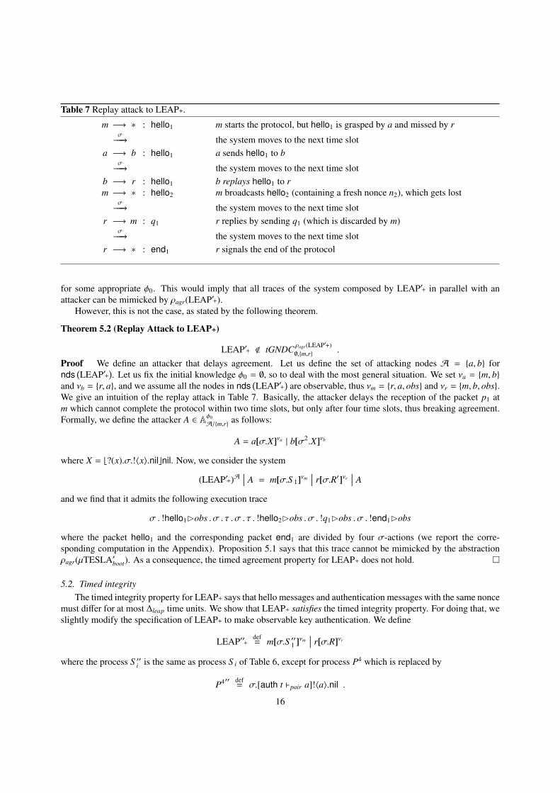
Table 7 Replay attack to LEAP+.

m −→ ∗ : hello1 m starts the protocol, but hello1 is grasped by a and missed by rσ−−−→ the system moves to the next time slot

a −→ b : hello1 a sends hello1 to bσ−−−→ the system moves to the next time slot

b −→ r : hello1 b replays hello1 to rm −→ ∗ : hello2 m broadcasts hello2 (containing a fresh nonce n2), which gets lost

σ−−−→ the system moves to the next time slot

r −→ m : q1 r replies by sending q1 (which is discarded by m)σ−−−→ the system moves to the next time slot

r −→ ∗ : end1 r signals the end of the protocol

for some appropriate φ0. This would imply that all traces of the system composed by LEAP′+ in parallel with anattacker can be mimicked by ρagr(LEAP′+).

However, this is not the case, as stated by the following theorem.

Theorem 5.2 (Replay Attack to LEAP+)

LEAP′+ < tGNDC ρagr(LEAP′+)∅,m,r .

Proof We define an attacker that delays agreement. Let us define the set of attacking nodes A = a, b fornds(LEAP′+

). Let us fix the initial knowledge φ0 = ∅, so to deal with the most general situation. We set νa = m, b

and νb = r, a, and we assume all the nodes in nds(LEAP′+

)are observable, thus νm = r, a, obs and νr = m, b, obs.

We give an intuition of the replay attack in Table 7. Basically, the attacker delays the reception of the packet p1 atm which cannot complete the protocol within two time slots, but only after four time slots, thus breaking agreement.Formally, we define the attacker A ∈ Aφ0

A/m,r as follows:

A = a[σ.X]νa | b[σ2.X]νb

where X = b?(x).σ.!〈x〉.nilcnil. Now, we consider the system

(LEAP′+)A∣∣∣ A = m[σ.S 1]νm

∣∣∣ r[σ.R′]νr∣∣∣ A

and we find that it admits the following execution trace

σ . !hello1Bobs . σ . τ . σ . τ . !hello2Bobs . σ . !q1Bobs . σ . !end1Bobs

where the packet hello1 and the corresponding packet end1 are divided by four σ-actions (we report the corre-sponding computation in the Appendix). Proposition 5.1 says that this trace cannot be mimicked by the abstractionρagr(µTESLA′boot). As a consequence, the timed agreement property for LEAP+ does not hold.

5.2. Timed integrityThe timed integrity property for LEAP+ says that hello messages and authentication messages with the same nonce

must differ for at most ∆leap time units. We show that LEAP+ satisfies the timed integrity property. For doing that, weslightly modify the specification of LEAP+ to make observable key authentication. We define

LEAP′′+ def= m[σ.S ′′1 ]νm

∣∣∣ r[σ.R]νr

where the process S ′′i is the same as process S i of Table 6, except for process P4 which is replaced by

P4′′ def= σ.[auth t `pair a]!〈a〉.nil .

16

For simplicity, we use the following abbreviation: authi = pair(auth, pair(m, ni)).In order to formally represent the timed integrity property, we define the following abstraction of the protocol:

ρint(LEAP′′+) def= m[σ.S 1]obs

∣∣∣ r[Tick]∅

where S idef= !〈helloi〉.σ.

⌊τ.σ.!〈authi〉.nil

⌋S i+1 and Tick def

= σ.Tick .By construction, ρint(LEAP′′+) is a faithful representation of timed integrity for LEAP+ (we recall that in our

encoding ∆leap corresponds to two σ-actions).

Proposition 5.3 Whenever ρint(LEAP′′+) Λ===⇒

!helloiBobs−−−−−−−−−−−→

Ω===⇒

!authiBobs−−−−−−−−−−→ M then #σ(Ω) = 2.

Now, we notice that LEAP′′+ is time-dependent stable with respect to the sequence of knowledge φii≥0, definedas follows:

φ0def= ∅

φ1def= hello1

...

φidef= φi−1 ∪ mac(kr, pair(r, n j)) if j > 0 and i = 2 j

φidef= φi−1 ∪ hello j+1, auth j if j > 0 and i = 2 j + 1 .

(2)

Now, we pick two attacking nodes a and b, for m and r, respectively, and we focus on the observation of node m asit signals both the beginning and the end of the authentication protocol. Again, by applying Theorem 3.12 it sufficesto prove a simpler result for each node in isolation composed with its corresponding top attacker.

Lemma 5.4 Given two attacking nodes a and b, for m and r respectively, and fixed the sequence of knowledge φii≥0as in (2), then

1. m[σ.S ′′1 ]a,obs∣∣∣ Tφ0

a/m . m[σ.S 1]obs

2. r[σ.R]b∣∣∣ Tφ0

b/r . r[Tick]∅ .

Theorem 5.5 (LEAP+ Timed integrity) LEAP′′+ satisfies the timed integrity property:

LEAP′′+ ∈ tGNDC ρint(LEAP′′+)φ0,m

.

Proof By applying Lemma 5.4 and Theorem 3.12.

6. A security analysis of LiSP

In order to achieve a good trade-off between resource limitations and network security, Park et al. [2] have pro-posed a Lightweight Security Protocol (LiSP) for WSNs. LiSP provides (i) an efficient key renewal mechanism whichavoids key retransmission, (ii) authentication for each key-disclosure, and (iii) the possibility of both recovering anddetecting lost keys.

A LiSP network consists of a Key Server () and a set of sensor nodes m1, . . . ,mk. The protocol assumes aone way function F, pre-loaded in every node of the system, and employs two different key families: (i) a set oftemporal keys k0, . . . , kn, computed by by means of F, and used by all nodes to encrypt/decrypt data packets; (ii) aset of master keys k:m j , one for each node m j, for unicast communications between m j and . As in µTESLA, thetransmission time is split into time intervals, each of them is ∆refresh time units long. Thus, each temporal key is tiedto a time interval and renewed every ∆refresh time units. At a time interval i, the temporal key ki is shared by all sensornodes and it is used for data encryption. Key renewal relies on loose node time synchronisation among nodes. Eachnode stores a subset of temporal keys in a buffer of a fixed size, say s with s << n.

The LiSP protocol consists of the following phases.

17

Initial Setup. At the beginning, randomly chooses a key kn and computes a sequence of temporal keys k0, . . . , kn, byusing the function F, as ki := F(ki+1). Then, waits for reconfiguration requests from nodes. More precisely,when receives a reconfiguration request from a node m j, at time interval i, it unicasts the packet InitKey:

−→ m j : enc(k:m j , (s | ks+i | ∆refresh)) | hash(s | ks+i | ∆refresh) .

The operator enc(k, p) represents the encryption of p by using the key of k, while hash(p) generates a messagedigest for p by means of a cryptographic hash function used to check the integrity of the packet p. Whenm j receives the InitKey packet, it computes the sequence of keys ks+i−1, ks+i−2, . . . , ki by several applicationsof the function F to ks+i. Then, it activates ki for data encryption and it stores the remaining keys in its localbuffer; finally it sets up a ReKeyingTimer to expires after ∆refresh/2 time units (this value applies only for thefirst rekeying).

Re-Keying. At each time interval i, with i ≤ n, employs the active encryption key ki to encode the key ks+i. Theresulting packet is broadcast as an UpdateKey packet:

−→ ∗ : enc(ki, ks+i) .

When a node receives an UpdateKey packet, it tries to authenticate the key received in the packet; if the nodesucceeds in the authentication then it recovers all keys that have been possibly lost and updates its key buffer.When the time interval i elapses, every node discards ki, activates the key ki+1 for data encryption, and setsup the ReKeyingTimer to expire after ∆refresh time units for future key switching (after the first time, switchinghappens every ∆refresh time units).

Authentication and Recovery of Lost Keys. The one-way function F is used to authenticate and recover lost keys. If lis the number of stored keys in a buffer of size s, with l ≤ s, then s− l represents the number of keys which havebeen lost by the node. When a sensor node receives an UpdateKey packet carrying a new key k, it calculatesF s−l(k) by applying s − l times the function F. If the result matches with the last received temporal key, thenthe node stores k in its buffer and recovers all lost keys.

Reconfiguration. When a node m j joins the network or misses more than s temporal keys, then its buffer is empty.Thus, it sends a RequestKey packet in order to request the current configuration:

m j −→ : RequestKey | m j .

Upon reception, node performs authentication of m j and, if successful, it sends the current configuration viaan InitKey packet.

Encoding. In Table 8, we provide a specification in aTCWS of the entire LiSP protocol. We introduce some slightsimplifications with respect to the original protocol. We assume that (i) the temporal keys k0, . . . , kn have already beencomputed by , (ii) both the buffer size s and the refresh interval ∆refresh are known by each node. Thus, the InitKeypacket can be simplified as follows:

−→ m j : enc(k:m j , ks+i) | hash(ks+i) .

Moreover, we assume that every σ-action models the passage of ∆refresh/2 time units. Therefore, every two σ-actionsthe key server broadcasts the new temporal key encrypted with the key tied to that specific interval. Finally, we do notmodel data encryption.

When giving our encoding in aTCWS we will require some new deduction rules to model an hash function andencryption/decryption of messages:

(hash)w

hash(w)(enc)

w1 w2

enc(w1,w2)(dec)

w1 w2

dec(w1,w2).

The protocol executed by the key server is expressed by the following two threads: a key distributor Di and alistener Li waiting for reconfiguration requests from the sensor nodes, with i being the current time interval. Every

18

Table 8 The LiSP protocol

Key Server:

D0def= σ.D1 synchronise and move to D1

Didef= [ki ks+i `enc ti] for i ≥ 1, encrypt ks+i with ki

[UpdateKey ti `pair ui] build the UpdateKey packet ui

!〈ui〉.σ.σ.Di+1 broadcast ri, and move to Di+1

Lidef= b?(r).Ii+1cσ.Li+1 wait for request packets

Iidef= [r ` f st r1]I1

i ;σ.σ.Li extract first component

I1i

def= [r1 = RequestKey]I2

i ;σ.σ.Li check if r1 is a RequestKey

I2i

def= [r `snd m] extract node name

[k:m ks+i `enc wi] encrypt ks+i with k:m[ks+i `hash hi] calculate hash code for ks+i

[wi hi `pair ri] build a pair ri,[InitKey ri `pair qi] build a InitKey packet qi,σ.!〈qi〉.σ.Li broadcast qi, move to Li

Receiver at node m:

Z def= [RequestKey m `pair r] send a RequestKey packet

!〈r〉.σ.b?(q).T cZ wait for a reconfig. packet

T def= [q ` f st q′]T 1;σ.Z extract fst component of q

T 1 def= [q′ = InitKey]T 2;σ.Z check if q is a InitKey packet

T 2 def= [q `snd q′′] extract snd component of q

[q′′ ` f st w]T 3;σ.Z extract fst component of q′′

T 3 def= [q′′ `snd h] extract snd component of q′′

[k:m w `dec k]T 3;σ.Z extract the key

T 4 def= [k `hash h′][h = h′]T 5;σ.Z verify hash codes

T 5 def= σ.σ.R〈F s−1(k), k, s−1〉 synchronise and move to R

R(k, k, l)def= b?(u).EcF wait for incoming packets

E def= [u ` f st u′]E1;σ.F extract fst component of u

E1 def= [u′ = UpdateKey]E2;σ.F check UpdateKey packet

E2 def= [u `snd u′′] extract snd component of u

[k u′′ `dec k]E3;σ.F decrypt u′′ by using kE3 def

= [F s−l(k) = k]E4;σ.F authenticate k

E4 def= σ.σ.R〈F s−1(k), k, s−1〉 synchronise and move to R

F def= [l = 0]Z;σ.R〈F l−1(k), k, l−1〉 check if buffer key is empty

∆refresh time units (that is, every two σ-actions) Di broadcasts the new temporal key ks+i encrypted with the key ki ofthe current time interval i. The process Li replies to reconfiguration requests by sending an initialisation packet.

At the beginning of the protocol, a sensor node runs the process Z, which broadcasts a request packet to , waitsfor a reconfiguration packet q, and then checks authenticity by verifying the hash code. If the verification is successfulthen the node starts the broadcasting new keys phase. This phase is formalised by the process R(k, k, l), where k isthe current temporal key, k is the last authenticated temporal key, and the integer l counts the number of keys that areactually stored in the buffer.

To simplify the exposition, we formalise the key server as a pair of nodes: a key disposer , which executes Di,

19

and a listener , which executes Li. Thus, the LiSP protocol, in its initial configuration, can be represented as:

LiSP def=∏j∈J

m j[σ.Z]νm j | [σ.L0]ν | [σ.D0]ν

where for each node m j, with j ∈ J, m j ∈ ν ∩ ν and , ⊆ νm j .

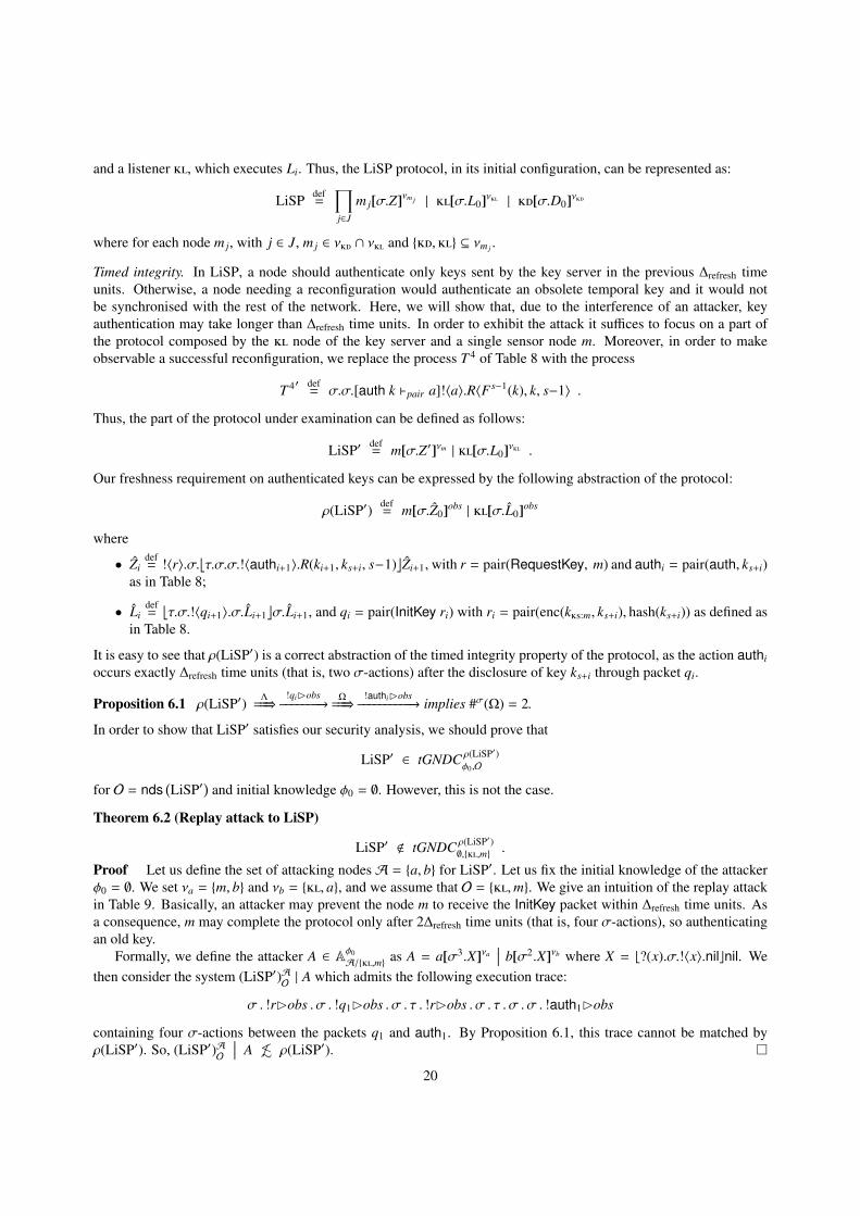
Timed integrity. In LiSP, a node should authenticate only keys sent by the key server in the previous ∆refresh timeunits. Otherwise, a node needing a reconfiguration would authenticate an obsolete temporal key and it would notbe synchronised with the rest of the network. Here, we will show that, due to the interference of an attacker, keyauthentication may take longer than ∆refresh time units. In order to exhibit the attack it suffices to focus on a part ofthe protocol composed by the node of the key server and a single sensor node m. Moreover, in order to makeobservable a successful reconfiguration, we replace the process T 4 of Table 8 with the process

T 4′ def= σ.σ.[auth k `pair a]!〈a〉.R〈F s−1(k), k, s−1〉 .

Thus, the part of the protocol under examination can be defined as follows:

LiSP′ def= m[σ.Z′]νm | [σ.L0]ν .

Our freshness requirement on authenticated keys can be expressed by the following abstraction of the protocol:

ρ(LiSP′) def= m[σ.Z0]obs | [σ.L0]obs

where

• Zidef= !〈r〉.σ.

⌊τ.σ.σ.!〈authi+1〉.R(ki+1, ks+i, s−1)

⌋Zi+1, with r = pair(RequestKey, m) and authi = pair(auth, ks+i)

as in Table 8;

• Lidef=⌊τ.σ.!〈qi+1〉.σ.Li+1

⌋σ.Li+1, and qi = pair(InitKey ri) with ri = pair(enc(k:m, ks+i), hash(ks+i)) as defined as

in Table 8.

It is easy to see that ρ(LiSP′) is a correct abstraction of the timed integrity property of the protocol, as the action authi

occurs exactly ∆refresh time units (that is, two σ-actions) after the disclosure of key ks+i through packet qi.

Proposition 6.1 ρ(LiSP′) Λ===⇒

!qiBobs−−−−−−−−→

Ω===⇒

!authiBobs−−−−−−−−−−−→ implies #σ(Ω) = 2.

In order to show that LiSP′ satisfies our security analysis, we should prove that

LiSP′ ∈ tGNDC ρ(LiSP′)φ0,O

for O = nds(LiSP′

)and initial knowledge φ0 = ∅. However, this is not the case.

Theorem 6.2 (Replay attack to LiSP)

LiSP′ < tGNDC ρ(LiSP′)∅,,m .

Proof Let us define the set of attacking nodesA = a, b for LiSP′. Let us fix the initial knowledge of the attackerφ0 = ∅. We set νa = m, b and νb = , a, and we assume that O = ,m. We give an intuition of the replay attackin Table 9. Basically, an attacker may prevent the node m to receive the InitKey packet within ∆refresh time units. Asa consequence, m may complete the protocol only after 2∆refresh time units (that is, four σ-actions), so authenticatingan old key.

Formally, we define the attacker A ∈ Aφ0A/,m as A = a[σ3.X]νa

∣∣∣ b[σ2.X]νb where X = b?(x).σ.!〈x〉.nilcnil. Wethen consider the system (LiSP′)A

O| A which admits the following execution trace:

σ . !rBobs . σ . !q1Bobs . σ . τ . !rBobs . σ . τ . σ . σ . !auth1Bobs

containing four σ-actions between the packets q1 and auth1. By Proposition 6.1, this trace cannot be matched byρ(LiSP′). So, (LiSP′)A

O

∣∣∣ A 6. ρ(LiSP′).

20

Table 9 Replay attack to LiSP

m −→ : r m sends a RequestKey and correctly receives the packetσ−−−→ the system moves to the next time slot

−→ m : q1 replies with an InitKey which is lost by m and grasped by bσ−−−→ the system moves to the next time slot

b −→ a : q1 b sends q1 to am −→ : r m sends a new RequestKey which gets lost

σ−−−→ the system moves to the next time slot

a → m : q1 a replays q1 to mσ−−−→

σ−−−→ after ∆refresh time units

m −→ ∗ : auth1 m authenticates q1 and signals the end of the protocol

6.1. Timed agreementThe timed agreement property for LiSP requires that when a sensor node m completes the protocol, apparently

with the initiator , then has initiated the protocol, apparently with m, at most ∆refresh time units before, and the twoparties agree on the transmitted data. In other words: the packet qi must be received and authenticated by m exactly∆refresh time units after it has been sent by . This suggests that any formulation of timed agreement for LiSP wouldactually coincide with timed integrity. Thus, Proposition 6.1 demonstrates that ρ(LiSP′) is also a faithful abstractionof timed agreement. As a consequence, Theorem 6.2 also says that LiSP does not satisfies timed agreement.

7. Conclusions, Related and Future Work

We have proposed a timed broadcasting calculus, called aTCWS, to formalise and verify real-world key manage-ment protocols for WSNs. Our calculus comes with a well-defined operational semantics and a simulation-basedbehavioural semantics. Then, we have revised Gorrieri and Martinelli’s tGNDC framework [12] in such a way that itcan be applied to WSNs. We have used tGNDC to express two timed properties of wireless security protocols: timedintegrity and timed agreement. A nice aspect of expressing a security property as a tGNDC-property is that when itdoes not hold then it is possible to exhibit an attack which invalidate the property. In order to prove tGNDC-propertiesin an effective manner, we have provided a compositional proof technique based on the notion of the most powerfulattacker. Notice that, as pointed out in Remarks 3.8 and 3.9, the top attacker used in our proof technique is slightlymore powerful than any process in aTCWS. As a consequence, our proof technique for tGNDC is sound but not com-plete. Nevertheless, when a protocol can be attacked by the top attacker there are good chances that the same attackcan be perpetrated by a real attacker.

We have provided formal specifications in aTCWS of three well-known key management protocols for WSNs:µTESLA [1], LEAP+ [3] and LiSP [2]. Our specifications meet the requirements of Proposition 2.10, thus they allsatisfy well-timedness. Then, we have formally proved that the single-hop pairwise shared key mechanism of LEAP+enjoys timed integrity, and that the authenticated-broadcast phase of µTESLA enjoys both timed integrity and timedagreement. We have provided two different replay attacks to show that the single-hop pairwise shared key mechanismof LEAP+ do not enjoy timed agreement, and that LiSP satisfies neither timed integrity nor timed agreement. Thekind of attack occurring in LiSP cannot be repeated in LEAP+ or µTESLA as these two protocols assume the presenceof nonces which guarantee message freshness. We could use the same precaution in LiSP, by adding a nonce in allRequestKey and InitKey packets [18]. However, as seen for LEAP+ the addition of nonces in LiSP would fix timedintegrity but not timed agreement.

The present work is the continuation and generalisation of [19], where a slight variant of the calculus was intro-duced, and an early security analysis for the authenticated-broadcast phase of µTESLA and the single-hop pairwiseshared key mechanism of LEAP+ was performed. In [18] the calculus aTCWS has been used to analyse the LiSP proto-col. The design of our calculus is strongly inspired by tCryptoSPA [12], a timed “cryptographic” variant of Milner’sCCS [20], where node distribution, local broadcast communication and message loss are codified in terms of point-to-point transmission and a discrete notion of time. As a consequence, specifications and security analyses of wireless

21

network protocols in tCryptoSPA are much more complicated than ours. The tGNDC schema for tCryptoSPA, hasalready been used by Gorrieri et al. [13] to study a number security protocols, for both wired and wireless networks.In particular, they studied the authenticated-broadcast phase of µTESLA, proving timed integrity. The formalisationfor µTESLA we have proposed here is much less involved than the one of [13] thanks to the specific features of ourcalculus for broadcast communications.

Several process calculi for wireless systems have been recently proposed. Mezzetti and Sangiorgi [21] haveintroduced a calculus to describe interferences in wireless systems. Nanz and Hankin [22] have proposed a calculus formobile ad hoc networks for specification and security analysis of communication protocols. They provide a decisionprocedure to check security against fixed intruders known in advance. Merro [23] has proposed a behavioural theoryfor mobile ad hoc networks. Godskesen [24] has proposed a calculus for mobile ad hoc networks with a formalisationof an attack on the cryptographic routing protocol ARAN. Singh et al. [25] have proposed theω-calculus for modellingthe AODV routing protocol. Ghassemi et al. [26, 27] have proposed a process algebra, provided with model checkingand equational reasoning, which models topology changes implicitly in the semantics. Merro and Sibilio [28] haveproposed a timed calculus for wireless systems focusing on the notion of communication collision. Godskesen andNanz [29] have proposed a simple timed calculus for wireless systems to express a wide range of mobility models.Gallina and Rossi [30] have proposed a calculus for the analysis of energy-aware communications in mobile adhoc networks. Song and Godskesen [31] have proposed the first probabilistic un-timed calculus for mobile wirelesssystems in which connection probabilities may change due to node mobility. Kouzapas and Philippou [32] haveproposed a process calculus for dynamic networks which contains features for broadcasting at multiple transmissionranges and for viewing networks at different levels of abstraction.

Recently, Arnaud et al. [33] have proposed a calculus for modelling and reasoning about security protocols, in-cluding secure routing protocols, for a bounded number of sessions. They provide two NPTIME decision proceduresfor analysing routing protocols for any network topology, and apply their framework to analyse the protocol SRP [34]applied to DSR [35].

The AVISPA model checker [36] has been used in [37] for an analysis of TinySec [38], LEAP [39], and TinyPK [40],three wireless sensor network security protocols, and in [41] for an analysis of the Sensor Network Encryption Proto-col SNEP [1]. In particular, in [37] the authors considered the communication between immediate neighbour nodeswhich use the pairwise shared key already established by LEAP. In this case AVISPA found a man-in-the-middleattack where the intruder may play at the same time the role of two nodes in order to obtain real information from oneof them, thus loosing confidentiality.

It is our intention to apply our framework to study the correctness of a wide range of wireless network securityprotocols, as for instance, MiniSec [42], and evolutions of LEAP+, such as R-LEAP+ [43] and LEAP++ [44].

Acknowledgements. The referees have provided several useful comments.

References

[1] A. Perrig, R. Szewczyk, J. D. Tygar, V. Wen, D. Culler, SPINS: Security Protocols for Sensor Networks, Wireless Networks 8 (5) (2002)521–534.

[2] T. Park, K. G. Shin, LiSP: A Lightweight Security Protocol for Wireless Sensor Networks, ACM Transactions on Embedded ComputingSystems (TECS) 3 (3) (2004) 634–660.

[3] S. Zhu, S. Setia, S. Jajodia, LEAP+: Efficient Security Mechanisms For Large-Scale Distributed Sensor Networks, ACM Transactions onSensor Networks 2 (4) (2006) 500–528.

[4] S. Basagni, K. Herrin, D. Bruschi, E. Rosti, Secure Pebblenets, in: ACM International Symposium on Mobile Ad Hoc Networking andComputing (MobiHoc), 156–163, 2001.

[5] R. J. Anderson, H. Chan, A. Perrig, Key Infection: Smart Trust for Smart Dust, in: IEEE International Conference on Network Protocols(ICNP), 206–215, 2004.

[6] W. Diffiel, M. E. Hellman, New Directions in Cryptography, IEEE Transactions on Information Theory 22 (6) (1976) 644–654.[7] R. L. Rivest, A. Shamir, L. M. Adleman, A Method for Obtaining Digital Signatures and Public-Key Cryptosystems, Communications of the

ACM 21 (2) (1978) 120–126.[8] M. Hennessy, T. Regan, A Process Algebra for Timed Systems, Information and Computation 117 (2) (1995) 221–239.[9] B. Sundararaman, U. Buy, A. D. Kshemkalyani, Clock Synchronization for Wireless Sensor Networks: a Survey, Ad Hoc Networks 3 (3)

(2005) 281–323.[10] T. Nipkow, L. C. Paulson, M. Wenzel, Isabelle/HOL - A Proof Assistant for Higher-Order Logic, vol. 2283 of Lecture Notes in Computer

Science, Springer, 2002.

22

[11] Y. Bertot, A Short Presentation of Coq, in: International Conference on Theorem Proving in Higher Order Logics (TPHOLs 2007), vol. 5170of LNCS, 12–16, 2008.

[12] R. Gorrieri, F. Martinelli, A Simple Framework for Real-Time Cryptographic Protocol Analysis with Compositional Proof Rules, Science ofComputer Programming 50 (1-3) (2004) 23–49.

[13] R. Gorrieri, F. Martinelli, M. Petrocchi, Formal Models and Analysis of Secure Multicast in Wired and Wireless Networks, Journal ofAutomated Reasoning 41 (3-4) (2008) 325–364.

[14] S. Misra, I. Woungag, Guide to Wireless Ad Hoc Networks, Computer Communications and Networks, Springer London, ISBN 978-1-84800-327-9, 2009.

[15] X. Nicollin, J. Sifakis, An Overview and Synthesis on Timed Process Algebras, in: International Workshop on Computer Aided Verification(CAV), vol. 575 of Lecture Notes in Computer Science, Springer, 376–398, 1991.

[16] R. Focardi, F. Martinelli, A Uniform Approach for the Definition of Security Properties, in: World Congress on Formal Methods (FM), vol.1708 of Lecture Notes in Computer Science, Springer, 794–813, 1999.

[17] A. Perrig, R. Szewczyk, V. Wen, D. E. Culler, J. D. Tygar, SPINS: Security Protocols for Sensor Netowrks, in: International Conference onMobile Computing and Networking (MOBICOM), 189–199, 2001.

[18] D. Macedonio, M. Merro, A Semantics Analysis of Wireless Network Security Protocols, in: NASA Formal Methods Symposium (NFM),vol. 7226 of Lecture Notes in Computer Science, Springer, Heidelberg, 403–417, 2012.

[19] F. Ballardin, M. Merro, A Calculus for the Analysis of Wireless Network Security Protocols, in: Formal Aspects in Security and Trust(FAST), vol. 6561 of Lecture Notes in Computer Science, Springer, 206–222, 2010.

[20] R. Milner, Communication and Concurrency, Prentice Hall, 1989.[21] I. Lanese, D. Sangiorgi, An Operational Semantics for a Calculus for Wireless Systems, Theoretical Computer Science 411 (2010) 1928–

1948.[22] S. Nanz, C. Hankin, A Framework for Security Analysis of Mobile Wireless Networks, Theoretical Computer Science 367 (1-2) (2006)

203–227.[23] M. Merro, An Observational Theory for Mobile Ad Hoc Networks (full paper), Information and Computation 207 (2) (2009) 194–208.[24] J. Godskesen, A Calculus for Mobile Ad Hoc Networks, in: Coordination Models and Languages (COORDINATION), vol. 4467 of Lecture

Notes in Computer Science, Springer, 132–150, 2007.[25] A. Singh, C. R. Ramakrishnan, S. A. Smolka, A Process Calculus for Mobile Ad Hoc Networks, in: Coordination Models and Languages

(COORDINATION), vol. 5052 of Lecture Notes in Computer Science, Springer, 296–314, 2008.[26] F. Ghassemi, W. Fokkink, A. Movaghar, Equational Reasoning on Mobile Ad Hoc Networks, Fundamenta Informaticae 105 (4) (2010)

375–415.[27] F. Ghassemi, W. Fokkink, A. Movaghar, Verification of Mobile Ad Hoc Networks: an Algebraic Approach, Theoretical Computer Science

412 (28) (2011) 3262–3282.[28] M. Merro, E. Sibilio, A Timed Calculus for Wireless Systems, in: Fundamentals of Software Engineering (FSEN), vol. 5961 of Lecture Notes

in Computer Science, Springer, 228–243, 2010.[29] J. C. Godskesen, S. Nanz, Mobility Models and Behavioural Equivalence for Wireless Networks, in: Coordination Models and Languages

(COORDINATION), vol. 5521 of Lecture Notes in Computer Science, Springer, 106–122, 2009.[30] L. Gallina, S. Rossi, A Calculus for Power-aware Multicast Communications in Ad Hoc Networks, in: Theoretical Computer Science - 6th

IFIP TC 1/WG 2.2 International Conference (IFIP TCS), vol. 323 of IFIP, Springer, 20–31, 2010.[31] L. Song, J. C. Godskesen, Probabilistic Mobility Models for Mobile and Wireless Networks, in: Theoretical Computer Science - 6th IFIP TC

1/WG 2.2 International Conference (IFIP TCS), vol. 323 of IFIP, Springer, 86–100, 2010.[32] D. Kouzapas, A. Philippou, A Process Calculus for Dynamic Networks, in: Formal Techniques for Distributed Systems (FMOODS/FORTE),

vol. 6722 of Lecture Notes in Computer Science, Springer, 213–227, 2011.[33] M. Arnaud, V. Cortier, S. Delaune, Modeling and Verifying Ad Hoc Routing Protocols, in: IEEE Computer Security Foundations Symposium

(CSF), IEEE Computer Society, 59–74, 2010.[34] P. Papadimitratos, Z. J. Haas, Secure Link State Routing for Mobile Ad Hoc Networks, in: Symposium on Applications and the Internet

Workshops (SAINT), ACM, 379–383, 2003.[35] D. B. Johnson, D. A. Maltz, Dynamic Source Routing in ad Hoc Wireless Networks, in: Mobile Computing, Kluwer Academic Publishers,

153–181, 1996.[36] A. Armando, D. A. Basin, Y. Boichut, Y. Chevalier, L. Compagna, J. Cuellar, P. H. Drielsma, P.-C. Heam, O. Kouchnarenko, J. Mantovani,

S. Modersheim, D. von Oheimb, M. Rusinowitch, J. Santiago, M. Turuani, L. Vigano, L. Vigneron, The AVISPA Tool for the AutomatedValidation of Internet Security Protocols and Applications, in: International Conference on Computer Aided Verification (CAV), vol. 3576 ofLecture Notes in Computer Science, Springer, 281–285, 2005.

[37] M. L. Tobarra, D. Cazorla, F. Cuartero, G. Dıaz, M.-E. Cambronero, Model Checking Wireless Sensor Network Security Protocols: TinySec+ LEAP + TinyPK, Telecommunication Systems 40 (3-4) (2009) 91–99.

[38] C. Karlof, N. Sastry, D. Wagner, TinySec: a Link Layer Security Architecture for Wireless Sensor Networks, in: International Conference onEnbedded Networked Sensor Systems (SenSys), ACM, 162–175, 2004.

[39] S. Zhu, S. Setia, S. Jajodia, LEAP - Efficient Security Mechanisms for Large-Scale Distributed Sensor Networks, in: International Conferenceon Enbedded Networked Sensor Systems (SenSys), ACM, 308–309, 2003.

[40] R. J. Watro, D. Kong, S. fen Cuti, C. Gardiner, C. Lynn, P. Kruus, TinyPK: securing sensor networks with public key technology, in: ACMWorkshop on Security of ad hoc and Sensor Networks (SASN), ACM, 59–64, 2004.

[41] M. L. Tobarra, D. Cazorla, F. Cuartero, Formal Analysis of Sensor Network Encryption Protocol (SNEP), in: IEEE International Conferenceon Mobile Adhoc and Sensor Systems (MASS), IEEE CS, 1–6, 2007.

[42] M. Luk, G. Mezzour, A. Perrig, V. D. Gligor, MiniSec: a Secure Sensor Network Communication Architecture, in: International Conferenceon Information Processing in Sensor Networks (IPSN), ACM, 479–488, 2007.

[43] S. Blackshear, R. Verma, R-LEAP+: Randomizing LEAP+ Key Distribution to Resist Replay and Jamming Attacks, in: ACM Symposium

23

on Applied Computing (SAC), ACM Press, 1985–1992, 2010.[44] C. H. Lim, LEAP++: A Robust Key Establishment Scheme for Wireless Sensor Networks, in: IEEE International Conference on Distributed

Computing Systems Workshops (ICDCS), IEEE Computer Society, 376–381, 2008.

Appendix A. Proofs

Proof of Proposition 2.4 We single out each item of the proposition.Item 1. The forward direction is an instance of rule (RcvEnb), the converse is proved by a straightforward rule induc-tion.Item 2. The forward direction follows by noticing that only rules (RcvEnb) and (RcvPar) are suitable for deriving theaction m?w from M1 | M2; in the case of rule (RcvEnb) we just apply rule (RcvEnb) both on M1 and on M2, in thecase of rule (RcvPar) the premises require both M1 and M2 to perform an action m?w and to move to N1 and N2 withN = N1 | N2. The converse is an instance of rule (σ-Par).Item 3. The result is a consequence of the combination of rules (Snd) and (Bcast) and it is proved by a straightforwardrule induction.Item 4. Again, the proof is done by a straightforward rule induction.Item 5. The forward direction follows by noticing that the only rule for deriving the action σ from M1 | M2 is (σ-Par)which, in the premises, requires both M1 and M2 to perform an action σ. The converse is an instance of rule (σ-Par).

Proposition Appendix A.1 If M . N then nds (N) ⊆ nds (M).Proof By contradiction. Assume there exists a node m such that m ∈ nds (N) and m < nds (M). Then, by

rule (RcvEnb), Mm?w−−−−−→ M. Since M . N there must be N′ such that N m?w

=====⇒ N′ with M′ . N′. However,since m ∈ nds (N), by inspection on the transition rules, there is no way to deduce a weak transition of the formN m?w=====⇒ N′.

Proof of Theorem 2.12 We prove that the relation

R = (

M | O, N | O)

s.t. M . N and M | O, N | O are well-formed

is a simulation. We proceed by case analysis on why M | Oα−−−→ Z. The interesting cases are when the transition is

due to an interaction between M and O. The remaining cases are more elementary.

Let M | O!wBν−−−−−−→ M′ | O′ (ν , ∅) by an application of rule (Obs), because M | O

m!wBη−−−−−−−−→ M′ | O′, by an

application of rule (Bcast) with ν ⊆ η. There are two possible ways to derive this transition, depending on where thesender node is located in the network.

1. Mm!wBµ−−−−−−−−→ M′ and O

m?w−−−−−→ O′, with m ∈ nds (M) and η = µ \ nds (O). By an application of rule (Obs) we

obtain that M!wBµ−−−−−−→ M′. Since M . N, it follows that there is N′ such that N

!wBµ======⇒ N′ with M′ . N′. This

implies that there exists h ∈ nds (N) such that Nh!wBµ′========⇒ N′ with µ ⊆ µ′. Moreover:

(a) h < nds (O), as N | O is well-formed and it cannot contain two nodes with the same name;(b) µ′ ⊆ ngh(h,N), by Proposition 2.4(3);(c) If k ∈ µ′ ∩ nds (O) then h ∈ ngh(k,O), as the neighbouring relation is symmetric.

Now, in case Om?w−−−−−→ O′ exclusively by rule (RcvEnb) then also O

h?w−−−−−→ O′ by rule (RcvEnb) and item (a).

In case the derivation of Om?w−−−−−→ O′ involves some applications of the rule (Rcv) then the concerned nodes

have the form k[b?(x).PcQ]π with k ∈ µ, hence h ∈ ngh(k,O) by item (c), and so we can derive Oh?w−−−−−→ O′ by

applying the rules (RcvEnb) and (RcvPar).

Thus we have Oh?w−−−−−→ O′ in any case. Then by an application of rule (Bcast) and several applications of rule

(TauPar) we have N | Oh!wBη′========⇒ N′ | O′ with η′ = µ′ \ nds (O). Now, since µ ⊆ µ′ we have µ \ nds (O) ⊆

µ′ \ nds (O) hence ν ⊆ η ⊆ η′. As ν , ∅, by an application of rule (Obs) and several applications of rule (TauPar)

it follows that N | O !wBν======⇒ N′ | O′. Since M′ . N′, we obtain (M′ | O′, N′ | O′) ∈ R.

24

2. Mm?w−−−−−→ M′ and O

m!wBµ−−−−−−−−→ O′, with m ∈ nds (O) and η = µ \ nds (M). Since M . N, it follows that there

is N′ such that N m?w=====⇒ N′ with M′ . N′. By an application of rule (Bcast) and several applications of rule

(TauPar) we have N | Om!wBη′========⇒ N′ | O′, with η′ = µ \ nds (N). Since M . N, by Proposition Appendix A.1

we have η ⊆ η′. Thus ν ⊆ η′ and by an application of rule (Obs) and several applications of rule (TauPar) itfollows that N | O !wBν

======⇒ N′ | O′. Since M′ . N′, we obtain (M′ | O′, N′ | O′) ∈ R.

Let M | Oτ−−−→ M′ | O′ by an application of rule (Shh) because M | O

m!wB∅−−−−−−−−→ M′ | O′. This case is similar to the

previous one.

Let M | Om?w−−−−−→ M′ | O′ by an application of rule (RcvPar) because M

m?w−−−−−→ M′ and O

m?w−−−−−→ O′. Since

M . N, it follows that there is N′ such that N m?w=====⇒ N′ with M′ . N′. By an application of rule (RcvPar) and several

applications of rule (TauPar) we have N | O m?w=====⇒ N′ | O′. Since M′ . N′, we obtain (M′ | O′, N′ | O′) ∈ R.

Let M | Oσ−−−→ M′ | O′ by an application of rule (σ-Par) because M

σ−−−→ M′ and O

σ−−−→ O′. This case is similar

to the previous one.

Proof of Lemma 3.10 We first note that a straightforward consequence of Definition 3.7 is:

Tφ0(A1]A2)/nds(M) = Tφ0

A1/nds(M1) | Tφ0A2/nds(M2) .

Then, in order to prove the result, we just need to show that(M1 | M2

)A1]A2O1]O2

∣∣∣ Tφ0A1]A2/nds(M) .

(M1)A1O1

∣∣∣ (M2)A2O2

∣∣∣ Tφ0A1]A2/nds(M) .

To improve readability, we consider the most general case, that is O1 = nds (M1) and O2 = nds (M2). Moreover, weassume M1 = m1[P1]ν1 , M2 = m2[P2]ν2 and therefore A1 = a1, A2 = a2. The generalisation is straightforward.Then we have:

•(M1 | M2

)A1]A2 = m1[P1]ν′1 | m2[P2]ν

′2 with a1, obs ⊆ ν′1 ⊆ a1,m2, obs and a2, obs ⊆ ν′2 ⊆ a2,m1, obs;

• MA11 = m1[P1]ν

′′1 with ν′′1 = a1, obs;

• MA22 = m2[P2]ν

′′2 with ν′′2 = a2, obs.

We define P = m1,m2 andA = a1, a2. We need to prove

m1[P1]ν′1 | m2[P2]ν

′2 | Tφ0

A/P. m1[P1]ν

′′1 | m2[P2]ν

′′2 | Tφ0

A/P.

We prove that the following binary relation is a simulation:

Rdef=

⋃j≥0 (

m1[Q1]ν′1 | m2[Q2]ν

′2 | N , m1[Q1]ν

′′1 | m2[Q2]ν

′′2 | Tφ j

A/P

)such that m1[P1]ν

′1 | m2[P2]ν

′2 | Tφ0

A/P

Λ===⇒ m1[Q1]ν

′1 | m2[Q2]ν

′2 | N

for some Λ with #σ(Λ) = j.

We consider ( m1[Q1]ν′1 | m2[Q2]ν

′2 | N , m1[Q1]ν

′′1 | m2[Q2]ν

′′2 | Tφ j

A/P) ∈ R and we proceed by case analysis on why

m1[Q1]ν′1 | m2[Q2]ν

′2 | N

α−−−→ m1[Q1]ν

′1 | m2[Q2]ν

′2 | N .

α = m?w . This case is straightforward. In fact, the environment of the system contains exclusively the node obswhich cannot transmit; thus the rule (Rcv) cannot be applied. We can consider just the rules (RcvEnb) and(RcvPar), which do not modify the network.

α = σ. Then mi[Qi]ν′iσ−−−→ mi[Qi]ν

′i (for i = 1, 2) and N

σ−−−→ N. Now also Tφ j

A/P

σ−−−→ Tφ j+1

A/P, hence m1[Q1]ν

′′1 |

m2[Q2]ν′′2 | Tφ j

A/P

σ−−−→ m1[Q1]ν

′′1 | m2[Q2]ν

′′2 | Tφ j+1

A/P.

25

α = !wBν. We observe: (i) the environment of the system contains just the node obs and (ii) Env (N) = m1,m2. Thusthere exists i ∈ 1, 2 such that the transition has been derived just by rule (Obs) from the following premise

m1[Q1]ν′1 | m2[Q2]ν

′2 | N

mi!wBobs−−−−−−−−−−→ m1[Q1]ν

′1 | m2[Q2]ν

′2 | N .

Without loss of generality we assume i = 1, then we have m1[Q1]ν′1

m1!wBν′1−−−−−−−−−→ m1[Q1]ν

′1 , m2[Q2]ν

′2

m1?w−−−−−−→

m2[Q2]ν′2 and N

m1?w−−−−−−→ N. Now, to prove the similarity, we need to simulate the m1?w-action at the node

m2[Q2]ν′′2 which cannot actually receive packets from m1 < ν

′′2 . We first observe that the message w can be

eavesdropped by an attacker at the time interval j, thus w ∈ D(φ j) thanks to time-dependent stability. Then

Tφ j

A/P

a2!wBm2==========⇒ Tφ j

A/P. Since a2 ∈ ν

′′2 we have m2[Q2]ν

′′2

a2?w−−−−−−→ m2[Q2]ν

′′2 . Finally m1[Q1]ν

′′1

a2?w−−−−−−→

m1[Q1]ν′′1 by rule (RcvEnb). Thus by applying rule (Bcast) we obtain

m1[Q1]ν′′1 | m2[Q2]ν

′′2 | Tφ j

A/P

a2!wB∅========⇒ m1[Q1]ν

′′1 | m2[Q2]ν

′′2 | Tφ j

A/P

and by rule (Shh) m1[Q1]ν′′1 | m2[Q2]ν

′′2 | Tφ j

A/P

τ===⇒ m1[Q1]ν

′′1 | m2[Q2]ν

′′2 | Tφ j

A/P. Now m1[Q1]ν

′′1

m1!wBν′′1−−−−−−−−−−→

m1[Q1]ν′′1 and by rule (RcvEnb) both m2[Q2]ν

′′2

m1?w−−−−−−→ m2[Q2]ν

′′2 and Tφ j

A/P

m1?w−−−−−−→ Tφ j

A/P. Thus m1[Q1]ν

′′1 |

m2[Q2]ν′′2 | Tφ j

A/P

m1!wBobs−−−−−−−−−−−→ m1[Q1]ν

′′1 | m2[Q2]ν

′′2 | Tφ j

A/P.

α = τ. The most significant case is an application of rule (Shh), from the premise m1[Q1]ν′1 | m2[Q2]ν

′2 | N

m1!wB∅−−−−−−−−−→

m1[Q1]ν′1 | m2[Q2]ν

′2 | N. Since obs ∈ ν′1 ∩ ν

′2, the broadcast action must be performed by N; thus there exists

i ∈ 1, 2 such that Nai!wBmi−−−−−−−−−→ N and ml[Ql]ν

′l

ai?w−−−−−→ ml[Ql]ν

′l , for l = 1, 2. Now also Tφ j

A/P

ai!wBmi=========⇒ Tφ j

A/P

and ml[Ql]ν′′l

ai?w−−−−−→ ml[Ql]ν

′′l , for l = 1, 2. Thus m1[Q1]ν

′′1 | m2[Q2]ν

′′2 | Tφ j

A/P

τ−−−→ m1[Q1]ν

′′1 | m2[Q2]ν

′′2 |

Tφ j

A/P.

Lemma Appendix A.2 If M is time-dependent stable with respect to a sequence of knowledge φ j j≥0, A is a set ofattacking nodes for M and O ⊆ nds (M) then

MAO

∣∣∣ A . MAO

∣∣∣ Tφ0A/nds(M) for every A ∈ Aφ0

A/nds(M) .

Proof We prove the lemma in the most general case, that is O = nds (M). Then we fix an arbitrary A ∈ Aφ0A/nds(M)

and we define the proper simulation as follows:

Rdef=⋃

j≥0 (

M′ | A′, M′ | Tφ j

A/nds(M))

s.t. MA | A Λ===⇒ M′ | A′ with

nds (M′) = nds(MA)

and #σ(Λ) = j

We let(M′ | A′, M′ | Tφ j

A/nds(M))∈ R and we make a case analysis on why M′ | A′

α−−−→ N.

α = m?w. As for Lemma 3.10, this case is straightforward.

α = σ. Then N = M′′ | A′′ with M′σ−−−→ M′′ and A′

σ−−−→ A′′. Now also Tφ j

A/nds(M)σ−−−→ Tφ j+1

A/nds(M) by (σ-Sum),

hence by rule (σ-Par) M′ | Tφ j

A/nds(M)σ−−−→ M′′ | Tφ j+1

A/nds(M).

α = !wBν. Since the environment of the system contains just the node obs, the transition has to be derived by the

rule (Obs) whose premise is M′ | A′m!wBobs−−−−−−−−−−→ N. Since obs < Env (A′) then m ∈ nds (M′) and N = M′′ | A′′

with M′m!wBν′−−−−−−−−→ M′′, obs = ν′ \nds (A′) and A′

m?w−−−−−→ A′′. Now we have Tφ j

A/nds(M)m?w−−−−−→ Tφ j

A/nds(M) by

rule (RcvEnb). Hence M′ | Tφ j

A/nds(M)m!wBobs−−−−−−−−−−→ M′′ | Tφ j

A/nds(M) by rule (Bcast) and the fact that nds (A′) =

A = nds(Tφ j

A/nds(M)

). Finally, by rule (Obs): M′ | Tφ j

A/nds(M)!wBobs−−−−−−−−→ M′′ | Tφ j

A/nds(M).

26

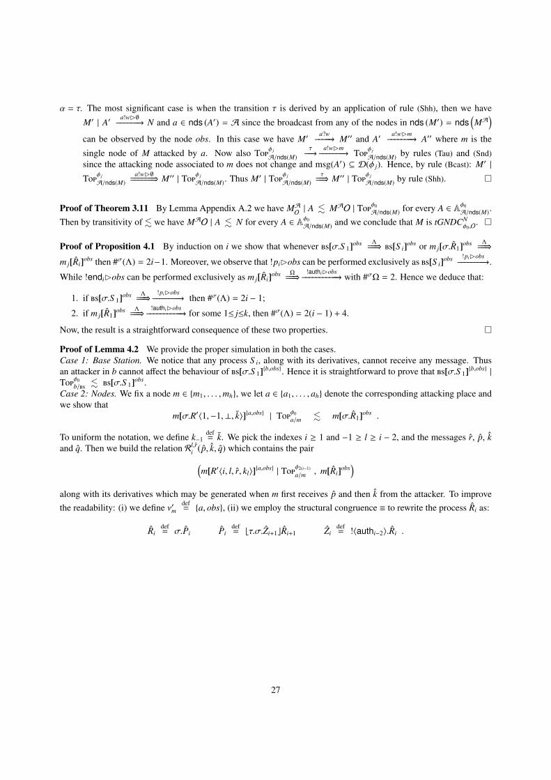
α = τ. The most significant case is when the transition τ is derived by an application of rule (Shh), then we have

M′ | A′a!wB∅−−−−−−−→ N and a ∈ nds (A′) = A since the broadcast from any of the nodes in nds (M′) = nds

(MA)

can be observed by the node obs. In this case we have M′a?w−−−−−→ M′′ and A′

a!wBm−−−−−−−−→ A′′ where m is the

single node of M attacked by a. Now also Tφ j

A/nds(M)τ−−−→

a!wBm−−−−−−−−→ Tφ j

A/nds(M) by rules (Tau) and (Snd)since the attacking node associated to m does not change and msg(A′) ⊆ D(φ j). Hence, by rule (Bcast): M′ |

Tφ j

A/nds(M)a!wB∅=======⇒ M′′ | Tφ j

A/nds(M). Thus M′ | Tφ j

A/nds(M)τ===⇒ M′′ | Tφ j

A/nds(M) by rule (Shh).

Proof of Theorem 3.11 By Lemma Appendix A.2 we have MAO| A . MAO | Tφ0

A/nds(M) for every A ∈ Aφ0A/nds(M).

Then by transitivity of . we have MAO | A . N for every A ∈ Aφ0A/nds(M) and we conclude that M is tGNDCN

φ0,O.

Proof of Proposition 4.1 By induction on i we show that whenever [σ.S 1]obs Λ===⇒ [S i]obs or m j[σ.R1]obs Λ

===⇒

m j[Ri]obs then #σ(Λ) = 2i−1. Moreover, we observe that !piBobs can be performed exclusively as [S i]obs !piBobs−−−−−−−−−→.

While !endiBobs can be performed exclusively as m j[Ri]obs Ω===⇒

!authiBobs−−−−−−−−−−−→ with #σΩ = 2. Hence we deduce that:

1. if [σ.S 1]obs Λ===⇒

!piBobs−−−−−−−−−→ then #σ(Λ) = 2i − 1;

2. if m j[R1]obs Λ===⇒

!authiBobs−−−−−−−−−−−→ for some 1≤ j≤k, then #σ(Λ) = 2(i − 1) + 4.

Now, the result is a straightforward consequence of these two properties.

Proof of Lemma 4.2 We provide the proper simulation in both the cases.Case 1: Base Station. We notice that any process S i, along with its derivatives, cannot receive any message. Thusan attacker in b cannot affect the behaviour of [σ.S 1]b,obs. Hence it is straightforward to prove that [σ.S 1]b,obs |

Tφ0b/ . [σ.S 1]obs.

Case 2: Nodes. We fix a node m ∈ m1, . . . ,mh, we let a ∈ a1, . . . , ah denote the corresponding attacking place andwe show that

m[σ.R′〈1,−1,⊥, k〉]a,obs | Tφ0a/m . m[σ.R1]obs .

To uniform the notation, we define k−1def= k. We pick the indexes i ≥ 1 and −1 ≥ l ≥ i − 2, and the messages r, p, k

and q. Then we build the relation Rl,ri (p, k, q) which contains the pair(

m[R′〈i, l, r, kl〉]a,obs | Tφ2(i−1)

a/m , m[Ri]obs)

along with its derivatives which may be generated when m first receives p and then k from the attacker. To improvethe readability: (i) we define ν′m

def= a, obs, (ii) we employ the structural congruence ≡ to rewrite the process Ri as:

Ridef= σ.Pi Pi

def= bτ.σ.Zi+1cRi+1 Zi

def= !〈authi−2〉.Ri .

27

Then we define

Rl,ri (p, k, q) def

= (

m[R′〈i, l, r, kl〉]ν′m | Tφ2i−1

a/m , m[Ri]obs),(

m[R′〈i, l, r, kl〉]ν′m | a[!〈p〉.Tφ2i−1 ]m, m[Ri]obs

),(

m[σ.P′〈i, l, p, r, kl〉]ν′m | Tφ2i−1

a/m , m[Ri]obs),(

m[σ.P′〈i, l, p, r, kl〉]ν′m | a[!〈p〉.Tφ2i−1 ]m, m[Ri]obs

),(

m[P′〈i, l, p, r, kl〉]ν′m | Tφ2i

a/m, m[Pi]obs),(

m[P′〈i, l, p, r, kl〉]ν′m | a[!〈k〉.Tφ2i ]

m, m[Pi]obs),(

m[T ′〈i, l, p, r, kl, k〉]ν′m | Tφ2i

a/m, m[Pi]obs),(

m[T ′〈i, l, p, r, kl, k〉]ν′m | a[!〈k〉.Tφ2i ]

m, m[Pi]obs),(

m[Q′〈i, l, r, kl〉]ν′m | Tφ2i

a/m, m[Pi]obs) ,(

m[Q′〈i, l, r, kl〉]ν′m | a[!〈k〉.Tφ2i ]

m, m[Pi]obs) ,(

m[Z′〈i+1, i−1, p, r, ki−1〉]ν′m | Tφ2i+1

a/m , m[Zi+1]obs),(

m[Z′〈i+1, i−1, p, r, ki−1〉]ν′m | a[!〈q〉.Tφ2i+1 ]m, m[Zi+1]obs

) .

and we show that the required simulation is(

m[σ.R′〈1,−1,⊥, k〉]a,obs | Tφ0a/m , m[σ.R1]obs ) ∪ R, where the relation

R is defined asR

def=⋃i≥1

⋃−1 ≤ l ≤ i−2r ∈ D(φ2(i−2))

⋃p ∈ D(φ2i−1)k ∈ D(φ2i)

q ∈ D(φ2i+1)

Rl,ri(p, k, q

)

We outline the most significant cases. We omit input actions since the environment contains exclusively the node obswhich cannot transmit, thus all input actions can be derived just by combining rules (RcvEnb) and (RcvPar). We alsoomit τ-actions generated by internal choices of the attacker.In the pair

(m[R′〈i, l, r, kl〉]ν

′m | Tφ2i−1

a/m , m[Ri]obs ) we have a significant action:

• m[R′〈i, l, r, kl〉]ν′m | Tφ2i−1

a/mσ−−−→ m[Q′〈i, l, r, kl〉]ν

′m | Tφ2i

a/m, where m does not receive anything. Then m[Ri]obs σ===⇒

m[Pi]obs.

In the pair(

m[R′〈i, l, r, kl〉]ν′m | a[!〈p〉.Tφ2i−1 ]m, m[Ri]obs ) we have two significant actions:

• m[R′〈i, l, r, kl〉]ν′m | a[!〈 p〉.Tφ2i−1 ]m τ

−−−→ m[σ.P′〈i, l, p, r, kl〉]ν′m | Tφ2i−1

a/m , where m receives p from the attacker.Then m[Ri]obs ==⇒ m[Ri]obs.

• m[R′〈i, l, r, kl〉]ν′m | a[!〈p〉.Tφ2i−1 ]m τ

−−−→ m[R′〈i, l, r, kl〉]ν′m | Tφ2i−1

a/m , where p gets lost. Then m[Ri]obs ==⇒ m[Ri]obs.

In the pair(

m[σ.P′〈i, l, p, r, kl〉]ν′m | Tφ2i−1

a/m , m[Ri]obs ) we have just a significant action:

• m[σ.P′〈i, l, p, r, kl〉]ν′m | Tφ2i−1

a/mσ−−−→ m[P′〈i, l, p, r, kl〉]ν

′m | Tφ2i

a/m. Then the second network replies with

m[Ri]obs σ===⇒ m[Pi]obs.

In the pair(

m[P′〈i, l, p, r, kl〉]ν′m | Tφ2i

a/m, m[Pi]obs ) we have just a significant action:

• m[P′〈i, l, p, r, kl〉]ν′m | Tφ2i

a/mσ−−−→ m[R′〈i+1, l, p, kl〉]ν

′m | Tφ2i+1

a/m , where m does not receive anything. Then

m[Pi]obs σ===⇒ m[Ri+1]obs.

In the pair(

m[P′〈i, l, p, r, kl〉]ν′m | a[!〈k〉.Tφ2i ]

m, m[Pi]obs ) we have two significant actions:

28

• m[P′〈i, l, p, r, kl〉]ν′m | a[!〈k〉.Tφ2i ]

m τ−−−→ m[T ′〈i, l, p, r, kl, k〉]ν

′m | Tφ2i

a/m, where m receives k. Then the secondnetwork replies with m[Pi]obs ==⇒ m[Pi]obs.

• m[P′〈i, l, p, r, kl〉]ν′m | a[!〈k〉.Tφ2i ]

m τ−−−→ m[P′〈i, l, p, r, kl〉]ν

′m | Tφ2i

a/m, where k gets lost. The second networkreplies with m[Pi]obs ==⇒ m[Pi]obs.

In the pair(

m[T ′〈i, l, p, r, kl, k〉]ν′m | Tφ2i

a/m, m[Pi]obs ) we have three significant actions:

• m[T ′〈i, l, p, r, kl, k〉]ν′m | Tφ2i

a/mσ−−−→ m[Z′〈i+1, i−1, p, r, ki−1〉]ν

′m | Tφ2i+1

a/m where m checks that kl = F i−1−l(h)

and authenticates r = pi−1. Then m[Pi]obs σ===⇒ m[Zi+1]obs.

• m[T ′〈i, l, p, r, kl, k〉]ν′m | Tφ2i

a/mσ−−−→ m[R′〈i+1, i−1, p, ki−1〉]ν

′m | Tφ2i+1

a/m where m checks that kl = F i−l(h) without

but it does not authenticate r. Then m[Pi]obs σ===⇒ m[Ri+1]obs.

• m[T ′〈i, l, p, r, kl, k〉]ν′m | Tφ2i

a/mσ−−−→ m[R′〈i+1, l, p, kl〉]ν

′m | Tφ2i+1

a/m where m verifies kl , F i−l(h). Then again

m[Pi]obs σ===⇒ m[Ri+1]obs by timeout.

In the pair(

m[Q′〈i, l, r, kl〉]ν′m | Tφ2i

a/m, m[Pi]obs ) we have a significant action

• m[Q′〈i, l, r, kl〉]ν′m | Tφ2i

a/mσ−−−→ m[R〈i+1, l, r, kl〉]ν

′m | Tφ2i+1

a/m , where m does not receive anything and thus

performs a timeout. Then m[Pi]obs σ===⇒ m[Ri+1]obs.

In the pair(

m[Q′〈i, l, r, kl〉]ν′m | a[!〈k〉.Tφ2i ]

m, m[Pi]obs ) the first network can perform two significant actions

• m[Q′〈i, l, r, kl〉]ν′m | a[!〈k〉.Tφ2i ]

m τ−−−→ m[T 〈i, l, r, r, kl, k〉]ν

′m | Tφ2i

a/m, where m receives k. Then the secondnetwork replies m[Pi]obs ==⇒ m[Pi]obs.

• m[Q′〈i, l, r, kl〉]ν′m | a[!〈k〉.Tφ2i ]

m τ−−−→ m[R〈i+1, l, r, kl〉]ν

′m | Tφ2i

a/m, where k gets lost. Then the second networkreplies m[Pi]obs ==⇒ m[Pi]obs.

Proof of Proposition 5.1 Similar to that of Proposition 4.1.

Proof of Theorem 5.2 The system (LEAP′+)A | A admits the following computation:

m[σ.S 1]νm | r[σ.R′]νr | A σ−−−→

m[S 1]νm | r[R′]νr | a[X]νa | b[σ.X]νb!hello1Bobs−−−−−−−−−−−−→

m[σ.P]νm | r[R′]νr | a[σ.!〈hello1〉.nil]νa | b[σ.X]νb σ−−−→

m[P]νm | r[σ.R′]νr | a[!〈hello1〉.nil]νa | b[X]νb τ−−−→

m[hello1/qP1]νm | r[σ.R′]νr | a[nil]νa | b[σ.!〈hello1〉.nil]νb σ−−−→

m[S 2]νm | r[R′]νr | a[nil]νa | b[!〈hello1〉.nil]νb τ−−−→

m[S 2]νm | r[σ.!〈q1〉.R8′]νr | a[nil]νa | b[nil]νb!hello2Bobs−−−−−−−−−−−−→

m[σ.P]νm | r[σ.!〈q1〉.R8′]νr | a[nil]νa | b[nil]νb σ−−−→

m[P]νm | r[!〈q1〉.R8′]νr | a[nil]νa | b[nil]νb!q1Bobs−−−−−−−−−→

m[q1/qP1]νm | r[R8′]νr | a[nil]νa | b[nil]νb σ−−−→

m[S 3]νm | r[!〈end1〉.nil]νr | a[nil]νa | b[nil]νb!end1Bobs−−−−−−−−−−−→

Then agreement is not reached.

29

Proof of Lemma 5.4 We prove this lemma by showing the appropriate simulations.Case 1: Sender. We define ν′m = a, obs. We need to prove m[σ.S 1]ν

′m | Tφ0

a/m . m[σ.S 1]obs. Thus we fix anindex i = 1, 2, . . ., we pick the messages q′ ∈ D(φ2i−1) and q ∈ D(φ2i), and we build the relation Ri

(q′, q)

containing(m[S ′′i ]ν

′m | Tφ2i−1

a/m , m[S i]obs ) along with its derivatives which may be generated when m receives q from the attacker.

Ri(q′, q) def=

(m[S ′′i ]ν

′m | Tφ2i−1

a/m , m[S i]obs),(

m[S ′′i ]ν′m | a[!〈q′〉.Tφ2i−1 ]m, m[S i]obs

),(

m[σ.P′′]ν′m | Tφ2i−1

a/m , m[σ.⌊τ.σ.!〈authi〉.nil

⌋S i+1]obs

),(

m[σ.P′′]ν′m | a[!〈q′〉.Tφ2i−1 ]m, m[σ.

⌊τ.σ.!〈authi〉.nil

⌋S i+1]obs

),(

m[P′′]ν′m | Tφ2i

a/m, m[⌊τ.σ.!〈authi〉.nil

⌋S i+1]obs

),(

m[P′′]ν′m | a[!〈q〉.Tφ2i ]

m, m[⌊τ.σ.!〈authi〉.nil

⌋S i+1]obs

),(

m[q/qP1′′]ν′m | Tφ2i

a/m, m[⌊τ.σ.!〈authi〉.nil

⌋S i+1]obs

),(

m[q/qP1′′]ν′m | a[!〈q〉.Tφ2i ]

m, m[⌊τ.σ.!〈authi〉.nil

⌋S i+1]obs

),(

m[!〈authi〉.nil]ν′m | Tφ2i+1

a/m , m[!〈authi〉.nil]obs) .

Moreover, it is straightforward to prove that there exists a simulation Ri containing the pair(

m[!〈authi〉.nil]ν′m |

Tφ2i+1a/m , m[!〈authi〉.nil]obs ).Then we show that the required simulation is given by the following relation

Rdef=

m[σ.S 1]ν′m | Tφ0

a/m,m[σ.S 1]obs∪⋃i≥1

(Ri ∪

⋃q′ ∈ D(φ2i−1)q ∈ D(φ2i)

Ri(q′, q)).

As done for Lemma 4.2, we outline the most significant cases.In the pair

(m[S ′′i ]ν

′m | Tφ2i−1

a/m , m[S i]obs ) we have a significant action:

• m[S ′′i ]ν′m | Tφ2i−1

a/m!helloiBobs−−−−−−−−−−−→ m[σ.P′′]ν

′m | Tφ2i−1

a/m , where m broadcasts the packet helloi. Then second network

answers with m[S i]obs !helloiBobs===========⇒ m[σ.

⌊τ.σ.!〈authi〉.nil

⌋S i+1]obs.

In the pair(

m[σ.P′′]ν′m | Tφ2i−1

a/m ,m[σ.⌊τ.σ.!〈authi〉.nil

⌋S i+1]obs ) we have a significant action:

• m[σ.P′′]ν′m | Tφ2i−1

a/mσ−−−→ m[P′′]ν

′m | Tφ2i

a/m. Then m[σ.⌊τ.σ.!〈authi〉.nil

⌋S i+1]obs σ

===⇒ m[⌊τ.σ.!〈authi〉.nil

⌋S i+1]obs.

In the pair(

m[P′′]ν′m | Tφ2i

a/m, m[⌊τ.σ.!〈authi〉.nil

⌋S i+1]obs ) we have a significant action:

• m[P′′]ν′m | Tφ2i

a/mσ−−−→ m[S ′′i+1]ν

′m | Tφ2i+1

a/m , where m does not receive anything and performs a timeout. Then

m[⌊τ.σ.!〈authi〉.nil

⌋S i+1]obs σ

===⇒ m[S i+1]obs.

In the pair(

m[P′′]ν′m | a[!〈q〉.Tφ2i ]

m, m[⌊τ.σ.!〈authi〉.nil

⌋S i+1]obs ) we consider two actions:

• m[P′′]ν′m | a[!〈q〉.Tφ2i ]

m τ−−−→ m[q/qP1′′]ν

′m | Tφ2i

a/m, where m receives q. Then the second network repliesm[⌊τ.σ.!〈authi〉.nil

⌋S i+1]obs ==⇒ m[

⌊τ.σ.!〈authi〉.nil

⌋S i+1]obs.

• m[P′′]ν′m | a[!〈q〉.Tφ2i ]

m τ−−−→ m[P′′]ν

′m | Tφ2i

a/m, where q gets lost. Then m[⌊τ.σ.!〈authi〉.nil

⌋S i+1]obs ==⇒

m[⌊τ.σ.!〈authi〉.nil

⌋S i+1]obs.

In(

m[q/qP1′′]ν′m | Tφ2i

a/m, m[⌊τ.σ.!〈authi〉.nil

⌋S i+1]obs ) we have two significant actions:

30

• m[q/qP1′′]ν′m | Tφ2i

a/mσ−−−→ m[!〈authi〉.nil]ν

′m | Tφ2i+1

a/m , where m verifies that q refers to the nonce ni. Then

m[⌊τ.σ.!〈authi〉.nil

⌋S i+1]obs σ

===⇒ m[!〈authi〉.nil]obs.

• m[q/qP1′′]ν′m | Tφ2i

a/mσ−−−→ m[S ′′i+1]ν

′m | Tφ2i+1

a/m , where m verifies that q does not refer to ni, or it finds out that q

is corrupted. Then m[⌊τ.σ.!〈authi〉.nil

⌋S i+1]obs σ

===⇒ m[S i+1]obs.

Case 2: Receiver. To show that r[σ.R]b | Tφ0b/r . r[Tick]∅ we define the following relation:

Rdef= (M, r[Tick]∅) such that r[σ.R]b | Tφ0

b/rΛ===⇒ M .

We first note that for every (M, r[Tick]∅) ∈ R we have Env (M) = ∅. Thus the most significant actions can only beM

τ−−−→ or M

σ−−−→ or input actions that can be derived without applying rule (Rcv). Then it is straightforward to prove

that R is a simulation.

Proof of Proposition 6.1 Similar to that of Proposition 4.1.

Proof of Theorem 6.2 The system(LiSP′

)A| A admits the following computation:

m[σ.Z′]νm | [σ.L0]ν | A σ−−−→

m[Z′]νm | [L0]ν | a[σ2.X]νa∣∣∣ b[σ.X]νb !rBobs

−−−−−−−−→

m[σ.b?(q).T ′cZ′]νm | [r/rI1]ν | a[σ2.X]νa∣∣∣ b[σ.X]νb σ

−−−→

m[b?(q).T ′cZ′]νm | [!〈q1〉.σ.L1]ν | a[σ.X]νa | b[X]νb!q1Bobs−−−−−−−−−→

m[b?(q).T ′cZ′]νm | [σ.L1]ν | a[σ.X]νa | b[σ.!〈q1〉.nil]νb σ−−−→

m[Z′]νm | [L1]ν | a[X]νa | b[!〈q1〉.nil]νb τ−−−→

m[Z′]νm | [q1/rI2]ν | a[σ.!〈q1〉.nil]νa | b[nil]νb !rBobs−−−−−−−−→

m[σ.b?(q).T ′cZ′]νm | [q1/rI2]ν | a[σ.!〈q1〉.nil]νa | b[nil]νb σ−−−→

m[b?(q).T ′cZ′]νm | [σ.L2]ν | a[!〈q1〉.nil]νa | b[nil]νb τ−−−→

m[q1/qT ′]νm | [σ.L2]ν | a[nil]νa | b[nil]νb σ−−−→

m[σ.!〈auth1〉.R(k2, ks+1, s − 1)]νm | [L2]ν | a[nil]νa | b[nil]νb σ−−−→

m[!〈auth1〉.R(k2, ks+1, s − 1)]νm | [σ.L3]ν | a[nil]νa | b[nil]νb!auth1Bobs−−−−−−−−−−−→

Then m signals the correct reconfiguration based on an old packet.

31