program for analysis and visualization of large...
TRANSCRIPT

PajekProgram for Analysis and
Visualization of Large Networks
Reference ManualList of commands with short explanation
version 2.05
Vladimir Batagelj and Andrej Mrvar
Ljubljana, September 24, 2011

c©1996, 2011 V. Batagelj, A. Mrvar. Free for noncommercial use.
PdfLaTex version October 1, 2003
Vladimir BatageljDepartment of Mathematics, FMFUniversity of Ljubljana, Slovenia
http://vlado.fmf.uni-lj.si/
Andrej MrvarFaculty of Social SciencesUniversity of Ljubljana, Slovenia
http://mrvar.fdv.uni-lj.si/

Contents1 Pajek 3
2 Data objects 6
3 Main Window Tools 83.1 File . . . . . . . . . . . . . . . . . . . . . . . . . . . . . . . . . 83.2 Net . . . . . . . . . . . . . . . . . . . . . . . . . . . . . . . . . 133.3 Nets . . . . . . . . . . . . . . . . . . . . . . . . . . . . . . . . . 303.4 Operations . . . . . . . . . . . . . . . . . . . . . . . . . . . . . 333.5 Partition . . . . . . . . . . . . . . . . . . . . . . . . . . . . . . 433.6 Partitions . . . . . . . . . . . . . . . . . . . . . . . . . . . . . . 443.7 Vector . . . . . . . . . . . . . . . . . . . . . . . . . . . . . . . . 453.8 Vectors . . . . . . . . . . . . . . . . . . . . . . . . . . . . . . . 463.9 Permutation . . . . . . . . . . . . . . . . . . . . . . . . . . . . 473.10 Permutations . . . . . . . . . . . . . . . . . . . . . . . . . . . . 483.11 Cluster . . . . . . . . . . . . . . . . . . . . . . . . . . . . . . . 483.12 Hierarchy . . . . . . . . . . . . . . . . . . . . . . . . . . . . . . 483.13 Options . . . . . . . . . . . . . . . . . . . . . . . . . . . . . . . 493.14 Info . . . . . . . . . . . . . . . . . . . . . . . . . . . . . . . . . 523.15 Tools . . . . . . . . . . . . . . . . . . . . . . . . . . . . . . . . 53
4 Draw Window Tools 564.1 Main Window Draw Tool . . . . . . . . . . . . . . . . . . . . . . 564.2 Layout . . . . . . . . . . . . . . . . . . . . . . . . . . . . . . . 564.3 Layers . . . . . . . . . . . . . . . . . . . . . . . . . . . . . . . . 584.4 GraphOnly . . . . . . . . . . . . . . . . . . . . . . . . . . . . . 604.5 Previous . . . . . . . . . . . . . . . . . . . . . . . . . . . . . . . 604.6 Redraw . . . . . . . . . . . . . . . . . . . . . . . . . . . . . . . 604.7 Next . . . . . . . . . . . . . . . . . . . . . . . . . . . . . . . . . 604.8 ZoomOut . . . . . . . . . . . . . . . . . . . . . . . . . . . . . . 604.9 Options . . . . . . . . . . . . . . . . . . . . . . . . . . . . . . . 604.10 Export . . . . . . . . . . . . . . . . . . . . . . . . . . . . . . . 644.11 Spin . . . . . . . . . . . . . . . . . . . . . . . . . . . . . . . . . 674.12 Move . . . . . . . . . . . . . . . . . . . . . . . . . . . . . . . . 674.13 Info . . . . . . . . . . . . . . . . . . . . . . . . . . . . . . . . . 68
5 Exports to EPS/SVG/X3D/VRML 695.1 Defaults . . . . . . . . . . . . . . . . . . . . . . . . . . . . . . . 695.2 Parameters in EPS, SVG, X3D, and VRML Defaults Window . . . 69
1

5.3 Exporting pictures to EPS/SVG – defining parameters in input file 735.4 Using Unicode in Pajek’s pictures . . . . . . . . . . . . . . . . . 77
6 Using Macros in Pajek 806.1 What is a Macro? . . . . . . . . . . . . . . . . . . . . . . . . . . 806.2 How to record a Macro? . . . . . . . . . . . . . . . . . . . . . . 806.3 How to execute the Macro? . . . . . . . . . . . . . . . . . . . . . 806.4 Example . . . . . . . . . . . . . . . . . . . . . . . . . . . . . . . 806.5 List of macros available in installation file . . . . . . . . . . . . . 81
6.5.1 Macros prepared for genealogies and other acyclic networks 816.5.2 Macros prepared for computing derived kinship relations . 82
6.6 Repeating last command . . . . . . . . . . . . . . . . . . . . . . 82
7 Blockmodeling in Pajek 847.1 MDL files . . . . . . . . . . . . . . . . . . . . . . . . . . . . . . 847.2 Examples of MDL files . . . . . . . . . . . . . . . . . . . . . . . 86
7.2.1 Regular blocks . . . . . . . . . . . . . . . . . . . . . . . 867.2.2 Diagonal blocks (clustering) . . . . . . . . . . . . . . . . 867.2.3 Acyclic model (up) . . . . . . . . . . . . . . . . . . . . . 867.2.4 Acyclic model with symmetric clusters (down) . . . . . . 867.2.5 Center-Periphery . . . . . . . . . . . . . . . . . . . . . . 877.2.6 Regular path . . . . . . . . . . . . . . . . . . . . . . . . 877.2.7 Regular chain . . . . . . . . . . . . . . . . . . . . . . . . 877.2.8 2-mode ’standard model’ for Davis.net . . . . . . . . . . 88
8 Colors in Pajek 89
9 Citing Pajek 91
2

Pajek– Manual 3
1 Pajek
Pajek is a program, for Windows, for analysis and visu-alization of large networks having some thousands or evenmillions of vertices. In Slovenian language the word pa-jek means spider. The latest version of Pajek is freelyavailable, for noncommercial use, at its home page:
http://vlado.fmf.uni-lj.si/pub/networks/pajek/
We started the development of Pajek in November 1996. Pajek is im-plemented in Delphi (Pascal). Some procedures were contributed by Matjaz Za-versnik.
The main motivation for development of Pajek was the observation thatthere exist several sources of large networks that are already in machine-readableform. Pajek should provide tools for analysis and visualization of such net-works: collaboration networks, organic molecule in chemistry, protein-receptorinteraction networks, genealogies, Internet networks, citation networks, diffusion(AIDS, news, innovations) networks, data-mining (2-mode networks), etc. Seealso collection of large networks at:
http://vlado.fmf.uni-lj.si/pub/networks/data/
The design of Pajek is based on our previous experiences gained in devel-opment of graph data structure and algorithms libraries Graph and X-graph, col-lection of network analysis and visualization programs STRAN, RelCalc, Draw,Energ, and SGML-based graph description markup language NetML.
http://vlado.fmf.uni-lj.si/pub/networks/default.htm
Figure 1: Pajek/Spider
V. Batagelj and A. Mrvar Pajek 2.05 / September 24, 2011

4 Pajek– Manual
cut-out
reduction
local
glo
ba
l
hierarchy
contextinter-links
Figure 2: Approaches to deal with large networks
The main goals in the design of Pajek are:
• to support abstraction by (recursive) decomposition of a large network intoseveral smaller networks that can be treated further using more sophisticatedmethods;
• to provide the user with some powerful visualization tools;
• to implement a selection of efficient (subquadratic) algorithms for analysisof large networks.
With Pajek we can: find clusters (components, neighbourhoods of ‘impor-tant’ vertices, cores, etc.) in a network, extract vertices that belong to the sameclusters and show them separately, possibly with the parts of the context (detailedlocal view), shrink vertices in clusters and show relations among clusters (globalview).
Besides ordinary (directed, undirected, mixed) networks Pajek supports alsomulti-relational networks, 2-mode networks (bipartite (valued) graphs – networksbetween two disjoint sets of vertices), and temporal networks (dynamic graphs –networks changing over time).
V. Batagelj and A. Mrvar Pajek 2.05 / September 24, 2011
Pajek– Manual 5
Figure 3: Pajek textbook
This manual provides short explanations of all procedures implemented in thelast version of Pajek. The novice users we advise to read the Pajek textbook[31]
de Nooy W., Mrvar A., Batagelj V. (2002) Exploratory Social Net-work Analysis With Pajek. Structural Analysis in the Social Sci-ences 27, Cambridge University Press, 2005.
For an overview of network analysis with Pajek see the NICTA workshop slides[5].
V. Batagelj and A. Mrvar Pajek 2.05 / September 24, 2011

6 Pajek– Manual
2 Data objectsIn Pajek six types of objects are used:
Figure 4: Pajek’s Main Window
1. Networks – main objects (vertices and lines). Default extension: .net.Network can be presented on input file in different ways:
• using arcs/edges (e.g. 1 2 – line from 1 to 2)• using arcslists/edgeslists (e.g. 1 2 3 – line from 1 to 2 and from 1 to 3)• matrix format• UCINET, GEDCOM, chemical formats. . .
Additional information for network drawing can be included in input file aswell. This is explained in the section Exports to EPS/SVG/VRML.
2. Partitions – they tell for each vertex to which class vertex belong. Defaultextension: .clu.
3. Permutations – reordering of vertices. Default extension: .per.
4. Clusters – subset of vertices (e.g. one class from partition). Default exten-sion: .cls.
5. Hierarchies – hierarchically ordered vertices. Example:
Rootg1 g2
g11 g12 v5,v6,v7v1,v2 v3,v4
V. Batagelj and A. Mrvar Pajek 2.05 / September 24, 2011

Pajek– Manual 7
Root has two subgroups – g1 and g2. g2 is a leaf – cluster with verticesv5,v6 and v7. g1 has two subgroups – g11 and g12. . . Default extension:.hie.
6. Vectors – they tell for each vertex some numerical property (real number).Default extension: .vec.
By double clicking on selected network, partition,... you can show the objecton screen.
The procedures in Pajek’s main window (see Figure 4) are organized accord-ing to the types of data objects they use as input.
Permutations, partitions and vectors can be used to store properties of verticesmeasured in different scales: ordered, nominal (categorical) and numeric.
Figure 5: Spider web; Photo: Vladimir Batagelj.
V. Batagelj and A. Mrvar Pajek 2.05 / September 24, 2011

8 Pajek– Manual
3 Main Window Tools
3.1 File
Input/Output manipulation with the six data objects.
• Network – N
– Read – Read network from Ascii file.
– Edit – Edit network. Choose vertex, show its neighbors and then:
∗ add new lines to/from selected vertex (by left mouse double click-ing on Newline);∗ delete lines (by left mouse double clicking);∗ change value of line (by single right mouse clicking);∗ subdivide line to two orthogonal lines using new invisible vertex
(by single middle mouse clicking).
– Save – Save selected network to Ascii file.If network represents Ore graph with the following five relations (arcs):1. Wi→Hu, 2. Mo→Da, 3. Mo→So, 4. Fa→Da, 5. Fa→Soit can be stored as GEDCOM file.The other possibility is Pajek Ore graph: 1.Fa→Ch, 2.Mo→Ch, 3.Hu-Wi (edge), or 1.Pa→Ch, 3.Hu-Wi (edge).
– Export Matrix to EPS – write matrix in EPS format:
∗ Original – using default numbering (for 1-mode and 2-mode net-works).∗ Using Permutation – using current permutation. Additionally
lines can be drawn to divide different classes defined by selectedpartition. Option can be used for 1-mode and 2-mode networks.∗ Using Partition – using current partition. In the text window
number and density of lines among classes (and vertices in se-lected two classes) are displayed. Additionally matrix is exportedto EPS where density is expressed using shadowing:1. Structural – Densities are normalized according to maxi-
mum possible number of lines among classes (suitable fordense networks).
2. Delta – Densities are normalized according to vertices havingthe highest number of input and output neighbors in classes(suitable for sparse networks).
V. Batagelj and A. Mrvar Pajek 2.05 / September 24, 2011

Pajek – Manual 9
∗ Diamonds for Negative Values, Circles for 0 – Squares are usedfor posititive values, diamonds for negative and circles for value0 (useful for black and white printing).∗ Diamonds, Circles and Lines in GreyScale – Diamonds, circles
and dividing lines are drawn in greyscale (not in red, green andblue).∗ Labels on Top/Right – Labels are written on the top and on the
right of the matrix - suitable for longer labels.∗ Only Black Borders – All squares in matrix have black borders,
otherwise dark squares will have white and light squares will haveblack borders.∗ Thick Boundary Line – Use thicker line for dividing clusters.∗ Large Squares/Diamonds/Circles – Use larger or smaller squares,
diamonds, and circles.∗ Use Partition Colors for Vertex Labels – Labels of vertices are
displayed using partition colors.
– Change Label of selected network.
– Dispose selected network from memory.
• Time Events Network – N
– Read Time Events – Read time network described using time events.See Table 1.List of properties s can be empty as well. If several edges (arcs) canconnect two vertices, additional tag like :k (k-th line) must be given todetermine to which line the command applies. E.g. command HE:314 37 results in hiding the third edge connecting vertices 14 and 37.Example of time network described using time events:
*Vertices 3*EventsTI 1AV 2 "b"TE 3HV 2TI 4AV 3 "e"TI 5AV 1 "a"TI 6AE 1 3 1TI 7SV 2AE 1 2 1
V. Batagelj and A. Mrvar Pajek 2.05 / September 24, 2011

10 Pajek – Manual
Table 1: List of time events.
Event ExplanationTI t initial events – following events happen when
time point t startsTE t end events – following events happen when
time point t is finishedAV vns add vertex v with label n and properties sHV v hide vertex vSV v show vertex vDV v delete vertex vAA uvs add arc (u,v) with properties sHA uv hide arc (u,v)SA uv show arc (u,v)DA uv delete arc (u,v)AE uvs add edge (u:v) with properties sHE uv hide edge (u:v)SE uv show edge (u:v)DE uv delete edge (u:v)CV vs change vertex property – change property of vertex v to sCA uvs change arc property – change property of arc (u,v) to sCE uvs change edge property – change property of edge (u:v) to sCT uv change type – change (un)directedness of line (u,v)CD uv change direction of arc (u,v)PE uvs replace pair of arcs (u,v) and (v,u) by single edge (u:v)
with properties sAP uvs add pair of arcs (u,v) and (v,u)
with properties sDP uv delete pair of arcs (u,v) and (v,u)EP uvs replace edge (u:v) by pair of arcs (u,v) and (v,u)
with properties s
V. Batagelj and A. Mrvar Pajek 2.05 / September 24, 2011

Pajek– Manual 11
TE 7DE 1 2DV 2TE 8DE 1 3TE 10HV 1TI 12SV 1TE 14DV 1
See also other possibility: description of time network using time in-tervals.
– Save – Save time network in time events format.
• Partition – C
– Read partition from Ascii file.
– Edit partition (put vertices to classes).
– Save selected partition to Ascii file.
– Change Label of selected partition.
– Dispose selected partition from memory.
• Permutation – P
– Read permutation from Ascii file.
– Edit permutation (interchange positions of two vertices).
– Save selected permutation to Ascii file.
– Change Label of selected permutation.
– Dispose selected permutation from memory.
• Cluster – S (list of selected vertices)
– Read cluster from Ascii file.
– Edit cluster (add and delete vertices).
– Save selected cluster to Ascii file.
– Change Label of selected cluster.
– Dispose selected cluster from memory.
• Hierarchy – H
– Read hierarchy from Ascii file.
V. Batagelj and A. Mrvar Pajek 2.05 / September 24, 2011

12 Pajek– Manual
– Edit hierarchy (change types and names of nodes, or show vertices(and subtree) belonging to selected node). Nodes can be pushed upand down within hierarcy.
– Save selected hierarchy to Ascii file.
– Change Label of selected hierarchy.
– Dispose selected hierarchy from memory.
• Vector – V
– Read vector from Ascii file.
– Edit vector (change components of vector).
– Save selected vector(s) to Ascii file. If cluster representing vector id’sis present, all vectors with corresponding id numbers will be saved tothe same output file. Vector’s id can be added to cluster by pressingV on the selected vector (empty cluster should be created first). Allvectors must have the same dimensions.
– Change Label of selected vector.
– Dispose selected vector from memory.
• Pajek Project File – *.paj
– Read Pajek project file (file containing all possible Pajek data ob-jects – networks, partitions, permutations, clusters, hierarchies andvectors).
– Save all currently loaded objects as a Pajek project file.
• Repeat session – During program execution all commands are written tofile *.log. In this way you can repeat any execution by running selectedlog file. If you change in the log file a name of a file to ?, program willask for name when running logfile next time (so you can repeat the samesequence of steps – logfile with different input data). If startup logfile (Pa-jek.log) exists (in the same directory as Pajek.exe), it is automatically exe-cuted every time when Pajek is run.
• Show Report Window – Bring the report window in the front in the casethat it was closed or is not visible.
• Exit program.
V. Batagelj and A. Mrvar Pajek 2.05 / September 24, 2011

Pajek– Manual 13
3.2 NetOperations, for which only a network is needed as input.
• Transform
– Transpose – Transposed network of selected network:
∗ 1-Mode - Change direction of arrows.∗ 2-Mode - Interchange Rows and Cols.
– Remove
∗ Selected Vertices – Remove selected vertices from network.∗ all Edges – Remove all edges from selected network.∗ all Arcs – Remove all arcs from selected network.∗ Multiple Lines – Remove all multiple lines from selected net-
work.1. Sum Values – Values of all deleted lines are added to not
deleted line between corresponding two vertices.2. Number of Lines – Value of line between two vertices in a
new network correspond to the number of lines between thetwo vertices in original network.
3. Min Value – Minimum value of all lines between two verticesis selected.
4. Max Value – Maximum value of all lines between two ver-tices is selected.
5. Single Line – Value of line between two vertices in a newnetwork is 1.
∗ Loops – Remove all loops from selected network.∗ Lines with Value
1. lower than – Remove all lines with value lower than specifiedvalue.
2. higher than – Remove all lines with value higher than speci-fied value.
3. within interval – Remove all lines with values within speci-fied interval.
∗ all Arcs from each Vertex except1. k with Lowest Line Values – Sort lines around vertices in
ascending order according to output line values. Keep onlyselected number of lines with lowest values.
V. Batagelj and A. Mrvar Pajek 2.05 / September 24, 2011

14 Pajek– Manual
2. k with Highest Line Values – Sort lines around vertices indescending order according to output line values. Keep onlyselected number of lines with highest values.
3. keep Lines with Value equal to the k-th Value – Determinewhat to do with lines with value equal to the k-th value (re-move them or not).
∗ Triangle – Remove arcs belonging to lower or upper triangle.
– Add additional vertices, lines or vertices/lines labels to network.
∗ Vertices – Copy network to new network. Dimension can be en-larged for selected number of vertices (additional vertices withoutlines are added).∗ Source and Sink – If network is acyclic, add unique first and last
vertex (new network has two artificial vertices).∗ Default Vertex Labels – Replace current labels of vertices by
default vertices labels (v1, v2...).∗ Vertex Labels from File – Replace the default vertices labels (v1,
v2...) by labels given in a file.∗ Line Labels as Line Values – replace labels of lines (or create
new if there are no) with line values. Number of decimal placesis the same as used in Draw window for marking lines with linevalues.∗ Sibling edges – Add sibling edges to vertices with a common
1. Input – arc-ancestor2. Output – arc-descendant
– Edges→ Arcs – Convert all edges to arcs (in both directions) (makedirected network).
– Arcs→ Edges
∗ All – Convert all arcs to edges (make undirected network).∗ Bidirected only – Convert only arcs in both directions to edges:
1. Sum Values – Value of the new edge is the sum of values ofboth arcs.
2. Min Value – Value of the new edge is the smaller of valuesof arcs.
3. Max Value – Value of the new edge is the larger of values ofarcs.
– Bidirected Arcs→ Arc
V. Batagelj and A. Mrvar Pajek 2.05 / September 24, 2011

Pajek– Manual 15
∗ Select Min Value – If there exist bidirected arcs between twovertices retain only the arc with lower value and remove the arcwith higher value. If both values are equal replace both arcs withan edge.∗ Select Max Value – If there exist bidirected arcs between two
vertices retain only the arc with higher value and remove the arcwith lower value. If both values are equal replace both arcs withan edge.
– Line Values – Transformations of line values:
∗ Recode – Display frequency distribution of line values accordingto selected intervals and recode line values in this way.∗ Multiply by a constant.∗ Add Constant to line values.∗ Constant – min or max of line value and selected constant.∗ Absolute line values.∗ Absolute + Sqrt – square root of line values.∗ Truncate – truncated line values.∗ Exp – exponent of line values.∗ Ln – natural logarithm of line values.∗ Power – selected power of line values.∗ Normalize
1. Sum – normalize so that the sum of line values will be 12. Max – normalize so that the maximum line value will be 1
– Reduction
∗ Degree – (Recursively) delete from network all vertices with de-gree lower than selected value (according to Input, Output or Alldegree). Operation can be limited to selected cluster.∗ Hierarchical – Recursively delete from network all vertices that
have only 0 or 1 neighbor. Results: simpler network and hierarchywith deleted vertices. Original network can be later restored (if weforget directions of lines).∗ Subdivisions – Recursively delete from network all vertices that
have exactly 2 neighbors (together with corresponding two lines)and (instead of that) add direct line between these two neighbors.Result is simpler network (for drawing). Original network cannotbe restored!
V. Batagelj and A. Mrvar Pajek 2.05 / September 24, 2011
16 Pajek – Manual
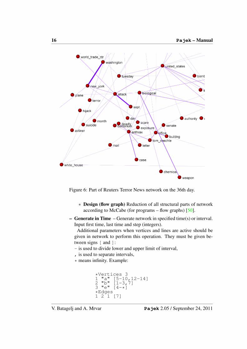
Figure 6: Part of Reuters Terror News network on the 36th day.
∗ Design (flow graph) Reduction of all structural parts of networkaccording to McCabe (for programs – flow graphs) [50].
– Generate in Time – Generate network in specified time(s) or interval.Input first time, last time and step (integers).
Additional parameters when vertices and lines are active should begiven in network to perform this operation. They must be given be-tween signs [ and ]:- is used to divide lower and upper limit of interval,, is used to separate intervals,* means infinity. Example:
*Vertices 31 "a" [5-10,12-14]2 "b" [1-3,7]3 "e" [4-*]*Edges1 2 1 [7]
V. Batagelj and A. Mrvar Pajek 2.05 / September 24, 2011

Pajek– Manual 17
1 3 1 [6-8]
Vertex ’a’ is active from times 5 to 10, and 12 to 14, vertex ’b’ in times1 to 3 and in time 7, vertex ’e’ from time 4 on. Line from 1 to 2 is ac-tive only in time 7, line from 1 to 3 in times 6 to 8.The lines and vertices in a temporal network should satisfy the consis-tency condition: if a line is active in time t then also its end-verticesare active in time t. When generating time slices of a given temporalnetwork only ’consistent’ lines are generated.Note that time records should always be written as last in the rowwhere vertices / lines are defined.See also other possibility of describing time network: description oftime network using time events.
∗ All – Generate all networks in specified times.∗ Only Different – Generate network in specified time only if the
new network will differ in at least one vertex or line from the lastnetwork which was generated.∗ Interval – Generate network with vertices and lines present in
selected interval.
– 1-Mode to 2-Mode – Generate 2-mode network from any network.
– 2-Mode to 1-Mode – Generate an ordinary (1-mode) network from2-mode (affiliation) network. Result is a valued network. To storea 2-mode network in input file use Pajek or Ucinet format (look atDavis.dat from Ucinet dataset).
∗ Rows – Result is a network with relations among row elements(actors). The value of line tells number of common events of thetwo actors.∗ Columns – Result is network with relations among column ele-
ments (events). The value of a line tells number of actors that tookpart in both events.∗ Include Loops – If checked, loops with value telling the total
number of events for each actor (total number of actors for eachevent), are added.∗ Multiple Lines – Generate nonvalued 1-mode network, where
multiple lines among vertices can exist. The label of the gen-erated line corresponds to the label of the event/actor that servedto induce the line. If partition of the same dimension is present,multirelational network can be generated.
V. Batagelj and A. Mrvar Pajek 2.05 / September 24, 2011

18 Pajek– Manual
∗ Normalize 1-Mode – Normalize the obtained 1-Mode network.1-Mode network must be obtained with option include loops check-ed, and multiple lines not checked:
Geoij =aij√aiiajj
Inputij =aijajj
Outputij =aijaii
Minij =aij
min(aii, ajj)
Maxij =aij
max(aii, ajj)
MinDirij ={ aij
aiiaii ≤ ajj
0 otherwise
MaxDirij ={ aij
ajjaii ≤ ajj
0 otherwise
The obtained network is usually not sparse. To make it sparseruse Net/Transform/Remove/lines with value/lower than.∗ Rows=Cols – Transform 2-Mode network with the same subsets
of vertices to 1-Mode network.∗ Cols=0 – Transform 2-Mode network to 1-Mode network by set-
ting number of columns to 0. The result is the same as changingfor example *Vertices 32 18 to *Vertices 32 in inputnetwork file.
– Multiple Relations∗ Extract Relation(s) – Extract one or selected list of relations
from selected multiple relations network.∗ Canonical Numbering – Enumerate relations with sequential num-
bers 1, 2,. . .∗ Generate 3-Mode Network – generate a 3-mode network from
1-mode or 2-mode multirelational network. For each line in mul-tirelational network r: i j v (line from i to j with value v,relation number is r) generate the following three lines (triangle):· 1-mode networks:i N+j v
V. Batagelj and A. Mrvar Pajek 2.05 / September 24, 2011

Pajek– Manual 19
i 2N+r vN+j 2N+r v
· 2-mode networks:i j vi N+M+r vj N+M+r v
where N is cardinality of the first mode and M cardinality of thesecond mode.∗ Line Values − > Relation Numbers – Store line values as rela-
tion numbers (absolute truncated values).∗ Relation Numbers− > Line Values – Store relation numbers as
line values.∗ Change Relation Number - Label – Change selected relation
number to new relation number with corresponding label.
– Sort Lines –
∗ Neighbors around Vertices – For each vertex sort lines con-nected to it in ascending order according to other end-vertex.∗ Line Values – Sort lines in ascending or descending order accord-
ing to line values.
• Random Network – Generate random network of selected dimension
– Total No. of Arcs – Generate random directed network of selecteddimension and given number of arcs.
– Vertices Output Degree – Generate random directed network of se-lected dimension and output degree of each vertex in given range.
– Bernoulli/Poisson – Generate undirected, directed, acyclic, bipartiteor 2-mode random network according to model defined by Bernoulli/ Poisson: each line is selected with the given probability p. Insteadof p, which is for large and sparse networks (very) small number, inPajek a more intuitive average degree d is used. They are connectedwith relations d = 1
n
∑v∈V deg(v) = 2m
nandm = pM where n = |V |,
m = |L| and M is the number of lines in maximal possible network –for example, for undirected graphs M = n(n− 1).
– Scale Free – Generate scale free undirected, directed or acyclic net-work. The procedure is based on a refinement of the model for gener-ating scale free networks, proposed in [55]. At each step of the growtha new vertex and k edges are added to the network N . The endpoints
V. Batagelj and A. Mrvar Pajek 2.05 / September 24, 2011
20 Pajek– Manual
of the edges are randomly selected among all vertices according to theprobability
Pr(v) = αindeg(v)|E|
+ βoutdeg(v)|E|
+ γ1
|V |
where α + β + γ = 1. It is easy to check that∑
v∈V Pr(v) = 1.
– Small World – Generate Small world random network. See [12].
– Extended Model – Generate random network according to extendedmodel defined by Albert and Barabasi [3].
• Partitions – Partitioning Network. Result is a Partition.
– Degree
∗ Input – Number of lines into vertices.∗ Output – Number of lines out of vertices.∗ All – Number of neighbors of vertices.
– Domain – For each vertex compute its domain according to input,output or all neighbors. Results are:
∗ Partition containing size of domain - number of reachable ver-tices.∗ Vector containing the normalized size of domain - normalization
is done by total number of vertices – 1.∗ Vector containing the average distance from/to domain.
Proximity Prestige index can be computed by dividing the normalizedsize of domain by average distance.
– Core – k-core is a subnetwork of given network where each vertex hasat least k neighbors in the same core according to:
∗ Input ... lines coming into vertex.∗ Output ... lines going out of vertex.∗ All ... all neighbors.∗ 2-Mode – core partition of a 2-mode network. Given minimum
degree in first (k1) and minimum degree in second subset (k2)a new partition is generated where 0 means that vertex does notbelong to the core of prespecified k1 and k2, 1 means that vertexbelongs to that core.
V. Batagelj and A. Mrvar Pajek 2.05 / September 24, 2011

Pajek– Manual 21
268256233224853636168 3666948 36917553697150 3767289 3773747 37954363796479
3876286
3891307
39473753954653 3960752
3975286 400008440111734013582 40174164029595
4032470
4077260
408242840837974113647 41183354130502
4149413
4154697
4195916
41981304202791
4229315 4261652
42909054293434 4302352 4330426
43404984349452
43570784361494
4368135
4386007
43870384387039
44002934415470
4419263 4422951
4455443
4456712
4460770 4472293 44725924480117
4502974
4510069
45140444526704
455098145581514583826
46219014630896
4657695
4659502
4695131 47042274709030 4710315 47131974719032
472136747524144770503 4795579 4797228
4820839 483246248775474957349
5016988 50169895122295
5124824 5171469 5283677
5555116
Figure 7: US Patents – Main island ’liquid-crystal display’
V. Batagelj and A. Mrvar Pajek 2.05 / September 24, 2011

22 Pajek– Manual
∗ 2-Mode Review – Given starting values of k1 and k2 the follow-ing list is computed:k1 k2 Rows Cols Compwhere k1 is minimum degree in the first, k2 minimum degree inthe second subset, Rows and Cols are number of vertices in firstand second subset respectivelly and Comp, number of connectedcomponents in network induced by k1 and k2. k1 and k2 are in-cremented until the resulting network is empty.∗ 2-Mode Border – Compute only border values of k1 and k2 for
a given 2-mode network.
– Valued Core – Generalized k-core: Instead of counting lines (neigh-bors) use values of lines. sum of lines or maximum value can be usedwhen computing valued core:Sum valued core of threshold val is a subnetwork of given networkwhere the sum of values of lines to (from) the members of the samecore is at least val.Max valued core of threshold val is a subnetwork of given networkwhere the maximum value of all lines to (from) the members of thesame core is at least val.Threshold values must be given in advance. Two different ways todetermine thresholds:
∗ First Threshold and Step – Select first threshold value and stepin which to increase threshold.∗ Selected Thresholds – Thresholds (increasing numbers) are given
using vector.∗ 2-Mode – valued core (according to line values) partition of a 2-
mode network. Given minimum valued degree in first (k1) andminimum valued degree in second subset (k2) a new partition isgenerated where 0 means that vertex does not belong to the valuedcore of prespecified k1 and k2, 1 means that vertex belongs to thatcore.
Additionally (for 1-mode networks), Input, Output or All valued corescan be used.
– Depth
∗ Acyclic – Partition acyclic network according to depths of ver-tices.∗ Genealogical – Partition network that represents genealogy ac-
cording to layers of vertices.
V. Batagelj and A. Mrvar Pajek 2.05 / September 24, 2011

Pajek– Manual 23
∗ Generational – Partition network that represents genealogy ac-cording to layers of vertices. The same as genealogical partitionbut with less layers.
– p-Cliques Partition network according to p-Cliques (partition to clus-ters where vertices have at least proportion p (number between 0 and1) neighbors inside the cluster.
∗ Strong ... for directed network.∗ Weak ... for undirected network.
– Vertex Labels – Partition vertices with same labels to the same classnumbers (for molecule).
– Vertex Shapes – Partition vertices with same shapes (ellipse, box, dia-mond) to the same class numbers (used in genealogy to show gender).
– Islands – Partition vertices of network with values on lines (weights)to cohesive clusters (weights inside clusters must be larger than weightsto neighborhood): the height of vertex (vector) is defined as the maxi-mum weight of the neighbor lines. Two options:
∗ Line Weights∗ Line Weights [Simple]
New network with only lines constituting islands can be generated ifGenerate Network with Islands is checked.
– Bow-Tie – Partition vertices of directed network (graph structure ofthe web) to the following classes: 1 – LSCC, 2 – IN, 3 – OUT, 4 –TUBES, 5 – TENDRILS, 0 – OTHERS.
– 2-Mode – Partition of vertices of a 2-mode network into two subsets.
– Default Labels Partition – Input is network with default vertex la-bels: e.g., v3, v9,... Result is a partition of selected dimension, wherevertices defined by numbers stored in vertex labels (e.g., 3, 9,...) go tocluster 1, other vertices go to cluster 0.Operation can be used to make other objects (e.g. partitions, vectors,...) compatible with a network, if network is reduced by several oper-ations (e.g. extractions).
• Components
– Strong – Strong Components of selected network.
– Strong-Periodic – Strong Periodic Components of selected network -strongly connected components are further divided according to peri-ods.
V. Batagelj and A. Mrvar Pajek 2.05 / September 24, 2011

24 Pajek– Manual
Figure 8: Bow-tie – Graph structure in the web [26]
– Weak – Weak Components of selected network.
– Bi-Components – Biconnected Components of selected network. Ar-ticulation points belong to several classes, so the result cannot bestored in partition – biconnected components are stored in hierarchy!Minimal number of vertices in components can be selected. Addition-ally, partition containing articulation points is produced: number ofbiconnected components to which each vertex belongs is given. Par-tition containing vertices belonging to exactly one bicomponent, ver-tices outside bicomponents and articulation points is also produced:vertices outside bicomponents get class zero, each bicomponent isnumbered consecutively (from 1 to number of bicomponents) and ar-ticulation points get class number 9999998.
• Hierarchical Decomposition
– Clustering* – Hierarchical clustering procedure. Input is dissimilar-ity network (matrix), which can be obtained usingOperations/Dissimilarity/Network based or read from input file.
∗ Run – Hierarchical clustering procedure. Result is hierarchy withnested clusters and dendrogram in EPS.
V. Batagelj and A. Mrvar Pajek 2.05 / September 24, 2011

Pajek– Manual 25
∗ Options – Select method for hierarchical clustering procedure(general, minimum, maximum, average, ward, squared ward).
– Symmetric-Acyclic – Symmetric-Acyclic decomposition of network.Result is hierarchy with nested clusters [33].
– Clustering with Relational Constraint – Hierarchical clustering withrelational constraint procedure. See:Ferligoj A., Batagelj V. (1983): Some types of clustering with rela-tional constraints. Psychometrika, 48(4), 541-552.Only dissimilarities among vertices that are linked are taken into ac-count what enables to find clusterings very fast also for large networks.Input is network with dissimilarities, which can be obtained usingOperations/Dissimilarity/Network or Vector based or read from inputfile.
∗ Run – Results are: a partition representing tree: fathers of nodes;and two vectors: describing heights of nodes and number of ver-tices in subtree respectivelly. If network has n vertices then ob-tained partitions and vectors have dimension 2*n-1. Note thatthis objects are not compatible with original network, you mustuse Make Partition to get compatible results.∗ Make Partition – From obtained partition representing tree gen-
erate partition compatible with original network· using Threshold determined by Vector – From obtained
partition representing tree and one of the two vectors (all havedimension 2*n-1) generate partition compatible with originalnetwork by giving threshold value.· with selected Size of Clusters – From obtained partition rep-
resenting tree and given number of vertices in clusters gener-ate partition compatible with original network.
∗ Extract Subtree as Hierarchy – Extract subtree from obtainedPartition by giving the root as Pajek Hierarchy.∗ Options – Select method for hierarchical clustering with rela-
tional constraint (minimum, maximum, or average) and strategy(strict, leader, or tolerant).
• Numbering
– Depth First – Depth first numbering of selected network...
∗ Strong ... taking directions of arcs into account.∗ Weak ... forget directions (or undirected network).
V. Batagelj and A. Mrvar Pajek 2.05 / September 24, 2011

26 Pajek– Manual
– Breadth First – Breadth first numbering of selected network...
∗ Strong ... taking directions of arcs into account.∗ Weak ... forget directions (or undirected network).
– Reverse Cuthill-McKee – RCM numbering. See paper.
– Core + Degree – Numbering in decreasing order according to all corepartition. Within the same core number vertices are ordered in de-creasing order according to number of neighbors which have the sameor higher core number.
• Citation Weights – If a network represents citation network, weights oflines (citations) and vertices (articles) can be computed. Results are:
– Network with values on lines representing importance of citations.
– Binary partition with vertices on the main path.
– Network containing only main path.
– Vector with importance of vertices (articles).
Different methods of assigning weights [43]:
– Search Path Count (SPC) – method. Compute from Source to Sink.
– Search Path Link Count (SPLC) – method. Each vertex is consid-ered as Source.
– Search Path Node Pair (SPNP) – method.
Weights can also be normalized (using flow or maximum value) or logged.
• k-neighbors – Select all vertices
– Input ...from which we can reach selected vertex in at most k-steps.
– Output ...that can be reached from selected vertex in at most k-steps.
– All ...Input + Output (forget direction of lines)Result is partition where vertices are in class numbers equal to the dis-tance from given vertex, vertices that cannot be reached from selectedvertex are in class number 9999998. After you have a partition youcan extract subnetwork.
– From Clusters – Compute selected distances according to each vertexin Cluster. Results consist of so many partitions as is the number ofvertices in cluster. Instead of storing results in partitions they can bestored in vectors as well.
V. Batagelj and A. Mrvar Pajek 2.05 / September 24, 2011

Pajek– Manual 27
• Paths between 2 vertices
– One Shortest – Find the shortest path between two vertices. Resultis new network. Values on lines can be taken into account (if theypresent distances between vertices) or not (graph theoretical distance).The latter possibility is faster.
– All Shortest – Find all shortest paths between two vertices. Resultis new network. Values on lines can be taken into account (if theypresent distances between vertices) or not (graph theoretical distance).The latter possibility is faster.
– Walks with Limited Length – Find all walks between two verticeswith limited maximum length.
– Diameter – Find diameter – the length of the longest shortest path innetwork and corresponding two vertices. Full search is performed, sothe operation may be slow for very large networks (number of verticeslarger than 2000).
– Geodesics Matrices* – Compute the shortest path length matrix andthe geodesics count matrix (for small networks only!).
– Distribution of Distances – Compute distribution of lengths of theshortest paths and average path length among all reachable pairs ofvertices in network.
∗ From All Vertices – Take all vertices as starting points.∗ From Vertices in Cluster – Only distances from vertices selected
by Cluster are computed.
• Critical Path Method (CPM) – Find the critical path in acyclic network –result is new network containing the critical path. Algorithm can be usedin the area of project planning but also for analysing acyclic graphs. Addi-tional networks containing total and free delay times of activities are gener-ated. Two vectors (partitions) are generated, too: First containing the earli-est possible times of coming into given states and the second containing thelatest feasible times of coming into given states.
• Maximum Flow among vertices.
– Selected Pair – Find maximum flow between selected two vertices(algorithm looks for paths to be saturated and among them it alwaysselects the shortest path). Algorithm can be used in the technical area(actual flow, values on lines mean capacities) or for analysing graphs(if all values are 1). Result is a new network, containing the two ver-tices and lines contributing to maximum flow between them.
V. Batagelj and A. Mrvar Pajek 2.05 / September 24, 2011

28 Pajek– Manual
– Pairs in Cluster – Find maximum flow among vertices determined bycluster. Result is a new network, where a value on line means max-imum flow between corresponding two vertices. Algorithm is slow:Use it on smaller networks or clusters with limited number of verticesonly!
• Vector – Get vector from network
– Centrality – Result is a vector containing selected centrality measureof each vertex and centralisation index of the whole network [64, p.169-219].
∗ Closeness centrality (Sabidussi).1. Input – centrality of each vertex according to distances of
other vertices to selected vertex.2. Output – centrality of each vertex according to distances of
selected vertex to all other vertices.3. All – forget direction of lines – consider network as undi-
rected.∗ Betweenness centrality (Freeman).
– Get Loops – store values of loops to vector.
– Get Coordinate – x, y, or z coordinate of network. You can also getall coordinates at once - possibility to have more than 3 coordinates,coordinates must contain character . (dot).
– Important Vertices – Find important vertices in directed network(e.g. web pages, scientific citations) or 2-mode network. Result arevectors with weights and partition with selected number of importantvertices.
∗ 1-Mode: Hubs-Authorities – In directed networks we can usu-ally identify two types of important vertices: hubs and authorities[47]. A vertex is a good hub, if it points to many good authorities,and it is a good authority, if it is pointed to by many good hubs. Inobtained partition value 1 means, that the vertex is a good author-ity, value 2 means, that the vertex is a good authority and a goodhub, and value 3 means, that the vertex is a good hub.∗ 2-Mode: Important Vertices – Generalization of algorithm for
2-mode networks – find important vertices from first and secondsubset.
– Structural Holes – Burt’s measure of constraint (structural holes) [27,page 54-55]. Results are:
V. Batagelj and A. Mrvar Pajek 2.05 / September 24, 2011

Pajek– Manual 29
∗ network pij: the proportion of the value of i’s relation(s) with jcompared to the total value of all relations of i. where aij is thevalue of the line from i to j
pij =aij + aji∑k (aik + aki)
∗ network containing dyadic constraint cij – the constraint of absentprimary holes around j on i: Explanation: Contact j constrainsyour i’s entrepreneurial opportunities to the extent that:(a) you’ve made a large investment of time and energy to reach j,and(b) j is surrounded by few structural holes with which you couldnegotiate to get a favorable return on the investment.
cij = (pij +∑
k,k 6=i,k 6=j
pikpkj)2
∗ vector containing aggregate constraint Ci: Ci =∑
j cij ,Ci = 1 for isolated vertices.
– Clustering Coefficients – Compute different inherent tendency coef-ficients in undirected network:
Let deg(v) denotes degree of vertex v, |E(G1(v))| number of linesamong vertices in 1-neighborhood of vertex v, MaxDeg maximumdegree of vertex in a network, and |E(G2(v))|, number of lines amongvertices in 1 and 2-neighborhood of vertex v.
∗ CC1 – coefficients considering only 1-neighborhood:
CC1(v) =2|E(G1(v))|
deg(v) · (deg(v)− 1)CC ′
1(v) =deg(v)
MaxDegCC1(v)
∗ CC2 – coefficients considering 2-neighborhood
CC2(v) =|E(G1(v))||E(G2(v))|
CC ′2(v) =
deg(v)
MaxDegCC2(v)
If deg(v) ≤ 1 all coefficients for vertex v get missing value (9999998).Watts-Strogatz Clustering Coefficient (Transitivity) and Network Clus-tering Coefficient are also reported.
– Summing up Values of Lines – Sum values of all incoming, outgoingor all lines connected to selected vertex.
V. Batagelj and A. Mrvar Pajek 2.05 / September 24, 2011

30 Pajek– Manual
– Min of Values of Lines – Find minimum value of incoming, outgoingor all lines connected to selected vertex.
– Max of Values of Lines – Find maximum value of incoming, outgoingor all lines connected to selected vertex.
– Centers – Find centers in a graph using ’robbery’ algorithm: verticesthat have higher degrees (are stronger) than their neighbors steal fromthem:
∗ at the beginning give to vertices initial strength according to theirdegrees, or start with value 1∗ when ’weak’ vertex is found, neighbors steal from it according to
their strengths, or they steal the same amount
– PCore – generalized cores.
∗ Degree – ordinary cores.∗ Sum – taking values of lines into account (sum of values of lines
inside pcore).∗ Max – taking values of lines into account (max of values of lines
inside pcore).
• Count - how many times each line belongs to predefined rings
– 3-Rings – For each line count number of 3-rings to which the linebelongs.
∗ Undirected – for undirected networks – count undirected 3-rings.∗ Directed – for directed networks – count cyclic, transitive, or all
3-rings, or count how many times each line is a transitive shortcut(see Figure 9).
– 4-Rings – For each line count number of 4-rings to which the linebelongs.
∗ Undirected – for undirected networks – count undirected 4-rings.∗ Directed – for directed networks – count cyclic, diamonds, genea-
logical, transitive, or all 4-rings, or count how many times eachline is a transitive shortcut (see Figure 10).
3.3 Nets
Operations on two networks.
V. Batagelj and A. Mrvar Pajek 2.05 / September 24, 2011

Pajek– Manual 31
cyclic transitive
Figure 9: Lines belonging to cyclic and transitive (shortcut) 3-rings
cyclic transitive genealogical diamond
Figure 10: Types of directed 4-rings on arcs
• Union of lines – Fuse selected networks. Result is a multiple relationsnetwork. If you want to get union of networks, multiple lines must stillbe deleted. Networks must match in dimension or: If one network has mvertices and other n vertices andm < n then in network with n vertices firstm vertices must match with vertices in network with m vertices.
• Cross-Intersection – Intersection of selected networks. Networks mustmatch in dimension or: If one network has m vertices and other n ver-tices and m < n then in network with n vertices first m vertices must matchwith vertices in network with m vertices. Values of lines in intercept can besum, difference, product, quotient, min, or max of both values.
• Intersection – Intersection of selected networks where relation numbers aretaken into account.
• Cross-Difference – Difference of selected networks.
• Difference – Difference of selected networks where relation numbers aretaken into account.
• Union of vertices – Add the second network at the end of first network.
V. Batagelj and A. Mrvar Pajek 2.05 / September 24, 2011

32 Pajek– Manual
• Fragment (1 in 2) – Find all instances of fragment (determined by network1) in network 2.
– Find – Execute command.
– Options Select appropriate model of fragment.
∗ Induced – there should be no additional lines between verticesin instance of fragment to match (stronger condition) otherwiseadditional lines can be present (weaker).∗ Labeled – labels must match (e.g. atoms in molecule). Labels are
determined by classes (colors) in partition - first partition and sec-ond partition must be selected before searching for labeled frag-ments. First partition determines ’labels’ of first network (frag-ment), second partition determines ’labels’ of second (original)network.∗ Check values of lines – values of lines must match (e.g. in ge-
nealogy values represent sex: 1 – man, 2 – woman).∗ Check relation number – relation numbers must match.∗ Check only cluster – only fragments are searched. where first
vertex is one of the vertices in cluster.∗ Extract subnetwork – produce additional result: extract subnet-
work containing vertices belonging to fragments and correspond-ing lines.· Retain all vertices after extracting – in extracted network
the same vertices as in original network are present, only lineswhich do not belong to any fragment are removed.
∗ Same vertices determine one fragment at most – how frag-ments on the same set of vertices are treated: if not checked –fragments with the same set of vertices are allowed.· Create Hierarchy with fragments – result of fragment search-
ing is also a Hierarchy with vertices in fragments (availableonly if Same vertices determine one fragment at most isnot checked.
∗ Repeating vertices in fragment allowed – same vertices can ap-pear in fragment more than once (e.g. in cycles).if not checked: found fragments always have the same number ofvertices as original fragmentif checked: some of found fragments can have less vertices thanoriginal fragment
V. Batagelj and A. Mrvar Pajek 2.05 / September 24, 2011

Pajek– Manual 33
Damianus/Georgio/Legnussa/Babalio/
Marin/Gondola/Magdalena/Grede/
Nicolinus/Gondola/Franussa/Bona/
Marinus/Bona/Phylippa/Mence/
Sarachin/Bona/Nicoletta/Gondola/
Marinus/Zrieva/Maria/Ragnina/
Lorenzo/Ragnina/Slavussa/Mence/
Junius/Zrieva/Margarita/Bona/
Junius/Georgio/Anucla/Zrieva/
Michael/Zrieva/Francischa/Georgio/
Nicola/Ragnina/Nicoleta/Zrieva/
Figure 11: Fragments – Marriages among relatives in Ragusa
• Multiply First * Second - multiply selected 1 or 2 mode networks (thatmatch criteria for multiplication).
• Shrink coordinates (1 to 2) - Useful if you shrink network, draw shrunknetwork separately, and then apply all coordinates to vertices in originalnetwork (vertices in same class get the same coordinates). Replace coordi-nates in network 2 using coordinates of shrunk network 1. Shrinking can bedetermined using
– Partition or
– Hierarchy
3.4 Operations
One network and something else is needed as input.
• Shrink Network - Before starting shrinking, select appropriate blockmodelin Options menu. Default is just number of lines between shrunk verticesthat must be present in original network, to cause a line in a new network.
– Partition – Shrink network according to selected partition. Vertices inclass 0 are (by default) left unchanged, others are shrunk. Results areshrunken network and shrunken partition.
V. Batagelj and A. Mrvar Pajek 2.05 / September 24, 2011

34 Pajek– Manual
– Hierarchy – Shrink network according to selected hierarchy. Nodesin hierarchy that are Closed are shrunk to new vertex. Cut nodes areshrunk to virtual vertex. Border nodes are not shrunk, but they are notvisible. Vertices belonging to other nodes are left unchanged. Type ofshrinking (blockmodel) can be selected in Options menu.
• Extract from Network
– Partition – Extract sub-network according to selected partition (ex-tract range of classes from partition). Extracted partition is producedas additional result.
– Cluster – Extract sub-network according to selected cluster.
– 2-Mode Network – Extract 2-mode network from 1-mode network:first and second mode are determined by given set of clusters in parti-tion.
– to GEDCOM – Extract sub-genealogy according to selected parti-tion (weakly connected component) to new GEDCOM file (genealogymust be read as Ore graph).
• Brokerage Roles - For each vertex j count five brokerage roles (coordi-nator, itinerant broker, representative, gatekeeper and liaison) according togiven partition.
j
i k
coordinator
j
i k
itinerant broker
j
i k
liaison
j
i k
gatekeeper
j
i k
representative
• Dissimilarity*
– Network based – Compute selected dissimilarity matrix (d1, d2, d3 ord4) among vertices in cluster according to number of common neigh-bors. Corrected Euclidean-like d5 and Manhattan-like d6 dissimilari-ties can be computed as well [13]. The obtained matrix can be usedfurther for hierarchical clustering procedure.You can include vertex v to its own neighborhood or not and displayin report window only upper triangle / undirected or complete matrix/directed (if number of vertices is low).
V. Batagelj and A. Mrvar Pajek 2.05 / September 24, 2011

Pajek– Manual 35
Nv is a set of input, output or all neighbors of vertex v; + stands forsymmetric sum, ∪ stands for set union and \ stands for set difference;| stands for set cardinality; 1st maxdegree and 2nd maxdegree are thelargest degree and the second largest degree in network, respectively.
d1(u, v) =|Nu +Nv|
1st maxdegree + 2nd maxdegree
d2(u, v) =|Nu +Nv||Nu ∪Nv|
d3(u, v) =|Nu +Nv||Nu|+ |Nv|
d4(u, v) =max(|Nu \Nv|, |Nv \Nu|)
max(|Nu|, |Nv|)
d5(u, v) =
√√√√√ n∑s=1
s 6=u,v
((qus − qvs)2 + (qsu − qsv)2) + p · ((quu − qvv)2 + (quv − qvu)2)
d6(u, v) =n∑
s=1s 6=u,v
(|qus − qvs|+ |qsu − qsv|) + p · (|quu − qvv|+ |quv − qvu|)
Dissimilarities d5 and d6 are based on some matrix Q = [quv] on ver-tices – for example on adjacency matrix or on distance matrix. Theparameter p is usually set to value 1 or 2. In the case Nu = Nv = 0we set all dissimilarities d1 - d4 to 1.If Among all linked Vertices only is checked dissimilarities are com-puted as line values of given network.
– Vector based – Euclidean, Manhattan, Canberra, or (1-Cosine)/2dissimilarities among Vectors determined by Cluster are computed asline values of given network.
• Vector – Operations on network and vector.
– Network * Vector – Ordinary multiplication of matrix (network) byvector. Result is a new vector.
– Vector # Network – Result is a new network:
∗ Input – Multiplying incoming arcs in network by correspondingvector values - multiplying i-th column of matrix by i-th compo-nent of vector.
V. Batagelj and A. Mrvar Pajek 2.05 / September 24, 2011

36 Pajek– Manual
∗ Output – Multiplying outgoing arcs in network by correspondingvector values - multiplying i-th row of matrix by i-th componentof vector.
– Harmonic Function – See Bollobas [25, page 328].Let (G, a) be a connected weighted graph, with weight function a(x, y),and let S is subset of vertices V (G). A function f : V (G) → IR issaid to be harmonic on (G, a), with boundary S, if
f(x) =1
A(x)
∑y
(a(x, y)f(y)), ∀x ∈ V (G) \ S
A(x) =∑y
a(x, y)
Implementation in Pajek:
∗ function f is determined by vector∗ weight function a(x, y) is given by (valued) network∗ subset S is determined by partition – vertices in class 1 are in
subset S (fixed vertices), other vertices are in V (G) \ S∗ additionally, permutation determines the order of vertices in com-
putations.
In Pajek you can compute the harmonic function once or iterativelly- as long as difference between successive functions become smallenough. Components of vector that represents function f can be mod-ified immediately when they are computed or only at the end of eachiteration (after all components are computed). Procedure can be runaccording to:
∗ Input – neighbors∗ Output – neighbors∗ All – neighbors
– Summing up neighbors – For each vertex compute the sum of classnumbers of its neighbors according to
∗ Input – neighbors∗ Output – neighbors∗ All – neighbors
– Min of neighbors – For each vertex compute the minimum class num-ber of its neighbors according to
∗ Input – neighbors
V. Batagelj and A. Mrvar Pajek 2.05 / September 24, 2011

Pajek– Manual 37
∗ Output – neighbors∗ All – neighbors
– Max of neighbors – For each vertex compute the maximum classnumber of its neighbors according to
∗ Input – neighbors∗ Output – neighbors∗ All – neighbors
– Put Loops – put vector values as loops (arcs or edges) in current net-work.
– Put Coordinate – put vector as x, y, or z coordinate, or put it as polarradius or polar angle of vertices in network layout.
– Diffusion Partition – Compute diffusion partition according to thresh-olds given in vector. Vertices in selected cluster are considered toadopt in time 1.
– Islands – Partition vertices to cohesive clusters according to weightsof vertices determined by a vector.
∗ Vertex Weights – Vertex island is a cluster of vertices of givennetwork with weighted vertices where the weights of the verticeson the island are larger than the weights of the vertices in theneighborhood. The weights are also called heights.∗ Vertex Weights [Simple] – Simple vertex island is vertex island
with only one top.
• Transform – Transformations of network according to Partition, Clusterand/or Vector.
– Remove Lines – Removing lines according to partition.
∗ Inside Clusters – Remove all lines with incident vertices in thesame (selected) cluster(s).∗ Between Clusters – Remove all lines with incident vertices in
different clusters.∗ Between Two Clusters
1. Arcs – Remove all arcs pointing from first to second cluster.2. Edges – Remove all edges between the selected two clusters.
∗ Inside Clusters with value1. lower than Vector value – Remove all lines inside clusters
(determined by a Partition) with value lower than the valuespecified in a Vector.
V. Batagelj and A. Mrvar Pajek 2.05 / September 24, 2011

38 Pajek– Manual
2. higher than Vector value – Remove all lines inside clusters(determined by a Partition) with value higher than the valuespecified in a Vector.
Dimension of a Vector must be equal to the highest cluster numberin a Partition.
– Add – some elements to network
∗ Arcs from Vertex to Cluster – add arcs from selected vertex toall vertices in Cluster.∗ Arcs from Cluster to Vertex – add arcs from all vertices in Clus-
ter to selected vertex.∗ Time Intervals determined by Partitions – change network to
temporal network using two partitions: first partition determinesinitial time point, second determines terminal time point of eachvertex.
– Direction – Convert to directed network where all arcs are pointingfrom
∗ Lower->Higher class number.∗ Higher->Lower class number.
Lines inside classes may be deleted or not.
– Vector(s) -> Line Values – Replace line values with result of selectedoperation (sum, difference, multiplication, division) on vector(s) val-ues in corresponding terminal and initial vertices.
• Reorder
– Network – Reorder vertices in network according to selected permu-tation.
– Partition – Reorder vertices in partition according to selected permu-tation.
– Vector – Reorder vertices in vector according to selected permutation.
• Count neighbor Colors – For selected network and partition a new parti-tion is generated where for each vertex the frequency of vertices of selectedcolor in the neighborhood is given. Colors to be counted are determinedusing cluster.
• Coloring
– Create New – Sequential coloring of vertices in order determined bypermutation. Result depends on selected permutation significantly.
V. Batagelj and A. Mrvar Pajek 2.05 / September 24, 2011

Pajek– Manual 39
– Complete Old – Complete partial coloring of vertices in order deter-mined by permutation. For example some vertices can be colored byhand, but most of the vertices are still uncolored (in class 0). In thisway you can help program to produce better coloring.
• Balance* – Relocation algorithm for partitioning signed graphs (graphswith positive and negative values on lines representing friends and enemies,for example). Given partition is optimized to get as much as possible pos-itive lines inside classes and negative lines between classes. Another algo-rithm does not distinguish between diagonal and off-diagonal blocks: eachblock can be positive, negative, or null. If number of repetitions is higherthan 1, initial partitions into given number of classes are chosen randomlyfor every repetition separately. If program finds several optimal solutions,all are reported. For more details about algorithm see Doreian and Mrvar[32].Option can be used for two mode signed graphs as well: input is two modepartition. In this case algorithm tries to find as ’clear’ as possible positive,negative, and null blocks.
If Prespecification is checked user can define a prespecified model by en-tering letters P, N, or 0 to cells (to require positive, negative or null blocks)or leave cells empty (in this case the block can be of any type).
By setting penalty for small null blocks to some nonzero value, we try toget null blocks as large as possible.
• Blockmodeling* – Generalized blockmodeling of 1-mode and 2-mode net-works [7, 35]. For details see Section 7 on page 84. Descriptions of modelsare stored on MDL files. See also block types on page 50.
– Random Start – Start the optimization with random partition(s).
– Optimize Partition – Show the criterion function for selected parti-tion and optimize it.
– Restricted Options – Show only selected part of options (sufficientfor most users) or all options.
– Short Report – Show only main results of optimization in Reportwindow (sufficient for most users) or detailed, long report.
• Genetic Structure – Compute genetic structure of given acyclic networkaccording to given partition (of minimal vertices). As result we get as manyvectors as is different clusters in partition, and the dominant gene partition.
• Permutation* – Improve given permutation according to network.
V. Batagelj and A. Mrvar Pajek 2.05 / September 24, 2011

40 Pajek– Manual
Pajek - shadow 0.00,1.00 Sep- 5-1998World trade - alphabetic order
afg alb alg arg aus aut bel bol bra brm bul bur cam can car cha chd chi col con cos cub cyp cze dah den dom ecu ege egy els eth fin fra gab gha gre gua gui hai hon hun ice ind ins ire irn irq isr ita ivo jam jap jor ken kmr kod kor kuw lao leb lib liy lux maa mat mex mla mli mon mor nau nep net nic nig nir nor nze pak pan par per phi pol por rum rwa saf sau sen sie som spa sri sud swe swi syr tai tha tog tri tun tur uga uki upv uru usa usr ven vnd vnr wge yem yug zai
afg
a
lb
alg
a
rg
aus
a
ut
bel
b
ol
bra
b
rm
bul
b
ur
cam
c
an
car
c
ha
chd
c
hi
col
c
on
cos
c
ub
cyp
c
ze
dah
d
en
dom
e
cu
ege
e
gy
els
e
th
fin
fra
gab
g
ha
gre
g
ua
gui
h
ai
hon
h
un
ice
ind
ins
ire
irn
irq
isr
ita
ivo
jam
ja
p
jo
r
k
en
km
r
k
od
kor
k
uw
lao
leb
lib
liy
lux
maa
m
at
mex
m
la
mli
mon
m
or
nau
n
ep
net
n
ic
nig
n
ir
n
or
nze
p
ak
pan
p
ar
per
p
hi
pol
p
or
rum
r
wa
saf
s
au
sen
s
ie
som
s
pa
sri
sud
s
we
sw
i
s
yr
tai
tha
tog
tri
tun
tur
uga
u
ki
upv
u
ru
usa
u
sr
ven
v
nd
vnr
w
ge
yem
y
ug
zai
Pajek - shadow 0.00,1.00 Sep- 5-1998World Trade (Snyder and Kick, 1979) - cores
uki net bel lux fra ita den jap usa can bra arg ire swi spa por wge ege pol aus hun cze yug gre bul rum usr fin swe nor irn tur irq egy leb cha ind pak aut cub mex uru nig ken saf mor sud syr isr sau kuw sri tha mla gua hon els nic cos pan col ven ecu per chi tai kor vnr phi ins nze mli sen nir ivo upv gha cam gab maa alg hai dom jam tri bol par mat alb cyp ice dah nau gui lib sie tog car chd con zai uga bur rwa som eth tun liy jor yem afg mon kod brm nep kmr lao vnd
uki
n
et
bel
lu
x
fr
a
it
a
d
en
jap
usa
c
an
bra
a
rg
ire
sw
i
s
pa
por
w
ge
ege
p
ol
aus
h
un
cze
y
ug
gre
b
ul
rum
u
sr
fin
sw
e
n
or
irn
tur
irq
egy
le
b
c
ha
ind
pak
a
ut
cub
m
ex
uru
n
ig
ken
s
af
mor
s
ud
syr
is
r
s
au
kuw
s
ri
th
a
m
la
gua
h
on
els
n
ic
cos
p
an
col
v
en
ecu
p
er
chi
ta
i
k
or
vnr
p
hi
ins
nze
m
li
s
en
nir
ivo
upv
g
ha
cam
g
ab
maa
a
lg
hai
d
om
jam
tr
i
b
ol
par
m
at
alb
c
yp
ice
dah
n
au
gui
li
b
s
ie
tog
car
c
hd
con
z
ai
uga
b
ur
rw
a
s
om
eth
tu
n
li
y
jo
r
y
em
afg
m
on
kod
b
rm
nep
k
mr
lao
vnd
Figure 12: World trade. Orderings: alphabetical and determined by clustering
– Travelling Salesman – Can be applied to dissimilarity matrix, or mod-ified matrix representing network (fill diagonal and change 0 in thematrix with some large numbers):
∗ Run – Run 3-OPT algorithm for solving Travelling SalesmanProblem.∗ Options – Put selected value on diagonal, add some artificial ver-
tices, and incident lines with large values, change value 0 withselected (large) value.
– Seriaton – Starting with network and (random) permutation improvethe permutation using seriation algorithm from Murtagh [53, page 11-16].
∗ 1-Mode – for ordinary (1-Mode) networks∗ 2-Mode – for 2-Mode networks
– Clumping – Starting with network and (random) permutation improvethe permutation using clumping algorithm from Murtagh [53, page 11-16].
∗ 1-Mode – for ordinary (1-Mode) networks∗ 2-Mode – for 2-Mode networks
– R-Enumeration – Starting with network and (random) permutationfind such permutation that enumeration of neighbor vertices are asclose to each other as possible.
V. Batagelj and A. Mrvar Pajek 2.05 / September 24, 2011

Pajek– Manual 41
• Functional Composition – Let f be a partition or a permutation and g apartition, a permutation, or a vector. The result is new partition, permutationor vector r defined in the following way: r[v] = (f ∗ g)[v] = g[f [v]].
• Expand Partition
– Greedy Partition – Put vertices with unknown class number (0) in thesame class as selected vertices in partition if
∗ Input ...we can reach selected vertices in at most k-steps.∗ Output ...we can come to vertices from selected vertices in at
most k-steps.∗ All ...Input + Output (forget direction of lines)
Classes are joined if one vertex should belong to more classes.
– Influence Partition – Put every vertex with unknown class number (0)in given partition in the same class as is the class of the closest vertex.If several vertices with known class number have the same distance,the highest value is used.
– Make Multiple Relations Network – Transform network to a mul-tiple relation network using a partition: if both endvertices of a linebelong to the same class in partition the multiple relations tag will beequal to the class number of endvertices, otherwise it will be 0.
• Expand Reduction – Restore original network from reduced network (hier-archical reduction!) and appropriate hierarchy (result is always undirectednetwork).
• Identify – Identify (reorder and/or join some units).
• Petri – Execute Petri net according to starting marking of places determinedby partition. Number of places in network is equal to dimension of partition.Places must be defined first (1..m) then transitions (m + 1..n). What to doif more than one transition can fire? Two possibilities:
– Random – Transition is chosen randomly.
– Complete – Complete tree of all possible transitions is built - result ishierarchy. You can choose the maximum depth of the tree, or executePetri net as long as possible.
Try for example petri2 from the book of Peterson [56, page 21] or petri52(see Figure 13) data.
V. Batagelj and A. Mrvar Pajek 2.05 / September 24, 2011

42 Pajek– Manual
E1
E2
E3
E4
E5
M1 .M2.M3.
M4. M5.
C1.
C2
.
C3 .
C4.C5.
Figure 13: Petri net
V. Batagelj and A. Mrvar Pajek 2.05 / September 24, 2011

Pajek– Manual 43
• Refine Partition Refine partition according to selected network (reachabil-ity).
– Strong ... for directed network.
– Weak ... for undirected network.
• Leader Partition – find clusters of vertices of network inside layers.
3.5 PartitionOnly Partition is needed as input.
• Create Constant Partition – Create constant partition of selected dimen-sion. Default dimension is the size of selected network (if there is one inmemory).
• Create Random Partition – Create random one or two mode partition.
• Binarize – Make binary (0-1) partition from selected partition.
• Fuse Clusters – Fuse selected cluster numbers to a new cluster.
• Canonical Partition – Transform partition to its canonical (unique) form(vertex 1 is always in class 1, the next vertex with smallest number that isnot in the same class as vertex 1 is in class 2...).
• Canonical Partition [Decreasing frequencies] – Transform partition to itscanonical (unique) form (in class 1 the old class with the highest frequencywill be set, in class 2 the old class with the second highest frequency. . . ).
• Make Network – Generate network from partition.
– Random Network – Generate random network where degrees of ver-tices are determined using partition.
∗ Undirected – partition gives degrees of vertices in undirected net-work.∗ Input – partition gives input degrees of vertices.∗ Output – partition gives output degrees of vertices.
– 2-Mode Network – Generate 2-mode network: first set consists ofvertices (v1 . . . vn), second set consists of clusters (c0 . . . cm). If vertexi is in cluster j the line from vi to cj is generated. If option ExistingClusters only is selected only clusters containing at least one vertexare generated as vertices in the second set.
V. Batagelj and A. Mrvar Pajek 2.05 / September 24, 2011
44 Pajek– Manual
• Make Permutation – Make permutation from selected partition. (first allvertices with the lowest class number, ...)
• Make Cluster – Transform partition to cluster.
• Make Hierarchy – Transform partition to hierarchy (nested or not).
• Make Vector – Transform partition to vector (V [i] := C[i]).
• Count, Min-Max Vector – info about cluster frequencies and minimumand maximum vector value according to given partition.
3.6 PartitionsOperations on two partitions. Two partitions must be selected before performingoperations.
• Extract second from first – Extract from first partition vertices that satisfycriterion (are on specified interval) determined by second partition. Thisoperation is useful when we have partition that actually saves some infor-mation about vertices (for example gender). When you get (extract) somesmaller part of the network (for example vertices that are on distances lessthan 3 from selected vertex), information about gender would be lost with-out performing the same operation (extraction) on partition.
• Add Partitions – Add two partitions (useful for example when combiningInput and Output neighbors in acyclic networks).
• Min (C1, C2) – Minimum of two partitions.
• Max (C1, C2) – Maximum of two partitions.
• Fuse Partitions – Fuse two partitions – add second to the end of the first(useful for 2-mode networks).
• Expand – Expand partition to higher (original) dimension.
– First according to Second (Shrink) – Expand first partition accord-ing to shrinking determined by second partition.
– Insert First into Second according to Third (Extract) – The currentpartition was obtained by extracting selected classes defined by thesecond partition from the first partition. This sub-partition was mod-ified. Using this operation we can insert this modified sub-partitionback to the first partition.
V. Batagelj and A. Mrvar Pajek 2.05 / September 24, 2011

Pajek– Manual 45
• Intersection – of selected partitions.
• Cover with – Let p be a partition, b a binary partition, and c selected clusternumber. Result is new partition q determined in the following way:if b(v) = 0 then q(v) = p(v) else q(v) = c.
• Merge – Let p and q be partitions and b a binary partition. Result is newpartition s determined in the following way:if b(v) = 0 then s(v) = p(v) else s(v) = q(v).
• Make Random Network – generate random network with input degreesdetermined by the first and output degrees by the second partition.
• Info – Bivariate statistical measures between selected partitions:
– Cramer’s V, Rajski, Adjusted Rand Index – Report contingencytable, compute Cramer’s V, Rajski coefficients, and Adjusted RandIndex.
– Spearman Rank correlation coefficient.
3.7 VectorOperations using vector.
• Create Constant Vector – Create constant vector (vector with all valuesequal to selected value) of selected dimension. Default dimension is thesize of selected network (if there is one in memory).
• Extract Subvector – Extract subvector from given vector - criterion is classin the selected partition.
• Shrink Vector – Shrink vector values according to clusters of partition tonew vector – adjusting vector to shrunken network. When shrinking severalvalues to one value, sum of values, mean, min, max or median value can beused.
• Make Partition – Convert vector to partition:
– by Intervals – according to selected dividing numbers in vector ver-tices get appropriate class numbers. Intervals can be given by:
∗ First Threshold and Step – Select first threshold and step inwhich to increase threshold.
V. Batagelj and A. Mrvar Pajek 2.05 / September 24, 2011

46 Pajek– Manual
∗ Selected Thresholds – Select all thresholds or number of classes(#) in advance.
– by Truncating (Abs) – partition is absolute and truncated vector.
• Make Permutation – Convert vector to permutation - sorting permutation.
• Make 2-Mode Network – Convert vector to 2-mode network (row or col).
• Transform – Transformations of given vector:
– Multiply by a constant.
– Add Constant to vector values.
– Absolute values of its elements.
– Absolute + Sqrt – square root of its absolute components.
– Truncate – truncated vector.
– Exp – exponential of vector.
– Ln – natural logarithm of vector.
– Power – selected power of vector.
– Normalize∗ Sum – normalize so that the sum of elements is 1.∗ Max – normalize so that the maximum element will have value 1.∗ Standardize – normalize so that arithmetic mean will be 0 and
standard deviation 1.
– Invert – inverse values of vector (exception is that 0 stays 0).
3.8 VectorsOperations on two vectors. Two vectors must be selected before performing oper-ations.
• Add Vectors – sum of selected vectors.
• Subtract Second from First – difference of selected vectors.
• Multiply Vectors – product of selected vectors.
• Divide First by Second – division of selected vectors.
• Linear Regression – fit the two vectors using linear regression. Results are:regression line, linear estimates of second vector and corresponding errors.
V. Batagelj and A. Mrvar Pajek 2.05 / September 24, 2011

Pajek– Manual 47
• Min (V1, V2) – smaller elements in selected vectors.
• Max (V1, V2) – bigger elements in selected vectors.
• Fuse Vectors – fusion of vectors.
• Transform – two vectors to another two vectors:
– Cartesian→ Polar – First vector must contain x-coordinates secondy-coordinates. Results are: vector containing polar radius and vectorcontaining polar angles in degrees.
– Polar → Cartesian – First vector must contain polar radius secondpolar angles in degrees. Results are: vector containing x-coordinatesand vector containing y-coordinates.
Results can be (de)normalized to enable direct use in Draw window.
• Info – Pearson correlation coefficient between selected vectors.
3.9 PermutationOnly permutation is needed as input.
• Identity – Create identity permutation of selected dimension. Default di-mension is the size of selected network (if there is one in memory).
• Random – Create random permutation of selected dimension. Default di-mension is the size of selected network (if there is one in memory).
• Random 2-Mode – Create random permutation of selected dimension andnumber of vertices in the first subset of 2-mode network. Default dimensionis the size of selected network and number of vertices in the first subset (ifthere is network and corresponding partition in memory).
• Inverse – Create inverse permutation of selected permutation.
• Mirror – Create mirroring permutation of selected permutation (sort in op-posite direction).
• Make Partition – Create partition into selected number of clusters fromgiven permutation.
• Make Vector – Transform permutation to vector.
V. Batagelj and A. Mrvar Pajek 2.05 / September 24, 2011

48 Pajek– Manual
3.10 PermutationsOperation on two permutations.
• Fuse Permuations – Fuse two permutations – add second to the end of thefirst (useful for 2-mode networks).
3.11 ClusterOnly cluster (and partition) is needed as input.
• Create Empty Cluster – Create cluster without vertices.
• Create Complete Cluster – Create cluster with values 1..n.
• Make Partition – Transform cluster to partition.
• Binarize Partition – Binarize partition according to cluster - make binarypartition of the same dimension as the given partition, vertices that are incluster numbers determined by the cluster will go to class 1 other to class 0.This allows noncontiguous ranges to be selected (other choices in Pajekneed contiguous ranges). Note the exception: In this case cluster representsset of cluster numbers and not set of vertices numbers.
3.12 HierarchyOnly hierarchy is needed as input.
• Extract Cluster – Extract cluster from hierarchy - the cluster is whole sub-tree of selected node in hierarchy.
• Make Network – Converts hierarchy to network (use it for example to drawhierarchy – drawing by layers). Closed nodes are also taken into account.
• Make Partition – Converts hierarchy to partition (according to closed nodes).
• Make Permutation – Converts hierarchy to permutation.
• Export as Dendrogram to EPS – Draw dendrogram of hierarchy in EPS.Works for binary hierarchies only. Dissimilarities must be stored in namesof nodes of hierarchy between [ and ]. These are obtained automaticallywhen obtaining hierarchies using hierarchical clustering or clustering withrelational constraint.
V. Batagelj and A. Mrvar Pajek 2.05 / September 24, 2011

Pajek– Manual 49
3.13 Options• Read - Write
– Threshold – Value of line must be higher (absolutely) than the giventhreshold to generate line between two vertices.
– Max. vertices to draw – Maximum number of vertices in network toallow drawing (to prevent long waiting).
– Large Network (Vertices) – Select the threshold number of verticesthat defines very large network. For such networks Pajek (for someoperations), asks if the old network can be destroyed and replaced bythe network that is obtained as a result. In this way we can spare a lotof memory.
– Read - Save vertices labels? – Read / Save also labels, coordinates,and other descriptions of vertices or not. If vertices labels are not read(recommended if network is very large and vertices labels are long)they can be imported later from input file usingNet/Transform/Add/Vertex Labels from File.
– Save coordinates of vertices? – Save coordinates of vertices to net-work file (or not).
– Save complete vertex description? – When saving network to out-put file for each vertex complete description will be written, even ifconsequent vertices have the same descriptions (e.g. shapes, time in-tervals...).
– Check equality of vertex descriptions by reading? – Enables usersto speed up reading large network files according to descriptions ofvertices: Check this option to save space when exactly the same de-scriptions of vertices are repeated often (e.g. shapes of vertices). Un-check this option to save time when there are several different desctrip-tions of vertices in input file (e.g. time stamps in temporal networks).
– Check equality of line descriptions by reading? – Enables users tospeed up reading large network files according to descriptions of lines:Check this option to save space when exactly the same descriptions oflines are repeated often (e.g. line pattern Dots/Solid). Uncheck thisoption to save time when there are several different desctriptions oflines in input file (e.g. time stamps in temporal networks).
– Auto Report? – Automatically report all text results to file rep1.rep.– Ore: Different relations for male and female links – When reading
genealogy as Ore graph generate 2 different types of arcs: arc with re-lation number 1 (also value 1) represents (god)father to child relation,
V. Batagelj and A. Mrvar Pajek 2.05 / September 24, 2011

50 Pajek– Manual
arc with with relation number 2 (also value 2) represents (god)motherto child relation.
– Ore: Generate Godparent relation – When reading genealogy asOre graph generate also godparent relation (relation number 4) or god-father (relation number 4) and godmother (relation number 5) rela-tions.
– GEDCOM – Pgraph – Use pgraph format (nodes are couples or indi-viduals) when reading genealogies (D. R. White), otherwise nodes areonly individuals.
– Bipartite Pgraph – Generate bipartite pgraph that has squares formarriages, triangles and circles for individuals.
– Pgraph+labels – Attach also labels of lines to pgraph, when readingGEDCOM file.
– x / 0 = Specify the result when dividing nonzero value with 0.
– 0 / 0 = Specify the result when dividing 0 with 0.
– Ignore Missing Values in Info/Vector? – When computing descrip-tive statistics on Vector treat missing values (values larger that 9999997)as valid numbers.
– Save Files as Unicode UTF8 with BOM? – Instead of saving toASCII files save files as Unicode UTF8 files.
• Select Font
– Select Proportional Font – Select proportional font for displayingUnicode characters (e.g. in Draw window).
– Select Monospaced Font – Select non-proportional font for display-ing Unicode characters (e.g. in Report window).
– Default Fonts – Use MS Sans Serif for proportional, and Courier Newfor monospaced font.
• Main Window Colors - Select color for panels, color for drop-down menusand color for font used in Pajek main window.
• Blockmodel – Select type of blockmodel for shrinking. Possibilities are:
– 0..Min Number of Links
– 1..Null
– 2..Complete
V. Batagelj and A. Mrvar Pajek 2.05 / September 24, 2011

Pajek– Manual 51
Figure 14: Generalized block types
V. Batagelj and A. Mrvar Pajek 2.05 / September 24, 2011

52 Pajek– Manual
– 3..Row-Dominant
– 4..Col-Dominant
– 5..Row-Regular
– 6..Col-Regular
– 7..Regular
– 8..Row-Functional
– 9..Col-Functional
– 10..Degree Density
Look in Batagelj [7] and Doreian, Batagelj, Ferligoj [35].
• Ini File
– Load – Use selected configuration of Pajek which is stored in thefile (*.ini).
– Save – Save the current configuration of Pajek into a file (*.ini).
• Use Old Style Dialogs – If Windows 7 have problems with opening/savingfiles check this option.
3.14 Info• Network – Information about network
– General – General information about network
∗ number of vertices∗ number of arcs, edges and loops∗ density of lines∗ average degree∗ sort lines according to their values (ascending or descending) to
find the most/least important lines.
– Line Values – Frequency distribution of line values.
– Indices – Different indices on network (chemical and genealogical).
– Triadic Census – Number of different triads in network. See book ofFaust and Wasserman [64] and Figure 15 on page 55.
– Multiple Relations – General information about multiple relationsnetwork
V. Batagelj and A. Mrvar Pajek 2.05 / September 24, 2011

Pajek– Manual 53
∗ number of relations∗ number of arcs, edges and total number of lines for each relation
– Vertex Label -> Vertex Number – Find vertex number by giving(part of) its label, or find vertex label for given vertex number.
• Partition – General information about partition. Sort vertices accordingto their class numbers (ascending or descending) to see the most importantvertices. Frequency distribution of class numbers. Average, median andstandard deviation of class numbers are also given.
• Hierarchy – General information about hierarchy. Operation is possibleonly if node numbers are integers. It returns number of vertices in nodes ofhierarchy (on first level).
• Vector – General information about vector: Vertices sorted according totheir values, average, median, standard deviation and frequency distributionof vector values into given number of classes (# – number of classes orselected dividing values can be given).
• Memory – Available memory. Not very accurate.
• About – Information about Pajek version, authors, copyrights. . .
3.15 Tools
• R
– Send to R – Call statistical package R [57] with one vector/network,vectors/networks selected by cluster or all currently available vectorsand/or networks.
– Locate R – locate position of statistical program R (Rgui.exe or Rterm.exe)on the disk.
• SPSS
– Send to SPSS – Call statistical package SPSS with one partition, vec-tor or network, partitions/vectors selected by cluster or all currentlyavailable partitions and vectors.
– Locate SPSS – locate position of statistical program SPSS (runsyntx.exe)on the disk.
V. Batagelj and A. Mrvar Pajek 2.05 / September 24, 2011

54 Pajek– Manual
• Export to Tab Delimited File – Export Networks, Partitions, and Vectorsto tab delimited file. This file can then be imported to other programs, likestatistical packages, Excel...
• Web Browser – Select which web browser to open when clicking on vertexwith Shift and Right mouse button.
• Add Program – add new executable program with specified parameters tothe tools menu.
• Edit Parameters – edit parameters of selected external program.
• Remove Program – remove selected external program from the tools menu.
V. Batagelj and A. Mrvar Pajek 2.05 / September 24, 2011
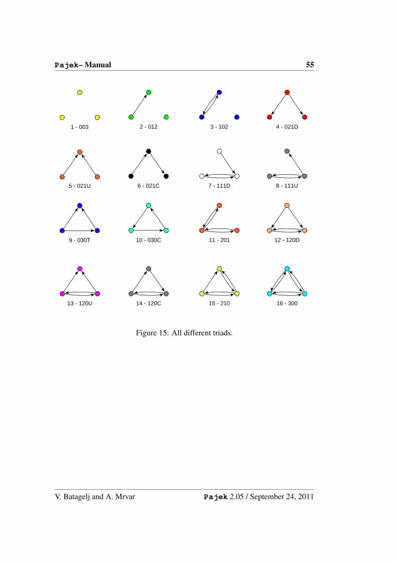
Pajek– Manual 55
1 - 003
2 - 012
3 - 102
4 - 021D
5 - 021U
6 - 021C
7 - 111D
8 - 111U
9 - 030T
10 - 030C
11 - 201
12 - 120D
13 - 120U
14 - 120C
15 - 210
16 - 300
Figure 15: All different triads.
V. Batagelj and A. Mrvar Pajek 2.05 / September 24, 2011

56 Pajek– Draw window
4 Draw Window Tools
4.1 Main Window Draw Tool• Draw - Draw Network. A new window is open, where a new menu appears.
You can edit network by hand (move vertices using left mouse button), se-lect a part of the picture (using right mouse button and select the area), editlines that belong to selected vertex by clicking on vertex using right mousebutton, spin picture using keys X, Y, Z, S, x, y, z, s. Description of Drawwindow menu:
• Draw-Partition – Similar to Draw. Colors of vertices represent the classesin selected partition. Additionally you can put selected vertex or selectedvertices into given class in partition (classes are shown using different col-ors) by clicking on middle mouse button (or Shift+left button) (incrementclass), or together with Alt (or Alt+left button) - decrement class number.In Figure 20 on page 90 you can see which color represents selected class.
Some additional menu items that were already described appeared (you candraw network according to layers from partition and optimise energy usingfixed vertices determined using partition). It is also possible to move theselected class (by clicking close to vertex from that partition).
• Draw-Vector – Sizes of vertices are determined using selected vector.
• Draw-2Vectors – Sizes of vertices are determined using selected two vec-tors (first for width second for height).
• Draw-Partition-Vector – Colors of vertices are determined using selectedpartition, sizes of vertices are determined using selected vector.
• Draw-Partition-2Vectors – Colors of vertices are determined using se-lected partition, sizes of vertices are determined using selected two vectors(first for width second for height).
• Draw-SelectAll – Create null partition and draw network using it.
4.2 LayoutGenerate layout of the network.
• Circular – Position vertices on circle
1. Original – in order determined by the network.
V. Batagelj and A. Mrvar Pajek 2.05 / September 24, 2011

Pajek– Draw window 57
2. using Permutation – in order determined by current permutation.
3. using Partition – create separate circles for clusters in selected par-tition. Center of the circle is determined by the arithmetic mean ofpositions of vertices in the cluster.
4. Random – in random order.
• Energy – Automatic layout generation.
1. Kamada-Kawai – algorithm for automatic layout generation in theplane.
(a) Free – Every position in the plane is possible.(b) Separate Components – Optimize each component separatelly
and tile components at the end.(c) Fix first and last – First and last vertex are fixed in opposite cor-
ners.(d) Fix one vertex in the middle - Select vertex which will be fixed
in the middle of the picture.(e) Selected group only – Only selected part of the picture is taking
into account during optimisation.(f) Fix selected vertices - Selected vertices (from partition) are fixed
on given positions). This item is visible only if Draw partition isactive.
2. Fruchterman Reingold – another algorithm for automatic layoutgeneration (faster than Kamada-Kawai).
(a) 2D – optimisation in plane.(b) 3D – optimisation in space.(c) Factor – Input factor for optimal distance among vertices when
using Fruchterman Reingold optimisation.
3. Starting positions – for energy drawing (random, circular, given po-sitions on plane xy, given z coordinates).
• EigenValues – Drawing using eigenvalues/eigenvectors (Lanczos algorithm).Values of lines can be taken into account or not.
1. 1 1 1 – Select 2 or 3 eigenvalues and algorithm will compute cor-responding eigenvectors. Eigenvalues may be multiple so there aremany possibilities. Some examples
(a) 1 1 1 – compute 3 eigenvectors that correspond to the first eigen-value
V. Batagelj and A. Mrvar Pajek 2.05 / September 24, 2011

58 Pajek– Draw window
Figure 16: VRML display of layout determined by eigenvectors
(b) 1 1 2 – compute 2 eigenvectors that correspond to the first eigen-value and 1 that correspond to the second
(c) 1 2 2 – compute 1 eigenvector that correspond to the first eigen-value and 2 that correspond to the second
(d) 1 2 3 – compute 1 eigenvector that correspond to the first, 1that correspond to the second and 1 that correspond to the thirdeigenvalue
(e) 1 1 – compute 2 eigenvectors that correspond to the first eigen-value (2D picture)
• Tile Components – Tile weakly connected components in a plane.
4.3 LayersVisible only if Draw partition is active. Draw in layers according to partition.
• Type of Layout – Select type of picture (2D – layers in y direction, or 3D– layers in z direction). According to that, appropriate menu appears.
• In y direction – Draw vertices in layers (y coordinate) inside layers drawvertices centered-equidistantly (x coordinate), z coordinate is 0.5 for all ver-tices.
V. Batagelj and A. Mrvar Pajek 2.05 / September 24, 2011

Pajek– Draw window 59
• In y direction+random in x – Same as first option, only vertices are put onlayers in random order not according to vertex numbers.
• In z direction – Draw layers in z direction, live x and y coordinates as theyare.
• In z direction + random in xy – Draw layers in z direction, x and y coor-dinates get random values
• Averaging x coordinate – Use it after vertices are put on layers in 2D.Iterativelly compute average x-coordinate of all neighbors and normalize.Good approximation of global picture, but vertices are put to close to eachother. Use it on all vertices or only on selected one.
• Averaging x and y coordinates – Use it after vertices are put on layers in3D. Iterativelly compute average x and y coordinates of all neighbors andnormalize. Good approximation of global picture, but vertices are put toclose to each other. Use it on all vertices or only on selected one.
• Tile in x direction – After averaging x coordinate vertices are put to close toeach other, so using this option vertices are repositioned to minimal distancedescribed in resolution.
• Tile in xy plane – Same as previous, only this option is used when drawing3D pictures.
• Optimize layers in x direction – Optimize layout in layers using minimiza-tion of the total length of lines.
1. Forward – go from first to last layer. In the current layer optimizeonly layers having numbers equal or one smaller as the current layernumber.
2. Backward – go from last to first layer. In the current layer optimizeonly layers having numbers equal or one larger as the current layernumber.
3. Complete – go from first to last layer. In the current layer optimizeonly layers having numbers equal or one smaller or one larger as thecurrent layer number.
• Optimize layers in xy plane – Same as previous, only this option is usedwhen drawing 3D pictures.
V. Batagelj and A. Mrvar Pajek 2.05 / September 24, 2011

60 Pajek– Draw window
• Resolution – How many additional positions are available on layers. Worksonly if Pgraph is selected. The higher the resolution, the better is the resultof optimization, but also slower.
4.4 GraphOnlyShow complete picture without labels and arrows.
4.5 PreviousDraw previous network, and/or partition and/or vector which are loaded in Pajek(depending on selection in Options/PreviousNext/Apply to).
4.6 RedrawRedraw network.
4.7 NextDraw next network, and/or partition and/or vector which are loaded in Pajek(depending on selection in Options/ PreviousNext/ Apply to).
4.8 ZoomOutZoom out (visible only when zooming in layout).
4.9 OptionsAdditional options for picture layout.
• Transform – Transformations of picture.
1. Fit area
(a) max(x), max(y), max(z) – Draw picture as big as possible to fitarea (resize each coordinate to fit in picture independently).
(b) max(x,y,z) – Resize to fit in area but keep real proportions (re-size according to largest distance in all three coordinates, e.g.molecule).
2. Resize – Resize picture (or selected part of it) in all three directionsfor selected factor.
V. Batagelj and A. Mrvar Pajek 2.05 / September 24, 2011

Pajek– Draw window 61
3. Translate – Translate picture (or selected part of it) in space.
4. Reflect y axis – Reflect picture (or selected part of it) around y axis.
5. Rotate 2D – Rotate picture (or selected part of it) in xy plane.
6. Fisheye – Fisheye transformation (cartesian or polar) of picture. If novertex is selected the middle point of picture (or selected part of it) isused as focus, otherwise first selected vertex will be used as focus.
• Values of lines – Meaning of values of lines during energy drawing oreigenvectors computing (no meaning, similarities, dissimilarities (distances)).
• Mark vertices using – Labels can be marked using
1. labels
2. numbers
3. partition clusters (if partition of the same size is also selected)
4. vector values (if vector of the same size is also selected)
5. without labels
6. without labels and arrows
7. cluster only – only vertices belonging to the current Cluster are labeledin the layout.
• Lines – Select the way the lines are drawn:
1. Draw Lines
(a) Edges – draw edges or not(b) Arcs – draw arcs or not(c) Relations – draw all lines (leave empty string) or just lines be-
longing to selected relations, e.g. 1-3,6,10-15.
2. Mark Lines
(a) No – do not mark lines(b) with Labels(c) with Values
3. Different Widths – if checked, the width of the lines will be deter-mined by their line values.
4. GreyScale – if checked, the color in grayscale of lines will be deter-mined by their line values.
V. Batagelj and A. Mrvar Pajek 2.05 / September 24, 2011

62 Pajek– Draw window
• Size – Determine size of vertices, width of vertices border, width of lines,size of arrows, size of font or turn them to default values.Sizes of vertices can be set to autosize (0-average). They can be read frominput file (x fact and y fact) or determined by one vector (currently selected)or the two currently selected vectors. FontSize can be proportional to valuesstored in third partition.
• Colors – Determine color of background, vertices, border of vertices, edges,arcs and font (of vertices labels and lines labels) or turn them to defaultvalues. Colors of edges/arcs can represent relation number of lines. Youcan select which color should represent given class using Relation Col-ors. You can also use colors of vertices (ic Red), border of vertices (bcBlue), arcs and edges (c Green) as defined on input file (see Figure 19,page 89). FontColor can be determined by values stored in second partition.Additionally to predefined colors it is possible to specify colors using RGB(e.g. RGBFF0000, or RGB(1,0,0)) and CMYK (e.g. CMYK00FF0000,or CMYK(0,1,0,0)) format. Note that there should be no spaces in stringdefining a color.Example NET file:
*Vertices 91 "a" ic Pink bc Black2 "b" ic CMYK(0,0,1,0.0) bc CMYKFF0000003 "c" ic Cyan bc Yellow4 "d" ic Purple bc Orange5 "e" ic Orange bc Brown6 "f" ic Magenta bc Green7 "g" ic Brown bc Magenta8 "h" ic RGB(1,0,0) bc Blue9 "i" ic Green bc Magenta
*Arcs1 2 1 c RGB0000FF2 3 1 c Red3 4 1 c Black4 5 1 c Yellow5 6 1 c Gray6 7 1 c Cyan7 8 1 c Magenta8 9 1 c Purple9 1 1 c Brown
• Layout – Layout options
1. Redraw – Redraw whole network during or/and after moving of se-lected vertex, and/or redraw if draw window is paint.
2. Real xy proportions – The draw window has always square shape ornot.
V. Batagelj and A. Mrvar Pajek 2.05 / September 24, 2011

Pajek– Draw window 63
3. Arrows in the Middle – Draw arrows in the middle of lines – not atterminal vertices.
4. Size of vertex 0 – How to handle vertices of size 0 (size of vertex isdetermined in input file or using vector)?
(a) Hide vertex – vertices of size 0 are shown or not.(b) Hide attached lines – lines with one end in vertex of size 0 are
shown or not.
5. Decimal Places – How many decimal places to use when markingvertices using vectors.
6. Show SubLabel – Select the position of the vertices sublabel that isshown in network layouts.
• ScrollBar On/Off – Show/Hide the scrollbars in the top left corner of Drawwindow. When part of picture is selected, scrollbar is used for moving.When whole picture is selected, scrollbar is used for spinning (like pressingkeys X, Y, Z, x, y, z – spinning around axis defined by the key, and S – spinaround selected normal)
• Interrupt – Interrupt period during optimisation (stop every ? second, ornot)
• Previous/Next – Select parameters when using Previous or Next commandsfor drawing sequence of networks in draw window:
1. Max. number – How many networks to show in sequence. If thenumber is higher than number of existing networks the sequence willstop earlier.
2. Seconds to wait – Seconds to wait between the two layouts.
3. Optimize Layouts – Optimize the current layout or not. If the se-quence of networks is obtained from the same network, it is useful tochoose Energy/Starting Positions/ Given xy to start optimization withexisting coordinates.
(a) Kamada-Kawai – Optimize the current layout usingKamada-Kawai algorithm.
(b) 2D Frucht. Rein. – Optimize the current layout using 2D Frucht.Rein. algorithm.
(c) 3D Frucht. Rein. – Optimize the current layout using 3D Frucht.Rein. algorithm.
(d) No – Do not optimize the layout, just show the picture.
V. Batagelj and A. Mrvar Pajek 2.05 / September 24, 2011

64 Pajek– Draw window
4. Apply to – Which object (Network, Partition, Vector) will changewhen Previous or Next is selected:
(a) Network – The previous / next network in memory is drawn. IfDraw-Partition is selected and the new network matches in di-mension with selected partition, the same partition will determinecolors of vertices of the new network. If Draw-Vector is selectedand the new network matches in dimension with selected vector,the same vector will determine sizes of vertices of the new net-work.Option can be used to show several networks of equal size usingthe same partition/vector.
(b) Partition – The previous / next partition in memory is selected. IfDraw-Partition is selected: The same network is drawn using pre-vious / next partition (network and partition must match in size).Option can be used to show several partitions of selected network.
(c) Vector – The previous / next vector in memory is selected. IfDraw-Vector is selected: The same network is drawn using previ-ous / next vector (network and vector must match in size).Option can be used to show several vectors of selected network.
By checking several objects (Network, Partition, Vector) at the sametime previous / next networks will be drawn using previous / next parti-tions and (or) vectors at the same time. All consequent selected objectsmust match in size.
• Select all – Select all vertices in window (then possible to put vertices ingiven class).
4.10 Export
Export layout of the network to one of the following two or three dimensionalformats:
• 2D – two dimensional exports:
– EPS/PS – Export to EPS format (with or without Clip, or WYSIWYG[What You See Is What You Get – exported EPS picture is similar topicture in Draw window – except that colors are Black/White or colordetermined by partition]). PS – Export to PS format (similar to EPSbut without header).
V. Batagelj and A. Mrvar Pajek 2.05 / September 24, 2011

Pajek– Draw window 65
– SVG – Export to SVG (Scalable Vector Graphics) format. Additionalcontrols over layout can be included in SVG or HTML. The plugin forexamining layouts can be obtained from Adobe [1].Linear or radial gradients (continuously smooth color transitions fromone color to another) can be selected as well – up to three backgroundcolors can be selected in Export/Options window.
1. General – Export to SVG without possibility to choose parts ofthe picture.
2. Labels/Arcs/Edges – Export with possibility to turn labels, arcsand/or edges on/off.
3. Partition – Export to SVG using one or two partitions. One parti-tion is used by default: the same partition determines classes andcolors. But, if two partitions are defined by Partitions menu, firstpartition will determine classes, the second colors of vertices.(a) Classes – User can turn selected classes and lines among
classes on/off.(b) Classes with semi-lines – User can turn selected classes on/off.
Lines among classes are drawn as semi-lines.(c) Nested Classes – Upper classes are nested in lower – when-
ever selected class is turned on all higher classes are turned ontoo, and all lower classes are turned off (suitable for showingcores, for example).
4. Line Values – Export to SVG using values of lines. Thresholdvalues or number of classes must be given. If you input #n, nclasses of equal size will be generated. According to obtainedthresholds, subsets of lines (and incident vertices) are defined andcan be turned on/off inside web browser.(a) Classes – User can turn lines of selected value and incident
vertices on/off.(b) Nested classes – User can turn lines of selected value or
higher (lower) and incident vertices on (off).(c) Options – Additional options to emphasize the values of lines
using some visual properties.Different Colors – Subsets of lines are drawn using colorswhich are used for partitioning vertices too.Using GreyScale – The darkness of a line corresponds to itsvalue.Different Widths – The width of a line corresponds to itsvalue.
V. Batagelj and A. Mrvar Pajek 2.05 / September 24, 2011

66 Pajek– Draw window
5. Multiple Relations Network – Export multiple relations networkto SVG. User can show/hide one or more relations in the layout.
6. Current and all Subsequent – If checked the current networkand all subsequent networks will be exported to SVG. For eachnetwork separate html file is generated. Files are given the fol-lowing names: file001.htm, file002.htm,... Generated html filesget additional links (Previous/Next) to transition among them. Ifalso next partitions / vectors fit in dimension to dimension of net-works, partitions will determine color of vertices, vectors will de-termine sizes of vertices. Subsequent is applied to any combina-tion of [Network, Partition, Vector] (one of the three objects only,any pair of them or all three of them) according to selection inOptions/Previous/Next/ Apply to in Draw window.
– Bitmap – Export to Windows bitmap (bmp) format.
• 3D – three dimensional exports:
– X3D – Export to X3D (XML based 3D computer graphics, the suc-cessor of VRML) format.
– Kinemages – Export to Kinemages format with balls or labels. Youneed Mage or King viewer to watch it. A free copy of the Mage soft-ware can be downloaded from its site [58].
1. Current Network Only – Export only current network to Kine-mages. Two partitions defined by Partitions menu can be used -one for generations one for colors.
2. Current and all Subsequent – Export current network and allsubsequent networks (use commands KINEMAGE/Next or CtrlN in Mage). If also next partitions/vectors fit in dimension to di-mension of networks, partitions will determine color of vertices,vectors will determine sizes of vertices. Subsequent is applied toany combination of [Network, Partition, Vector] (one of the threeobjects only, any pair of them or all three of them) according toselection in Options/Previous/Next/ Apply to in Draw window.
3. Multiple Relations Network – Export with possibility to hide /show selected relations.
– VRML – Export to VRML (Virtual Reality) format. For examiningit you need a VRML viewer such as Cortona [29] or (older) Cosmoplayer [30].
V. Batagelj and A. Mrvar Pajek 2.05 / September 24, 2011

Pajek– Draw window 67
– MDL MOL file – Export to MDL Molfile format. You need Chimeplugin (Chemscape Chime) for Netscape to explore it [51].
• Options – EPS, SVG, X3D and VRML default options (see section on Ex-ports to EPS/SVG/X3D/VRML).
• Append to Pajek project file – Add current network to the end of selectedproject file (used by program PajekToSvgAnim).
– Select file – Select project file.
– Append – Append to project file.
4.11 Spin• Spin around – Spin network around selected normal.
• Perspective – Distant vertices are drawn smaller (or not).
• Normal – Normal vector to spin around.
• Step in degrees – Step in degrees when showing rotation.
4.12 MoveGive additional constraints on hand vertex moving:
• Fix – Fix (do not allow) moving in x or y direction, or do not allow changingdistance from center (circulating).
• Grid – Define (x, y) positions on grid, these become feasible positions forvertices during moving by hand.
• Circle – Define (x, y) positions on concentric circles, these become feasiblepositions for vertices during moving by hand.
• Grasp – Determine which additional vertices are moving when clickingwith left mouse button close to vertex in given class. Vertices that will bemoved are in the:
1. Closest Class Only
2. Closest Class and Higher
3. Closest Class and Lower
V. Batagelj and A. Mrvar Pajek 2.05 / September 24, 2011

68 Pajek– Draw window
4.13 Info– Select aesthetic properties of the current layout to compute:
• Closest Vertices
• Smallest Angle
• Shortest/Longest Line
• Number of crossings if lines
• Vertex Closest to Line
• All Properties
Remember that coordinates of vertices must be between 0 and 1!
V. Batagelj and A. Mrvar Pajek 2.05 / September 24, 2011

Exports to EPS/SVG/X3D/VRML 69
5 Exports to EPS/SVG/X3D/VRML
5.1 DefaultsIf you have no labels in Draw window when you call Export there will also be nolabels in EPS/SVG picture, otherwise numbers/labels like in Draw window willbe shown. If you are looking at the picture using Draw/Partition, the same colorswill be automatically used in EPS/SVG picture too.
5.2 Parameters in EPS, SVG, X3D, and VRML Defaults Win-dow
Window is divided into 5 frames, two on the left and three on the right.Note that settings you made in this window are overwritten if the parameters
are specified in Pajek input (NET) file.
Top frame on the left – EPS/SVG Vertex Default
This frame defines default drawing of vertices when we export layouts to EPS andSVG:
• Interior Color – interior color of vertices (see Figure 19, page 89). Ifdrawing using Partition is used, partition colors will overwrite the specifiedinterior color.
• Border Color – color of the borderline of vertices.
• Label Color – color of label of vertices.
• Border Width – width of the borderline of vertices.
• Label Position: Radius /Angle – position where the label will be dis-played:
– Radius – distance of beginning of vertex label from vertex center –first polar parameter.
– Angle – position of vertex label in degrees - second polar parameter(0..360).
If radius is equal to 0, the label will be centered, otherwise it will be leftaligned on the specified position.
• Fontsize – size of font of vertices labels.
V. Batagelj and A. Mrvar Pajek 2.05 / September 24, 2011

70 Exports to EPS/SVG/X3D/VRML
• Label Angle – angle in which vertex labels will be displayed: if angle issmaller than 360, it means relative according to horizontal line (0 – horizon-tally); otherwise it is relative to center of the layout (360 – concentrically).The latter is useful when all vertices are drawn in concentric circle(s) usingLayout/Circular.
• x/y Ratio – ratio between size of vertex in x and y direction (e.g., value 1for circle, value larger/smaller than 1 for ellipse).
• Shape – default shape of vertex (ellipse, box, or diamond).
• Shapes file – default shapes file, double click to change it.
• Export options overwrite shapes file – if checked: options selected in thiswindow overwrite options defined in shapes file, otherwise default valuesfor each shape are defined in selected shapes file.
Bottom frame on the left – EPS/SVG Line Default
This frame defines default drawing of lines when we export layouts to EPS andSVG:
• Edge Color – color of edges.
• Edge Width – width of edges.
• Arc Color – color of arcs.
• Arc Width – width of arcs.
• Pattern – pattern for drawing lines (Solid or Dots).
• Arrow Size – size of arrows.
• Arrow Position – distance of arrow from terminal vertex: If distance isbetween 0 and 1, it means relative distance according to arc length, e.g.: 0 –arrow touching the terminal vertex; 0.5 – arrow in the middle of the arc. Ifdistance is larger than 1 it means absolute distance from the terminal vertex(this is useful if you want to have all arcs on the same distance from terminalvertex, regardless of arcs length)
• Label Color – color of line labels.
• Label Angle – angle in which label of line will be displayed: if angle issmaller than 360, it means relative to direction of line (0 – parallel to line);otherwise it is relative to horizontal line (360 – horizontally).
V. Batagelj and A. Mrvar Pajek 2.05 / September 24, 2011

Exports to EPS/SVG/X3D/VRML 71
• Label Position – position of the center of line label – position is point onthe line - distance of the center of line label from terminal vertex (see alsoArrow Position)
• Fontsize – size of font of line labels.
• Label Position: Radius /Angle – position where the center of line labelwill be displayed according (relative) to Label Position:
– Radius – distance of center of line label from point defined by LabelPosition - first polar parameter.
– Angle – position of label in degrees - second polar parameter (0..360).
• Only straight lines – drawing bidireced and multiple lines without curves.
Top frame on the right
This frame defines some additional defaults when we export layouts to EPS, SVG,X3D, or VRML:
• EPS, SVG, X3D, VRML Size of Vertices – default size of vertices whenexporting to X3D/VRML (valid for EPS and SVG exports as well).
• X3D/VRML Size of Lines – width of lines in X3D/VRML.
• EPS: Use RGB colors instead of CMYK – in description of colors in EPSfile RGB is used (default is CMYK).
• SVG: 3D Effect on Vertices – if selected, gradient will be applied to get3D look of vertices.
Middle frame on the right – Background Colors
This frame defines background color when exporting to EPS/SVG/X3D/VRMLand gradients (continuously smooth color transitions from one color to another)when exporting layouts to SVG/X3D:
• Bckg. Color 1 – Background color for layout in EPS/SVG/X3D/VRML.
• Bckg. Color 2 – the second color for SVG/X3D export. No – means withoutsecond color, otherwise selected gradient will be used.
• Bckg. Color 3 – the third color for SVG/X3D export – gradient.
• Gradients – type of gradient to use in SVG (No, Linear, or Radial). In X3Donly Radial gradient is supported.
V. Batagelj and A. Mrvar Pajek 2.05 / September 24, 2011

72 Exports to EPS/SVG/X3D/VRML
Bottom frame on the right
This frame defines some additional defaults when we export layouts to EPS:
• Left, Right, Top, Bottom – additional border around layout when exportingto EPS (only when EPS Clip format is selected)
• Border Color – color of borderline of layout. It is used for export to SVGas well. No – means without borderline.
• Border Radius – radius of borderline of layout (if greater than 0 it meansoval instead of rectangle).
• Border Width – width of borderline of layout.
Figure 17: Spider / Krizevec; Photo: Stana.
V. Batagelj and A. Mrvar Pajek 2.05 / September 24, 2011

Exports to EPS/SVG/X3D/VRML 73
5.3 Exporting pictures to EPS/SVG – defining parameters ininput file
Definition of Network (and its picture) on Input ASCII File
For every vertex and line we can specify in details how it should be drawn (colors,shapes, sizes, patterns, rotations, widths...).
A kind of standardized language is used for describing networks. The follow-ing reserved words are used:
1. *Vertices n – definition of vertices follows. n is number of vertices. Eachvertex is described using following description line:
vertex num label [x y z] [shape] [changes of default parameters]
Explanation:
• vertex num – vertex number (1, 2, 3 . . . n)
• label – if label starts with character A..Z or 0..9 first blank determinesend of the label (e.g., vertex1), labels consisting of more words mustbe enclosed in pair of special characters (e.g., ”vertex 1”)
• x, y, z – coordinates of vertex (between 0 and 1)
• shape – shape of object which represents vertex. Shapes are definedin file SHAPES.CFG (ellipse, box, diamond, triangle, cross, empty)Description of parameters in shapes.cfg:
– SHAPE s – s is external name of vertex (used in Pajek networkfile)
– sh – sh can be ellipse, box, diamond, triangle, cross, empty. Thisis the name of PostScript procedure that actually draws object(procedure is defined in drawnet.pro).
– s size – default size– x fact – magnification in x direction– y fact – magnification in y direction– phi – rotation in degrees of object in + direction (0..360)– r – parameter used for rectangle and diamond for describing ra-
dius of corners (r = 0 – rectangle, r > 0 – roundangle)– q – parameter used for diamonds – ratio between top and middle
side of diamond (try q 0.01, q 0.5, q 2, ...)– ic – interior color of vertex. See Figure 19, page 89 for the list of
possible colors.– bc – boundary color of vertex
V. Batagelj and A. Mrvar Pajek 2.05 / September 24, 2011

74 Exports to EPS/SVG/X3D/VRML
– bw – boundary width of vertex– lc – label color– la – label angle in degrees (0..360)– lr – distance of beginning of vertex label from vertex center (ra-
dius – first polar parameter)– lphi – position of label in degrees (0..360) (angle phi – second
polar parameter)– fos – font size– font – PostScript font used for writing labels (Helvetica, Courier,
...)– HOOKS – positions where edges can join the selected shape - ac-
cording to s size. Three different ways to specify these positions:(a) CART – x y – positions in Cartesian coordinates (x,y)(b) POLAR – r phi – positions in polar coordinates, phi is posi-
tive angle (0..360)(c) CIRC – r phi1 – iteration of positions in polar coordinates r
– radius, phi = k ∗ phi1, k = 1, 2, ..; k ∗ phi1 ≤ 360
Default values can be changed for each vertex in definition line, example:1 ”vertex one” 0.3456 0.1234 0.5 box ic White fos 20
Explanation: White box will represent vertex 1, label (vertex one) will bedisplayed using font size 20.
2. *Arcs (or *Edges) – definition of arcs (edges). Format:
v1 v2 value [additional parameters]
Explanation:
• v1 – initial vertex number
• v2 – terminal vertex number
• value – value of arc from v1 to v2
These three parameters must always be present. If no other parameter isspecified, the default arc will be black, straight, solid arc with followingexceptions:
• if value is negative, dotted line will be used instead of solid,
• if arc is a loop (arc to itself) bezier loop will be drawn,
• if bidirected arc exists two curved bezier arcs will be drawn.
V. Batagelj and A. Mrvar Pajek 2.05 / September 24, 2011

Exports to EPS/SVG/X3D/VRML 75
Arrow will be drawn at the end of the edge (at terminal vertex).
As we mentioned, hooks are used to specify exact position where line joinsvertices.
Additional parameters:
• w – width of line
• c – color of line
• p – pattern of line (Solid, Dots)
• s – size of arrow
• a – type (shape) of arrow (A or B)
• ap – position of arrow
– ap = 0 – arrow at terminal vertex– 0 < ap ≤ 1 – proportional distance from terminal vertex (accord-
ing to line length)– ap > 1 – absolute distance
• l – line label (e.g. ”line 1 2”)
• lp – label position (look at ap)
• lr – label radius (position of center text from point on edge )
• lphi – label radius (angle of center text according to point on edge ) (lrand lphi are polar coordinates)
• lc – label color
• la – label angle(0 < la < 360 – relative to edge, la ≥ 360 – absolute angle accordingto x axis)
• fos – font size of label
• font – PostScript font used for writing labels (Helvetica, Courier, ...)
• h1 – hook at initial vertex (0 – center, -1 the closest, 1, 2.. user defined)
• h2 – hook at terminal vertex
• a1 – angle at initial vertex (Bezier)
• k1 – velocity at initial vertex (Bezier)
• k2 – velocity at terminal vertex (Bezier)
• a2 – angle at terminal vertex (Bezier)
V. Batagelj and A. Mrvar Pajek 2.05 / September 24, 2011
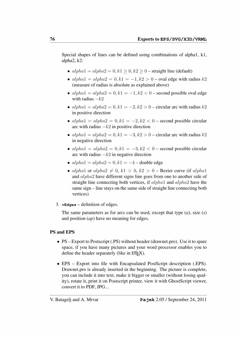
76 Exports to EPS/SVG/X3D/VRML
Special shapes of lines can be defined using combinations of alpha1, k1,alpha2, k2:
• alpha1 = alpha2 = 0, k1 ≥ 0, k2 ≥ 0 – straight line (default)
• alpha1 = alpha2 = 0, k1 = −1, k2 > 0 – oval edge with radius k2(measure of radius is absolute as explained above)
• alpha1 = alpha2 = 0, k1 = −1, k2 < 0 – second possible oval edgewith radius −k2• alpha1 = alpha2 = 0, k1 = −2, k2 > 0 – circular arc with radius k2
in positive direction
• alpha1 = alpha2 = 0, k1 = −2, k2 < 0 – second possible circulararc with radius −k2 in positive direction
• alpha1 = alpha2 = 0, k1 = −3, k2 > 0 – circular arc with radius k2in negative direction
• alpha1 = alpha2 = 0, k1 = −3, k2 < 0 – second possible circulararc with radius −k2 in negative direction
• alpha1 = alpha2 = 0, k1 = −4 – double edge
• alpha1 or alpha2 6= 0, k1 > 0, k2 > 0 – Bezier curve (if alpha1and alpha2 have different signs line goes from one to another side ofstraight line connecting both vertices, if alpha1 and alpha2 have thesame sign – line stays on the same side of straight line connecting bothvertices)
3. *Edges – definition of edges.
The same parameters as for arcs can be used, except that type (a), size (s)and position (ap) have no meaning for edges.
PS and EPS
• PS – Export to Postscript (.PS) without header (drawnet.pro). Use it to sparespace, if you have many pictures and your word processor enables you todefine the header separately (like in LATEX).
• EPS – Export into file with Encapsulated PostScript description (.EPS).Drawnet.pro is already inserted in the beginning. The picture is complete,you can include it into text, make it bigger or smaller (without losing qual-ity), rotate it, print it on Postscript printer, view it with GhostScript viewer,convert it to PDF, JPG...
V. Batagelj and A. Mrvar Pajek 2.05 / September 24, 2011

Exports to EPS/SVG/X3D/VRML 77
An example*Vertices 41 "ellipse" 0.120 0.285 0.5 ellipse x_fact 5 y_fact 3 fos 20 ic LightYellow lc Red2 "box" 0.818 0.246 0.5 box x_fact 5 y_fact 3 fos 20 ic LightCyan lc Blue3 "diamond" 0.368 0.779 0.5 diamond x_fact 7 y_fact 3 fos 20 ic LightGreen lc Black4 "triangle" 0.835 0.833 0.5 triangle x_fact 9 y_fact 3 fos 20 ic LightOrange lc Brown lr 30 lphi 200*Arcs1 1 1 h2 0 w 3 c Blue s 2 a1 -130 k1 0.6 a2 -130 k2 0.6 ap 0.25 l "Bezier loop" lc OliveGreen fos 20 lr 13 lp 0.5 la 3602 1 1 h2 1 a1 120 k1 1 a2 10 k2 0.8 ap 0 l "Bezier arc" lphi 270 la 180 lr 13 lp 0.51 2 1 h2 -1 a1 40 k1 2 a2 -30 k2 0.8 ap 0 l "Bezier arc" lphi 90 la 0 lp 0.754 2 -1 l "Straight dotted arc" p Dots c Red*Edges1 3 1 l "Straight edge" lp 0.43 4 1 l "Straight edge"
You have to set some options in Pajek’s draw window: for exampleOptions / Lines / Mark Lines / with labels
to activate the display of line labels.
Bezier loopBezier arc
Bezier arcS
trai
ght d
otte
d ar
c
Straight edge
Straight edge
ellipsebox
diamond
triangle
Figure 18: Example picture
5.4 Using Unicode in Pajek’s picturesSometimes we would like to use in Pajek’s picture some characters from unusualalphabets (special symbols, Cyrillic, Greek, Arabic, Chinese, ...). They are avail-able in Unicode. Pajek supports Unicode UTF8 files with BOM from version 2.00on.
V. Batagelj and A. Mrvar Pajek 2.05 / September 24, 2011

78 Exports to EPS/SVG/X3D/VRML
Some hints on using Unicode in Pajek:
• Using the free Unicode editor BabelPad we prepare the Unicode versionof the *.NET file. Use the U tool (Unicode table) to enter the Unicodecharacters.
• Using the BabelPad option File/Save as/UTF8 and checking ByteOrder Mark you save network in a Unicode file.You can use also File/Save as/ASCII plus decimal NCR. Inthis way we transform Unicode file into an ASCII file in which the Uni-code characters are represented using numeric codes &#dddd;.
Any of the two files generated can be read by Pajek and proper Unicodecharacters will appear in Draw, Report and other windows provided that youselect proper proportional and monospaced font in Options/SelectFont in Pajek Main menu. We suggest to use Arial Unicode MS orLucida Sans Unicode (one of them usually comes with Windows) forproportional font and GNU Unifont for monospaced font. Courier Newcan be used too.
When saving networks they are stored as ASCII files by default (nonASCIIcharacters are stored as &#dddd;) unless you check Options/Read-Write/SaveFiles as Unicode UTF8 with BOM.
The file is used in Pajek 2.00 (or higher) to produce picture. The picture isexported in the SVG format.
Pajek
Vlado
Андреј
צעשהגלז
يريخبتصك
गङथफञऑक
∰∈∀≋∞⊚
⑤⑨④②⑦
♔♕♖♗♘♙
焹焓燝牕犫獨
ανδρει
Pajek
Vlado
Андреј
צעשהגלז
يريخبتصك
गङथफञऑक
∰∈∀≋∞⊚
⑤⑨④②⑦
♔♕♖♗♘♙
焹焓燝牕犫獨
ανδρει
• The SVG picture can be opened in the free drawing program InkScape.Here we can make some additional enhancements of the picture.
V. Batagelj and A. Mrvar Pajek 2.05 / September 24, 2011

Exports to EPS/SVG/X3D/VRML 79
• In InkScape we can, using the option File/Save as/pdf or eps, savethe picture in the desired format PDF or EPS or some other) with labels con-taining Unicode characters. Note that the PDF (1.4 or higher) also supportsthe transparency. The EPS file can be inserted in Word document.
A set of example files is available in ZIP.Similar approach can be used also for 3D models in X3D. For their inspection
we recommend the use of Instant Player.
V. Batagelj and A. Mrvar Pajek 2.05 / September 24, 2011

80 Using Macros in Pajek
6 Using Macros in Pajek
6.1 What is a Macro?A macro enables you to record a sequence of primitive Pajek commands into afile. You can use this file later to execute the saved sequence of commands withoutselecting one by one.
6.2 How to record a Macro?1. First load all objects (networks, partitions,...) which will be used by a
macro.
2. Select objects which will be used in macro (for example, network whichwill be first used must be shown in Network ComboBox).
3. Choose Macro/Record and select the name of macro file (default extensionis .mcr).
4. Use Pajek as usual to define a sequence of commands. We advise toadd additional comments to macro file using Macro/Add Message. Whenrunning macro this comments are displayed in Report window and help youto follow the macro execution.
5. At the end select Macro/Record again to stop recording.
6.3 How to execute the Macro?1. First load object(s) that will be used as input in macro execution.
2. Choose Macro/Play and select the macro file.
6.4 ExampleThe following macro performs topological sort of an acyclic network:
NETBEGIN 2CLUBEGIN 1PERBEGIN 1CLSBEGIN 1HIEBEGIN 1VECBEGIN 1NETPARAM 1
V. Batagelj and A. Mrvar Pajek 2.05 / September 24, 2011

Using Macros in Pajek 81
Msg Depth PartitionC 1 DEP 1 (10)Msg Make PermutationP 1 MPER 1 (10)Msg Reordering networkN 2 REOR 1 1 (10)
The first seven commands store the current state of ComboBoxes. The acyclicnetwork on which we want to execute topological sort must be at the top of Net-work ComboBox before starting the macro.
6.5 List of macros available in installation file6.5.1 Macros prepared for genealogies and other acyclic networks
• Path – find shortest chain (undirected path) between the two vertices.
• Descendants – find all vertices ’later’ than selected vertex (in a p-graph).
• Ancestors – find all vertices ’before’ the selected vertex (in a p-graph).
• Cognatic3 – find vertices three generations ’before’ and three generations’after’ the selected vertex (in a p-graph).
• Cognatic – find all reachable vertices ’before’ and all ’after’ the selectedvertex (in a p-graph).
• Layers, Layers1, Layers2 – draw acyclic network in layers (different al-gorithms).
• zLayers – draw acyclic network in layers in z direction.
• LongestPatrilineage – find the longest patrilineage in Ore-genealogy. Thegenealogy must be read with the option Ore graph: 1-Male, 2-Female
links checked.
• LongestMatrilineage – find the longest matrilineage in Ore-genealogy. Thegenealogy must be read with the option Ore graph: 1-Male, 2-Female
links checked.
• NumDescendants – for each vertex compute the size of output domain(number of descendants in Ore-graph).
• NumAncestors – for each vertex compute the size of input domain (numberof ancestors in Ore-graph).
V. Batagelj and A. Mrvar Pajek 2.05 / September 24, 2011

82 Using Macros in Pajek
6.5.2 Macros prepared for computing derived kinship relations
Pajek generates three relations when reading genealogy as Ore graph with theoption Ore graph: 1-Male, 2-Female links checked:
1 : is a father of2 : is a mother of3 : is a spouse of
Other kinship relations can be obtained from these relations by running macros.Gender partition is also result of reading genealogy and is input to the followingmacros.
4 : is a parent of5 : is a child of6 : is a son of7 : is a daughter of8 : is a husband of9 : is a wife of
10 : is a sibling of11 : is a brother of12 : is a sister of13 : is an uncle of14 : is an aunt of15 : is a semisibling of
Using macro add all relations you can add all above relations at once.As a test/example file you can use */pajek/data/family.ged
6.6 Repeating last commandMacro submenu enables to run the last command executed by Pajek several timesapplied to different successive objects, as well.
Example: after loading 100 networks in Pajek, execute degree partition onthe first network and run Repeat Last Command by typing 99 to compute degreepartition on all other networks.
Commands that include several objects can be run as well (e.g. extracting sub-networks according to selected partition(s)). There are 3 different possibilities forextracting from the set of networks (possibilities are selected by fixing appropriateobjects):
• for all networks extracting is determined by the same partition (increment-ing applied to network, not applied to partition – partition is fixed)
V. Batagelj and A. Mrvar Pajek 2.05 / September 24, 2011

Using Macros in Pajek 83
• for all networks extracting is determined by another partition (incrementingapplied to network and to partition – nothing is fixed)
• for one network several extractions are determined by different partitions(incrementing not applied to network, applied to partition – network isfixed)
Important: Always first execute the command on the first loaded object(s).Repeating will start with object(s) that have object number(s) one higher than theobject(s) on which the command was executed.
If the result of the command is also a constant, all constants are stored in avector. In Pajek the following constants exist: number of vertices, arcs, edges,network densities, centralization indices, diameter, relinking index, correlationand contingency coefficients, number of fragments, main core number, numberof components, length of critical path, maximum flow, distance between vertices,number of islands, minimum and maximum value in partition / hierarchy, mini-mum, maximum, arithmetic mean, median and standard deviation in vector.
V. Batagelj and A. Mrvar Pajek 2.05 / September 24, 2011

84 Blockmodeling in Pajek
7 Blockmodeling in PajekThe blockmodeling option is an embedding of the programs for optimization ap-proach to generalized blockmodeling MODEL2 and TwoMODEL from packageSTRAN – STRucture ANalysis [9] into Pajek.
The blockmodeling command seeks for the best partition of a given networksatisfying given types of blocks – generalized blockmodeling [7, 35]. The block-model can be built inside Pajek (if User Defined is selected) and/or its descriptioncan be stored in MDL file. The impact of errors in each block can be controlledusing penalty weights.
The option supports also generalized blockmodeling of two-mode networks[34].
The maximum size of a network on which the command can be applied is 250vertices. But the real limit is time complexity – already on 100 vertices optimiza-tion can last some hours.
The results of the command are stored as partitions. They can be displayed asa picture
Draw / Draw-PartitionandLayout / Energy / Kamada-Kawai / FreeorLayout / Circular / using Partition
The result can be displayed also in the matrix form. This requires two steps:Partition / Make PermutationFile / Network / Export Matrix to EPS /
Using Permutation enter file name; yes
7.1 MDL filesThe structure of a MDL file is evident from the following example
*MODEL Tina90 3 100 0 1 2 3 4
*CONSTRAINTS1 100 2 14 100 1 3
*EOM
The first character in each line should be a star * or a blank.The last character in a line should not be a blank.
V. Batagelj and A. Mrvar Pajek 2.05 / September 24, 2011

Blockmodeling in Pajek 85
A number in the second line is number of clusters. In the case of two-modenetwork two numbers should be given in this line – number of row-clusters andnumber of col-clusters. The other data are the same for both type of networks.The following lines have the structure
i j penalty t1 t2 . . . tk
When i, j > 0 the line prescribes that the block (i, j) can be of types t1, t2 . . . tk.The types are coded as follows
0 - - null 7 rfn - row-function1 com - complete 8 cfn - col-function2 rdo - row-dominant 9 den - density3 cdo - col-dominant 10 dnc - do not care4 reg - regular 11 one - non-null5 rre - row-regular 12 sym - symmetric6 cre - col-regular
Lines with i = 0 defines the types of of parts of model matrix:
• j = 0: diagonal (for one-mode networks only);
• j = 1: upper triangle (for one-mode networks only);
• j = 2: lower triangle (for one-mode networks only);
• j = 3: complete matrix.
In the case of several lines describing the same block the last prescriptionprevails.
Lines following *CONSTRAINTS define additional constraints in blockmodel.Constraints have the form
k penalty i j
with the following meaning
• k = 1: i ∈ Cj – vertex i belongs to cluster Cj;
• k = 2: i /∈ Cj – vertex i does not belong to cluster Cj;
• k = 3: C(i) = C(j) – vertices i and j belong to the same cluster;
• k = 4: C(i) 6= C(j) – vertices i and j belong to different clusters;
• k = 5: i ≤ |C(j)| – cluster Cj contains at least i vertices;
V. Batagelj and A. Mrvar Pajek 2.05 / September 24, 2011

86 Blockmodeling in Pajek
• k = 6: i ≥ |C(j)| – cluster Cj contains at most i vertices.
Be careful in the case of two mode network for constraints of type k = 5 andk = 6 (constraints on min/max number of vertices in selected cluster): If thereare r row-clusters and c col-clusters in blockmodel, then use numbers in the range1 . . . r to define constraint on row-cluster and numbers in the range r+ 1 . . . r+ cto define constraint on col-cluster.
The violations of constraints contribute to criterion function with a term
+ # of violations × penalty
The values of penalties have to be in the range 0 to 1000.
7.2 Examples of MDL files7.2.1 Regular blocks
*MODEL Regular100 3 1 0 1 4
*EOM
7.2.2 Diagonal blocks (clustering)
*MODEL Diagonal100 3 100 00 0 1 0 1 4
*EOM
7.2.3 Acyclic model (up)
*MODEL Hierarchy90 1 1 0 5 60 0 10 0 1 4 120 2 100 0
*EOM
7.2.4 Acyclic model with symmetric clusters (down)
*MODEL SymHiera9
V. Batagelj and A. Mrvar Pajek 2.05 / September 24, 2011

Blockmodeling in Pajek 87
0 0 10 0 1 120 1 100 00 2 1 0 11
*EOM
7.2.5 Center-Periphery
*MODEL Center-Periphery20 3 1 0 112 2 10 01 1 100 0 1 4
*EOM
7.2.6 Regular path
*MODEL Regular Path90 0 10 0 1 41 2 10 0 1 42 3 10 0 1 43 4 10 0 1 44 5 10 0 1 45 6 10 0 1 46 7 10 0 1 47 8 10 0 1 48 9 10 0 1 4
*EOM
7.2.7 Regular chain
*MODEL Regular Chain90 0 10 0 1 41 2 10 0 1 42 3 10 0 1 43 4 10 0 1 44 5 10 0 1 45 6 10 0 1 46 7 10 0 1 47 8 10 0 1 4
V. Batagelj and A. Mrvar Pajek 2.05 / September 24, 2011

88 Blockmodeling in Pajek
8 9 10 0 1 42 1 10 0 1 43 2 10 0 1 44 3 10 0 1 45 4 10 0 1 46 5 10 0 1 47 6 10 0 1 48 7 10 0 1 49 8 10 0 1 4
*EOM
7.2.8 2-mode ’standard model’ for Davis.net
*MODEL UserDefined2 31 1 1 11 2 1 11 3 100 02 1 100 02 2 1 12 3 1 1
*EOM
V. Batagelj and A. Mrvar Pajek 2.05 / September 24, 2011
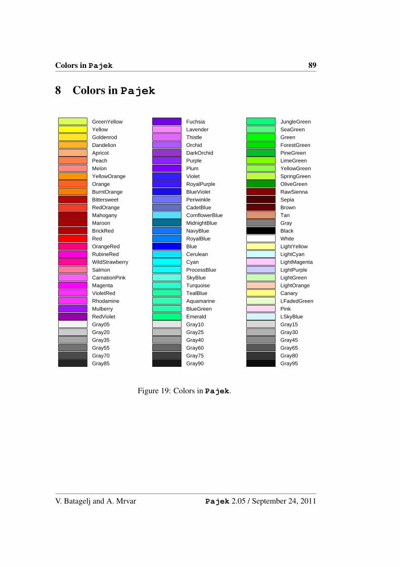
Colors in Pajek 89
8 Colors in Pajek
GreenYellow
Yellow
Goldenrod
Dandelion
Apricot
Peach
Melon
YellowOrange
Orange
BurntOrange
Bittersweet
RedOrange
Mahogany
Maroon
BrickRed
Red
OrangeRed
RubineRed
WildStrawberry
Salmon
CarnationPink
Magenta
VioletRed
Rhodamine
Mulberry
RedViolet
Fuchsia
Lavender
Thistle
Orchid
DarkOrchid
Purple
Plum
Violet
RoyalPurple
BlueViolet
Periwinkle
CadetBlue
CornflowerBlue
MidnightBlue
NavyBlue
RoyalBlue
Blue
Cerulean
Cyan
ProcessBlue
SkyBlue
Turquoise
TealBlue
Aquamarine
BlueGreen
Emerald
JungleGreen
SeaGreen
Green
ForestGreen
PineGreen
LimeGreen
YellowGreen
SpringGreen
OliveGreen
RawSienna
Sepia
Brown
Tan
Gray
Black
White
LightYellow
LightCyan
LightMagenta
LightPurple
LightGreen
LightOrange
Canary
LFadedGreen
Pink
LSkyBlue
Gray05 Gray10 Gray15
Gray20 Gray25 Gray30
Gray35 Gray40 Gray45
Gray55 Gray60 Gray65
Gray70 Gray75 Gray80
Gray85 Gray90 Gray95
Figure 19: Colors in Pajek.
V. Batagelj and A. Mrvar Pajek 2.05 / September 24, 2011

90 Colors in Pajek
0 - Cyan
1 - Yellow
2 - LimeGreen
3 - Red
4 - Blue
5 - Pink
6 - White
7 - Orange
8 - Purple
9 - CadetBlue
10 - TealBlue
11 - OliveGreen
12 - Gray
13 - Black
14 - Maroon
15 - LightGreen
16 - LightYellow
17 - Magenta
18 - MidnightBlue
19 - Dandelion
20 - WildStrawberry
21 - ForestGreen
22 - Salmon
23 - LSkyBlue
24 - GreenYellow
25 - Lavender
26 - LFadedGreen
27 - LightPurple
28 - CornflowerBlue
29 - LightOrange
30 - Tan
31 - LightCyan
32 - Gray20
33 - Gray60
34 - Gray40
35 - Gray75
36 - Gray10
37 - Gray85
38 - Gray30
39 - Gray70
Figure 20: Partition colors.
V. Batagelj and A. Mrvar Pajek 2.05 / September 24, 2011
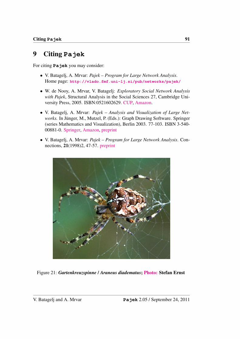
Citing Pajek 91
9 Citing PajekFor citing Pajek you may consider:
• V. Batagelj, A. Mrvar: Pajek – Program for Large Network Analysis.Home page: http://vlado.fmf.uni-lj.si/pub/networks/pajek/
• W. de Nooy, A. Mrvar, V. Batagelj: Exploratory Social Network Analysiswith Pajek, Structural Analysis in the Social Sciences 27, Cambridge Uni-versity Press, 2005. ISBN:0521602629. CUP, Amazon.
• V. Batagelj, A. Mrvar: Pajek – Analysis and Visualization of Large Net-works. In Junger, M., Mutzel, P. (Eds.): Graph Drawing Software. Springer(series Mathematics and Visualization), Berlin 2003. 77-103. ISBN 3-540-00881-0. Springer, Amazon, preprint
• V. Batagelj, A. Mrvar: Pajek – Program for Large Network Analysis. Con-nections, 21(1998)2, 47-57. preprint
Figure 21: Gartenkreuzspinne / Araneus diadematus; Photo: Stefan Ernst
V. Batagelj and A. Mrvar Pajek 2.05 / September 24, 2011

92 References
References[1] Adobe SVG viewer. http://www.adobe.com/svg/
http://www.adobe.com/svg/viewer/install
[2] Ahmed, A., Batagelj, V., Fu, X., Hong, S.-H., Merrick, D., Mrvar, A. (2007):Visualisation and analysis of the Internet movie database. Asia-Pacific Sym-posium on Visualisation 2007 (IEEE Cat. No. 07EX1615), 17-24.
[3] Albert R., Barabasi A.L.: Topology of evolving networks: local events anduniversality.http://xxx.lanl.gov/abs/cond-mat/0005085
[4] Batagelj V.: Papers on network analysis.http://vlado.fmf.uni-lj.si/pub/networks/doc/
[5] Batagelj V.: Workshop on Network Analysis, Sydney, Australia: 14th to17th June 2005; at Nicta (National ICT Australia).http://vlado.fmf.uni-lj.si/pub/networks/doc/#NICTA
[6] Batagelj V.: Some new procedures in Pajek. Dagstuhl seminar 05361,Dagstuhl, Germany, Sept 5-9, 2005.http://vlado.fmf.uni-lj.si/pub/networks/doc/dagstuhl/NewProcs.pdf
[7] Batagelj, V. (1997) Notes on blockmodeling. Social Networks 19, 143-155.
[8] Batagelj V.: Efficient Algorithms for Citation Network Analysis.http://arxiv.org/abs/cs.DL/0309023
[9] Batagelj V.: MODEL 2. http://vlado.fmf.uni-lj.si/pub/networks/
[10] Batagelj V. (2009): Social Network Analysis, Large-Scale. R.A. Meyers, ed.,Encyclopedia of Complexity and Systems Science, Springer 2009: 8245-8265. http://www.springerlink.com/content/tp3w7237m4624462/
[11] Batagelj V. (2009): Complex Networks, Visualization of. R.A. Meyers, ed.,Encyclopedia of Complexity and Systems Science, Springer 2009: 1253-1268. http://www.springerlink.com/content/m472707688618h17/
[12] Batagelj V., Brandes U. (2005): Efficient Generation of Large Random Net-works. Physical Review E 71, 036113, 1-5.
[13] Batagelj, V., Ferligoj, A., and Doreian, P. (1992), Direct and Indirect Meth-ods for Structural Equivalence, Social Networks, 14, 63–90.
V. Batagelj and A. Mrvar Pajek 2.05 / September 24, 2011

References 93
[14] Batagelj, V., Doreian, P., and Ferligoj, A. (1992) An Optimizational Ap-proach to Regular Equivalence. Social Networks 14, 121-135.
[15] Batagelj, V, Ferligoj, A, Doreian, P (2007): Indirect blockmodeling of 3-waynetworks. Selected contributions in data analysis and classification, Springer,Berlin, 151-159.
[16] Batagelj, V., Kejzar, N., Korenjak-Cerne, S. (2008): Analysis of the Cus-tomers? Choice Networks: An Application on Amazon Books and CDsData. Metodoloski zvezki/Advances in Methodology and Statistics 4 (2):191-204.
[17] Batagelj V., Mrvar A.: Pajek.http://vlado.fmf.uni-lj.si/pub/networks/pajek/
[18] Batagelj V., Mrvar A. (2000) Some Analyses of Erdos Collaboration Graph.Social Networks, 22, 173-186
[19] Batagelj V., Mrvar A. (2001) A Subquadratic Triad Census Algorithm forLarge Sparse Networks with Small Maximum Degree. Social Networks, 23,237-243
[20] Batagelj V., Mrvar A. (2008) Analysis of Kinship Relations With Pajek. So-cial Science Computer Review 26(2), 224-246, 2008.
[21] Batagelj V., Mrvar A., Zaversnik M. (1999) Partitioning Approach to Visual-ization of Large Graphs. In: Kratochvil J. (Ed.) GD’99, Stirin Castle, CzechRepublic. LNCS 1731. Springer-Verlag, 90-97.
[22] Batagelj V., Mrvar A., Zaversnik M. (2002) Network analysis of texts. Lan-guage Technologies, Ljubljana, p. 143-148.http://nl.ijs.si/isjt02/zbornik/sdjt02-24bbatagelj.pdf
[23] Batagelj V., Zaversnik M. (2011): Fast algorithms for determining (general-ized) core groups in social networks. Advances in Data Analysis and Classi-fication. Springer
[24] Batagelj, V. and Zaversnik, M. (2007): Short Cycles Connectivity. DiscreteMath 307 (3-5): 310-318.http://arxiv.org/abs/cs.DS/0308011
[25] Bollobas B.: Random Walks on Graphs,
[26] Broder A. etal. (2000): Graph structure in the web.http://www.almaden.ibm.com/cs/k53/www9.final/
V. Batagelj and A. Mrvar Pajek 2.05 / September 24, 2011

94 References
[27] Burt R.S. (1992): Structural Holes. The Social Structure of Competition.Cambridge MA: Harvard University Press.
[28] Butts, C.T. (2002) sna: Tools for Social Network Analysis.http://cran.at.r-project.org/src/contrib/PACKAGES.html#sna
[29] Cortona Player (2006)http://www.parallelgraphics.com/products/cortona/
[30] Cosmo Player (2002) http://ca.com/cosmo/
[31] de Nooy W., Mrvar A., Batagelj V. (2002) Exploratory Social Network Anal-ysis With Pajek. Structural Analysis in the Social Sciences 27, CambridgeUniversity Press, 2005. ISBN:0521602629. CUP, Amazon, Tokyo DenkiUniversity Press 2009.
[32] Doreian P., Mrvar A. (1996) A Partitioning Approach to Structural Balance.Social Networks, 18. 149-168
[33] Doreian, P., Batagelj, V., Ferligoj, A. (2000) Symmetric-acyclic decomposi-tions of networks. J. classif., 17(1), 3-28.
[34] Doreian P., Batagelj V., Ferligoj A. (2004) Generalized blockmodeling oftwo-mode network data. Social Networks 26, 29-53.
[35] Doreian P., Batagelj V., Ferligoj A.: Generalized Blockmodeling, Struc-tural Analysis in the Social Sciences 25, Cambridge University Press, 2005.ISBN:0521840856. CUP, Amazon.
[36] Dremelj P., Mrvar A., Batagelj V. (2002) Analiza rodoslova dubrovackogvlasteoskog kruga pomocu programa Pajek. Anali Dubrovnik XL, HAZU,Zagreb, Dubrovnik, 105-126 (in Croat).
[37] GEDCOM 5.5.http://homepages.rootsweb.com/˜pmcbride/gedcom/55gctoc.htm
[38] Ghostscript, Ghostview and GSview. http://www.cs.wisc.edu/˜ghost/
[39] Gibbons A. (1985) Algorithmic Graph Theory. Cambridge University Press.
[40] Grossman J. (2002) The Erdos Number Project.http://www.oakland.edu/˜grossman/erdoshp.html
[41] Hall, B.H., Jaffe, A.B. and Tratjenberg M.: The NBER U.S. Patent CitationsData File. NBER Working Paper 8498 (2001).http://www.nber.org/patents/
V. Batagelj and A. Mrvar Pajek 2.05 / September 24, 2011

References 95
[42] Hamberger, K., Houseman, M., Daillant, I., White, D.R., Barry, L. (2004)Matrimonial Ring Structures. Math. & Sci. hum. / Mathematics and SocialSciences, 42(4), 83-119.http://www.ehess.fr/revue-msh/pdf/N168R965.pdf
[43] Hummon, N.P., Doreian, P. (1989) Connectivity in a citation network: Thedevelopment of DNA theory. Social Networks, 11, 39–63.
[44] Jones B. (2002). Computational geometry database.http://compgeom.cs.uiuc.edu/˜jeffe/compgeom/biblios.html
[45] Kejzar, N., Korenjak Cerne, S., Batagelj, V. (2010) Network Analysis ofWorks on Clustering and Classification from Web of Science. Classificationas a Tool for Research. Hermann Locarek-Junge, Claus Weihs eds. Proceed-ings of IFCS 2009. Studies in Classification, Data Analysis, and KnowledgeOrganization, Part 3, 525-536, Springer, Berlin, 2010. Springer, preprint
[46] Kejzar, N., Nikoloski, Z., Batagelj, V. (2008): Probabilistic InductiveClasses of Graphs. Journal of Mathematical Sociology 32: 85-109.
[47] Kleinberg J. (1998) Authoritative sources in a hyperlinked environment. InProc 9th ACMSIAM Symposium on Discrete Algorithms, p. 668-677.http://www.cs.cornell.edu/home/kleinber/auth.ps
[48] Knuth, D. E. (1993) The Stanford GraphBase. Stanford University, ACMPress, New York. ftp://labrea.stanford.edu/pub/sgb/
[49] LOCKS: CRA Analyses of News Stories on the Terrorist Attack. ArizonaState University. http://locks.asu.edu/terror/
[50] McCabe, T. Computer Science Approaches: Visualization Tools andSoftware Metrics. in Survey Automation. NAP, 2003, p. 116-136.http://books.nap.edu/books/0309089301/html/116.html
[51] MDL Information Systems, Inc. (2002) http://www.mdli.com/
[52] James Moody home page (2002)http://www.soc.sbs.ohio-state.edu/jwm/
[53] Murtagh, F. (1985) Multidimensional Clustering Algorithms, Compstat lec-tures, 4, Vienna: Physica-Verlag.
[54] Pajek’s datasets:http://vlado.fmf.uni-lj.si/pub/networks/data/
V. Batagelj and A. Mrvar Pajek 2.05 / September 24, 2011

96 References
[55] D.M. Pennock etal. (2002) Winners dont’t take all, PNAS, 99/8, 5207-5211.
[56] Peterson J. L.: Petri Net Theory and the Modeling of Systems.
[57] The R Project for Statistical Computing. http://www.r-project.org/
[58] Richardson D.C., Richardson J.S. (2002) The Mage Page.http://kinemage.biochem.duke.edu/index.html
[59] Scott, J. (2000) Social Network Analysis: A Handbook, 2nd edition. Lon-don: Sage Publications.
[60] Seidman S. B. (1983) Network structure and minimum degree, Social Net-works, 5, 269–287.
[61] Tarjan, R. E. (1983) Data Structures and Network Algorithms. Society forIndustrial and Applied Mathematics Philadelphia, Pennsylvania.
[62] UCINET (2002) http://www.analytictech.com/
[63] The United States Patent and Trademark Office.http://patft.uspto.gov/netahtml/srchnum.htm
[64] Wasserman S., Faust K. (1994). Social Network Analysis: Methods and Ap-plications. Cambridge University Press, Cambridge.
[65] White D.R., Batagelj V., Mrvar A. (1999) Analyzing Large Kinship and Mar-riage Networks with Pgraph and Pajek. Social Science Computer Review,17 (3), 245-274
[66] Wilson, R.J., Watkins, J.J. (1990) Graphs: An Introductory Approach. NewYork: John Wiley and Sons.
[67] W3C SVG page. http://www.w3.org/Graphics/SVG
V. Batagelj and A. Mrvar Pajek 2.05 / September 24, 2011