program for automatic numerical conversion of a line graph

25

Letter

Program for Automatic Numerical Conversion of a Line Graph (Line Plot)

Michiko Yoshitake*, takashi kono, takuya kadohira

national institute for Materials science, 1-1, namiki, tsukuba, ibaraki, 305-0044 Japan*e-mail:[email protected]

(received: July 8, 2020; accepted for publication: september 17, 2020; online publication: october 27, 2020)

A program for fully automatic conversion of line plots in scientific papers into numerical data has been developed. By the conversion of image data into numerical data, users can treat so-called 'spectra' such as X-ray photoelectron spectra and optical absorption spectra in their purpose, plotting them in different ways such as inverse of wave number, subtracting them from users' data, and so forth. This article reports details of the program consisting of many parts, with several deep-learning models with different functions, elimination of literal characters, color separation, etc. Most deep-learning models achieve accuracy higher than 95%. The usability is demonstrated with some examples.

Keywords: image data, numerical data, automatic conversion, deep learning, Plot with multiple line

1 Introduction

the program (named "waveform digitizer") is designed

to convert line plots in scientific papers, books, and other

resources into numerical data so that one can use those

data numerically in plots as references. For example, using

numerical data from a line plot image of the temperature

dependence of dielectric constant, one can re-plot temperature

as abscissa and the inverse of (dielectric constant −1) and

obtain a slope of the plot, which corresponds to the Curie

constant. Another example is that by numerical conversion of

a plot in a paper, user can plot the converted data with user's

own data in the same figure as a reference for comparison,

or use the converted data for numerical process such as

subtraction, synthesis, and deconvolution of spectra.

some commercially available digitizer programs exist, but

they require users to operate in some part manually, such as

inputting parameters. By contrast, the program developed

as described herein is fully automatic; users need not sit in

front of a computer. This program has been developed in this

way because it is implemented in the FigureResourceMiner

of TextDataManagement system (TDM-FRM) of the NIMS

Materials data Platform [1–3], by which users can download

numerical data of a line graph (line plot) from a scientific

journal as a CSV [4] file. Figure 1(a) presents the whole tdM-

FRM system schematically. The program of this article, used

for pre-treatment in TDM-FRM system, is noted as "this

program" in the Figure. When a user of TDM-FRM system

selects a certain line graph of interest, a window such as

Figure 1(b) appears. The selected graph with its figure caption

is shown. By clicking a button on the upper-right side of the

window, the corresponding CsV file will be downloaded to

the user's computer. In the TDM-FRM system, image files in

XML [5] files of scientific papers are extracted, converted into

png format [6], and stored in a specific folder. The program

reads these png files, selects png files that are the subject of

digitalization, digitizes files, and saves digitized numerical

data in the specific folder as CSV files. The whole process

from reading png files to saving numerical data in CSV files is

done automatically in advance of users' access. The numerical

data which have already been converted are downloaded as a

CSV file upon the user's request.

At the time of writing this article, TDM-FRM is available

DOI: 10.2477/jccj.2020-0002

J. Comput. Chem. Jpn., Vol. 19, No. 2, pp. 25–35 (2020) ©2020 society of Computer Chemistry, Japan

http://dx.doi.org/10.2477/jccj.2020-0002

26 J. Comput. Chem. Jpn., Vol. 19, No. 2

Figure 1. (a) Schematic illustration of whole TDM-FRM system. Text data and Image data are imported and pre-treated first, and text data, information on the structure of text data are processed using 'elasticsearch' and 'Neo4j' (names of software). All data are stored in hard disc (HDD). (b) Example of a window that opens when a user selects a certain line graph of interest on TDM-FRM system.

27DOI: 10.2477/jccj.2020-0002

only to NIMS staff because of a contract with publishers about

the use of the source XML files. Nevertheless, this program

alone will be open to the public upon publication of the paper

through Material data repository (Mdr) of Materials data

Platform so that users outside of niMs can digitize their

png files. The program is written in Python [7]. Detailed

information [8] for users who would like to use the program

outside TDM-FRM will be posted on MDR.

2 Program

2.1 Types of plots for digitizingThe program digitizes a line plot. There are many png files

that do not form a line plot in the specific folder where png

films are stored. Therefore, a png file intended for digitizing

is selected in the first step of the program. At this moment, an

image that has multiple line plots in one png file is out of the

target for digitalization. In addition, the following conditions

must be satisfied for digitization with this program: have a

clear drawing of the x-axis and y-axis, the y-axis should be on

the left side of the plot, and a plot should be drawn with line

(so-called a line plot with/without symbols, not a fitted line).

In Figure 2, examples of graphs that can be digitized with

this program (a) or not (b), are shown. A bar graph (top left

of Figure 2(b), fitted line graphs (bottom left), a line plot that

has multiple y values for one x value (top middle), a line plot

without y axis (bottom middle), a plot with symbols without

lines (top right), and multiple plots in one png file (bottom

right), are not converted into numerical data with this program.

2.2 Overall designFigure 3 shows the overall design of the program, where an

image file in png format is entered, treated in a computer with

many algorithms, and finally converted numerical data is saved

in the CSV format. The entire program is written with Python

3.6 [9] and Keras [10], with the Tensorflow [11] backend used

for deep learning.

Figure 2. Examples of graphs that can be converted with this program (a) or not (b). See text for more explanations.


At first, a png image file is screened, where appropriate line

plot images for digitizing (deep-learning model a is used)

are determined. The file name of the selected image is stored

temporarily for later use. Characters such as numeric symbols

and alphabets are eliminated from the selected image using

OCR (Tesseract OCR [12]). Since the pixel size should be

normalized for all images for deep learning [13], image size is

normalized several times in the flow of the program. The main

operation, except for deep learning in the flow, is dividing

the image according to color, where the number of colors in

the image is determined automatically using density-based

spatial clustering of applications with noise (dBsCan [14],

implemented in a scikit-learn module [15] is used). Through

this process, all line plots in one png image are converted into

multiple images for each color in gray scale. The multiple

images in gray scale undergo the same process in the program

hereinafter (irrespective of the colors in the original images).

the size used for digitizing, 1024× 1024 pixels, was chosen

for two reasons. The first is that many scientific journals

request that authors use images with 600 dpi (dots per inch) or

better resolution, which in a paper appears as approximately

1200 dots (= pixels) per column width for a whole image

including the plot scales and labels, resulting in nearly 1000

pixels in lateral direction of the plot area. Because a size that

matches 2n form (n is an integer) is preferred for computing,

1024 pixels was chosen. The second reason derives simply

from computer performance, memory resource limitations, and

computing time. It is noteworthy that images with reduced size

(360 × 360) are used in dBsCan because of the limitations

in the DBSCAN module itself. In deep learning parts, images

with reduced size are also used in some parts, as described in

the following deep learning part.

the values obtained after digitizing with deep learning are

normalized between zero to one for both the abscissa and

Figure 3. Schematic overall design of the program.

29DOI: 10.2477/jccj.2020-0002

ordinate. Subsequently, these values are re-scaled with values

obtained by calculating the true scales in the original images

using OCR (pyocr [16]), which will be described in 2.4.

2.3 Deep learning partsFor different purposes, five deep learning models were

produced. ResNet [17] is used for models A, B, D, and E as a

base model. For model C, in which both input and output are

images in the same size, U-Net [18] is used as a base model.

each model is given as a supplement, whose name is listed in

table 1. The accuracy calculated with test data is given as a

measure of the performance of each model, where the accuracy

is defined as (true positive + true negative) divided by (true

positive + false negative + false positive + true negative). Brief

explanation on training data formation is mentioned in the

paper, but details for users who would like to produce training

data and make deep learning model by themselves, would be

better understood by reading the source code of the program

[8].

the image selection model, a, is trained using labeled

training data such as those in Figure 4(b). Each image pixel

size of the original images (X0, Y0) differs as shown in

Figure 4(a). Therefore, all images should be normalized to

the same size before deep learning. Because high resolution

is not necessary when merely selecting images, image size

is reduced to 256 × 256 pixels. In addition, color images are

gray scaled to save memory resources and computation time.

after selecting images (actually, the file name is passed to

the main program), images with 1024 × 1024 pixels are used

for subsequent treatments. The labeled training data consist

of normalized image data with ground truth (correct answer

label). For images subject to digitizing, ground truth is "1";

otherwise it is "0", which were labeled manually. The image

data for training were extracted randomly from png files in the

XML dataset (14 TB) our institute purchases from publishers.

Because images with ground truth "1" (1794 images) are

much fewer than those with "0" (5238 images), 4500 images

with ground truth "1" were generated using a computer in the

way described in the section of Digitize model E. The model

accuracy has been 0.95.

origin and axis length prediction model B is to find the

origin position and lengths of axes within individual image

pixels. In a 1024 × 1024 pixel image, a plot area can be

located in many ways: pixels of margins, width of scale and

label on an axis can be different for each image, as shown

on the left side of Figure 5. To extract a plot area, the origin

position (left most and lower half of the plot), (Xorg,Yorg) and

the x-axis and y-axis lengths (Lx,Ly) are machine-learned. The

training data are generated using a computer. With a randomly

chosen origin position in pixel units (in the lower left quarter

of the image) and x-axis and y-axis lengths in pixel units, a

line plot image has been drawn as an input of training data.

the origin and lengths used to draw the image are ground

truth. In all, 10,000 data were generated, of which 9,000 were

used as training data; the rest were used as test data. For this

model, the ground truth origin and axis lengths were handled

individually at the last part of the neural network layer (see

supplement for details) to improve accuracy. The respective

accuracies of the origin and axis lengths were 0.966 and 0.997.

here, "true" indicates that an absolute value of (predicted data

− test data) divided by test data is equal to or less than 0.03 for

both the x-axis and y-axis.

Forming model C is designed to eliminate grid lines and

annotations in the plot that have not been eliminated in

the precedent process (see Figure 3). Figure 6 presents the

appearance of the training data. Input data for this model are

gray scale. Training data were generated using a computer

in the following way: Ground truth image data are generated

using Gauss function described in the section of digitize

model E. Input data are generated by adding either grid lines

or annotations to the ground truth image data. 5,000 training

data were generated, of which 4,000 were used for training and

the rest for a test. The training data were limited for reasons

of computer performance. The accuracy of model C has been

0.78, where the sum of pixel value difference between training

data and ground truth divided by the sum of the pixel value of

Table 1. List of file names of deep learning models in supple-ment materials.

model a 1_FigSelection_256_RN34.pngmodel B 2_OrgAxl_1024_RN26.pngmodel C 3_Shaping_1024_U-Net.pngmodel d 4_LineNum_360_RN34.pngmodel e 1 5_Digitizer_1-line_1024_RN34.png

2 5_Digitizer_2-lines_1024_RN26.png3 5_Digitizer_3-lines_1024_RN26.png


Figure 4. (a) Examples of original data for digitization. (b) Examples of training data for Image selection model, A. Original image in (a) is converted to gray scale and pixel size for all images is changed to 256 × 256.

31DOI: 10.2477/jccj.2020-0002

Figure 5. Examples of training data for Origin and axis length prediction model, B. A pattern between the image and the position of the origin in x and y direction and axis length in x and y direction, is to be learned.

Figure 6. Examples of training data for Forming model, C. A pattern between input image and ground truth image (unnecessary part is eliminated) is to be learned.


the ground truth (all in gray scale, pixel value is between zero

and 255 depending on pixel contrasting density) was used as

an error. If the absolute value of the error exceeded 0.1, it was

judged as "false".

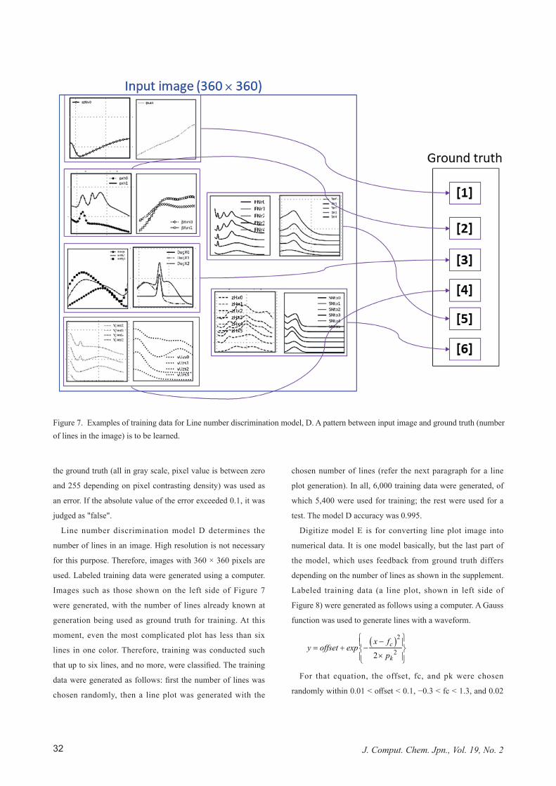
Line number discrimination model d determines the

number of lines in an image. High resolution is not necessary

for this purpose. Therefore, images with 360 × 360 pixels are

used. Labeled training data were generated using a computer.

Images such as those shown on the left side of Figure 7

were generated, with the number of lines already known at

generation being used as ground truth for training. At this

moment, even the most complicated plot has less than six

lines in one color. Therefore, training was conducted such

that up to six lines, and no more, were classified. The training

data were generated as follows: first the number of lines was

chosen randomly, then a line plot was generated with the

chosen number of lines (refer the next paragraph for a line

plot generation). In all, 6,000 training data were generated, of

which 5,400 were used for training; the rest were used for a

test. The model D accuracy was 0.995.

digitize model e is for converting line plot image into

numerical data. It is one model basically, but the last part of

the model, which uses feedback from ground truth differs

depending on the number of lines as shown in the supplement.

Labeled training data (a line plot, shown in left side of

Figure 8) were generated as follows using a computer. A Gauss

function was used to generate lines with a waveform.

( )2

22c

k

x fy offset exp

p

− = + − ×

For that equation, the offset, fc, and pk were chosen

randomly within 0.01 < offset < 0.1, −0.3 < fc < 1.3, and 0.02

Figure 7. Examples of training data for Line number discrimination model, D. A pattern between input image and ground truth (number of lines in the image) is to be learned.

33DOI: 10.2477/jccj.2020-0002

< pk < 0.3. After generating one line in the above manner

(parameters are denoted as offset (1), fc (1) and pk (1)),

successive lines generated with parameters listed in table 2

were used as waveforms.

after all waveforms were generated, numerical values were

normalized with the maximum value of all the values so that

data for all lines are within 0–1. Ground truth is a series of a

row of 1024 numbers used to generate the image. For a one-

line plot, ground truth is one row of 1024 numbers. Ground

truth for a two-line plot is two rows of 1024 numbers, which

consists of 1024 × 2 numbers, and so forth. For the moment,

training has been done up to a three-line plot. Training

for more multi-line plot is easy in a technical sense, but it

consumes large amounts of time. Because few plots have more

Figure 8. Examples of training data for Digitize model, E. A pattern between input image and ground truth (numerical data of the plot) is to be learned.

Table 2. Range of values of parameters in the equation.

offset fc pkfirst line 0.01 < offset (1) < 0.1 -0.3 < fc (1) < 1.3 0.02 < pk (1) < 0.3second line offset (2) = offset (1) + Δoffset (2) fc (2) = fc (1) +Δfc (2) pk (2) = pk (1)· Δpk (2)

0.1 < Δoffset (2) < 0.5 -0.03 < Δfc (2) < 0.03 0.5 < Δpk (2) < 2third line offset (3) = offset (1) + Δoffset (3) fc (3) = fc (1) +Δfc (3) pk (3) = pk (1)· Δpk (3)

0.1 < Δoffset (3) < 0.5 -0.03 < Δfc (3) < 0.03 0.5 < Δpk (3) < 2fourth line offset (4) = offset (1) + Δoffset (4) fc (4) = fc (1) +Δfc (4) pk (4) = pk (1)· Δpk (4)

0.1 < Δoffset (4) < 0.5 -0.03 < Δfc (4) < 0.03 0.5 < Δpk (4) < 2fifth line offset (5) = offset (1) + Δoffset (5) fc (5) = fc (1) +Δfc (5) pk (5) = pk (1)· Δpk (5)

0.1 < Δoffset (5) < 0.5 -0.03 < Δfc (5) < 0.03 0.5 < Δpk (5) < 2sixth line offset (6) = offset (1) + Δoffset (6) fc (6) = fc (1) +Δfc (6) pk (6) = pk (1)· Δpk (6)

0.1 < Δoffset (6) < 0.5 -0.03 < Δfc (6) < 0.03 0.5 < Δpk (6) < 2


than four-lines in one color, training for and more than four-

lines has been halted. A schematic illustration of training data

variation is presented in Figure 8. 10,000 training data were

generated, of which 9,000 were used for training. The rest

were used for testing. The accuracies of model E were found

to be 0.96, 0.82, and 0.60, respectively, for a one-line plot,

two-line plot, and three-line plot. Here, "true" means that the

maximum value among an absolute value of (predicted data −

test data) divided by test data calculated for each data point is

equal to or less than 0.03 for all lines in one image.

2.4 Re-scalingas already mentioned, numerical data obtained by digitize

model e are normalized and have values between zero to

1. These values should be re-scaled to the true scale of

the original plot image. For re-scaling, the minimum and

maximum values of x-axis scale and y-scale are extracted

using OCR (pyocr [16]) in the following way. Numerical

characters below the x-axis line are regarded as x-scale, and

the pixel position in x-direction of the characters are detected.

among extracted characters, the pixel position of the minimum

number (x1) in x-direction X1 and the pixel position of the

maximum number (x2) in x-direction X2 are used to calculate

the minimum value (xmin) and maximum value (xmax) of x-axis

with the following equations.

( )0

1 01 2 1 0

2 1 ,

1024mim orgX X Xx x x x X XX X

−= − × − = ×

−

( )0

0 22 2 1

2 1 ,

1024L

max L xX X X Xx x x x X L

X X+ −

= + × − = ×−

the equations corresponding to y-axis are used to calculate

values of ymin and ymax. Then, numerical data obtained by

digitize model e are re-scaled so that the minimum and

maximum values have the above calculated values.

3 Examples of conversion

Figure 9 portrays an example of digitalization of a line

plot with three lines in different colors. Figure 9(a) shows the

original line plot as a png file. For this plot, three images are

generated inside the program: one for blue, one for red, and

the other for black. Each image is converted into gray scale.

among the described processes, in the digitizing process with

deep learning model e for one row is conducted because there

is only one line for each color. A file with three rows, each

corresponding to blue, red, and black lines, is saved as a CsV

file. A reconstructed line plot from the CSV file is depicted in

Figure 9(b). Reproducibility of both x-scale and y-scale is not

bad. The reconstructed line plot always appears to be smooth

because no noise-like peak has been trained. Figure 10 presents

another example of digitalization. Here, the y-axis scale of the

original line plot is arbitrary, as presented in Figure 10(a). The

program normalizes the length of the axis into a number from

0 to 1, as presented in Figure 10(b) if the scale is arbitrary.

When lines with different colors overlap in the original

image, the color of overlapped pixels becomes different from

the original one. Such a pixel is dropped (regarded as a white

pixel) when the image is divided into images for each color;

the color lines are therefore discontinuous. Color lines are not

continuous if the original color lines are dotted or broken lines.

to digitize such discontinuous lines, digitize model e has a

function to compensate for missing parts of lines.

Figure 9. Digitalization of a line plot with three lines in differ-ent colors. (a) is the original image in png format and (b) is a plot made from numerical values digitized by the program.

35DOI: 10.2477/jccj.2020-0002

4 Summary

a program has been developed for fully automatic

conversion of line plots in scientific papers into numerical

data. In advance of conversion, a line plot should be extracted

as png files from an original XML file of a paper. Converted

numerical data are given as CSV files. The program consists

of many parts with different functions: elimination of literal

characters, color separation, five deep learning models (the

image selection model for selecting line plots from various

png images, the origin and axis length prediction model for

detecting real line plot pixel area, the Forming model for

eliminating grid lines or annotations in the plot, the Line

number discrimination model for finding a number of lines

for each color, and the digitize model for converting into

numerical data), and so forth. Most deep learning models

achieved more than 95% accuracy in test data, which can

be improved through further computation. Examples of

conversion show a satisfactory level of digitization.

References

[1] M. Tanifuji, A. Matsuda, H. Yoshikawa, Proceedings of advanced applied informatics, iiai international Conference, July 2019

[2] https://www.nims.go.jp/eng/research/materials-data-pf/index.html

[3] T. Kadohira, S. Kikuchi, K. Sakamoto, H. Naito, M. Tanifuji, Conference on a Fair Data Infrastructure for Materials Genomics, 3 − 5 June, 2020, virtual meeting.

[4] CsV, (comma separated values) is a data format where each value or item is separated by comma. More explanations at https://www.ietf.org/rfc/rfc4180.txt

[5] XML, (extensible markup language) is a markup language that defines a set of rules for encoding documents in a format that is both human-readable and machine-readable. World Wide Web Consortium defines the rules. More explanations at https://www.w3.org/TR/xml11/#sec-xml11

[6] png (portable network graphics) format is one of file formats for handling bitmap images such as GIF, TIFT, and JPEG. Png is license-free format.

[7] pyhton is a programming language that has many modules for machine learning, and free of use.

[8] https://mdr.nims.go.jp/concern/publications/df65v866p [9] https://www.python.org/downloads/release/python-368/ [10] Keras is a module for describing simplified deep learning

models. More explanations at https://keras.io/ja/ [11] Tensorflow is an open source software library for

machine learning and can be downloaded from https://github.com/tensorflow/tensorflow

[12] oCr, (optical character recognition) is a software to convert images of characters into character codes. tesseract oCr is one of free software downloadable from https://github.com/tesseract-ocr/

[13] deep learning is one of machine learning techniques using multiple layer neural network.

[14] dBsCan, (density-based spatial clustering of applications with noise) is one of algorithms for data clustering. More explanations at https://en.wikipedia.org/wiki/DBSCAN

[15] scikit-learn is a free software machine learning library for the Python programming language, which includes a module for DBSCAN. More explanations at https://scikit-learn.org/stable/modules/generated/sklearn.cluster.DBSCAN.html

[16] pyocr is a free OCR software. More explanations at https://pypi.org/project/pyocr/

[17] resnet (residual networks) is a neural network architecture used for image recognition. More explanations at http://torch.ch/blog/2016/02/04/resnets.html

[18] U-net is convolutional network architecture for fast and precise segmentation of images. More explanations at https://arxiv.org/abs/1505.04597

Figure 10. Digitalization of a line plot with arbitrary y-scale in the original image. (a) is the original image in png format and (b) is a plot made from numerical values digitized by the program.

program for automatic numerical conversion of a line graph

Documents