Progress in Mathematical PhysicsVolume 51

Editors-in-Chief

Anne Boutet de Monvel, Universite Paris VII Denis DiderotGerald Kaiser, Center for Signals and Waves, Austin, TX

Editorial Board

C. Berenstein, University of Maryland, College ParkSir M. Berry, University of BristolP. Blanchard, Universitat BielefeldM. Eastwood, University of AdelaideA.S. Fokas, University of CambridgeC. Tracy, University of California, Davis

Diarmuid O Mathuna

Integrable Systems inCelestial Mechanics

Birkhauser

Boston • Basel • Berlin

Diarmuid O MathunaDublin Institute of Advanced Studies10, Burlington RoadDublin, 4.Irelandomathuna@stp.dias.ie

ISBN-13: 978-0-8176-4096-5 e-ISBN-13: 978-0-8176-4595-3DOI: 10.1007/978-0-8176-4595-3

Library of Congress Control Number: 2008925448

Mathematics Subject Classification (2000): 34A05, 70-XX, 70-02, 70F05, 70F15, 70H06, 70M20,85-02

c ¨All rights reserved. This work may not be translated or copied in whole or in part without thewritten permission of the publisher (Birkhauser Boston, c/o Springer Science+Business Media,LLC, 233 Spring Street, New York, NY 10013, USA), except for brief excerpts in connection withreviews or scholarly analysis. Use in connection with any form of information storage and re-trieval, electronic adaptation, computer software, or by similar or dissimilar methodology nowknown or hereafter developed is forbidden.The use in this publication of trade names, trademarks, service marks and similar terms, evenif they are not identified as such, is not to be taken as an expression of opinion as to whether ornot they are subject to proprietary rights.

Typeset by Martin Stock in LATEX.

Printed on acid-free paper.

9 8 7 6 5 4 3 2 1

www.birkhauser.com

©2008 Birkhauser Boston, a part of Springer Science + Business Media, LLC

I gcuimhne ar mo thuismitheoirı(To the memory of my parents)

Contents

Preface . . . . . . . . . . . . . . . . . . . . . . . . . . . . . . . . . . . . . . . . . . . . . . . . . . . . . . . . . . . . ix

0 General Introduction . . . . . . . . . . . . . . . . . . . . . . . . . . . . . . . . . . . . . . . . . . . . . . . 1

1 Lagrangian Mechanics . . . . . . . . . . . . . . . . . . . . . . . . . . . . . . . . . . . . . . . . . . . . . . 211 Lagrangian Systems . . . . . . . . . . . . . . . . . . . . . . . . . . . . . . . . . . . . . . . . . . . . . . . 212 Ignorable Coordinates . . . . . . . . . . . . . . . . . . . . . . . . . . . . . . . . . . . . . . . . . . . . . 223 Separable Systems . . . . . . . . . . . . . . . . . . . . . . . . . . . . . . . . . . . . . . . . . . . . . . . . . 244 Liouville Systems . . . . . . . . . . . . . . . . . . . . . . . . . . . . . . . . . . . . . . . . . . . . . . . . . . 26

2 The Kepler Problem . . . . . . . . . . . . . . . . . . . . . . . . . . . . . . . . . . . . . . . . . . . . . . . . 291 Features of the Ellipse: Geometry and Analysis . . . . . . . . . . . . . . . . . . . . . 292 The Two-Body Problem . . . . . . . . . . . . . . . . . . . . . . . . . . . . . . . . . . . . . . . . . . . . 333 The Kepler Problem: Vectorial Treatment . . . . . . . . . . . . . . . . . . . . . . . . . . 354 The Kepler Problem: Lagrangian Analysis . . . . . . . . . . . . . . . . . . . . . . . . . . 41

3 The Euler Problem I — Planar Case . . . . . . . . . . . . . . . . . . . . . . . . . . . . . . . . . 491 The Gravitational Field of Two Fixed Centers: Planar Case . . . . . . . . . . 492 The Lagrangian in Liouville Form: The Energy Integral . . . . . . . . . . . . . . 513 The First Integrals in Liouville Coordinates . . . . . . . . . . . . . . . . . . . . . . . . 534 The First Integrals in Spheroidal Coordinates . . . . . . . . . . . . . . . . . . . . . . 545 Reduction of the Equations: The Regularizing Variable . . . . . . . . . . . . . 566 Some Particular Cases . . . . . . . . . . . . . . . . . . . . . . . . . . . . . . . . . . . . . . . . . . . . . 587 Analysis of the Generic Equation . . . . . . . . . . . . . . . . . . . . . . . . . . . . . . . . . . 628 The Equation for S = cosσ : Specification of Λ . . . . . . . . . . . . . . . . . . . . . . 659 The Equation for R . . . . . . . . . . . . . . . . . . . . . . . . . . . . . . . . . . . . . . . . . . . . . . . . 7710 The Time-Angle Relation . . . . . . . . . . . . . . . . . . . . . . . . . . . . . . . . . . . . . . . . . . 8811 The Complementary Range . . . . . . . . . . . . . . . . . . . . . . . . . . . . . . . . . . . . . . . . 9312 The Singular Case: C = 0 . . . . . . . . . . . . . . . . . . . . . . . . . . . . . . . . . . . . . . . . . . . 9813 Summary of the Orbit Solutions . . . . . . . . . . . . . . . . . . . . . . . . . . . . . . . . . . . 105

4 The Euler Problem II — Three-dimensional Case . . . . . . . . . . . . . . . . . . . . 1131 The Gravitational Field of Two Fixed Centers: General Case . . . . . . . . 1132 The Ignorable Coordinate: Liouville’s Form and the Energy Integral . 115

viii Contents

3 The First Integrals in Liouville Coordinates . . . . . . . . . . . . . . . . . . . . . . . . 1184 The First Integrals in Spheroidal Coordinates . . . . . . . . . . . . . . . . . . . . . . 1195 Reduction of Equations: The Regularization . . . . . . . . . . . . . . . . . . . . . . . . 1206 Normalization of the Quartics . . . . . . . . . . . . . . . . . . . . . . . . . . . . . . . . . . . . . 1217 The σ -equation in the Case β = 0 . . . . . . . . . . . . . . . . . . . . . . . . . . . . . . . . . . 1238 The R-equation . . . . . . . . . . . . . . . . . . . . . . . . . . . . . . . . . . . . . . . . . . . . . . . . . . . . 1259 The Integration of the Third (Longitude) Coordinate . . . . . . . . . . . . . . . 13310 The Time-Angle Relation . . . . . . . . . . . . . . . . . . . . . . . . . . . . . . . . . . . . . . . . . . 142

5 The Earth Satellite — General Analysis . . . . . . . . . . . . . . . . . . . . . . . . . . . . . . 1431 The Geopotential and the Density Distribution . . . . . . . . . . . . . . . . . . . . . 1432 The Vinti Potential . . . . . . . . . . . . . . . . . . . . . . . . . . . . . . . . . . . . . . . . . . . . . . . . 1473 The Vinti Dynamical Problem . . . . . . . . . . . . . . . . . . . . . . . . . . . . . . . . . . . . . . 1504 The Integration of the Lagrangian Equations . . . . . . . . . . . . . . . . . . . . . . . 1535 Reduction of the Equations; Regularization; Normalization . . . . . . . . . 1556 The σ -Equation: Definition of Λ . . . . . . . . . . . . . . . . . . . . . . . . . . . . . . . . . . . 1577 The R-Equation . . . . . . . . . . . . . . . . . . . . . . . . . . . . . . . . . . . . . . . . . . . . . . . . . . . . 1598 The Integration of the ϕ-Coordinate . . . . . . . . . . . . . . . . . . . . . . . . . . . . . . . 1729 The Time-Angle Relation . . . . . . . . . . . . . . . . . . . . . . . . . . . . . . . . . . . . . . . . . . 182

6 The Earth Satellite — Some Special Orbits . . . . . . . . . . . . . . . . . . . . . . . . . . . 1931 Orbits in the Near Equatorial Band . . . . . . . . . . . . . . . . . . . . . . . . . . . . . . . . . 1932 The Equatorial Orbit . . . . . . . . . . . . . . . . . . . . . . . . . . . . . . . . . . . . . . . . . . . . . . . 1963 The Polar Orbit . . . . . . . . . . . . . . . . . . . . . . . . . . . . . . . . . . . . . . . . . . . . . . . . . . . . 1994 The “Critical” Inclination . . . . . . . . . . . . . . . . . . . . . . . . . . . . . . . . . . . . . . . . . . 205

Appendix: Calculation and Exhibition of Orbits;The Time-Angle Relation . . . . . . . . . . . . . . . . . . . . . . . . . . . . . . . . . . . . . . . . . . . 2111 Orbits in Chapter 3 . . . . . . . . . . . . . . . . . . . . . . . . . . . . . . . . . . . . . . . . . . . . . . . . 2132 Orbits in Chapters 5 and 6. . . . . . . . . . . . . . . . . . . . . . . . . . . . . . . . . . . . . . . . . 2143 The Time-Angle Relation . . . . . . . . . . . . . . . . . . . . . . . . . . . . . . . . . . . . . . . . . . 2154 Orbits Derived from Given Initial Conditions in Chapter 3 . . . . . . . . . . 216

References . . . . . . . . . . . . . . . . . . . . . . . . . . . . . . . . . . . . . . . . . . . . . . . . . . . . . . . . . . . . 227

Index . . . . . . . . . . . . . . . . . . . . . . . . . . . . . . . . . . . . . . . . . . . . . . . . . . . . . . . . . . . . . . . . . 231

Preface

Direct involvement with the subject area of the present work dates from myyears with NASA at its Electronics Research Center (ERC) in Cambridge, Mas-sachusetts, in the 1960s. However, my approach to the problems of mathemat-ical physics had been shaped earlier in my time as a graduate student in theMathematics Department at MIT. The passage of time tends merely to furtherenhance my appreciation of that graduate study program, where I had the ben-efit of the intensive courses from Norman Levinson, C.-C. Lin, Jurgen Moser,and Eric Reissner. In the case of Reissner, my years as research assistant werea formative apprenticeship — one could say on the “shop-floor”.

The stimulus to organize my convictions in book form came from myfriends at Birkhauser Boston, and I wish to thank Ann Kostant for providingme with the opportunity and support in producing it; a special thanks goes toEdwin Beschler, formerly of Birkhauser, for his consistent encouragement overthe years.

In the course of writing, I had the good-humored support and invaluablehelp from my one-time teacher and long-time friend, Vincent Hart. He readeach chapter as it was written and his sharp eye picked up my many slipsand errors. More significantly, his persistent questioning on the original formof Chapter 3 forced me to address all parameter ranges and provide solutionforms to cover all possibilities for the case of negative energy.

He also raised the issue of providing illustrations of the various orbit types,a task I was reluctant to undertake. My only escape from the pressure wasto invite him to do that part — to which he readily agreed. At that point ayoung colleague, Sean Murray, provided his precious expertise with Maple; theAppendix is the product of their fruitful cooperation.

In dealing with some difficulties with Euler’s Latin, I had the ready assis-tance from the Medieval Latin team at the Royal Irish Academy, and I wish torecord my thanks to Anthony Harvey, Angela Malthouse, and Jane Power.

The heroic task of typesetting was performed by Martin Stock, and theexcellent layout of difficult material speaks for his committed perfectionism.Working from my manuscript was not easy, but his good humor prevailed overall difficulties. As one progresses into the script, the going does not get any

x Preface

easier, but Martin’s professionalism ensured that he finished with a flourish.For such an accomplishment, I am at a loss for words to adequately expressmy appreciation.

With such help and support, what deficiencies remain must be my soleresponsibility.

Diarmuid O MathunaInstitiuid Ard-Leinn Bhaile atha Cliath

Baile atha Cliath, 4Samhain 2007

0

General Introduction

Mathematics is nothing if nota historical subject par excellence.

— Gian-Carlo Rota, Indiscrete Thoughts, p. 101

In the AMS series What’s Happening in the Mathematical Sciences, issue No. 5(2002) includes a lively account of recent results in celestial mechanics underthe title “A Celestial Pas des Trois”. Therein the author, Barry Cipra, reiteratesthe observation “ . . . the only part of Celestial Mechanics that is completelyunderstood is the motion of two bodies” [C2, p. 72]. The same survey articlerecounts the “choreographies” recently discovered for the three-body problem— and also for the many-body problem — obtained through a combination ofmathematical analysis and computer simulation. The number of new solutionconfigurations of various patterns now runs into the millions [C2, p. 70].

In a larger frame, the story of the subject area over three centuries, witha particular weighting on developments since Poincare, is engagingly told inCelestial Encounters by Diacu and Holmes (1996) [D3]. Their survey has a sharpfocus on analytic developments over the latter half of the twentieth century, ofwhich it gives an excellent account, both technically and historically. In spite ofthe intense progress on both fronts, analytical and computer-based simulation,the three-body problem — and in particular the restricted three-body problem— both remain far from being “completely understood.” Such a claim wouldbe possible only when there is a complete, explicit description of all solutionforms.

Intermediate between the (integrable) two-body problem and the noninte-grable restricted three-body problem sits the problem of a body moving in thegravitational field of two fixed attracting centers. This problem — the “two-fixed-center problem” — was shown to be integrable, first by Euler in the years1760–65 [E2: d,e] and also in the slightly later work (1766–69) of Lagrange [L2:a,b]. While Euler and Lagrange held each other in the highest mutual regard,we shall presently observe, in connection with their interest in this problem,that they express views that are in marked contrast — in fact, quite polarized.These contrasting attitudes have had their respective adherents in the genera-tions since their time.

Over almost two and one-half centuries this problem has received attentionthat, although occasionally quite intense, has nevertheless been somewhat in-termittent, with intervals during which no interest is evident. This may, at

© Birkhäuser Boston, a part of Springer Science + Business Media, LLC 2008 1D. Ó Mathúna, Integrable Systems in Celestial Mechanics, doi: 10.1007/978-0-8176-4595-3_0,

2 Ch 0 General Introduction

least partly, follow from some lingering discomfort with the artifice of a con-figuration of two fixed centers of gravitational attraction. However, it has beenobserved — and more than once — that in the case of the planar restrictedthree-body problem, if one considers the ratio of the mean motion of the pri-maries to the mean motion of the planetoid, then, in the limit as this ratiotends to zero, one has the planar problem of two fixed centers. The latterproblem may, therefore, serve as a natural platform, providing a basis of ap-proach to the restricted three-body problem. However, in the present workwe stop short of that consideration; our aim is confined to the derivation ofexplicit representations for the solutions of the integrable problems.

Closely related to the two-fixed-center problem is a problem now identifiedwith the dynamics of the near-earth satellite. Considering the separation pa-rameter characterizing the distance between the two attracting centers, if onereplaces the square of this parameter by its negative, one still has an integrabledynamical problem and a gravitational field that gives an excellent approxima-tion to the gravitational field of the earth. Because of its specific significance,and also for the distinct features in the representation of the solution, it meritsthe separate treatment given to it here.

Following well-established tradition, we refer to the analysis of the dynam-ics of the two-body problem as the Kepler problem. The dynamical problemfor the gravitational field of two fixed attracting centers we refer to as theEuler problem: Euler was the first on record to effect the separation of theproblem, though Euler himself states that the problem had received attentionfrom many of the “summi ingenii” of his time. The integrable problem associ-ated with the earth-satellite was first recognized and given its present form byVinti, and we refer to it as the Vinti problem.

The integrable problems of celestial mechanics are easily counted, namely,

I the Kepler problem

II the Euler problem

III the Vinti problem

with the latter two being transforms of each other.We now give a brief historical survey of the evolution of these problems.

Background Survey

I The Kepler Problem

The conic section solutions to the Kepler problem were arrived at by Newton(Principia, 1687) through purely geometrical methods, making no appeal toeither differential or integral calculus. His procedure is discussed in the paperby Hauser and Lang [H2], where it is emphasized that “Greek geometry is allthat is required, without any use of vector analysis or calculus.”

Background Survey 3

In a communication to Johann Bernoulli in 1710, Jacob Hermann [H3] pro-posed an analytic approach to the problem, which was quickly followed bythe fuller treatment in Bernoulli’s response [B2]. In both cases the geometricalconfiguration and energy considerations are used to establish the first con-stant of the motion: the subsequent analysis is essentially an exercise in theintegral calculus. While Hermann’s paper is extremely brief, the framework ofthe procedure is fully laid out; as he overlooked one constant of integration,his solution is accordingly deficient. In this paper of Hermann’s, the Newto-nian law of motion is set down in differential terms — apparently for the firsttime [S4]. The response of Johann Bernoulli gives a full and detailed analysis,and therein Bernoulli points out that, except for supplying the missing con-stant, his analysis follows the pattern laid out by Hermann ( . . . “pour le reste,je le fais comme vous”). The analysis was further amplified in the paper byVarignon [V1].

For comparison with a later discussion of the Euler problem, we here ob-serve that at a certain point in Bernoulli’s reduction, the separated integralappears with an integrand that is the reciprocal of the square root of a quarticfrom which the linear and constant terms are both absent: this latter featurepermits integration in terms of elementary (trigonometric) functions. Also im-plicit in Bernoulli’s reduction is the representation of the solution in terms ofan angle — a feature that was given its full explicit form a generation laterin the comprehensive analysis by Euler [E2, a,b,c], where the solution is ex-pressed in terms of trigonometric functions of the true anomaly — what hasbecome the standard form. These developments are discussed in the accountby Speiser [S4], previously cited. The transformation of the independent vari-able from time to the true anomaly is what would later be recognized as aregularizing transformation.

Subsequent analytic investigations of the Kepler problem would includeboth the generalization and extension of the spatial context. The fact that theclosed periodic orbits survive in a space of constant curvature — be it positiveor negative — was first explored by Paul Serret [S1] and later by Appel [A6] andLiebmann [L5]. These developments are reviewed in the survey by Kozlov andHarin [K3] and note should also be taken of the later paper of Kozlov [K2].

The Kepler problem in a general n-dimensional Euclidean space has beeninvestigated by Moser: following the introduction of the regularizing transfor-mation, he finds that “the energy surface is a smooth manifold on which, fornegative energy, the closed orbits provide a fibration” [M1]. Other proceduresexploring the regularization potentialities have received attention: we refer,in particular, to the book by Stiefel and Scheiffele [S6], where the focus is onspinor regularization, and also to the detailed exploration and results recordedby Souriau [S3].

An alternative perspective may be found in the overview by Albouy in theRecife Lectures 2002 [A3]: it includes further aspects of the history of this mostunusual problem, which has every possible degeneracy. Lastly, the exhaustive

4 Ch 0 General Introduction

treatment of the Kepler problem in all its aspects by Cordani [C4] includes acomprehensive bibliography.

II The Euler Problem

In the gravitational context, the next “larger” problem, having the Kepler prob-lem as the degenerate case, is the problem of the motion of a body in thegravitational field of two fixed attracting centers. This problem collapses on tothe Kepler problem when the separation parameter measuring the distance be-tween the two attracting centers tends to zero. Cognizance of this requirementprovides the motivation for the approach followed in the present work.

We give the outline of the history of this problem in several stages.

The Eighteenth Century

(i) Euler (1760–67): The work of Euler on this problem is recorded in the seriesof papers in the 1760s [E2, d,e], wherein there is a strong plea for attention tothe significance of the problem — the solution of which would provide the ba-sis for further potential developments in astronomy [E2:e(ii), p. 153]. It wouldappear that Euler saw possible applications in the development of lunar the-ory — and there is explicit mention of “Satelliti Terrae” [E2:e(i), p. 208]. He alsomentions that the problem had attracted the attention of some of the great-est analysts of his time — “summi ingenii” — without success. In the printedrecord, however, Euler has unquestioned priority for this problem.

Having formulated the problem in a Cartesian coordinate framework, Euler,exhibiting that ingenuity of which he was master, shows by a series of quiteinvolved transformations that the problem can be put in a separated form.Each of the separated integrals involves the reciprocal of the square root of ageneral quartic expression. The second integration he cannot effect by meansof any of the (then) known functions, but he expresses the hope that somelight may be thrown on the solution by means of approximate evaluations“per arcus sectionum conicarum” — he recognizes that he has an elliptic inte-gral. Several of his contributions in the subsequent issues of Novi CommentariiPetropolitanae are directed at the evaluation of such integrals.

Of the three papers dealing with the dynamical problem of two fixed cen-ters, the earlier ones [E2:d,e(i)] have their focus on the planar case: havingachieved separation by that remarkable sequence of transformations, Eulerthen explores several special cases. In the later paper [E2:e(ii)], which alsoaims to include the three-dimensional case, Euler, after effecting the reduc-tion, then proposes a “methodus succintior” for achieving separation. Usingnotation different from that of Euler, we denote the distance of the movingbody from the respective centers by r1 and r2: Euler introduces the derivedcoordinates (called r and s respectively by Euler), which we denote by ρ1 andρ2, by setting

ρ1 = 12(r1 + r2), ρ2 = 1

2(r1 − r2) (0.1a,b)

Background Survey 5

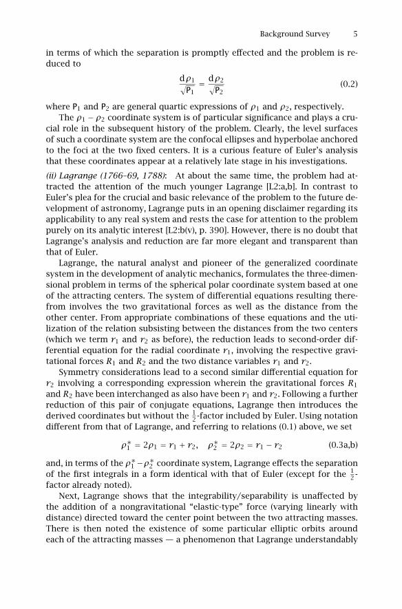
in terms of which the separation is promptly effected and the problem is re-duced to

dρ1√P1= dρ2√

P2(0.2)

where P1 and P2 are general quartic expressions of ρ1 and ρ2, respectively.The ρ1 − ρ2 coordinate system is of particular significance and plays a cru-

cial role in the subsequent history of the problem. Clearly, the level surfacesof such a coordinate system are the confocal ellipses and hyperbolae anchoredto the foci at the two fixed centers. It is a curious feature of Euler’s analysisthat these coordinates appear at a relatively late stage in his investigations.

(ii) Lagrange (1766–69, 1788): At about the same time, the problem had at-tracted the attention of the much younger Lagrange [L2:a,b]. In contrast toEuler’s plea for the crucial and basic relevance of the problem to the future de-velopment of astronomy, Lagrange puts in an opening disclaimer regarding itsapplicability to any real system and rests the case for attention to the problempurely on its analytic interest [L2:b(v), p. 390]. However, there is no doubt thatLagrange’s analysis and reduction are far more elegant and transparent thanthat of Euler.

Lagrange, the natural analyst and pioneer of the generalized coordinatesystem in the development of analytic mechanics, formulates the three-dimen-sional problem in terms of the spherical polar coordinate system based at oneof the attracting centers. The system of differential equations resulting there-from involves the two gravitational forces as well as the distance from theother center. From appropriate combinations of these equations and the uti-lization of the relation subsisting between the distances from the two centers(which we term r1 and r2 as before), the reduction leads to second-order dif-ferential equation for the radial coordinate r1, involving the respective gravi-tational forces R1 and R2 and the two distance variables r1 and r2.

Symmetry considerations lead to a second similar differential equation forr2 involving a corresponding expression wherein the gravitational forces R1

and R2 have been interchanged as also have been r1 and r2. Following a furtherreduction of this pair of conjugate equations, Lagrange then introduces thederived coordinates but without the 1

2 -factor included by Euler. Using notationdifferent from that of Lagrange, and referring to relations (0.1) above, we set

ρ∗1 = 2ρ1 = r1 + r2, ρ∗2 = 2ρ2 = r1 − r2 (0.3a,b)

and, in terms of the ρ∗1 −ρ∗2 coordinate system, Lagrange effects the separationof the first integrals in a form identical with that of Euler (except for the 1

2 -factor already noted).

Next, Lagrange shows that the integrability/separability is unaffected bythe addition of a nongravitational “elastic-type” force (varying linearly withdistance) directed toward the center point between the two attracting masses.There is then noted the existence of some particular elliptic orbits aroundeach of the attracting masses — a phenomenon that Lagrange understandably

6 Ch 0 General Introduction

records as “very remarkable” [L2, b(v), p. 397]. There follows a discussion ofsome “time of traverse” features of particular orbits in relation to some generalresults of Lambert [L1].

Lagrange’s derivation is remarkable for its clarity and the general eleganceof its presentation. We record verbatim some of Lagrange’s concluding re-marks in his treatment of the Euler problem, from the English translation byBoissonade and Vagliente [L2, b(v), p. 400] of the second edition [L2, b(ii)].

The problem which we just solved was first solved by Euler for the case wherethere are only two fixed centers which attract inversely proportional to thesquare of the distances and where the body moves in plane containing thetwo centers (Memoires de Berlin for 1760). His solution is specifically remark-able for the skill he has shown in using various substitutions to reduce thedifferential equations to the first order and to integration. These differentialequations could not be solved by known methods because of their complexity.

By giving a different form to these equations, I obtained directly the sameresults and I was even able to generalize them to the case where the curve isnot in the same plane and where there is also a force proportional to the dis-tance and directed toward a fixed center located in the middle of the two othercenters. The reader should refer to the Fourth Volume of the old Memoires deTurin, from which the preceding analysis is taken and in which the case isfound where one of the centers is moving toward infinity and the force di-rected toward this center becomes uniform and acts along parallel lines. Itis surprising that in this case the solution is not greatly simplified. Only theradicals, which enter in the denominators of the individual equations, containonly the third degree of these variables rather than the fourth degree, whichalso makes their integration dependent on the rectification of conic sections.

This latter modification of the physical problem might even find an application(the Stark effect), a century after Lagrange had written his last word.

(iii) The Coordinate System: Before we close our survey of the eighteenth cen-tury, it is appropriate to add a further comment on the coordinate system.

The coordinate system (r1, r2), on which Lagrange based his formulationand which Euler had eventually recognized as a basis for his “methodus suc-cinctior” leading to separation, may by its nature be termed the bipolar coor-dinate system. Both of the derived systems (ρ1, ρ2) and (ρ∗1 , ρ

∗2 ) are elliptic

coordinate systems: these two systems are identical except for the 12 -factor,

and we shall confine our attention to the (ρ1, ρ2) system. We shall refer to thissystem as the Euler–Lagrange elliptic coordinate system or more frequently asthe EL elliptic coordinate system.

This coordinate system plays a central role in the subsequent history of theproblem. It is not surprising that this should be so, as this system — or somesimple variant thereof — is necessary to facilitate separation. However, theaccepted centrality of its role in effecting the transition to the first integralsmay also have precluded the possibility of effecting the second integration toyield a general solution. This is an issue to which we shall return.

Background Survey 7

The Nineteenth Century

(i) Lagrange/Legendre: With the appearance of Lagrange’s landmark work Me-chanique Analytique in 1788, the problem and its analysis received a muchwider exposure. In the subsequent years, Lagrange devoted a good deal of histime and attention to the revision and expansion of his magnum opus for asecond edition. This was prepared in two volumes — the first issued in 1811and the second, which contained the work on dynamics, appeared in print afew weeks after the author’s death in 1815.

Meantime, the problem had attracted the attention of Legendre, who hadindependently observed and commented on the existence of elliptic orbitsabout each of the primaries — the “very remarkable” phenomenon noted byLagrange. These and other observations were recorded by Legendre in his re-spective treatises on calculus and elliptic functions [L3, (a) and (b)]. A genera-tion later, these curious orbits would be recognized as particular cases of theconsequences of what became known as Bonnet’s theorem [B3].

(ii) Jacobi: The next milestone in the history of the Euler problem is markedby the investigations of Jacobi, as recorded in his lecture course at the Univer-sity of Konigsberg. Following the appearance of Hamilton’s “General Method”in 1834–35 [H1], Jacobi promptly developed the general procedure for the anal-ysis of dynamical systems through a first-order partial differential equation,since known as the Hamilton–Jacobi equation and procedure. He demonstratedthe method in his lecture courses. The lectures he delivered at Konigsberg in1842–43 were recorded by C.W. Borchardt and were published, under the edi-torship of A. Clebsch, over two decades later in 1866 [J1].

In his analysis of the Euler problem, Jacobi takes as his framework the bipo-lar coordinate system as laid out by Lagrange and formulates the Hamilton–Jacobi equation for the problem in these coordinates. Then transforming to theEL coordinate system, he is led to the separated form of the Hamilton–Jacobidifferential equation (lecture 25).

Motivated by the larger context of dynamical systems, extending beyondthe confines of celestial mechanics, Jacobi is led to investigate the separationissue. In the absence of any general method, he must pursue a partially inverseprocedure — “on finding a remarkable substitution, look for the problems towhich it can be applied.” In the next three lectures (26–28), he introduces anddevelops a general system of coordinates, since known as Jacobi’s ellipsoidalcoordinates, and points out their applicability to a number of identified prob-lems. Specifically, he frames the scheme to investigate the motion of a particleon a general ellipsoid in Rn.

Having noted the particular form taken by Jacobi’s ellipsoidal coordinatesin two- and three-dimensional Euclidean space, he then returns to the Eulerproblem (lecture 29). The planar form of Jacobi’s elliptic coordinates, denotedby (λ1, λ1), is related to the EL elliptic coordinates (ρ1, ρ2) as follows:

12(r1 + r2) = ρ1 =

√a+ λ1, 1

2(r1 − r2) = ρ2 =√a+ λ2 (0.4a,b)

8 Ch 0 General Introduction

where a is the length parameter of the Jacobi system. He then demonstratesthe separability of the Hamilton–Jacobi partial differential equation for theEuler problem in the (slightly more general) Jacobi elliptic coordinate system,before finally reverting to the EL elliptic coordinate system for the expressionof the first integrals.

(iii) Liouville: Influenced by the ideas of Jacobi, Liouville recognized the rel-evance of the essential concepts to the utilization of general orthogonal co-ordinates in the exploration of geodesics on the general triaxial ellipsoid [L6,a]. In line with that analysis, he investigated the parallel applicability to theLagrangian formulation of dynamical systems. The crucial feature was separa-bility, and it led to his formulation of sufficient conditions for separability ofdynamical systems in general orthogonal coordinates [L6, b].

Liouville noted that most of the known integrable problems met his condi-tions for separability. In particular, he focused on the applicability to the Eulerproblem, including the problem as extended by Lagrange, and cited the use ofJacobi’s ellipsoidal coordinates. Moreover, in the planar case, he showed thatit admitted the additional modification by permitting the inclusion of an addi-tional attractive force, normal to the axis defined by the two centers, and pro-portional to the inverse of the cube of the distance therefrom. He also raisesthe question of allowing the two primaries to rotate [L6, a(ii), pp. 440–1].

The attention of Jacobi and especially that of Liouville were crucial in main-taining interest in the problem, and many of the investigations in the latterhalf of the century reflect back to them. Liouville was probably the most influ-ential mathematician of his time, and we shall see that in the ensuing years,many of the points of note are linked to his former students and associates —cf. Lutzen [L8].

A curious feature of their work is that neither Jacobi nor Liouville made anymove toward the second integration for a complete solution; we shall returnto this point later.

(iv) J.A. Serret, J.L.F. Bertrand, J.G. Darboux: Also in the 1840s, Lagrange’swork had attracted the attention of the young Joseph Alfred Serret1 — a stu-dent of Liouville. In his thesis, presented at the Faculty of Sciences at Paris,he pointed out that part of Lagrange’s analysis of the Euler problem neededsome clarification and amplification in order to give a rigorous treatment anda satisfactory derivation of the results: cf. [L2, b(v), note 26, p. 590].

During the same decade, when decisions were being made for a third edi-tion of Lagrange’s Mecanique Analytique, the one chosen as editor was JosephBertrand — another protege of Liouville. Bertrand prepared a significantly ex-panded edition with copious notes on the more recent developments — specifi-cally, the Hamilton–Jacobi theory as well as the results of Poisson and Liouville.In the discussion of the Euler problem, Bertrand included the above-mentionedmodifications and clarifications of J.A. Serret. The third edition, in two vol-umes, was published in Paris in the years 1852–55.

1 Joseph Alfred Serret and Paul Serret, previously cited [S1], were brothers.

Background Survey 9

As already noted, the lectures of Jacobi appeared in print in Berlin in 1866.Later the complete works of Jacobi were prepared under the general editorshipof E. Lettner. These were published in Berlin in 1884; they included a reissueof the Konigsberg lectures with a foreword by K.T. Weierstrass.

Meanwhile, the publication of the complete works of Lagrange was under-taken by Le Ministere de l’Instruction Publique, with Gauthier-Villars (Paris) asImprimeur-Libraire. The project (Oeuvres de Lagrange) comprised 14 volumesthat appeared over the years 1867–92. The general editor was J.A. Serret who,by the time of his death in 1885, had prepared volumes I–X and seen themthrough to publication. Volumes XI and XII constitute the fourth edition ofMecanique Analytique under the editorship of Jean Gaston Darboux, and thesemade their appearance in the anniversary year 1888. The final two volumes,which deal with the correspondence of Lagrange, were edited by L. Lafauneand appeared in 1892.

It would seem that these publications may have led to a revival of inter-est in the works of Liouville. In particular, there appeared the investigationsof Stackel on separability in 1890 and 1891 [S5] and the subsequent workof Levi-Civita [L4] in 1904. In Stackel’s analysis, it is shown that for generalorthogonal coordinates, Liouville’s requirements for separability are both nec-essary and sufficient, while (independently) Levi-Civita has shown that if thepotential depends on all coordinates, then for the system to be separable thesecoordinates must be orthogonal. The term “Liouvillian” has since been appliedto many systems satisfying “Liouville’s conditions” in a variety of forms morerestrictive than that of Liouville’s general formulation [L8, pp. 704–5].

In 1889 appeared the work of Velde [V3], which is a reconsideration of aform of the generalization of the Euler problem as formulated by Liouville.More significant is the analysis of Darboux [D1], which appeared in 1901.Therein it is shown that separability, in the EL elliptic coordinate system,persists for the Euler problem if there are added two further complex-valuedmasses that are conjugates of each other and situated respectively at the imag-inary foci of the elliptic coordinate system. This extension has relevance to theVinti problem to be discussed presently.

For celestial mechanics, the end of the century is marked by the massiveinvestigations of Poincare [P3]; however, there is no indication that the Eulerproblem held any interest for him.

The Twentieth Century — and Later

(i) Charlier, Hiltebeitel, Plummer : The opening decade of the twentieth cen-tury brought the two-volume treatise on celestial mechanics by Charlier [C1],the volumes appearing respectively in 1902 and 1907. The first volume is de-voted to analysis while the second is concerned with specific problems in as-tronomy. In volume one, there is a thorough investigation of the Euler prob-lem — the first such thorough treatment since that given in the lectures ofJacobi [J1] a half-century earlier.

10 Ch 0 General Introduction

It is worth paying particular attention to the layout of Charlier’s first vol-ume. Following the introduction of Lagrangian mechanics and the separabilitytheorem of Liouville, Charlier immediately cites the Euler problem in EL ellipticcoordinates as an example for the applicability of the latter theorem of Liou-ville — all in the first chapter. The second chapter introduces the Hamilton–Jacobi procedure and, following the determination of the separability criterionand the citation of Stackel’s theorem, moves to an investigation of periodicsolutions. The third chapter is devoted entirely to the Euler problem for thevarious ranges (negative, zero, and positive) of the energy constant. Here theanalysis is particularly focused on the possible ranges for the zeros of therelevant quartics appearing in the elliptic integrals. Examples are cited andsamples of typical orbits for specific ranges are illustrated. Not until chapterfour is the two-body (Kepler) problem discussed. This is followed in chapterfive by an analysis of the three-body problem. The later chapters six and sevendeal with perturbation theory.

Thus, in Charlier’s presentation, the Euler problem has priority and takescenter stage, with the Kepler problem taking a secondary role as the degener-ate case. The significance of this unique feature of Charlier’s approach doesnot seem to have drawn much comment.

A few years later in 1911, the paper by Hiltebeitel [H4] includes a detaileddiscussion of the Euler problem and its generalizations. Therein may be foundthe general formulation where the cases treated by Darboux, Liouville, La-grange, and Euler can be seen in the context of the general problem, each oneof those mentioned being a particular case of the preceding one. The analysisfollows Charlier in its concentration on the ranges for the roots of the relevantquartics; again examples are cited and some typical orbits are illustrated.

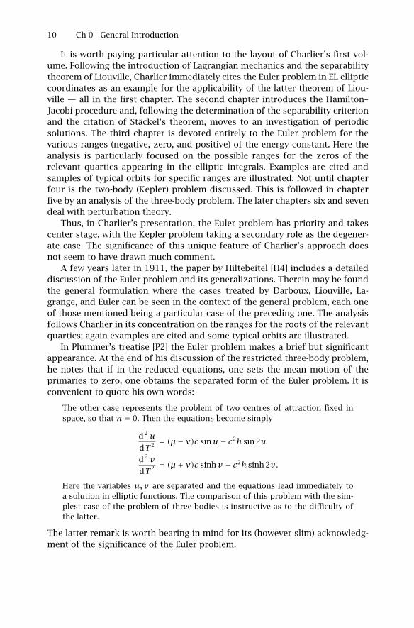
In Plummer’s treatise [P2] the Euler problem makes a brief but significantappearance. At the end of his discussion of the restricted three-body problem,he notes that if in the reduced equations, one sets the mean motion of theprimaries to zero, one obtains the separated form of the Euler problem. It isconvenient to quote his own words:

The other case represents the problem of two centres of attraction fixed inspace, so that n = 0. Then the equations become simply

d2udT 2 = (μ − ν)c sinu− c2h sin 2u

d2 vdT 2 = (μ + ν)c sinhv − c2h sinh 2v.

Here the variables u,v are separated and the equations lead immediately toa solution in elliptic functions. The comparison of this problem with the sim-plest case of the problem of three bodies is instructive as to the difficulty ofthe latter.

The latter remark is worth bearing in mind for its (however slim) acknowledg-ment of the significance of the Euler problem.

Background Survey 11

The comment that the separated equations “lead immediately to a solutionin elliptic functions” is typical of what is generally said — if anything at allis said — by the several authors at this point where separation of the firstintegrals has been achieved. In the various textbooks issued throughout thetwentieth century, the reader is told that the solution of the Euler problemis expressible in terms of elliptic functions, without any specification of whattype of elliptic function or any indication of how such a form is to be attained.As will be noted presently, there is one textbook that at least partially breaksthis pattern in that it identifies the functions as those of Jacobi — but withoutany indication of how this is to be done; and that text appears in the twenty-first century [C3].

(ii) The Quantum Connection — and Some Corrections: Returning to the chro-nology, in the 1920s the Euler problem received attention from another quar-ter. Within a decade of the appearance of Bohr’s quantum theory, the molecu-lar analog of the Euler problem was being explored by two young students. Thequantum problem is that of the hydrogen molecule ion H+2 and the studentswere K.F. Niessen [N1, 1923] at Utrecht and W. Pauli [P1, 1922] at Munich. InPauli’s work, the EL elliptic coordinates are normalized with the separationparameter. In both cases, the authors rely on the lectures of Jacobi and onCharlier’s treatise; the several types of orbit are classified and energy calcula-tions are made for particular orbits. Their work was noted by Sommerfeld inthe fourth edition of his Atombau und Spectralinien (1924) and also in Born’sVorlesungen uber Atommechanik (1925), where the discrepancies between en-ergy calculations and the measured values are noted. Further work was doneby Teller, Burrau, Richardson, and others. We shall not attempt to do justice tothis story; it is ably told in the biography of Pauli by Charles Enz [E1, pp. 63–70]. Therein it is noted that the H+2 problem is both “the simplest molecularproblem” and also the most complicated problem that the old quantum theorycould handle.

Shortly thereafter, in the USSR it was observed that there were some inac-curacies in Charlier’s analysis of the Euler problem. This appeared in the 1927paper of Tallquist [T1] who besides making the appropriate corrections in thework of Charlier also refined the classification of the orbits. This correctionand refinement was further extended in the following decade in the work ofBadalyan [B1, 1934].

(iii) Prange, Whittaker, Wintner : The general issue of integration proceduresin analytic mechanics was fully surveyed in the comprehensive article pre-pared by Prange for the Encyclopedia of Mathematical Sciences appearing in1933 [P4]. Also there appeared the textbooks of Whittaker and Wintner, re-spectively. The first edition of Whittaker’s treatise appeared in 1904, with latereditions in 1917, 1927, and 1937; a German translation appeared in 1924. Histreatment of the Euler problem is brief: having reduced the problem to thefirst integrals, he mentions that “the solution can be expressed in terms of el-liptic functions” [W2, iv: p. 99]. In the book by Wintner (1947) [W3, pp. 145–7],

12 Ch 0 General Introduction

following a formulation in terms of bipolar coordinates, the separation is ef-fected by transforming to EL elliptic coordinates; some qualitative features ofthe motion are mentioned.

(iv) 1950–2000: In the second half of the century, the major analytic advancewas initiated by Kolmogorov [K1, a,b], particularly in his celebrated 1954 ICMaddress [K1, (b)], an English translation of which appears in Appendix D ofreference [A1].

In that 1954 address, Kolmogorov set out the structure of his approach inthe context of the classical integrable problems. In citing the Euler problem,he notes that

the extremely instructive qualitative analysis of the problem on the attractionby two immovable centers that was made in Charlier’s well-known treatise hasproven to be incomplete and partially erroneous. It has been twice corrected[by Tallquist and Badalyan].

[A1, Appendix D; p. 269, footnote]

He then goes on to emphasize that

the real significance for Classical Mechanics of the analysis that I have made ofDynamical Systems on T 2 depends on whether there are sufficiently importantexamples of canonical systems with two degrees of freedom that cannot beintegrated by classical methods and in which invariant (with respect to thetransformation St) two-dimensional tori play a significant role.

[A1, Appendix D; p. 270]

The strength of his approach will reveal itself in the nonintegrable case. Thisled to the major results of Arnold and Moser and what became known as theKAM theory, recorded in the book by Abraham and Marsden (1967) [A1]. TheKAM theory is detailed in the textbook of Siegel•Moser (1971) [S2], and also inthat of Arnold, Kozlov, and Neishtadt (1985; 1993; 1997) [A8]. As previouslynoted, the KAM theory is also discussed in the survey “Celestial Encounters”(1996) [D1].

This may be an appropriate point to note that the first English translationof the Mecanique Analytique of Lagrange appeared in 1996 [L2, b(v)].

Meantime, the previously noted idea of Paul Serret [S1] in generalizing thecontext of the Kepler problem to a space of constant curvature was taken upand applied to the Euler problem by Alekseev (1965) [A4], which led to furtherexploration in that area, mainly within the USSR. The recent developments inthis area, together with an account of the work over the intervening years, maybe found in the book devoted to the topic by Vozmischeva (2003) [V5].

The advent of the space age in the 1950s with the consequent new interestin space dynamics stimulated the quest for specific solutions and led to arenewal of interest in the Euler problem. There were investigations in two areas— an examination of specific cases of the Euler problem and an investigation ofthe potential use of solutions of the Euler problem as a basis of approximationfor solutions of the restricted three-body problem. In the former, we mentionespecially the work of Deprit (1962) [D2]; and in the latter where the solution

Background Survey 13

of the Euler problem is to be used as an “intermediate orbit,” we note the workof Arenstorf and Davidson (1963) [A7]. Considerable further work on theselines is surveyed in the book by Szebehely (1967) [S8], which is particularlyinformative especially in the notes and reference lists at the close of Chapters3 and 10.

The Euler problem gets mention in the book by Arnold (1974) [A8] and getsbrief coverage in the book by Arnold, Kozlov, and Neishtadt (1985) [A9], wherethere is strong emphasis on according due recognition to the achievement ofJacobi [A9, p. 128].

(v) The Quantum Connection Revisited: Following the appearance of Wave Me-chanics in the latter half of the 1920s, interest in the classical approach tothe hydrogen ion, as a basis for “semiclassical” quantization, seems to havewaned. After the lapse of one-half century, there appeared the curiously inter-esting — and somewhat baffling — work of Strand and Reinhardt (1979) [S7].2

Therein the problem is normalized by the separation length (b) and formu-lated in terms of the EL coordinate system — also normalized by b.3 We shallpresently discuss the limitations inherent in such a formulation. Here we con-fine ourselves to the results presented in [S7].

The features of the work we wish to note are twofold:

1. the formulation incorporates the introduction of the regularizing transfor-mation;

2. the solutions are presented in terms of Jacobian elliptic functions.

Following a discussion of the accessible/nonaccessible regions based on ananalysis of the quartics, the solution forms are then presented in terms ofJacobian elliptic functions with the modulus expressed in terms of the rootsof the quartics. The solution forms for ρ2/b are given in relations (2.17) whilethose for ρ1/b are given in relations (2.18).

Relation (2.17a) as it stands is baffling and defies any attempt to see howit could arise; however, if it is taken that in that equation the symbol dn is amisprint for what should read sn, then the two relations (2.17a,b) by appropri-ate rescaling can be brought into conformity with the solution forms for thecase β = 0, presented in the present work, namely, relation (6.9) and (6.13) ofSection 6, Chapter 3.

Relations (2.18) for ρ1/b present other problems. The form (2.18b) givenfor the case where two complex roots arise appears simpler than the form(2.18a) given for the case of four real roots. Complex roots do not arise inthe planar case; in the analysis presented here, it is shown how the generalcase can be reduced to the planar case (Chapter 4). If complex roots arise, itis not clear how they give rise to a solution, simpler in form to that of theplanar case. Accordingly, it is not obvious what is the realm of relevance of the

2 This work has been brought to my attention by Professor A.J. Bracken of the University ofQueensland, which I gratefully acknowledge.

3 The authors use the symbol c for the separation length; for consistency with the notation ofthe present work, we use the symbol b.

14 Ch 0 General Introduction

solution form (2.18b). We concentrate therefore on the solution form (2.18a)for the case where all four roots are real. Without giving any indication howsuch a solution form could arise, the solution is presented as a quotient oflinear functions of the factor sn2 as a function of the half-argument; if onenotes that

sn2 12u =

1− cnu1+ dnu

then clearly the solution form (2.18a) can be expressed as a quotient of lin-ear functions of the elliptic functions cn and dn of the full argument. Withthe appropriate rescaling of all the quantities involved, this solution could bebrought into conformity with the solution forms given in Chapter 3, e.g., rela-tion (9.29) of Section 9 or (9A.33) of Section 9A, depending on the identity ofξ2 and ξ3. However, the form in which the solution (2.18a) in [S7] is expressedhas the negative feature that in the Kepler limit as b tends to zero, two of theroots tend to infinity as does also the left side ξ = ρ1/b. It is regrettable thatthis work has been left in such an unattractive form — at least partly from thechoice of coordinate system and normalization procedure; further comment isnot possible without a clearer indication of how the solution was arrived at.

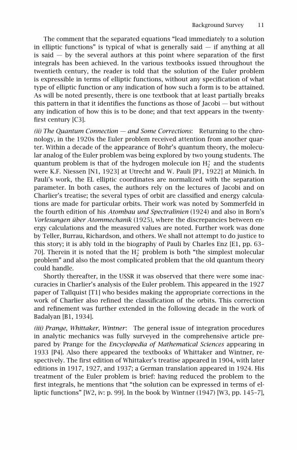
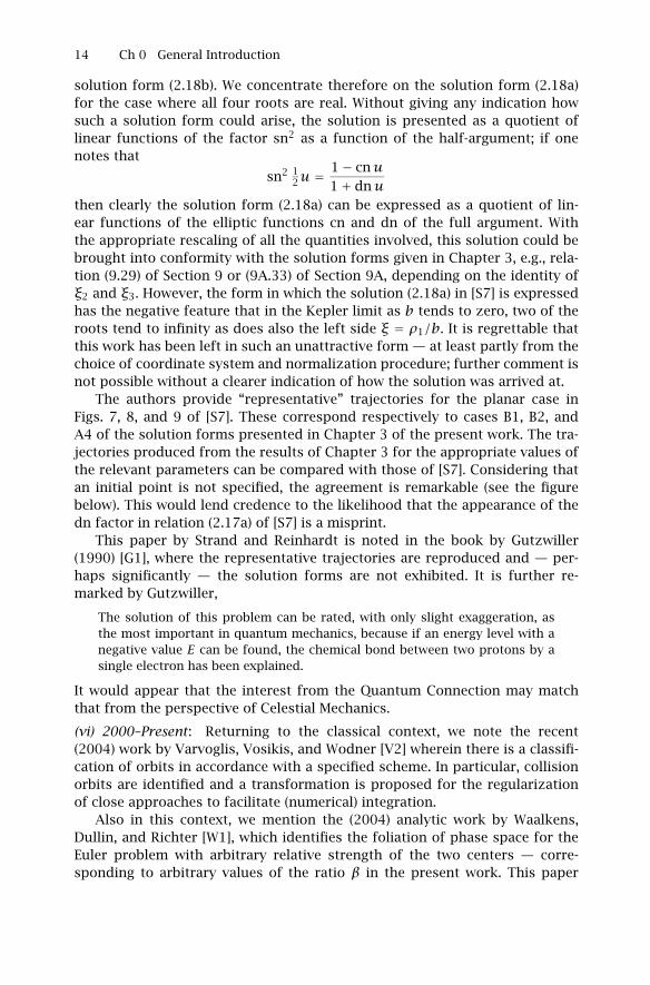
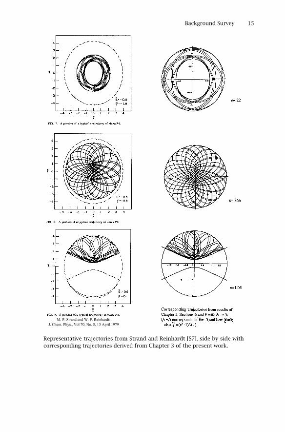
The authors provide “representative” trajectories for the planar case inFigs. 7, 8, and 9 of [S7]. These correspond respectively to cases B1, B2, andA4 of the solution forms presented in Chapter 3 of the present work. The tra-jectories produced from the results of Chapter 3 for the appropriate values ofthe relevant parameters can be compared with those of [S7]. Considering thatan initial point is not specified, the agreement is remarkable (see the figurebelow). This would lend credence to the likelihood that the appearance of thedn factor in relation (2.17a) of [S7] is a misprint.

This paper by Strand and Reinhardt is noted in the book by Gutzwiller(1990) [G1], where the representative trajectories are reproduced and — per-haps significantly — the solution forms are not exhibited. It is further re-marked by Gutzwiller,

The solution of this problem can be rated, with only slight exaggeration, asthe most important in quantum mechanics, because if an energy level with anegative value E can be found, the chemical bond between two protons by asingle electron has been explained.

It would appear that the interest from the Quantum Connection may matchthat from the perspective of Celestial Mechanics.

(vi) 2000–Present: Returning to the classical context, we note the recent(2004) work by Varvoglis, Vosikis, and Wodner [V2] wherein there is a classifi-cation of orbits in accordance with a specified scheme. In particular, collisionorbits are identified and a transformation is proposed for the regularizationof close approaches to facilitate (numerical) integration.

Also in this context, we mention the (2004) analytic work by Waalkens,Dullin, and Richter [W1], which identifies the foliation of phase space for theEuler problem with arbitrary relative strength of the two centers — corre-sponding to arbitrary values of the ratio β in the present work. This paper

Background Survey 15

Representative trajectories from Strand and Reinhardt [S7], side by side withcorresponding trajectories derived from Chapter 3 of the present work.

M. P. Strand and W. P. Reinhardt:J. Chem. Phys., Vol 70, No. 8, 15 April 1979