proj car prices
TRANSCRIPT

7/29/2019 proj Car Prices
http://slidepdf.com/reader/full/proj-car-prices 1/14
Car Price Analysis of Mitsubishi
Section 1. Purpose of the researchPresently, people’s income and car price are two main problems which affecting car sales.
Although economy of the whole world is not really good at this time, the quality and property of cars are still getting better since the improvement of technology. In this article, we would
investigate the factors of buying cars which consumers really concern, and analysis that is there any
obviously relation between pricing factors and properities of cars.
Section 2. Methods of the researchI would use SAS program for our regressing module, and choose 4 kinds of cars from Mitsubishi.
These 4 kinds of cars are 4-doors vehicle, van, import, and business. Since the kinds of these cars
are too complicated, we just select the kinds whose price is under US$33,000. Next I decide 5
variables in my regression module which are horsepower(ps/rpm), Torpque (kg-m/rpm),
Displacement(cc), length of axle(mm), and weight of empty car(kg). The original regression
module is as following:
55443322110X X X X X Y β β β β β β +++++=
The definition of variables are as following:
Y = Car Price
1 X = horsepower
2 X = Torque
3 X = Displacement
4 X = Length of axle
5 X = weight of empty car
Section 3. Research Process
Purpose of research
7/29/2019 proj Car Prices
http://slidepdf.com/reader/full/proj-car-prices 2/14
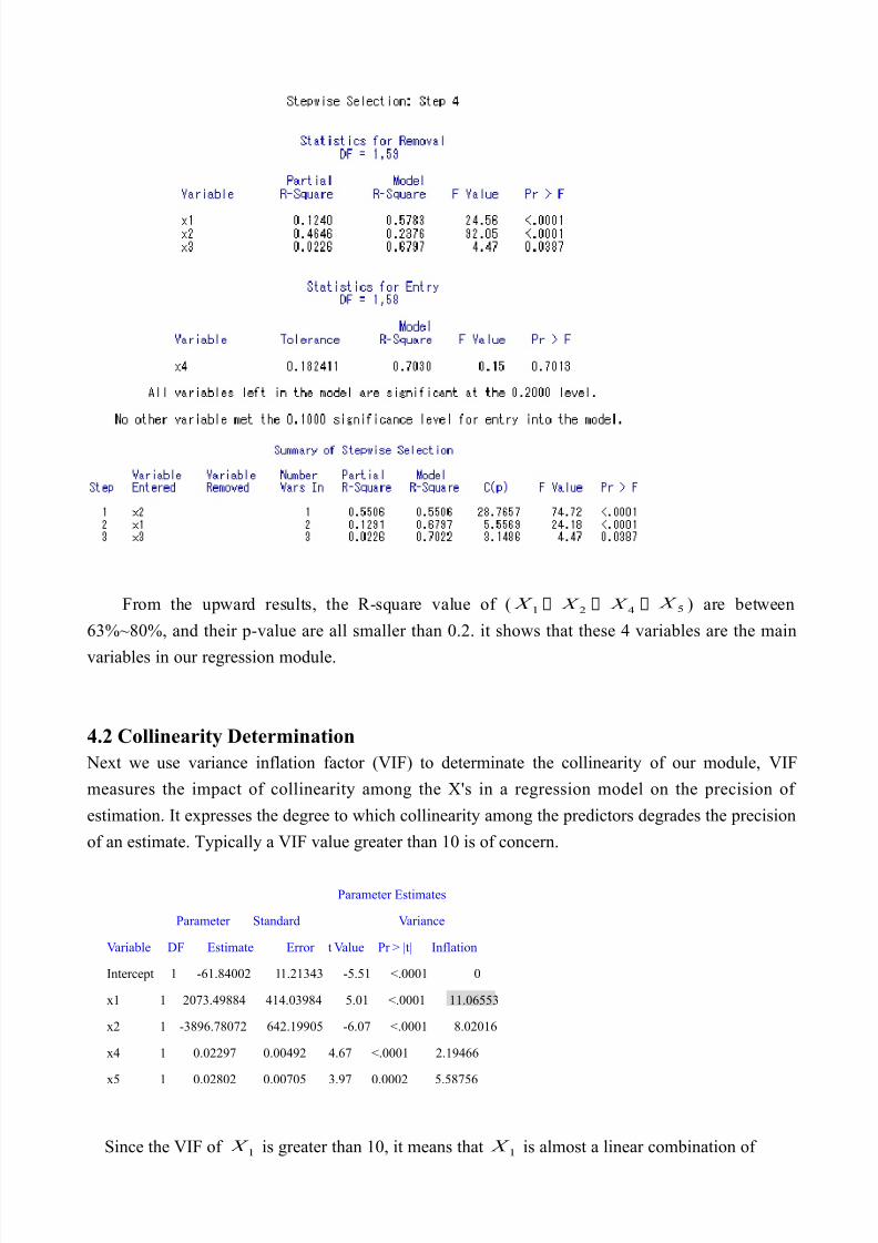
Section 4. Analysis and Results4.1 Building regression module
Using the collected data and analyzing by SAS system, I got the following results:
The SAS System
Statistics for Removal
DF = 1,67
Partial Model
Variable R-Square R-Square F Value Pr > F
x1 0.0742 0.7277 25.08 <.0001
x2 0.1089 0.6929 36.82 <.0001
x4 0.0645 0.7373 21.82 <.0001
x5 0.0467 0.7551 15.80 0.0002
Statistics for Entry
DF = 1,66
Model
Variable Tolerance R-Square F Value Pr > F
x3 0.068111 0.8066 1.61 0.2085
All variables left in the model are significant at the 0.2000 level.
No other variable met the 0.1000 significance level for entry into the model.
Summary of Stepwise Selection
Variable Variable Number Partial Model
Step Entered Removed Vars In R-Square R-Square C(p) F Value Pr > F
1 x5 1 0.6335 0.6335 57.0515 121.00 <.0001
2 x4 2 0.0567 0.6902 39.7047 12.63 0.0007
3 x2 3 0.0375 0.7277 28.9229 9.35 0.0032
4 x1 4 0.0742 0.8018 5.6135 25.08 <.0001
Methods of research
Analysis and Results
Conclusion
7/29/2019 proj Car Prices
http://slidepdf.com/reader/full/proj-car-prices 3/14
From the upward results, the R-square value of ( 1 X : 2
X : 4 X : 5
X ) are between
63%~80%, and their p-value are all smaller than 0.2. it shows that these 4 variables are the main
variables in our regression module.
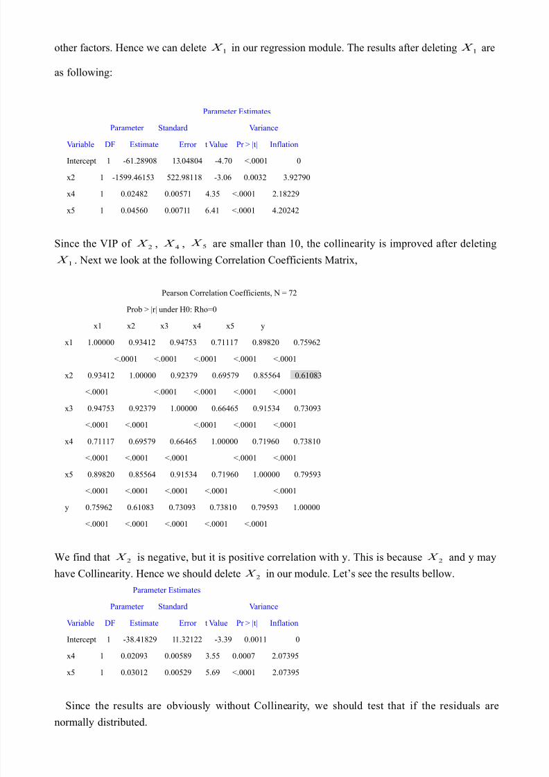
4.2 Collinearity Determination
Next we use variance inflation factor (VIF) to determinate the collinearity of our module, VIF
measures the impact of collinearity among the X's in a regression model on the precision of
estimation. It expresses the degree to which collinearity among the predictors degrades the precision
of an estimate. Typically a VIF value greater than 10 is of concern.
Parameter Estimates
Parameter Standard Variance
Variable DF Estimate Error t Value Pr > |t| Inflation
Intercept 1 -61.84002 11.21343 -5.51 <.0001 0
x1 1 2073.49884 414.03984 5.01 <.0001 11.06553
x2 1 -3896.78072 642.19905 -6.07 <.0001 8.02016
x4 1 0.02297 0.00492 4.67 <.0001 2.19466
x5 1 0.02802 0.00705 3.97 0.0002 5.58756
Since the VIF of 1 X is greater than 10, it means that 1
X is almost a linear combination of
7/29/2019 proj Car Prices
http://slidepdf.com/reader/full/proj-car-prices 4/14
other factors. Hence we can delete 1 X in our regression module. The results after deleting 1
X are
as following:
Parameter Estimates
Parameter Standard Variance
Variable DF Estimate Error t Value Pr > |t| Inflation
Intercept 1 -61.28908 13.04804 -4.70 <.0001 0
x2 1 -1599.46153 522.98118 -3.06 0.0032 3.92790
x4 1 0.02482 0.00571 4.35 <.0001 2.18229
x5 1 0.04560 0.00711 6.41 <.0001 4.20242
Since the VIP of 2 X , 4
X , 5 X are smaller than 10, the collinearity is improved after deleting
1 X . Next we look at the following Correlation Coefficients Matrix,
Pearson Correlation Coefficients, N = 72
Prob > |r| under H0: Rho=0
x1 x2 x3 x4 x5 y
x1 1.00000 0.93412 0.94753 0.71117 0.89820 0.75962
<.0001 <.0001 <.0001 <.0001 <.0001
x2 0.93412 1.00000 0.92379 0.69579 0.85564 0.61083
<.0001 <.0001 <.0001 <.0001 <.0001
x3 0.94753 0.92379 1.00000 0.66465 0.91534 0.73093
<.0001 <.0001 <.0001 <.0001 <.0001
x4 0.71117 0.69579 0.66465 1.00000 0.71960 0.73810
<.0001 <.0001 <.0001 <.0001 <.0001
x5 0.89820 0.85564 0.91534 0.71960 1.00000 0.79593
<.0001 <.0001 <.0001 <.0001 <.0001
y 0.75962 0.61083 0.73093 0.73810 0.79593 1.00000
<.0001 <.0001 <.0001 <.0001 <.0001
We find that 2 X is negative, but it is positive correlation with y. This is because 2
X and y may
have Collinearity. Hence we should delete 2 X in our module. Let’s see the results bellow.
Parameter Estimates
Parameter Standard Variance
Variable DF Estimate Error t Value Pr > |t| Inflation
Intercept 1 -38.41829 11.32122 -3.39 0.0011 0
x4 1 0.02093 0.00589 3.55 0.0007 2.07395
x5 1 0.03012 0.00529 5.69 <.0001 2.07395
Since the results are obviously without Collinearity, we should test that if the residuals are
normally distributed.
7/29/2019 proj Car Prices
http://slidepdf.com/reader/full/proj-car-prices 5/14
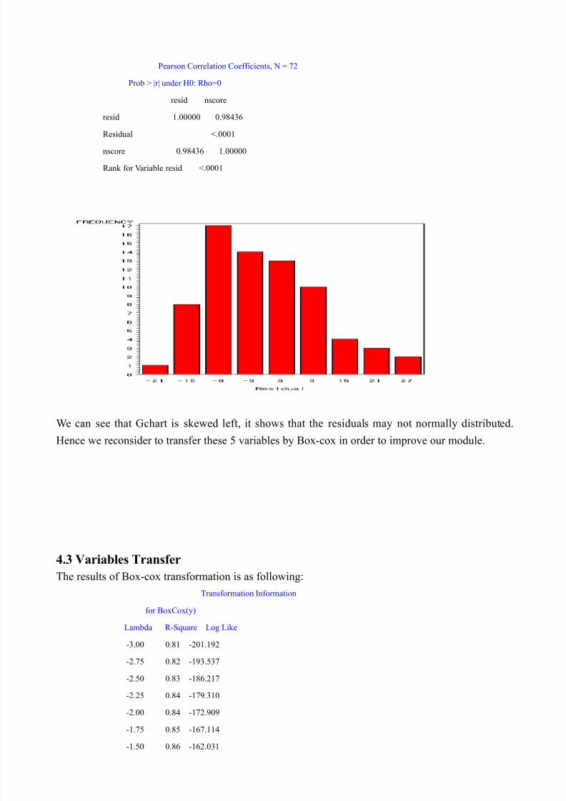
Pearson Correlation Coefficients, N = 72
Prob > |r| under H0: Rho=0
resid nscore
resid 1.00000 0.98436
Residual <.0001
nscore 0.98436 1.00000
Rank for Variable resid <.0001
We can see that Gchart is skewed left, it shows that the residuals may not normally distributed.
Hence we reconsider to transfer these 5 variables by Box-cox in order to improve our module.
4.3 Variables TransferThe results of Box-cox transformation is as following:
Transformation Information
for BoxCox(y)
Lambda R-Square Log Like
-3.00 0.81 -201.192
-2.75 0.82 -193.537
-2.50 0.83 -186.217
-2.25 0.84 -179.310
-2.00 0.84 -172.909
-1.75 0.85 -167.114
-1.50 0.86 -162.031
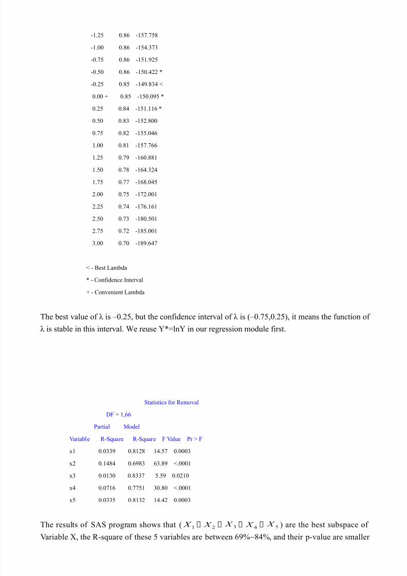
7/29/2019 proj Car Prices
http://slidepdf.com/reader/full/proj-car-prices 6/14
-1.25 0.86 -157.758
-1.00 0.86 -154.373
-0.75 0.86 -151.925
-0.50 0.86 -150.422 *
-0.25 0.85 -149.834 <
0.00 + 0.85 -150.095 *
0.25 0.84 -151.116 *
0.50 0.83 -152.800
0.75 0.82 -155.046
1.00 0.81 -157.766
1.25 0.79 -160.881
1.50 0.78 -164.324
1.75 0.77 -168.045
2.00 0.75 -172.001
2.25 0.74 -176.161
2.50 0.73 -180.501
2.75 0.72 -185.001
3.00 0.70 -189.647
< - Best Lambda
* - Confidence Interval
+ - Convenient Lambda
The best value of λ is –0.25, but the confidence interval of λ is (–0.75,0.25), it means the function of
λ is stable in this interval. We reuse Y*=lnY in our regression module first.
Statistics for Removal
DF = 1,66
Partial Model
Variable R-Square R-Square F Value Pr > F
x1 0.0339 0.8128 14.57 0.0003
x2 0.1484 0.6983 63.89 <.0001
x3 0.0130 0.8337 5.59 0.0210
x4 0.0716 0.7751 30.80 <.0001
x5 0.0335 0.8132 14.42 0.0003
The results of SAS program shows that ( 1 X : 2
X : 3 X : 4
X : 5 X ) are the best subspace of
Variable X, the R-square of these 5 variables are between 69%~84%, and their p-value are smaller
7/29/2019 proj Car Prices
http://slidepdf.com/reader/full/proj-car-prices 7/14
than 0.2, so we use 1 X : 2
X : 3 X : 4
X : 5 X in our module.
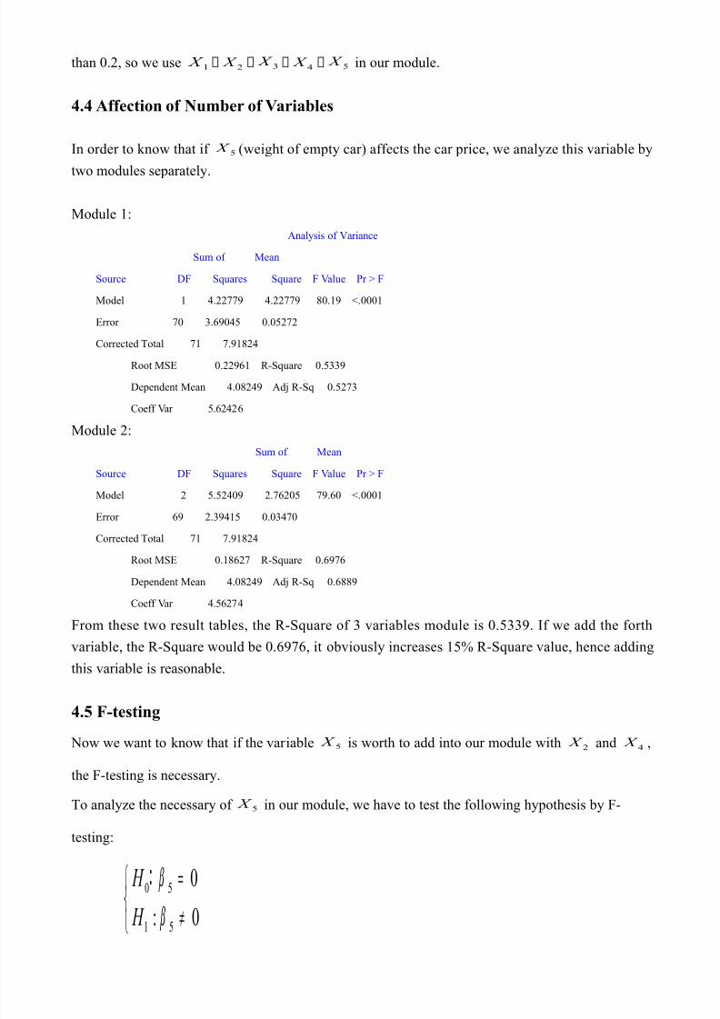
4.4 Affection of Number of Variables
In order to know that if 5 X (weight of empty car) affects the car price, we analyze this variable by
two modules separately.
Module 1:
Analysis of Variance
Sum of Mean
Source DF Squares Square F Value Pr > F
Model 1 4.22779 4.22779 80.19 <.0001
Error 70 3.69045 0.05272
Corrected Total 71 7.91824
Root MSE 0.22961 R-Square 0.5339
Dependent Mean 4.08249 Adj R-Sq 0.5273
Coeff Var 5.62426
Module 2:
Sum of Mean
Source DF Squares Square F Value Pr > F
Model 2 5.52409 2.76205 79.60 <.0001
Error 69 2.39415 0.03470
Corrected Total 71 7.91824
Root MSE 0.18627 R-Square 0.6976
Dependent Mean 4.08249 Adj R-Sq 0.6889
Coeff Var 4.56274
From these two result tables, the R-Square of 3 variables module is 0.5339. If we add the forth
variable, the R-Square would be 0.6976, it obviously increases 15% R-Square value, hence adding
this variable is reasonable.
4.5 F-testing
Now we want to know that if the variable 5 X is worth to add into our module with 2
X and 4 X ,
the F-testing is necessary.
To analyze the necessary of 5 X in our module, we have to test the following hypothesis by F-
testing:
≠
=
0:
0
51
50
β
β
H
: H
7/29/2019 proj Car Prices
http://slidepdf.com/reader/full/proj-car-prices 8/14
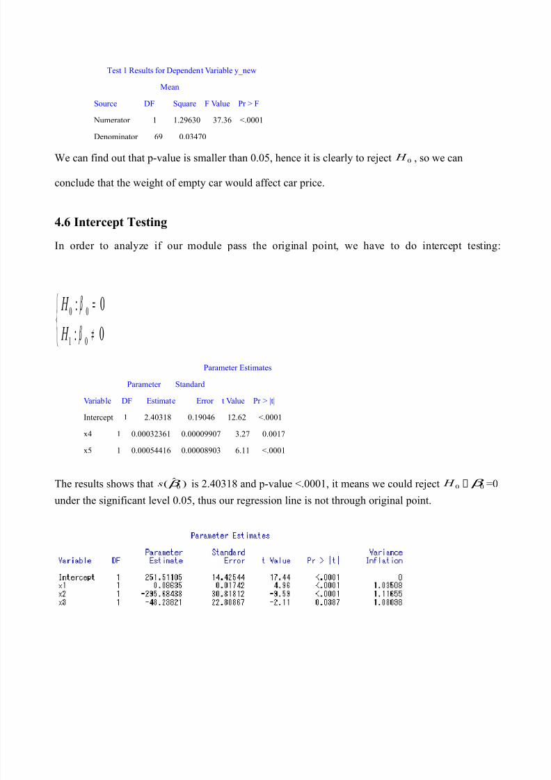
Test 1 Results for Dependent Variable y_new
Mean
Source DF Square F Value Pr > F
Numerator 1 1.29630 37.36 <.0001
Denominator 69 0.03470
We can find out that p-value is smaller than 0.05, hence it is clearly to reject 0 H , so we can
conclude that the weight of empty car would affect car price.
4.6 Intercept Testing
In order to analyze if our module pass the original point, we have to do intercept testing:
≠
=
0:
0:
01
00
β
β
H
H
Parameter Estimates
Parameter Standard
Variable DF Estimate Error t Value Pr > |t|
Intercept 1 2.40318 0.19046 12.62 <.0001
x4 1 0.00032361 0.00009907 3.27 0.0017
x5 1 0.00054416 0.00008903 6.11 <.0001
The results shows that )ˆ(0
β s is 2.40318 and p-value <.0001, it means we could reject 0 H : 0
β =0
under the significant level 0.05, thus our regression line is not through original point.
7/29/2019 proj Car Prices
http://slidepdf.com/reader/full/proj-car-prices 9/14
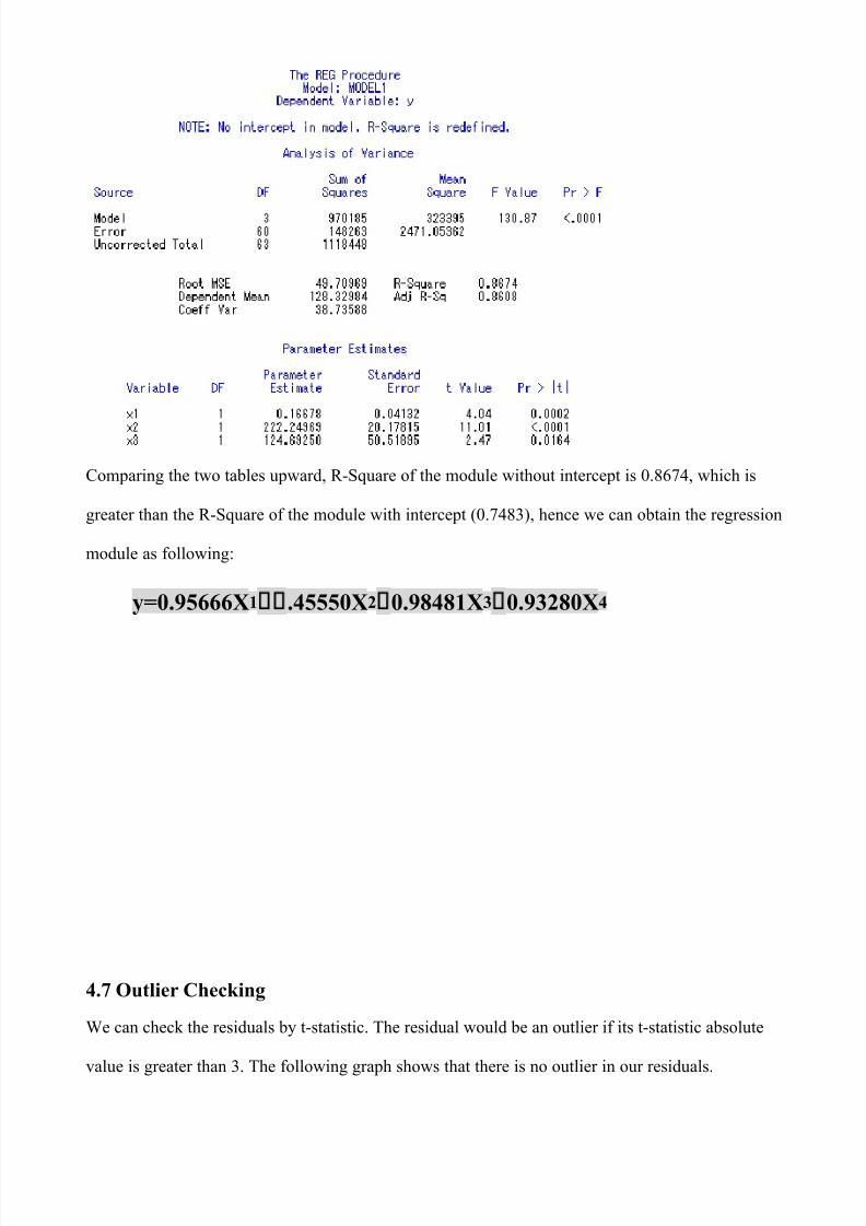
Comparing the two tables upward, R-Square of the module without intercept is 0.8674, which is
greater than the R-Square of the module with intercept (0.7483), hence we can obtain the regression
module as following:
y=0.95666X1::.45550X2:0.98481X3:0.93280X4
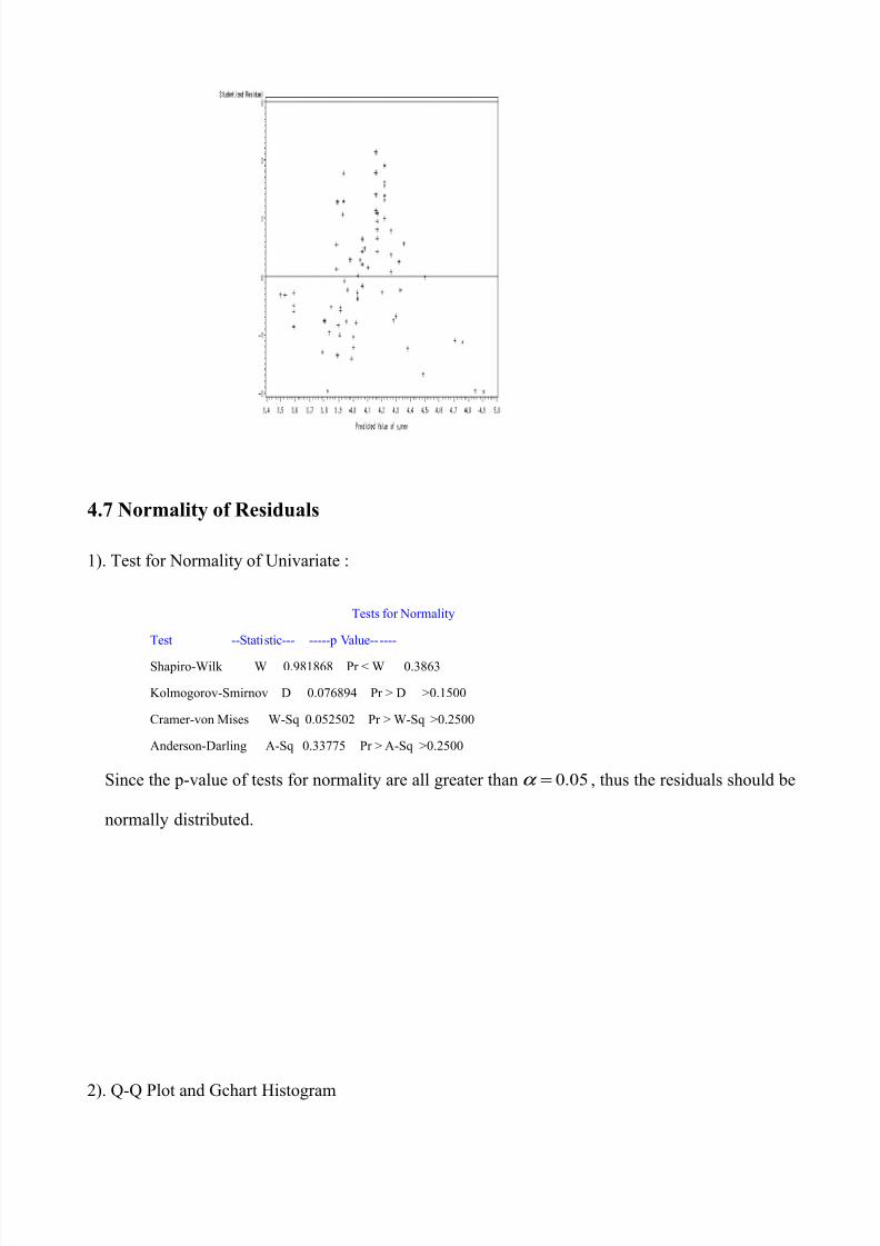
4.7 Outlier Checking
We can check the residuals by t-statistic. The residual would be an outlier if its t-statistic absolute
value is greater than 3. The following graph shows that there is no outlier in our residuals.
7/29/2019 proj Car Prices
http://slidepdf.com/reader/full/proj-car-prices 10/14
4.7 Normality of Residuals
1). Test for Normality of Univariate :
Tests for Normality
Test --Statistic--- -----p Value------
Shapiro-Wilk W 0.981868 Pr < W 0.3863
Kolmogorov-Smirnov D 0.076894 Pr > D >0.1500
Cramer-von Mises W-Sq 0.052502 Pr > W-Sq >0.2500
Anderson-Darling A-Sq 0.33775 Pr > A-Sq >0.2500
Since the p-value of tests for normality are all greater than 05.0=α , thus the residuals should be
normally distributed.
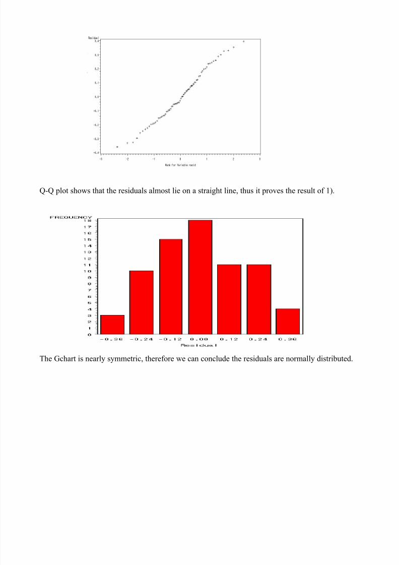
2). Q-Q Plot and Gchart Histogram
7/29/2019 proj Car Prices
http://slidepdf.com/reader/full/proj-car-prices 11/14
Q-Q plot shows that the residuals almost lie on a straight line, thus it proves the result of 1).
The Gchart is nearly symmetric, therefore we can conclude the residuals are normally distributed.
7/29/2019 proj Car Prices
http://slidepdf.com/reader/full/proj-car-prices 12/14
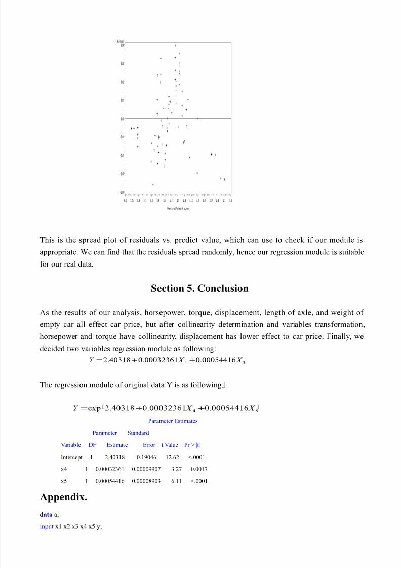
This is the spread plot of residuals vs. predict value, which can use to check if our module is
appropriate. We can find that the residuals spread randomly, hence our regression module is suitable
for our real data.
Section 5. Conclusion
As the results of our analysis, horsepower, torque, displacement, length of axle, and weight of
empty car all effect car price, but after collinearity determination and variables transformation,
horsepower and torque have collinearity, displacement has lower effect to car price. Finally, we
decided two variables regression module as following:
54 00054416.000032361.040318.2 X X Y ++=
The regression module of original data Y is as following:
5400054416.000032361.040318.2exp X X Y ++=
Parameter Estimates
Parameter Standard
Variable DF Estimate Error t Value Pr > |t|
Intercept 1 2.40318 0.19046 12.62 <.0001
x4 1 0.00032361 0.00009907 3.27 0.0017
x5 1 0.00054416 0.00008903 6.11 <.0001
Appendix.data a;
input x1 x2 x3 x4 x5 y;
7/29/2019 proj Car Prices
http://slidepdf.com/reader/full/proj-car-prices 13/14
cards;
0.01273 0.00309 1200 2000 990 31
0.01273 0.00309 1200 2000 820 31.2
0.02073 0.0048 1200 2470 1140 31.9
0.01273 0.00309 1200 2000 880 32.2
0.01273 0.00309 1200 2000 990 32.5
0.01273 0.00309 1200 2000 990 33.1
0.01273 0.00309 1200 2000 990 34.4
0.01217 0.0027 1200 2610 1000 35.1
0.01217 0.0027 1200 2610 1185 38.3
0.01217 0.0027 1200 2610 1080 38.9
0.01217 0.0027 1200 2610 1020 39.1
0.04724 0.02188 4000 2750 2220 90
0.024 0.0064 2000 2780 1690 90.9
0.04724 0.02188 4000 3350 2240 91
0.024 0.0064 2000 2780 1690 91.9
0.04724 0.02188 4000 3760 2260 92
0.02945 0.00558 2400 2750 1590 94.9
0.04724 0.02188 4000 3350 2345 96
0.024 0.0064 2000 2780 1690 96.9
0.04724 0.02188 4000 3760 2365 97
;
proc reg;
model y=x1-x5 /selection=stepwise slentry=0.1 slstay=0.2 details;
model y=x1 x2 x4 x5/vif ;
model y=x2 x4 x5/vif ;
model y=x4 x5/vif ;
model y=x4;
model y=x4 x5;
test x5;
model y=x4 x5 / covb;
output out=summary p=pred r =resid student=resid_sd;
proc gplot;
plot resid_sd*pred/ vref =(-3,0,3);
proc rank normal=blom;
var resid ;
ranks nscore;
proc univariate normal;
var resid;
proc gplot;

7/29/2019 proj Car Prices
http://slidepdf.com/reader/full/proj-car-prices 14/14
plot resid*nscore;
proc gchart;
vbar resid;
proc corr;
var resid nscore;
proc gplot;
plot resid*pred/vref =0 ;
run;