project management: a simulation-based optimization method
TRANSCRIPT

Rochester Institute of TechnologyRIT Scholar Works
Theses Thesis/Dissertation Collections
2009
Project management: a simulation-basedoptimization method for dynamic time-costtradeoff decisionsRadhamés A. Tolentino Pena
Follow this and additional works at: http://scholarworks.rit.edu/theses
This Thesis is brought to you for free and open access by the Thesis/Dissertation Collections at RIT Scholar Works. It has been accepted for inclusionin Theses by an authorized administrator of RIT Scholar Works. For more information, please contact [email protected].
Recommended CitationTolentino Pena, Radhamés A., "Project management: a simulation-based optimization method for dynamic time-cost tradeoffdecisions" (2009). Thesis. Rochester Institute of Technology. Accessed from
Rochester Institute of Technology
PROJECT MANAGEMENT: A SIMULATION-BASED OPTIMIZATION METHOD
FOR DYNAMIC TIME-COST TRADEOFF DECISIONS
A Thesis
Submitted in partial fulfillment of the
requirements for the degree of
Master of Science in Industrial Engineering
in the
Department of Industrial & Systems Engineering
Kate Gleason College of Engineering
by
Radhamés A. Tolentino Peña
January, 2009

i
DEPARTMENT OF INDUSTRIAL AND SYSTEMS ENGINEERING
KATE GLEASON COLLEGE OF ENGINEERING
ROCHESTER INSTITUTE OF TECHNOLOGY
ROCHESTER, NEW YORK
CERTIFICATE OF APPROVAL
M.S. DEGREE THESIS
The M.S. Degree Thesis of Radhamés A. Tolentino Peña
has been examined and approved by the
thesis committee as satisfactory for the
thesis requirement for the
Master of Science degree
Approved by:
____________________________________ Dr. Michael E. Kuhl, Thesis Advisor
____________________________________ Dr. Marcos Esterman

ii
ABSTRACT
Project managers face difficult decisions with regard to completing projects on time and
within the project budget. A successful project manager not only needs to assure that the project
is completed, but also desires to make optimal use of resources and maximize the profitability of
the project. The goal of this research is to address the time-cost tradeoff problem associated with
selecting from among project activity alternatives under uncertainty. Specifically, activities that
make up a project may have several alternatives each with an associated cost and stochastic
duration. The final project cost is a result of the time and cost required to complete each activity
and lateness penalties that may be assessed if the project is not completed by the specified
completion time. In an effort to optimize the project time-cost tradeoff, a dynamic, simulation-
based optimization method is presented. In particular, the method minimizes the expected project
cost due to lateness penalties and the activity alternatives selected. The method is designed to be
implemented in two phases. The first phase, referred to as the static phase, is implemented prior
to the start of the project. The static phase results in the expected cost for the recommended
project configuration including the alternative selected for each activity and the distributions of
the project completion and total project cost. The second phase, referred to as the dynamic phase,
is implemented as the project progresses. The dynamic phase allows the project manager to
reevaluate the remaining project and activity alternatives to dynamically minimize the expected
total project cost. The method provides an optimal solution under the assumptions of traditional
crashing implementations and a heuristic solution for the generalized problem. An experimental
performance evaluation shows the effectiveness of the method for making project management
decisions. Finally, the method is fully implemented in computer software and integrated into a
commercially available project management tool.
iii
TABLE OF CONTENTS
1. INTRODUCTION......................................................................................................................1
2. PROBLEM STATEMENT .......................................................................................................4
3. LITERATURE REVIEW .........................................................................................................7 3.1 Project Management: Project Scheduling ............................................................................ 7 3.2 Project Management: Time-Cost Tradeoffs ....................................................................... 12 3.3 Discrete Optimization via Simulation ................................................................................ 17 3.4 Discussion .......................................................................................................................... 18
4. OPTIMAL CRASHING METHODS FOR TRADITIONALLY DEFINED PROJECT MANAGEMENT PROBLEMS ..................................................................................................21
4.1 Assumptions Considered in the OTCM Method ................................................................ 24 4.2 OTCM Phase I: Optimal Crashing Method Applied Prior to the Start of the Project ....... 24 4.3 OTCM Phase I Example .................................................................................................... 27 4.4 OTCM Phase II: Dynamic Crashing .................................................................................. 32 4.5 OTCM Phase II Example ................................................................................................... 34 4.6 OTCM Optimization Program and OTCM Project Simulator ........................................... 43
4.6.1 OTCM - Input Files .................................................................................................... 46 4.6.2 OTCM - Simulation Model ........................................................................................ 47 4.6.3 OTCM - Optimization Engine .................................................................................... 50 4.6.4 OTCM - Project Simulator ......................................................................................... 51 4.6.5 OTCM - Integration of OTCM Program Components and the Project Simulator ..... 52
4.7 OTCM Experiments ........................................................................................................... 53 4.7.1 OTCM Experimental Case 1 ...................................................................................... 56 4.7.2 OTCM Experimental Case 2 ...................................................................................... 66 4.7.3 OTCM Experimental Case 3 ...................................................................................... 75 4.7.4 Summary of Experimental Performance Evaluation .................................................. 83
4.8 Summary of OTCM ........................................................................................................... 83
5. DYNAMIC SELECTION OF ACTIVITY ALTERNATIVES ...........................................84 5.1 Assumptions Considered in the DSA Method ................................................................... 87 5.2 DSA Phase I: Selection of Alternatives Prior to the Start of the Project ........................... 88 5.3 DSA Phase I Example ........................................................................................................ 91 5.4 DSA Phase II: Dynamic Selection of Alternatives during the Project Execution ............. 95 5.5 DSA Phase II Example....................................................................................................... 98 5.6 DSA Optimization Program and DSA Project Simulator ................................................ 102
5.6.1 DSA - Input Files ..................................................................................................... 105 5.6.2 DSA - Simulation Model .......................................................................................... 106 5.6.3 DSA - Optimization Engine ..................................................................................... 109 5.6.4 DSA - Project Simulator .......................................................................................... 110 5.6.5 DSA - Integration of DSA Program Components and the DSA Project Simulator . 111

iv
5.7 DSA Experiments ............................................................................................................ 112 5.7.1 DSA Experimental Case 1 ........................................................................................ 115 5.7.2 DSA Experimental Case 2 ........................................................................................ 123 5.7.3 Summary of Experimental Performance Evaluation ................................................ 131
5.8 Summary of DSA ............................................................................................................. 131
6. MS PROJECT INTERFACE ...............................................................................................133 6.1 OTCM Interface ............................................................................................................... 135 6.2 DSA Interface................................................................................................................... 142 6.3 Summary of OTCM and DSA MS Project Templates ..................................................... 148
7. CONCLUSIONS & RECOMMENDATIONS FOR FUTURE RESEARCH ..................149 7.1 Conclusions ...................................................................................................................... 149 7.2 Recommendations for Future Research ........................................................................... 151
REFERENCES ...........................................................................................................................152
APPENDICES ............................................................................................................................155 Appendix A. Industrial Strength COMPASS Input Parameters ............................................ 155 Appendix B. Input Files for OTCM Experimental Performance Evaluation......................... 157 Appendix C. Input Files for DSA Experimental Performance Evaluation ............................ 164 Appendix D. OTCM/DSA MS Project Template – User Manual ......................................... 169 Appendix E. CD Contents ...................................................................................................... 183

1
1. INTRODUCTION
Project management is a methodology used by many companies to help maximize
performance and competitiveness. Projects and their execution require resources which may
include people, equipments, materials, and energy. Project management, which is characterized
by techniques intended to provide a better use of project resources (Kerzner, 2003), can
positively impact the profitability of a company.
An important aspect of project management is risk management. Different types of risk
are present in any given project. This research focuses on the schedule/time risk and associated
costs. The schedule/time risk is a result of the uncertainty associated with completing project
activities on time and the potential late completion of the project. In general, late project
completion can have negative effects for the company such as penalty costs, budget overruns,
compromised project performance, customer dissatisfaction, lost market share, or lost revenue. If
a project is running late project managers might be able to bring the project back on track by
reducing the duration of the project’s activities through “the deployment of additional resources
or other means” (Eisner, 2002). For the purpose of this research, projects having activities with
multiple completion alternatives (activity alternatives) of varying completion times and costs are
considered. These activity alternatives could include outsourcing certain tasks, working
overtime, bringing in additional resources, and others. Although the activity alternatives may
reduce the project completion time, thus avoiding or reducing penalty costs, the incorporation of
these alternatives into the project may have additional cost. Furthermore, the duration of each
activity alternative may be uncertain. Provided that an estimate of the activity alternative
duration and the associated uncertainty can be obtained, the duration uncertainty can be taken
into consideration when selecting from among the various alternatives. The uncertainty of the

2
activity’s duration is commonly represented by a stochastic probability distribution. Given these
conditions, the objective of a project manager is to address the time-cost tradeoff associated with
selecting from among the activity alternatives, in order to choose the set of activity alternatives
that minimize the cost or maximize the profitability of the project. Without loss of generality,
this thesis frames this problem with the objective of minimizing total cost.
A conceptual representation of the time-cost tradeoff for a typical scenario involving a
planned project with a set of preferred (base) activity alternatives that has potential for being
completed late (resulting in a penalty), and may benefit from considering other activity
alternatives is illustrated in Figure 1.1. As various combinations of activity alternatives are
considered, the duration of the project may be reduced as well as the total cost of the alternatives
chosen plus the lateness penalty cost. For some combinations of activity alternatives, diminishing
returns may be realized until a point where the total cost may begin to increase. That is, some
combination of activity alternatives, although the combination would further reduce the
completion time of the project, the cost of using these sets of alternatives would cost more than
the penalty cost that would result from the project being late. Thus, the objective is to determine
the optimal set of activity alternatives associated with the point (indicated by the arrow) where
the total cost will be minimized. Determining the optimal time-cost tradeoff is the focus of this
research.
The rest of this thesis is organized as follows. Chapter 2 presents the problem statement
and states the goals of this research. Chapter 3 presents a review of the literature relevant to the
research which includes project scheduling, approaches to solving variations of the time-cost
tradeoff problem, and simulation-based optimization. Chapter 4 presents a dynamic simulation-
based crashing method capable of providing an optimal solution for the traditionally defined

3
stochastic time-cost tradeoff problem. Chapter 5 introduces a simulation-based optimization
method for the generalized dynamic time-cost tradeoff decision for project management. Chapter
6 illustrates the integration of the methods into Microsoft Project. Finally, Chapter 7 presents the
conclusions drawn from this research, as well as recommendations for future work.
Reduction in Project Duration
Alte
rnat
ives
+ P
enal
ty C
ost
Figure 1.1: Relationship between Reduction in Project Duration and the
Total Cost (Alternatives + Penalty).

4
2. PROBLEM STATEMENT
The goal of this research is to address the time-cost tradeoff problem associated with
selecting from among project activity alternatives under uncertainty. Specifically, activities that
make up a project may have several alternatives each with an associated cost and stochastic time
duration. The final project cost is a result of the time and cost required to complete each activity
and lateness penalties that may be assessed if the project is not completed by the specified
completion time. Therefore, a method is needed to evaluate the combination of activity
alternatives and their associated cost and to compare the resulting project completion times and
associated penalty costs to select the configuration that will minimize the total cost.
In an effort to optimize the project time-cost tradeoff, dynamic, simulation-based
optimization methods are investigated. The following are key objectives for this research:
• Develop a dynamic simulation-based optimization method for the traditionally defined
stochastic time-cost tradeoff problem: The traditionally defined stochastic time-cost
tradeoff problem focuses on projects in which the duration of the activities can be
reduced by integer time units having a constant cost per unit, and a penalty cost is
assessed if the project is completed late. Solving the traditionally defined time-cost
tradeoff problem involves identifying the activities whose duration is to be reduced and
the amount of the reduction (referred to as the crashing configuration) in order to
minimize the expected project cost due to lateness penalties and the cost of reducing the
activities duration. The method to be developed for solving this problem should be
capable of evaluating projects in the (static) planning phase (before the start of the
project) to determine the optimal crashing configuration that minimizes the average
project cost. The method should also be capable of dynamically reevaluating the project

5
as the project progresses. The information provided by the method to the project
managers should include the optimal crashing configuration and statistics associated with
the optimal solution (estimated average project cost, estimated project cost variance, and
a confidence interval on the average project cost), as well as an empirical distribution of
the project completion time and project cost for any potential crashing configuration.
• Develop a dynamic simulation-based optimization method for the generalized stochastic
time-cost tradeoff decision problem: The generalized stochastic time-cost tradeoff
problem focuses on projects in which the activities may have several alternatives each
with an associated cost and stochastic duration with the objective of determining the
configuration of alternatives that minimizes the expected project cost due to lateness
penalties and the cost of the alternatives selected. The method designed to solve this
problem should be capable of providing an optimal configuration of alternatives before
the start of the project and dynamically reevaluating the project throughout its execution.
The output of the method should include the optimal configuration of alternatives and
statistics associated with the optimal solution (estimated average project cost, estimated
project cost variance, and a confidence interval on the average project cost), as well as an
empirical distribution of the project completion time and project cost for any potential
configuration of alternatives.
• Implement the simulation-based optimization methods in a project management software
tool: The methods that are designed to solve the traditional and the general stochastic
time-cost tradeoff problems should be easy to apply to real projects in order to facilitate
their use. Consequently, the methods should be integrated into a commercially available
project management tool (such as Microsoft Project 2007) to create an interface through

6
which the methods can be applied. This implementation can allow the users to manage
their projects and utilize the simulation-based optimization tools for addressing the time-
cost tradeoff problem in a single application. Furthermore, the software tool should allow
for both the static (before the start of the project) and dynamic (during project execution)
use of the optimization methods. Finally, the software tool should provide the project
manager with the recommended activity alternative configuration, as well as the
supporting statistics and data to aid in their time-cost tradeoff decisions.
With the development of these robust, dynamic, and user-friendly simulation-based
optimization methods, project managers may be able to improve the use of their resources and
reduce the risk of late completion, thus contributing to a high level of customer satisfaction, and
profitability of their projects.

7
3. LITERATURE REVIEW
This chapter summarizes the current body of knowledge that is relevant to the research
conducted for this thesis, including project scheduling techniques, deterministic and stochastic
approaches to the time-cost tradeoff problem, and discrete optimization via simulation. The
potential contribution that this research can provide to the current literature is discussed at the
end of the chapter.
3.1 Project Management: Project Scheduling
The Critical Path Method (CPM) and the Project Evaluation and Review Technique
(PERT) methods have been used since the 1950s to assist in scheduling project activities. CPM is
a deterministic approach to calculate the completion time of a project, and PERT is a
probabilistic approach that considers uncertainty in activity durations to determine the
completion time of the project, and that can be used to estimate the probability to complete the
project by a given time (Wiest and Levy, 1969). CPM was originally developed for the type of
projects for which the information from previous similar projects could be used to estimate the
duration of the activities of the new project (such as construction projects), whereas PERT was
originally developed mainly for research and development projects, for which it is difficult to get
an estimate of the duration of each stage of the project (Wiest and Levy, 1969). In addition, CPM
is interested in the tradeoff between project cost and project completion time, and PERT is
interested in dealing with the uncertainty in activity durations (Wiest and Levy, 1969). Although
the original versions of CPM and PERT have some differences, they also have significant
similarities, and with time they have been commonly considered as one technique called
PERT/CPM (Hillier and Lieberman, 2001).

8
One of the common features between CPM and PERT is the way in which the completion
time of the project is estimated, which is using a project network to find the critical path of the
project. The project network is a graphical representation of the project, which shows the
dependence relationships between the activities of the project. From the project network one can
determine all of the network paths (set of project activities that connects the start and the end of
the project). CPM and PERT considers the length (time required to complete the activities on a
path) of the critical path as the estimated project duration. The critical path is the path with the
largest length; note that a project might have multiple critical paths. Hillier and Lieberman
(2001) show the procedure used by PERT/CPM to identify the critical path. The steps of the
procedure are:
• Determine the earliest start time (ES) and the earliest finish time (EF) of each activity.
This process starts at the beginning of the network and goes through all of the activities
until the end of the project network. This process is known as a forward pass. For each
activity EF is equal to ES plus the activity duration, and ES is equal to the largest EF
among the activity predecessors.
• Determine the latest start time (LS) and the latest finish time (LF) of each activity, by
making a backward pass through the network (opposite of making a forward pass). For
each activity LS is equal to LF minus the activity duration, and LF is equal to the smallest
LS among the activity successors.
• Determine the slack of each activity. The slack indicates the amount of time by which an
activity might be delayed without delaying the project completion time. For each activity
the slack is equal to LF minus EF. The activities with no slack belong to a critical path.

9
In calculating the critical path of the project, CPM considers that the duration of each
activity is known, whereas PERT (which considers uncertainty in activity duration) uses an
estimate of the expected duration of each activity. PERT deals with uncertainty by considering
three estimates of the activity duration [most likely (m), optimistic (o), pessimistic (p)], and
assuming that the distribution of the activity duration follows a beta distribution (Hillier and
Lieberman, 2001). Under that assumption the mean (µ) and the variance (σ2) of the beta
distribution that represent the activity duration can be approximated, respectively, by:
64 pmo ++
=µ and 2
2
6⎟⎠⎞
⎜⎝⎛ −
=opσ
.
Although PERT considers the mean and variance of each activity to describe its duration and
uncertainty, only estimates of the expected duration are considered to calculate the critical path,
ignoring the variances, thus making a deterministic analysis (Ahuja et al., 1994).
When there is uncertainty associated with the activity durations, it is important to know
the probability of completing the project by a certain time. PERT/CPM makes the following
assumptions to calculate this probability (Hillier and Lieberman, 2001):
• The mean critical path will be the path with the largest length. The mean critical path “is
the path through the project network that would be the critical path if the duration of each
activity equals its mean”.
• The durations for the activities in the mean critical path are statistically independent.
• The project duration follows a normal distribution.
From these assumptions it is possible to determine the mean project duration (µp), and the
variance of the project duration ( 2pσ ), which are needed to compute the probability of
completing the project by certain time. The mean project duration is equal to the length of the

10
mean critical path, and the variance of the project duration is equal to the sum of the variances of
the activities that form the mean critical path. Since the project duration is assumed to be a
normally distributed variable (X), the standard normal variable (Z) can be obtained using the
expression:
σµ−
=XZ .
The probability of completing the project by time x is then P(X ≤ x) = P(Z ≤ z), where σµ−
=xz .
A drawback of PERT stated by MacCrimmon and Ryavec (1964) is that when multiple
paths can be followed to complete a project, the calculated project duration “is always less than,
and never greater than, the true project mean.” This bias is identified as the “merge event bias”
and is most evident when the path durations are similar to each other. Conducting a stochastic
simulation study where the true properties of the distributions of activity duration are considered
can provide a better estimate of the expected completion time of the project (Ahuja et al., 1994).
Simulation of project networks has been used to improve the effectiveness of the
traditional PERT analysis. Williams (2004) indicates that Monte Carlo simulation of project
networks is now a common tool used by project managers. Simulating a project network
involves sampling an activity time from the probability distribution representing the duration of
each activity, and using the sampled activity duration to determine the critical path. Several
simulation-based project scheduling approaches are summarized in the next paragraphs.
The research of Lu and AbouRizk (2000) presents a CPM/PERT simulation model that
incorporates the discrete event modeling approach and a simplified critical activity identification
method. Lu and AbouRizk (2000) stated that “in the classic CPM analysis, earliest start time
(ES), latest start time (LS), earliest finish time (EF), latest finish time (LF), and total float (TF)

11
must be documented for every activity”. The ES and EF are calculated in a forward pass through
the project network and the LS, LF, and TF are calculated through a backward pass. TF is used to
determine the criticality of an activity. The simulation model that Lu and AbouRisk (2000)
presents only performs a forward analysis of the network; with this forward pass an entity arrival
time (AT), a batched entity departing time (DT) and a waiting time (WT) are calculated, instead
of ES and EF. The critical activity identification method presented by Lu and AbouRizk (2000)
uses the WT to calculate the criticality of each activity, which is represented by the criticality
index (CI); thus, all the information required to calculate the CI is collected during the forward
pass. The criticality index of an activity obtained through a simulation model “is defined as the
number of simulation runs in which the activity is critical, divided by the total number of
simulation runs” (Lu and AbouRisk, 2000).
Dong-Eun Lee (2005) presents a software tool, called Stochastic Project Scheduling
Simulation (SPSS), which can be used to determine the probability associated with the
completion of the project by a target date specified by the user of the software. The software has
the capability to simulate activity durations with several probability distribution functions, such
as normal, uniform, exponential and triangular distributions. SPSS also calculates activity
criticality indexes.
Lee and Arditi (2006) describe a new simulation system, called Stochastic Simulation-
based Scheduling (S3), which is an improvement over SPSS. The drawbacks of PERT are also
referenced in that publication, and it is stated that “compared with the simulation method, PERT
leads to and optimistically biased project duration, since PERT inherently ignores all subcritical
paths”. An advantage of S3 over SPSS is that S3 calculates a confidence interval for the project

12
mean duration and also determine the minimum number of simulation runs necessary to achieve
reliable results.
Pritsker (1986) and Simmons (2002) also describe simulation models that evaluate
project networks. These simulation models provide a histogram of the project completion time
distribution, which can be used to perform risk analysis.
3.2 Project Management: Time-Cost Tradeoffs
When scheduling a project there are certain key dates that the project manager must
consider, such as the target completion time desired by the customer, and the deadline for the
project to be considered as completed early. Usually, if the project is completed after the target
completion time, a penalty due to lateness is assessed, and if the project is completed before the
deadline for early completion, a bonus is realized. In some cases the project manager may realize
that with the current resources it is not possible to complete the project by the early completion
deadline, or by the target completion time. However, there are cases were the duration of certain
project activities can be reduced (using measures that have an additional cost) in order to avoid
penalties due to lateness or to receive bonuses for early completion. Since business decision are
generally made based on cost, in cases like the one previously described the project manager has
to evaluate the tradeoff between the reduction in project duration and the additional cost
associated with that reduction, to determine if it make economic sense to expedite the completion
of the project.
A method for addressing the time-cost tradeoffs present in a project is the CPM method
of time-cost tradeoffs (Hillier and Lieberman, 2001); from this point forward this method will be
referred to as the CPM crashing method. This method is focused on finding the crashing

13
configuration with the lowest cost that reduces the project estimated duration to a preferred
value. The crashing configuration indicates which activities should be crashed and by how much
should they be crashed. Hillier and Lieberman (2001) indicate that crashing an activity is to take
measures (involving an additional cost) to reduce the duration of an activity, such as working
overtime, bringing in additional temporary help, or using special equipment. Rosenau and
Githens (2005) state crashing is “spend[ing] more money on the project in order to speed up
accomplishment of scheduled activities”. To apply the CPM crashing method it is required to
have the crashing potential of each activity, which represents the maximum reduction of time
allowed by the activity (note that the crashing potential cannot be greater than the estimated
duration of the activity in order to avoid negative activity time), as well as the crashing cost per
time unit. The method assumes that reducing the duration of an activity that belongs to the
critical path by 1 unit reduces the duration of the project by 1 unit. The CPM crashing method
generally assumes that the crashing cost increases linearly as the crashed amount increases. The
CPM crashing method is generally implemented using linear programming (Hillier and
Lieberman, 2001).
The CPM crashing method has one major limitation which is the fact that it only
considers the estimated average duration of the activities, ignoring the uncertainty related with
the duration of the activities. Considering uncertainty is important because it allows having a
better understanding of the real impact that a crashing configuration will have on the project
duration. Since only the estimated average activity durations are considered, when a project is
crashed the expected completion time of the project (which is the mean of the distribution that
represents the completion time) is approximated to the desired target. Therefore, the probability
to complete the project by the target is 50% (see Figure 3.1); in cases where there are multiple

14
critical paths the probability may be smaller (Haga and Marold, 2004). If the probability
distributions that represent the activity durations are considered in the crashing process, it is
possible to shift the distribution of completion time to a point where the probability for late
completion is relatively low.
Original Completion Time
TargetTime
Original Completion Time
TargetTime
Traditional Crashing
Stochastic Crashing
Figure 3.1: Traditional Crashing vs. Stochastic Crashing.
As a way to overcome the limitations of the CPM crashing method, several simulation-
based crashing methods that address the time-cost tradeoff problem have been developed (Bissiri
and Dunbar, 1999; Gutjahr et al., 2000; Haga, 1998; Haga and Marold, 2004; Haga and Marold,
2005), but in general the literature about this topic is limited (Herroelen and Leus, 2005). The
objective of these methods is to obtain the optimal crashing configuration that minimizes the

15
project cost (lateness penalty plus crashing cost). The next paragraphs summarize some of these
methods.
Bissiri and Dunbar (1999) present a method to crash a project network, which suggest the
use of simulation to obtain the average time of each activity, the critical path, and the near
critical paths. A near critical path in this model is a path which length is smaller than the original
completion date but it is larger than the target completion date after crashing. After the path
information is collected a linear program is applied to determine the optimum crashing strategy.
This method works in a very similar way to the traditional CPM crashing method because it
considers average activity times and looks for a solution in a deterministic manner.
Gutjahr et al. (2000) introduces a stochastic branch-and-bound crashing method, which
objective is to select the set of measures that will reduce the duration of the project, avoiding or
reducing penalty costs, in the most cost-efficient way. Specifically, it is assumed that there is a
group of measures that can be implemented, and each measure may reduce the duration of one or
more activities in the project by a given amount. Each measure is associated with a binary
variable which indicates if the measure is chosen or not.
Haga (1998) along with Haga and Marold (2004), and Haga and Marold (2005) present a
series of papers involving heuristic crashing methods for project management utilizing
simulation.
Haga and Marold (2004), proposed a simulation-based method that deals with the time-
cost trade-off involved with crashing a project. The authors state that “the complete distribution
of project completion time needs to be considered when crashing”. The method that they
proposed is a two steps approach. The first step is to apply the traditional PERT method to crash
the project, and the second step consists of testing each activity that had not been crashed up to

16
its limit to determine if crashing that activity further reduces the average total cost of the project.
In this research, the authors considered two sources that can increase the cost of the project,
which are crashing costs and overrun costs. The approach that Haga and Marold (2004) followed
tries to optimize the cost of the project, thus if the penalty for late completion is smaller than the
crashing cost of the activities this method may suggest to allow the project to be completed late.
One improvement opportunity identified in this research is that the method presented does not
provide a way to monitor the crashing recommendations that it proposes, which can result in
unnecessary crashing of activities. The approach presented in Haga and Marold (2004) is a
heuristic that doesn’t consider interactions between different activities; essentially it conducts a
one-at-a-time evaluation of the crashing potential of the activities to determine which activities
should be crashed.
As a continuation of the Haga and Marold (2004) research, Haga and Marold (2005)
developed a simulation-based method to monitor and control a project. The output of this method
is a list of dates at which the project manager “should review the project to decide if activities
need to be crashed”. These dates are called crashing points, and they are determined by a
backward run through the project network. Although the concept explained in this research is
very useful, the proposed method requires a large amount of simulation time to evaluate a large
project network and “if the network does not have a single dominant critical path, the algorithm
will likely tend to overly crash the project” (Haga and Marold, 2005). In addition, before the
project starts, this method determines which activities might be crashed.
The methods discussed in this section provide a foundation for solving the time-cost
tradeoff problem in project management.

17
3.3 Discrete Optimization via Simulation
When dealing with the stochastic time-cost tradeoff problem, the project managers are
interested in identifying the optimal crashing configuration that minimizes the project cost. Since
the simulation-based crashing methods currently described in the literature are heuristic, there is
an opportunity to develop a method capable of providing an optimal solution to the stochastic
time-cost tradeoff problem.
In the context of simulation, discrete optimization is designed to “maximize or minimize
the expected value of a simulation output random variable whose distribution depends on a finite
vector of controllable decision variables” (Xu et al., 2007). In the case of the stochastic time-cost
tradeoff problem the objective is to minimize the expected value of the project cost which
depends on a vector of integer variables that represent the crashing amount of each activity
Various solution methods for discrete optimization via simulation are presented in the
literature, “including globally convergent random search (GCRS) algorithms, locally convergent
random search (LCRS) algorithms, ranking and selection (R&S), and ordinal optimization (OO)”
(Xu et al., 2007). For additional details please refer to Xu et al. (2007).
One of the most recent algorithms for discrete optimization via simulation is Industrial
Strength COMPASS (ISC). ISC is “a particular implementation of a general framework for
optimizing the expected value of a performance measure of a stochastic simulation with respect
to integer-ordered decision variables” (Xu et al., 2007). ISC is derived from the Convergent
Optimization via Most Promising Area Stochastic Search (COMPASS) framework developed by
Hong and Nelson (2006) for locally convergent, discrete optimization-via-simulation (DOvS).
As indicated by Xu et al. (2007), ISC provides convergence guarantees and statistical inference.
Commercial software for optimization via simulation (OvS) are able to provide results to

18
realistic problems in a reasonable amount of time; however, they lack the convergence
guarantees and statistical inference that ISC provides.
ISC is an initial effort to close the gap that commercial OvS software have in terms of
convergence guarantees, thus it has limitations (Xu et al., 2007):
• Problems with multiple objectives are not supported;
• Only integer-ordered decision variables are considered;
• Only linear-integer inequality constraints are considered; and
• Recommended for problems with up to 10 decision variables.
Although these limitations exist, ISC can be applied to a large segment of discrete simulation
optimization problems.
The optimization procedure implemented by ISC is divided in three phases:
• Global Phase: explores the entire solution space, and identifies sub-regions with potential
good solutions;
• Local Phase: evaluates each sub-region and converges to local optimal solutions; and
• Clean Up Phase: selects the best solution among the local optima identified in the Local
Phase, and estimates its value with the precision specified by the user.
Since the stochastic time-cost tradeoff problem is a problem suitable for DOvS, ISC is a
good candidate for an optimization engine.
3.4 Discussion
While reviewing literature relevant to the time-cost trade-off problem in project
management, certain opportunities for improvement have been identified. One opportunity is
found in the fact that the crashing methods in the current literature are primarily heuristic in

19
nature and provide a solution to the problem, but do not guarantee optimality. To address this
opportunity a simulation-based crashing method (presented in Chapter 4) is developed in which a
simulation model interacts with an optimization engine to obtain an optimal solution. Another
opportunity is that the simulation-based methods that are presented in Section 3.2 are designed to
solve only a portion of the problems that project managers may face. To expand the current
literature a method is developed (and presented in Chapter 5) to solve a generalized version of
the stochastic time-cost tradeoff problem, which relaxes the assumptions considered by the
traditionally defined time-cost tradeoff problem.
From the methods presented in Section 3.2, the methods that are more closely related (in
terms of the solution the method provides) to the methods presented in this thesis are Haga and
Marold (2004, 2005). Table 3.1 summarizes these methods and the ones presented in this thesis.
Regarding the traditionally defined time-cost tradeoff problem, in the case of a single
critical path the method of Haga and Marold (2004) provides an optimal solution in the static
phase, which is prior to the start of the project. For the dynamic phase (throughout the project
execution) Haga and Marold (2005) provides a heuristic solution; essentially the method
provides, prior to the start of the project, a set of completion times (crashing points) for the
activities by which the activities should be completed, and then, during the project, the project
manager needs to decide if the activities will be completed by those points; if the project
manager decides that the activities won’t be completed by the crashing points, the activities
should be crashed. For the case of multiple potential critical paths Haga and Marold (2004)
provide a heuristic solution for the static phase. The dynamic solution (Haga and Marold 2005) is
heuristic as well and can over-crash the project.

20
The first method developed and presented in this thesis (OTCM), which is focused on the
traditionally defined time-cost tradeoff problem, provides (for the static evaluation) an optimal
solution for the cases of single or multiple critical paths. For the dynamic phase OTCM is a
heuristic solution because the user specifies the times for the dynamic reevaluations. If the
project is continuously reevaluated the solution would be optimal.
Table 3.1. Summary of Different Approaches to the Time-Cost Tradeoff Problem (CP ≡ Critical Path).
Static Method (Haga & Marold,
2004)
Dynamic Method (Haga & Marold,
2005)
Static Method Dynamic Method
Single CP; Integer Crashing; Linear Costs Optimal Heuristic Optimal
(OTCM) Heuristic (OTCM)
Multiple CP; Integer Crashing; Linear Costs Heuristic Heuristic Optimal
(OTCM) Heuristic (OTCM)
Single/Multiple CP; Varying Mean of Base Alternative; Non-linear, ordered Costs
- - Heuristic (DSA)
Heuristic (DSA)
Single/Multiple CP; Varying Distribution of Base Alternative; Non-linear, not ordered Costs
- - Heuristic (DSA)
Heuristic (DSA)
In addition, a method that more accurately represent the situations that the project
manager might encounter has been developed. The method (DSA) relaxes the assumptions
traditionally associated with the alternatives associated to each activity. DSA is a heuristic
because the optimization engine used is not designed to guarantee optimality for these cases. If
an optimization engine can be developed for these cases the solutions provided can be optimal.

21
4. OPTIMAL CRASHING METHODS FOR TRADITIONALLY DEFINED
PROJECT MANAGEMENT PROBLEMS
Although the intention of this research is to solve the generalized time-cost tradeoff
problem, the initial methods that are developed and presented are for the traditionally defined
application of crashing methods to project management. Given that much of the current literature
(e.g. Bissiri and Dunbar, 1999; Gutjahr et al., 2000; Haga and Marold, 2004) focuses on the
traditional definition of crashing and assuming that this definition adequately describes a portion
of the projects to which project management techniques are applied, optimal crashing methods
for this traditionally defined scenario are presented in this chapter. The methods developed for
the generalized time-cost tradeoff problem are presented in Chapter 5.
Project management problems involving crashing are traditionally defined as follows.
Given a project defined by individual activities, their precedence relationships, and stochastic
activity durations, a project network can be developed. An example of such a project (Sample
Project) having 11 activities is described in Table 4.1; Figure 4.1 illustrates the project network
where the nodes represent the activities and the arcs (edges) represent the precedence
relationships. In this type of project, crashing is defined as “spend[ing] more money on the
project in order to speed up accomplishment of scheduled activities” (Rosenau and Githens,
2005). The crashing potential of an activity is the maximum number of time units by which an
activity’s time can be reduced. In this traditional definition, activities are typically crashed in
integer time units up to the crashing potential, and the associated crashing cost is assumed to be
linear (that is, each time unit by which the activity is crashed has the same cost). For each
activity in the example, the maximum crashing potential is specified in Table 4.1 along with the
associated linear crashing cost per time unit. If the project is late, a lateness penalty is assessed as

22
a linear function of the quantity of time by which the project is late. For example, a project that is
due at time 70 with a lateness penalty of 40 per time unit would have the following penalty
function,
⎩⎨⎧
>−≤
=70τif),70τ(4070τif,0
)τ,(TPF.
The objective of the traditionally defined problem is to determine the activities to crash
in order to minimize the average project total cost, where the total cost is defined as crashing cost
plus any penalty due to lateness.
Table 4.1: Sample Project Specifications. Activity Duration Crashing Unit Crashing
Activity Predecessors Minimum Mode Maximum Potential Cost 1 - 8 10 12 3 6 2 1 6 10 14 3 3 3 1 6 8 10 3 5 4 3 10 15 20 3 4 5 2 12 17 22 3 5 6 2,4 3 5 7 3 8 7 5 6 9 12 3 5 8 6 4 6 8 3 5 9 4 11 13 15 3 2 10 7,8,9 13 15 17 3 8 11 10 5 7 9 3 7
1
2
3
4
7
6
5
8
9
10 11
Figure 4.1: Sample Project Network.

23
The purpose of this first stage of the research is to develop static and dynamic simulation-
based analysis methods for the traditionally defined time-cost tradeoff problem that are capable
of evaluating project networks to answer the following questions:
• Which activities should be crashed in order to minimize the average project cost?
• To what extent should the activities be crashed?
• Should the crashing configuration be changed throughout the project?
The method presented in this section is named the Optimal Traditional Crashing Method
(OTCM). The overall OTCM procedure is presented in two phases. Phase I considers the
evaluation of the project prior to the start of the project. This phase will produce an optimal
crashing strategy with respect to information available prior to the start of the project. During
Phase II, which is applied as the project progresses, dynamic reevaluations of the project are
performed in order to consider the known durations (and sunk costs) of completed activities and
the effect of the uncertainty of the durations of the remaining activities, and to determine the
optimal crashing strategy from that point forward.
In the next sections, Phase I and Phase II of the OTCM procedure are presented.
Although the two phases are designed to be used together to maximize the benefit of the method,
Phase I can be applied independently from Phase II at the start of the project with Phase II being
optional.

24
4.1 Assumptions Considered in the OTCM Method
The OTCM method is designed taking the following assumptions into account:
1) Crashing an activity is defined as reducing the activity time by an integer number of time
units, thereby shifting the location of the distribution and maintaining the shape
(variance, skewness, etc.) of the activity time distribution;
2) Activity times are independent;
3) Activity time distributions can be estimated, using a probability distribution that will not
result in negative activity times when crashing is applied. Using the beta distribution or
the triangular distribution to represent activity times is common in the field of project
management (Lee and Arditi, 2006; Lu and AbouRizk, 2000; Haga and Marold, 2004)
and this convention is kept for the OTCM examples and experiments. The probability
distribution of each activity, in this case, is defined by three estimates consisting of the
optimistic (minimum), most likely, and pessimistic (maximum) duration times;
4) Crashing costs are known or can be estimated very accurately;
5) Penalty costs for late completion, represented by a linear function, are defined before the
start the project; and
6) Precedence constraints are assumed to be strictly defined (a successor activity cannot
begin until all the predecessors have been completed).
4.2 OTCM Phase I: Optimal Crashing Method Applied Prior to the Start of the Project
The objective of Phase I of the method is to obtain the optimal crashing configuration
prior to the start of the project that will minimize the expected total project cost with respect to
crashing costs and penalty costs. Since this phase is implemented before the start of the project
25
the uncertainty associated with the duration of each activity is considered, which is represented
by probability distributions.
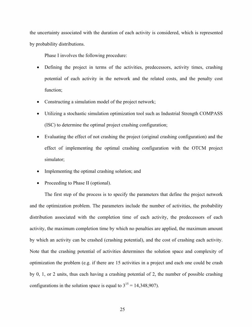
Phase I involves the following procedure:
• Defining the project in terms of the activities, predecessors, activity times, crashing
potential of each activity in the network and the related costs, and the penalty cost
function;
• Constructing a simulation model of the project network;
• Utilizing a stochastic simulation optimization tool such as Industrial Strength COMPASS
(ISC) to determine the optimal project crashing configuration;
• Evaluating the effect of not crashing the project (original crashing configuration) and the
effect of implementing the optimal crashing configuration with the OTCM project
simulator;
• Implementing the optimal crashing solution; and
• Proceeding to Phase II (optional).
The first step of the process is to specify the parameters that define the project network
and the optimization problem. The parameters include the number of activities, the probability
distribution associated with the completion time of each activity, the predecessors of each
activity, the maximum completion time by which no penalties are applied, the maximum amount
by which an activity can be crashed (crashing potential), and the cost of crashing each activity.
Note that the crashing potential of activities determines the solution space and complexity of
optimization the problem (e.g. if there are 15 activities in a project and each one could be crash
by 0, 1, or 2 units, thus each having a crashing potential of 2, the number of possible crashing
configurations in the solution space is equal to 315 = 14,348,907).

26
A simulation model of the project network is constructed after the input parameters are
provided. The simulation model represents all the activities in the project and the precedence
relationships that exist among them. The model is used to evaluate the various crashing
configurations that could be implemented in the project. Evaluating a crashing configuration
involves running a specified number of replications (instances) of the project network, under the
crashing configuration that is being considered, in order to estimate the average project cost
resulting from that configuration. Running a replication of the simulation model representing the
project network involves sampling an activity time from the probability distribution representing
the duration of each activity, reducing the sampled duration according to the crashing
configuration that is being considered, calculating the start time and completion time of each
activity taking into account that precedence relationships must be enforced, calculating the
completion time of the project, calculating the penalty for late completion (if any), and finally
computing the project cost, which consists of the lateness penalty and the crashing cost.
Once the simulation model has been designed, and the crashing potential for each activity
on the network has been identified, it is possible to run the optimization (OTCM program). The
simulation-based optimization engine for the OTCM method is designed to optimize the
performance measure generated by the simulation model, given that the performance measure
depends on integer decision variables. The optimization engine also provides convergence
guarantees within a precision level specified by the user. The stochastic optimization is
responsible for minimizing the average cost subject to constraints that indicate that the crashing
amount of each activity cannot be greater than its crashing potential. The engine searches the
solution space for potential optimal solutions. Once a potential solution (crashing configuration)
is found it is sent to the simulation model for evaluation. The simulation model then runs a

27
specified number of instances of the project for the crashing configuration sent by the
optimization engine and calculates the cost of the project in each instance; the number of
instances to be evaluated is determined by the optimization engine. The cost of each evaluated
instance of the project is sent to the stochastic optimization engine which tests the configuration
for optimality. The optimization engine continues the evaluation of potential solutions until the
optimal solution has been identified. At that point, the optimal solution is reported, which
includes the crashing configuration that minimizes the average project cost and statistics
associated with the optimal solution (sample mean of project cost, sample variance of project
cost, and a 95% confidence interval on project cost).
After obtaining the optimal solution, the OTCM project simulator is used to evaluate the
impact that implementing the original or the optimal crashing configuration has on the project
cost. The output of the project simulator includes statistics about the project completion time and
project cost (sample mean, sample variance, and a 95% confidence interval), and provides the
data required to plot the distributions of project completion time and project cost under both
crashing configurations (original vs. optimal). Using these pieces of information, the project
manager can decide if the optimal crashing configuration will be implemented. The project
manager also decides if Phase II will be applied.
4.3 OTCM Phase I Example
To illustrate Phase I of the OTCM method, the Sample Project discussed in Section 4 is
used. The details are shown again here for convenience in Table 4.2 and Figure 4.2. In this
example, the project network consisting of 11 activities has multiple potential critical paths and
the penalty cost is considerably bigger than the crashing cost of any activity in the network. Each

28
activity in this project has a crashing potential of up to 3 time units. The respective estimates of
the minimum, most likely, and maximum activity times used to fit a beta distribution to the
activity durations, and the crashing costs per unit are shown in Table 4.2. The target completion
time of the project is time 70, and the equation defining the penalty cost for late completion is
⎩⎨⎧
>−≤
=70τif),70τ(4070τif,0
)τ,(TPF
where τ is the resulting completion time of the project. Figure 4.3 depicts the input file used in
this example (see Section 4.6.1 for a detailed discussion of input file parameters).
Table 4.2: OTCM Phase I Example - Project Specifications. Activity Duration Crashing Unit Crashing
Activity Predecessors Minimum Mode Maximum Potential Cost 1 - 8 10 12 3 6 2 1 6 10 14 3 3 3 1 6 8 10 3 5 4 3 10 15 20 3 4 5 2 12 17 22 3 5 6 2,4 3 5 7 3 8 7 5 6 9 12 3 5 8 6 4 6 8 3 5 9 4 11 13 15 3 2 10 7,8,9 13 15 17 3 8 11 10 5 7 9 3 7
1
2
3
4
7
6
5
8
9
10 11
Figure 4.2: OTCM Phase I Example - Project Network.

29
n 11 T 70 P 40 SC 0 NPi 0 1 1 1 1 2 1 1 1 3 1
0 1
1 3
2 2 4
5 6 4 7 8 9 10
CPi 3 3 3 3 3 3 3 3 3 3 3 B8 10 12 B6 10 14 B6 8 10 B10 15 20
Activity B12 17 22 Duration B3 5 7 Distribution B6 9 12 (Ai) B4 6 8
B11 13 15 B13 15 17 B5 7 9 6 3 5 4 5
Crash Costs 8 (CCi) 5
5 2 8 7
ISC output Parameters 999999 1 0 -1 -1 0 -1 1 -1 -1 -1 0.01 1 0.01 0.5 50 10 0 50
Figure 4.3: OTCM Phase I Example - Input File.
Predecessors (PMij = 1 for each j in row i, i = 1,…,n)

30
The OTCM program was used to obtain the optimal crashing configuration which is to
crash activity 2 two time units, and activity 9 one time unit, with an estimated average project
cost of 14.55 and an associated project cost variance of 435.56 (the OTCM program ran 22,686
replications to compute these estimates). The 95% confidence interval on the average project
cost when the solution provided by Phase I is implemented is:
[14.28 ≤ 0µ ≤ 14.82].
The original project without crashing and the project with the optimal crashing configuration are
each simulated 50,000 times with the OTCM project simulator to produce the distribution of
completion time (Figure 4.4) and the cumulative distribution of the total project cost (Figure
4.5). In addition, Table 4.3 provides the average and standard deviation of the project duration
and project cost.
0%2%4%6%8%
10%12%14%16%18%20%
58 60 62 64 66 68 70 72 74 76 78
Prob
abili
ty
Duration original
optimal Figure 4.4: OTCM Phase I Example - Original versus Optimal Project Completion Time.

31
0%10%20%30%40%50%60%70%80%90%
100%
0 50 100 150 200 250 300 350
Cum
mul
ativ
e %
Cost original
optimal Figure 4.5: OTCM Phase I Example - Original versus Optimal Project Cost.
Table 4.3: OTCM Phase I Example - Summarized Comparison between No Crashing and
Optimal Crashing. Duration Cost Average Std. Dev. Average Std. Dev. Original 69.22 2.11 20.41 38.73 Optimal 67.85 2.06 14.35 20.43
To provide statistical evidence about the cost reduction produced by the Phase I method
over no crashing, using paired data a 95% confidence interval is built on the difference between
the average cost of the project when no crashing is applied and the project when the solution
provided by Phase I is implemented:
[5.85 ≤ 50000,01µ ≤ 6.28].
These results indicates that there is a significant difference between the average cost of no
crashing versus the average cost of implementing the Phase I solution, and indicates that when
the optimal crashing configuration is implemented the average cost of the project is reduced.

32
4.4 OTCM Phase II: Dynamic Crashing
In Phase I, prior to the start of the project, an initial optimal crashing configuration is
obtained by analyzing the entire project network. This initial optimal crashing configuration
considers the uncertainty associated with the duration of all the activities of the project. As
activities are completed, the uncertainty associated with their duration is eliminated. Thus the
overall uncertainty about the project completion time is reduced; as a result the initial optimal
solution might change. The purpose of the Phase II (dynamic) method is to determine the optimal
crashing configuration for the remaining activities.
In addition to the general assumptions of the OTCM method, the following assumptions
are applied to Phase II:
• The reevaluations points occur just prior to starting an activity that has been
recommended for crashing previously. The initial reevaluation points are assumed as the
crashing points identified in Phase I;
• The resources required to crash an activity are available at the moment of making a
crashing decision, i.e. the lead time to acquire or change the resources is 0; and
• The remaining time for activities in progress is known or can be estimated very
accurately.
Due to the first assumption, Phase II is a heuristic. In order for Phase II to be optimal
throughout the project, the project network should be constantly evaluated. Constantly evaluating
the project is not practical and cost prohibitive, thus, in this research it has been assumed that the
project is reevaluated when the start time of an activity identified to be crashed is encountered
(the intention of the reevaluations in this case is to verify if the activity still needs to be crashed
or not; if the predecessors activities are completed in a time shorter than expected it is likely that

33
the activity doesn’t need to be crashed or needs to be crashed by a smaller amount). In addition,
the first assumption indicates that if no activities should be crashed, according to the solution
provided by Phase I, there is no need to implement Phase II. However, although not tested here
the project manager could decide implementing Phase II at any time after the start of the project,
in order to determine if crashing would make economic sense due to the duration of activities
previously completed, or as changes are made to the project plan.
The OTCM Phase II procedure involves:
1. Updating the project information to reflect the current status of the project;
2. Updating the simulation model of the project network;
3. Reevaluating the remaining project network using the OTCM program (as described in
Phase I) when an activity that requires crashing is encountered;
4. Evaluating the effects of implementing the previous crashing configuration and the new
optimal crashing configuration with the OTCM project simulator;
5. Implementing the project network under the new crashing configuration and continuing
until either:
a) the next activity that requires crashing is encountered and go to step 1; or
b) the project is complete.
Note that for each iteration of steps 1-4 of the dynamic crashing procedure, a new
crashing configuration for the remainder of the project will be identified that takes into account
the sunk activity times and costs associated with the activities in progress and the activities that
have been completed.
The first step in the procedure that Phase II follows is to update the information that
defines the current status of the project. For the activities completed or in progress, their crashing

34
potential is set to 0 and their duration is represented by their actual (in the case of completed
activities) or estimated (in the case of activities in process) duration (instead of by a probability
distribution). For the activities that haven’t started the crashing potential, the crashing cost, and
the probability distribution of completion time are considered to be equal to the values used in
Phase I. Also, Phase II considers the same target completion time and the same penalty function
used in Phase I (note that since the project information is updated before each reevaluation it is
possible to include information different than the one provided in Phase I or in previous Phase II
reevaluations). The updated information is input into the simulation model to guarantee that the
simulation model is an accurate representation of the project network.
After the simulation model is updated the optimization process, as described in Phase I, is
applied. Then, the optimal crashing configuration provided by the OTCM program and the
previous crashing configuration are evaluated with the OTCM project simulator. As in Phase I,
the project manager uses the output of the OTCM project simulator to decide whether or not to
implement the solution provided by the Phase II reevaluation. This process continues until
another reevaluation point is encountered or until the project is complete.
4.5 OTCM Phase II Example
The Sample Project used to illustrate Phase I is now used to demonstrate Phase II of the
OTCM method. Recall, that the Sample Project consisted of 11 activities with the project details
outlined in Table 4.2 and the corresponding project network shown in Figure 4.2. The optimal
crashing configuration obtained when Phase I of the OTCM was applied to the Sample Project
specified that activity 2 should be crashed two time units and activity 9 should be crashed one
time unit. Given this information, the project can begin. (Although not occurring in this example,

35
if any of the activities that start at the project starting time are recommended by Phase I to be
crashed, the crashing should be applied.) To facilitate a direct comparison among project
implementations with no crashing applied, using the result of OTCM Phase I only, and the full
implementation of the OTCM method (Phases I and II), one instance of the Sample Project is
simulated. The resulting activity times without any crashing applied are shown in Table 4.4.
After the project begins, the OTCM Phase II procedure specifies that the project
reevaluation points (the points at which the crashing configuration is reevaluated) will occur just
prior to starting activities that have previously been identified by the OTCM method to be
crashed. In the Sample Project, at time 10.88 which corresponds to the completion time of
activity 1, the first activity that Phase I specified to crash is encountered. Consequently, the time
just prior to the start of activity 2 will serve as the reevaluation point. Figure 4.6 depicts the
status of the project up to the first reevaluation point.
Table 4.4: OTCM Phase II Example - Sample Project Instance. Activity Duration
1 10.88 2 7.32 3 8.15 4 17.91 5 15.75 6 4.87 7 7.95 8 4.86 9 13.35 10 15.82 11 6.54
To implement the reevaluation, the OCTM program is invoked with an input file that
reflects the current project status. This input file is shown in Figure 4.7. The bold entries indicate
the updates required from the initial OTCM Phase I implementation. (Note that in this Sample

36
Project, the crashing potential for each of the remaining activities remains the same throughout
the project. However, any changes to the project parameters including the activity durations and
crashing potential can be updated at any time and included in the reevaluation.) Thus, the
updates to the input file needed for this reevaluation include changing the crashing potential of
activity 1 to 0 and entering the actual duration of activity 1 as a constant time of 10.88 (indicated
as C10.88 in the input file, where C denotes a constant).
Legend:Completed & Not Crashed
In process & Not Crashed
Completed & Crashed
In process & Crashed
Not Started
Evaluation Point
2
3
4
7
6
5
8
9
10 111
Figure 4.6: OTCM Phase II Example - Network Status by First Reevaluation Point.
Upon running the OTCM program, a new crashing configuration is obtained for the
remaining activities. Table 4.5 shows the resulting crashing configuration which specifies that
activity 2 is to be crashed two time units (this in consistent with the result of Phase I), and since
the project is lagging due to a longer than expected duration of activity 1, the crashing
configuration also specifies crashing activity 9 by two time units (rather than 1 time unit as
specified by Phase 1). Table 4.6 indicates the new estimate of the average project cost (Sample
Mean of Cost) and the associated estimate of the project cost variance (Sample Variance of Cost)

37
which are 19.06 and 601.48, respectively. In addition, the number of simulated instances of the
project used to obtain the estimates, 30,856 replications, is also listed.
n 11 T 70 P 40 SC 0 NPi 0 1 1 1 1 2 1 1 1 3 1
0 1
1 3
2 2 4
5 6 4 7 8 9 10
CPi 0 3 3 3 3 3 3 3 3 3 3 C10.88 B6 10 14 B6 8 10 B10 15 20
Activity B12 17 22 Duration B3 5 7 Distribution B6 9 12 (Ai) B4 6 8
B11 13 15 B13 15 17 B5 7 9 6 3 5 4 5
Crash Costs 8 (CCi) 5
5 2 8 7
ISC output Parameters 999999 1 0 -1 -1 0 -1 1 -1 -1 -1 0.01 1 0.01 0.5 50 10 0 50
Figure 4.7: OTCM Phase II Example - Input File First Reevaluation.
Predecessors (PMij = 1 for each j in row i, i = 1,…,n)

38
Table 4.5: OTCM Phase II Example - Crashing Configuration Provided by First Reevaluation. Activity 1 2 3 4 5 6 7 8 9 10 11 Crash
Amount 0 2 0 0 0 0 0 0 2 0 0
Table 4.6: OTCM Phase II Example - Summary of Solution Provided by First Reevaluation. Replications 30,856
Sample Mean of Cost 19.06 Sample Variance of Cost 601.48
Upon implementing the specified crashing amount of 2 time units for activity 2, the
project proceeds until the next reevaluation point in encountered. This occurs just prior to the
start of activity 9 which is realized at time 36.94. By that time activities 1 through 5 have been
completed, activity 7 is in progress, and the remaining activities haven’t started. Figure 4.8
shows the status of the project up to the second reevaluation point. The input file of the OTCM
program is updated once again to reflect the current project status. The update includes setting
the crashing potential of activities 1 through 5 to 0 and replacing the probability distribution that
previously represented their duration by their actual duration; since activity 7 is in progress its
crashing potential is also set to 0 and its duration (assumed to be accurately estimated) is
considered to be a constant time of 7.95. In addition, the input file is updated to include the sunk
cost of crashing activity 2; since activity 2 was crashed twice and the crashing cost per time unit
of activity 2 is equal to 3, the sunk cost is equal to 6. After updating the input file the OTCM
program is executed, and a new crashing configuration is obtained. Table 4.7 shows the new
crashing configuration which indicates that activity 9 is to be crashed three time units (even more
than previously indicated by the first reevaluation), and since the project continues to run behind
schedule, the crashing configuration indicates crashing activities 8 and 11 by one time unit each.

39
Table 4.8 shows the new estimates for the average project cost and the project cost variance
which are 24.84 and 23.19, respectively (545 instances of the project were simulated to obtain
these estimates).
Legend:Completed & Not Crashed
In process & Not Crashed
Completed & Crashed
In process & Crashed
Not Started
Evaluation Point
6 8
9
10 111
5
3
4
72
Figure 4.8: OTCM Phase II Example - Network Status by Second Reevaluation Point.
Table 4.7: OTCM Phase II Example - Crashing Configuration Provided by Second Reevaluation.
Activity 1 2 3 4 5 6 7 8 9 10 11 Crash
Amount 0 2 0 0 0 0 0 1 3 0 1
Table 4.8: OTCM Phase II Example - Summary of Solution Provided by Second Reevaluation. Replications 545
Sample Mean of Cost 24.84 Sample Variance of Cost 23.19
Activity 9 is crashed three time units as indicated by the crashing configuration, and the
project continues. The new reevaluation point is encountered at time 41.81, which corresponds to
the start time of activity 8. By that time activities 6 and 7 have also been completed, and activity
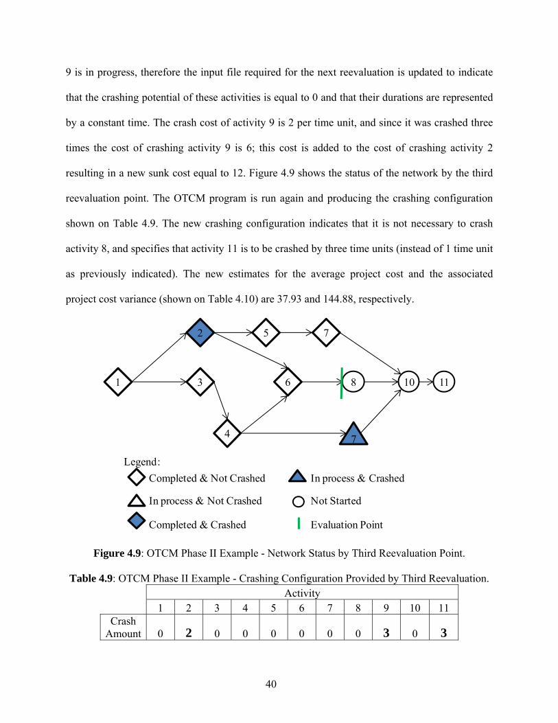
40
9 is in progress, therefore the input file required for the next reevaluation is updated to indicate
that the crashing potential of these activities is equal to 0 and that their durations are represented
by a constant time. The crash cost of activity 9 is 2 per time unit, and since it was crashed three
times the cost of crashing activity 9 is 6; this cost is added to the cost of crashing activity 2
resulting in a new sunk cost equal to 12. Figure 4.9 shows the status of the network by the third
reevaluation point. The OTCM program is run again and producing the crashing configuration
shown on Table 4.9. The new crashing configuration indicates that it is not necessary to crash
activity 8, and specifies that activity 11 is to be crashed by three time units (instead of 1 time unit
as previously indicated). The new estimates for the average project cost and the associated
project cost variance (shown on Table 4.10) are 37.93 and 144.88, respectively.
Legend:Completed & Not Crashed
In process & Not Crashed
Completed & Crashed
In process & Crashed
Not Started
Evaluation Point
8 10 111
5
3
4
2
6
7
7
Figure 4.9: OTCM Phase II Example - Network Status by Third Reevaluation Point.
Table 4.9: OTCM Phase II Example - Crashing Configuration Provided by Third Reevaluation. Activity 1 2 3 4 5 6 7 8 9 10 11 Crash
Amount 0 2 0 0 0 0 0 0 3 0 3

41
Table 4.10: OTCM Phase II Example - Summary of Solution Provided by Third Reevaluation. Replications 9,653
Sample Mean of Cost 37.93 Sample Variance of Cost 144.88
The project proceeds and the next reevaluation point is encountered at time 63.11, which
corresponds to the completion time of activity 10 and start time of activity 11. Figure 4.10
depicts the status of the project network up to the fourth reevaluation. By that time, activities 1
through 10 are completed and the sunk cost remains 12. The input file of the OTCM program is
updated accordingly, and the OTCM program is run. The new crashing configuration, presented
in Table 4.11, specifies that activity 11 is to be crashed by three time units. The new estimates
for the average project cost and the project cost variance are 46.21 and 283.18, respectively (see
Table 4.12). In order to obtain these estimates 15,290 instances of the project were simulated.
Legend:Completed & Not Crashed
In process & Not Crashed
Completed & Crashed
In process & Crashed
Not Started
Evaluation Point
111
5
3
4
2
6
7
8
7
10
Figure 4.10: OTCM Phase II Example - Network Status by Fourth Reevaluation Point.

42
Table 4.11: OTCM Phase II Example - Crashing Configuration Provided by Fourth Reevaluation.
Activity 1 2 3 4 5 6 7 8 9 10 11 Crash
Amount 0 2 0 0 0 0 0 0 3 0 3
Table 4.12: OTCM Phase II Example - Summary of Solution Provided by Fourth Reevaluation. Replications 15,290
Sample Mean of Cost 46.21 Sample Variance of Cost 283.18
After implementing the crashing configuration the project reaches its completion. The
crash cost of activity 11 is 7 per time unit, resulting in a crashing cost of 21. Therefore, the
cumulative crashing cost for Phase II is equal to 33 (previous sunk cost plus crashing cost of
activity 11). The completion time of the project is 66.65; therefore, no penalty cost is assessed.
The total cost of this instance of the project is 33.
Table 4.13 indicates the final crashing configurations provided by Phase I and Phase II. If
only the solution provided by Phase I would have been implemented, the completion time of the
project would have been 71.65; therefore, a penalty of 66 would have been assessed. The total
crashing cost of the crashing configuration provided by Phase I is equal to 8, thus, the total cost
of the project would have been 74. On the other hand, if the original project would have been
implemented the completion time would have been 72.65, resulting in a total project cost of 106
(due to the lateness penalty). Table 4.14 summarizes the results of the three implementations.
Implementing only Phase I resulted in a 30% reduction in the total project cost, and
implementing the Phase II resulted in an impressive 69% reduction in the total project cost.

43
Table 4.13: OTCM Phase II Example - Crashing Configurations Provided by Phase I and Phase II.
Activity Phase 1 2 3 4 5 6 7 8 9 10 11
Phase I 0 2 0 0 0 0 0 0 1 0 0 Phase II 0 2 0 0 0 0 0 0 3 0 3
Table 4.14: OTCM Phase II Example - Original vs. Phase I vs. Phase II. Cost
Phase Completion Time Crashing Penalty Total Original 72.65 0 106 106 Phase I 71.65 8 66 74 Phase II 66.65 33 0 33
To provide statistical support about the benefit of implementing Phase II over just
implementing Phase I, 500 instances of the project are simulated and their results are used to
build a 95% confidence interval on the difference between (paired observations) the average
project cost of the project when Phase I is implemented and the project when the Phase II is
implemented:
[3.32 ≤ 500,12µ ≤ 5.63].
The results indicate that the project cost when only Phase I is implemented is significantly higher
than the project cost when the full OTCM is implemented.
4.6 OTCM Optimization Program and OTCM Project Simulator
The optimization program used in Phase I and Phase II of the OTCM method to obtain an
optimal crashing configuration has three main components: the input file, the OTCM program
containing the simulation model and the optimization engine, and the output files containing the
performance measures of the optimal solution identified. The interaction between the

44
components of the optimization program, which is the same for Phase I and Phase II, is shown in
Figure 4.11. The difference between Phase I and Phase II, with respect to the optimization
program, is in the input and the OTCM program which considers in Phase II the portion of the
project that has been completed and the associated sunk costs, and optimizes the crashing
configuration for the remainder of the project.
PROJECT PARAMETERS
(n, Ai, PM, T, P, CPi, CCi, SC)
OPTIMIZATION ENGINE
Minimizes.t.xi ≤ CPi ∀i = 1,…,n
SIMULATION MODEL
C = PF(T , τ) + + SC
x
C
OPTIMAL CRASHING CONFIGURATION
- Sample Mean of Project Cost- Sample Variance of Project Cost
- 95% CI on Project Cost
OTCM Program
Input File
Output Files
Figure 4.11: Components of the OTCM Optimization Program.
C∑=
n
iii xCC
1

45
As part of the OTCM procedure, once an optimal solution is identified the OTCM project
simulator is used to compare the impact that implementing the new optimal crashing
configuration or the previous crashing configuration has on the average project cost and the
average project completion time. The OTCM project simulator has the following components:
the input file, the simulation model, and the output file containing statistics about the project cost
and the project completion time for each one of the configurations evaluated. Figure 4.12 depicts
the interaction between the components of the OTCM project simulator.
PROJECT PARAMETERS
(n, Ai, PM, T, P, CCi, SC, x)
CURRENT & OPTIMAL CRASHING CONFIGURATIONS
- Sample Mean of Project Cost & Duration
- Sample Variance of Project Cost & Duration
- 95% CI on Project Cost & Duration- Distribution of Project Cost &
Duration
SIMULATON MODEL
Input File
Output Files
Figure 4.12: Components of the OTCM Project Simulator.

46
A detailed explanation about the components of the OTCM optimization program and the
OTCM project simulator is presented in the next sections.
4.6.1 OTCM - Input Files
The input file of the OTCM optimization program includes the following information:
• First line: number of activities in the project (n);
• Second line: target completion time (T);
• Third line: penalty cost per unit of lateness (P);
• Fourth line: sunk cost (SC);
• Fifth line: number of predecessors per activity (NPi ∀i = 1,…,n);
• Next n lines: predecessors of activity (PMij = 1 for each j in row i, i = 1,…,n);
• Next line: crashing potential for activity i (CPi ∀i = 1,…,n);
• Next n lines: distribution of duration of activity i = 1,…,n;
• Next n lines: crash cost of activity i = 1,…,n;
• Next line: name of the output file to be generated by the optimization engine (ISC); and
• Next line: parameters required by the optimization engine (ISC; see Appendix A).
The input file of the OTCM project simulator requires the following information:
• First line: number of activities in the project (n);
• Second line: target completion time (T);
• Third line: penalty cost per unit of lateness (P);
• Fourth line: sunk cost (SC);
• Fifth line: number of predecessors per activity (NPi ∀i = 1,…,n);

47
• Next n lines: predecessors of activity (PMij = 1 for each j in row i, i = 1,…,n);
• Next line: crashing configuration to be evaluated (x = <x1, x2,…, xn>);
• Next n lines: distribution of duration of activity i = 1,…,n; and
• Next n lines: crash cost of activity i = 1,…,n.
4.6.2 OTCM - Simulation Model
The simulation model used in the OTCM program and in the OTCM project simulator
was created in the C++ programming language. The simulation model was created in this
programming language to facilitate its interaction with Industrial Strength COMPASS (also
developed in C++), which is the optimization engine chosen for this research. The simulation
model is used to determine the expected project duration and the expected project cost (crashing
cost plus penalty cost); the latter represents the objective function of the optimization.
In order to define the project network to be represented by the simulation model it is
necessary to capture relevant information about the project. The following constants are created
for that purpose:
n ≡ number of activities in the project.
Ai ≡ distribution of the duration of activity i = 1,…,n.
S ≡ set of completed or in process activities (in Phase I, S = {∅}).
R ≡ set of remaining activities (in Phase I, R includes all project activities).
T ≡ target completion time.
P ≡ penalty cost per time unit of lateness.
NPi ≡ number of predecessors of activity i = 1,…,n.

48
PM ≡ predecessors matrix; PMij is equal to 1 if activity i is preceded by activity j, 0
otherwise, ∀i,j = 1,…,n,
PM =
⎥⎥⎥⎥⎥⎥
⎦
⎤
⎢⎢⎢⎢⎢⎢
⎣
⎡
nnn
n
PMPM
PMPMPMPM
...................................................
......
1
21
11211
.
CPi ≡ crashing potential (maximum number of units by which the activity can be crashed)
for activity i = 1,…,n, CPi = 0 ∀i ∈ S.
CCi ≡ unit crash cost of activity i = 1,…,n.
di ≡ actual or accurately estimated duration of activity i ∈ S.
y ≡ vector of crashed time units for activity i = 1,…,n, yi ≥ 0 for i ∈ S, yi = 0 for i ∈ R.
SC ≡ sunk cost; define as the cost of the activities previously crashed, ∑∈
=n
SiiiCCySC .
The following variables are used in the simulation model algorithm that simulates an instance of
the project to estimate the project completion (τ) time and the project cost (C):
x ≡ vector of n integer decision variables (x = <x1, x2,…, xn>), where each decision
variable (xi) represents the number of time units by which activity i is crashed,
∀i = 1,…,n, where xi = 0 for i ∈ S.
PCi ≡ number of predecessors of activity i already completed ∀i = 1,…,n.
ti ≡ duration for activity i = 1,…,n.
sti ≡ start time of activity i = 1,…,n.
cti ≡ completion time of activity i = 1,…,n.
ACi ≡ is set to 1 if activity i is completed, 0 otherwise, ∀i = 1,…,n.

49
PF(T,τ) ≡ linear function that represents the penalty for late completion.
For each replication of the simulation model (a simulated instance of the project) the
following algorithm is applied:
1) Set sti = cti = PCi = ACi = 0 ∀i = 1,…,n;
2) If activity i ∈ R, generate ti from Ai; otherwise ti = di ∀i = 1,…,n;
3) Set index i = 1;
4) If ACi = 0 and PCi = NPi go to step 5, otherwise go to step 9;
5) If PMij = 1, sti = max(sti,ctj) ∀j = 1,…,n;
6) Set cti = sti + ti – xi;
7) If PMji = 1, PCj = PCj + 1 ∀j = 1,…,n;
8) Set ACi = 1; if ∑=
=n
ii nAC
1 go to step 10;
9) If i = n, set i = 1; otherwise i = i + 1; go to step 4;
10) Set τ = max(cti ∀i = 1,…,n);
11) Set C = PF(T,τ) + ∑=
n
iii xCC
1
+ SC.
In the simulation model used by the OTCM project simulator the value of xi is assigned
by the user, and in the simulation model used by the OTCM program the value of xi is generated
by the optimization engine.
In order to verify the simulation model, multiple replications are run. For each
replication, the pieces of information generated by the simulation model are output and recorded.
Those pieces of information are: activity time sampled for each activity, total crashing cost, total
penalty cost, total cost, and project completion time. Please note that other pieces of information

50
used to verify the simulation model such as target completion time, crashing configuration
applied to a particular replication, crashing cost of each activity, and penalty cost per time unit of
lateness are provided as input, thus they are available before running each replication. All the
information recorded from the replications along with the information input into the simulation
model is used to verify the results by hand. When verifying each replication, the following
conditions are evaluated:
• Activity time sampled for each activity felt in the range of possible values corresponding
to the probability distribution function from which the activity time was sampled.
• Activities are crashed by the amounts specified in the crashing configuration that is input.
• The project completion is consistent with the sampled activity times, taking into
consideration that some of the sampled activity times were reduced due to crashing.
• The crashing cost of each replication is consistent with the crashing amount and the
crashing cost of each activity.
• Penalty cost is consistent with project completion time. If project completion time is less
or equal than the target completion time, no penalty cost is applied; if it is greater than the
target, the penalty cost increased according to the penalty cost per time unit of lateness
provided as input.
• The total project cost is the sum of the crashing cost and the penalty cost.
4.6.3 OTCM - Optimization Engine
The simulation model uses integer decision variables that represent the number of time
units by which an activity is crashed; a particular set of values for these integer decision
variables represents a crashing configuration. The simulation model interacts with an

51
optimization engine with the purpose of determining the crashing configuration that generates
the minimum average total cost (C ). The optimization engine is responsible for selecting the
crashing configuration to be evaluated; for each one of these crashing configurations the
expected total cost is computed. Finally the optimization engine determines the crashing
configuration that minimizesC .
The optimization engine used in this step of the methodology is Industrial Strength
COMPASS (ISC) (Xu et al., 2007). ISC is a tool which is derived from the COMPASS
framework developed by Hong and Nelson (2006) for locally convergent, discrete optimization-
via-simulation (DOvS). To utilize ISC the C++ simulation model is integrated into the ISC code.
ISC requires inputs such as an initial solution, the range of possible values for each decision
variable (CPi ∀i =1,…,n), the precision within which the optimal solution is to be found (δ), and
the confidence level associated to the solution (α); these inputs must be provided in a separate
text file from which ISC reads them. ISC provides a default value for most of the input
parameters. Appendix A includes the complete list of inputs required by ISC (for additional
information about the ISC input parameters please refer to Xu et al. 2007). ISC searches the
feasible region defined by the potential activities that can be crashed and returns an optimal
solution within the specified tolerance.
4.6.4 OTCM - Project Simulator
The OTCM project simulator is designed to evaluate the impact that a particular crashing
configuration has on the project in terms of project completion time and project cost. Although
the OTCM project simulator can be used to evaluate any crashing configuration, it is developed
with the intention of estimating time and cost statistics of the project network when the optimal

52
crashing configuration obtained in a particular evaluation of the project network and when the
previous optimal crashing configuration are applied. Note that the previous crashing
configuration considered for Phase I is usually not to crash any activity, and for Phase II the
previous crashing configuration is usually the optimal crashing configuration identified at the
previous reevaluation.
The complete list of inputs required by the project simulator is presented in section 4.6.1.
The outputs of the OTCM project simulator include an estimate of the average project cost and
the average project completion time, an estimate of the variance of the project cost and the
project completion time, and a 95% confidence interval on the average project cost and the
average project completion time. In addition, the output includes all the data points used to
calculate the estimates, which can also be used to plot the distributions of project cost and project
completion time.
4.6.5 OTCM - Integration of OTCM Program Components and the Project Simulator
The following algorithm summarizes the steps required by the Phase I or Phase II of the
OTCM method:
Step 1: Define the project network by setting the values of n, T, P, Ai, PMij, NPi, CCi
∀i,j = 1,…,n.
Step 2: Define the optimization problem by setting the values of CPi ∀i = 1,…,n, and setting
the values of the inputs required by the optimization engine such as δ and α.
Step 3: Input the simulation model into an optimization engine and solve the optimization
problem, which follows the following format:

53
Minimize C where C = PF(T , τ) + ∑=
n
iii xCC
1 + SC
s.t.
xi ≤ CPi ∀i = 1,…,n
Step 4: Run multiple replications (the number of replications is specified by the user) of the
project network using the OTCM Project Simulator, implementing both the original
crashing configuration and the optimal crashing configuration, to estimate the average
and the standard deviation of the project cost, to construct a confidence interval on the
average project cost, and to plot the distribution of project cost.
4.7 OTCM Experiments
To investigate the ability of the OTCM method to consistently provide optimal crashing
configurations in both Phase I and Phase II, an experimental performance evaluation is
conducted. In particular, the experiments are designed to test the robustness of the OTCM
method to determine the optimal crashing configuration in terms of minimizing the expected
total cost for traditionally defined project management crashing problems. The experimental
performance evaluation focuses on three main factors including a) the complexity of the project
network in terms of the number of potential critical paths; b) the size of project network in terms
of the number of activities; and c) the relative uncertainty (variability) in activity time durations.
Experimental test cases are constructed to evaluate each of the three main factors. Each
case consists of two networks that are used to evaluate the factors at two different levels. These
cases are as follows:

54
• Case 1: Complexity of the project network
A. A project network with a single critical path
B. A project network with multiple potential critical paths
• Case 2: Size of the project network
A. A project network having 13 activities
B. A project network having 24 activities
• Case 3: Uncertainty in activity time durations
A. A project with relatively low variability in activity time durations
B. A project with relatively high variability in activity time durations.
For each experiment, the Phase I (static) and Phase II (dynamic) OTCM methods are applied and
evaluated.
To evaluate Phase I and Phase II of the OTCM method, the following procedure is used.
For each factor level within each case, a project having the necessary characteristic is
selected. Several of the projects are taken directly from or slightly modified from projects in the
literature (e.g. Haga, 1998; Haga and Marold 2004; Haga and Marold, 2005). The remainder of
the projects has been arbitrarily selected to have the characteristic of interest.
The OTCM Phase I and Phase II are applied to each project. The project specifications
including the activity time distributions, activity predecessors, crashing cost, and penalty costs
are specified in the input file. The input files are displayed in Appendix B. For activities that can
be crashed in each project, the crashing potential is specified to be 3 time units, except for the
experimental Case 2B in which the crashing potential is 5 time units. For Phase I, the OTCM
program is run to obtain the optimal crashing configuration that minimizes the expected total
cost (crashing cost plus lateness penalty cost). Finally the OTCM project simulator is used to

55
simulate 50,000 instances of the original project and the project with the OTCM Phase I crashing
configuration implemented. The data from the 50,000 instances of each system is then used to
construct empirical graphs of the distribution of completion time and the cumulative distribution
of total cost. The estimated average and standard deviation of the project completion time and
project cost is also presented for both systems. In addition, a 95% confidence interval (using
paired data) is constructed on the difference between the mean total cost of the original project
and the project with the optimal crashing configuration, referred to as 50000,01µ .
For Phase II, the optimal crashing configuration obtained in Phase I is used as the starting
point for each project. Multiple instances of each project are generated. The number of instances
generated is dependent on the particular project (i.e., enough instances are generated to identify
if there is a significant difference between the average project cost when Phase I is implemented
and the average project cost when Phase II is implemented). For each project instance, the
OTCM Phase II is applied. Each instance of the project is simulated applying no crashing, the
optimal crashing configuration provided by Phase I, and the optimal crashing configuration
provided by Phase II. The resulting completion times and total costs under each case are
recorded for each instance, and the estimated average and standard deviation of the project cost
and project completion time are presented. Finally, two 95% confidence intervals are
constructed. The first confidence interval is constructed on the difference between the average
total cost of the original project and the project with the Phase I crashing configuration applied,
and the second confidence interval is constructed on the difference between the average total cost
of the project with the Phase I crashing configuration applied and the project after the OTCM
Phase II has been applied. The confidence intervals are referred to as N,01µ and N,12µ ,
respectively, where N represents the number of instances generated for each experimental case.

56
Since Phase I is evaluated before the project starts, it might be evaluated using the
standard version of the optimization tool (program that connects the simulation model and the
optimization engine), which is designed to conduct an evaluation of the network at a specified
point of time. In order to make the experimental process more efficient for Phase II an automated
version of the optimization tool was created. This version has the following features:
• Evaluate Phase I of the network and record the optimal crashing configuration;
• Sample random times from Ai ∀i = 1,…,n for each instance of the project to be used as
the real duration (without crashing) of each activity;
• Keep track of the most recent crashing configuration and its related sunk cost; and
• Determines the reevaluation points and reevaluates the network accordingly.
4.7.1 OTCM Experimental Case 1
Case 1 of the experimental performance evaluation demonstrates the ability of the OTCM
method to obtain an optimal solution for projects having one or multiple critical paths. Case 1A
considers a project with 1 dominant critical path, and Case 1B considers a project with multiple
potential critical paths.
4.7.1.1 Case 1A: A Project Having a Single Critical Path
Case 1A considers a project with a single critical path. The project network used in this
experiment is based on an experiment presented by Haga (1998) and Haga and Marold (2005).
The project network is depicted graphically in Figure 4.13. Table 4.15 shows the 36 activities in
the network along with the precedence relationships. This network contains only 1 critical path
which will be the focus of this experiment. This single dominant critical path is highlighted by
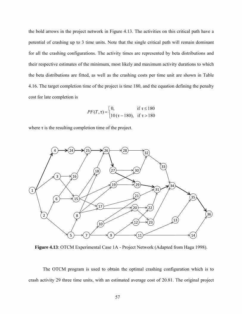
57
the bold arrows in the project network in Figure 4.13. The activities on this critical path have a
potential of crashing up to 3 time units. Note that the single critical path will remain dominant
for all the crashing configurations. The activity times are represented by beta distributions and
their respective estimates of the minimum, most likely and maximum activity durations to which
the beta distributions are fitted, as well as the crashing costs per time unit are shown in Table
4.16. The target completion time of the project is time 180, and the equation defining the penalty
cost for late completion is
⎩⎨⎧
>−≤
=180τif),180τ(10180τif,0
)τ,(TPF
where τ is the resulting completion time of the project.
1
2
3
4
7
6
5
8
9
12
14
1310
11
15
17
16
20
18
22
19
21
23
24 25 26
27
29
28
30
3431
32
33
35
36
Figure 4.13: OTCM Experimental Case 1A - Project Network (Adapted from Haga 1998).
The OTCM program is used to obtain the optimal crashing configuration which is to
crash activity 29 three time units, with an estimated average cost of 20.81. The original project

58
without crashing and the project with the optimal crashing configuration are each simulated
50,000 times to produce the distribution of completion time (Figure 4.14) and the cumulative
distribution of the total project cost (Figure 4.15). In addition, Table 4.17 provides the average
and standard deviation of the project duration and project cost.
Table 4.15: OTCM Experimental Case 1A - Dependency Relationships of Project Network.
Activity Predecessors Activity Predecessors1 - 19 8, 15 2 1 20 10, 17 3 1 21 10, 17 4 1 22 12, 20 5 2 23 12,20 6 2 24 4 7 5 25 16, 24 8 5 26 18, 25 9 7 27 26 10 7 28 26 11 9 29 19, 27 12 9 30 19, 27 13 11 31 21, 22, 29 14 11 32 28, 30 15 3, 6 33 32 16 3, 6 34 23, 31, 33 17 8, 15 35 13, 34 18 8, 15 36 14, 35
Table 4.16: OTCM Experimental Case 1A - Minimum (a), Most Likely (ml), and Maximum (b) Duration, and Crashing Cost for Each Activity.
Activity a ml b Crash Cost 1 10 20 30 9 4 12 14 16 8 24 14 18 22 4 25 12 18 30 6 26 10 20 30 9 27 8 12 16 9 29 18 25 32 1 31 10 20 30 8 34 15 20 25 9 35 6 12 18 4

59
0%
2%
4%
6%
8%
10%
12%
14%
16%
140 150 160 170 180 190 200 210 220
Prob
abili
ty
Duration original
optimal
Figure 4.14: OTCM Experimental Case 1A - Original vs. Optimal Project Completion Time.
0%10%20%30%40%50%60%70%80%90%
100%
0 50 100 150 200 250 300 350 400
Cum
mul
ativ
e %
Cost original
optimal
Figure 4.15: OTCM Experimental Case 1A - Original vs. Optimal Project Cost.
Table 4.17: OTCM Experimental Case 1A - Summarized Comparison between No Crashing and
Optimal Crashing. Duration Cost Average Std. Dev. Average Std. Dev. Original 179.99 7.66 30.60 44.76 Optimal 176.99 7.66 20.96 34.40

60
The 95% confidence interval on the difference of the means 50000,01µ between the average
cost of the project when no crashing is applied and the average cost of the project when the
solution provided by Phase I is implemented is:
[9.52 ≤ 50000,01µ ≤ 9.77].
In evaluating Phase II, 600 instances of the project are generated. Each instance of the
project is simulated implementing the original project, Phase I, and Phase II. Table 4.18
summarizes the results.
Table 4.18: OTCM Experimental Case 1A - Summarized Comparison between Original Project, Phase I, and Phase II.
Duration Cost Average Std. Dev. Average Std. Dev. Original 180.25 7.63 31.83 46.10 Phase I 177.25 7.63 21.98 35.67 Phase II 177.04 6.19 18.23 30.16
The 95% confidence interval on the difference of the means 600,01µ between the average
cost of the original project and the average cost of the project when Phase I is implemented is:
[8.71 ≤ 600,01µ ≤ 10.98].
The 95% confidence interval on the difference of the means 600,12µ between the average
cost of the project when Phase I is applied and the average cost of the project when Phase II is
implemented is:
[3.11 ≤ 600,12µ ≤ 4.40].

61
4.7.1.2 Case 1B: A Project Having Multiple Critical Paths
Case 1B considers a project with multiple potential critical paths. This experiment is
based on the project network previously shown in section 4.3. For completeness, the graphical
representation of the project network (Figure 4.16), and the table describing the precedence
relationships and the estimates of activity duration used to fit the probability distribution of each
activity (Table 4.19) are shown again. All the activities on this network have a crashing potential
of up to 3 time units. The activity times are represented by triangular distributions, and the target
completion time of the project is time 70. The equation defining the penalty cost for late
completion is
⎩⎨⎧
>−≤
=70τif),70τ(4070τif,0
)τ,(TPF
where τ is the resulting completion time of the project.
Table 4.20 shows the criticality indexes of the activities in the project network, which
indicates the probability that each activity has to be in the critical path when no crashing is
applied.
1
2
3
4
7
6
5
8
9
10 11
Figure 4.16: OTCM Experimental Case 1B - Project Network.

62
Table 4.19: OTCM Experimental Case 1B - Activity Duration Information, Crashing Cost, and Predecessors for Each Activity.
Activity a m b Crash cost Predecessors 1 8 10 12 6 - 2 6 10 14 3 1 3 6 8 10 5 1 4 10 15 20 4 3 5 12 17 22 5 2 6 3 5 7 8 2,4 7 6 9 12 5 5 8 4 6 8 5 6 9 11 13 15 2 4 10 13 15 17 8 7,8,9 11 5 7 9 7 10
Table 4.20: OTCM Experimental Case 1B - Criticality indexes. Activity Criticality index
1 1 2 0.512 3 0.488 4 0.488 5 0.512 6 0.017 7 0.512 8 0.017 9 0.471 10 1 11 1
The optimal solution encountered by the OTCM program is to crash activity 2 twice and
activity 9 once, resulting in an estimated average project cost of 14.55. In order to build the
distributions of completion time and cost, 50,000 replications of both the original and optimal
configurations are run. Figure 4.17 shows both the distribution of project completion time when
no crashing is applied and when the optimal crashing configuration obtained from Phase I is
applied. Figure 4.18 shows the cumulative cost distributions corresponding to the each case.

63
0%2%4%6%8%
10%12%14%16%18%20%
58 60 62 64 66 68 70 72 74 76 78
Prob
abili
ty
Duration original
optimal
Figure 4.17: OTCM Experimental Case 1B - Original vs. Optimal Project Completion Time.
0%10%20%30%40%50%60%70%80%90%
100%
0 50 100 150 200 250 300 350
Cum
mul
ativ
e %
Cost original
optimal
Figure 4.18: OTCM Experimental Case 1B - Original versus Optimal Project Cost.
The results from the 50,000 simulated instances of the project are summarized in Table
4.21. The 95% confidence interval on the difference of the means 50000,01µ between the average
cost of the project when no crashing is applied and the average cost of the project when the
solution provided by Phase I is implemented is:

64
[5.85 ≤ 50000,01µ ≤ 6.28].
Table 4.21: OTCM Experimental Case 1B - Summarized Comparison between no Crashing and Optimal Crashing.
Duration Cost Average Std. Dev. Average Std. Dev. Original 69.22 2.11 20.41 38.73 Optimal 67.85 2.06 14.35 20.43
In order to evaluate Phase II, 500 instances of the project are generated. Table 4.22
summarizes the results of implementing the original project, Phase I, and Phase II across the 500
instances of the project.
Table 4.22: OTCM Experimental Case 1B - Summarized Comparison between Original Project, Phase I, and Phase II.
Duration Cost Average Std. Dev. Average Std. Dev. Original 69.25 2.03 19.01 36.19 Phase I 67.89 1.98 13.38 17.38 Phase II 68.09 1.48 8.91 10.35
The 95% confidence interval on the difference of the means 500,01µ between the average
cost of the original project and the average cost of the project when Phase I is implemented is:
[3.58 ≤ 500,01µ ≤ 7.66].
The 95% confidence interval on the difference of the means 500,12µ between the average
cost of the project when Phase I is applied and the average cost of the project when Phase II is
implemented is:
[3.32 ≤ 500,12µ ≤ 5.63].

65
4.7.1.3 Case 1 Discussion
For Case 1A, the optimal crashing configuration generated by OTCM in Phase I is
consistent with the one presented by Haga (1998) and Haga and Marold (2005), i.e. the method
presented in Haga (1998) and Haga and Marold (2005), and the method presented in this
research provide an optimal solution when the project network has only 1 critical path. For
project networks having only 1 critical path, the optimal solution is obtained by crashing the
activity with the lowest crashing cost up to its maximum potential, and then continue with the
remainder lowest cost activities until there is no more need for crashing; this strategy is
consistent with the results provided by OTCM. The confidence interval on the difference of the
means 500,01µ indicates that there is a significant difference between the average cost of no
crashing versus the average cost of implementing Phase I, which indicates that when Phase I is
implemented the average cost of the project is reduced. The results also indicate that the project
cost when Phase II is implemented is significantly smaller than when Phase I is implemented.
For Case 1B, implementing Phase I provides a significant cost reduction in comparison
with no crashing any activity of the project network. OTCM provided an optimal solution for the
case where there is only one critical path. Also, evaluating a network with more than one
potential critical path does not change the structure of the problem to be solved by OTCM
(essentially the same type of constraints and decision variables are defining the optimization
problem). Therefore, it is possible to infer that the solutions provided in the cases of one or more
critical paths have the same quality (optimal). Note that in order to confirm if the solution
provided by OTCM for Case 1B is optimal total enumeration of the solutions should be done,
which is not practical and in some cases impossible because of the extensive number of possible
solutions. In addition, implementing Phase II provides a significant cost reduction relative to

66
implementing Phase I. The solution provided by OTCM for the case of multiple critical paths
improves upon the solution provided by the method of Haga (1998) and Haga and Marold (2005)
which may tend to over-crash.
4.7.2 OTCM Experimental Case 2
Case 2 of the experimental performance evaluation demonstrates the ability of the OTCM
to obtain an optimal solution for projects of different size in terms of the number of activities.
Case 2A considers a project with 13 activities and Case 2B considers a project with 24 activities.
4.7.2.1 Case 2A: A Project Having 13 Activities
Case 2A considers a project having 13 activities. The project network considered in this
experiment is designed in such a way that there is only 1 critical path, even when the activities in
the network are crashed up to its maximum potential; therefore, a simplified version of this
network representing only the critical path is shown. The network is depicted graphically in
Figure 4.19. Each activity on this project has a crashing potential of up to 3 time units. The
activity times are represented by triangular distributions, and the duration estimates used to fit
the distributions, as well as the crashing costs per time unit, and the predecessors of each activity
are shown in Table 4.23. The target completion time of the project is time 175, and the equation
defining the penalty cost for late completion is
⎩⎨⎧
>−≤
=175τif),175τ(30175τif,0
)τ,(TPF.
1 2 3 4 765 8 9 10 11 12 13 Figure 4.19: OTCM Experimental Case 2A - Project Network.

67
Table 4.23: OTCM Experimental Case 2A - Activity Duration Information, Crashing Cost, and Predecessors for Each Activity.
Activity a m b Crash Cost Predecessors 1 9 12 15 11 - 2 10 13 16 9 1 3 7 10 13 5 2 4 11 14 17 7 3 5 6 9 12 17 4 6 12 15 18 13 5 7 11 14 17 8 6 8 13 16 19 12 7 9 18 21 24 20 8 10 5 8 11 17 9 11 16 19 22 15 10 12 10 13 16 18 11 13 12 15 18 5 12
After applying Phase I to the project network the OTCM program indicates that the
optimal solution is to crash activities 3 and 13 three times, and activity 4 once, resulting in an
estimated average project cost of 56.60. To construct the distribution of completion time and the
distribution of project cost, the project is simulated 50,000 times both applying no crashing and
implementing the optimal crashing configuration. Figure 4.20 shows the distributions of project
completion time, and Figure 4.21 shows the distributions of project cost. Table 4.24 summarizes
the data presented in figures 4.20 and Figure 4.21.
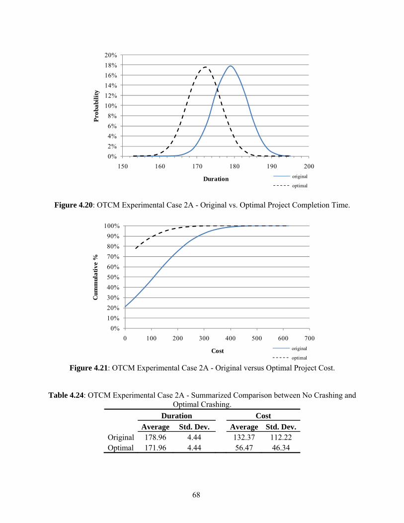
68
0%2%4%6%8%
10%12%14%16%18%20%
150 160 170 180 190 200
Prob
abili
ty
Duration original
optimal
Figure 4.20: OTCM Experimental Case 2A - Original vs. Optimal Project Completion Time.
0%10%20%30%40%50%60%70%80%90%
100%
0 100 200 300 400 500 600 700
Cum
mul
ativ
e %
Cost original
optimal Figure 4.21: OTCM Experimental Case 2A - Original versus Optimal Project Cost.
Table 4.24: OTCM Experimental Case 2A - Summarized Comparison between No Crashing and
Optimal Crashing. Duration Cost Average Std. Dev. Average Std. Dev. Original 178.96 4.44 132.37 112.22 Optimal 171.96 4.44 56.47 46.34

69
The 95% confidence interval on the difference of the means 50000,01µ between the average
cost of the project when no crashing is applied and the average cost of the project when the
solution provided by Phase I is implemented is:
[75.19 ≤ 50000,01µ ≤ 76.62].
In evaluating Phase II 500 instances of the project are simulated. Table 4.25 summarizes
the results of implementing the original project, Phase I, and Phase II on the 500 simulated
instances of the project.
Table 4.25: OTCM Experimental Case 2A - Summarized Comparison between Original Project, Phase I and Phase II.
Duration Cost Average Std. Dev. Average Std. Dev. Original 178.84 4.34 128.18 110.34 Phase I 171.84 4.34 55.02 44.31 Phase II 173.32 2.79 43.10 39.50
The 95% confidence interval on the difference of the means 500,01µ between the average
cost of the original project and the average cost of the project when Phase I is implemented is:
[66.02 ≤ 500,01µ ≤ 80.31].
The 95% confidence interval on the difference of the means 500,12µ between the average
cost of the project when Phase I is applied and the average cost of the project when Phase II is
implemented is:
[10.14 ≤ 500,12µ ≤ 13.68].

70
4.7.2.2 Case 2B: A Project Having 24 Activities
Case 2B considers a project network having 24 activities. A project network presented by
Haga (1998) is considered. The project network (depicted graphically in Figure 4.22) has 24
activities, there are multiple potential critical paths, and each activity is only preceded by one
activity. All the activities in the network have a crashing potential of 5 time units. The activity
times are represented by beta distributions, and the target completion time of the project is time
50. Table 4.26 shows the estimates used to fit the beta distributions representing the duration of
the activities, as well as the crashing costs and predecessors of each activity. The equation
defining the penalty cost for late completion is
⎩⎨⎧
>−≤
=50τif),50τ(4050τif,0
)τ,(TPF.
The optimal solution provided by the OTCM program is to crash activities 1 and 3 four
times each, activity 2 twice, and activity 14 once with an estimated average project cost of
203.99. Figure 4.23 and Figure 4.24 show the distribution of project completion time and the
distribution of project cost, respectively, which are generated by running 50,000 replications of
the project network. Table 4.27 summarizes the results.

71
1
2
3
4
7
6
5
8
9
12
14
13
10
11
15
17
16
20
18
22
19
21
23
24
START END
Figure 4.22: OTCM Experimental Case 2B - Project Network (Adapted from Haga 1998).

72
Table 4.26: OTCM Experimental Case 2B - Activity Duration Information, Crashing Cost, and Predecessors for Each Activity.
Activity a ml b Crash Cost Predecessors 1 10 20 30 10 - 2 20 30 40 10 - 3 10 20 30 10 - 4 10 15 20 10 1 5 10 15 20 10 1 6 10 15 20 10 1 7 10 15 20 10 1 8 10 15 20 10 1 9 10 15 20 10 4 10 10 15 20 10 5 11 10 15 20 10 6 12 10 15 20 10 7 13 10 15 20 10 8 14 17 22 27 10 2 15 10 15 20 10 3 16 10 15 20 10 3 17 10 15 20 10 3 18 10 15 20 10 3 19 10 15 20 10 3 20 10 15 20 10 15 21 10 15 20 10 16 22 10 15 20 10 17 23 10 15 20 10 18 24 10 15 20 10 19

73
0%
2%
4%
6%
8%
10%
12%
14%
16%
35 40 45 50 55 60 65 70
Prob
abili
ty
Durationoriginal
optimal
Figure 4.23: OTCM Experimental Case 2B - Original vs. Optimal Project Completion Time.
0%10%20%30%40%50%60%70%80%90%
100%
0 100 200 300 400 500 600 700
Cum
mul
ativ
e %
Cost original
optimal
Figure 4.24: OTCM Experimental Case 2B - Original versus Optimal Project Cost.
Table 4.27: OTCM Experimental Case 2B - Summarized Comparison between No Crashing and Optimal Crashing.
Duration Cost Average Std. Dev. Average Std. Dev. Original 55.68 2.70 227.59 106.57 Optimal 51.99 2.69 204.32 87.10

74
The 95% confidence interval on the difference of the means 50000,01µ between the average
cost of the project when no crashing is applied and the average cost of the project when the
solution provided by Phase I is implemented is:
[22.94 ≤ 50000,01µ ≤ 23.59].
4.7.2.3 Case 2 Discussion
The results of Case 2A indicate that Phase I provides a significant reduction in cost
relative to not crashing the project network. In addition, since there is only one critical path is
possible to verify that the solution provided by the OTCM is optimal (recall Case 1 discussion);
the crashing configuration provided by the OTCM program is to crash the activities with the
lowest crashing costs. In addition, the results show that implementing Phase II provides a
significant reduction in cost relative to implementing Phase I.
For Case 2B the results indicate that implementing the solution provided by the OTCM
program significantly improves the average project cost. Changing the number of activities of the
project network doesn’t change the type of constraints (linear) or decision variables (integer)
required by the optimization component of OTCM in order to assure optimality. Therefore, it can
be concluded that the solution provided for Case 2B is optimal. The OTCM program ran for 1.5
hours to find the Phase I optimal solution of this network, which is significantly longer than the
time it ran for to find the optimal solution for all the other examples and experiments previously
shown (the OTCM program found the solution in an average of 1 minute). This indicates that
there is a significant impact in the performance of the optimization engine used by OTCM when
the number of decision variables goes from less than 15 activities to more 20 activities. This is
consistent with the limitations of ISC, which is the optimization engine used by OTCM.

75
According to the developers of ISC, the current version of ISC is “appropriate for up to 10
decision variables and any finite number of feasible solutions” (Xu et al., 2007). Please note that
this is not a limitation of OTCM itself, but of the current stochastic optimization engine used by
OTCM. Since Phase II can be considered as multiple applications of Phase I, and given the large
amount of time it takes the OTCM program to find a solution for an evaluation of the project
network presented in Case 2B, it is not practical to run Phase II. However, an improvement in
average cost is expected from implementing Phase II.
4.7.3 OTCM Experimental Case 3
Case 3 of the experimental performance evaluation demonstrates the ability of the OTCM
method to obtain an optimal solution for projects having low or high variability in activity time.
Case 3A considers a project having low variability in activity time and Case 3B considers a
project having high variability in activity time.
4.7.3.1 Case 3A: A Project Having Low Variability in Activity Time
Case 3A considers project having low variability in activity time. Since only the effect of
the variability in activity time is being considered in this experiment, a simple network with only
one critical path is chosen for this experiment. The project network has 13 activities and is
depicted graphically in Figure 4.25. Each activity on this project has the potential to be crashed
up to 3 time units. The activity times are represented by triangular distributions. The duration
estimates used to fit the triangular distribution of each activity, as well as the crashing costs per
time unit for each activity are shown in Table 4.28. The target completion time of the project is
time 175, and the equation defining the penalty cost for late completion is

76
⎩⎨⎧
>−≤
=175τif),175τ(30175τif,0
)τ,(TPF.
1 2 3 4 765 8 9 10 11 12 13
Figure 4.25: OTCM Experimental Case 3A - Project Network.
Table 4.28: OTCM Experimental Case 3A - Minimum (a), Mode (m), and Maximum (b) Duration, and Crashing Cost for Each Activity.
Activity a m b Crash Cost 1 11.5 12 12.5 13 2 12.5 13 13.5 15 3 9.5 10 10.5 17 4 13.5 14 14.5 7 5 8.5 9 9.5 18 6 14.5 15 15.5 12 7 13.5 14 14.5 6 8 15.5 16 16.5 8 9 20.5 21 21.5 15 10 7.5 8 8.5 6 11 18.5 19 19.5 14 12 12.5 13 13.5 10 13 14.5 15 15.5 12
The optimal solution for Phase I provided by the OTCM program is to crash activity 7
three times, and activity 10 twice with an estimated average project cost of 30.87. The
distributions of project completion time and project cost are shown in Figures 4.26 and 4.27,
respectively; both distributions are generated with 50,000 data points. Table 4.29 summarizes the
results of Phase I evaluation.

77
0%
5%
10%
15%
20%
25%
30%
35%
40%
45%
168 173 178 183
Prob
abili
ty
Duration original
optimal
Figure 4.26: OTCM Experimental Case 3A - Original vs. Optimal Project Completion Time.
0%10%20%30%40%50%60%70%80%90%
100%
0 25 50 75 100 125 150 175 200
Cum
mul
ativ
e %
Cost original
optimal
Figure 4.27: OTCM Experimental Case 3A - Original versus Optimal Project Cost.
Table 4.29: OTCM Experimental Case 3A - Summarized Comparison between No Crashing and Optimal Crashing.
Duration Cost Average Std. Dev. Average Std. Dev. Original 178.99 0.74 119.78 22.19 Optimal 173.99 0.74 30.86 3.73
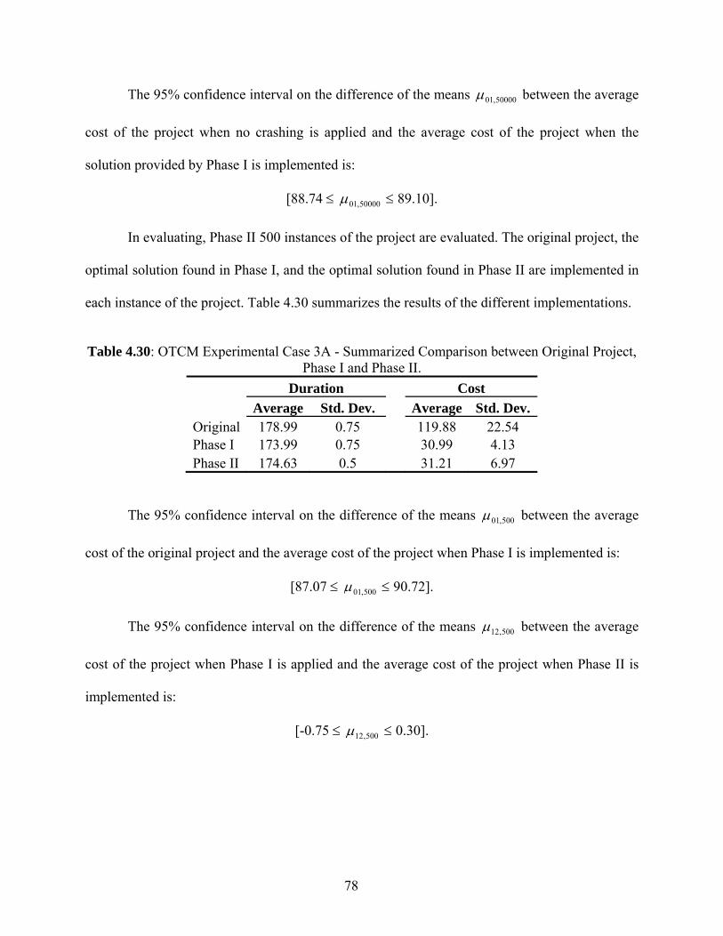
78
The 95% confidence interval on the difference of the means 50000,01µ between the average
cost of the project when no crashing is applied and the average cost of the project when the
solution provided by Phase I is implemented is:
[88.74 ≤ 50000,01µ ≤ 89.10].
In evaluating, Phase II 500 instances of the project are evaluated. The original project, the
optimal solution found in Phase I, and the optimal solution found in Phase II are implemented in
each instance of the project. Table 4.30 summarizes the results of the different implementations.
Table 4.30: OTCM Experimental Case 3A - Summarized Comparison between Original Project,
Phase I and Phase II. Duration Cost Average Std. Dev. Average Std. Dev. Original 178.99 0.75 119.88 22.54 Phase I 173.99 0.75 30.99 4.13 Phase II 174.63 0.5 31.21 6.97
The 95% confidence interval on the difference of the means 500,01µ between the average
cost of the original project and the average cost of the project when Phase I is implemented is:
[87.07 ≤ 500,01µ ≤ 90.72].
The 95% confidence interval on the difference of the means 500,12µ between the average
cost of the project when Phase I is applied and the average cost of the project when Phase II is
implemented is:
[-0.75 ≤ 500,12µ ≤ 0.30].

79
4.7.3.2 Case 3B: A Project Having High Variability in Activity Time
Case 3B considers a project having high variability in activity time. A project network
with only one critical path is considered for this case. The project network has 13 activities and is
depicted graphically in Figure 4.28. The maximum crashing potential of each activity in this
project is 3 time units. The activity times are represented by triangular distributions. The duration
estimates used to fit the triangular distributions, and the crashing costs per time unit for each
activity are shown in Table 4.31. The target completion time of the project is time 185, and the
equation defining the penalty cost for late completion is
⎩⎨⎧
>−≤
=185τif),185τ(30185τif,0
)τ,(TPF.
1 2 3 4 765 8 9 10 11 12 13
Figure 4.28: OTCM Experimental Case 3B - Project Network.
Table 4.31: OTCM Experimental Case 3B - Minimum (a), Mode (m), and Maximum (b) Duration, and Crashing Cost for Each Activity.
Activity a m b Crash Cost 1 6 12 18 15 2 7 13 19 12 3 4 10 16 15 4 8 14 20 9 5 13 19 25 8 6 9 15 21 11 7 8 14 20 7 8 10 16 22 6 9 15 21 27 11 10 12 18 24 8 11 13 19 25 6 12 7 13 19 12 13 9 15 21 14

80
The optimal solution identified by the OTCM program is to crash the following activities
three time units each: 4, 5, 7, 8, 10, and 11. Figures 4.29 and 4.30 depict the distribution of
project completion time and project cost, respectively. Each distribution is generated using
50,000 data points. Table 4.32 summarizes the result of this evaluation.
0%2%4%6%8%
10%12%14%16%18%20%
140 160 180 200 220 240
Prob
abili
ty
Duration original
optimal
Figure 4.29: OTCM Experimental Case 3B - Original vs. Optimal Project Completion Time.
0%10%20%30%40%50%60%70%80%90%
100%
0 200 400 600 800 1000 1200 1400 1600
Cum
mul
ativ
e %
Cost original
optimal
Figure 4.30: OTCM Experimental Case 3B - Original versus Optimal Project Cost.

81
Table 4.32: OTCM Experimental Case 3B - Summarized Comparison between No Crashing and Optimal Crashing.
Duration Cost Average Std. Dev. Average Std. Dev. Original 198.91 8.88 424.18 252.71 Optimal 180.91 8.88 188.10 112.32
The 95% confidence interval on the difference of the means 50000,01µ between the average
cost of the project when no crashing is applied and the average cost of the project when the
solution provided by Phase I is implemented is:
[234.52 ≤ 50000,01µ ≤ 237.65].
The results of the evaluation of 100 instances of the project, implementing the original
project, Phase I, and Phase II are summarized in table 4.33.
Table 4.33: OTCM Experimental Case 3B - Summarized Comparison between Original Project, Phase I and Phase II.
Duration Cost Average Std. Dev. Average Std. Dev. Original 198.12 9.52 403.03 269.37 Phase I 180.12 9.52 188.32 111.25 Phase II 182.10 4.94 148.19 90.22
The 95% confidence interval on the difference of the means 100,01µ between the average
cost of the original project and the average cost of the project when Phase I is implemented is:
[175.90 ≤ 100,01µ ≤ 253.50].
The 95% confidence interval on the difference of the means 100,12µ between the average
cost of the project when Phase I is applied and the average cost of the project when Phase II is
implemented is:
[29.68 ≤ 100,12µ ≤ 50.57].

82
4.7.3.3 Case 3 Discussion
For Case 3A the optimal solution provided by Phase I was expected since there is only 1
critical path and activities 7 and 10 are the ones with the lowest crashing cost. The project cost
when Phase I is implemented is significantly smaller than the project cost when no crashing is
applied. There is no significant difference in the project cost between implementing Phase I or
Phase II. This result indicates that since the variability in activity time is so small the optimal
solution found in Phase I remains valid throughout the entire project. As it was stated in section
4.4, Phase II is implemented to take into consideration the reduction in uncertainty, which occurs
as the result of activities being completed, and that may have an impact over the optimal
crashing configuration found in Phase I. In this case, the low variability of the activity times
didn’t have an impact over the solution of Phase I.
For Case 3B implementing Phase I represents a significant reduction in project cost with
respect to not crashing the project network. Also, the project cost when Phase II is implemented
is significantly smaller than when Phase I is. The OTCM method provided an optimal solution
even when the variability in activity time was high; however, the run time increased significantly
with respect to the case when the variability was low. The run time of OTCM when solving
Phase I of Case 3A was 17 seconds, whereas the run time when solving Phase I of Case 3B was
1,104 seconds (18.4 minutes). These results indicate that OTCM is consistent in providing an
optimal solution but that the high variability in activity times makes the optimization problem
harder to solve.

83
4.7.4 Summary of Experimental Performance Evaluation
In the three experimental cases the OTCM method is shown to be effective in identifying
the optimal crashing configuration that results in the minimum expected total cost. Thus, the
experimental performance evaluation shows that the OTCM method can consistently and
robustly provide the optimal crashing configuration of traditionally defined crashing problems.
4.8 Summary of OTCM
The OTCM is designed to provide an optimal solution to the traditionally defined
stochastic time-cost tradeoff problem. The OTCM method is designed to be implemented in two
phases; Phase I is implemented prior to the start of the project, and Phase II is implemented
throughout the project. The OTCM program, which contains the simulation model representing
the project network to be solved and the stochastic optimization engine, is used in each phase to
find an optimal solution. An experimental performance evaluation is conducted to investigate the
ability of the OTCM to consistently provide optimal crashing configurations for Phase I and
Phase II; the results of the evaluation indicate that the OTCM method is robust and consistently
provide optimal solutions. In order to facilitate the implementation of the OTCM, the OTCM
program and the OTCM project simulator are integrated into Microsoft Project. The details about
the integration are presented in Chapter 6. The methods developed for the generalized time-cost
tradeoff problem are presented in chapter 5.
84
5. DYNAMIC SELECTION OF ACTIVITY ALTERNATIVES
In the previous section methods to obtain optimal crashing configurations under
uncertainty are introduced. Although these methods are robust and provide optimal solutions,
they are designed to solve the traditionally defined stochastic time-cost tradeoff problem. This
section presents simulation-based methods to solve the generalized stochastic time-cost tradeoff
problem, which may more accurately represent the situations that a project manager might
encounter when managing a project.
Within the context of this research, the generalized stochastic time-cost tradeoff problem
is defined as follows. Given a project defined by individual activities, their precedence
relationships, and stochastic activity durations, a network representing the project can be
developed. An example of such a project (DSA Sample Project) having 4 activities is described
in Table 5.1 (Figure 5.1 depicts graphically the project network). The activities that make up a
project may have several alternatives each with an associated cost and stochastic duration. The
alternatives of an activity might include working over time, bringing in additional resources, or
subcontracting the work. The alternative potential of an activity is the number of alternatives
associated with the activity. In the generalized definition of the time-cost tradeoff problem, the
costs associated with implementing the alternatives of an activity can be independent from each
other. Table 5.1 shows the different alternatives of each activity on the DSA Sample Project
along with their associated cost. For the first activity in the example the alternative potential is
assumed to be 0, because the activity must be completed using the current available resources
(this alternative is referred to as base alternative). For each one of the remainder activities there
are 2 contractors available that can be hired to complete the work for an additional cost. If the
project is late, a lateness penalty is assessed as a linear function of the quantity of time by which

85
the project is late. For example, a project that is due at time 65 with a lateness penalty of 100 per
time unit would have the following penalty function,
⎩⎨⎧
>−≤
=65τif),65τ(10065τif,0
)τ,(TPF.
Note that the notation used throughout Chapter 5 to describe the different probability
distribution used to represent activity duration is as follows:
• Triangular Distribution: T min mode max
• Beta Distribution: B min mode max
• Uniform Distribution: U min max
• Exponential Distribution: E mean
• Constant: C constant
Solving the generalized stochastic time-cost tradeoff problem means to determine the
appropriate alternative for each activity in order to minimize the average project total cost, where
the total cost is defined as the penalty due to lateness plus the costs of the alternatives selected.
Table 5.1: DSA Sample Project Specifications. Alternative Cost
Activity Base 1 2 1 2 Predecessors1 T10 15 20 - - - - - 2 T10 20 30 U15 30 U10 20 10 30 1 3 T15 20 25 T7 8 9 E13 25 15 2 4 U13 19 T11 13 15 U10 28 10 10 3
1 2 3 4
Figure 5.1: DSA Sample Project Network.

86
The purpose of this stage of the research is to develop static and dynamic simulation-
based analysis methods for the generalized stochastic time-cost tradeoff problem capable of
evaluating project networks to answer the following questions:
• Which activity alternatives should be chosen in order to minimize the average project
cost?
• Should the configuration of alternatives be changed throughout the project?
The method presented in this section is named Dynamic Selection of Activity
Alternatives (DSA). The DSA method is designed to be implemented in two phases. Phase I
evaluates the project prior to its start taking into account all the uncertainty associated with the
duration of the activity alternatives, and provides the configuration of alternatives that minimizes
the project cost with respect to the information available. During Phase II, which is applied as the
project progresses, dynamic reevaluations of the project are performed in order to consider the
known durations (and sunk costs) of completed activities and the effect of the uncertainty of the
durations of the remaining activity alternatives, and to determine the configuration of alternatives
to be implemented from that point forward.
The current version of the DSA method is a heuristic. DSA is designed to address a
problem where there might not be a linear relationship between the costs of the alternatives
associated with any activity; since the optimization engine currently incorporated into DSA, has
some linearity requirements to assure optimality, it is not possible to guarantee that DSA will
always provide an optimal solution. However, if a simulation-based optimization procedure is
designed to address the specific type of problems DSA is solving, it could be incorporated into
DSA and optimality guarantees could be made.

87
In the next sections, Phase I and Phase II of the DSA method are presented. Although the
two phases are designed to be used together to maximize the benefit of the method, Phase I can
be applied independently from Phase II at the start of the project with Phase II being optional.
5.1 Assumptions Considered in the DSA Method
The DSA method is designed taking the following assumptions:
1) Activity times are independent;
2) Each activity has a base alternative and the stochastic duration associated with it
corresponds to the time it takes to complete the activity with the current available
resources. Each activity may also have additional alternatives, each one with an
associated stochastic duration and cost;
3) The stochastic duration of an alternative can be represented with a probability distribution
having a smaller mean and/or variance than the probability distribution representing the
duration of the base alternative;
4) The stochastic durations associated with the alternatives of a given activity don’t need to
be represented by the same type of probability distribution, i.e. the stochastic duration of
one alternative might be represented by an exponential distribution, and another one
might be represented by a triangular distribution;
5) Activity time distributions can be estimated using any probability distribution. However,
for this research only the following probability distributions are considered: beta,
triangular, exponential, and uniform;
6) The cost of implementing each activity alternative is known or can be estimated very
accurately;

88
7) For any activity, the cost of implementing the base alternative is not necessarily smaller
than the cost of implementing one of the other alternatives;
8) The costs associated with the alternatives of a given activity may be independent (i.e., not
having any type of relationship among them, such as a linear one);
9) Penalty costs for late completion, represented by a linear function, are defined before the
start the project; and
10) Precedence constraints are assumed to be strictly defined (a successor activity cannot
begin until all the predecessors have been completed).
Note that although the cost of implementing the base alternative of an activity doesn’t
need to be smaller than the cost of the other alternatives, the examples and experiments presented
in this thesis are designed assuming the base alternative is the one with the lowest cost.
5.2 DSA Phase I: Selection of Alternatives Prior to the Start of the Project
The objective of Phase I of the DSA method is to obtain the optimal configuration of
alternatives prior to the start of the project that will minimize the expected total project cost due
to lateness penalties and costs of the activity alternatives selected. Since Phase I is implemented
before the project starts, all the uncertainty associated with the completion time of the
alternatives of each activity is considered. The uncertainty is represented by probability
distributions.
Phase I involves the following steps:
• Defining the project in terms of the activities, predecessors, alternatives of each activity
with their associated stochastic durations and costs, and the penalty cost function;
• Constructing a simulation model of the project network;

89
• Utilizing a stochastic simulation optimization tool such as Industrial Strength COMPASS
(ISC) to determine the optimal configuration of alternatives;
• Evaluating the effect of selecting the base alternative for each activity in the project and
the effect of implementing the configuration of alternatives provided by DSA Phase I,
using the DSA project simulator;
• Implementing the optimal configuration of alternatives; and
• Proceeding to Phase II (optional).
The first step of the process is to specify the parameters that define the project network
and the optimization problem. The parameters include the number of activities, the probability
distribution associated with the duration of the alternatives of each activity, the predecessors of
each activity, the maximum completion time by which no penalties are applied, and the cost of
implementing the different alternatives of each activity.
A simulation model of the project network is constructed after the input parameters are
provided. The simulation model represents all the activities in the project and the precedence
relationships that exist among them. The model is used to evaluate the various configurations of
alternatives that could be implemented in the project. Evaluating a configuration of alternatives
involves running a specified number of replications (instances) of the project network, under the
configuration of alternatives that is being considered, in order to estimate the average project
cost resulting from that configuration. Running a replication of the simulation model
representing the project network involves sampling an activity time from the probability
distribution representing the duration of the alternative selected for each activity, calculating the
start time and completion time of each activity taking into account that precedence relationships
must be enforced, calculating the completion time of the project, calculating the penalty for late

90
completion (if any), and finally computing the project cost, which consists of the lateness penalty
and the cost of the activity alternatives selected.
After defining the simulation model of the project network, and determining the
alternatives of each activity, it is time to run the optimization program (DSA program). The type
of simulation-based optimization engine for the DSA method should have the capability to
optimize the expected value of simulation-generated performance measure, which is dependent
upon a set of integer decision variables. In addition, the optimization engine must not require a
linear relationship between the magnitude of the effect associated with the values that a
particular integer decision variable can take; i.e. if increasing the value of an integer decision
variable from 1 to 2 increases the magnitude of the performance measure by 5 units, increasing
the value of the same decision variable from 2 to 3 may or may not increase the magnitude of the
performance measure by 5. In any case, the optimization engine should be expected to produce
an optimal solution within certain precision specified by the user. The optimization engine
searches the solution space for potential optimal solutions. Once a potential solution (set of
activity alternatives) is found it is sent to the simulation model for evaluation. The simulation
model runs a specified number of instances of the project for the configuration of activity
alternatives sent by the optimization engine and calculates the cost of the project in each
instance; the number of instances to be evaluated is determined by the optimization engine. The
elements of the cost are the penalty due to lateness (generated by a linear penalty function), and
the sum of costs of the alternatives selected. The cost of the evaluated instances of the project is
sent to the stochastic optimization engine which tests the configuration for optimality. The
optimization engine continues the evaluation of potential solutions until the optimal solution has
been identified. At that point, the optimal solution is reported, which includes the configuration

91
of activity alternatives that minimizes the average project cost and statistics associated to this
configuration, such as sample mean of project cost, sample mean of project variance, and a 95%
confidence interval on project cost.
After obtaining the optimal solution, the DSA project simulator is used to evaluate the
impact that implementing the original (choosing the base alternative for each activity) or the
DSA configuration of alternatives has on the average project cost. The output of the project
simulator includes statistics about the project completion time and project cost (sample mean,
sample variance, and a 95% confidence interval), and provides the data required to plot the
distributions of project completion time and project cost under both configurations of alternatives
(original vs. DSA). Using these pieces of information, the project manager can decide if the
optimal configuration of alternatives will be implemented. The project manager also decides if
Phase II will be applied.
5.3 DSA Phase I Example
To illustrate Phase I of the DSA method, the DSA Sample Project discussed in the
introduction of Chapter 5 is used. The details are shown again for convenience in Table 5.2 and
Figure 5.2. In this example, the project network consisting of 4 activities has only one critical
path. The first activity can only be performed using the resources currently assigned to it, but for
each one of the remainder activities there are two contractors available to perform the work. The
stochastic duration and associated cost of each alternative is shown in Table 5.2. This is
considered to be a critical project and late completion is heavily penalized. The target completion
time of the project is time 65, and the equation defining the penalty cost for late completion is
⎩⎨⎧
>−≤
=65τif),65τ(10065τif,0
)τ,(TPF

92
where τ is the resulting completion time of the project. Figure 5.3 illustrates the input file used to
run the DSA method.
Table 5.2: DSA Phase I Example - Project Specifications. Alternative Cost
Activity Base 1 2 1 2 Predecessors1 T10 15 20 - - - - - 2 T10 20 30 U15 30 U10 20 10 30 1 3 T15 20 25 T7 8 9 E13 25 15 2 4 U13 19 T11 13 15 U10 28 10 10 3
1 2 3 4
Figure 5.2: DSA Phase I Example - Project Network.
The solution provided by DSA indicates that activities 1 and 2 are to be performed using
the current resources assigned to them, and that the work required by activities 3 and 4 is to be
completed by a contractor (specifically, the solution recommends choosing the contractor
represented by alternative number 1), resulting in an estimated average project cost of 38.30 and
an associated project cost variance of 733.20 (the DSA program ran 52,160 replications to
compute these estimates). The 95% confidence interval on the average project cost when the
solution provided by Phase I is implemented is:
[38.07 ≤ 0µ ≤ 38.54].
The original project as well as the project using the DSA solution are simulated 50,000 times to
generate the distribution of completion time (Figure 5.4) and the cumulative distribution of
project cost (Figure 5.5). Table 5.3 summarizes the results of this evaluation.

93
n 4
T 65
P 100
SC 0
NPi 0 1 1 1
0 1 2 3
APi 0 2 2 2
Distribution T10 15 20 Of Duration T10 20 30 U15 30 U10 20 Of Activity T15 20 25 T7 8 9 E13 Alternatives U13 19 T11 13 15 U10 28 (Aij)
0 Cost of 0 10 30 Alternative 0 25 15 (CAij) 0 10 10
ISC output Parameters 10000000 1 0 -1 -1 0 -1 1 -1 -1 -1 0.01 -1 0.01 0.5 50 10 0 50
Figure 5.3: DSA Phase I Example - Input File.
0%
2%
4%
6%
8%
10%
12%
14%
16%
18%
30 40 50 60 70 80 90 100
Prob
abili
ty
Duration original
DSA
Figure 5.4: DSA Phase I Example - Original versus DSA Project Completion Time.
Predecessors (PMij = 1 for each j in row i, i = 1,…,n)

94
0%10%20%30%40%50%60%70%80%90%
100%
0 500 1000 1500 2000 2500 3000
Cum
mul
ativ
e%
Cost original
DSA
Figure 5.5: DSA Phase I Example - Original versus DSA Project Cost.
Table 5.3: DSA Phase I Example - Summarized Comparison between Original Project and DSA Solution.
Duration Cost Average Std. Dev. Average Std. Dev. Original 70.97 5.29 631.10 473.09 DSA Phase I 55.97 4.66 38.19 26.49
Using paired data the 95% confidence interval on the difference between the average
project cost of the original project and the project with DSA Phase I configuration of alternatives
implemented is constructed:
[588.82 ≤ 50000,01µ ≤ 596.99] .
The results indicate that there is an impressive reduction in the project cost when the
configuration of alternatives recommended by DSA is implemented. The cost of the contractors
chosen for activities 3 and 4 is 35. Table 5.2 indicates that the average project cost when the
DSA solution is applied is 38.19; therefore, the penalty cost when the DSA solution is
implemented is in average 3.19.

95
5.4 DSA Phase II: Dynamic Selection of Alternatives during the Project Execution
In Phase I, prior to the start of the project an initial configuration of alternatives is
obtained by analyzing the entire project network. This initial optimal configuration considers the
uncertainty associated with the duration of all the alternatives associated with all the activities of
the project. As activities are completed, the uncertainty associated with their duration is
eliminated. Thus the overall uncertainty about the project completion time is reduced; as a result
the initial solution might change. The purpose of DSA Phase II is to determine the optimal
configuration of alternatives for the remaining activities.
In addition to the general assumptions of the DSA method, the following assumptions are
applied to Phase II:
• The reevaluation points occur just prior to starting an activity that has been previously
recommended to be completed not using the base alternative. The initial reevaluation
points are assumed as the start times of the activities that are specified to use an
alternative other than the base alternative, as identified in Phase I;
• The remaining time for activities in progress is known or can be estimated very
accurately; and
• The resources required to implement an activity alternative are available at the moment
of making the decision of choosing the alternative.
Due to the first assumption, Phase II is a heuristic (even when an optimization engine
capable to guarantee an optimal solution for the type of problem that the DSA method solves is
used). In order for Phase II to be optimal throughout the project, the project network should be
constantly evaluated. Constantly evaluating the project is not practical and cost prohibitive, thus,
in this research it has been assumed that the project is reevaluated when the start time of an

96
activity identified to be completed with an alternative other than the base is encountered (the
intention of the reevaluations in this case is to verify if the activity still needs to be completed
using the alternative previously selected). In addition, the first assumption indicates that if the
base alternative should be selected for all activities, according to the solution provided by Phase
I, there is no need to implement Phase II. However, although not tested here the project manager
could decide implementing Phase II at any time after the start of the project in order to determine
if choosing one of the additional activity alternatives makes economic sense due to the duration
of activities previously completed, or as changes are made to the project plan.
After the project begins, the following steps make up the dynamic method:
1. Updating the project information to reflect the current status of the project;
2. Updating the simulation model of the project network;
3. Reevaluating the remaining project network using the DSA program (as described in
Phase I) once the first activity that requires the use of an alternative other than the base
one, as identified by Phase I or a previous reevaluation, is encountered;
4. Evaluating the effects of implementing the previous configuration of alternatives and the
new DSA Phase II configuration of alternatives using the DSA project simulator; and
5. Implementing the project network under the new configuration of alternatives and
continue until either:
a) the next activity that requires the use of an alternative other than the base is
encountered and go to step 1; or
b) the project is complete.
For each iteration of Steps 1-4 of the Phase II of the DSA procedure, a new configuration
of alternatives for the remainder of the project will be identified that takes into account the sunk

97
activity times and costs associated with the activities in progress and the activities that have been
completed. If during a dynamic reevaluation it is determined that the alternative planned to be
used for a specific activity should be changed, there might be an additional “switching cost”
associated with the new alternative as a consequence of making the change. The switching cost
might be included in the reevaluation process by adding it to the predefined cost of implementing
the alternatives.
The first step in the procedure that Phase II follows is to update the information that
defines the current status of the project. For the activities completed or in progress, their
alternative potential is set to 0 and their duration is represented by their actual/estimated duration
(instead of by a probability distribution). For each activity that hasn’t started the alternative
potential, the stochastic duration of its alternatives, and the cost of implementing the alternatives
are considered to be equal to the ones used in Phase I. Also, Phase II considers the same target
completion time and the same penalty function used in Phase I (note that since the project
information is updated before each reevaluation it is possible to include information different
than the one provided in Phase I or in previous Phase II reevaluations). The updated information
is input into the simulation model to guarantee that the simulation model is an accurate
representation of the project network.
After the simulation model is updated the optimization process, as described in Phase I, is
applied. Then, the configuration of alternatives provided by the DSA program and the previous
configuration of alternatives are evaluated with the DSA project simulator. As in Phase I, the
project manager uses the output of the DSA project simulator to decide whether or not to
implement the solution provided by the Phase II reevaluation. This process continues until
another reevaluation point is encountered or until the project is complete.

98
5.5 DSA Phase II Example
The DSA Sample Project used to illustrate Phase I is now used to demonstrate Phase II of
the DSA method. Recall that the DSA Sample Project has 4 activities and only one critical path
(the details about the project and the corresponding project network are shown in Table 5.2 and
Figure 5.2). The solution provided by DSA in the Phase I indicates that for activities 3 and 4 a
contractor should be used. Given this information, the project can begin. (Although not occurring
in this example, if any of the activities that start at the project starting time are recommended by
Phase I not to use the base alternative, the recommended alternative should be implemented
without the reevaluating the project network first.) To facilitate a direct comparison among
project implementations using the base alternative for each activity, the result of DSA Phase I
only, and the full implementation of the DSA method (Phases I and II), one instance of the DSA
Sample Project is simulated. The resulting activity times for all the alternatives are shown in
Table 5.4.
Table 5.4: DSA Phase II Example - DSA Sample Project Instance. Alternative Cost
Activity Base 1 2 1 2 1 17.48 - - 2 21.23 18.68 11.08 10 30 3 22.21 8.02 3.64 25 15 4 16.52 12.23 12.01 10 10
After the project begins, the DSA Phase II procedure specifies that the project
reevaluation points (the points at which the configuration of alternatives is reevaluated) will
occur just prior to starting activities that have previously been identified by the DSA method not
to use the base alternative. In the DSA Sample Project, at time 38.71 which corresponds to the
completion time of activity 2, the first activity that Phase I specified to use an activity alternative

99
different than the base one is encountered. Consequently, the time just prior to the start of
activity 2 will serve as the reevaluation point. Figure 5.6 depicts the status of the project up to the
first reevaluation point.
Legend:Completed & Base Duration
In process & Base Duration
Completed & Alternative Duration
In process & Alternative Duration
Not Started
Evaluation Point
3 41 2
Figure 5.6: Network Status by First Reevaluation Point – DSA Phase II Example.
To implement the reevaluation, the DSA program is invoked with an input file that
reflects the current project status. This input file is shown in Figure 5.7. The bold entries indicate
the updates required from the initial DSA Phase I implementation. (Note that in this DSA
Sample Project, the alternative potential for each of the remaining activities remains the same
throughout the project. However, any changes to the project parameters including the alternative
potential, the duration of the activity alternatives and their associated cost can be updated at any
time and included in the reevaluation.) Thus, the updates to the input file needed for this
reevaluation include changing the alternative potential of activity 2 to 0 and entering the actual
durations of activities 1 and 2 as constant times of 17.48 and 21.23, respectively.

100
n 4
T 65
P 100
SC 0
NPi 0 1 1 1
0 1 2 3
APi 0 0 2 2
Distribution C17.48 Of Duration C21.23 Of Activity T15 20 25 T7 8 9 E13 Alternatives U13 19 T11 13 15 U10 28 (Aij)
0 Cost of 0 Alternative 0 25 15 (CAij) 0 10 10
ISC output Parameters 10000000 1 0 -1 -1 0 -1 1 -1 -1 -1 0.01 -1 0.01 0.5 50 10 0 50
Figure 5.7: DSA Phase II Example - Input File First Reevaluation.
Upon running the DSA program, a new configuration of alternatives is obtained for the
remaining activities. Table 5.5 shows the resulting configuration of alternatives which specifies
that activity 3 is to be completed using the first contractor (this in consistent with the result of
Phase I), and that activity 4 is to be completed with the resources originally assigned to it (rather
than using the services of a contractor as specified by Phase 1). Table 5.6 indicates the new
estimate of the average project cost (Sample Mean of Cost) and the associated estimate of the
project cost variance (Sample Variance of Cost) which are 30.54 and 362.27, respectively. In
addition, the number of simulated instances of the project used to obtain the estimates, 519,333
replications, is also listed.
Predecessors (PMij = 1 for each j in row i, i = 1,…,n)

101
Table 5.5: DSA Phase II Example - Configuration of Alternatives Provided by First Reevaluation.
Activity 1 2 3 4
Alternatives 0 0 1 0
Table 5.6: DSA Phase II Example - Summary of Solution Provided by First Reevaluation. Replications 519,333
Sample Mean of Cost 30.54 Sample Variance of Cost 362.27
Upon implementing the specified configuration of alternatives the project proceeds
without finding any reevaluation point and reaches its end. The cost of using a contractor to
complete activity 3 is 25. The resulting completion time of the project is 63.25; therefore, there is
no penalty due to lateness and the total cost of this instance of the project is 25.
Table 5.7 shows the configuration of alternatives provided by both Phase I and Phase II.
If only Phase I is implemented the project completion time is 58.97; therefore, a penalty cost is
avoided and the total cost of the project is 35, resulting from choosing contractors for activities 3
and 4. If the original project is implemented the completion time of the project is 77.45, resulting
in a very high project cost of 1,244.95. Table 5.8 presents a summary of these results. Since this
is a project heavily penalized for late completion and the configurations provided by Phase I and
Phase II result in an on-time completion of the project, a large reduction in project cost is
achieved. Implementing only Phase I resulted in a 97% reduction in the total project cost, and
implementing the Phase II resulted in a 98% reduction in the total project cost.
Table 5.7: DSA Phase II Example – Configurations of Alternatives Provided by Phase I and Phase II.
Activity Phase 1 2 3 4
Phase I 0 0 1 1 Phase II 0 0 1 0

102
Table 5.8: DSA Phase II Example - Original vs Phase I vs Phase II. Cost
Phase Completion time Alternatives Penalty Total Original 77.45 0 1,244.95 1,244.95 Phase I 58.97 35 0 35 Phase II 63.25 25 0 25
To provide statistical support about the benefit of implementing Phase II over just
implementing Phase I, 500 instances of the project are simulated and their results are used to
build a 95% confidence interval on the difference between (paired observations) the average cost
of the project when Phase I is implemented and the project when the Phase II is implemented:
[8.87 ≤ 500,12µ ≤ 10.82].
The results indicate that implementing Phase I has a higher cost than implementing Phase II.
5.6 DSA Optimization Program and DSA Project Simulator
The optimization program used in Phase I and Phase II of the DSA method to obtain an
optimal configuration of alternatives has three main components: the input file, the DSA
program containing the simulation model and the optimization engine, and the output files
containing the performance measures of the solution identified. The interaction between the
components of the optimization program, which is the same for Phase I and Phase II, is shown in
Figure 5.8. The difference between Phase I and Phase II, with respect to the optimization
program, is in the input and the DSA program which considers in Phase II the portion of the
project that has been completed and the associated sunk costs, and optimizes the configuration of
alternatives for the remainder of the project.

103
PROJECT PARAMETERS
(n, Aij, PM, T, P, APi, CAij,SC)
OPTIMIZATION ENGINE
Minimizes.t.xi ≤ APi ∀i = 1,…,n
SIMULATION MODEL
C = PF(T , τ) + + SC
x
C
OPTIMAL CONFIGURATIONOF ALTERNATIVES
- Sample Mean of Project Cost- Sample Variance of Project Cost
- 95% CI on Project Cost
Input File
Output Files
DSA Program
Figure 5.8: Components of the DSA Optimization Program.
As part of the DSA procedure, once a solution is identified the DSA project simulator is
used to compare the impact that implementing the new configuration of alternatives or the
previous configuration of alternatives has on the average project cost and the average project
completion time. The DSA project simulator has the following components: the input file, the
simulation model, and the output file containing statistics about the project cost and the project
C∑=
n
iixi
CA1

104
completion time for each one of the configurations evaluated. Figure 5.9 depicts the interaction
between the components of the DSA project simulator.
PROJECT PARAMETERS
(n, Aij, PM, T, P, CAij, SC, x)
CURRENT & DSA CONFIGURATIONS OF
ALTERNATIVES
- Sample Mean of Project Cost & Duration
- Sample Variance of Project Cost & Duration
- 95% CI on Project Cost & Duration- Distribution of Project Cost &
Duration
SIMULATON MODEL
Input File
Output Files
Figure 5.9: Components of the DSA Project Simulator.
A detailed explanation about the components of the DSA optimization program and the
DSA project simulator is presented in the next sections.

105
5.6.1 DSA - Input Files
The input file of the DSA optimization program includes the following information:
• First line: number of activities in the project (n);
• Second line: target completion time (T);
• Third line: penalty cost per unit of lateness (P);
• Fourth line: sunk cost (SC);
• Fifth line: number of predecessors per activity (NPi ∀i = 1,…,n);
• Next n lines: predecessors of activity (PMij = 1 for each j in row i, i = 1,…,n);
• Next line: alternative potential for activity i (APi ∀i = 1,…,n);
• Next n lines: distribution of duration for alternatives of activity i = 1,…,n;
• Next n lines: cost of the alternatives of activity i = 1,…,n;
• Next line: name of the output file to be generated by the optimization engine (ISC); and
• Next line: parameters required by the optimization engine (ISC).
The input file of the DSA project simulator requires the following information:
• First line: number of activities in the project (n);
• Second line: target completion time (T);
• Third line: penalty cost per unit of lateness (P);
• Fourth line: sunk cost (SC);
• Fifth line: number of predecessors per activity (NPi ∀i = 1,…,n);
• Next n lines: predecessors of activity (PMij = 1 for each j in row i, i = 1,…,n);
• Next n lines: distribution of duration of the alternative of activity i to be evaluated
i = 1,…,n; and

106
• Next n lines: cost of the alternative of activity i to be evaluated i = 1,…,n.
5.6.2 DSA - Simulation Model
The simulation model used in the DSA program and in the DSA project simulator is
created in the C++ programming language. The simulation model is created in this programming
language to facilitate its interaction with Industrial Strength COMPASS (also developed in C++),
which is the optimization engine chosen for this research. The simulation model is used to
determine the expected project duration and the expected project cost (cost of alternatives plus
penalty cost); the latter represents the objective function of the optimization.
In order to define the project network to be represented by the simulation model it is
necessary to capture relevant information about the project. The following constants are created
for that purpose:
n ≡ number of activities in the project.
Aij ≡ distribution of the duration of alternative j for activity i ∀i = 1,…,n and
∀j = 1,…,APi.
S ≡ set of completed or in process activities (in Phase I, S = {∅}).
R ≡ set of remaining activities (in Phase I, R includes all project activities).
PM ≡ predecessors matrix; PMij is equal to 1 if activity i is preceded by activity j, 0
otherwise, ∀i,j = 1,…,n,
PM =
⎥⎥⎥⎥⎥⎥
⎦
⎤
⎢⎢⎢⎢⎢⎢
⎣
⎡
nnn
n
PMPM
PMPMPMPM
...................................................
......
1
21
11211
.
107
NPi ≡ number of predecessors of activity i = 1,…,n.
T ≡ target completion time.
P ≡ penalty cost per time unit of lateness.
APi ≡ alternative potential (number of alternatives) for activity i = 1,…,n, APi = 0 ∀i ∈ S.
CAij ≡ cost of alternative j of activity i ∀i = 1,…,n and ∀j = 1,…,APi.
di ≡ actual or accurately estimated duration of activity i ∈ S.
y ≡ vector of alternative selected for activity i = 1,…,n, yi ≥ 0 for i ∈ S, yi = 0 for i ∈ R.
SC ≡ sunk cost; define as the cost of the alternatives previously selected, ∑∈
=n
Siiyi
CASC .
The following variables are used in the simulation model algorithm that simulates an instance of
the project to estimate the project completion (τ) time and the project cost (C):
x ≡ vector of n integer decision variables (x = <x1, x2,…, xn>), where each decision
variable (xi) represents the alternative chosen for activity i, ∀i = 1,…,n, where xi = 0
for i ∈ S.
PCi ≡ number of predecessors of activity i already completed ∀i = 1,…,n.
ti ≡ duration for activity i = 1,…,n.
sti ≡ start time of activity i = 1,…,n.
cti ≡ completion time of activity i = 1,…,n.
ACi ≡ is set to 1 if activity i is completed, 0 otherwise, ∀i = 1,…,n.
PF(T,τ) ≡ linear function that represents the penalty for late completion.
For each replication of the simulation model (a simulated instance of the project) the
following algorithm is applied:

108
1) Set sti = cti = PCi = ACi = 0 ∀i = 1,…,n;
2) If activity i ∈ R, generate ti from Aij where j = xi; otherwise ti = di ∀i = 1,…,n;
3) Set index i = 1;
4) If ACi = 0 and PCi = NPi go to step 5, otherwise go to step 9;
5) If PMij = 1, sti = max(sti,ctj) ∀j = 1,…,n;
6) Set cti = sti + ti;
7) If PMji = 1, PCj = PCj + 1 ∀j = 1,…,n;
8) Set ACi = 1; if ∑=
=n
ii nAC
1 go to step 10;
9) If i = n, set i = 1; otherwise i = i + 1; go to step 4;
10) Set τ = max(cti ∀i = 1,…,n);
11) Set C = PF(T,τ) + ∑=
n
iixi
CA1
+ SC.
In the simulation model used by the DSA project simulator the value of xi is assigned by
the user, and in the simulation model used by the DSA program the value of xi is generated by
the optimization engine.
In order to verify the simulation model, multiple replications are run. For each
replication, the pieces of information generated by the simulation model are output and recorded.
Those pieces of information are: activity time sampled for each activity, total cost of the
alternatives selected, total penalty cost, total cost, and project completion time. Please note that
other pieces of information used to verify the simulation model such as target completion time,
configuration of alternatives applied to a particular replication, cost of each activity alternative,
and penalty cost per time unit of lateness are provided as input, thus they are available before
running each replication. All the information recorded from the replications along with the

109
information input into the simulation model is used to verify the results by hand. When verifying
each replication, the following conditions are evaluated:
• Activity time sampled for each activity felt in the range of possible values corresponding
to the probability distribution of the alternative from which the activity time is sampled.
• Activity alternatives chosen are the ones indicated in the configuration of alternatives
provided as input.
• The project completion is consistent with the sampled activity times.
• The total cost of the alternatives selected is consistent with the configuration of
alternatives and the cost of each alternative.
• Penalty cost is consistent with project completion time. If project completion time is less
or equal than the target completion time, no penalty cost is applied; if it is greater than the
target, the penalty cost increased according to the penalty cost per time unit of lateness
provided as input.
• The total project cost is the sum of the cost of the alternatives selected and the penalty
cost.
5.6.3 DSA - Optimization Engine
The simulation model uses integer decision variables that represent the activity
alternative selected for each activity; a particular set of values for these integer decision variables
represents a configuration of alternatives. The simulation model interacts with an optimization
engine with the purpose of determining the configuration of alternatives that generates the
minimum average total cost (C ). The optimization engine is responsible for selecting the
configuration of alternatives to be evaluated; for each one of these configurations of alternatives

110
the expected total cost is computed. Finally the optimization engine determines the configuration
of alternatives that minimizesC .
The optimization engine used in this step of the methodology is Industrial Strength
COMPASS (ISC) (Xu et al., 2007). ISC is a tool which is derived from the COMPASS
framework developed by Hong and Nelson (2006) for locally convergent, discrete optimization-
via-simulation (DOvS). To utilize ISC the C++ simulation model is integrated into the ISC code.
ISC requires inputs such as an initial solution, the range of possible values for each decision
variable (CPi ∀i =1,…,n), the precision within which the optimal solution is to be found (δ), and
the confidence level associated to the solution (α); these inputs must be provided in a separate
text file from which ISC reads them. ISC provides a default value for most of the input
parameters. Appendix A includes the complete list of inputs required by ISC (for additional
information about the ISC input parameters please refer to Xu et al. 2007). ISC searches the
feasible region defined by the alternative potential of the activities in the project and returns a
solution within the specified tolerance.
5.6.4 DSA - Project Simulator
The DSA project simulator has the capability to evaluate the impact that a particular
configuration of alternatives has on the project in terms of project completion time and project
cost. Although the DSA project simulator can be used to evaluate any configuration of
alternatives, it is developed with the intention of estimating time and cost statistics of the project
network when the optimal configuration of alternatives obtained in a particular evaluation of the
project network and when the previous optimal configuration of alternatives are applied. Note
that the previous configuration of alternatives considered for Phase I is usually to select the base

111
alternative for each activity, and for Phase II the previous configuration of alternatives is usually
the optimal configuration of alternatives identified at the previous reevaluation.
The complete list of inputs required by the project simulator is presented in section 5.6.1.
The outputs of the DSA project simulator include an estimate of the average project cost and the
average project completion time, an estimate of the variance of the project cost and the project
completion time, and a 95% confidence interval on the average project cost and the average
project completion time. In addition, the output includes all the data points used to calculate the
estimates, which can also be used to plot the distributions of project cost and project completion
time.
5.6.5 DSA - Integration of DSA Program Components and the DSA Project Simulator
The following algorithm summarizes the steps required by the Phase I or Phase II of the
DSA method:
Step 1: Define the project network by setting the values of n, T, P, Aij, PMij, NPi, CAij
∀i,j = 1,…,n.
Step 2: Define the optimization problem by setting the values of APi ∀i = 1,…,n, and setting
the values of the inputs required by the optimization engine such as δ and α.
Step 3: Input the simulation model into an optimization engine and solve the optimization
problem, which follows the following format:
Minimize C where C = PF(T , τ) + ∑=
n
iixi
CA1
+ SC
s.t.
xi ≤ APi ∀i = 1,…,n

112
Step 4: Run multiple replications (the number of replications is specified by the user) of the
project network using the DSA Project Simulator, implementing both the original
configuration of alternatives and the configuration of alternatives provided by DSA, to
estimate the average and the standard deviation of the project cost, to construct a
confidence interval on the average project cost, and to plot the distribution of project
cost.
5.7 DSA Experiments
To investigate the ability of the DSA method to consistently provide an optimal
configuration of alternatives, an experimental performance evaluation is conducted. In particular,
the experiments are designed to test the robustness of the DSA method to determine the optimal
configuration of alternatives in terms of minimizing the expected total cost for generalized time-
cost tradeoff problems that more accurately describe the situations that a project manager might
encounter. The DSA method relaxes the assumptions of the traditionally defined time-cost
tradeoff problems related to the way in which the alternatives of an activity and their associated
costs are represented. The experimental performance evaluation focuses on two main factors,
each one representing a different relaxation level of the assumptions.
Experimental test cases are constructed to evaluate each of the two main factors. Each
case consists of two networks, one with only one critical path and another with multiple potential
critical paths, that are used to evaluate the factors in networks of different complexity levels.
These cases are as follows:
• Case 1: Varying mean of base alternative; non-linear; ordered cost
A. A project network with a single critical path

113
B. A project network with multiple potential critical paths
• Case 2: Varying distribution of base alternative; non-linear; not-ordered cost
A. A project network with a single critical path
B. A project network with multiple potential critical paths
For each experiment, the Phase I (static) and Phase II (dynamic) DSA methods are applied and
evaluated.
To evaluate Phase I and Phase II of the DSA method, the following procedure is used.
For each factor level within each case, a project having the necessary characteristic is
selected. The projects have been arbitrarily selected to have the characteristic of interest.
The DSA Phase I and Phase II are applied to each project. The project specifications
including the stochastic duration of the activity alternatives, activity predecessors, cost of activity
alternatives, and penalty costs are specified in the input file. The input files are displayed in
Appendix C. For activities that do not require to be completed by the base alternative in each
project, the alternative potential is specified to be 2. For Phase I, the DSA program is run to
obtain the optimal configuration of alternatives that minimizes the expected total cost (cost of
alternatives plus lateness penalty cost). Finally the DSA project simulator is used to simulate
50,000 instances of the original project and the project with the DSA Phase I configuration of
alternatives implemented. The data from the 50,000 instances of each system is then used to
construct empirical graphs of the distribution of completion time and the cumulative distribution
of total cost. The estimated average and standard deviation of the project completion time and
project cost is also presented for both systems. In addition, a 95% confidence interval (using
paired data) is constructed on the difference between the mean total cost of the original project
and the project with the optimal configuration of alternatives, referred to as 50000,01µ .

114
For Phase II, the optimal configuration of alternatives obtained in Phase I is used as the
starting point for each project. Multiple instances of each project are generated. The number of
instances generated is dependent on the particular project (i.e., enough instances are generated to
identify if there is a significant difference between the average project cost when Phase I is
implemented and the average project cost when Phase II is implemented). For each project
instance, the DSA Phase II is applied. Each instance of the project is simulated selecting the base
alternative for each activity, the optimal configuration of alternatives provided by Phase I, and
the optimal configuration of alternatives provided by Phase II. The resulting completion times
and total costs under each case are recorded for each instance, and the estimated average and
standard deviation of the project cost and project completion time are presented. Finally, two
95% confidence intervals are constructed. The first confidence interval is constructed on the
difference between the average total cost of the original project and the project with the Phase I
configuration of alternatives applied, and the second confidence is constructed on the difference
between the average total cost of the project with the Phase I configuration of alternatives
applied and the project after the DSA Phase II has been applied. The confidence intervals are
referred to as N,01µ and N,12µ , respectively, where N represents the number of instances
generated for each experimental case.
In order to make the experimental process more efficient for Phase II an automated
version of the DSA method is created. This version has the following features:
• Evaluates Phase I of the network and record the optimal configuration of alternatives;
• Samples random times from Aij ∀i = 1,…,n ∀j = 1,…,APi for each instance of the project
to be used as the real duration of each activity if a particular alternative is chosen;

115
• Keeps track of the alternatives chosen by the activities completed or in progress, and their
related sunk costs;
• Determines the reevaluation points and reevaluates the network accordingly.
5.7.1 DSA Experimental Case 1
Case 1 of the experimental performance evaluation demonstrates the ability of the DSA
method to obtain an optimal solution for projects in which the assumptions considered in the
traditionally defined time-cost tradeoff problem are partially relaxed. The partial relaxation of
the assumptions considers that the duration of all the alternatives of an activity are represented
by the same type of probability distribution (beta, triangular, etc.), where the probability
distributions have the same variance but a different mean. In addition, the costs of the
alternatives are not required to have a linear relationship between them, but they must be
ordered, i.e. the alternative that reduces the activity duration the most will have the highest cost,
whereas the alternative that reduces the duration the less will have the smallest cost. Case 1A
considers a project with 1 dominant critical path and Case 1B considers a project with multiple
potential critical paths.
5.7.1.1 Case 1A: Single Critical Path; Varying Mean of Base Alternative; Non-linear; and
Ordered Costs
Case 1A considers a project with a single dominant critical path, in which the duration of
the activity alternatives is represented by a probability distribution of the same type as the one
used to represent the duration of the base alternative but with a different mean. In addition the
cost of the activity alternatives are non-linear and ordered (meaning that in the input file the

116
activity alternatives are sorted ascending by cost, and that the alternatives with the highest cost
are the ones that further reduce the duration of the activity). The project network having 7
activities is depicted graphically in Figure 5.10. Each activity has two activity alternatives
besides the base alternative. Table 5.9 shows the alternatives of each activity along with their
respective cost, as well as the precedence relationships among the activities that form the
network. The target completion time of the project is time 80, and the equation defining the
penalty cost for late completion is
⎩⎨⎧
>−≤
=80τif),80τ(3580τif,0
P
where τ is the resulting completion time of the project.
1 2 34
765
Figure 5.10: DSA Experimental Case 1A - Project Network.
Table 5.9: DSA Experimental Case 1A - Information of Activity Alternatives and Predecessors
of Each Activity. Alternative Cost
Activity Base 1 2 1 2 Predecessors1 T6 10 14 T5 9 13 T4 8 12 13 20 - 2 T5 7 9 T4 6 8 T3 5 7 5 12 1 3 T8 11 14 T5 8 11 T2 5 8 10 24 2 4 U6 10 U5 9 U4 8 5 9 3 5 T15 20 25 T13 18 23 T11 16 21 12 18 3 6 T10 20 30 T8 18 28 T6 16 26 14 32 4,5 7 U8 20 U6 18 U4 16 6 10 6
The configuration of alternatives found by DSA Phase I indicates that activities 2, and 3
should use their first alternative, and activity 7 should use its second alternative. All the other

117
activities should use their base alternative. The resulting estimated average project cost is 43.78.
The original project (all the activities with the base alternative) and the project with the DSA
configuration of alternatives are simulated 50,000 times to generate the distribution of
completion time (Figure 5.11) and the cumulative distribution of the project cost (Figure 5.12).
Table 5.10 summarizes the results of the 50,000 replications.
0%
2%
4%
6%
8%
10%
12%
14%
50 60 70 80 90 100
Prob
abili
ty
Duration original
DSA
Figure 5.11: DSA Experimental Case 1A - Original versus DSA Project Completion Time.
0%10%20%30%40%50%60%70%80%90%
100%
0 200 400 600 800 1000
Cum
mul
ativ
e%
Cost original
DSA
Figure 5.12: DSA Experimental Case 1A - Original versus DSA Project Cost.

118
Table 5.10: DSA Experimental Case 1A - Summarized Comparison between Original Project and DSA Phase I.
Duration Cost Average Std. Dev. Average Std. Dev. Original 81.97 6.14 125.44 147.83 DSA Phase I 73.97 6.14 45.30 55.06
The 95% confidence interval on the difference of the means 50000,01µ between the average
cost of the original project and the average cost of the project when the solution provided by
Phase I is implemented is:
[80.96 ≤ 50000,01µ ≤ 82.92].
In evaluating Phase II, 700 instances of the project are simulated. Each instance of the
project is simulated implementing the original project, the solution provided by Phase I, and the
solution provided by Phase II. The results are shown in table 5.11.
Table 5.11: DSA Experimental Case 1A - Summarized Comparison between Original Project,
Phase I, and Phase II. Duration Cost Average Std. Dev. Average Std. Dev. Original 81.87 6.13 122.95 150.09 Phase I 73.80 6.22 44.37 56.00 Phase II 75.23 4.74 38.03 48.42
The 95% confidence interval on the difference of the means 700,01µ between the average
cost of the original project and the average cost of the project when Phase I is implemented is:
[68.62 ≤ 700,01µ ≤ 88.55].
The 95% confidence interval on the difference of the means 700,12µ between the average
cost of the project when Phase I is applied and the average cost of the project when Phase II is
implemented is:

119
[3.78 ≤ 700,12µ ≤ 8.90].
5.7.1.2 Case 1B: Multiple Critical Paths; Varying Mean of Base Alternative; Non-linear;
and Ordered Costs
Case 1B considers a project with multiple potential critical paths, in which the duration of
the activity alternatives is represented by a probability distribution of the same type as the one
used to represent the duration of the base alternative but with a different mean. In addition the
cost of the activity alternatives are non-linear and ordered. The project network having 15
activities is shown in Figure 5.13. Out of all the project activities, seven have more than one
alternative to represent their duration (these activities are highlighted in Figure 5.13). Table 5.12
shows the predecessors of each activity, as well as the alternatives of each activity along with
their respective cost. The target completion time of the project is time 120, and the equation
defining the penalty cost for late completion is
⎩⎨⎧
>−≤
=120τif),120τ(10120τif,0
P
where τ is the resulting completion time of the project.
1
2
3
4
7
6
5
8
9
10
11
12
13
14 15
Figure 5.13: DSA Experimental Case 1B - Project Network.

120
Table 5.12: DSA Experimental Case 1B - Information of Activity Alternatives and Predecessors of Each Activity.
Alternative Cost Activity Base 1 2 1 2 Predecessors
1 B10 15 20 - - - - - 2 T5 7 9 - - - - 1 3 B15 20 25 B13 18 23 B11 16 21 4 10 1 4 T13 16 19 T12 15 18 T11 14 17 3 9 2,3 5 T6 10 14 - - - - 4 6 B10 20 30 B7 17 27 B5 15 25 5 10 4 7 T8 14 20 - - - - 4 8 B4 6 8 - - - - 5,6 9 T6 7 8 T5 6 7 T3 4 5 9 20 6,7 10 B14 16 18 B12 14 16 B11 13 15 6 10 8,9 11 T12 16 20 - - - - 8,9 12 T10 15 20 - - - - 10 13 B14 15 16 B13 14 15 B12 13 14 2 4 11 14 T10 16 22 T8 14 20 T6 12 18 3 7 12,13 15 B4 7 10 - - - - 14
The optimal configuration of alternatives found by Phase I indicates that activities 3, 6,
and 14 should use their second alternative, activities 4 and 13 should use their first alternative,
and all the other activities should use their base alternative, with an estimated average project
cost of 54.53. The original project and the project with the DSA configuration of alternatives are
simulated 50,000 times. The distribution of completion time (Figure 5.14) and the cumulative
distribution of the project cost (Figure 5.15) are generated for each case. In addition, Table 5.13
provides the summarized results of these instances of the project.

121
0%2%4%6%8%
10%12%14%16%18%20%22%24%26%
95 105 115 125 135 145 155
Prob
abili
ty
Duration original
DSA
Figure 5.14: DSA Experimental Case 1B - Original versus DSA Project Completion Time.
0%10%20%30%40%50%60%70%80%90%
100%
0 50 100 150 200 250 300 350
Cum
mul
ativ
e%
Cost original
DSA
Figure 5.15: DSA Experimental Case 1B - Original versus DSA Project Cost.
Table 5.13: DSA Experimental Case 1B - Summarized Comparison between Original Project
and DSA Phase I. Duration Cost Average Std. Dev. Average Std. Dev. Original 133.26 5.18 132.68 51.63 DSA Phase I 119.91 4.85 50.95 28.01

122
The 95% confidence interval on the difference of the means 50000,01µ between the average
cost of the original project and the average cost of the project when the solution provided by
Phase I is implemented is:
[81.45 ≤ 50000,01µ ≤ 82.02].
One thousand instances of the project are generated to compare the results of the original
project, Phase I, and Phase II. Table 5.14 summarizes the results of the implementations for the
1,000 project instances.
Table 5.14: DSA Experimental Case 1B - Summarized Comparison between Original Project, Phase I, and Phase II.
Duration Cost Average Std. Dev. Average Std. Dev. Original 133.27 5.02 132.68 50.13 Phase I 119.85 4.83 50.91 26.50 Phase II 120.25 3.71 48.20 25.30
The 95% confidence interval on the difference of the means 1000,01µ between the average
cost of the original project and the average cost of the project when Phase I is implemented is:
[78.62 ≤ 1000,01µ ≤ 84.92].
The 95% confidence interval on the difference of the means 1000,12µ between the average
cost of the project when Phase I is applied and the average cost of the project when Phase II is
implemented is:
[2.08 ≤ 1000,12µ ≤ 3.34].

123
5.7.1.3 Case 1 Discussion
For Case 1A and Case 1B implementing the solution provided by Phase I significantly
reduces the average project cost. Furthermore, implementing the solution provided by Phase II
results in an average project cost significantly smaller than when only the solution provided by
Phase I is implemented. These results indicate that when the assumptions of the traditionally
defined time-cost tradeoff problem are partially relaxed, the complexity of the network (in terms
of number of critical paths) does not affect the quality of the solutions provided by the DSA
method.
5.7.2 DSA Experimental Case 2
Case 2 of the experimental performance evaluation demonstrates the ability of the DSA
method to obtain an optimal solution for projects in which the assumptions considered in the
traditionally defined time-cost tradeoff problem are fully relaxed. The full relaxation of the
assumptions considers that each one of the alternatives associated with an activity can be
represented by any probability distribution, and the cost of the alternatives doesn’t need to be
linear nor ordered. Case 2A considers a project with 1 dominant critical path and Case 2B
considers a project with multiple potential critical paths.
5.7.2.1 Case 2A: Single Critical Path; Varying Distribution of Base Alternative; Non-linear;
and Non-Ordered Cost
Case 2A considers a project with a single critical path, in which the stochastic duration of
the activity alternatives can be represented by any probability distribution, and a linear
relationship is not required among the costs of the alternatives of any activity. In addition, the

124
activity alternatives are not ordered by cost. The project network has 8 activities and is shown on
Figure 5.16. All the activities of the project have three alternatives to represent their duration (the
base alternative plus two other alternatives). Table 5.15 shows the alternatives of each activity
along with their respective cost, and the predecessors of each activity. The target completion
time of the project is time 106, and the equation defining the penalty cost for late completion is
⎩⎨⎧
>−≤
=106τif),106τ(25106τif,0
P
where τ is the resulting completion time of the project.
1 2 3 4 765 8
Figure 5.16: DSA Experimental Case 2A - Project Network.
Table 5.15: DSA Experimental Case 2A - Information of Activity Alternatives and Predecessors of Each Activity.
Alternative Cost Activity Base 1 2 1 2 Predecessors
1 T10 15 20 U8 10 B13 19 25 4 8 - 2 T5 7 9 E15 U10 20 3 2 1 3 T15 20 25 B7 8 9 E5 7 3 2 4 U13 19 B11 13 15 U10 20 2 3 3 5 T6 10 14 E10 U8 12 3 9 4 6 T10 20 30 B10 17 24 T10 15 20 2 4 5 7 T8 14 20 U16 24 U6 10 8 3 6 8 T4 6 8 E5 U7 12 6 2 7
The optimal configuration of alternatives found by Phase I indicates that activities 4 and
6 should use their first alternative, activity 7 should use its second alternative, and all the other
activities should use their base alternative, resulting in an average project cost of 7.46. The
original project and the project with the configuration of alternatives provided by Phase I are
each simulated 50,000 times. The distribution of completion time (Figure 5.17) and the

125
cumulative distribution of the project cost (Figure 5.18) are generated for each case. In addition,
Table 5.16 provides the average and standard deviation of the project duration and project cost
associated with implementing each one the phases.
0%
2%
4%
6%
8%
10%
12%
14%
16%
18%
75 85 95 105 115 125 135
Prob
abili
ty
Duration original
DSA
Figure 5.17: DSA Experimental Case 2A - Original versus DSA Project Completion Time.
0%10%20%30%40%50%60%70%80%90%
100%
0 100 200 300 400 500 600 700
Cum
mul
ativ
e%
Cost original
DSA
Figure 5.18: DSA Experimental Case 2A - Original versus DSA Project Cost.

126
Table 5.16 DSA Experimental Case 2A - Summarized Comparison between Original Project and DSA Phase I.
Duration Cost Average Std. Dev. Average Std. Dev. Original 107.97 6.17 89.77 106.17 DSA Phase I 96.00 4.43 7.41 5.06
The 95% confidence interval on the difference of the means 50000,01µ between the average
cost of the original project and the average cost of the project when the solution provided by
Phase I is implemented is:
[81.43 ≤ 50000,01µ ≤ 83.29].
In evaluating Phase II, 500 instances of the project are generated. The original project,
the solution found in Phase I, and the solution found in Phase II are implemented in each
instance of the project. Table 5.17 summarizes the results of the implementations.
Table 5.17: DSA Experimental Case 2A - Summarized Comparison between Original Project, Phase I, and Phase II.
Duration Cost Average Std. Dev. Average Std. Dev. Original 108.14 5.99 92.11 102.14 Phase I 96.04 4.38 7.21 3.12 Phase II 100.18 3.08 5.41 4.75
The 95% confidence interval on the difference of the means 500,01µ between the average
cost of the original project and the average cost of the project when Phase I is implemented is:
[75.94 ≤ 500,01µ ≤ 93.85].

127
The 95% confidence interval on the difference of the means 500,12µ between the average
cost of the project when Phase I is applied and the average cost of the project when Phase II is
implemented is:
[1.32 ≤ 500,12µ ≤ 2.29].
5.7.2.2 Case 2B: Multiple Critical Paths; Varying Distribution of Base Alternative; Non-
linear; and Non-Ordered Cost
Case 2B considers a project with multiple potential critical paths, in which the stochastic
duration of the activity alternatives can be represented by any probability distribution, and a
linear relationship is not required among the costs of the alternatives of any activity. The project
network has 16 activities and is shown in Figure 5.19. The activities highlighted on the project
network have three alternatives (the base alternative plus two other alternatives). Table 5.18
shows the alternatives of each activity along with their respective cost, and the predecessors of
each activity. The target completion time of the project is time 92, and the equation defining the
penalty cost for late completion is
⎩⎨⎧
>−≤
=92τif),92τ(5092τif,0
P.

128
1
2
3
4
7
6
5
8
9
10
11
12
13
14
15
16
Figure 5.19: DSA Experimental Case 2B - Project Network.
Table 5.18: DSA Experimental Case 2B - Information of Activity Alternatives and Predecessors
of Each Activity. Alternative Cost
Activity Base 1 2 1 2 Predecessors1 U5 10 - - - - - 2 T8 10 12 - - - - 1 3 T10 15 25 U12 15 T15 30 35 17 22 1 4 E6 T12 15 18 U8 22 11 7 2 5 T15 20 25 - - - - 2,3 6 U12 18 E15 U5 12 16 4 3 7 T6 12 14 - - - - 4,5 8 T4 6 10 - - - - 5,6 9 E21 U7 20 T6 12 18 12 11 7 10 T5 6 7 T3 6 9 E10 21 10 8 11 U10 20 T7 12 17 U12 16 12 30 9 12 U15 20 - - - - 9,10 13 T7 9 11 - - - - 10 14 U4 6 U4 8 T12 14 20 5 22 11,12 15 T4 7 10 - - - - 12,13 16 T10 15 20 - - - - 14,15
The configuration of alternatives found by Phase I indicates that activity 3 should use its
first alternative, activities 6 and 9 should use their second alternative, and the remaining
activities should use their base alternative, with an estimated average project cost of 606.64. The

129
original project and the project with the configuration of alternatives provided by Phase I are
simulated 50,000 times to generate the distribution of completion time (Figure 5.20) and the
cumulative distribution of the project cost (Figure 5.21). Table 5.19 summarizes the results of the
50,000 replications.
0%
5%
10%
15%
20%
25%
30%
35%
40%
80 100 120 140 160 180 200
Prob
abili
ty
Duration original
DSA
Figure 5.20: DSA Experimental Case 2B - Original versus DSA Project Completion Time.
0%10%20%30%40%50%60%70%80%90%
100%
0 2000 4000 6000 8000 10000 12000
Cum
mul
ativ
e%
Cost original
DSA
Figure 5.21: DSA Experimental Case 2B - Original versus DSA Project Cost.

130
Table 5.19 DSA Experimental Case 2B - Summarized Comparison between Original Project and DSA Phase I.
Duration Cost Average Std. Dev. Average Std. Dev. Original 115.79 21.43 1193.05 1066.89 DSA Phase I 103.45 4.94 605.03 245.25
The 95% confidence interval on the difference of the means 50000,01µ between the average
cost of the original project and the average cost of the project when the solution provided by
Phase I is implemented is:
[577.92 ≤ 50000,01µ ≤ 598.13].
In evaluating Phase II, 500 instances of the project are generated. The original project,
the solution found in Phase I, and the solution found in Phase II are implemented in each
instance of the project. Table 5.20 summarizes the results of the implementations.
Table 5.20: DSA Experimental Case 2B - Summarized Comparison between Original Project, Phase I, and Phase II.
Duration Cost Average Std. Dev. Average Std. Dev. Original 114.59 20.37 1140.33 988.23 Phase I 103.30 5.12 597.51 254.74 Phase II 103.28 5.09 593.88 253.02
The 95% confidence interval on the difference of the means 500,01µ between the average
cost of the original project and the average cost of the project when Phase I is implemented is:
[456.10 ≤ 500,01µ ≤ 629.50].

131
The 95% confidence interval on the difference of the means 500,12µ between the average
cost of the project when Phase I is applied and the average cost of the project when Phase II is
implemented is:
[1.69 ≤ 500,12µ ≤ 5.58].
5.7.2.3 Case 2 Discussion
For Case2A and Case 2B implementing the solution provided by Phase I significantly
reduces the average project cost. In addition, implementing the solution provided by Phase II
results in an average project cost significantly smaller than when only the solution provided by
Phase I is implemented. These results indicate that when the assumptions of the traditionally
defined time-cost tradeoff problem are fully relaxed, the complexity of the network (in terms of
number of critical paths) does not affect the quality of the solutions provided by the DSA
method.
5.7.3 Summary of Experimental Performance Evaluation
In the two experimental cases the DSA method is shown to be effective in identifying the
configuration of alternatives that results in the minimum expected total cost. Thus, the
experimental performance evaluation shows that the DSA method can consistently and robustly
provide the optimal configuration of alternatives for the generalized time-cost tradeoff problem.
5.8 Summary of DSA
The DSA method is designed to provide an optimal solution to the generalized stochastic
time-cost tradeoff problem. The DSA method is designed to be implemented in two phases;

132
Phase I is implemented prior to the start of the project, and Phase II is implemented throughout
the project. The DSA program, which contains the simulation model representing the project
network to be solved and the stochastic optimization engine, is used in each phase to find an
optimal solution. An experimental performance evaluation is conducted to investigate the ability
of the DSA method to consistently provide optimal configurations of alternatives for Phase I and
Phase II; the results of the evaluation indicate that the DSA method is robust and consistently
provide optimal solutions. In order to facilitate the implementation of the DSA method, the DSA
program and the DSA project simulator are integrated into Microsoft Project. The details about
the integration are presented in Chapter 6.

133
6. MS Project Interface
In order to facilitate the application of the OTCM and DSA methods to real project, the
OTCM and DSA programs and project simulators are fully integrated into a commercially
available project management tool, Microsoft Project (MS Project 2007). A template is created
for each one of the methods to be utilized by the project managers to create and track their
projects and utilize the OTCM or DSA method. The template designed for each method provides
a user-friendly interface that facilitates the application of the methods without requiring
painstaking setups, such as creating the input files required to run the optimization program and
the project simulator of the OTCM or DSA method, and updating these input files before each
reevaluation of the project. The template simplifies the data input process required by the
methods by retrieving from MS Project data relevant to the network structure that the project
managers already input when defining their projects in MS Project, such as number of activities,
dependence relationships of the activities, and the list of activities not started, in process, or
completed, and providing a way to easily input the rest of the information needed in the input
files. As indicated in Figure 6.1 the process that should be followed when using any of the
methods is:
1. Generate the input file to run the optimization program, and generate the input file
required by the project simulator to evaluate the current crashing configuration (if using
OTCM) or the current configuration of alternatives (if using DSA).
2. Run the optimization program to determine the optimal solution; the output of the
optimization program includes the optimal solution and associated statistics, and the input
file required by the project simulator to evaluate the optimal solution.

134
3. Evaluate the current configuration and the optimal solution using the project simulator;
the output includes time and cost statistics for each configuration (current and optimal),
and the data needed to construct the distribution of project completion time and project
cost.
MS ProjectFile
Input File for Optimization
Input File for Current
Configuration
RunOptimization
Optimization Output File
Input File for Optimal
Configuration
Evaluate Configuration
Evaluation Summary Histogram Data
Figure 6.1: Summary of the Process Followed by OTCM and DSA Methods.
The next sections describe the features of the MS Project templates developed for the
OTCM and DSA methods. For detailed information about using the templates please refer to the
“OTCM/DSA MS Project Template – User Manual” presented in Appendix D. (Note that the

135
templates are presented assuming that the readers have basic knowledge of MS Project and
Visual Basic for Applications). The OTCM and DSA MS Project templates are included in the
enclosed CD (refer to Appendix E for a complete list of the items included in the CD).
6.1 OTCM Interface
The components of the interface designed for the OTCM method are the Optimization
Input Table and the Optimization Toolbar (see Figure 6.2). MS Project has multiple fields (or
columns), which are used to store information about the project activities; a “table” is collection
of fields (the fields in a table usually store information about a specific aspect of the project, such
as cost and schedule).
The Optimization Input Table includes a set of custom fields (and one MS Project pre-
defined field) that are created to capture information required to use the OTCM method. The
fields are:
• Task Name: contains the name of each task in the project (MS Project pre-defined field).
• Activity Time Distribution: represents the stochastic duration associated with each
activity.
• Crash Potential: indicates the maximum possible crashing amount of each activity.
• Crash Cost: indicates the crashing cost per time unit of each activity.
• Crash Configuration: contains the crashed time units (for activities completed or in
progress) or the crash amount that the project manager is considering to implement (for
activities not started).
• Sunk Cost: contains the total crashing cost of each activity; it is equal to the product of
the Crash Cost and Crash Configuration fields (calculated field).

136
Figure 6.2: Components of OTCM Template.
The information associated with the distribution of the activity times is entered into the
Activity Time Distribution field and must follow one of the following formats:
• Beta distribution: “B min mode max”, e.g. B4 5 6;
• Triangular distribution: “T min mode max”, e.g. T6 7 8;
• Uniform distribution: “U min max”, e.g. U20 40; or
• Constant: “C duration”, e.g. C20.
Note that the type of probability distributions considered guarantee that the duration of the
activities is always positive, even when max crashing is applied (taking into account that the
minimum possible value generated from the any of the distributions must be greater or equal
than the maximum crashing amount).
Optimization Toolbar
Optimization Input Table

137
The Optimization Toolbar contains a set of buttons used to control the execution of the
OTCM program. The actions performed by each one of the buttons are defined using the Visual
Basic for Applications (VBA) language.
The first button of the Optimization Toolbar is Generate Input File. When clicked,
this button calls the Input Data form (see Figure 6.3) through which the user specifies the desired
target completion time, the penalty cost per unit of lateness, and the parameters required by
Industrial Strength COMPASS (ISC).
Figure 6.3: Input Form for the OTCM Method.
This form provides flexibility to evaluate the projects under different values of the target
completion times, or penalty costs. The form also allows the users to modify the ISC parameters,
which might be done to reduce the time it takes the program to determine the solution (the value
138
of the parameters may affect the quality of the solution). The highlighted parameters must be
filled by the users. Please note that the value of the parameters Global Delta and Local Delta are
initially set to -1; the user can change the value of these parameters to any positive number, but if
the user decides not to do so the value of those fields will be set to the value input by the user for
the parameter Cleanup Delta. The other parameters (not highlighted) are populated with default
values that the developers of ISC consider to be robust. When the value of all the parameters
have been set and the OK button is clicked, the following two files are generated by the VBA
code associated with the button: “OTCMmainInput.txt” and “OTCMinputCurrentConfig.txt”.
The first one is the input file required to run the OTCM program, and the second one is the file
required by the OTCM project simulator to evaluate the current crashing configuration. The
Input Data form captures most of the information required by the input files of the OTCM
program and the OTCM project simulator. The remaining pieces of information required to
create the input files are obtained in the following way:
• Number of activities in the project: it is retrieved by the VBA code. It is equal to the
value of the Count property of the MS Project’s Tasks object.
• Predecessors of each activity: it is read from the Predecessors field. The Predecessors
field is a MS Project pre-defined field that is part of the Entry table (this table is pre-
defined by MS Project).
• Number of predecessors of each activity: It is calculated by the VBA code using the
information of the Predecessors field.
• Duration of each activity: if the activity hasn’t started its duration is equal to its
respective value in the Activity Time Distribution field. If the activity is completed or in

139
progress its duration is equal to the activity’s respective value in the field Work (this a
MS Project pre-defined field included in the Work table).
• Crashing potential of each activity (for the OTCM program only): if the activity hasn’t
started its crashing potential is equal to its respective value in the Crash Potential field. If
the activity is completed or in progress its crashing potential is equal to 0 (note that the
crashing potential of the activity is set to 0 in the input files but the value of the Crash
Potential field is not changed).
• Crashing cost of each activity: it is obtained from the Crash Cost field.
• Cumulative sunk cost: it is equal to the sum of the values of the Sunk Cost field
corresponding to the activities completed or in progress.
• Current crashing configuration (for the OTCM project simulator only): for the activities
completed or in progress the crashing amount is equal to 0; for each one of the remaining
activities the crashing amount is equal to its respective value on the field Crash
Configuration.
To determine if an activity is completed, in progress, or not started the VBA code verifies
the value of the field Actual Work of the Work table corresponding to each activity. If Actual
Work is equal to 0 the activity hasn’t started; otherwise, the activity is completed or in progress.
The next button in the Optimization Toolbar is the Run Optimization button. This
button calls the OTCM program. Once the OTCM program is executed the following two files
are created: “OTCMoutput.txt” and “OTCMinputOptimalConfig.txt”. The file
“OTCMoutput.txt” (Figure 6.4) includes the best crashing configuration found by the OTCM
method as well as the average, standard deviation, and 95% confidence interval on the project
cost resulting from implementing the solution provided by OTCM (note that since the crashing
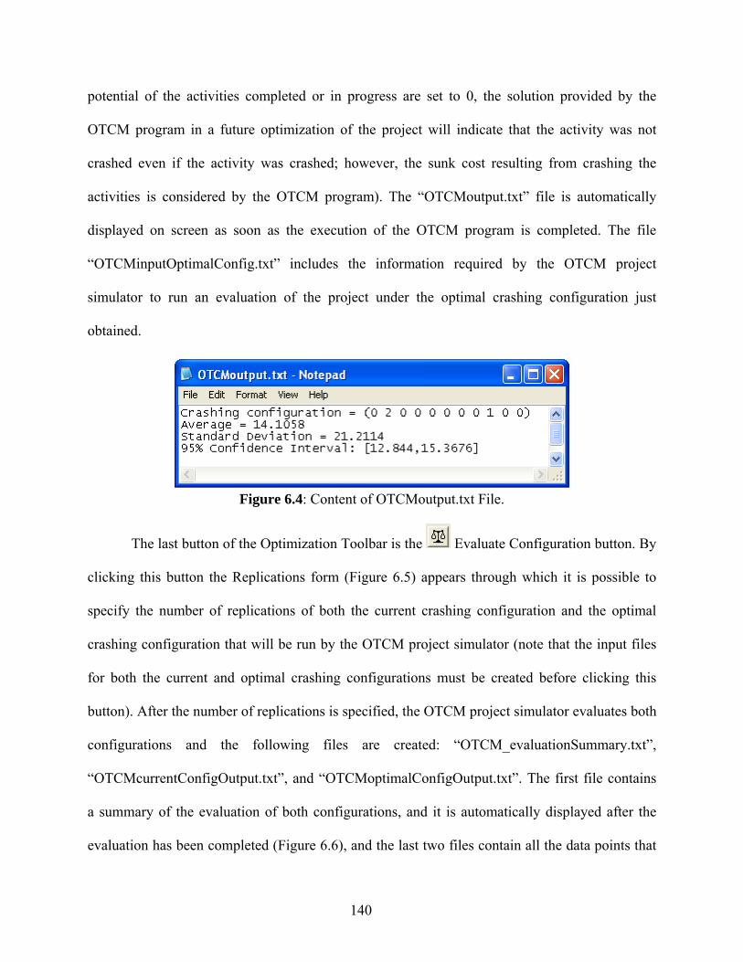
140
potential of the activities completed or in progress are set to 0, the solution provided by the
OTCM program in a future optimization of the project will indicate that the activity was not
crashed even if the activity was crashed; however, the sunk cost resulting from crashing the
activities is considered by the OTCM program). The “OTCMoutput.txt” file is automatically
displayed on screen as soon as the execution of the OTCM program is completed. The file
“OTCMinputOptimalConfig.txt” includes the information required by the OTCM project
simulator to run an evaluation of the project under the optimal crashing configuration just
obtained.
Figure 6.4: Content of OTCMoutput.txt File.
The last button of the Optimization Toolbar is the Evaluate Configuration button. By
clicking this button the Replications form (Figure 6.5) appears through which it is possible to
specify the number of replications of both the current crashing configuration and the optimal
crashing configuration that will be run by the OTCM project simulator (note that the input files
for both the current and optimal crashing configurations must be created before clicking this
button). After the number of replications is specified, the OTCM project simulator evaluates both
configurations and the following files are created: “OTCM_evaluationSummary.txt”,
“OTCMcurrentConfigOutput.txt”, and “OTCMoptimalConfigOutput.txt”. The first file contains
a summary of the evaluation of both configurations, and it is automatically displayed after the
evaluation has been completed (Figure 6.6), and the last two files contain all the data points that

141
were generated to compute the statistics of both the current and the OTCM configuration (these
data points can be used to create the histogram of project completion time and project cost under
both crashing configurations).
Figure 6.5: Form Used to Specify the Number of Replications to be Run for the Evaluation of
the current and OTCM Configuration.
Figure 6.6: Sample File Produced After Evaluating the Current and OTCM Configuration.
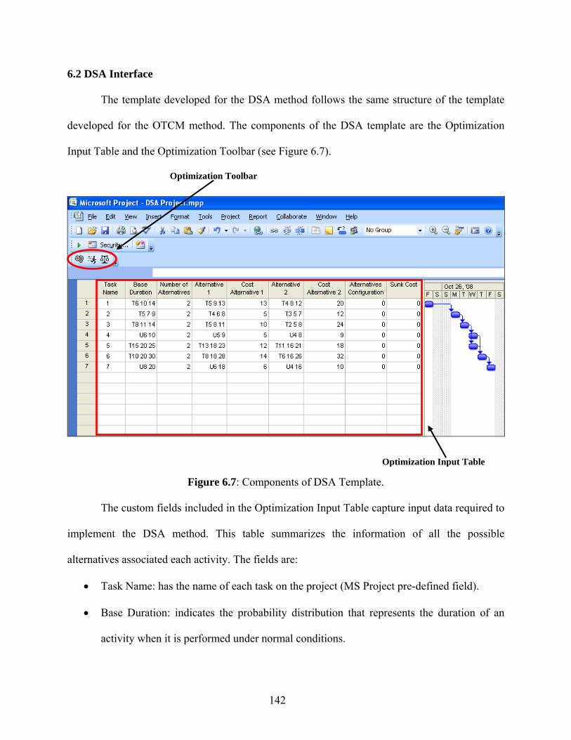
142
6.2 DSA Interface
The template developed for the DSA method follows the same structure of the template
developed for the OTCM method. The components of the DSA template are the Optimization
Input Table and the Optimization Toolbar (see Figure 6.7).
Figure 6.7: Components of DSA Template.
The custom fields included in the Optimization Input Table capture input data required to
implement the DSA method. This table summarizes the information of all the possible
alternatives associated each activity. The fields are:
• Task Name: has the name of each task on the project (MS Project pre-defined field).
• Base Duration: indicates the probability distribution that represents the duration of an
activity when it is performed under normal conditions.
Optimization Toolbar
Optimization Input Table

143
• Number of Alternatives: indicates how many different alternatives are associated with
each activity (in addition to the Base Duration).
• Alternative i: indicates the probability distribution that represents the duration of an
activity when alternative i is implemented. The template is designed to support up to 5
alternatives. However, this limit could be easily expanded.
• Cost Alternative i: indicates the cost associated with implementing alternative i.
• Alternatives Configuration: indicates the alternative chosen for each activity (if the
activity is completed) or the alternative that the project manager wants to evaluate using
the project simulator. If it is equal to 0 the base alternative is chosen.
• Sunk Cost: indicates the cost of the alternative chosen for a particular activity, i.e. the
sunk cost of choosing alternative “1” for activity “3” is 24 (see Figure 6.7).
The information associated with the duration of each activity alternative is entered into
the appropriate Activity i field and must follow one of the following formats:
• Beta distribution: “B min mode max”, e.g. B4 5 6;
• Triangular distribution: “T min mode max”, e.g. T6 7 8;
• Uniform distribution: “U min max”, e.g. U20 40;
• Exponential distribution: “E mean”, e.g. E20; or
• Constant: “C duration”, e.g. C20.
The Optimization Toolbar includes the buttons used to control the execution of the DSA
method. The first button is Generate Input File. When clicked, this button calls the Input
Data form through which the user can specify the desired target completion time, the penalty cost
per unit of lateness, and the parameters required by the Industrial Strength COMPASS (ISC)
(this is the same Input Data form used by the OTCM template; see Figure 6.2). As in the OTCM
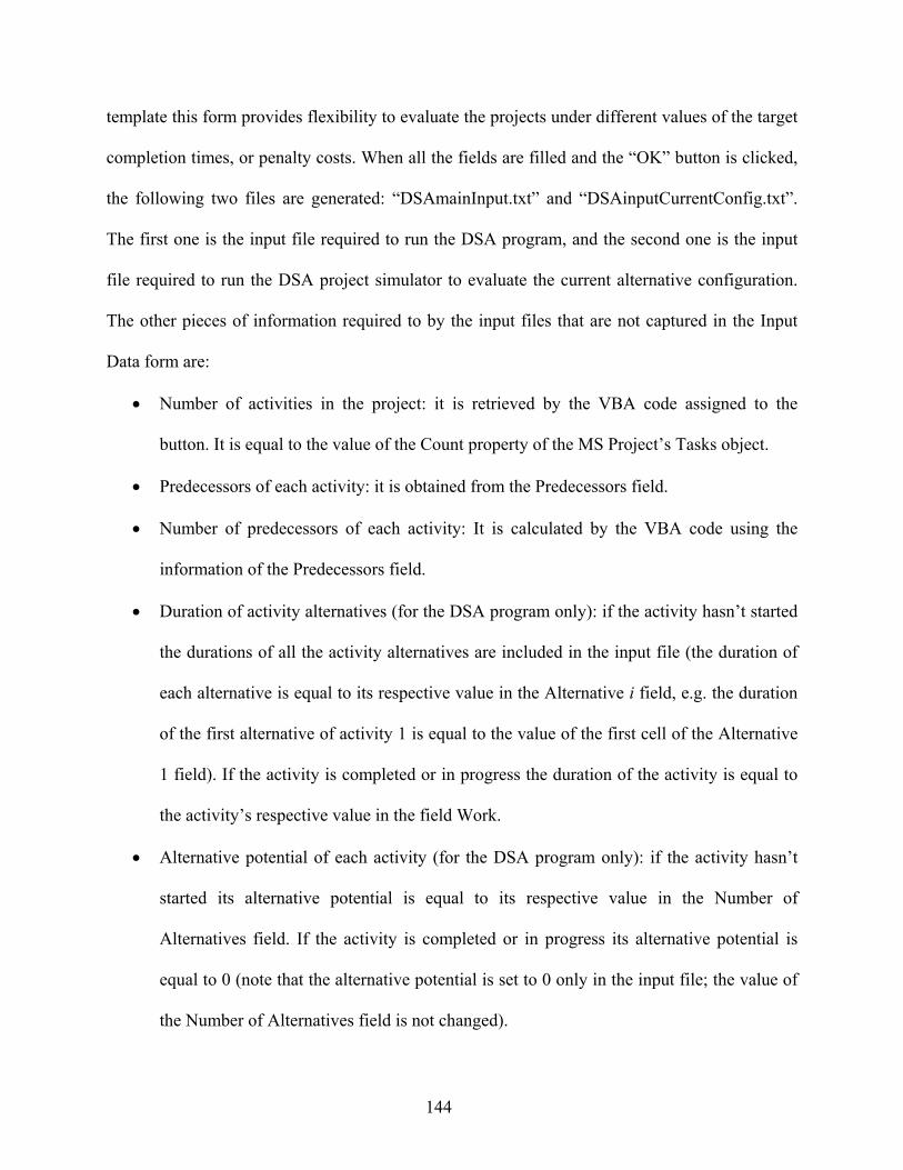
144
template this form provides flexibility to evaluate the projects under different values of the target
completion times, or penalty costs. When all the fields are filled and the “OK” button is clicked,
the following two files are generated: “DSAmainInput.txt” and “DSAinputCurrentConfig.txt”.
The first one is the input file required to run the DSA program, and the second one is the input
file required to run the DSA project simulator to evaluate the current alternative configuration.
The other pieces of information required to by the input files that are not captured in the Input
Data form are:
• Number of activities in the project: it is retrieved by the VBA code assigned to the
button. It is equal to the value of the Count property of the MS Project’s Tasks object.
• Predecessors of each activity: it is obtained from the Predecessors field.
• Number of predecessors of each activity: It is calculated by the VBA code using the
information of the Predecessors field.
• Duration of activity alternatives (for the DSA program only): if the activity hasn’t started
the durations of all the activity alternatives are included in the input file (the duration of
each alternative is equal to its respective value in the Alternative i field, e.g. the duration
of the first alternative of activity 1 is equal to the value of the first cell of the Alternative
1 field). If the activity is completed or in progress the duration of the activity is equal to
the activity’s respective value in the field Work.
• Alternative potential of each activity (for the DSA program only): if the activity hasn’t
started its alternative potential is equal to its respective value in the Number of
Alternatives field. If the activity is completed or in progress its alternative potential is
equal to 0 (note that the alternative potential is set to 0 only in the input file; the value of
the Number of Alternatives field is not changed).

145
• Cost of alternatives of each activity (for the DSA program only): it is obtained from the
Cost Alternative i fields. If an activity is completed or in progress, the cost of the
alternative chosen is set to 0 in the input file (the real cost is represented as sunk cost); for
the activities not started the costs of all activity alternatives are included in the input file
(the cost of each alternative is equal to its respective value in the Cost Alternative i field).
• Cumulative sunk cost: it is equal to the sum of the values of the Sunk Cost field
corresponding to the activities completed or in progress.
• Current configuration of alternatives to be evaluated (for the DSA project simulator
only): for the activities completed or in progress the duration is equal to their respective
value in the field Work, and their cost is set 0 because the cost is represented by the sunk
cost; each one of the remaining activities uses the duration and the cost of the alternative
indicated on the field Alternatives Configuration.
Note that since the alternative potential of activities completed or in progress is set to 0,
the input file will indicate that only the base alternative is available for the activity. Instead of
using the original information associated with the base alternative of the activity in the input file,
the duration of the base alternative included in the input file is represented by the real duration of
the activity, and the cost of the base alternative is set to 0.
As in the OTCM template, in order to determine if an activity is completed, in progress,
or not started the VBA code verifies the value of the field Actual Work of the Work table
corresponding to each activity. If Actual Work is equal to 0 the activity hasn’t started; otherwise,
the activity is completed or in progress.
The second button on the toolbar is Run Optimization. This button calls the DSA
program. Once the DSA program execution is over the following two files are created:

146
“DSAoutput.txt” and “DSAinputOptimalConfig.txt”. The file “DSAoutput.txt” (Figure 6.8)
includes the best configuration of alternatives found by the DSA method as well as the average,
standard deviation, and 95% confidence interval on the project cost resulting from implementing
the solution provided by DSA (note that since the alternative potential of the activities completed
or in progress is set to 0, the solution provided by the DSA program in a future optimization of
the project will indicate that the base alternative of the activity was chosen even when a different
alternative was chosen; however, the sunk cost resulting from the alternative that was actually
chosen is considered by the DSA program). The “DSAouput.txt” file automatically opens and
displays on the screen as soon as the DSA program ends. The file “DSAinputOptimalConfig.txt”
includes the information required by the DSA project simulator to evaluate the project under the
configuration of alternatives just obtained.
Figure 6.8: Content of DSAoutput.txt File.
The last button of the toolbar is the Evaluate Configuration button. By clicking this
button the Replications form (Figure 6.9) appears; through this form it is possible to specify the
number of replications to be run for both the current configuration of alternatives and the
configuration of alternatives provided by the DSA program. After the number of replications is
specified, both configurations are evaluated using the DSA project simulator and the following
files are created: “DSA_evaluationSummary.txt”, “DSAcurrentConfigOutput.txt”, and
“DSAoptimalConfigOutput.txt”. The first file contains a summary of the evaluation of both

147
configurations and it is automatically displayed after the evaluation has been completed (Figure
6.10). The last two files contain all the data points that were generated to compute the statistics
of both the current and the DSA configuration; these data points are also used to plot the
distribution of project cost and project completion time.
Figure 6.9: Form Used to Specify the Number of Replications to be Run for the Evaluation of
the current and DSA Configuration.
Figure 6.10: Sample File Produced After Evaluating the Current and DSA Configuration.

148
6.3 Summary of OTCM and DSA MS Project Templates
The MS Project templates that are developed for the OTCM method and the DSA method
integrate the OTCM and DSA optimization programs and project simulators into MS Project,
allowing project managers to utilize these methods when managing their project. By utilizing the
OTCM or DSA method, project managers may be able to improve the use of their resources and
to reduce the risk of late completion, thus contributing to the improvement of customer
satisfaction, and also improving the profitability of their projects.

149
7. CONCLUSIONS & RECOMMENDATIONS FOR FUTURE RESEARCH
The goal of this research was to address the time-cost tradeoff problem associated with
selecting from among project activity alternatives under uncertainty. Specifically, activities that
make up a project may have several alternatives each with an associated cost and stochastic
distribution of completion time. The result of this effort is the development of two simulation-
based optimization methods: a) Optimal Traditional Crashing Method (OTCM), and b) Dynamic
Selection of Activity Alternatives (DSA) Method. The conclusions drawn for each one of the
methods are presented in the next section.
7.1 Conclusions
The OTCM method addresses a gap identified in the literature, which is the lack of a
stochastic crashing method that provides optimal solutions. The OTCM method was applied to
six different experimental cases to verify its robustness and consistency in finding the optimal
solution (within the tolerance specified by the user). For the simplest case, where there is only
one critical path it was possible to verify that the solution provided by OTCM was the optimal
solution. Since the structure of the information needed by the optimization component of OTCM
is not changed by changing the complexity, the size of the project network, nor the variability of
the activities duration, it is possible to conclude that the OTCM method provided an optimal
solution for each one of the 6 experimental cases to which it was applied. In addition, it was
demonstrated that implementing the dynamic part of the OTCM method provided results that on
average are always equal to or better than the one provided by the static implementation. Out of
the 6 experimental cases, there was only one case where implementing Phase II didn’t improve
upon the results found by Phase I, which was the case of low variability in activity times. That

150
result was expected because the variability in activity time was so small that very little
uncertainty was associated with the duration of each activity, so there was no much room for
improvement when Phase II was applied. Even though Phase II didn’t provide any improvement
in that case with respect to Phase I, it is useful to implement Phase II in all cases because the
variability of certain activities may have been underestimated. If that is the case, it is possible for
those activities to take longer than it was estimated, thus providing an ideal situation for Phase II
to update the optimal solution found in Phase I.
The DSA method expands the current literature related to the time-cost tradeoff problem.
The DSA method is a simulation-based optimization method that relaxes the assumptions
considered by the traditionally defined time-cost tradeoff problems, and provides project
managers with a method that allows a more accurate representation of the situations that may
encounter when managing a project. The DSA method considers that there are different
alternatives associated with each activity, each one having its own distribution of completion
time and associated cost. The method was applied to four experimental cases, and the results
provided were very encouraging. No guarantees can be made about the optimality of the
solutions provided by the method, but the solutions provided by Phase I represented a significant
improvement over using the base alternative of each activity. In addition, the alternatives chosen
for each activity in each one of the experimental cases had a smaller average duration than the
base alternative, which indicates that the method is doing a good job of selecting an appropriate
alternative. Furthermore, in 3 out of the 4 experimental cases, implementing Phase II provided a
significant reduction in cost relative to implementing Phase I; in addition, the results of Phase II
were (on average) always as good or better than the one provided by Phase I. It can be concluded
that DSA Phase II should always be implemented.

151
7.2 Recommendations for Future Research
The OTCM and DSA methods expand the current literature related to the stochastic time-
cost tradeoff problem. The following list provides recommendations for future research that may
further expand the literature related to the stochastic time-cost tradeoff problem:
1) Consider dependent activity times (if the first activities of the project are taking long time
to be completed it is likely that the last activities will also take a long time to be
completed).
2) Consider optimizing alternative cost quantiles (e.g. the 90% percentile rather than the
expected cost).
3) Incorporate flexibility to allow for specifying lead times needed for choosing an
alternative.
4) Investigate alternative reevaluation points.
5) Consider cases where there are at least two projects concurrently managed, and the
available resources should be shared between them.
6) Design a simulation-based optimization engine capable to provide an optimal solution for
the type of problems addressed by the DSA method.

152
REFERENCES
Ahuja, H. N., Dozzi, S. P., & AbouRisk, S. M. (1994). Project Management Techniques in
Planning and Controlling Construction Projects. 2nd Ed., Wiley, New York.
Bissiri, Y., & Dunbar, S. (1999). Resource allocation model for a fast-tracked project.
International Conference on Intelligent Processing and Manufacturing of Materials, 635-
640.
Eisner, H. (2002). Essentials of Project and Systems Engineering Management. 2nd Ed., Wiley,
New York.
Gutjahr, W. J., Strauss, C., &. Wagner, E. (2000). A Stochastic Branch-and-Bound Approach to
Activity Crashing in Project Management. INFORMS journal on computing, 12(2), 125-135.
Haga, W. A. (1998). Crashing PERT networks. Ph.D. Dissertation, University of Northern
Colorado, Colorado.
Haga, W. A., & Marold, K. A. (2004). A simulation approach to the PERT CPM time-cost trade-
off problem. Project Management Journal, 35(2), 31-37.
Haga, W. A., & Marold, K. A. (2005). Monitoring and control of PERT networks. The Business
Review, 3(2), 240-245.
Herroelen, W., & Leus, R. (2005). Project scheduling under uncertainty: Survey and research
potentials. Project Management and Scheduling, 165(2), 289-306.
Hillier, F. S., & Lieberman, G. J. (2001). Introduction to Operations Research. 7th Ed.,
McGraw-Hill, New York.
Hong, L.J. & Nelson, B.L. (2006) Discrete optimization via simulation using COMPASS.
Operations Research, 54(1), 115-129.

153
Kerzner, H. (2003). Project management: a systems approach to planning, scheduling, and
controlling. 8th Ed., Wiley, Hoboken, NJ.
Lee, D. (2005). Probability of project completion using stochastic project scheduling simulation.
Journal of Construction Engineering and Management, 131(3), 310-318.
Lee, D., & Arditi, D. (2006). Automated statistical analysis in stochastic project scheduling
simulation. Journal of Construction Engineering and Management, 132(3), 268-277.
Lu, M., & AbouRizk, S. M. (2000). Simplified CPM/PERT simulation model. Journal of
Construction Engineering and Management, 126(3), 219-226.
MacCrimmon, K. R., & Ryavec, C. A. (1964). An Analytical Study of the PERT Assumptions.
Operations Research, 12(1), 16-37.
Pritsker, A. A. B. (1986). Introduction to Simulation and SLAM II. 3rd Ed., Wiley & Sons, Inc,
New York.
Rosenau, M. D., Githens, G.D., (2005). Successful Project Management : a Step-by-step
Approach with Practical Examples. 4th Ed., Wiley, Hoboken, N.J.
Simmons, L. F. (2002). Project management - critical path method (CPM) and PERT simulated
with Process Model. Proceedings of the 2002 Winter Simulation Conference, Dec 8-11 2002,
1786-1788.
Wiest, J. D., & Levy, F. K. (1969). A management guide to PERT/CPM. Prentice-Hall
Englewood Cliffs, N.J.
Williams, T. (2004). Why Monte Carlo Simulations Of Project Networks Can Mislead. Project
Management Journal, 35(3), 53-61.

154
Xu, J., Nelson, B. L., & Hong, L. J. (2007). Industrial Strength COMPASS: A Comprehensive
Algorithm and Software for Optimization via Simulation.
Website http://users.iems.northwestern.edu/~nelsonb/ISC/.

155
APPENDICES
Appendix A. Industrial Strength COMPASS Input Parameters
The list of ISC parameters that must be included in the input files of the OTCM and DSA
programs is presented in this section (refer to Sections 4.6 and 5.6 for the application of ISC to
the OTCM and DSA methods, and see Figure 4.3 for an example of the ISC parameters). The
ISC parameters are presented in the same order as they should be input (the description of the
ISC input parameters is adapted from Xu et al. (2007) and the document
JieInstructionsMay042008.doc, which was provided by the ISC developers). The ISC parameters
are:
• Text with which the names of the output text files containing ISC sample paths will start;
• Budget of simulation replications;
• Number of ISC macro runs;
• Enable (value of 1) or disable (value of 0) the backtracking test;
• Enable (value of 1) or disable (value of 0) the Optimal Computing Budget Allocation
(OCBA) heuristic;
• Maximum number of generations of the Niching Genetic Algorithm (NGA) without
continuous improvement for transition to local phase to occur;
• Enable (value of 1) or disable (value of 0) the dominant niche transition rule;
• Enable (value of 1) or disable (value of 0) the final clean up procedure;
• Enable (value of 1) or disable (value of 0) the stochastic simulation;
• Value of the indifference zone parameter for the global phase;
• Confidence level parameter for the backtracking test;
• Value of the indifference zone parameter for the backtracking test;

156
• Confidence level parameter for the local optimality test;
• Value of the indifference zone parameter for the local optimality test;
• Confidence level parameter for clean-up;
• Value of the indifference zone parameter for clean-up;
• Initial number of simulation replications assigned to each solution;
• Number of solutions sampled in each local phase iteration;
• Enable (value of 1) or disable (value of 0) the elitism option for the global phase; and
• Constraint pruning frequency.
In order to be executed, ISC requires its own input file. The OTCM program and the
DSA program take the ISC parameters (which are input through the OTCM program or DSA
program input file) and create the input file required by ISC. In addition to these input
parameters, the ISC input file also requires a set of linear constraints that define the range of
possible values for the decision variables considered in the optimization problem. The OTCM
program or the DSA program generate these constraints and write them into the ISC input file
(note that the input files of the OTCM program and DSA program include the maximum
crashing amount (OTCM) or the number of alternatives (DSA), respectively, associated with
every activity, and this information is used to create the linear constraints required by ISC).

157
Appendix B. Input Files for OTCM Experimental Performance Evaluation
The input files used for the OTCM experimental performance evaluation are presented in
this appendix. The OTCM experiments are conducted using an automated version of the OTCM
program, thus it is necessary to specify the number of project instances to be evaluated using
Phase II. The automated version keeps track of the sunk cost; therefore, sunk cost is not input.
10 180 10 600 0 1 1 1 1 1 1 1 1 1 0 1 2 3 4 5 6 7 8 9 3 3 3 3 3 3 3 3 3 3 B10 20 30 B12 14 16 B14 18 22 B12 18 30 B10 20 30 B8 12 16 B18 25 32 B10 20 30 B15 20 25 B6 12 18 9 8 4 6 9 9 1 8 9 4 output 10000000 1 0 -1 -1 0 -1 1 -1 -1 -1 0.01 -1 0.01 0.5 50 10 0 50
Figure B.1: OTCM Experimental Case 1A – Input File.
n T P # Instances NPi Predecessors (PMij = 1 for each j in row i, i = 1,…,n) CPi Activity Duration Distribution (Ai) Crash Costs (CCi) ISC Parameters

158
11 70 40 500 0 1 1 1 1 2 1 1 1 3 1 0 1 1 3 2 2 4 5 6 4 7 8 9 10 3 3 3 3 3 3 3 3 3 3 3 B8 10 12 B6 10 14 B6 8 10 B10 15 20 B12 17 22 B3 5 7 B6 9 12 B4 6 8 B11 13 15 B13 15 17 B5 7 9 6 3 5 4 5 8 5 5 2 8 7 output 100000000 1 0 -1 -1 0 -1 1 -1 -1 -1 0.01 1 0.01 0.5 50 10 0 50
Figure B.2: OTCM Experimental Case 1B – Input File.
n T P # Instances NPi Predecessors (PMij = 1 for each j in row i, i = 1,…,n) CPi Activity Duration Distribution (Ai) Crash Costs (CCi) ISC Parameters

159
13 175 30 500 0 1 1 1 1 1 1 1 1 1 1 1 1 0 1 2 3 4 5 6 7 8 9 10 11 12 3 3 3 3 3 3 3 3 3 3 3 3 3 T9 12 15 T10 13 16 T7 10 13 T11 14 17 T6 9 12 T12 15 18 T11 14 17 T13 16 19 T18 21 24 T5 8 11 T16 19 22 T10 13 16 T12 15 18 11 9 5 7 17 13 8 12 20 17 15 18 5 output 100000000 1 0 -1 -1 0 -1 1 -1 -1 -1 0.01 1 0.01 0.5 50 10 0 50
Figure B.3: OTCM Experimental Case 2A – Input File.
n T P # Instances NPi Predecessors (PMij = 1 for each j in row i, i = 1,…,n) CPi Activity Duration Distribution (Ai) Crash Costs (CCi) ISC Parameters

160
24 50 40 0 0 0 0 1 1 1 1 1 1 1 1 1 1 1 1 1 1 1 1 1 1 1 1 1 0 0 0 1 1 1 1 1 4 5 6 7 8 2 3 3 3 3 3 15 16 17 18 19 5 5 5 5 5 5 5 5 5 5 5 5 5 5 5 5 5 5 5 5 5 5 5 5 B10 20 30 B20 30 40 B10 20 30 B10 15 20 B10 15 20 B10 15 20 B10 15 20 B10 15 20 B10 15 20 B10 15 20 B10 15 20 B10 15 20 B10 15 20 B17 22 27 B10 15 20 B10 15 20 B10 15 20
Figure B.4: OTCM Experimental Case 2B – Input File.
n T P # Instances NPi Predecessors (PMij = 1 for each j in row i, i = 1,…,n) CPi Activity Duration Distribution (Ai)
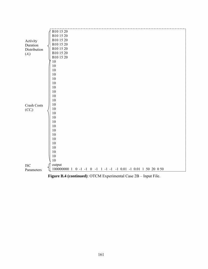
161
B10 15 20 B10 15 20 B10 15 20 B10 15 20 B10 15 20 B10 15 20 B10 15 20 10 10 10 10 10 10 10 10 10 10 10 10 10 10 10 10 10 10 10 10 10 10 10 10 output 100000000 1 0 -1 -1 0 -1 1 -1 -1 -1 0.01 -1 0.01 1 50 20 0 50
Figure B.4 (continued): OTCM Experimental Case 2B – Input File.
Activity Duration Distribution (Ai) Crash Costs (CCi) ISC Parameters

162
13 175 30 500 0 1 1 1 1 1 1 1 1 1 1 1 1 0 1 2 3 4 5 6 7 8 9 10 11 12 3 3 3 3 3 3 3 3 3 3 3 3 3 T11.5 12 12.5 T12.5 13 13.5 T9.5 10 10.5 T13.5 14 14.5 T8.5 9 9.5 T14.5 15 15.5 T13.5 14 14.5 T15.5 16 16.5 T20.5 21 21.5 T7.5 8 8.5 T18.5 19 19.5 T12.5 13 13.5 T14.5 15 15.5 13 15 17 7 18 12 6 8 15 6 14 10 12 output 100000000 1 0 -1 -1 0 -1 1 -1 -1 -1 0.01 0.5 0.01 0.5 50 10 0 4
Figure B.5: OTCM Experimental Case 3A – Input File.
n T P # Instances NPi Predecessors (PMij = 1 for each j in row i, i = 1,…,n) CPi Activity Duration Distribution (Ai) Crash Costs (CCi) ISC Parameters

163
13 185 30 100 0 1 1 1 1 1 1 1 1 1 1 1 1 0 1 2 3 4 5 6 7 8 9 10 11 12 3 3 3 3 3 3 3 3 3 3 3 3 3 T6 12 18 T7 13 19 T4 10 16 T8 14 20 T13 19 25 T9 15 21 T8 14 20 T10 16 22 T15 21 27 T12 18 24 T13 19 25 T7 13 19 T9 15 21 15 12 15 9 8 11 7 6 11 8 6 12 14 output 100000000 1 0 -1 -1 0 -1 1 -1 -1 -1 0.01 1 0.01 0.5 50 10 0 50
Figure B.6: OTCM Experimental Case 3B – Input File.
n T P # Instances NPi Predecessors (PMij = 1 for each j in row i, i = 1,…,n) CPi Activity Duration Distribution (Ai) Crash Costs (CCi) ISC Parameters

164
Appendix C. Input Files for DSA Experimental Performance Evaluation
The input files used for the DSA experimental performance evaluation are presented in
this appendix. The DSA experiments are performed using an automated version of the DSA
program, thus it is necessary to specify the number of project instances to be evaluated using
Phase II. The automated version keeps track of the sunk cost; therefore, sunk cost is not input.
7 80 35 700 0 1 1 1 1 2 1 0 1 2 3 3 4 5 6 2 2 2 2 2 2 2 T6 10 14 T5 9 13 T4 8 12 T5 7 9 T4 6 8 T3 5 7 T8 11 14 T5 8 11 T2 5 8 U6 10 U5 9 U4 8 T15 20 25 T13 18 23 T11 16 21 T10 20 30 T8 18 28 T6 16 26 U8 20 U6 18 U4 16 0 13 20 0 5 12 0 10 24 0 5 9 0 12 18 0 14 32 0 6 10 output 10000000 1 0 -1 -1 0 -1 1 -1 -1 -1 0.01 -1 0.01 0.5 50 10 0 50
Figure C.1: DSA Experimental Case 1A – Input File.
n T P # Instances NPi Predecessors (PMij = 1 for each j in row i, i = 1,…,n) APi Distribution Of Duration Of Activity Alternatives (Aij) Cost of Alternative (CAij) ISC Parameters

165
15 120 10 1000 0 1 1 2 1 1 1 2 2 2 2 1 1 2 1 0 1 1 2 3 4 4 4 5 6 6 7 8 9 8 9 10 11 12 13 14 0 0 2 2 0 2 0 0 2 2 0 0 2 2 0 B10 15 20 T5 7 9 B15 20 25 B13 18 23 B11 16 21 T13 16 19 T12 15 18 T11 14 17 T6 10 14 B10 20 30 B7 17 27 B5 15 25 T8 14 20 B4 6 8 T6 7 8 T5 6 7 T3 4 5 B14 16 18 B12 14 16 B11 13 15 T12 16 20 T10 15 20 B14 15 16 B13 14 15 B12 13 14 T10 16 22 T8 14 20 T6 12 18 B4 7 10 0 0 0 4 10 0 3 9 0 0 5 10 0 0 0 9 20 0 6 10 0 0
Figure C.2: DSA Experimental Case 1B – Input File.
n T P # Instances NPi Predecessors (PMij = 1 for each j in row i, i = 1,…,n) APi Distribution Of Duration Of Activity Alternatives (Aij) Cost of Alternative (CAij)
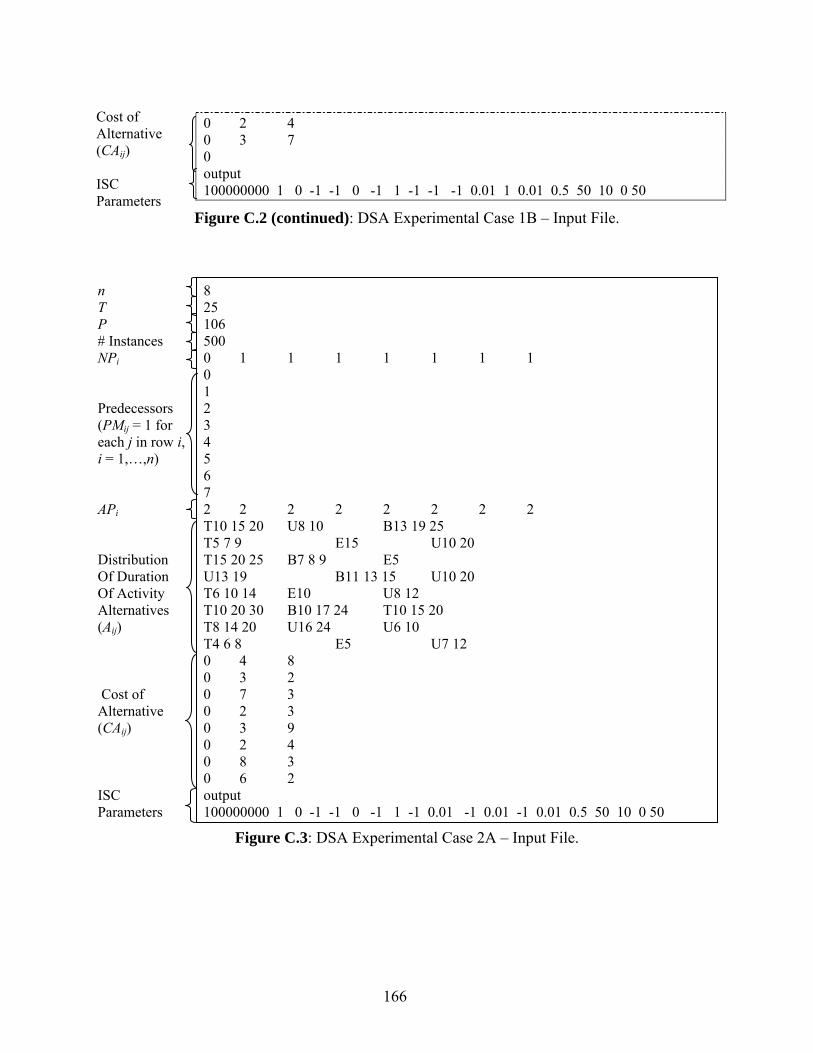
166
0 2 4 0 3 7 0 output 100000000 1 0 -1 -1 0 -1 1 -1 -1 -1 0.01 1 0.01 0.5 50 10 0 50
Figure C.2 (continued): DSA Experimental Case 1B – Input File.
8 25 106 500 0 1 1 1 1 1 1 1 0 1 2 3 4 5 6 7 2 2 2 2 2 2 2 2 T10 15 20 U8 10 B13 19 25 T5 7 9 E15 U10 20 T15 20 25 B7 8 9 E5 U13 19 B11 13 15 U10 20 T6 10 14 E10 U8 12 T10 20 30 B10 17 24 T10 15 20 T8 14 20 U16 24 U6 10 T4 6 8 E5 U7 12 0 4 8 0 3 2 0 7 3 0 2 3 0 3 9 0 2 4 0 8 3 0 6 2 output 100000000 1 0 -1 -1 0 -1 1 -1 0.01 -1 0.01 -1 0.01 0.5 50 10 0 50
Figure C.3: DSA Experimental Case 2A – Input File.
Cost of Alternative (CAij) ISC Parameters
n T P # Instances NPi Predecessors (PMij = 1 for each j in row i, i = 1,…,n) APi Distribution Of Duration Of Activity Alternatives (Aij) Cost of Alternative (CAij) ISC Parameters

167
16 92 50 500 0 1 1 1 2 1 2 2 1 1 1 2 1 2 2 2 0 1 1 2 2 3 3 4 5 5 6 7 8 9 9 10 10 11 12 12 13 14 15 0 0 2 2 0 2 0 0 2 2 2 0 0 2 0 0 U5 10 T8 10 12 T10 15 25 U12 15 T15 30 35 E6 T12 15 18 U8 22 T15 20 25 U12 18 E15 U5 12 T6 12 14 T4 6 10 E21 U7 20 T6 12 18 T5 6 7 T3 6 9 E10 U10 20 T7 12 17 U12 16 U15 20 T7 9 11 U4 6 U4 8 T12 14 20 T4 7 10 T10 15 20
Figure C.4: DSA Experimental Case 2B – Input File.
n T P # Instances NPi Predecessors (PMij = 1 for each j in row i, i = 1,…,n) APi Distribution Of Duration Of Activity Alternatives (Aij)

168
0 0 0 17 22 0 11 7 0 0 16 4 0 0 0 12 11 0 21 10 0 12 30 0 0 0 5 22 0 0 output 100000000 1 0 -1 -1 0 -1 1 -1 -1 -1 0.1 -1 0.1 1 50 10 0 50
Figure C.4 (continued): DSA Experimental Case 2B – Input File.
Cost of Alternative (CAij) ISC Parameters

169
Appendix D. OTCM/DSA MS Project Template – User Manual
This appendix presents a step-by-step example that illustrates how to use the DSA
template to apply the DSA method to a project (note that the steps that are shown in this example
also apply for the OTCM MS Project template). To illustrate the procedure, the DSA Sample
Project presented in Chapter 5 is considered. Table D.1 describes the project and Figure D.1
depicts graphically the project network. The target completion time of the project is 65 and the
lateness penalty is defined as
⎩⎨⎧
>−≤
=65τif),65τ(10065τif,0
)τ,(TPF.
Table D.2 shows the duration of each activity alternative for the project instance that is
considered.
Table D.1: DSA Sample Project Specifications. Alternative Cost
Activity Base 1 2 1 2 Predecessors1 T10 15 20 - - - - - 2 T10 20 30 U15 30 U10 20 10 30 1 3 T15 20 25 T7 8 9 E13 25 15 2 4 U13 19 T11 13 15 U10 28 10 10 3
1 2 3 4
Figure D.1: DSA Sample Project Network.
Table D.2: DSA Sample Project Instance.
Alternative Cost Activity Base 1 2 1 2
1 17.48 - - 2 21.23 18.68 11.08 10 30 3 22.21 8.02 3.64 25 15 4 16.52 12.23 12.01 10 10

170
The first step in the process is to create a MS Project file for the project using the DSA
template. Open the DSA template and then click the Save button located in the Standard toolbar
to create the file. Once the file is created it is necessary to input the information that defines the
structure of the project network; this information is input through the Entry table (Figure D.2),
which is display as soon as the DSA template is open. The fields that must be completed in the
Entry table in order to apply the DSA method are Task Name and Predecessors (note that there
are many other fields that the project managers might fill when defining their projects, but only
the two mentioned above are considered by the DSA method).
Figure D.2: Entry View.
After populating the fields of the Entry table it is time to input the information that
defines the optimization problem. This information is input through the Optimization Input table.
To access this table, go to the View menu and click on the Optimization Input table (see Figure
D.3); any table can be accessed through the View menu in a similar way. In the Optimization
Input table (Figure D.4) it is necessary to input the base duration of the activity, the number of
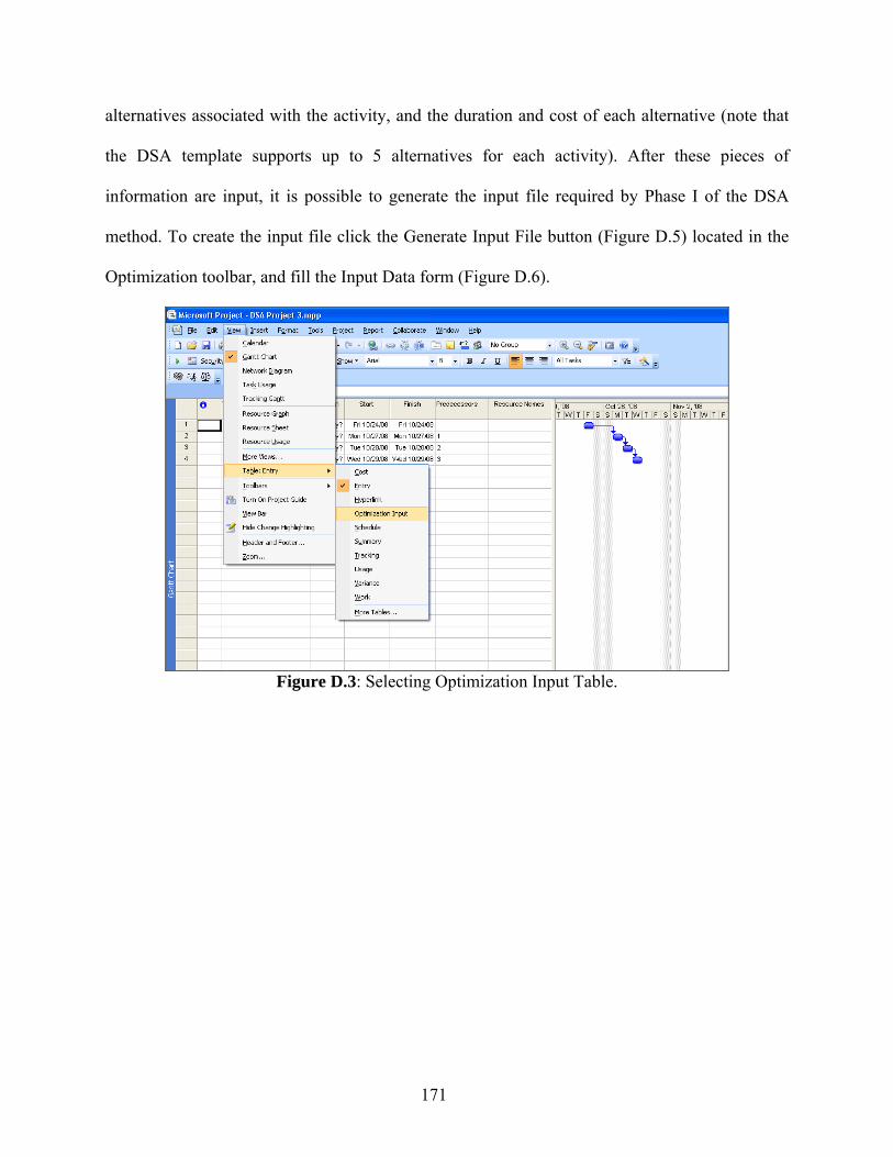
171
alternatives associated with the activity, and the duration and cost of each alternative (note that
the DSA template supports up to 5 alternatives for each activity). After these pieces of
information are input, it is possible to generate the input file required by Phase I of the DSA
method. To create the input file click the Generate Input File button (Figure D.5) located in the
Optimization toolbar, and fill the Input Data form (Figure D.6).
Figure D.3: Selecting Optimization Input Table.

172
Figure D.4: Optimization Input Table.
Figure D.5: Location of the Generate Input File Button.
Generate Input File Button

173
Figure D.6: Input Data Form.
The Input Data form is used to input the target completion time, the penalty cost per unit
of lateness, and the parameters required by ISC (refer to Chapter 6.2 for additional details about
the Input Data form). The input file required by the DSA program is generated (and saved in the
folder where the MS Project file generated using the DSA template is saved) by clicking the OK
button of the Input Data form. The input file required by the DSA project simulator to evaluate
the current configuration of alternatives, which at this point (before the start of the project) is to
choose the base alternative for each activity, is also generated. Once the input file required by the
DSA program is created, the Run Optimization button is clicked (Figure D.7) to execute the
DSA program. Once the DSA program has run to completion, the solution identified is written to
the DSAoutput.txt file, and it is automatically displayed (Figure D.8); the input file required by

174
the DSA project simulator to evaluate the optimal crashing configuration is another output of the
DSA program.
Figure D.7: Location of the Run Optimization Button.
Figure D.8: Solution Identified by the DSA Program.
Run Optimization Button

175
The solution identified by the DSA program indicates that activities 3 and 4 should be
completed with their alternative #1, resulting in an average project cost of 38.30. To compare the
impact that this configuration and the current configuration of alternatives have on the average
project cost and the average project completion time, the DSA project simulator is executed. The
Evaluate Configuration button (Figure D.9) is clicked to display the Replications form (Figure
D.10), which is used to specify the number of project instances that will be simulated under each
configuration (in this example 50,000 project instances are evaluated under each configuration).
Figure D.9: Location of the Evaluate Configuration Button.
By clicking the OK button of the Replications form the DSA project simulator is
executed. The DSA project simulator generates three output files: DSA_evaluationSummary.txt,
DSAcurrentConfigOutput.txt, and DSAoptimalConfigOutput.txt. The first file, which is
automatically displayed, includes statistics about project cost and project completion time for the
two configurations that are evaluated (Figure D.11). The last two files include the data points
that are used to compute the time and cost statistics for the current configuration of alternatives
Evaluate Configuration Button

176
and the configuration of alternatives identified by the DSA program, respectively. These data
points can also be used to generate empirical distributions of project cost and project completion
time.
Figure D.10: Replications Form.

177
Figure D.11: DSA_evaluationSummary.txt File.
The results that are presented in the DSA_evaluationSummary.txt file indicate that the
average cost of the project when the solution identified by the DSA program is implemented is
significantly smaller than the average cost when the current configuration of alternatives is
implemented.
Assuming that the project manager proceeds with the configuration of alternatives
provided by prior to the start of the project, activity 1 is completed using its base alternative and
its resulting duration is 17.48 (see Table D.2). In order to update the project status, this
information is included in the Work and Actual Work fields of MS Project (note that the project
manager may have specified a value in the Work field before the project start, but this value is
updated when the activity is completed to reflect the real work). The Work and Actual Work

178
fields are located in the Work table. Figure D.12 shows the Work table with the fields Work and
Actual Work indicating the work (which is used as the actual activity duration for activities
completed or in progress in the DSA program and DSA project simulator) of activity 1.
Figure D.12: Work Table.
After completing activity 1, the project proceeds and activity 2 is completed. The
duration of activity 2 is 21.23, and it is included in the Work and Actual fields. At this time the
first reevaluation point, which is the start time of activity 3, is encountered. Note that if there
were an activity in progress by the time a reevaluation point is reached, the project manager must
update the Work and Actual Work fields to indicate the status of the activity. In this case the
value input in the Work field is considered as an accurate estimate of the total work required by
the activity, and the value input in the Actual Work field indicates the amount of work performed
up to that time. In addition, any information about the activity alternatives can be updated before
the reevaluation, such as the inclusion of a new alternative for an activity or a new cost for an
activity alternative previously defined.
Before running the DSA program again, the Generate Input File button is clicked to
generate updated input files for the DSA program and the DSA project simulator, which reflect

179
the current status of the project. After the new input file is generated the Run Optimization
button is clicked and the new configuration of alternatives is displayed (Figure D.13).
Figure D.13: Solution Identified at First Reevaluation.
The new solution indicates that alternative #1 is to be chosen for activity 3 (as indicated
by the solution identified prior to the start of the project), and that activity 4 is to be completed
with the current resources (base alternative). The resulting average project of this configuration
is 30.54.
Before proceeding with the project the project manager might be interested in evaluating
the impact that a configuration different that the one identified by the DSA program has on the
average project cost. Let’s assume that the project manager wants to evaluate the impact of
choosing alternative #2 for activities 3 and 4. To do that, the project manager specify the
configuration to be evaluated in the Alternatives Configuration field and click the Generate Input

180
File button to generate an updated input file for the DSA project simulator, which indicates the
configuration to be evaluated (recall that an input file is also generated for the DSA program
when the Generate Input File button is clicked, but in this case the new input file is equal to the
one created before the first reevaluation because the status of the project network is the same).
After creating the input file, the new configuration is compared to the one just found by the DSA
program by clicking the Evaluate Configuration button. The comparison for 50,000 simulated
instances of the project under each configuration is shown in Figure D.14.
Figure D.14: Comparison of Configurations.
The average project cost when the configuration specified by the project manager is used
is extremely high (830.32). Therefore, the project proceeds using alternative #1 for activity 3 as
indicated by the configuration identified by the DSA program; the resulting duration of the

181
activity is 8.02. The Work and Actual Work tables are updated with the duration of activity 3.
The field Alternatives Configuration, located at the Optimization Input table, is also updated to
indicate the alternative chosen for activity 3 (Figure D.15). The Sunk Cost field is automatically
updated and shows the cost of alternative #1.
Figure D.15: Updated Optimization Input Table.
If the project manager follows the DSA method as explained in Chapter 5, the project
would proceed using the base alternative for activity 4. The project manager could also decide to
run another reevaluation of the project network before starting activity 4 just to confirm that it is
not necessary to use an alternative for activity 4. To run an additional reevaluation, an updated
input file is generated (by clicking the Generate Input File button), and the DSA program is
executed again. The result of that evaluation is shown in Figure D.16. The new solution confirms
that activity 4 is to be completed using the base alternative. Note that the new solution indicates a
0 (base alternative) for activity 3; this is because activity 3 is completed by the time of the
reevaluation and its alternative potential is set to 0 in the input file before running the DSA
program (recall Chapter 6.2). This means that the DSA program only determines which
alternative to choose for the activities that haven’t started by the time of the reevaluation.

182
Figure D.16: Solution Identified at Additional Reevaluation.

183
Appendix E. CD Contents
The enclosed CD contains the MS Project Template developed for OTCM and DSA. In
addition, the CD contains the C++ code files used to generate the OTCM Project Simulator,
OTCM Program, DSA Project Simulator, and DSA Program (note that all these programs were
compiled using Visual C++, but they can be compiled using other C++ compilers). A description
for each one of the folders included in the CD is provided below:
• OTCM Template: This folder contains all the files necessary to use the OTCM Template.
Copy this folder to your computer and double click the “OTCM Template” MS Project
template file to use the template. In addition, this folder contains the MS Project file
created with the OTCM template for the example presented in Chapter 4.
• OTCM Program C++ Code: This folder contains all the C++ files required to compile the
OTCM Program. This folder has three sub-folders, which include: 1) C++ files of the
project simulator used by the OTCM program, 2) ISC C++ files and lp_solve C++ files
(lp_solve is an open-source linear programming solver library used by ISC), and 3) ISC
C++ files that are modified to facilitate the interaction between the project simulator and
ISC, respectively. In addition, the second subfolder includes the
“JieinstructionsMay042008” file, which provides instructions for compiling ISC in
Visual C++ (the OTCM Program is compiled following the same steps).

184
• OTCM Project Simulator C++ Code: This folder contains all the C++ files required to
compile the OTCM project simulator that is used to compare different crashing
configurations.
• DSA Template: This folder contains all the files necessary to use the DSA Template.
Copy this folder to your computer and double click the “DSA Template” MS Project
template file to use the template. In addition, this folder contains the MS Project file
created with the DSA template for the example presented in Chapter 5 and in
Appendix D.
• DSA Program C++ Code: This folder contains all the C++ files required to compile the
DSA Program. This folder has three sub-folders, which include: 1) C++ files of the
project simulator used by the DSA program, 2) ISC C++ files and lp_solve C++ files, and
3) ISC C++ files that are modified to facilitate the interaction between the DSA project
simulator and ISC, respectively. In addition, the second subfolder includes the
“JieinstructionsMay042008” file, which provides instructions for compiling ISC in
Visual C++ (the DSA Program is compiled following the same steps).
• DSA Project Simulator C++ Code: This folder contains all the C++ files required to
compile the version of the DSA project simulator that is used to compare different
configurations of alternatives.