1

Project number: 265138 Project name: New methodologies for multi-hazard and multi-risk

assessment methods for Europe Project acronym: MATRIX Theme: ENV.2010.6.1.3.4

Multi-risk evaluation and mitigation strategies Start date: 01.10.2010 End date: 30.09.2013 (36 months) Deliverable: D7.1 Report on the MATRIX common IT platform Version: v2 Responsible partner: ETHZ Month due: M12 Month delivered: M20 Primary author: Dr. Arnaud Mignan (ETHZ) 30.01.2012 _______________________________ _________________ Signature Date Reviewer: Pranab Kini (UBC) 10.02.2012 _______________________________ _________________ Signature Date Authorised: Jochen Zschau (GFZ) 31.05.2012

_______________________________ _________________ Signature Date

Dissemination Level

PU Public

PP Restricted to other programme participants (including the Commission Services)

RE Restricted to a group specified by the consortium (including the Commission Services)

CO Confidential, only for members of the consortium (including the Commission Services)

x

2

Abstract Test cases provide an opportunity to apply multi-hazard and multi-risk methodologies to real world conditions. This allows the study of the potential and limitations of the innovative approaches being developed within the context of the MATRIX project. Such studies are of critical importance for formulating recommendations to decision makers. Such a mission within the MATRIX project will be undertaken by the conception and development of a MATRIX common IT platform, which will include a critical component referred to within the project as the Virtual City, which integrates the setup of test cases, multi-hazard and multi-risk analysis and sensitivity tests. The proposed platform will implement the hazards and their various interdependencies, which can be anticipated in Europe. Although the focus will be on the three MATRIX test sites: Naples (Italy), French West Indies and Cologne (Germany), other multi-type hazard and risk scenarios, while not realistic for these test sites but plausible elsewhere, can be implemented via the concept of Virtual City. This report presents the different steps of the conception and development of the MATRIX multi-risk platform. First, it gives an overview of the modular structure and IT architecture of the proposed software. Then, a first build (“platform sketch”) is described in which multi-type hazard and risk modelling strategies are evaluated. Next follows a review of single-risk and multiple single-risk tools for assessing the availability and usability of standard methodologies (e.g., single hazard computation) and IT frameworks. Finally, guidelines are provided to implement the multi-type hazard and risk framework into a sophisticated IT platform (second build), the so-called MATRIX platform.

Keywords: multi-risk platform, IT system architecture, test sites, virtual city

3

Acknowledgments

The research leading to these results has received funding from the European Community’s Seventh Framework Programme [FP7/2007-2013] under grant agreement n° 265138.

4

Table of contents Abstract 2 Acknowledgments 3 Table of contents 4 List of Figures 7 List of Tables 8 1 Generalities 9 1.1 NEED FOR A MULTI-RISK PLATFORM 9 1.2 BUILDING A MULTI-RISK PLATFORM 9 1.2.1 Platform Modular Structure Overview 10 1.2.2 IT System Architecture Overview 11 1.2.3 Virtual City and Test Sites 12 2 Build v. 0.x (“Platform Sketch”): Multi-Risk Modelling Procedures Assessment

14

2.1 BASICS OF STANDARD SINGLE-RISK MODELLING 14 2.1.1 Pre-computed Stochastic Event Sets 14 2.1.2 Damage Engine 14 2.1.3 Risk Metrics Engine 15 2.2 SEQUENTIAL MONTE CARLO SIMULATION 16 2.3 SAMPLING PROCEDURES 17 2.3.1 Definition of Event Time Series 17 2.3.2 A Note on Bayesian Event Trees and Propagation of Uncertainties 24 2.4 TIME-DEPENDENT RATE ENGINE CONCEPTUALIZATION 27 2.4.1 Implementation of Renewal Processes 29 2.4.2 Implementation of Event Interaction 30 2.4.3 Time-Dependent Rate Engine Blueprint 34 2.5 TIME-DEPENDENT VULNERABILITY ENGINE CONCEPTUALIZATION 36 2.5.1 Time-Dependent Vulnerability Engine Blueprint 37 2.5.2 Implementation of Functional Vulnerability as a Platform Add-On 40 2.6 HEURISTIC DATABASES – VIRTUAL CITY BASICS 40 2.6.1 Data Simulation for a Generic Time-Dependent Earthquake Scenario 41 2.6.2 Real Data Implementation for a Generic Time-Dependent Earthquake Scenario

47

2.7 LESSONS LEARNED & GUIDELINES TO BUILD v. 1.x 49 3 Review of Hazard and Risk Modelling Tools 50 3.1 RISK PLATFORMS 50 3.1.1 HAZUS 50 3.1.2 OpenGEM 50

5

3.1.3 CAPRA-GIS 51 3.1.4 Armagedom 52 3.1.5 ByMuR Project 52 3.1.6 RiskScape 53 3.2 HAZARD MODELS 54 3.2.1 Seismic 55 3.2.2 Volcanic 56 3.2.3 Flood (Fluvial & Coastal) 56 3.2.4 Meteorological (Winter Storm, Cold & Heat Wave) 57 3.2.5 Tsunami 57 3.2.6 Landslide 57 3.2.7 Wildfire 58 3.2.8 Fire Following an Event 58 3.2.8 Industrial 58 3.3 SOCIO-ECONOMIC IMPACT 59 3.3.1 Disaster Response Network Enabled Platform 59 3.3.2 CATastrophe SIMulator 60 3.3.3 Social and Economic Impact Module (OpenGEM) 61 3.4 VISUALISATION 61 3.4.1 SHARE Visualization Interface 61 3.4.2 OneGeology 62 3.4.3 Lessons Learned from the ARMONIA Project 62 3.5 DATA MODELS 63 3.5.1 NRML (OpenGEM) 63 3.5.2 GeoSciML 64 3.5.3 RiskScape 64 4 Build v. 1.x (MATRIX Common IT Platform): IT Architecture Development

66

4.1 PREREQUISITES 66 4.1.1 Resources 66 4.1.2 Other Prerequisites 66 4.2 ASPECTS OF SOFTWARE ENGINEERING 66 4.2.1 Development Approach 66 4.2.2 Development Systems 67 4.2.3 Programming and Data Exchange Languages 68 4.2.4 Data Model 68 4.2.5 Data Stores 69 4.2.6 User Interface 69 4.2.7 Testing 70 4.2.8 License 70 4.3 DATA STRUCTURES 70 5 Conclusions 72

6

Glossary 73 References 76

7

List of Figures Fig. 1 Modular structure of the MATRIX multi-risk platform 10 Fig. 2 Three-tiered architecture of the MATRIX multi-risk platform 12 Fig. 3 Poisson and Negative Binomial distributions 19 Fig. 4 Event time series from different distributions 23 Fig. 5 Logic tree approach to risk modelling 24 Fig. 6 Example of different Beta distributions 26 Fig. 7 From a Bayesian event tree to an event table 27 Fig. 8 Flow chart linking the TD rate engine to the sequential simulation 28 Fig. 9 Lognormal renewal process 30 Fig. 10 Intra- and inter-hazard interaction 31 Fig. 11 Static stress transfer 34 Fig. 12 TD rate engine blueprint 35 Fig. 13 Flow chart linking the TD vulnerability engine to the sequential

simulation 37

Fig. 14 TD (physical) vulnerability and damage engines blueprint 39 Fig. 15 Proposed bridge between MATRIX and socio-economic platforms 40 Fig. 16 3-fault system for the Virtual City scenario 44 Fig. 17 Exposure spatial distribution for the Virtual City scenario 45 Fig. 18 Exceedance probability curves for the Virtual City scenario 46 Fig. 19 Difference in aggregate losses for different return periods 47 Fig. 20 ShakeMap PGA footprints of historical cascade events 48 Fig. 21 Examples of flood hazard footprints 57 Fig. 22 Example of landslide hazard footprint 58 Fig. 23 CATSIM framework 60 Fig. 24 Example screenshot of the SHARE portal page 62 Fig. 25 Colour scale proposed by ARMONIA project for mapping risk 63 Fig. 26 Example screenshot of the web-based Jenkins user interface 67 Fig. 27 UML class diagram of the data model for MATRIX 69

8

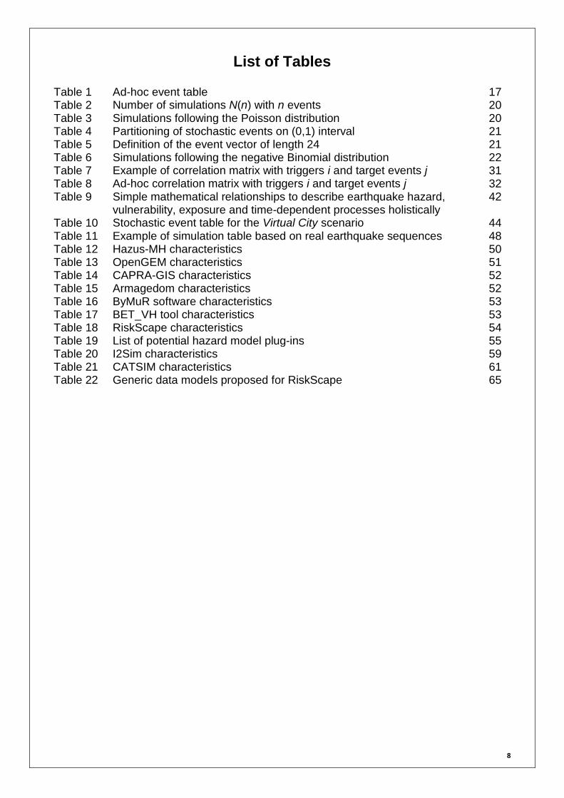
List of Tables Table 1 Ad-hoc event table 17 Table 2 Number of simulations N(n) with n events 20 Table 3 Simulations following the Poisson distribution 20 Table 4 Partitioning of stochastic events on (0,1) interval 21 Table 5 Definition of the event vector of length 24 21 Table 6 Simulations following the negative Binomial distribution 22 Table 7 Example of correlation matrix with triggers i and target events j 31 Table 8 Ad-hoc correlation matrix with triggers i and target events j 32 Table 9 Simple mathematical relationships to describe earthquake hazard,

vulnerability, exposure and time-dependent processes holistically 42

Table 10 Stochastic event table for the Virtual City scenario 44 Table 11 Example of simulation table based on real earthquake sequences 48 Table 12 Hazus-MH characteristics 50 Table 13 OpenGEM characteristics 51 Table 14 CAPRA-GIS characteristics 52 Table 15 Armagedom characteristics 52 Table 16 ByMuR software characteristics 53 Table 17 BET_VH tool characteristics 53 Table 18 RiskScape characteristics 54 Table 19 List of potential hazard model plug-ins 55 Table 20 I2Sim characteristics 59 Table 21 CATSIM characteristics 61 Table 22 Generic data models proposed for RiskScape 65

9

1 Generalities 1.1 NEED FOR A MULTI-RISK PLATFORM

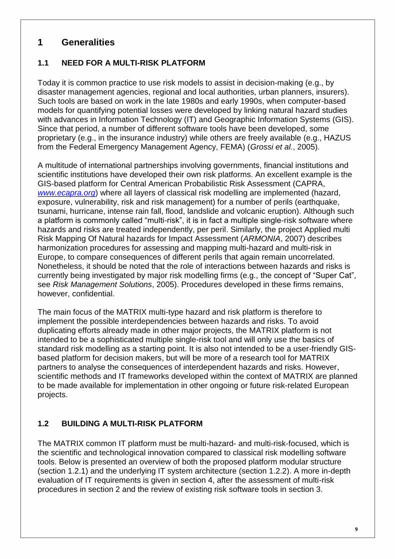
Today it is common practice to use risk models to assist in decision-making (e.g., by disaster management agencies, regional and local authorities, urban planners, insurers). Such tools are based on work in the late 1980s and early 1990s, when computer-based models for quantifying potential losses were developed by linking natural hazard studies with advances in Information Technology (IT) and Geographic Information Systems (GIS). Since that period, a number of different software tools have been developed, some proprietary (e.g., in the insurance industry) while others are freely available (e.g., HAZUS from the Federal Emergency Management Agency, FEMA) (Grossi et al., 2005). A multitude of international partnerships involving governments, financial institutions and scientific institutions have developed their own risk platforms. An excellent example is the GIS-based platform for Central American Probabilistic Risk Assessment (CAPRA, www.ecapra.org) where all layers of classical risk modelling are implemented (hazard, exposure, vulnerability, risk and risk management) for a number of perils (earthquake, tsunami, hurricane, intense rain fall, flood, landslide and volcanic eruption). Although such a platform is commonly called “multi-risk”, it is in fact a multiple single-risk software where hazards and risks are treated independently, per peril. Similarly, the project Applied multi Risk Mapping Of Natural hazards for Impact Assessment (ARMONIA, 2007) describes harmonization procedures for assessing and mapping multi-hazard and multi-risk in Europe, to compare consequences of different perils that again remain uncorrelated. Nonetheless, it should be noted that the role of interactions between hazards and risks is currently being investigated by major risk modelling firms (e.g., the concept of “Super Cat”, see Risk Management Solutions, 2005). Procedures developed in these firms remains, however, confidential. The main focus of the MATRIX multi-type hazard and risk platform is therefore to implement the possible interdependencies between hazards and risks. To avoid duplicating efforts already made in other major projects, the MATRIX platform is not intended to be a sophisticated multiple single-risk tool and will only use the basics of standard risk modelling as a starting point. It is also not intended to be a user-friendly GIS-based platform for decision makers, but will be more of a research tool for MATRIX partners to analyse the consequences of interdependent hazards and risks. However, scientific methods and IT frameworks developed within the context of MATRIX are planned to be made available for implementation in other ongoing or future risk-related European projects.

1.2 BUILDING A MULTI-RISK PLATFORM

The MATRIX common IT platform must be multi-hazard- and multi-risk-focused, which is the scientific and technological innovation compared to classical risk modelling software tools. Below is presented an overview of both the proposed platform modular structure (section 1.2.1) and the underlying IT system architecture (section 1.2.2). A more in-depth evaluation of IT requirements is given in section 4, after the assessment of multi-risk procedures in section 2 and the review of existing risk software tools in section 3.

10

1.2.1 Platform Modular Structure Overview

We propose to develop a platform that is modular, meaning that it is composed of separate components (or modules) that accomplish independent functions. This improves maintainability by enforcing logical boundaries between components, as well as flexibility by making elements easily interchangeable. Most risk modelling systems follow such an approach, e.g., CAPRA (www.ecapra.org), Global Earthquake Model (GEM, www.globalquakemodel.org) and RiskScape (Schmidt et al., 2011). Figure 1 illustrates the overall modular structure of the proposed IT platform, which consists of four principal modules:

Hazard Module: Stochastic event databases in which each event is defined by a location, an occurrence rate and an intensity surface.

Asset (or Inventory) Module: Asset databases with asset types and attributes.

Damage (or Vulnerability) Module: Estimates the physical impact of the natural hazard phenomenon on the asset at risk, via the use of vulnerability functions.

Loss Module: Computes direct losses from different risk metrics. Indirect losses (or socioeconomic impacts) could be computed within the loss module or in an additional module (not shown in Figure 1).

This framework is similar to the one commonly used in other risk models (e.g., Grossi et al., 2005; Grünthal et al., 2006). Note though that hazard models and their respective input databases are not part of the platform per se. Since the computation of hazard intensity surfaces is usually computationally intensive, requiring sophisticated modelling tools as well as a number of input parameters, it appears sensible to enable the platform to either call external hazard models (“hazard plug-in”) or directly use pre-computed stochastic event sets, as proposed for instance by Schmidt et al. (2011). The most important novelty in the proposed platform is the implementation of a new generation of engine for the computation of interdependencies (hereafter referred to as the time-dependent engines).

Fig. 1 Modular structure of the MATRIX multi-risk platform. Green indicates databases, standard engines are grey and time-dependent engines are orange.

11

The purpose of the time-dependent engines is to assess all of the possible interdependencies defined through the MATRIX project. With the proposed modular structure, new interdependencies can be easily implemented if required. At present, three time-dependent engines are proposed, following the expected deliverables from the other MATRIX Work Packages (WP):

Time-dependent rate (hazard module): This engine, intrinsically linked to task 3.3 “Development of Bayesian and non-Bayesian procedures to integrate cascade events in a multi-hazard assessment scheme” of WP3, will implement rate changes due to correlations between events, intra- or inter-hazards, so-called cascade or domino events (e.g., an earthquake triggering other earthquakes or heavy rain triggering floods). Rate correlation matrices can be computed by the engine or by external procedures. In the latter case, a rate correlation matrix database would be affixed to the engine (not shown in Figure 1).

Time-dependent vulnerability (damage module): This engine will implement vulnerability curves, which are conditional on time (aging structures) and/or on the intensity of previous events, intra- or inter-hazards (e.g., structures that are more susceptible to earthquake shaking due to ash loading following a volcanic eruption). Methodologies suitable for inclusion are being developed in WP4 “Time-dependent vulnerability”. Time-dependent vulnerability functions can be computed by the engine or by external procedures. In the latter case, a time-dependent vulnerability curve database would be affixed to the engine (not shown in Figure 1).

Time-dependent exposure (asset module): Integrating the impact of different damaging events, correlated or uncorrelated, means also taking into account changes in exposure over time to avoid double counting of expected individual losses.

It should be noted that time-dependent intensity surfaces are not implemented in the proposed platform structure, but later could be added if requested.

1.2.2 IT System Architecture Overview

The MATRIX common IT platform will consist of a collection of codes, embedded into a consistent, robust and homogeneous open-source software framework and will form one of the major deliverables of MATRIX. It must integrate the multi-risk panoply depicted in Figure 1 as well as a user interface and visualization tools. The IT requirements for building the platform are basically the same as for single-risk and multiple single-risk platforms. We thus propose a three-tiered architecture in which the data management, data processing and visualization are logically separate entities. This allows for the creation of a flexible and reusable application. This is illustrated in Figure 2. The three layers are:

Data tier: This tier consists of a database server (which will be housed at ETH-Zürich, Switzerland). Databases (input, result, meta-data, administrative) are accessible through queries from the application tier. Information is passed over to the application tier via different file formats.

Application tier: This logic tier is composed of different modules that perform the core processing of the MATRIX platform. It contains the standard and time-dependent engines for risk modelling (see section 1.2.1) as well as other tools, for

12

Input/Output (I/O) management and geo-coding. Other tools may be added if necessary.

Portal tier: This is the topmost level of the platform. It consists of a user interface, which communicates with the application tier. Inputs will be text entries to command the required applications and scenarios. Output will be able to be displayed in the form of graphs and/or maps. The portal tier is planned to be web-based. Communication between the portal tier and the data tier will be performed through data access web services residing in the application tier (I/O interface).

Detailed information regarding programming languages and data exchange protocols is given in section 4.

Fig. 2 The three-tiered architecture of the MATRIX multi-risk platform. The major difference between the MATRIX platform and classical IT architectures is the implementation of time-dependent processes (i.e., interactions between hazards and risks), which are the core of the time-dependent engines and an important part of data exchange procedures. It is therefore paramount to clearly understand the temporal component to make the best modelling decisions and to develop the best IT foundation. This is investigated in section 2.

1.2.3 Virtual City and Test Sites

The Virtual City and real test sites provide the framework to implement the common IT backbone and data management strategies necessary for the realization of the MATRIX

13

platform. They indicate what perils to implement, give some guidance into possible multi-hazard and multi-risk scenarios, and finally provide data resources for the testing of internal procedures. The three test sites proposed in MATRIX and shown in Figure 3 are:

Naples, Italy: This site comprises the city of Naples as well as the volcanos Mt. Vesuvius and Campi Flegrei. The main hazards of interest (in terms of available expertise) are seismic and volcanic, but others can be investigated (landslides, tsunami, industrial). High quality single risk studies and detailed exposure data are available (e.g., ByMuR project, http://bymur.bo.ingv.it). The implementation and analysis of this test case within the MATRIX project corresponds to task 7.3, led by AMRA and is due in month 30.

French West Indies: This site comprises the islands of Guadeloupe and Martinique, with the focus on the city of Point-à-Pitre. It offers the opportunity to study a wide range of hazards and risk at a very local scale. Models will cover volcanic eruptions, earthquakes, hurricanes, landslides, river flooding, sea submersion, and tsunamis. A number of detailed hazard and risk studies for this region are available (BRGM publications, www.brgm.fr/publication.jsp). The implementation and analysis of this test case corresponds to task 7.4, led by BRGM and is due in month 32.

Cologne, Germany: This site offers the opportunity to study a major inland European urban centre exposed to floods, windstorms and earthquakes. As in the other test cases, detailed hazard and risk studies as well as a detailed inventory are available (e.g., Grünthal et al., 2006). The implementation and analysis of this test case corresponds to task 7.5, led by GFZ and is due in month 34.

The concept of Virtual City has been proposed in MATRIX in order to study all hazards, risks and their interactions under consideration in the project. It is particularly useful to implement multi-hazard and multi-risk scenarios that, while not realistic in the three test sites, are nonetheless plausible elsewhere in Europe. It also gives the opportunity to perform in “clean-room” conditions detailed sensitivity studies and validation experiments on multi-risk. This corresponds to Task 7.2 “Implementation and analysis of the virtual city”, led by ETHZ (main contact: Arnaud Mignan), and is due in month 24. By definition, the Virtual City is flexible and serves as a blue print to set up the three MATRIX case studies as well as any other one. It can also be seen as a “playground” where any multi-risk scenario can be imagined, for example a scenario where all the time-dependent concepts developed in MATRIX are present at the same site. The Virtual City is thus equivalent to a generic test site or more precisely to a conceptual, virtual, space where the scientific concepts of multi-risk to be added to the IT platform are defined heuristically. It must therefore be developed in parallel with the conception of the IT platform (see section 2.6). The Virtual City simulation capability in combination with the decision support tools and the dissemination activities of MATRIX throughout European countries may grow to be a product having the greatest practical impact of all of the project’s achievements.

14

2 Build v. 0.x: A Sketch of Multi-Hazard and Multi-Risk Modelling

This section provides a sketch of multi-hazard and multi-risk modelling. The framework, referred to as Build version 0.x, is developed using the R programming language and cross-platform environment for statistical computing and graphics. Chosen for its simplicity and built-in statistical tools, R allows for a rapid development of generic risk tools to focus principally on the conception of the time-dependent component (i.e., interactions between hazards and risks). R codes for the implementation of standard engines are modified versions of the ones developed by Mignan et al. (2011). This prototype of multi-risk modelling will form the conceptual framework of the MATRIX platform, which will include more sophisticated tools, actual data management and a user interface (Build v. 1.x, see section 4). Build v. 0.x can also be considered as a light multi-risk tool for basic testing and illustration. This section also defines the Virtual City basics, a collection of heuristic databases essential for multi-hazard and multi-risk testing within the scope of Build v. 0.x. 2.1 BASICS OF STANDARD SINGLE-RISK MODELLING On a conceptual level, risk (R) is related to the likelihood of a natural hazard event (H) to impact an asset (A). The impact or damage (D) depends on the hazard intensity and on the way the asset withstands it. Quantitative risk analysis can thus be described symbolically by

R ~ H A D(H,A) These four variables are quantified in the four modules defined in section 1.2.1 (Fig. 1). Below are described the basic rules of risk modelling, which are used in generic hazard, damage and loss computations (the so-called standard engines). 2.1.1 Pre-computed Stochastic Event Sets

Hazard is characterized in terms of the intensity and the probability of occurrence of potentially hazardous events. The intensity usually has a spatial distribution, which we refer to as an intensity surface. Intensity surfaces are usually the result of complex formula. For example in seismic hazard, it corresponds to a spatial grid of ground motion amplitudes. These amplitudes depend on the attenuation of the seismic waves, which in turn depends on the frequency of the wave, the magnitude of the earthquake, the source-to-site distance, the source rupture mechanism and local site effects on ground motion. As indicated previously, hazard computation is not part of the proposed MATRIX platform, which uses pre-computed result datasets. 2.1.2 Damage Engine

A vulnerability function specifies the relationship between hazard intensity, the capacity of the asset to withstand the impact (depending on its attributes), and the resulting expected damage. The damage is defined in terms of mean damage ratio (MDR), the ratio of cost of repair to cost of replacement. It is a value between 0 (intact) and 1 (entirely destroyed), which is computed as:

MDR = f(I,)

15

with I the hazard intensity (e.g, peak ground acceleration, PGA, for earthquake hazard)

and the assets characteristics (e.g., number of stories, construction type). Vulnerability functions can be described by tables or mathematical functions. Fragility functions, as defined in the SYNER-G project (SYNER-G, 2011), describe the probability of exceeding different amounts of damage given a level of hazard intensity. The limit states for damage could, for example, be based on the scale: slight, moderate, and collapse. Vulnerability functions can be derived from fragility functions using consequence functions. These functions describe the probability of loss given a level of performance, i.e., how an asset responds to the effects of a given hazard (e.g., collapse) (SYNER-G, 2011).

2.1.3 Risk Metrics Engine

The risk metrics engine forms the core of the loss module (Fig. 1) and consists of a collection of risk metrics including: the Average Annual Loss (AAL), the Exceedance Probability (EP) curve and the Probable Maximum Loss (PML). These three metrics give a good insight into the expected risk and are commonly used by decision-makers (e.g., Smolka, 2006). They also give a common indicator to compare risks associated with different hazards, which is a fundamental prerequisite for any multi-risk quantitative analysis (e.g., Grünthal et al., 2006). Other metrics may be developed within the scope of WP5 of the MATRIX project. First, a stochastic event set is defined such that it describes the full probability distribution of potential losses in the investigated region (e.g., a MATRIX test site). Each event, with an annual probability of occurrence pi, has an associated loss Li. The loss is simply the sum over the portfolio (made up of j assets) of the product of the MDR and the value at risk (asset A):

The Average Annual Loss (AAL) is the overall expected loss for the stochastic event set per year. It is the sum of the expected annual losses piLi by event i and is given by:

The Exceedance Probability (EP) curve gives the annual probability of exceeding a given loss value. A simplified form is:

with events ranked by decreasing loss Li (e.g., Grossi et al., 2005). The Probable Maximum Loss (PML) is a risk metric associated with a given probability of exceedance specified by the decision maker. For a given probability threshold, for example defining an acceptable risk level, the PLM is simply determined from the EP curve for that specific value.

16

2.2 SEQUENTIAL MONTE CARLO SIMULATION

The purpose of the MATRIX multi-risk platform is to assess the role of interdependencies between hazards and risks, at the scale of the test sites, be it Naples, the French West Indies, Cologne or the Virtual City. Any given test site can be considered as a complex system with many degrees of freedom and interdependencies, which cannot be described analytically (deterministic solution) but through Monte Carlo methods (probabilistic solution). A Monte Carlo simulation environment thus forms the core processing of the multi-risk platform. All time-dependent engines (or TD engines for short) are “branched” into it with the time-dependent processes computed using a time-stepped approach (see below). The primary variables are the event occurrence time, drawn from a probability distribution, and time itself, since hazard and risk are conditional on previous events (instantaneous triggering process) as well as on time (time-dependent process, e.g., diffusion of aftershocks, structure ageing). We thus use a sequential Monte Carlo method for recursively estimating posterior probabilities. The principle of the proposed sequential Monte Carlo simulation algorithm is defined as follows: Definition of the event time series:

1. Sample a set of n events drawn from one or more (up to n) probability distributions within the time window [t0, tmax].

If it applies, identify the role of each event on subsequent events:

2. Go to ti, the occurrence time of the first event in the time window chronology. Record event i.

3. Apply the TD rate engine to update all probabilities of occurrence or their distributions, conditional on event i and ti.

4. Repeat steps 1, 2 and 3 with t0 = ti while ti < tmax. Compute the expected damages and losses for the time series defined in step 4:

5. Apply the TD vulnerability engine to update vulnerability functions conditional on ti (aging) and/or on event i - 1 if i > 1, with i the event increment from the time window chronology.

6. Apply the damage engine to compute MDRi from vulnerability functions provided by step 5 and from intensity Ii of event i.

7. Apply the risk metrics engine to compute loss Li. 8. Apply the TD exposure engine to substract Li from assets A. 9. Repeat steps 5, 6, 7 and 8 for i=i+1 until i = n.

The stochastic process is repeated N times, with N large enough to obtain reliable results. It follows that N paths are defined, with some more probable that other ones. This approach, based on a process described by probability distributions, is more robust than the use of deterministic scenarios, which requires some expert judgement. Moreover, the complexity of the modelled system is such that some unexpected but potentially significant cascade scenarios (black swans) may emerge naturally for a given test site. Sampling procedures required for the definition of stochastic event time series are described in section 2.3.

A thorough investigation of potential cascade event scenarios and of time-dependent vulnerability is realized in WP3 and WP4, respectively. The conception of TD engines must however be developed in parallel and some results of WP3 and WP4 anticipated to make

17

the proposed platform coherent within the whole MATRIX project. The multi-hazard and multi-risk mechanisms presented in sections 2.4 and 2.5 are derived from the literature and from preliminary results obtained by the different MATRIX partners. They allow for the conception of flexible TD engines, generic enough to be applied to any hazard but sophisticated enough to consider the main modelling strategies to be implemented in the final IT platform. The implementation of the theoretical framework (TD engines) as part of the Virtual City concept will answer questions under which conditions the new multi-risk approach provides significantly different and better results in comparison to the application of single-type risk assessment methods, and under which conditions this will not be the case. These answers are essential for estimating the impact the MATRIX project results may have, especially on disaster management in Europe. In the scope of the development of Build v. 0.x, the Virtual City concept is defined by the creation of a collection of heuristic databases (section 2.6).

2.3 SAMPLING PROCEDURES 2.3.1 Definition of Event Time Series The first step of the sequential Monte Carlo simulation algorithm is the definition of an event time series. A time series is defined for each simulation and consists of an event vector, i.e. a list of events described by their identifier and an occurrence time t in the interval [t0, tmax]. One illustrative example could be: Sim #1: (VE1 : 0.1248, EQ4 : 0.4752, FL12 : 0.8990) Here, VE, EQ and FL refer to a volcanic eruption, earthquake and flood, respectively. The

occurrence times are between t0 = 0 and tmax = 1 year (simulation time increment t = tmax-t0). The generation of an event vector requires an event table as input. The event table lists all events defined in the stochastic event set. Parameters include the identifier and the

occurrence rate i (e.g., Table 1). The event vector is obtained by sampling events from the event table, by following a given probability distribution of occurrence. Table 1 Ad-hoc event table.

Event ID Occurrence rate i

1 0.1

2 0.2

3 0.7

4 1.0

The rate of occurrence of event i is defined as:

where is the mean inter-event time, or mean return period. The entire stochastic event set that describes hazard for a given test site has the mean occurrence rate:

18

Since one of the goals of the MATRIX project is to identify the role of interdependencies between events, the potential effect of rate correlation (intra- and inter-hazard, see section 2.4) must be compared to the null hypothesis that events are independent of one another.

In this case, the stochastic process is described by the Poisson distribution Pois():

which represents the probability of having n occurrences in a year. It should be noted that

we use here a time increment t of one year for the sake of simplicity. In the final multi-risk platform, the time increment could vary from minutes to years depending on the studied process and on the user strategy. The issue of time incrementation is studied in detail in WP3 of the MATRIX project. The negative Binomial distribution is another distribution one could test. This distribution describes data, which can be over-dispersed with respect to a Poisson distribution. This is indicative of clustering and therefore the distribution of choice when modelling the effect of interdependent events holistically. The use of the negative Binomial distribution is common practice in the simulation of hurricanes or windstorms, which are clustered in space and time (e.g., Mailier et al., 2006; Vitolo et al., 2009). The negative Binomial distribution

NB(,) is characterized by the dispersion statistic , as:

with the mean and the standard deviation. > 0 represents a clustered pattern

(overdispersion), whereas < 0 represents a regular pattern (underdispersion) (see details in Mailier et al., 2006). The difference between the Poisson and the negative Binomial distributions is illustrated in Figure 3.

19

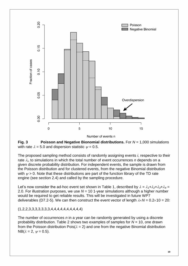
Fig. 3 Poisson and Negative Bionomial distributions. For N = 1,000 simulations

with rate = 5.0 and dispersion statistic = 0.5. The proposed sampling method consists of randomly assigning events i, respective to their

rate i, to simulations in which the total number of event occurrences n depends on a given discrete probability distribution. For independent events, the sample is drawn from the Poisson distribution and for clustered events, from the negative Binomial distribution

with > 0. Note that these distributions are part of the function library of the TD rate engine (see section 2.4) and called by the sampling procedure.

Let’s now consider the ad-hoc event set shown in Table 1, described by = 1+2+3+4 = 2.0. For illustration purposes, we use N = 10 1-year simulations although a higher number would be required to get reliable results. This will be investigated in future WP7

deliverables (D7.2-5). We can then construct the event vector of length N = 0.210 = 20: (1,2,2,3,3,3,3,3,3,3,4,4,4,4,4,4,4,4,4,4) The number of occurrences n in a year can be randomly generated by using a discrete probability distribution. Table 2 shows two examples of samples for N = 10, one drawn

from the Poisson distribution Pois( = 2) and one from the negative Binomial distribution

NB( = 2, = 0.5).

20

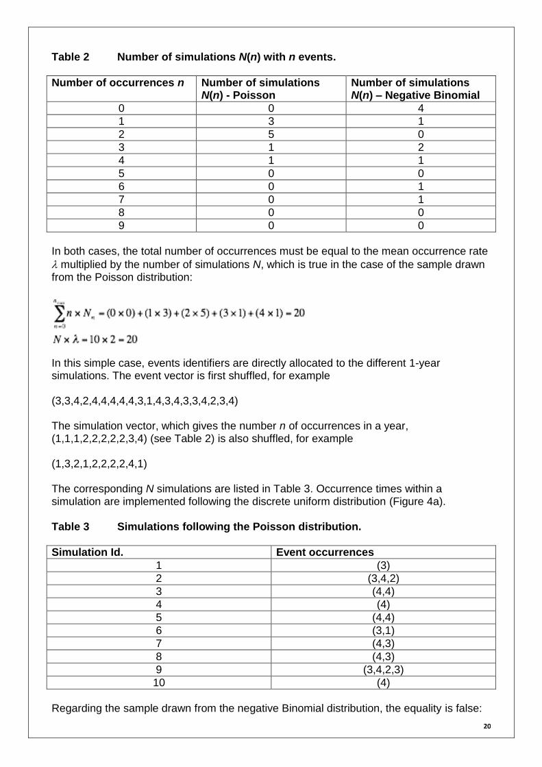
Table 2 Number of simulations N(n) with n events.

Number of occurrences n Number of simulations N(n) - Poisson

Number of simulations N(n) – Negative Binomial

0 0 4

1 3 1

2 5 0

3 1 2

4 1 1

5 0 0

6 0 1

7 0 1

8 0 0

9 0 0

In both cases, the total number of occurrences must be equal to the mean occurrence rate

multiplied by the number of simulations N, which is true in the case of the sample drawn from the Poisson distribution:

In this simple case, events identifiers are directly allocated to the different 1-year simulations. The event vector is first shuffled, for example (3,3,4,2,4,4,4,4,4,3,1,4,3,4,3,3,4,2,3,4) The simulation vector, which gives the number n of occurrences in a year, (1,1,1,2,2,2,2,2,3,4) (see Table 2) is also shuffled, for example (1,3,2,1,2,2,2,2,4,1) The corresponding N simulations are listed in Table 3. Occurrence times within a simulation are implemented following the discrete uniform distribution (Figure 4a). Table 3 Simulations following the Poisson distribution.

Simulation Id. Event occurrences

1 (3)

2 (3,4,2)

3 (4,4)

4 (4)

5 (4,4)

6 (3,1)

7 (4,3)

8 (4,3)

9 (3,4,2,3)

10 (4)

Regarding the sample drawn from the negative Binomial distribution, the equality is false:

21

In this case, there is an additional step, which consists of defining a new event vector composed of 24 events instead of 20, by a partition procedure. The stochastic event set is first partitioned into the interval (0,1) with each event Id. allocated to a subinterval proportional to its occurrence rate (Table 4). Then, the 24 events to be implemented are associated with a midpoint, which represents their relative position on the (0,1) interval. For each midpoint, there is a matching event Id., following the partition shown in Table 4. The new event vector and the intermediary calculations are given in Table 5. Table 4 Partitioning of stochastic events on (0,1) interval.

Event Id. Occurrence rate Conditional rate Partition

1 0.1 0.1/2 = 0.05 (0, 0.05)

2 0.2 0.2/2 = 0.10 (0.05, 0.15)

3 0.7 0.7/2 = 0.35 (0.15, 0.50)

4 1.0 1.0/2 = 0.50 (0.50, 1)

Table 5 Definition of the event vector of length 24.

Interval Midpoint Matching partition Matching event id.

(0, 1/24) 0.021 (0, 0.05) 1

(1/24, 2/24) 0.062 (0.05, 0.15) 2

(2/24, 3/24) 0.104 (0.05, 0.15) 2

(3/24, 4/24) 0.146 (0.05, 0.15) 2

(4/24, 5/24) 0.187 (0.15, 0.50) 3

(5/24, 6/24) 0.229 (0.15, 0.50) 3

(6/24, 7/24) 0.271 (0.15, 0.50) 3

(7/24, 8/24) 0.312 (0.15, 0.50) 3

(8/24, 9/24) 0.354 (0.15, 0.50) 3

(9/24, 10/24) 0.400 (0.15, 0.50) 3

(10/24, 11/24) 0.437 (0.15, 0.50) 3

(11/24, 12/24) 0.479 (0.15, 0.50) 3

(12/24, 13/24) 0.521 (0.50, 1) 4

(13/24, 14/24) 0.562 (0.50, 1) 4

(14/24, 15/24) 0.604 (0.50, 1) 4

(15/24, 16/24) 0.646 (0.50, 1) 4

(16/24, 17/24) 0.687 (0.50, 1) 4

(17/24, 18/24) 0.729 (0.50, 1) 4

(18/24, 19/24) 0.771 (0.50, 1) 4

(19/24, 20/24) 0.812 (0.50, 1) 4

(20/24, 21/24) 0.854 (0.50, 1) 4

(21/24, 22/24) 0.896 (0.50, 1) 4

(22/24, 23/24) 0.937 (0.50, 1) 4

(23/24, 1) 0.979 (0.50, 1) 4

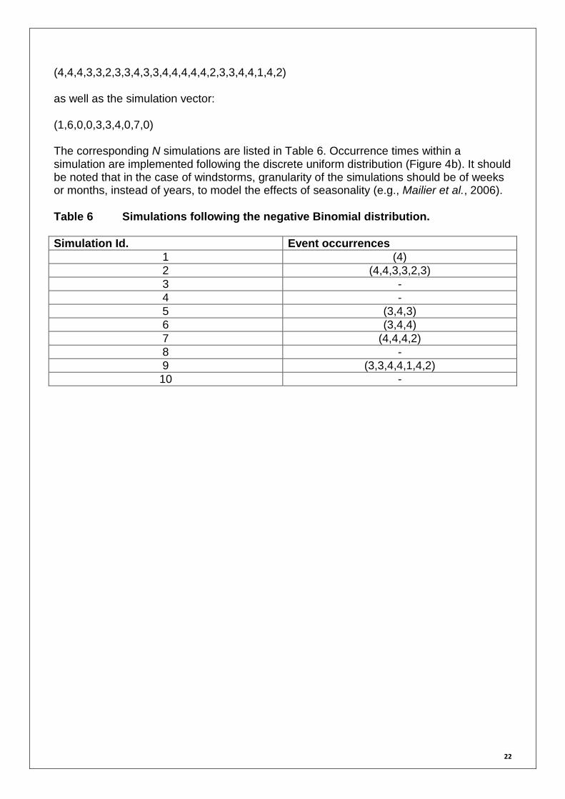
The method is then the same as described previously. The event vector is shuffled:

22

(4,4,4,3,3,2,3,3,4,3,3,4,4,4,4,4,2,3,3,4,4,1,4,2) as well as the simulation vector: (1,6,0,0,3,3,4,0,7,0) The corresponding N simulations are listed in Table 6. Occurrence times within a simulation are implemented following the discrete uniform distribution (Figure 4b). It should be noted that in the case of windstorms, granularity of the simulations should be of weeks or months, instead of years, to model the effects of seasonality (e.g., Mailier et al., 2006). Table 6 Simulations following the negative Binomial distribution.

Simulation Id. Event occurrences

1 (4)

2 (4,4,3,3,2,3)

3 -

4 -

5 (3,4,3)

6 (3,4,4)

7 (4,4,4,2)

8 -

9 (3,3,4,4,1,4,2)

10 -

23

Fig. 4 Event time series from different distributions. (a) From a Poisson distribution with occurrence rates from Table 1; (b) From a negative Binomial distribution

with occurrence rates from Table 1 and = 0.5.

24

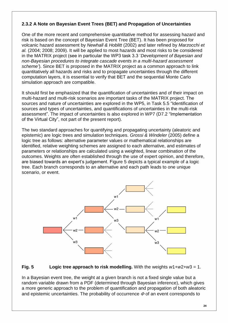
2.3.2 A Note on Bayesian Event Trees (BET) and Propagation of Uncertainties One of the more recent and comprehensive quantitative method for assessing hazard and risk is based on the concept of Bayesian Event Tree (BET). It has been proposed for volcanic hazard assessment by Newhall & Hoblitt (2002) and later refined by Marzocchi et al. (2004; 2008; 2009). It will be applied to most hazards and most risks to be considered in the MATRIX project (see in particular the WP3 task 3.3 ‘Development of Bayesian and non-Bayesian procedures to integrate cascade events in a multi-hazard assessment scheme’). Since BET is proposed in the MATRIX project as a common approach to link quantitatively all hazards and risks and to propagate uncertainties through the different computation layers, it is essential to verify that BET and the sequential Monte Carlo simulation approach are compatible. It should first be emphasized that the quantification of uncertainties and of their impact on multi-hazard and multi-risk scenarios are important tasks of the MATRIX project. The sources and nature of uncertainties are explored in the WP5, in Task 5.5 “Identification of sources and types of uncertainties, and quantifications of uncertainties in the multi-risk assessment”. The impact of uncertainties is also explored in WP7 (D7.2 “Implementation of the Virtual City”, not part of the present report). The two standard approaches for quantifying and propagating uncertainty (aleatoric and epistemic) are logic trees and simulation techniques. Grossi & Windeler (2005) define a logic tree as follows: alternative parameter values or mathematical relationships are identified, relative weighting schemes are assigned to each alternative, and estimates of parameters or relationships are calculated using a weighted, linear combination of the outcomes. Weights are often established through the use of expert opinion, and therefore, are biased towards an expert’s judgement. Figure 5 depicts a typical example of a logic tree. Each branch corresponds to an alternative and each path leads to one unique scenario, or event.

Fig. 5 Logic tree approach to risk modelling. With the weights w1+w2+w3 = 1. In a Bayesian event tree, the weight at a given branch is not a fixed single value but a random variable drawn from a PDF (determined through Bayesian inference), which gives a more generic approach to the problem of quantification and propagation of both aleatoric

and epistemic uncertainties. The probability of occurrence of an event corresponds to

25

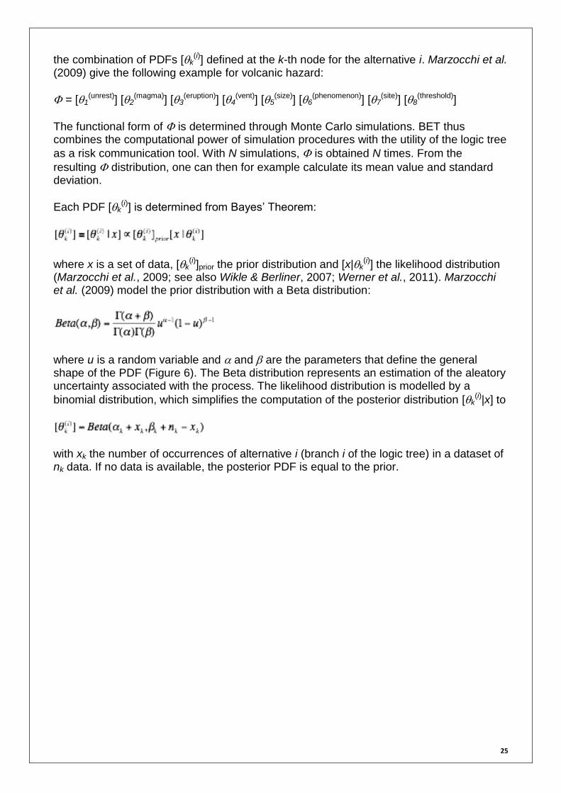
the combination of PDFs [k(i)] defined at the k-th node for the alternative i. Marzocchi et al.

(2009) give the following example for volcanic hazard:

= [1(unrest)] [2

(magma)] [3(eruption)] [4

(vent)] [5(size)] [6

(phenomenon)] [7(site)] [8

(threshold)]

The functional form of is determined through Monte Carlo simulations. BET thus combines the computational power of simulation procedures with the utility of the logic tree

as a risk communication tool. With N simulations, is obtained N times. From the

resulting distribution, one can then for example calculate its mean value and standard deviation.

Each PDF [k(i)] is determined from Bayes’ Theorem:

where x is a set of data, [k(i)]prior the prior distribution and [x|k

(i)] the likelihood distribution (Marzocchi et al., 2009; see also Wikle & Berliner, 2007; Werner et al., 2011). Marzocchi et al. (2009) model the prior distribution with a Beta distribution:

where u is a random variable and and are the parameters that define the general shape of the PDF (Figure 6). The Beta distribution represents an estimation of the aleatory uncertainty associated with the process. The likelihood distribution is modelled by a

binomial distribution, which simplifies the computation of the posterior distribution [k(i)|x] to

with xk the number of occurrences of alternative i (branch i of the logic tree) in a dataset of nk data. If no data is available, the posterior PDF is equal to the prior.

26

Fig. 6 Example of different Beta distributions. The solid, dashed and dotted

lines represent Beta(=2,=4), Beta(+ ) or Dirac’s distribution (0.33) and

Beta(=1,=1) or uniform distribution, respectively. Identical to Figure 10 of Marzocchi et al. (2009). One example of volcanic event, following the nomenclature of Marzocchi et al. (2009), could have the following probability of occurrence:

= [1(unrest: YES)] [2

(magma: YES)] [3(eruption: YES)] [4

(vent: no. 1)] [5(size: VEI = 4)] [6

(phenomenon: Tephra

fall)] [7(site: cell no. 1)] [8

(threshold: Tephra thickness)]

This event is defined via an 8-level logic tree with depending on the combination of the 8

PDFs [k], i.e., 8 different Beta distributions (some equal to the Dirac’s distribution, i.e., YES/NO choice). PDF selection for the Vesuvius volcano BET is given in Marzocchi et al. (2004). This event definition is different from the one used previously, where each event, in

an event table, is associated with one fixed occurrence rate (see Table 1). In the case a

BET is available, one could define the occurrence rate in the event table by the PDF , or

simply by the mean and standard deviation of . Figure 7 shows how an event table can be generated from a BET. In Figure 7a, the weight wk,i of alternative i at node k is

generated from the incomplete Beta function iBetak,i(k,i,k,i) for a random quantile q (0 ≤ q ≤ 1). In Figure 7b, each path of the logic tree defines one unique event, with a unique identifier and a unique intensity surface (e.g., Tephra fall of specific thickness at specific site).

27

Fig. 7 From a Bayesian event tree to an event table. (a) For each simulation, a weight w is generated from the incomplete Beta function for a random quantile q. (b) Id. (1,1).(2,3) is the Tephra event at site 1 with thickness 3. For each simulation, the weight w1,1 at k = 1, i = 1 is drawn from Beta(2,6) and weight w2,3 at k = 2, i = 3 from Beta(2,2). The event occurrence is described by the PDF of w = w1,1w2,3 defined from N simulations. Sampling procedures (section 2.3.1) would remain the same but for each simulation, the

event rate would be drawn from the corresponding event PDF, if available. The impact of rate uncertainty on losses will be investigated in the task 7.2 “Implementation and analysis of the Virtual City”. It should be noted that the BET framework is generic and is applied in the same way as for other hazards, by adding more branches to a same tree level, as well as for risk, by adding further levels to the tree (assets, vulnerability, etc.). BET methodologies for describing cascade phenomena are investigated in detail in WP3 of the MATRIX project. Since these are based on Monte Carlo simulations, we anticipate results from WP3 to be compatible with our simulation framework. Regarding the concept of Bayesian belief network (BBN), adopted by Aspinall et al. (2003) and to be implemented by ASPINALL in the MATRIX project, it shares the same philosophy as BET (Marzocchi et al., 2008) and is therefore not discussed here. 2.4 TIME-DEPENDENT RATE ENGINE CONCEPTUALIZATION The purpose of the TD rate engine is to implement rate changes due to correlations between events, so-called cascade or domino events. These correlations can be intra-hazard (e.g., an earthquake triggering another earthquake, a clustering of windstorm events) or inter-hazard (e.g., a volcanic eruption triggering an earthquake, an earthquake triggering a landslide). Earthquake/earthquake interaction is well established (see the review by King, 2007) as is windstorm clustering (e.g., Mailier et al., 2006; Vitolo et al., 2009) or earthquake/landslide triggering (e.g., Haugen & Kaynia, 2008; Nadim et al., 2006). While some evidence for earthquake/volcanic eruption interaction exists (e.g., Marzocchi, 2002; Hill et al., 2002), the

28

physical processes involved are not yet fully understood (see the review by Eggert & Walter, 2009). Nevertheless, with regards to the Naples test case, Mount Vesuvius has been shown to be associated with major earthquakes (e.g., Marzocchi et al., 1993), making earthquake/volcanic eruption interaction an additional key process to be implemented in the MATRIX multi-risk platform. Other typical interactions include tsunamis generated by earthquakes or landslides by heavy rains. Industrial accidents can also be triggered by a number of natural hazards (e.g., Marzocchi et al., 2009). The different hazards are studied in detail in WP2 and their potential interactions in WP3 of the MATRIX project. Basically, the TD rate engine is an interface between the stochastic event set database,

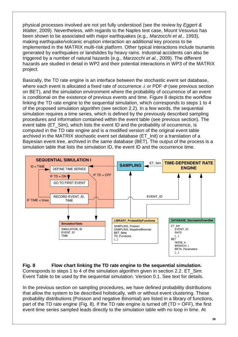
where each event is allocated a fixed rate of occurrence or PDF (see previous section on BET), and the simulation environment where the probability of occurrence of an event is conditional on the existence of previous events and time. Figure 8 depicts the workflow linking the TD rate engine to the sequential simulation, which corresponds to steps 1 to 4 of the proposed simulation algorithm (see section 2.2). In a few words, the sequential simulation requires a time series, which is defined by the previously described sampling procedures and information contained within the event table (see previous section). The event table (ET_Sim), which lists the event ID and the probability of occurrence, is computed in the TD rate engine and is a modified version of the original event table archived in the MATRIX stochastic event set database (ET_Init) or a translation of a Bayesian event tree, archived in the same database (BET). The output of the process is a simulation table that lists the simulation ID, the event ID and the occurrence time.

Fig. 8 Flow chart linking the TD rate engine to the sequential simulation. Corresponds to steps 1 to 4 of the simulation algorithm given in section 2.2. ET_Sim: Event Table to be used by the sequential simulation. Version 0.1. See text for details. In the previous section on sampling procedures, we have defined probability distributions that allow the system to be described holistically, with or without event clustering. These probability distributions (Poisson and negative Binomial) are listed in a library of functions, part of the TD rate engine (Fig. 8). If the TD rate engine is turned off (TD = OFF), the first event time series sampled leads directly to the simulation table with no loop in time. At

29

present, let’s consider time-dependency in the occurrence of individual events (section 2.4.1) and of trigger/target event couples (section 2.4.2). The procedures described below are illustrated using the earthquake case. Reference to other perils is made when necessary. 2.4.1 Implementation of Renewal Processes The recurrence of some individual events is best described by a time-dependent, or renewal process. This is for example the case of earthquakes: If an event has occurred on a fault, the probability of a second earthquake on the same fault (same event Id.) is close to zero immediately after the first occurrence. The probability then rises gradually through time due to constant loading on the fault. Therefore, if the occurrence time of the last event on a given fault is known (i.e., historical event), a renewal process should be directly implemented in step 1 of the simulation algorithm (i.e., definition of event time series). The earthquake renewal process can be described by different probability distributions. The most commonly used in time-dependent seismic hazard are the lognormal and Brownian Passage Time (BPT) distributions (e.g., Parsons, 2005). Other renewal processes include the Gamma and Weibull distributions, which have been proposed to be indicative of strong coupling between faults (Zöller & Hainzl, 2007).

The time-dependent probability on interval t is:

where f(t) is the probability density function (PDF) for the earthquake’s recurrence. The probability conditioned on the non-occurrence of the event prior to t is:

For illustration purposes, let’s only consider the lognormal distribution:

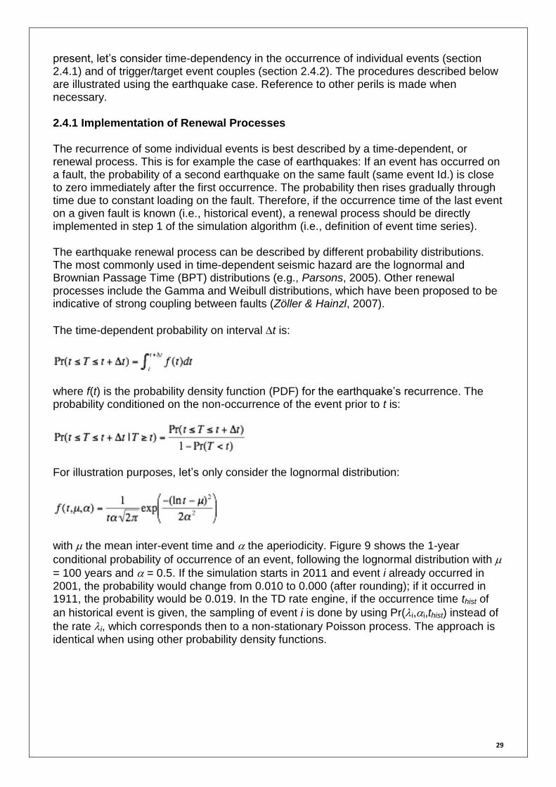
with the mean inter-event time and the aperiodicity. Figure 9 shows the 1-year

conditional probability of occurrence of an event, following the lognormal distribution with

= 100 years and = 0.5. If the simulation starts in 2011 and event i already occurred in 2001, the probability would change from 0.010 to 0.000 (after rounding); if it occurred in 1911, the probability would be 0.019. In the TD rate engine, if the occurrence time thist of

an historical event is given, the sampling of event i is done by using Pr(i,i,thist) instead of

the rate i, which corresponds then to a non-stationary Poisson process. The approach is identical when using other probability density functions.

30

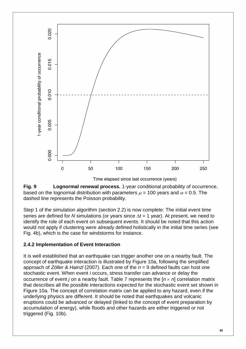
Fig. 9 Lognormal renewal process. 1-year conditional probability of occurrence,

based on the lognormal distribution with parameters = 100 years and = 0.5. The dashed line represents the Poisson probability. Step 1 of the simulation algorithm (section 2.2) is now complete: The initial event time

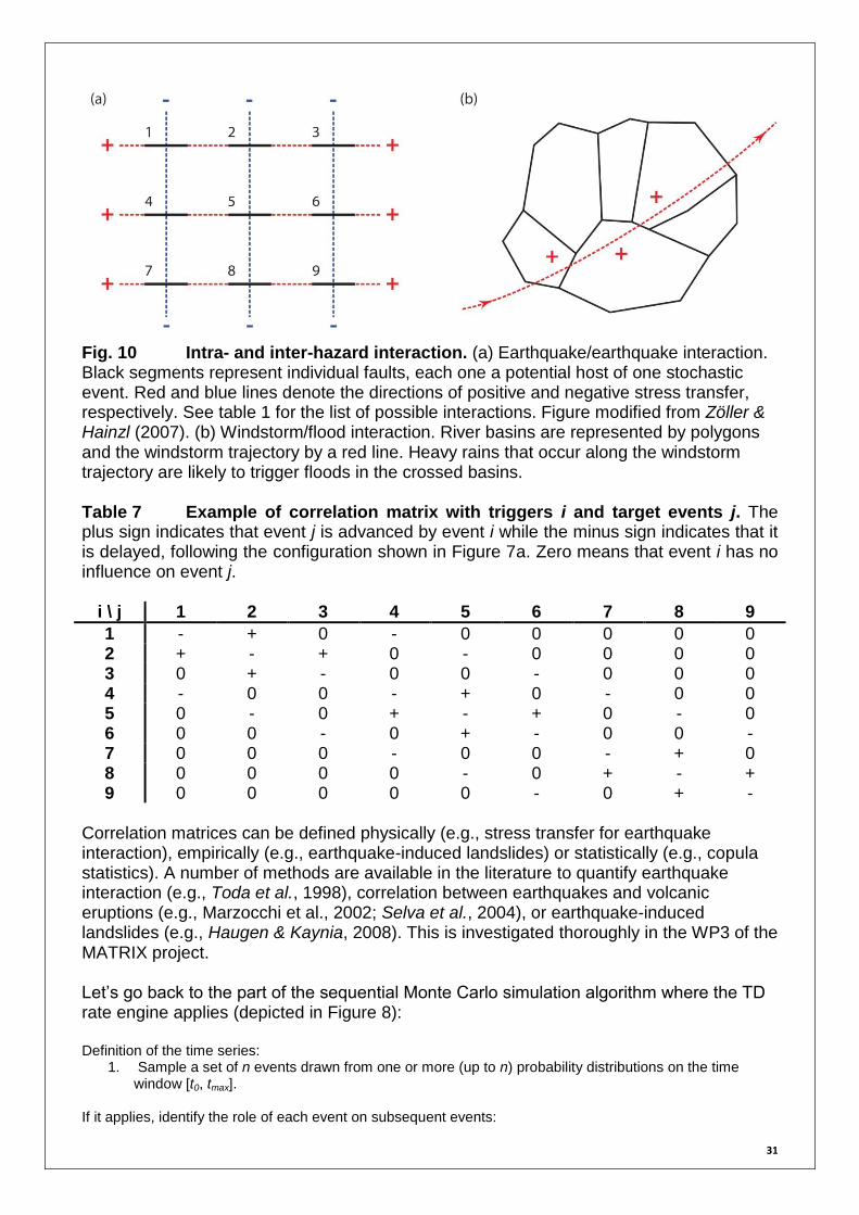
series are defined for N simulations (or years since t = 1 year). At present, we need to identify the role of each event on subsequent events. It should be noted that this action would not apply if clustering were already defined holistically in the initial time series (see Fig. 4b), which is the case for windstorms for instance. 2.4.2 Implementation of Event Interaction It is well established that an earthquake can trigger another one on a nearby fault. The concept of earthquake interaction is illustrated by Figure 10a, following the simplified approach of Zöller & Hainzl (2007). Each one of the n = 9 defined faults can host one stochastic event. When event i occurs, stress transfer can advance or delay the

occurrence of event j on a nearby fault. Table 7 represents the [n n] correlation matrix that describes all the possible interactions expected for the stochastic event set shown in Figure 10a. The concept of correlation matrix can be applied to any hazard, even if the underlying physics are different. It should be noted that earthquakes and volcanic eruptions could be advanced or delayed (linked to the concept of event preparation by accumulation of energy), while floods and other hazards are either triggered or not triggered (Fig. 10b).

31

Fig. 10 Intra- and inter-hazard interaction. (a) Earthquake/earthquake interaction. Black segments represent individual faults, each one a potential host of one stochastic event. Red and blue lines denote the directions of positive and negative stress transfer, respectively. See table 1 for the list of possible interactions. Figure modified from Zöller & Hainzl (2007). (b) Windstorm/flood interaction. River basins are represented by polygons and the windstorm trajectory by a red line. Heavy rains that occur along the windstorm trajectory are likely to trigger floods in the crossed basins. Table 7 Example of correlation matrix with triggers i and target events j. The plus sign indicates that event j is advanced by event i while the minus sign indicates that it is delayed, following the configuration shown in Figure 7a. Zero means that event i has no influence on event j.

i \ j 1 2 3 4 5 6 7 8 9

1 - + 0 - 0 0 0 0 0 2 + - + 0 - 0 0 0 0 3 0 + - 0 0 - 0 0 0 4 - 0 0 - + 0 - 0 0 5 0 - 0 + - + 0 - 0 6 0 0 - 0 + - 0 0 - 7 0 0 0 - 0 0 - + 0 8 0 0 0 0 - 0 + - + 9 0 0 0 0 0 - 0 + -

Correlation matrices can be defined physically (e.g., stress transfer for earthquake interaction), empirically (e.g., earthquake-induced landslides) or statistically (e.g., copula statistics). A number of methods are available in the literature to quantify earthquake interaction (e.g., Toda et al., 1998), correlation between earthquakes and volcanic eruptions (e.g., Marzocchi et al., 2002; Selva et al., 2004), or earthquake-induced landslides (e.g., Haugen & Kaynia, 2008). This is investigated thoroughly in the WP3 of the MATRIX project. Let’s go back to the part of the sequential Monte Carlo simulation algorithm where the TD rate engine applies (depicted in Figure 8): Definition of the time series:

1. Sample a set of n events drawn from one or more (up to n) probability distributions on the time window [t0, tmax].

If it applies, identify the role of each event on subsequent events:

32

2. Go to ti, the occurrence time of the first event in the time window chronology. Record event i. 3. Apply the TD rate engine to update all probabilities of occurrence or their distributions, conditional

on event i and ti. 4. Repeat steps 1, 2 and 3 with t0 = ti until ti < tmax.

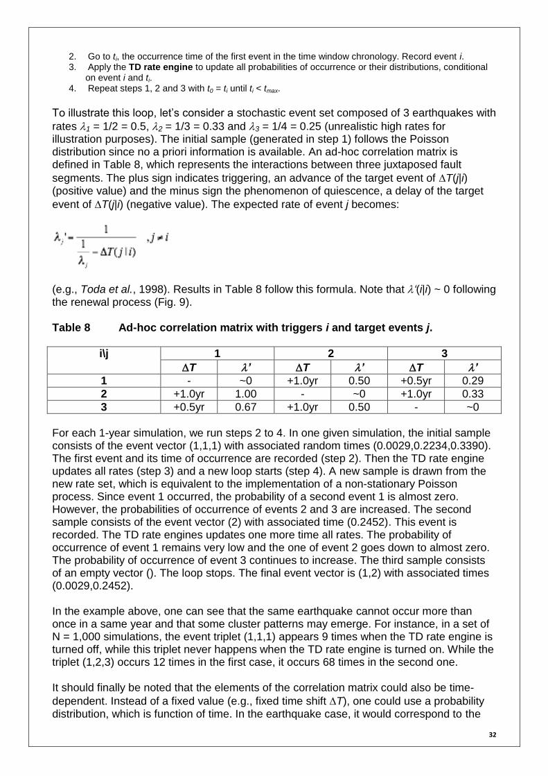
To illustrate this loop, let’s consider a stochastic event set composed of 3 earthquakes with

rates 1 = 1/2 = 0.5, 2 = 1/3 = 0.33 and 3 = 1/4 = 0.25 (unrealistic high rates for illustration purposes). The initial sample (generated in step 1) follows the Poisson distribution since no a priori information is available. An ad-hoc correlation matrix is defined in Table 8, which represents the interactions between three juxtaposed fault

segments. The plus sign indicates triggering, an advance of the target event of T(j|i) (positive value) and the minus sign the phenomenon of quiescence, a delay of the target

event of T(j|i) (negative value). The expected rate of event j becomes:

(e.g., Toda et al., 1998). Results in Table 8 follow this formula. Note that ‘(i|i) ~ 0 following the renewal process (Fig. 9). Table 8 Ad-hoc correlation matrix with triggers i and target events j.

i\j 1 2 3

T ’ T ’ T ’ 1 - ~0 +1.0yr 0.50 +0.5yr 0.29

2 +1.0yr 1.00 - ~0 +1.0yr 0.33

3 +0.5yr 0.67 +1.0yr 0.50 - ~0

For each 1-year simulation, we run steps 2 to 4. In one given simulation, the initial sample consists of the event vector (1,1,1) with associated random times (0.0029,0.2234,0.3390). The first event and its time of occurrence are recorded (step 2). Then the TD rate engine updates all rates (step 3) and a new loop starts (step 4). A new sample is drawn from the new rate set, which is equivalent to the implementation of a non-stationary Poisson process. Since event 1 occurred, the probability of a second event 1 is almost zero. However, the probabilities of occurrence of events 2 and 3 are increased. The second sample consists of the event vector (2) with associated time (0.2452). This event is recorded. The TD rate engines updates one more time all rates. The probability of occurrence of event 1 remains very low and the one of event 2 goes down to almost zero. The probability of occurrence of event 3 continues to increase. The third sample consists of an empty vector (). The loop stops. The final event vector is (1,2) with associated times (0.0029,0.2452). In the example above, one can see that the same earthquake cannot occur more than once in a same year and that some cluster patterns may emerge. For instance, in a set of N = 1,000 simulations, the event triplet (1,1,1) appears 9 times when the TD rate engine is turned off, while this triplet never happens when the TD rate engine is turned on. While the triplet (1,2,3) occurs 12 times in the first case, it occurs 68 times in the second one. It should finally be noted that the elements of the correlation matrix could also be time-

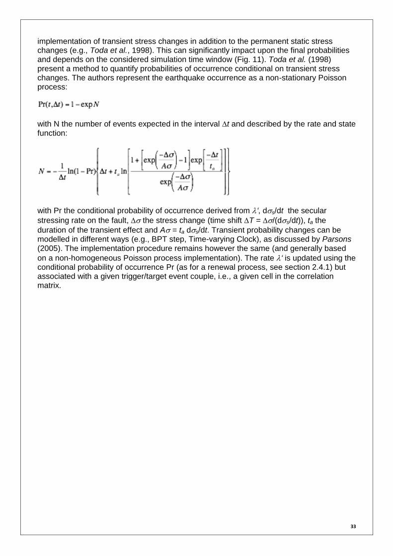
dependent. Instead of a fixed value (e.g., fixed time shift T), one could use a probability distribution, which is function of time. In the earthquake case, it would correspond to the

33

implementation of transient stress changes in addition to the permanent static stress changes (e.g., Toda et al., 1998). This can significantly impact upon the final probabilities and depends on the considered simulation time window (Fig. 11). Toda et al. (1998) present a method to quantify probabilities of occurrence conditional on transient stress changes. The authors represent the earthquake occurrence as a non-stationary Poisson process:

with N the number of events expected in the interval t and described by the rate and state function:

with Pr the conditional probability of occurrence derived from ‘, ds/dt the secular

stressing rate on the fault, the stress change (time shift T = /(ds/dt)), ta the

duration of the transient effect and A = ta ds/dt. Transient probability changes can be modelled in different ways (e.g., BPT step, Time-varying Clock), as discussed by Parsons (2005). The implementation procedure remains however the same (and generally based

on a non-homogeneous Poisson process implementation). The rate ‘ is updated using the conditional probability of occurrence Pr (as for a renewal process, see section 2.4.1) but associated with a given trigger/target event couple, i.e., a given cell in the correlation matrix.

34

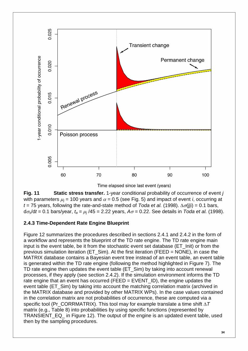
Fig. 11 Static stress transfer. 1-year conditional probability of occurrence of event j

with parameters j = 100 years and = 0.5 (see Fig. 5) and impact of event i, occurring at

t = 75 years, following the rate-and-state method of Toda et al. (1998). (j|i) = 0.1 bars,

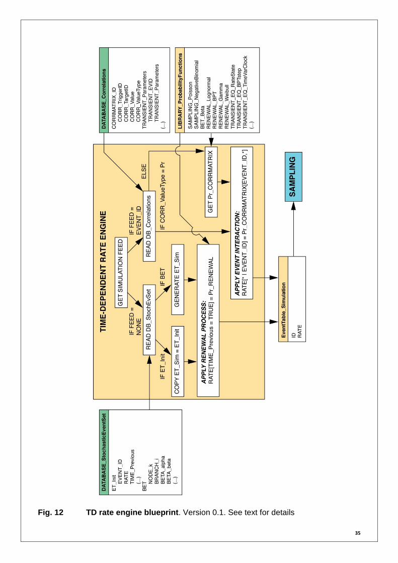
ds/dt = 0.1 bars/year, ta = j /45 = 2.22 years, A = 0.22. See details in Toda et al. (1998). 2.4.3 Time-Dependent Rate Engine Blueprint Figure 12 summarizes the procedures described in sections 2.4.1 and 2.4.2 in the form of a workflow and represents the blueprint of the TD rate engine. The TD rate engine main input is the event table, be it from the stochastic event set database (ET_Init) or from the previous simulation iteration (ET_Sim). At the first iteration (FEED = NONE), in case the MATRIX database contains a Bayesian event tree instead of an event table, an event table is generated within the TD rate engine (following the method highlighted in Figure 7). The TD rate engine then updates the event table (ET_Sim) by taking into account renewal processes, if they apply (see section 2.4.2). If the simulation environment informs the TD rate engine that an event has occurred (FEED = EVENT_ID), the engine updates the event table (ET_Sim) by taking into account the matching correlation matrix (archived in the MATRIX database and provided by other MATRIX WPs). In the case values contained in the correlation matrix are not probabilities of occurrence, these are computed via a

specific tool (Pr_CORRMATRIX). This tool may for example translate a time shift T matrix (e.g., Table 8) into probabilities by using specific functions (represented by TRANSIENT_EQ_ in Figure 12). The output of the engine is an updated event table, used then by the sampling procedures.

35

Fig. 12 TD rate engine blueprint. Version 0.1. See text for details

36

2.5 TIME-DEPENDENT VULNERABILITY ENGINE CONCEPTUALIZATION The damage module, as depicted in Figure 1 and briefly described in section 2.1.2, computes the mean damage ratio (MDR) from a vulnerability function, which depends on hazard intensity and on the capacity of the asset to withstand the impact. The purpose of the TD vulnerability engine is to implement vulnerability curves, which are dependent on the occurrence of previous events, on time, or on both. In the scope of the MATRIX project, dynamic vulnerability includes both physical and functional (socio-economic) aspects:

Time-dependent physical vulnerability: The impact of successive events on the structure of a building has been studied in intra-hazard cases such as seismic sequences (e.g., Jalayer et al., 2010) as well inter-hazard case such as volcanic eruption/earthquake coupling (e.g., Baratta et al., 2003). In the first example, it is the repetitive shaking that affects the structural resistance of a building, while in the second, it is the volcanic ash load that increases the vulnerability. This field of engineering research is recent and it hasn’t led to the definition of a fully time-dependent physical vulnerability. This is, however, investigated in WP4 of the MATRIX project, specifically by considering the impact of repeated seismic events on the physical vulnerability of a given building typology. It should be added that the aging of structures has an impact on vulnerability over time (e.g., Rao et al., 2010). Here, vulnerability depends directly on time, while in the other cases, it depends on previous events and thus indirectly on time. There is, however, no current plan to take this aspect into account in WP4 (pers. comm., August 2011, Arnaud Reveillère).

Time-dependent functional vulnerability: While the physical damage of a key infrastructure leads to direct losses, the alteration of its function may lead to additional, indirect losses. Key infrastructures are utility networks (water, electricity, transportation), emergency services (hospitals, fire and police departments) but also industries (a failure leading to business interruption). Systemic vulnerability, based on the principle of cascade failures within a system, takes into account all the interdependencies in the system. For instance, a hospital cannot function without electricity or water (e.g., Marti et al., 2008). Thanks to many redundancies and capacity upgrades through time, most key infrastructures can cope to some extent with a disaster. The event may weaken the operating margin of the system without altering its functions. However the occurrence of a second event may lead to a break down of system due to its already degraded running mode. Specific scenarios are evaluated in WP4 (and in WP6 to include decision support strategies).

Basically, the TD vulnerability engine is an interface between the simulation environment where event time series, which may include cluster patterns, are fixed and the damage engine where the MDR is computed. Figure 13 depicts the corresponding workflow, including the subsequent loss computation (i.e., loss and TD exposure engines), which all together correspond to steps 5 to 9 of the proposed simulation algorithm (see section 2.2). Here, a MDR is computed for each asset location considered for each event pre-defined in the time series (see sections 2.3 and 2.4 for their generation). Damage computation requires a specific vulnerability curve, which is provided by the TD vulnerability engine after identifying possible time-dependent processes, conditional on previous events (or on time). This workflow includes the stochastic event database, the asset database and a library of vulnerability functions. At the end of the process, the simulation table is updated

37

with the MDR and loss (and uncertainties if required), which are linked to each event of the table.

Fig. 13 Flow chart linking the TD vulnerability engine to the sequential simulation. Corresponds to steps 5 to 9 of the simulation algorithm given in section 2.2. Version 0.1. See text for details. 2.5.1 Time-Dependent Vulnerability Engine Blueprint The loss engine of the proposed MATRIX platform is expected to compute direct losses, as described in section 2.1.3 (and possibly some basic indirect losses – to be defined by the WP5 and WP6 of the MATRIX project). However a module for socio-economic impact should be juxtaposed to the loss module, as implementation of infrastructure networks requires its own logical unit (see next section). As a consequence, the TD vulnerability engine, as depicted in Figure 13, will consider physical vulnerability only. The role of the TD vulnerability engine is to call specific vulnerability functions for the damage engine. These functions are part of a vulnerability function library, which should be provided by WP2 (general data gathering) and by WP4 (time-dependent vulnerability) of the MATRIX project. Each vulnerability curve is either described by a table or a mathematical function. Other attributes include the peril and the building parameters (especially the construction class) for which the curve is defined. An additional attribute, key to the TD engine, is whether the vulnerability is latent or time-dependent. In the second case, additional information is required in the library about the prior (event identifier or time). It should be noted that although WP4 does not plan to consider any direct link between vulnerability and time, it is still implemented in the engine to build a

38

comprehensive time-dependent framework for possible future studies in which vulnerability curves based on structural aging would be provided. It is anticipated that WP4 will provide a limited number of time-dependent vulnerability curves due to the cumbersome engineering requirements in generating them. This is the case for the BRGM study case, which will focus on vulnerability dependency to seismic sequences, for one specific building type (pers. comm., August 2011, Arnaud Reveillère). Regarding the AMRA study case, the vulnerability curves for earthquakes and their dependency to volcanic ash load will be generated from an ad-hoc methodology (pers. comm., July 2011, Jacopo Selva). This is similar to the concept of heuristic databases developed for the Virtual City (section 2.6). In the case that no time-dependent vulnerability curve is available from the library, time-dependent vulnerability could be turned off or a specific curve used as a generic input to other building construction classes. This approach is discussed in section 2.6. Figure 14 represents the workflow or blueprint of the TD (physical) vulnerability engine and damage engine. The TD engine gets the time series directly from the simulation table generated from the first part of the sequential simulation environment and the time increment i from the second part of the simulation environment. The algorithm that forms the TD engine is based on the action: identify attributes / retrieve matching vulnerability curve. Attributes include the peril type (PERIL, which should be part of the event ID description), the building attributes (e.g., BUILDING_ConstructionType from the asset database) and if the vulnerability is conditional on previous events (TD_Type = LATENT or TD). Although structural aging is considered in the workflow, it might not be made active in the MATRIX project. This algorithm is repeated for each asset location (PORTFOLIO_Asset) considered in the region of interest (this loop in space is not represented in Figure 14 for the sake of simplicity). The TD engine provides the vulnerability curve, time-dependent or not, to the damage engine. Other data propagate to the damage engine, such as the event ID from the simulation table, to retrieve the matching hazard intensity surface from the stochastic event set database (INTENSITY_ValueXY). Hazard footprints are commonly provided in grid format while assets are defined by polygons (GIS_Polygon). To match one intensity value per asset, an aggregation procedure must be added to the damage engine. This procedure will be defined in Build v. 1.x. The core of the damage engine computes the MDR for each event of the time series, using the intensity value at the asset location (INTENSITY_ValueAsset) and the vulnerability curve provided by the TD engine. The MDR is then copied to the simulation table (MDR_ValueAsset).

39

Fig. 14 TD (physical) vulnerability and damage engines blueprint. Version 0.1. See text for details.

40

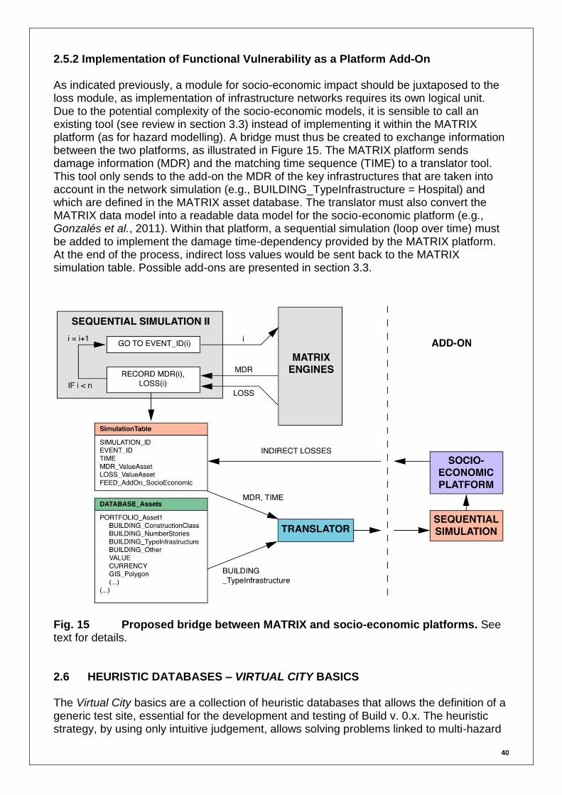
2.5.2 Implementation of Functional Vulnerability as a Platform Add-On As indicated previously, a module for socio-economic impact should be juxtaposed to the loss module, as implementation of infrastructure networks requires its own logical unit. Due to the potential complexity of the socio-economic models, it is sensible to call an existing tool (see review in section 3.3) instead of implementing it within the MATRIX platform (as for hazard modelling). A bridge must thus be created to exchange information between the two platforms, as illustrated in Figure 15. The MATRIX platform sends damage information (MDR) and the matching time sequence (TIME) to a translator tool. This tool only sends to the add-on the MDR of the key infrastructures that are taken into account in the network simulation (e.g., BUILDING_TypeInfrastructure = Hospital) and which are defined in the MATRIX asset database. The translator must also convert the MATRIX data model into a readable data model for the socio-economic platform (e.g., Gonzalés et al., 2011). Within that platform, a sequential simulation (loop over time) must be added to implement the damage time-dependency provided by the MATRIX platform. At the end of the process, indirect loss values would be sent back to the MATRIX simulation table. Possible add-ons are presented in section 3.3.

Fig. 15 Proposed bridge between MATRIX and socio-economic platforms. See text for details. 2.6 HEURISTIC DATABASES – VIRTUAL CITY BASICS The Virtual City basics are a collection of heuristic databases that allows the definition of a generic test site, essential for the development and testing of Build v. 0.x. The heuristic strategy, by using only intuitive judgement, allows solving problems linked to multi-hazard

41

and multi-risk modelling and to define guidelines for more sophisticated subsequent works. This approach also forms a robust foundation for sensitivity analyses where the range of tested parameters must be scientifically credible. Finally, a non-heuristic approach would be impractical here, since available data for hazard, vulnerability, or exposure are rather incomplete and yet require important efforts to be retrieved (note that data gathering for the three MATRIX test sites is part of the WP2). Incomplete data may prevent a number of analyses while the addition of some heuristic data avoids such an issue. These datasets may be characterized by high epistemic uncertainties, but these could be reduced with more and better data in the future. It should, however, be noted that while the Virtual City can suggest the theoretical benefits of multi-risk assessment for decision support, identifying their real-world practicality will require the study of real test sites where all aspects of multi-hazard and multi-risk are together taken into account (e.g., Naples, French West Indies and Cologne in the MATRIX project). The proposed heuristic databases are non-exhaustive and are only defined in this section to generate a specific scenario that allows us to test all the TD engines defined in Build v. 0.x, i.e.:

Time-dependent rate engine (Figure 12).

Time-dependent vulnerability engine (Figure 14).

Time-dependent exposure engine. Since the TD engines are defined in a generic way, any hazard could be applied to test their functionality. For now we focus on earthquake hazard, as its implementation in risk models is already well established, the relevant data are easily accessible and time-dependent processes are numerous. Below are presented different methodologies to generate a generic earthquake multi-risk Virtual City scenario from heuristic databases. Data to assess are:

Hazard - Earthquake definition (rate, magnitude, location)

Hazard - Earthquake intensity surfaces (e.g., PGA)

Vulnerability curves (e.g., damage to buildings)

Exposure (e.g., economical)

Parameters describing time-dependent processes 2.6.1 Data Simulation for a Generic Time-Dependent Earthquake Scenario Table 9 describes some simple mathematical relationships to describe hazard, vulnerability, exposure and time-dependent processes holistically. It should be noted that more sophisticated formulations exist and could replace the basic ones presented in Table 9 if necessary.

42

Table 9 Simple mathematical relationships used to describe earthquake hazard, vulnerability, exposure and time-dependent processes holistically.

Hazard - Earthquake rate and magnitude An earthquake stochastic set can be constructed from the Gutenberg-Richter law (Gutenberg & Richter, 1944).

Parameters: a, b (usually = 1)

Hazard - Earthquake intensity Seismic intensity attenuation functions are defined empirically and depend mostly on the source mechanism and the ground conditions (e.g., USGS, 1996). Here is one general form example (Ambraseys et al., 1996):

Parameters: magnitude M, r distance to source, d horizontal distance, h source depth

Vulnerability Vulnerability curves can be assumed to be lognormal in shape (e.g., Yamaguchi & Yamazachi, 2000).

Parameters: mean , standard deviation

Exposure The frequency-population size of cities is governed by a power-law (e.g., Newman, 2005). For a region with an homogenous repartition of goods, economical value can be assumed linearly proportional to the population size P.

43

Parameters: a, b (= 1, Newman, 2005)

Time-dependent rate A clustered time series can be sampled from the negative Binomial distribution (see section 2.3.1) or from other probability distributions (see section 2.4).

Parameters: rate , dispersion

Time-dependent vulnerability Increase in vulnerability can be simulated by

decreasing the value of log(), in agreement with shapes obtained from more complex computations (e.g., Rao et al., 2010).

All the information required for a basic time-dependent earthquake scenario is available from Table 9. Let’s now define a stochastic event set based on a 3-fault system, as shown in Figure 16a. The 3-fault configuration (parallel fault segments) makes each fault event a potential trigger of events on the 2 other faults, whether it is in a dip-slip or strike-slip environment (e.g., King, 2007). While this example is a generic one, it is topologically similar to earthquake clustering, which can be expected in different regions of Europe, including Italy (Apennines normal fault system, Chiarabba et al., 2011) or Portugal for instance (Muir-Wood & Mignan, 2009). Each fault segment has a fixed length of 20 km, which may cause a magnitude 6.5 event (Wells & Coppersmith, 1994). Each fault can be subdivided into 10 km and 5 km sub-segments to accommodate smaller events of magnitude 6.0 and 5.5 respectively. The list of events is given in the stochastic event table of Table 10. Rates by magnitude are defined from the Gutenberg-Richter law with parameters a = 5 and b = 1. Rates are then distributed into the events of the same magnitude. It should be noted that any event of the stochastic event set has no significance outside of this specific set. Using the attenuation relationship of Ambraseys et al. (1996) (with C1 = -1.39, C2 = 0.266, C3 = 0, C4 = -0.922, h0 = 3.5 km, see Table 9), we can compute the PGA footprint for each stochastic event of Table 10 as shown in Figure 16b.

44

Fig. 16 3-fault system for the Virtual City scenario. (a) Region setup with fault segments A, B and C. (b) Intensity footprints (PGA) for segment A and sub-segments A1 and A1a. Table 10 Stochastic event table for the Virtual City scenario.

Event ID Fault segment Magnitude Rate

EQ1 A 6.5 0.03/3 = 0.01

EQ2 A1 6.0 0.10/6 = 0.02

EQ3 A2 6.0 0.10/6 = 0.02

EQ4 A1a 5.5 0.32/12 = 0.03

EQ5 A1b 5.5 0.32/12 = 0.03

EQ6 A2a 5.5 0.32/12 = 0.03

EQ7 A2b 5.5 0.32/12 = 0.03

EQ8 B 6.5 0.03/3 = 0.01

EQ9 B1 6.0 0.10/6 = 0.02

EQ10 B2 6.0 0.10/6 = 0.02

EQ11 B1a 5.5 0.32/12 = 0.03

EQ12 B1b 5.5 0.32/12 = 0.03

EQ13 B2a 5.5 0.32/12 = 0.03

EQ14 B2b 5.5 0.32/12 = 0.03

EQ15 C 6.5 0.03/3 = 0.01

EQ16 C1 6.0 0.10/6 = 0.02

EQ17 C2 6.0 0.10/6 = 0.02

EQ18 C1a 5.5 0.32/12 = 0.03

EQ19 C1b 5.5 0.32/12 = 0.03

EQ20 C2a 5.5 0.32/12 = 0.03

EQ21 C2b 5.5 0.32/12 = 0.03

45

The exposure dataset is defined as a list of cities of different population size, following a power-law frequency-size distribution (see Table 9, Newman, 2005). With a = 6 and b = 1, we get 1 city of 1 million inhabitants, 10 of 100,000 inhabitants and 100 of 10,000 inhabitants. Let’s assume that each household counts 3 individuals and is valued at 300,000 Euros. It leads to an economic exposure composed of 1 city valued at 100 billions Euros, 10 at 10 billions Euros and 100 at 1 billion Euros. This approach is crude but is a first step to define an exposure dataset. The set of 111 cities is randomly distributed in

space in an area 100 km 100 km (population density of 300/km2), superimposed to the fault map (Figure 17). All buildings are considered to be of the same construction type,

characterized by a vulnerability function of a lognormal form with = log(0.4) and = 1/8 (see Table 9).

Fig. 17 Exposure spatial distribution for the Virtual City scenario. Cities are randomly distributed in space. Different time-dependent modelling options are possible for the generic earthquake scenario, by turning on or off the different TD engines. The first possibility is to simulate earthquake risk in a standard way with all TD engines turned off and the time series drawn from the Poisson distribution (see section 2.3.1). As the main purpose of the MATRIX project is to identify the impact of interdependencies, the Poisson model can first be compared to a clustering model, in which time series are drawn from the negative Binomial

distribution (in our scenario with = 2.0 to amplify clustering). Figure 18 shows the exceedance probability (EP) curves for both models. Here losses are defined as the aggregate losses per year to best identify the role of clustering on risk. The role of clustering on maximum losses per year should also be investigated; a thorough investigation of the impact of time-dependent processes on risk is part of WP5 of the MATRIX project.

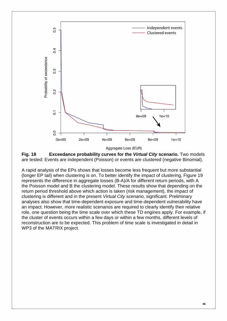
46

Fig. 18 Exceedance probability curves for the Virtual City scenario. Two models are tested: Events are independent (Poisson) or events are clustered (negative Binomial). A rapid analysis of the EPs shows that losses become less frequent but more substantial (longer EP tail) when clustering is on. To better identify the impact of clustering, Figure 19 represents the difference in aggregate losses (B-A)/A for different return periods, with A the Poisson model and B the clustering model. These results show that depending on the return period threshold above which action is taken (risk management), the impact of clustering is different and in the present Virtual City scenario, significant. Preliminary analyses also show that time-dependent exposure and time-dependent vulnerability have an impact. However, more realistic scenarios are required to clearly identify their relative role, one question being the time scale over which these TD engines apply. For example, if the cluster of events occurs within a few days or within a few months, different levels of reconstruction are to be expected. This problem of time scale is investigated in detail in WP3 of the MATRIX project.

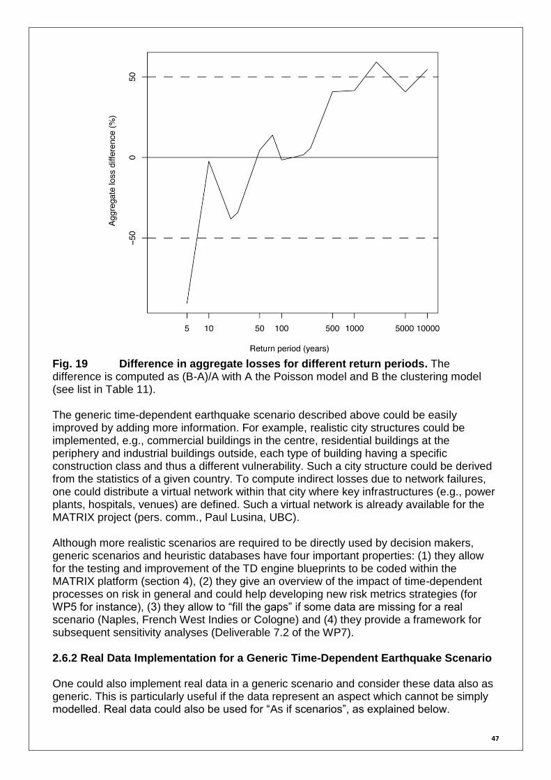
47

Fig. 19 Difference in aggregate losses for different return periods. The difference is computed as (B-A)/A with A the Poisson model and B the clustering model (see list in Table 11). The generic time-dependent earthquake scenario described above could be easily improved by adding more information. For example, realistic city structures could be implemented, e.g., commercial buildings in the centre, residential buildings at the periphery and industrial buildings outside, each type of building having a specific construction class and thus a different vulnerability. Such a city structure could be derived from the statistics of a given country. To compute indirect losses due to network failures, one could distribute a virtual network within that city where key infrastructures (e.g., power plants, hospitals, venues) are defined. Such a virtual network is already available for the MATRIX project (pers. comm., Paul Lusina, UBC). Although more realistic scenarios are required to be directly used by decision makers, generic scenarios and heuristic databases have four important properties: (1) they allow for the testing and improvement of the TD engine blueprints to be coded within the MATRIX platform (section 4), (2) they give an overview of the impact of time-dependent processes on risk in general and could help developing new risk metrics strategies (for WP5 for instance), (3) they allow to “fill the gaps” if some data are missing for a real scenario (Naples, French West Indies or Cologne) and (4) they provide a framework for subsequent sensitivity analyses (Deliverable 7.2 of the WP7). 2.6.2 Real Data Implementation for a Generic Time-Dependent Earthquake Scenario One could also implement real data in a generic scenario and consider these data also as generic. This is particularly useful if the data represent an aspect which cannot be simply modelled. Real data could also be used for “As if scenarios”, as explained below.

48

The ShakeMap atlas (see review in section 3.2.1) provides hazard intensity footprints of historical earthquakes, worldwide. It also implicitly includes time series where clustered events are present. Figure 20 shows two examples: (a) the 1997 Umbria-Marche, Italy, earthquake sequence with foreshock, mainshock and aftershocks, with magnitudes ranging from 5.3 to 6.0 and (b) the 1999 Izmit / Duzce, Turkey, large earthquake doublet with magnitudes 7.6 and 7.2, respectively. Other event clusters can easily be found in the ShakeMap atlas. These examples could directly be used as pre-defined time series in the simulation table, as shown in Table 11.

Fig. 20 ShakeMap PGA footprints of historical cascade events. (a) The 1997 Umbria-Marche, Italy, earthquake sequence with foreshock, mainshock and three aftershocks (magnitude range 5.3-6.0); (b) The 1999 Izmit / Duzce, Turkey, large earthquake doublet (magnitude range 7.2-7.6). Raw data from http://earthquake.usgs.gov/earthquakes/shakemap/. Table 11 Example of a simulation table based on real earthquake sequences. Sequences as defined in Figure 20.

SIMULATION_ID EVENT_ID TIME

1_UMBRIAMARCHE EQ_FORESHOCK1_M5,7 25.09.1997, 00:33UTC

1_UMBRIAMARCHE EQ_MAINSHOCK_M6,0 25.09.1997, 09:40UTC

1_UMBRIAMARCHE EQ_AFTERSHOCK1_M5,3 03.10.1997, 08:55UTC

1_UMBRIAMARCHE EQ_AFTERSHOCK2_M5,5 06.10.1997, 23:25UTC

1_UMBRIAMARCHE EQ_AFTERSHOCK3_M5,9 14.10.1997, 15:23UTC

2_IZMITDUZCE EQ_MAINSHOCK1_M7,6 17.08.1999, 00:01UTC

2_IZMITDUZCE EQ_MAINSHOCK2_M7,2 12.11.1999, 16:57UTC

One can thus construct a simulation table based on real clusters of events with matching hazard footprints. These can then be shifted in time (reproduction of an historical scenario) or to other locations. For instance, one could define the “what if the Umbria-Marche earthquake sequence occurred in Naples?” scenario or “what if the Izmit/Duzce earthquake doublet occurred 100 km more west, near Istanbul?” scenario. Of course,

49

these scenarios must be plausible, depending on the known hazard conditions at the studied site. Possibilities are multiple and should be defined by the different MATRIX partners. 2.7 LESSONS LEARNED AND GUIDELINES FOR BUILD v. 1.x The sketch of multi-risk modelling (Build v. 0.x) presented in section 2 provides basic guidelines to construct the MATRIX multi-risk platform (Build v. 1.x, section 4):

The simulation approach: It will form the core of the MATRIX platform. Although it has not been verified in Build v. 0.x, it is anticipated that the two loops on time (parts I and II of the sequential Monte Carlo simulation algorithm, section 2.2) may be computationally intensive.

TD engines: The workflow and the engine blueprints are provided by Build v. 0.x and can be directly translated into a programming language. Some R codes are already available and they could be integrated into the platform if this is considered a good option.

Other tools: In developing the multi-risk framework, the need for additional tools has emerged (represented in blue in the different blueprints). These include: (1) a sampling tool to define event time series, (2) an aggregation tool to convert grid-based data (hazard) to GIS-based data (damage/losses) and (3) a translator tool to allow data exchange between the MATRIX platform and socio-economical add-ons (and also hazard plug-ins). A sampling procedure is defined in section 2.3 and can be used “as is” in Build v. 1.x. With regards to the other tools, they need to be defined directly in Build v. 1.x.

Data formats: The large number of interdependencies identified in Build v. 0.x must be taken into account in the data models developed in Build v. 1.x. Significant work is anticipated to define attribute types for coherent communications between datasets, TD engines and the simulation algorithm. Libraries should also be defined, for example, to collect all probability distributions to be used in the MATRIX platform.

While Build v.0.x has been proposed as a preliminary exercise to prepare the construction of the MATRIX platform, it can also be used as a “template” for multi-risk implementation for other WPs of the MATRIX project.

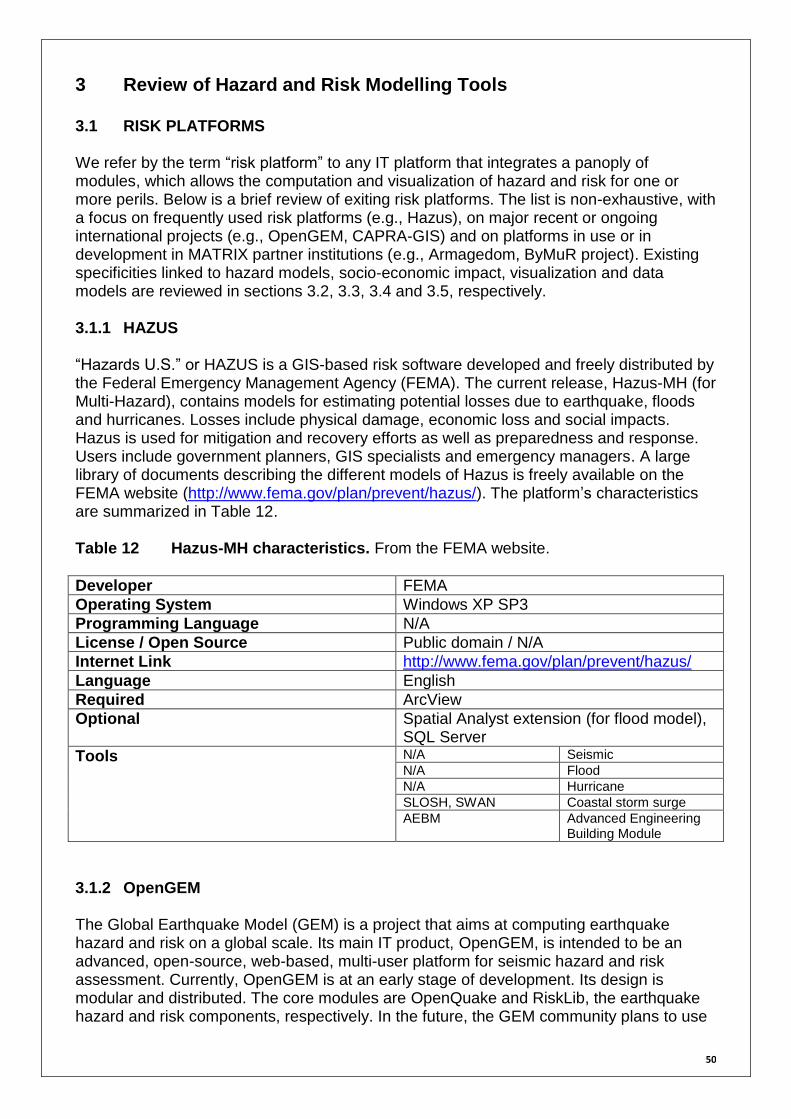
50

3 Review of Hazard and Risk Modelling Tools

3.1 RISK PLATFORMS We refer by the term “risk platform” to any IT platform that integrates a panoply of modules, which allows the computation and visualization of hazard and risk for one or more perils. Below is a brief review of exiting risk platforms. The list is non-exhaustive, with a focus on frequently used risk platforms (e.g., Hazus), on major recent or ongoing international projects (e.g., OpenGEM, CAPRA-GIS) and on platforms in use or in development in MATRIX partner institutions (e.g., Armagedom, ByMuR project). Existing specificities linked to hazard models, socio-economic impact, visualization and data models are reviewed in sections 3.2, 3.3, 3.4 and 3.5, respectively. 3.1.1 HAZUS “Hazards U.S.” or HAZUS is a GIS-based risk software developed and freely distributed by the Federal Emergency Management Agency (FEMA). The current release, Hazus-MH (for Multi-Hazard), contains models for estimating potential losses due to earthquake, floods and hurricanes. Losses include physical damage, economic loss and social impacts. Hazus is used for mitigation and recovery efforts as well as preparedness and response. Users include government planners, GIS specialists and emergency managers. A large library of documents describing the different models of Hazus is freely available on the FEMA website (http://www.fema.gov/plan/prevent/hazus/). The platform’s characteristics are summarized in Table 12. Table 12 Hazus-MH characteristics. From the FEMA website.

Developer FEMA

Operating System Windows XP SP3

Programming Language N/A

License / Open Source Public domain / N/A

Internet Link http://www.fema.gov/plan/prevent/hazus/

Language English

Required ArcView

Optional Spatial Analyst extension (for flood model), SQL Server

Tools N/A Seismic

N/A Flood

N/A Hurricane

SLOSH, SWAN Coastal storm surge

AEBM Advanced Engineering Building Module

3.1.2 OpenGEM The Global Earthquake Model (GEM) is a project that aims at computing earthquake hazard and risk on a global scale. Its main IT product, OpenGEM, is intended to be an advanced, open-source, web-based, multi-user platform for seismic hazard and risk assessment. Currently, OpenGEM is at an early stage of development. Its design is modular and distributed. The core modules are OpenQuake and RiskLib, the earthquake hazard and risk components, respectively. In the future, the GEM community plans to use

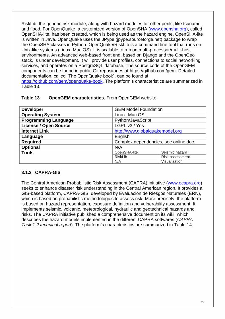
51

RiskLib, the generic risk module, along with hazard modules for other perils, like tsunami and flood. For OpenQuake, a customized version of OpenSHA (www.opensha.org), called OpenSHA-lite, has been created, which is being used as the hazard engine. OpenSHA-lite is written in Java. OpenQuake uses the JPype (jpype.sourceforge.net) package to wrap the OpenSHA classes in Python. OpenQuake/RiskLib is a command-line tool that runs on Unix-like systems (Linux, Mac OS). It is scalable to run on multi-processor/multi-host environments. An advanced web-based front end, based on Django and the OpenGeo stack, is under development. It will provide user profiles, connections to social networking services, and operates on a PostgreSQL database. The source code of the OpenGEM components can be found in public Git repositories at https://github.com/gem. Detailed documentation, called “The OpenQuake book”, can be found at https://github.com/gem/openquake-book. The platform’s characteristics are summarized in Table 13.

Table 13 OpenGEM characteristics. From OpenGEM website.

Developer GEM Model Foundation

Operating System Linux, Mac OS

Programming Language Python/JavaScript

License / Open Source LGPL v3 / Yes

Internet Link http://www.globalquakemodel.org

Language English

Required Complex dependencies, see online doc.

Optional N/A

Tools OpenSHA-lite Seismic hazard

RiskLib Risk assessment

N/A Visualization

3.1.3 CAPRA-GIS The Central American Probabilistic Risk Assessment (CAPRA) initiative (www.ecapra.org) seeks to enhance disaster risk understanding in the Central American region. It provides a GIS-based platform, CAPRA-GIS, developed by Evaluación de Riesgos Naturales (ERN), which is based on probabilistic methodologies to assess risk. More precisely, the platform is based on hazard representation, exposure definition and vulnerability assessment. It implements seismic, volcanic, meteorological, hydraulic and geotechnical hazards and risks. The CAPRA initiative published a comprehensive document on its wiki, which describes the hazard models implemented in the different CAPRA softwares (CAPRA Task 1.2 technical report). The platform’s characteristics are summarized in Table 14.

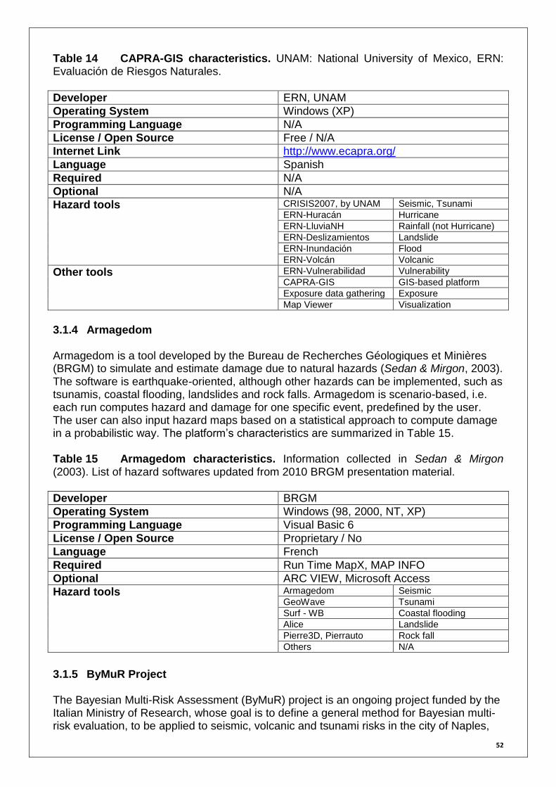
52

Table 14 CAPRA-GIS characteristics. UNAM: National University of Mexico, ERN: Evaluación de Riesgos Naturales.

Developer ERN, UNAM

Operating System Windows (XP)

Programming Language N/A

License / Open Source Free / N/A

Internet Link http://www.ecapra.org/

Language Spanish

Required N/A

Optional N/A

Hazard tools CRISIS2007, by UNAM Seismic, Tsunami

ERN-Huracán Hurricane

ERN-LluviaNH Rainfall (not Hurricane)

ERN-Deslizamientos Landslide

ERN-Inundación Flood

ERN-Volcán Volcanic

Other tools ERN-Vulnerabilidad Vulnerability

CAPRA-GIS GIS-based platform

Exposure data gathering Exposure

Map Viewer Visualization

3.1.4 Armagedom Armagedom is a tool developed by the Bureau de Recherches Géologiques et Minières (BRGM) to simulate and estimate damage due to natural hazards (Sedan & Mirgon, 2003). The software is earthquake-oriented, although other hazards can be implemented, such as tsunamis, coastal flooding, landslides and rock falls. Armagedom is scenario-based, i.e. each run computes hazard and damage for one specific event, predefined by the user. The user can also input hazard maps based on a statistical approach to compute damage in a probabilistic way. The platform’s characteristics are summarized in Table 15. Table 15 Armagedom characteristics. Information collected in Sedan & Mirgon (2003). List of hazard softwares updated from 2010 BRGM presentation material.

Developer BRGM

Operating System Windows (98, 2000, NT, XP)

Programming Language Visual Basic 6

License / Open Source Proprietary / No

Language French

Required Run Time MapX, MAP INFO

Optional ARC VIEW, Microsoft Access

Hazard tools Armagedom Seismic

GeoWave Tsunami

Surf - WB Coastal flooding

Alice Landslide

Pierre3D, Pierrauto Rock fall

Others N/A

3.1.5 ByMuR Project The Bayesian Multi-Risk Assessment (ByMuR) project is an ongoing project funded by the Italian Ministry of Research, whose goal is to define a general method for Bayesian multi-risk evaluation, to be applied to seismic, volcanic and tsunami risks in the city of Naples,

53

Italy (http://bymur.bo.ingv.it/). The main output of the ByMuR project is a software to analyze and compare risks in Naples. It is composed of three independent modules for seismic, volcanic and tsunami hazards, a vulnerability module for vulnerability assessment for all hazards and a risk module for risk calculation and comparison. All of these modules are coordinated by a main module consisting of a GUI (ByMuR, 2011). The platform’s characteristics are summarized in Table 16. Table 16 ByMuR software characteristics. From ByMuR (2011).

Developer INGV

Operating System Cross-platform

Programming Language Python

Data Protocols MySQL DB, XML for data exchange

License / Open Source Free / Yes

Internet Link http://bymur.bo.ingv.it/

Language English

Required N/A

Optional N/A

Hazard tools BET_VH modified Volcanic

No name in 07/2011 Seismic

No name in 07/2011 Tsunami

The ByMuR software is based on the existing tool BET_VH (Bayesian Event Tree for Volcanic Hazard, see Table 17), a probabilistic tool for long-term volcanic hazard assessment, which hasbeen completely re-designed within the framework of the multi-risk project. The BET_VH tool is described in detail by Marzocchi et al. (2010) (see also the BET_EF tool, BET for Eruption Forecasting, described by Marzocchi et al., 2009). The BET software tools are based on a model that provides probabilities of any specific event, by merging all the relevant available information such as theoretical models, a priori beliefs, or past data (see BET brief description in section 2.3.2 and BET development for multi-risk in the WP3 of the MATRIX project). A draft of the ByMuR software is expected for December 2011 (as indicated on http://bymur.bo.ingv.it/). Table 17 BET_VH tool characteristics. Information collected from the BET_EF 2.0 Manual, available at http://bet.bo.ingv.it/. INGV: Istituto Nazionale di Geofisica e Vulcanologia

Developer INGV

Operating System Windows

Programming Language Visual Basic

License / Open Source Free / No

Internet Link http://bet.bo.ingv.it/

Language English

Required .NET framework

Additional tools BET_UPGRADE, GUI

3.1.6 RiskScape Finally, a description should be made of the recently proposed RiskScape multi-risk platform, developed in the project Regional RiskScape by the Reseach Organizations GNS Science and the National Institute of Water and Atmospheric Research Ltd. (NIWA) in New Zealand (Schmidt et al., 2011). RiskScape results from the development of a

54

generic technology for modelling risks from different natural hazards and for various elements at risk. The generic framework of the software prototype is described in Schmidt et al. (2011), where earthquake, volcanic ash fall, flood, wind and tsunami risks are also modelled for test sites in New Zealand. RiskScape includes modules for hazards, assets, loss functions and aggregation units. Implementation of the whole system is based on three fundamental components: Module Specifications (i.e. data models in XML), Standard Types for module relationships (i.e. data exchange models in XML) and Functions for calculating risk (in Java). Schmidt et al. (2011) present a generic data model for the different modules of RiskScape as well as workflows to link the different modules. The RiskScape User Manual (RiskScape, 2010) is a precious source of information regarding the different attribute types defined for hazard and exposure data structures. This is discussed in detail in section 3.5. The platform’s characteristics are summarized in Table 18. Table 18 RiskScape characteristics. Information collected from Schmidt et al. (2011).

Developer GNS, NIWA

Operating System Cross-platform

Programming Language Java (functions), XML (data exchange)

License / Open Source Proprietary / No

Internet Link http://www.riskscape.org.nz

Language English

Required Java Virtual Machine

Optional Broadband internet

Additional Tools GUI, Web-GIS

3.2 HAZARD MODELS As indicated in section 1.2.1 “Platform modular structure overview”, the MATRIX multi-risk platform will not compute hazards but rather will call upon external hazard models (“hazard plug-ins”) or directly use pre-computed stochastic event sets. In both cases, a model must be available to provide hazard intensity surfaces to the main platform. Table 19 lists the hazards to be implemented in the MATRIX project. For each hazard, a review of existing models is made, with a focus on open source models (e.g., OpenSHA for seismic hazard) and other models developed by MATRIX partners (e.g., for meteorological and flood hazards).

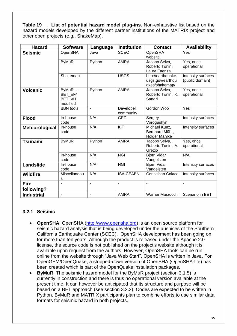
55

Table 19 List of potential hazard model plug-ins. Non-exhaustive list based on the hazard models developed by the different partner institutions of the MATRIX project and other open projects (e.g., ShakeMap).

Hazard Software Language Institution Contact Availability

Seismic OpenSHA Java SCEC OpenSHA website

Yes

ByMuR Python AMRA Jacopo Selva, Roberto Tonini, Laura Faenza

Yes, once operational

Shakemap - USGS http://earthquake.usgs.gov/earthquakes/shakemap/

Intensity surfaces (public domain)

Volcanic ByMuR – BET_EF/ BET_VH modified

Python AMRA Jacopo Selva, Roberto Tonini, K. Sandri

Yes, once operational

BBN tools - Developer community

Gordon Woo Yes

Flood In-house code

N/A GFZ Sergey Vorogushyn

Intensity surfaces

Meteorological In-house code

N/A KIT Michael Kunz, Bernhard Mühr, Holger Mahlke

Intensity surfaces

Tsunami ByMuR Python AMRA Jacopo Selva, Roberto Tonini, A. Grezio

Yes, once operational

In-house code

N/A NGI Bjorn Vidar Vangelsten

N/A

Landslide In-house code

N/A NGI Bjorn Vidar Vangelsten

Intensity surfaces

Wildfire Miscellaneous

N/A ISA-CEABN Conceicao Colaco Intensity surfaces

Fire following?

- - - - -

Industrial - - AMRA Warner Marzocchi Scenario in BET

3.2.1 Seismic

OpenSHA: OpenSHA (http://www.opensha.org) is an open source platform for seismic hazard analysis that is being developed under the auspices of the Southern California Earthquake Center (SCEC). OpenSHA development has been going on for more than ten years. Although the product is released under the Apache 2.0 license, the source code is not published on the project's website although it is available upon request from the authors. However, OpenSHA tools can be run online from the website through “Java Web Start”. OpenSHA is written in Java. For OpenGEM/OpenQuake, a stripped-down version of OpenSHA (OpenSHA-lite) has been created which is part of the OpenQuake installation packages.

ByMuR: The seismic hazard model for the ByMuR project (section 3.1.5) is currently in construction and there is thus no operational version available at the present time. It can however be anticipated that its structure and purpose will be based on a BET approach (see section 3.2.2). Codes are expected to be written in Python. ByMuR and MATRIX participants plan to combine efforts to use similar data formats for seismic hazard in both projects.

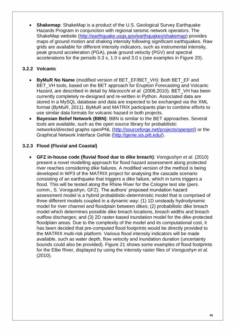
56

Shakemap: ShakeMap is a product of the U.S. Geological Survey Earthquake Hazards Program in conjunction with regional seismic network operators. The ShakeMap website (http://earthquake.usgs.gov/earthquakes/shakemap) provides maps of ground motion and shaking intensity following significant earthquakes. Raw grids are available for different intensity indicators, such as instrumental intensity, peak ground acceleration (PGA), peak ground velocity (PGV) and spectral accelerations for the periods 0.3 s, 1.0 s and 3.0 s (see examples in Figure 20).

3.2.2 Volcanic

ByMuR No Name (modified version of BET_EF/BET_VH): Both BET_EF and BET_VH tools, based on the BET approach for Eruption Forecasting and Volcanic Hazard, are described in detail by Marzocchi et al. (2008,2010). BET_VH has been currently completely re-designed and re-written in Python. Associated data are stored in a MySQL database and data are expected to be exchanged via the XML format (ByMuR, 2011). ByMuR and MATRIX participants plan to combine efforts to use similar data formats for volcanic hazard in both projects.

Bayesian Belief Network (BBN): BBN is similar to the BET approaches. Several tools are available, such as the open source library for probabilistic networks/directed graphs openPNL (http://sourceforge.net/projects/openpnl) or the Graphical Network Interface GeNIe (http://genie.sis.pitt.edu/).

3.2.3 Flood (Fluvial and Coastal)

GFZ in-house code (fluvial flood due to dike breach): Vorogushyn et al. (2010) present a novel modelling approach for flood hazard assessment along protected river reaches considering dike failures. A modified version of the method is being developed in WP3 of the MATRIX project for analysing the cascade scenario consisting of an earthquake that triggers a dike failure, which in turns triggers a flood. This will be tested along the Rhine River for the Cologne test site (pers. comm., S. Vorogushyn, GFZ). The authors’ proposed inundation hazard assessment model is a hybrid probabilistic-deterministic model that is comprised of three different models coupled in a dynamic way: (1) 1D unsteady hydrodynamic model for river channel and floodplain between dikes; (2) probabilistic dike breach model which determines possible dike breach locations, breach widths and breach outflow discharges; and (3) 2D raster-based inundation model for the dike-protected floodplain areas. Due to the complexity of the model and its computational cost, it has been decided that pre-computed flood footprints would be directly provided to the MATRIX multi-risk platform. Various flood intensity indicators will be made available, such as water depth, flow velocity and inundation duration (uncertainty bounds could also be provided). Figure 21 shows some examples of flood footprints for the Elbe River, displayed by using the intensity raster files of Vorogushyn et al. (2010).

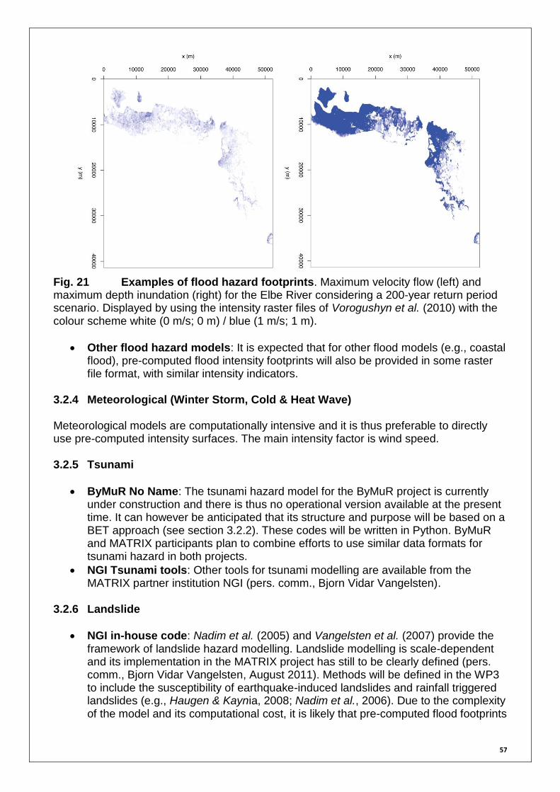
57

Fig. 21 Examples of flood hazard footprints. Maximum velocity flow (left) and maximum depth inundation (right) for the Elbe River considering a 200-year return period scenario. Displayed by using the intensity raster files of Vorogushyn et al. (2010) with the colour scheme white (0 m/s; 0 m) / blue (1 m/s; 1 m).

Other flood hazard models: It is expected that for other flood models (e.g., coastal flood), pre-computed flood intensity footprints will also be provided in some raster file format, with similar intensity indicators.

3.2.4 Meteorological (Winter Storm, Cold & Heat Wave) Meteorological models are computationally intensive and it is thus preferable to directly use pre-computed intensity surfaces. The main intensity factor is wind speed. 3.2.5 Tsunami

ByMuR No Name: The tsunami hazard model for the ByMuR project is currently under construction and there is thus no operational version available at the present time. It can however be anticipated that its structure and purpose will be based on a BET approach (see section 3.2.2). These codes will be written in Python. ByMuR and MATRIX participants plan to combine efforts to use similar data formats for tsunami hazard in both projects.

NGI Tsunami tools: Other tools for tsunami modelling are available from the MATRIX partner institution NGI (pers. comm., Bjorn Vidar Vangelsten).

3.2.6 Landslide

NGI in-house code: Nadim et al. (2005) and Vangelsten et al. (2007) provide the framework of landslide hazard modelling. Landslide modelling is scale-dependent and its implementation in the MATRIX project has still to be clearly defined (pers. comm., Bjorn Vidar Vangelsten, August 2011). Methods will be defined in the WP3 to include the susceptibility of earthquake-induced landslides and rainfall triggered landslides (e.g., Haugen & Kaynia, 2008; Nadim et al., 2006). Due to the complexity of the model and its computational cost, it is likely that pre-computed flood footprints

58

will be directly provided to the MATRIX multi-risk platform. A large number of landslide intensity indicators are available, including maximum velocity (Fig. 22).

Fig. 22 Example of landslide hazard footprint. Modelled maximum velocity (in m/s) of an avalanche at Ryggfonn, Stryn, Western Norway. Courtesy of Peter Gauer, NGI. 3.2.7 Wildfire ISA-CEABN does not have any specific software to compute wildfire hazard and uses the same standard models as those produced by the U.S. Forest Services to estimate fire spread and intensity. These programs include some general predictions of maximum spotting distance that could be used in the platform. ISA-CEABN will provide footprints including fire intensity and trajectories, the result of expertise gained from the previous projects SALTUS, FIRE PARADOX and TRANZFOR (pers. comm., Conceicao Colaco, August 2011). 3.2.8 Fire Following an Event At the present time, there is no Fire Following model available as a plug-in for the MATRIX platform. Although this hazard is not specified in the MATRIX Description of Work document, some examples, such as fire following earthquake, are well recognized as a hazard interaction that can lead to great losses. A comprehensive multi-risk platform must therefore include this hazard. 3.2.9 Industrial It is possible that specific industrial incident scenarios will be defined in the MATRIX project and implemented using a BET approach (e.g. Marzocchi et al., 2009). BETs can be

59

directly provided to the MATRIX platform, which translates them into event tables used as input in sampling procedures. 3.3 SOCIO-ECONOMIC IMPACT The social and economic impacts of multi-hazard and multi-risk are analysed in WP6 of the MATRIX project, which focuses on decision support for preparedness, response and mitigation strategies. While not represented on the diagram showing the different modules of the MATRIX multi-risk platform (Figure 1), a socioeconomic (or “indirect loss”) module could be added on top of the proposed (“direct”) loss module. This section reviews the socio-economic tools available from the MATRIX partners (DRNEP from UBC, section 3.3.1 and CATSIM from IIASA, section 3.3.2) as well as from the GEM project (SEIM, section 3.3.3). 3.3.1 Disaster Response Network Enabled Platform The Disaster Response Network Enabled Platform (DR NEP) is a distributed system that integrates a set of independently developed infrastructure and disaster simulators. Its goal is to assist first responders to a disaster in the preparation, response and recovery phases. The DR NEP is developed by the University of British Columbia (UBC), with input from the University of Western Ontario on disaster planning strategies and from the University of New Brunswick on human decision making strategies (http://drnep.ece.ubc.ca/index.html). It uses a master-slave pattern, with one master simulator orchestrating all of the others, based on a central system clock (Gonzaléz et al., 2011). The master simulator, Interdependent Simulator (I2Sim), developed by UBC, is a custom software suite that allows the modelling of interactions between distinct infrastructures, utilities, business processes and emergency operations. Other simulators include: BRAHMS, PSSe, EPANET and MicroTran (not considered in the MATRIX project). The DR NEP enables linkage between various simulators from different organizations, which use different modelling approaches and different data models. The DR NEP approach is based on system theory to develop a common data model and efficient communication schemes. The approach could for example be used to create an interface with the MATRIX platform (pers. comm., Paul Lusina). The DR NEP hub is made up of a system bus, database and a multi-core server for communication and computation. The I2Sim platform’s characteristics are summarized in Table 20. Table 20 I2Sim characteristics. Information from UBC (2009).

Developer UBC

Operating System Windows

Programming Language Matlab

License / Open Source N/A

Internet Link http://www.i2sim.ca

Language English

Required N/A

Optional N/A

Additional Tools GUI, Visualization, I/O management (HRT)

60

3.3.2 CATastrophe SIMulator The CATastrophe SIMulation (CATSIM) model is a framework developed by the International Institute for Applied Systems Analysis (IIASA) to assess risk, economic resilience and fiscal vulnerability to extreme events. This tool can assist policy makers from governments, insurance companies, capital markets or disaster funds, in developing financing strategies for disaster risk. The models show the respective costs and consequences of financing alternatives on important indicators, e.g., economic growth or debt. CATSIM is composed of two modules and is equipped with a GIS. The first module is defined for risk assessment (loss estimation) with inputs being hazard, vulnerability and exposure. The second module shows the costs and benefits of different strategies to manage risk. CATSIM includes also a stochastic mode to calculate an optimal mix of ex-ante and ex-post measures by solving a multistage stochastic optimization problem (ex-post and ex-ante being respectively the realised and predicted tracking errors that compare the financial model to the portfolio). Figure 23 depicts the CATSIM framework. For more details, the reader should refer to the CATSIM webpage (http://www.iiasa.ac.at/ Research/RAV/Projects/catsim.html), Mechler et al. (2010) and Hochrainer et al. (2011). The socio-economic platform’s characteristics are summarized in Table 21.

Fig. 23 CATSIM framework. Assessment of fiscal vulnerability and management of extreme event risk. Courtesy of IIASA.

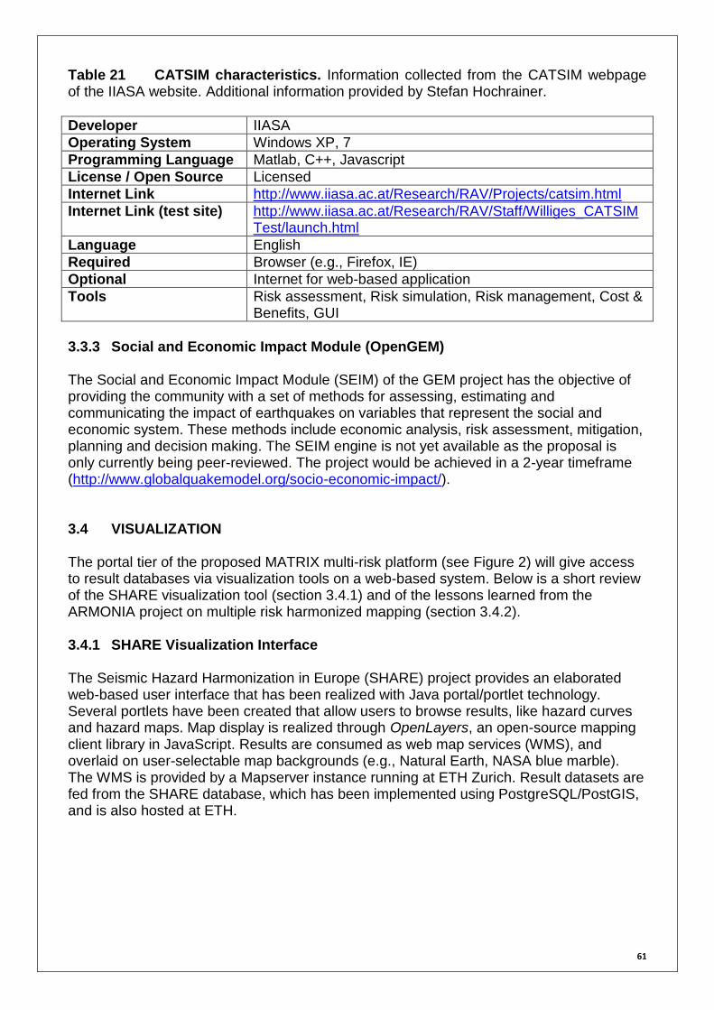
61

Table 21 CATSIM characteristics. Information collected from the CATSIM webpage of the IIASA website. Additional information provided by Stefan Hochrainer.

Developer IIASA

Operating System Windows XP, 7

Programming Language Matlab, C++, Javascript

License / Open Source Licensed

Internet Link http://www.iiasa.ac.at/Research/RAV/Projects/catsim.html

Internet Link (test site) http://www.iiasa.ac.at/Research/RAV/Staff/Williges_CATSIMTest/launch.html

Language English

Required Browser (e.g., Firefox, IE)

Optional Internet for web-based application

Tools Risk assessment, Risk simulation, Risk management, Cost & Benefits, GUI

3.3.3 Social and Economic Impact Module (OpenGEM) The Social and Economic Impact Module (SEIM) of the GEM project has the objective of providing the community with a set of methods for assessing, estimating and communicating the impact of earthquakes on variables that represent the social and economic system. These methods include economic analysis, risk assessment, mitigation, planning and decision making. The SEIM engine is not yet available as the proposal is only currently being peer-reviewed. The project would be achieved in a 2-year timeframe (http://www.globalquakemodel.org/socio-economic-impact/). 3.4 VISUALIZATION The portal tier of the proposed MATRIX multi-risk platform (see Figure 2) will give access to result databases via visualization tools on a web-based system. Below is a short review of the SHARE visualization tool (section 3.4.1) and of the lessons learned from the ARMONIA project on multiple risk harmonized mapping (section 3.4.2). 3.4.1 SHARE Visualization Interface The Seismic Hazard Harmonization in Europe (SHARE) project provides an elaborated web-based user interface that has been realized with Java portal/portlet technology. Several portlets have been created that allow users to browse results, like hazard curves and hazard maps. Map display is realized through OpenLayers, an open-source mapping client library in JavaScript. Results are consumed as web map services (WMS), and overlaid on user-selectable map backgrounds (e.g., Natural Earth, NASA blue marble). The WMS is provided by a Mapserver instance running at ETH Zurich. Result datasets are fed from the SHARE database, which has been implemented using PostgreSQL/PostGIS, and is also hosted at ETH.

62

Fig. 24 Example screenshot of the SHARE portal page. Showing the hazard map view. 3.4.2 OneGeology OneGeology (http://onegeology.org) is an initiative that aims at producing a collection of geological map data on a global scale. It provides an elaborate web interface (http://portal.onegeology.org) that allows an interactive map view of a base map with overlays of geological maps of several kinds. The map frontend is realized using the open-source JavaScript library OpenLayers. The user-provided data are accessed through standardized geospatial web services (WMS, WFS). WFS feeds can be encoded in GeoSciML (http://www.geosciml.org), a GML application schema for geosciences (see section 3.5.3). OpenGeology operates a registry of user-provided WMS and WFS services. Web services listed in the registry are identified through a set of standardized (ISO19115) metadata that has to be provided by the user. The registry is operated through an instance of the GeoNetwork opensource. 3.4.3 Lessons Learned from the ARMONIA Project The work done in the ARMONIA project on applied multi-risk mapping of natural hazards for impact assessment (from the 6th Framework Programme of European Commission) is reviewed in Task 5.1 (WP5) of the MATRIX project. Below are thus only presented the main bullet points to take from ARMONIA (ARMONIA, 2007) being considered in the mapping procedures being developed for the MATRIX multi-risk platform:

Common metrics for multi-risk mapping: Use a same metric for different hazards such as a common intensity scale index (e.g., low, medium, high), damage (e.g., % of cracks in walls, % of unsafe buildings, % of collapsed buildings) or economic loss.

Spatiotemporal scale clearly defined: Any methodological approach is strictly dependent on the scale of analysis and representation (local, regional, national

63

scale). Moreover, values of likely damage/risk should be summarized in terms of vulnerability curves for the same return periods (e.g., 1% or 0.1%). The choice depends on the purpose of the end-user.

Mapping information via colour scales: Mapping hazard and risk must be done in a way which is as informative as possible, without biasing decision-makers’ perceptions (e.g., the colour red has been identified as being strongly affective). WP3 of the ARMONIA project suggested that a two-parametric colour range could be used for the production of maps to indicate, through variations of colour and hue, both monetary and non-monetary risk. The colour scheme must be based on colours that are perceived relatively neutral (e.g., blue and orange, Figure 24).

Fig. 25 Colour scale proposed by ARMONIA project for mapping risk. Redrawn from Figure 5.3 of ARMONIA (2007). 3.5 DATA MODELS Hazard and risk homogenization is required in any multi-risk framework. Different methods exist such as NRML (section 3.5.1) and GeoSciML (section 3.5.2). Some generic frameworks are also available (section 3.5.3). 3.5.1 NRML (OpenGEM) The data model for earthquake hazard and risk that is being used in OpenQuake/OpenGEM has been formulated as an XML Schema. XML instance documents conforming to that schema are used for the exchange of data products created by the engine with collaborators, and also for communication between components of OpenGEM. The XML dialect that has been developed is called NRML, the Natural Hazards' Risk Markup Language (Euchner et al., 2011). The schema has a modular design and is split up into several sub-schemas for hazard, risk, logic tree, seismic

64

sources, and general data types. Furthermore, it is an application schema of GML (Geographic Markup Language), which is an OGC standard for the description of geospatial features. The seismic hazard part covers seismic source parameters and rupture geometries, hazard curves and ground motion fields. The seismic risk part contains loss and loss ratio curves, exposure portfolios, and vulnerability curves. NRML leverages existing standards, such as the GML, and QuakeML (http://www.quakeml.org), a data model for seismology. 3.5.2 GeoSciML Geospatial data to be delivered through OneGeology (section 3.4.2) can be based on the GeoSciML data model. GeoSciML provides an extensive vocabulary for the geosciences that can be browsed online at http://srvgeosciml.brgm.fr/eXist2010/brgm/client.html. A standard-conforming representation of the vocabulary (RDF, OWL, SKOS) is available through web services from BRGM. 3.5.3 RiskScape RiskScape provides a generic framework for risk modeling (see section 3.1.6). It is a generic tool in a sense that risk analyses can be performed for different hazard scenarios, exposures, and vulnerabilities, as long as the relevant input data is fed to the program in the required input formats. This is the same concept as the one envisioned for the MATRIX platform, with the difference that in MATRIX the hazard interdependencies and the time-dependency of the vulnerability are accounted for. What makes RiskScape particularly interesting is that within the project a vocabulary has been defined (Table 22), which is partly based on the terminology of the United Nations' International Strategy for Disaster Reduction (UNISDR, 2009). This vocabulary can be used as a starting point for the data model to be developed for MATRIX.

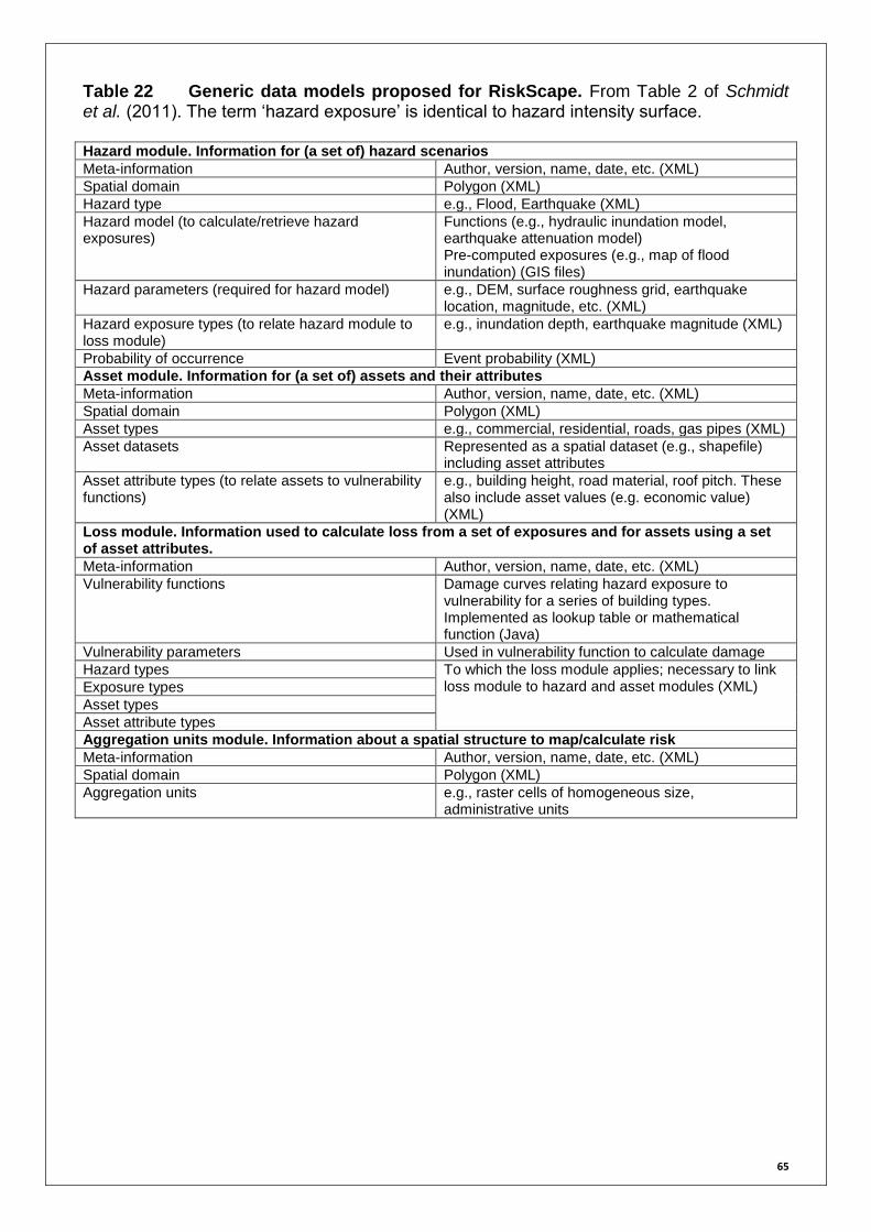
65

Table 22 Generic data models proposed for RiskScape. From Table 2 of Schmidt et al. (2011). The term ‘hazard exposure’ is identical to hazard intensity surface. Hazard module. Information for (a set of) hazard scenarios

Meta-information Author, version, name, date, etc. (XML)

Spatial domain Polygon (XML)

Hazard type e.g., Flood, Earthquake (XML)

Hazard model (to calculate/retrieve hazard exposures)

Functions (e.g., hydraulic inundation model, earthquake attenuation model) Pre-computed exposures (e.g., map of flood inundation) (GIS files)

Hazard parameters (required for hazard model) e.g., DEM, surface roughness grid, earthquake location, magnitude, etc. (XML)

Hazard exposure types (to relate hazard module to loss module)

e.g., inundation depth, earthquake magnitude (XML)

Probability of occurrence Event probability (XML)

Asset module. Information for (a set of) assets and their attributes

Meta-information Author, version, name, date, etc. (XML)

Spatial domain Polygon (XML)

Asset types e.g., commercial, residential, roads, gas pipes (XML)

Asset datasets Represented as a spatial dataset (e.g., shapefile) including asset attributes

Asset attribute types (to relate assets to vulnerability functions)

e.g., building height, road material, roof pitch. These also include asset values (e.g. economic value) (XML)

Loss module. Information used to calculate loss from a set of exposures and for assets using a set of asset attributes.

Meta-information Author, version, name, date, etc. (XML)

Vulnerability functions Damage curves relating hazard exposure to vulnerability for a series of building types. Implemented as lookup table or mathematical function (Java)

Vulnerability parameters Used in vulnerability function to calculate damage

Hazard types To which the loss module applies; necessary to link loss module to hazard and asset modules (XML) Exposure types

Asset types

Asset attribute types

Aggregation units module. Information about a spatial structure to map/calculate risk

Meta-information Author, version, name, date, etc. (XML)

Spatial domain Polygon (XML)

Aggregation units e.g., raster cells of homogeneous size, administrative units

66

4 Build v. 1.x (MATRIX Common IT Platform): IT Architecture Development 4.1 PREREQUISITES From several suggestions made by participants to coin the official name of the MATRIX IT platform, the Project Management Team picked the name MATRIX-CITY (MATRIX Common IT sYstem). The review of existing platforms in the previous section was conducted to determine if one of the existing platforms could be used as a basis for the development of the MATRIX platform. No other framework seems to be suitable to be directly forked, but OpenQuake uses modern technologies that will also be used for MATRIX-CITY (Python programming language, XML data interchange format, AMPQ-based task distribution, distributed KVS store, PostgreSQL/PostGIS geospatial database). As a further advantage, part of the OpenQuake development team is based at ETH Zurich, which makes it easier to exchange expertise between the development teams. 4.1.1 IT Resource Allocation At the present stage, it is not fully clear how high the platform's demands for computational power will be. However, since no hazard computations are performed, and already pre-computed intensity surfaces will be used, we assume that no dedicated high-performance computing infrastructure will be needed. ETH will provide a server with 48 cores, based on AMD 12-core processors, and a large shared memory of 128 GB RAM for computations with the platform. This architecture should be sufficiently flexible to accommodate the computational needs regarding memory consumption per process, and also regarding the parallelization of computational tasks. 4.1.2 Other prerequisites There are several standards that regulate the presentation of results from projects in the geospatial domain (INSPIRE directive). In particular, it is demanded that map layer data is published through standardized web services. These are Web Map Service (WMS) and Web Feature Service (WFS), as defined in the OGC standard documentation. We will adhere to these standards. The results will be served through a well-established GIS infrastructure based on a PostgreSQL/PostGIS database and OSGeo MapServer middleware, and they will be consumed client-side via the OpenLayers library. 4.2 ASPECTS OF SOFTWARE ENGINEERING 4.2.1 Development Approach The MATRIX-CITY will be developed using an end-to-end, “fail-fast” strategy. This means that development will be top-down, with early prototyping of components that do not necessarily fulfill all requirements in the first pass (“stubs”). Once such a skeleton has been created, the individual modules will be fleshed out regarding correctness and completeness. To aid in this process, we will make use of test-driven development, meaning that the correct execution of small code fragments is ensured by corresponding test routines that are run automatically (unit tests). In addition to these fine-grained functionality tests, there will be automated tests that check for the integrity and correct

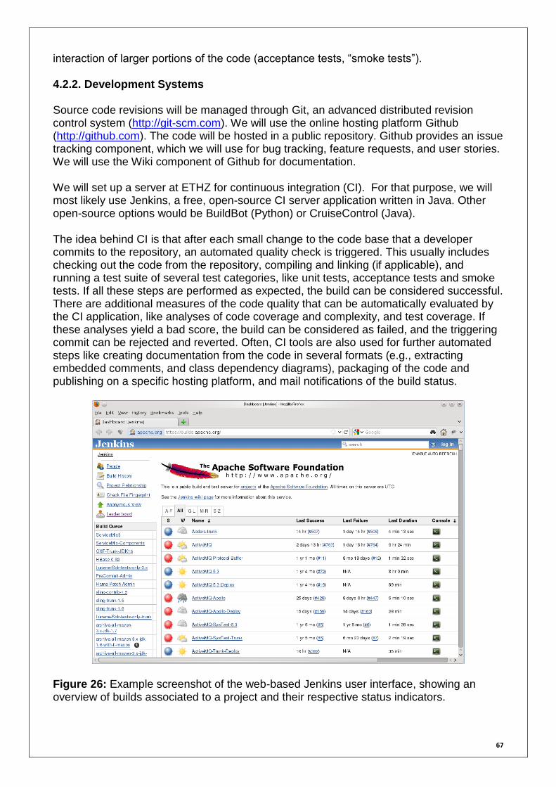
67

interaction of larger portions of the code (acceptance tests, “smoke tests”). 4.2.2. Development Systems Source code revisions will be managed through Git, an advanced distributed revision control system (http://git-scm.com). We will use the online hosting platform Github (http://github.com). The code will be hosted in a public repository. Github provides an issue tracking component, which we will use for bug tracking, feature requests, and user stories. We will use the Wiki component of Github for documentation. We will set up a server at ETHZ for continuous integration (CI). For that purpose, we will most likely use Jenkins, a free, open-source CI server application written in Java. Other open-source options would be BuildBot (Python) or CruiseControl (Java). The idea behind CI is that after each small change to the code base that a developer commits to the repository, an automated quality check is triggered. This usually includes checking out the code from the repository, compiling and linking (if applicable), and running a test suite of several test categories, like unit tests, acceptance tests and smoke tests. If all these steps are performed as expected, the build can be considered successful. There are additional measures of the code quality that can be automatically evaluated by the CI application, like analyses of code coverage and complexity, and test coverage. If these analyses yield a bad score, the build can be considered as failed, and the triggering commit can be rejected and reverted. Often, CI tools are also used for further automated steps like creating documentation from the code in several formats (e.g., extracting embedded comments, and class dependency diagrams), packaging of the code and publishing on a specific hosting platform, and mail notifications of the build status.

Figure 26: Example screenshot of the web-based Jenkins user interface, showing an overview of builds associated to a project and their respective status indicators.

68

4.2.3 Programming and Data Exchange Languages Python will be used as the main programming language. Python is a modern, interpreted, fully object-oriented open source programming language that is well suited for rapid prototyping. It is becoming increasingly popular recently in scientific as well as in business/enterprise contexts, as it is also evidenced by the fact that two of the risk frameworks reviewed in Section 3 use Python as their main programming language (OpenQuake, ByMuR). Python provides support for many aspects of up-to-date programming technologies, e.g., database access (SQL and NoSQL), message-queue based processing, XML parsing and validation, GIS applications, authentication/authorisation and encryption, web services and web client programming. Test-driven development is supported through several Python packages. Code fragments in other languages (C/C++, Fortran, Java, R) can also easily be embedded and integrated in Python code through add-on libraries. We will create a UML (Unified Modelling Language) representation of the data model for hazard and risk. For that purpose, the graphical UML tool Enterprise Architect from Sparxsystems will be used. The UML model will then serve as the basis for other representations, like XML and SQL schemas. For data exchange, we will create an XML-based serialization format of the data model. This will be an extension of the already existing NRML format (Natural hazards' Risk Markup Language) that has been developed in the course of the OpenGEM project. In some cases, Shapefiles will be used as the data exchange format for geospatial data sets. For extensive raster-type geospatial datasets, a well-established raster format like GeoTIFF seems most suitable. For data sets without complex structure, like result matrices and vectors, or configuration files, a simple, plain-ASCII representation will suffice. The R codes developed for the platform sketch (Build 0.x) described in Section 2 will be ported to Python, using standard library packages numpy and scipy. In cases where this turns out to be problematic, R code can be run directly from Python using the package RPy. 4.2.4 Data Model MATRIX-CITY will be based on a data model for hazard and risk (Fig. 27). This data model will be created as a UML class diagram. We will use the existing NRML data model from OpenQuake, which exists as an XML Schema, as the basis. However, NRML so far only describes seismic hazard. We will add components to account for the other perils that are relevant for the virtual city (volcanic eruptions, floods, landslides). In the risk part, the asset and vulnerability modules will have to be expanded and harmonized. We will evaluate existing vocabularies in order to identify existing useful concepts (GeoSciML, RiskScape). We will also create other representations of the data model. One will be XML Schema, since we will use XML-encoded data as the interchange format. Furthermore, we will create an SQL database schema, and a Python representation of the UML class diagram.

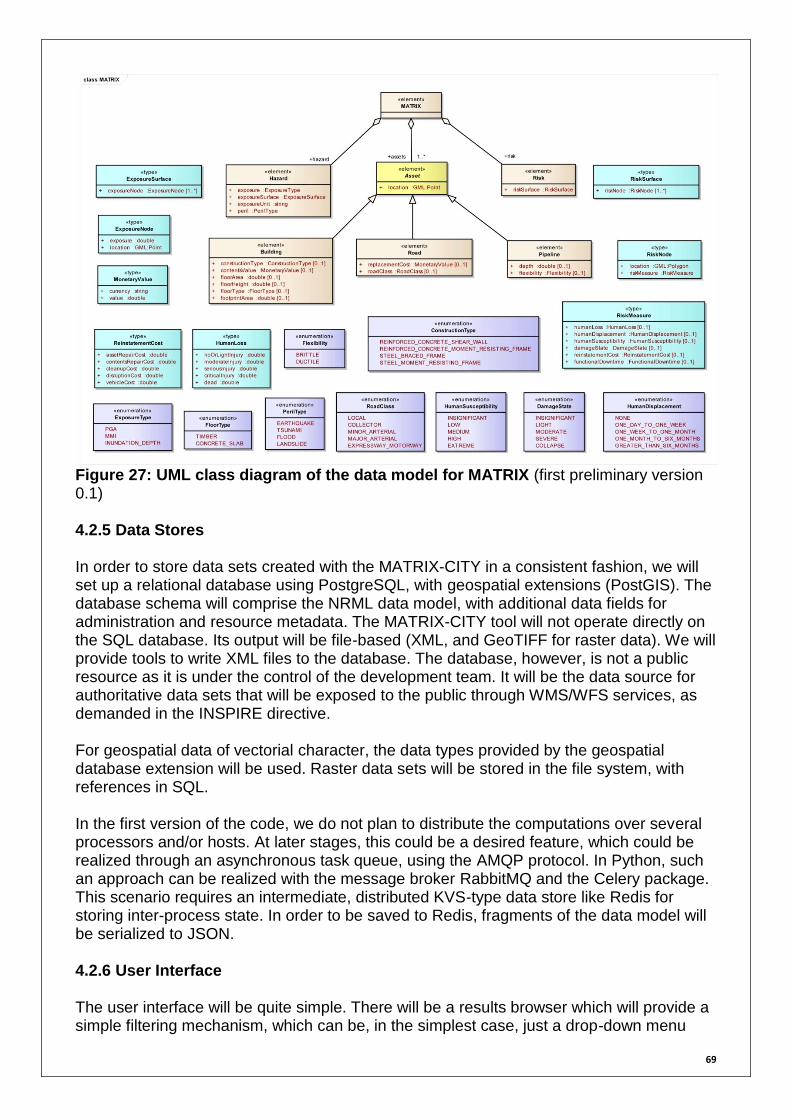
69

Figure 27: UML class diagram of the data model for MATRIX (first preliminary version 0.1) 4.2.5 Data Stores In order to store data sets created with the MATRIX-CITY in a consistent fashion, we will set up a relational database using PostgreSQL, with geospatial extensions (PostGIS). The database schema will comprise the NRML data model, with additional data fields for administration and resource metadata. The MATRIX-CITY tool will not operate directly on the SQL database. Its output will be file-based (XML, and GeoTIFF for raster data). We will provide tools to write XML files to the database. The database, however, is not a public resource as it is under the control of the development team. It will be the data source for authoritative data sets that will be exposed to the public through WMS/WFS services, as demanded in the INSPIRE directive. For geospatial data of vectorial character, the data types provided by the geospatial database extension will be used. Raster data sets will be stored in the file system, with references in SQL. In the first version of the code, we do not plan to distribute the computations over several processors and/or hosts. At later stages, this could be a desired feature, which could be realized through an asynchronous task queue, using the AMQP protocol. In Python, such an approach can be realized with the message broker RabbitMQ and the Celery package. This scenario requires an intermediate, distributed KVS-type data store like Redis for storing inter-process state. In order to be saved to Redis, fragments of the data model will be serialized to JSON. 4.2.6 User Interface The user interface will be quite simple. There will be a results browser which will provide a simple filtering mechanism, which can be, in the simplest case, just a drop-down menu

70

that allows one to select an item from a list. A slightly more elaborated version could allow making a selection based on simple resource metadata fields, like author name, time of creation, or spatial region. The results will be presented as maps (either static, or using a simple, Mapserver-powered OpenLayers window), and hyperlinks that refer to result datasets. Since result datasets for real scenarios might be confidential, the results page will be password-protected, and access rights will have to be granted by the consortium. 4.2.7 Testing Testing is essential to ensure that the code performs the desired tasks correctly. We will follow the test-driven development paradigm, trying to provide a high level of unit test coverage. Creating meaningful software tests is a non-trivial task, which requires close collaboration between scientists (as “product owners”) and programmers. Test-driven development is based on the concept that every small unit of code has a corresponding piece of code that checks whether the functionality intended by the programmer is provided correctly. Such a piece of test code can yield two results: either failure or success. Typically, in a test suite several hundreds or even thousands of such unit tests are collected. Upon running the test suite, all those tests are executed, and the results can give the programmer valuable insight whether the program works as intended, or, if tests are failing, on the nature of possible problems. Especially in later development stages this approach is useful, since new code often introduces side effects that break existing functionality. A carefully designed test suite can help to detect such failures through side effects that often go unnoticed, as early as possible. In the purest approach, test-driven development demands that the unit test code be written before the code that provides the intended functionality. Consequently, after this first step, the test suite will fail, because there is no code to be validated. In a subsequent step, the new code is written and improved, until its associated unit test passes. 4.2.8 License The system will be released under an open source license. In order to ensure that the codes written for the project stay free, it seems plausible to use the classical, strong-copyleft GNU General Public License (GPL version 3). This requires that all derived works will have to be released under GPL, too. Note that the copyright owners are always free to distribute copies of the code under a different license. This may be useful if commercial companies wish to use the code in proprietary, closed-source products. In this case, a re-licensed copy could be provided, either at no charge, or for an adequate financial compensation, if that seems appropriate. 4.3 DATA STRUCTURES

In Section 4.2.4, we have shown the UML class diagram for our first, preliminary version of the data model (v. 0.1). The data model is split into three main parts: Hazard, Assets, and Risk. Assets is realized as an abstract base class, from which concrete sub-classes for the different asset types under investigation are derived. In the class diagram, sub-classes for Buildings, Roads, and Pipelines are shown. This set will be expanded later. Both Hazard and Risk structures will be realized as GML feature sets. The features have both geospatial and non-geospatial attributes. For Hazard, the geospatial structure is of Point

71

type. This can be used to model nodes of a regular grid, but also irregular point sets can be described. In the Risk element, a Polygon model has been used, in order to describe area-type aggregation structures, like zones separated by administrative boundaries. The non-geospatial attributes in Hazard and Risk are used to describe the exposure intensity, which is a single floating-point number (hazard), and various risk measures that are modelled in the RiskMeasure data type (risk). The present description is strongly influenced by the RiskScape model, but in the future this will be strongly expanded, taking into account other existing data models and vocabularies.

72

5 Conclusions This report provides the multi-hazard and multi-risk frameworks to be implemented in the MATRIX platform as well as the IT strategies to be applied. Software development will be based on all guidelines, techniques, workflows and blueprints described in the report. The MATRIX platform is expected to be fully functional month 24. This means that members of the consortium would have provided sufficient data and background information to allow “experiments” to be carried out for the test cases. It will then be made available for members of the consortium for basic testing. A software manual and some Virtual City examples will be provided in the next report (D7.2).

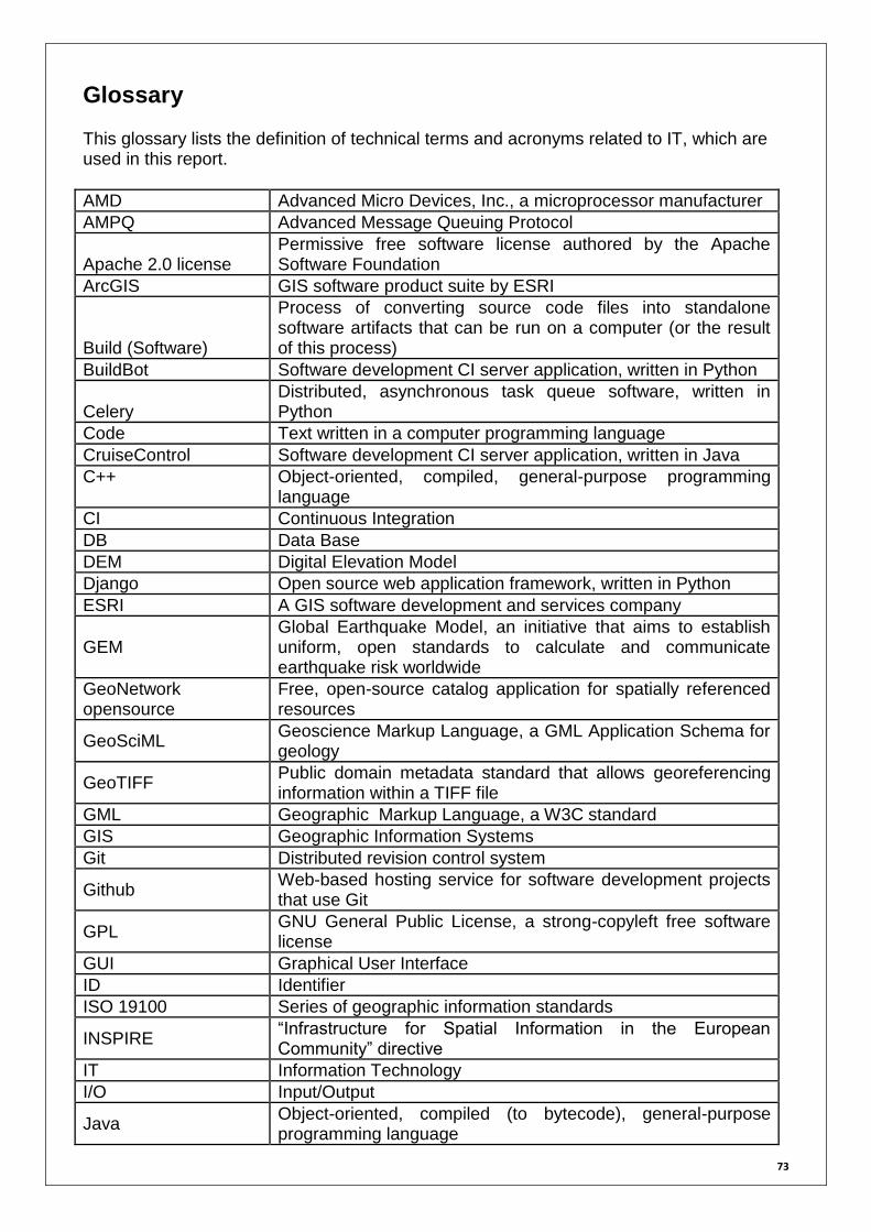
73

Glossary This glossary lists the definition of technical terms and acronyms related to IT, which are used in this report.

AMD Advanced Micro Devices, Inc., a microprocessor manufacturer

AMPQ Advanced Message Queuing Protocol

Apache 2.0 license Permissive free software license authored by the Apache Software Foundation

ArcGIS GIS software product suite by ESRI

Build (Software)

Process of converting source code files into standalone software artifacts that can be run on a computer (or the result of this process)

BuildBot Software development CI server application, written in Python

Celery Distributed, asynchronous task queue software, written in Python

Code Text written in a computer programming language

CruiseControl Software development CI server application, written in Java

C++ Object-oriented, compiled, general-purpose programming language

CI Continuous Integration

DB Data Base

DEM Digital Elevation Model

Django Open source web application framework, written in Python

ESRI A GIS software development and services company

GEM Global Earthquake Model, an initiative that aims to establish uniform, open standards to calculate and communicate earthquake risk worldwide

GeoNetwork opensource

Free, open-source catalog application for spatially referenced resources

GeoSciML Geoscience Markup Language, a GML Application Schema for geology

GeoTIFF Public domain metadata standard that allows georeferencing information within a TIFF file

GML Geographic Markup Language, a W3C standard

GIS Geographic Information Systems

Git Distributed revision control system

Github Web-based hosting service for software development projects that use Git

GPL GNU General Public License, a strong-copyleft free software license

GUI Graphical User Interface

ID Identifier

ISO 19100 Series of geographic information standards

INSPIRE “Infrastructure for Spatial Information in the European Community” directive

IT Information Technology

I/O Input/Output

Java Object-oriented, compiled (to bytecode), general-purpose programming language

74

Java Portal/Portlet Web site using components that adhere to the Java Portlet Specification (JSR168, JSR286)

JavaScript Prototype-based, dynamic scripting language

Java Web Start Framework that allows users to start application software for the Java Platform directly from the Internet

Jenkins Software development CI server application, written in Java

JPype Library that allows Python programs full access to Java class libraries

JSON JavaScript Object Notation, a lightweight text-based standard for data interchange

KVS Key-value store

LGPL GNU Lesser General Public License, a weak-copyleft free software license

Linux Computer operating system based on free and open source software, originally created by Linus Torvalds

MapServer Open source development environment for building spatially-enabled internet applications

MATLAB A numerical computing environment and programming language developed by MathWorks

MySQL RDBMS by MySQL AB (owned by Oracle Corporation)

Numpy Python package for numerical processing and scientific applications

NRML Natural hazards' Risk Markup Language

NoSQL “Not Only SQL”, database management systems that differ from classic RDBMS

OGC Open Geospatial Consortium

OMG Object Modeling Group

OpenGEM Web-based platform for earthquake hazard and risk computations by GEM, under development

OpenGeo Company that provides services for its open-source web mapping platform, also named OpenGeo

OpenQuake Open-source software engine driving OpenGEM

OpenLayers Open-source JavaScript library for displaying map data in web browsers

OpenSHA Open-source, Java-based platform for Seismic Hazard Analysis

OSGeo

Open Source Geospatial Foundation, a non-profit non-governmental organization that aims at supporting and promoting the collaborative development of open geospatial technologies and data

OWL Web Ontology Language, a family of knowledge representation languages for authoring ontologies

PDF Portable Document Format or Probability density function

Plug-In Software component that adds specific abilities to a larger software application

Portal Web site that functions as a point of access to information on the World Wide Web

PostgreSQL Free, open-source object-relational database management system

PostGIS Add-on for PostgreSQL that adds support for geographic

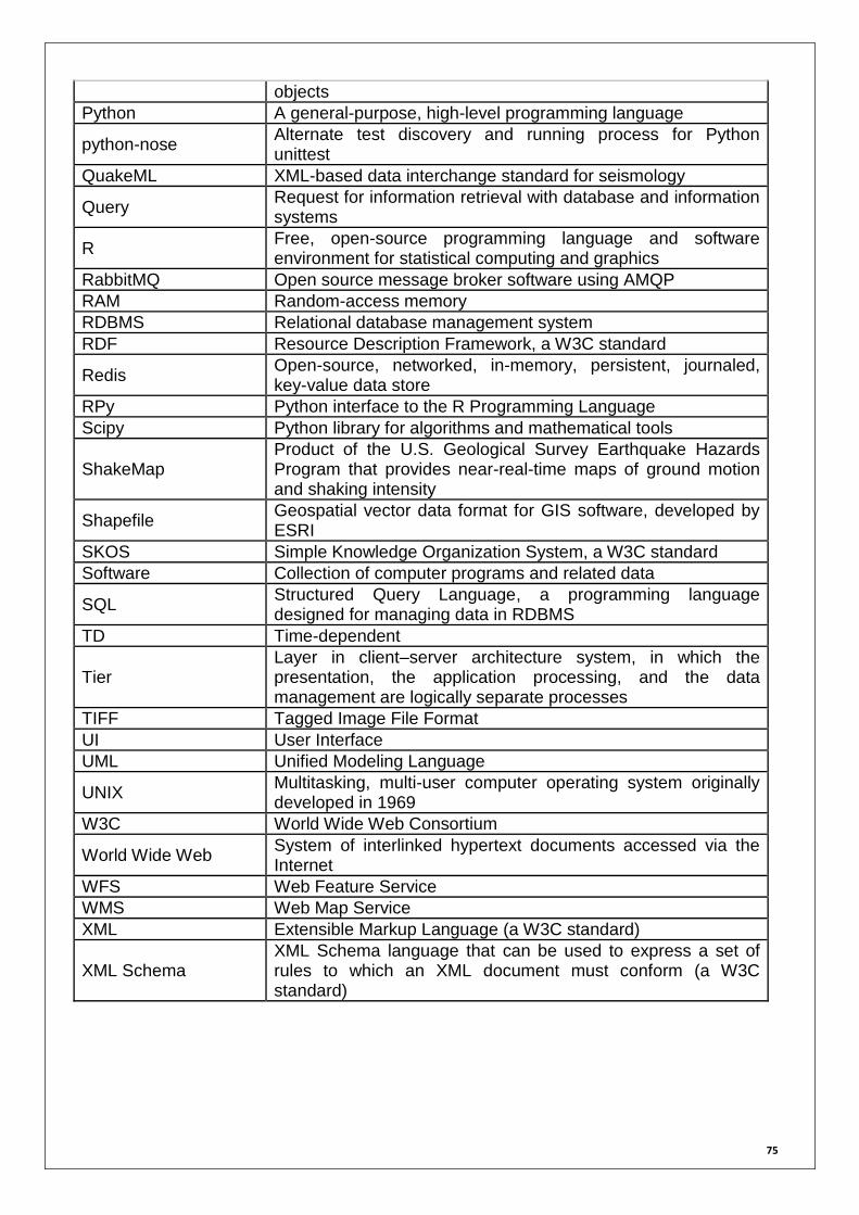
75

objects

Python A general-purpose, high-level programming language

python-nose Alternate test discovery and running process for Python unittest

QuakeML XML-based data interchange standard for seismology

Query Request for information retrieval with database and information systems

R Free, open-source programming language and software environment for statistical computing and graphics

RabbitMQ Open source message broker software using AMQP

RAM Random-access memory

RDBMS Relational database management system

RDF Resource Description Framework, a W3C standard

Redis Open-source, networked, in-memory, persistent, journaled, key-value data store

RPy Python interface to the R Programming Language

Scipy Python library for algorithms and mathematical tools

ShakeMap Product of the U.S. Geological Survey Earthquake Hazards Program that provides near-real-time maps of ground motion and shaking intensity

Shapefile Geospatial vector data format for GIS software, developed by ESRI

SKOS Simple Knowledge Organization System, a W3C standard

Software Collection of computer programs and related data

SQL Structured Query Language, a programming language designed for managing data in RDBMS

TD Time-dependent

Tier Layer in client–server architecture system, in which the presentation, the application processing, and the data management are logically separate processes

TIFF Tagged Image File Format

UI User Interface

UML Unified Modeling Language

UNIX Multitasking, multi-user computer operating system originally developed in 1969

W3C World Wide Web Consortium

World Wide Web System of interlinked hypertext documents accessed via the Internet

WFS Web Feature Service

WMS Web Map Service

XML Extensible Markup Language (a W3C standard)

XML Schema XML Schema language that can be used to express a set of rules to which an XML document must conform (a W3C standard)

76

References Ambraseys, N. N., K. A. Simpson and J. J. Bommer. 1996. Prediction of horzontal

response spectra in Europe. Earthquake Engineering and Structural Dynamics, 25, pp. 371-400

ARMONIA. 2007. Assessing and mapping multiple risks for spatial planning, Approaches, methodologies and tools in Europe. ARMONIA project summary report, 32 pp.

Aspinall, W. P., G. Woo, B. Voight and P. J. Baxter. 2003. Evidence-based volcanology: application to eruption crises. J. Volcanol. Geotherm. Res., 128, doi: 10.1016/S0377-0273(03)00260-9

Baratta, A., G. Zuccaro and A. Binetti. 2004. Strength capacity of a No-Tension portal arch-frame under combined seismic and ash loads. J. Volcanol. Geotherm. Res., 133, doi: 10.1016/S0377-0273(03)00408-6

ByMuR. 2011. The ByMuR software: definition and first steps. Dated 26/06/2011, 3 pp. CAPRA. No date. Hazard Models Review and Selection. Central American Probabilistic

Risk Assessment (CAPRA) initiative, Technical Report Task 1.2, 98 pp. Chiarabba, C., P. De Gori and A. Amato. 2011. Do earthquakes storms repeat in the

Appennines of Italy? Terra Nova, 00, doi: 10.1111/j.1365-3121.2011.01013.x Euchner, F. et al. .2011. NRML: The Natural Hazards’ Risk Markup Language. EGU

abstract no. EGU2011-7097 Gonzalés, M. A., J. R. Marti and P. Kruchten. 2011. A canonical data model for simulator

interoperation in a collaborative system for disaster response simulation. 24th Canadian Conference on Electrical and Computer Engineering, 2011, Niagara Falls, Canada.

Grossi, P., H. Kunreuther and D. Windeler. 2005. Chapter 2 – An Introduction to Catastrophe Models and Insurance. Catastrophe Modeling: A New Approach to Managing Risk. Springer Science+Business Media, Inc., pp. 23-42

Grossi, P. and D. Windeler. 2005. Chapter 4 – Sources, Nature, and Impact of Uncertainties on Catastrophe Modeling. Catastrophe Modeling: A New Approach to Managing Risk. Springer Science+Business Media, Inc., pp. 69-91

Grünthal, G., A. H. Thieken, J. Schwarz, K. S. Radtke, A. Smolka and B. Merz. 2006. Comparative risk assessments for the city of Cologne – Storms, Floods, Earthquakes. Nat. Hazards, 38, 21-44

Gutenberg, B. and C. F. Richter. 1944. Frequency of earthquakes in California. Bull. Seismol. Soc. Am., 34, pp. 184-188

Haugen, E. E. D. and A. M. Kaynia. 2008. A comparative study of empirical models for landslide prediction using historical case histories. 14th World Conference on Earthquake Engineering, Beijing, China, 8 pp.

Hill, D. P., F. Pollitz and C. Newhall. 2002. Earthquake-Volcano Interactions. Physics Today, 55, pp. 41-47

Hochrainer, S., R. Mechler and G. Pflug. 2011. Public Sector Fiscal Vulnerability to Disasters, The IIASA CATSIM Model. Updated book section for J. Birkmann, Ed. 2011. Measuring Vulnerability to Natural Hazards: Towards Disaster Resilient Societies, Tokyo, UNU Press.

Jalayer, F., D. Asprone, A. Prota and G. Manfredi. 2010. A decision support system for post-earthquake reliability assessment of structures subjected to aftershocks: an application to L’Aquila earthquake, 2009. Bull. Earthquake Eng., doi: 10.1007/s10518-010-9230-6

King, G. C. P. 2007. Fault interaction, earthquake stress changes, and the evolution of seismicity. In: Schubert, G. (Ed.), Treatise on Geophysics, Volume 4. Elsevier Ltd., Oxford, pp. 225-256

Lutz, M. 2006. Programming Python, Third Edition. O’Reilly Media, Inc.

77

Mailier, P. J., D. B. Stephenson, C. A. T. Ferro and K. I. Hodges. 2006. Serial clustering of extratropical cyclones. Mon. Wea. Rev., 134, pp. 2224-2240

Marti, J. R., J. A. Hollman, C. Ventura and J. Jatskevich. 2008. Dynamic recovery of critical infrastructures: real-time temporal coordination. Int. J. Critical Infrastructures, 4, pp. 17-31

Marzocchi, W. 1993. The tectonic setting of Mount Vesuvius and the correlation between its eruptions and the earthquakes of the Southern Apennines. J. Volc. Geotherm. Res., 58, pp. 27-41

Marzocchi, W. 2002. Remote seismic influence on large explosive eruptions. J. Geophys. Res., 107, doi: 10.1029/2001JB000307

Marzocchi, W., E. Casarotti and A. Piersanti. 2002. Modelling the stress variations induced by great earthquakes on the largest volcanic eruptions of the 20th century. J. Geophys. Res., 107, doi: 10.1029/2001JB001391

Marzocchi, W., L. Sandri, P. Gasparini, C. Newhall and E. Boschi. 2004. Quantifying probabilities of volcanic events: The example of volcanic hazard at Mount Vesuvius. J. Geophys. Res., 109, doi: 10.1029/2004JB003155

Marzocchi, W., L. Sandri and J. Selva. 2008. BET_EF: a probabilistic tool for long- and short-term eruption forecasting. Bull. Volcanol., 70, doi: 10.1007/s00445-007-0157-y

Marzocchi, W., M. L. Mastellone, A. Di Ruocoo, P. Novelli, E. Romeo and P. Gasparini. 2009. Principles of multi-risk assessment, Interaction amongst natural and man-induced risks. European Commission, Project Report, 72 pp.

Marzocchi, W., L. Sandri and J. Selva. 2010. BET_VH: a probabilistic tool for long-term volcanic hazard assessment. Bull. Volcanol., 72, doi: 10.1007/s00445-010-357-8

Mechler, R., S. Hochrainer, A. Aaheim, H. Salen and A. Wreford. 2010. Modelling economic impacts and adaptation to extreme events: Insight form European case studies. Mitig. Adapt. Strateg. Glob. Change, 15, doi: 10.1007/s11027-010-9249-7

Mignan, A., P. Grossi and R. Muir-Wood. 2011. Risk assessment of Tunguska-type airbursts. Nat. Hazards, 56, doi: 10.1007/s11069-010-9597-3

Muir-Wood, R. and A. Mignan. 2009. A phenomenological reconstruction of the Mw9 Nov 1st 1755 earthquake source. Chapter in The 1755 Lisbon Earthquake: Revisited, Springer, Geotechnical, Geological and Earthquake Engineering, 7, doi: 10.1007/978-1-4020-8609-0_8, ISBN: 978-1-4020-8608-3

Nadim, F., C. Jaedicke, H. Smebye and B. Kalsnes. 2006. Assessment of global landslide hazard hotspots. IPL Project C102, 18 pp.

Nadim, F., H. Einstein and W. Roberds. 2005. Probabilistic stability analysis for individual slopes in soil and rock. 8 pp.

Newhall, C. G. and R. P. Hoblitt. 2002. Constructing event trees for volcanic crises. Bull. Volcanol., 64, doi: 10.1007/s004450100173

Newman, M. E. J. 2005. Power laws, Pareto distributions and Zipf’s law. Contemporary Physics, 46, doi: 10.1080/00107510500052444

Parsons, T. 2005. Significance of stress transfer in time-dependent earthquake probability calculations. J. Geophys. Res., 110, doi: 10.1029/2004JB003190

Rao, A. S., M. D. Lepech, A. S. Kiremidjian and X. Y. Sun. 2010. Time Varying Risk Modeling of Deteriorating Bridge Infrastructure for Sustainable Infrastructure Design. 5th International Conference on Bridge Maintenance Safety Management and Life Cycle Optimization, CRC Press, Taylor & Francis Group, pp. 2494-2501

Risk Management Solutions. 2005. Hurricane Katrina: Profile of a Super Cat, Lessons and Implications for Catastrophe Risk Management. Online report, at www.rms.com/publications/

RiskScape. 2010. RiskScape User Manual. Version 0.2.30, 10 May 2010, 60 pp.

78

Schmidt, J., I. Matcham, S. Reese, A. King, R. Bell, R. Henderson, G. Smart, J. Cousins, W. Smith and D. Heron. 2011. Quantitative multi-risk analysis for natural hazards: a framework for multi-risk modelling. Nat. Hazards, doi: 10.1007/s11069-011-9721-z

Sedan, O. and C. Mirgon. 2003. Application ARMAGEDOM, Notice utilisateur. BRGM/RP-52759-FR, document public, 158 pp.

Selva, J., W. Marzocchi, F. Zencher, E. Casarotti, A. Piersanti and E. Boschi. 2004. A forward test for interaction between remote earthquakes and volcanic eruptions: the case of Sumatra (June 2000) and Denali (November 2002) earthquakes. Earth Planet. Sci. Lett., 226, pp. 383-395

Smolka, A. 2006. Natural disasters and the challenge of extreme events: risk management from an insurance perspective. Phil. Trans. R. Soc. A., 364, 2147-2165, doi: 10.1098/rsta.2006.1818

SYNER-G. 2011. D3.1 – Fragility functions for common RC building types in Europe. Systemic Seismic Vulnerability and Risk Analysis for Buildings, Lifeline Networks and Infrastructures Safety Gain (SYNER-G), March 2011, 209 pp.

Toda, S., R. S. Stein, P. A. Reasenberg, J. H. Dieterich and A. Yoshida. 1998. Stress transferred by the 1995 Mw = 6.9 Kobe, Japan, shock: Effect on aftershocks and future earthquake probabilities. J. Geophys. Res., 103, pp. 24,543-24,565

UBC. 2009. Infrastructure interdependencies simulator (I2Sim), Technical Description and User Manual. Internal report, 37 pp.

USGS. 1996. Probabilistic Seismic Hazard Assessment for the State of California. Open File Report 96-08.

Vangelsten, B. V., S. Lacasse and M. Uzielli. 2007. Probabilistic risk estimation for a Norwegian clay slope. 8 pp.

Vitolo, R., D. B. Stephenson, I. M. Cook and K. Mitchell-Wallace. 2009. Serial clustering of intense European storms. Meteorologische Zeitschrift, 18, pp. 411-424

Vorogushyn, S., B. Merz, K.-E. Lindenschmidt and H. Apel. 2010. A new methodology for flood hazard assessment considering dike breaches. Water Resources Res., 46, doi: 10.1029/2009WR008475

Wells, D. L. and K. J. Coppersmith. 1994. New Empirical Relationships among Magnitude, Rupture Length, Rupture Width, Rupture Area, and Surface Displacement. Bull. Seismol. Soc. Am., 84, pp. 974-1002

Werner, M. J., K. Ide and D. Sornette. 2011. Earthquake forecasting based on data assimilation: Sequential Monte Carlo methods for renewal processes. Nonlinear Proces. Geophys., 18, doi: 10.5194/npg-18-49-2011

Wikle, C. K. and L. M. Berliner. 2007. A Bayesian tutorial for data assimilation. Phys. D Nonlinear Phenom., 230, doi: 10.1016/j.physd.2006.09.017

Yamaguchi, N. and F. Yamazaki. 2000. Fragility curves for buildings in Japan based on damage surveys after the 1995 Kobe earthquake. 12th World Conference of Earthquake Engineering, 2451, pp. 1-8

Zöller, G. and S. Hainzl. 2007. Recurrence Time Distributions of Large Earthquakes in a Stochastic Model for Coupled Fault Systems: The Role of Fault Interaction. Bull. Seismol. Soc. Am., 97, doi: 10.1785/0120060262