projective geometry and camera models
DESCRIPTION
Projective Geometry and Camera Models. ENEE 731 Image Understanding Kaushik Mitra. Camera. 3D to 2D mapping 2D to 3D mapping. Preliminaries. Projective geometry Projective spaces ( P 2 ) Homogenous coordinates Projective transformations (Homography). Why Projective Geometry?. - PowerPoint PPT PresentationTRANSCRIPT
Projective Geometry and Camera Models
ENEE 731 Image Understanding Kaushik Mitra
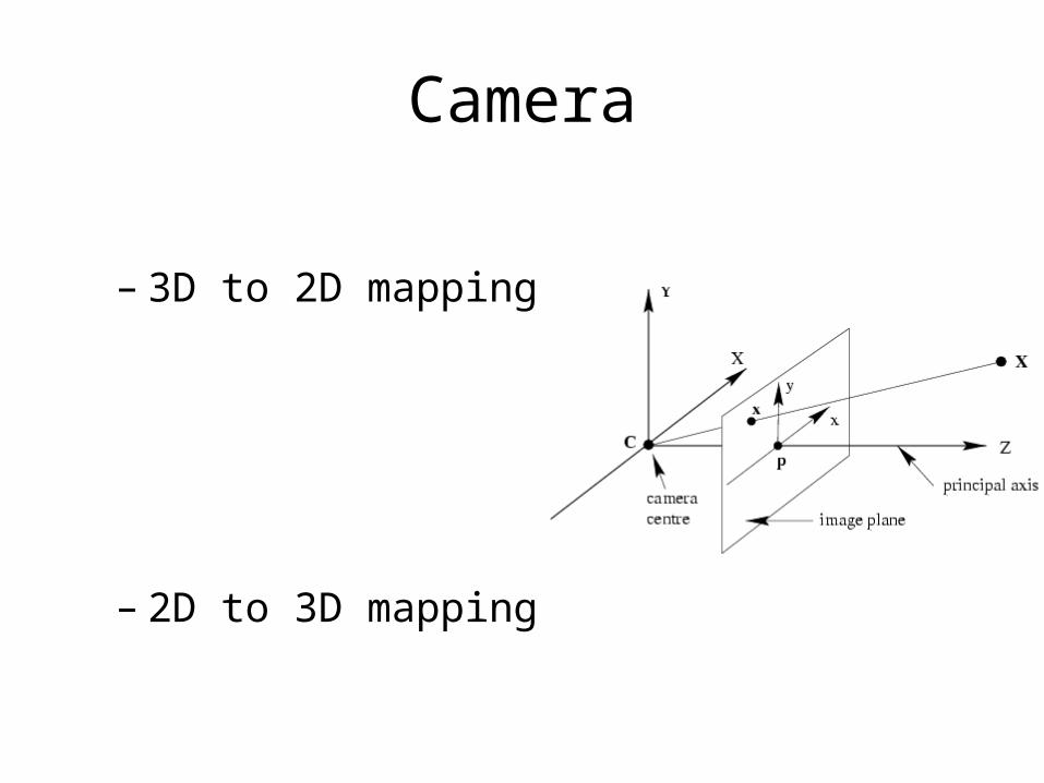
Camera
– 3D to 2D mapping
– 2D to 3D mapping
Preliminaries
• Projective geometry– Projective spaces (P2)– Homogenous coordinates– Projective transformations (Homography)
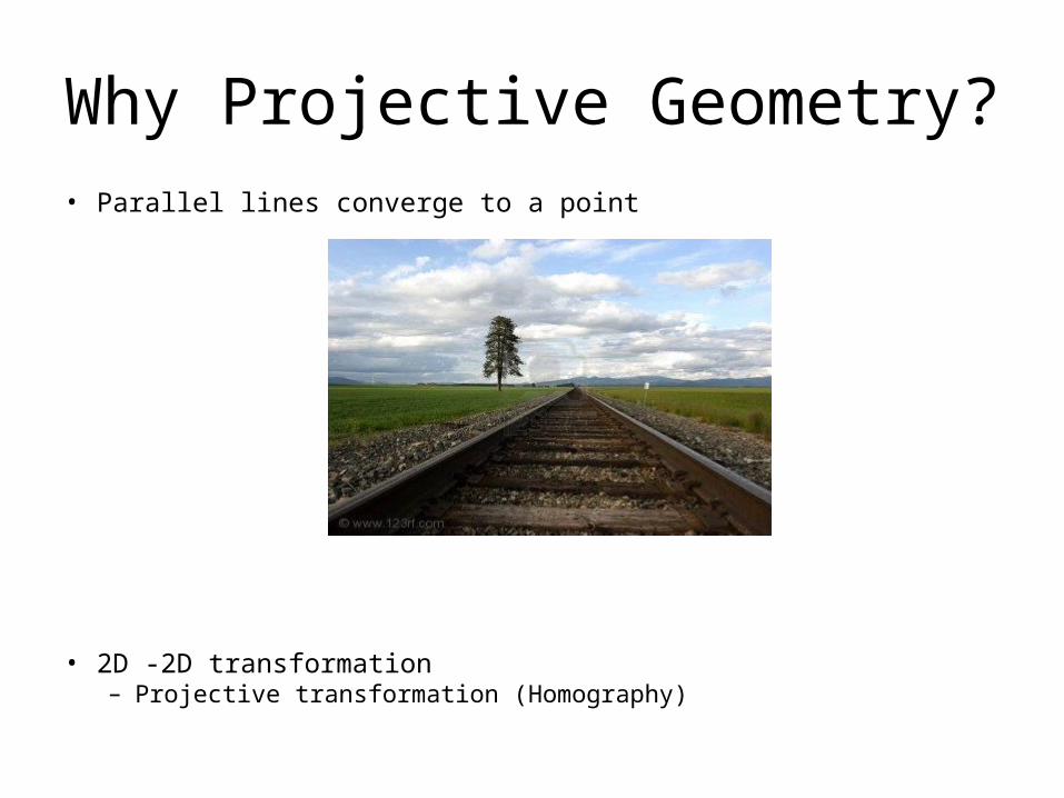
Why Projective Geometry?• Parallel lines converge to a point
• 2D -2D transformation– Projective transformation (Homography)
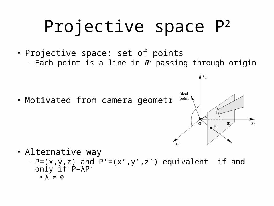
Projective space P2
• Projective space: set of points– Each point is a line in R3 passing through origin
• Motivated from camera geometry
• Alternative way– P=(x,y,z) and P’=(x’,y’,z’) equivalent if and only if P=λP’
• λ ≠ 0
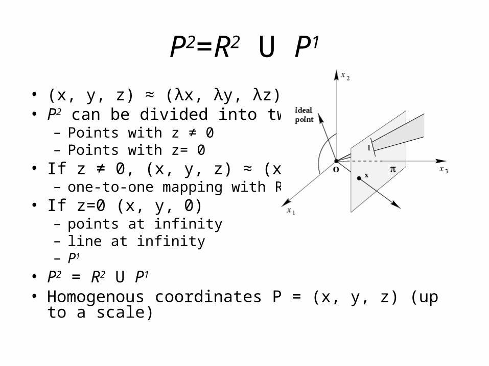
P2=R2 U P1
• (x, y, z) ≈ (λx, λy, λz)• P2 can be divided into two subsets
– Points with z ≠ 0– Points with z= 0
• If z ≠ 0, (x, y, z) ≈ (x/z, y/z, 1) – one-to-one mapping with R2
• If z=0 (x, y, 0) – points at infinity– line at infinity– P1
• P2 = R2 U P1
• Homogenous coordinates P = (x, y, z) (up to a scale)
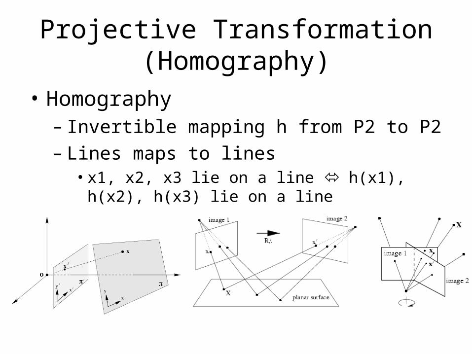
Projective Transformation (Homography)
• Homography– Invertible mapping h from P2 to P2– Lines maps to lines• x1, x2, x3 lie on a line h(x1), h(x2), h(x3) lie on a line
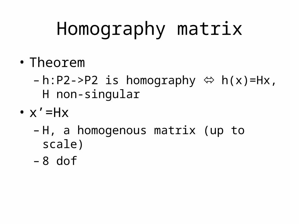
Homography matrix
• Theorem– h:P2->P2 is homography h(x)=Hx, H non-
singular
• x’=Hx– H, a homogenous matrix (up to scale)– 8 dof
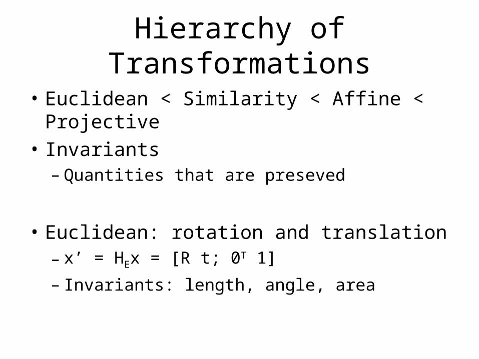
Hierarchy of Transformations
• Euclidean < Similarity < Affine < Projective• Invariants– Quantities that are preseved
• Euclidean: rotation and translation– x’ = HEx = [R t; 0T 1]
– Invariants: length, angle, area
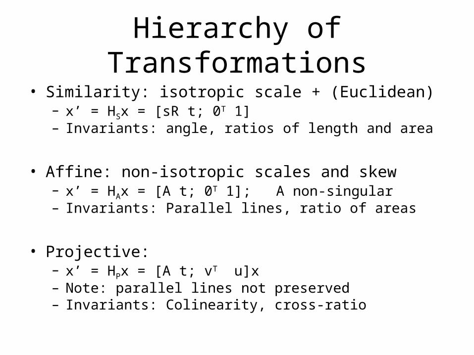
Hierarchy of Transformations• Similarity: isotropic scale + (Euclidean)
– x’ = HSx = [sR t; 0T 1]– Invariants: angle, ratios of length and area
• Affine: non-isotropic scales and skew– x’ = HAx = [A t; 0T 1]; A non-singular– Invariants: Parallel lines, ratio of areas
• Projective: – x’ = HPx = [A t; vT u]x– Note: parallel lines not preserved– Invariants: Colinearity, cross-ratio
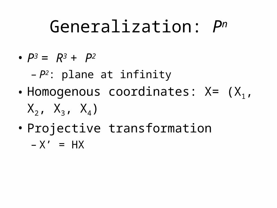
Generalization: Pn
• P3 = R3 + P2
– P2: plane at infinity
• Homogenous coordinates: X= (X1, X2, X3, X4)
• Projective transformation– X’ = HX
Camera Models
Camera Models
• Mapping 3D to 2D: Camera Matrices• Central projection– Pin-hole camera– Finite projective camera
• Parallel projection– Orthographic camera– Affine camera
Pinhole Camera Geometry
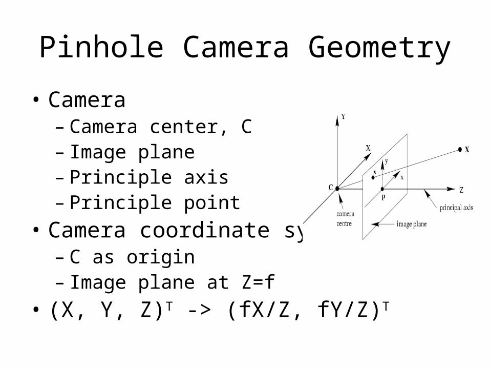
• Camera– Camera center, C– Image plane– Principle axis– Principle point
• Camera coordinate system– C as origin– Image plane at Z=f
• (X, Y, Z)T -> (fX/Z, fY/Z)T
Camera Matrix
• (X, Y, Z)T -> (fX/Z, fY/Z)T
• Homogenous coordinates– (X, Y, Z, 1)T -> (fX, fY, Z)T
• Transformation: diag(f f 1)[I | 0]• Camera projection matrix: x= PX– P = diag(f, f, 1)[I | 0 ], a 3×4 matrix
Principle Point Offset
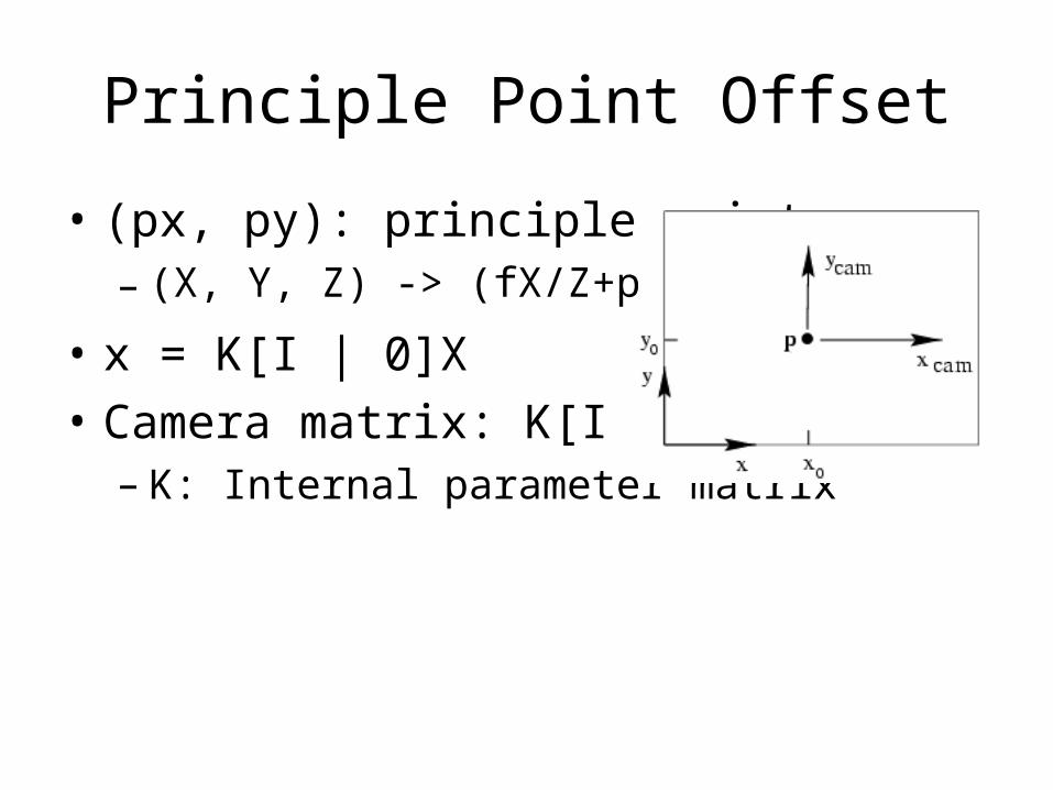
• (px, py): principle point– (X, Y, Z) -> (fX/Z+px, fY/Z+py)
• x = K[I | 0]X• Camera matrix: K[I | 0]– K: Internal parameter matrix
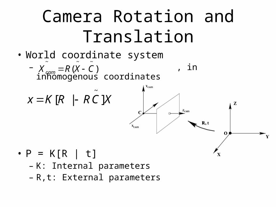
Camera Rotation and Translation
• World coordinate system– , in inhomogenous coordinates
• P = K[R | t]– K: Internal parameters– R,t: External parameters
)(~~~
CXRX cam
XCRRKx ]|[~
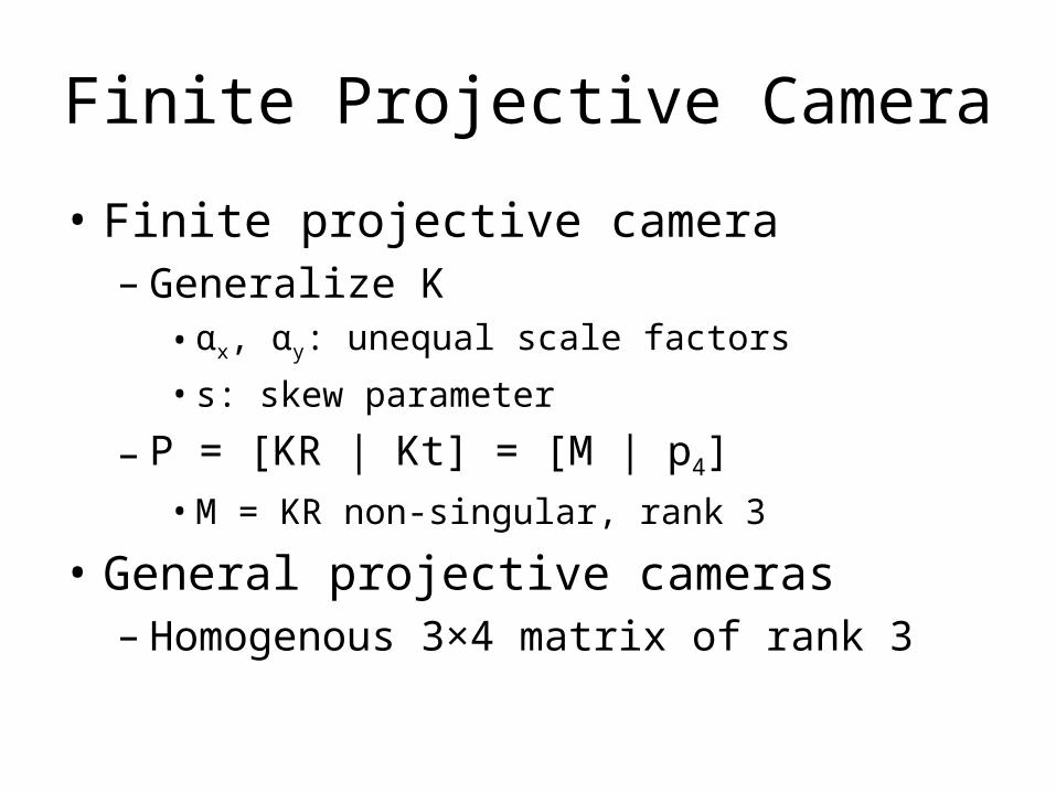
Finite Projective Camera
• Finite projective camera– Generalize K• αx, αy: unequal scale factors
• s: skew parameter
– P = [KR | Kt] = [M | p4]• M = KR non-singular, rank 3
• General projective cameras– Homogenous 3×4 matrix of rank 3
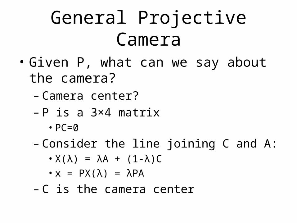
General Projective Camera
• Given P, what can we say about the camera?– Camera center?– P is a 3×4 matrix• PC=0
– Consider the line joining C and A: • X(λ) = λA + (1-λ)C • x = PX(λ) = λPA
– C is the camera center
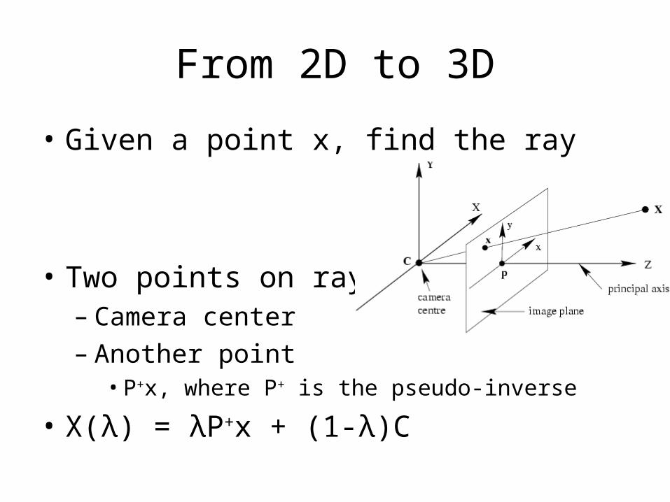
From 2D to 3D
• Given a point x, find the ray
• Two points on ray– Camera center– Another point• P+x, where P+ is the pseudo-inverse
• X(λ) = λP+x + (1-λ)C
Parallel Projection
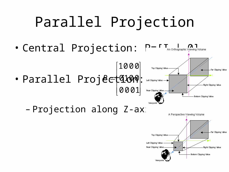
• Central Projection: P=[I | 0]
• Parallel Projection:
– Projection along Z-axis
1000
0010
0001
P
Hierarchy of Parallel Projection
• Orthographic projection• Scaled orthographic projection• Weak perspective projection• Affine projection
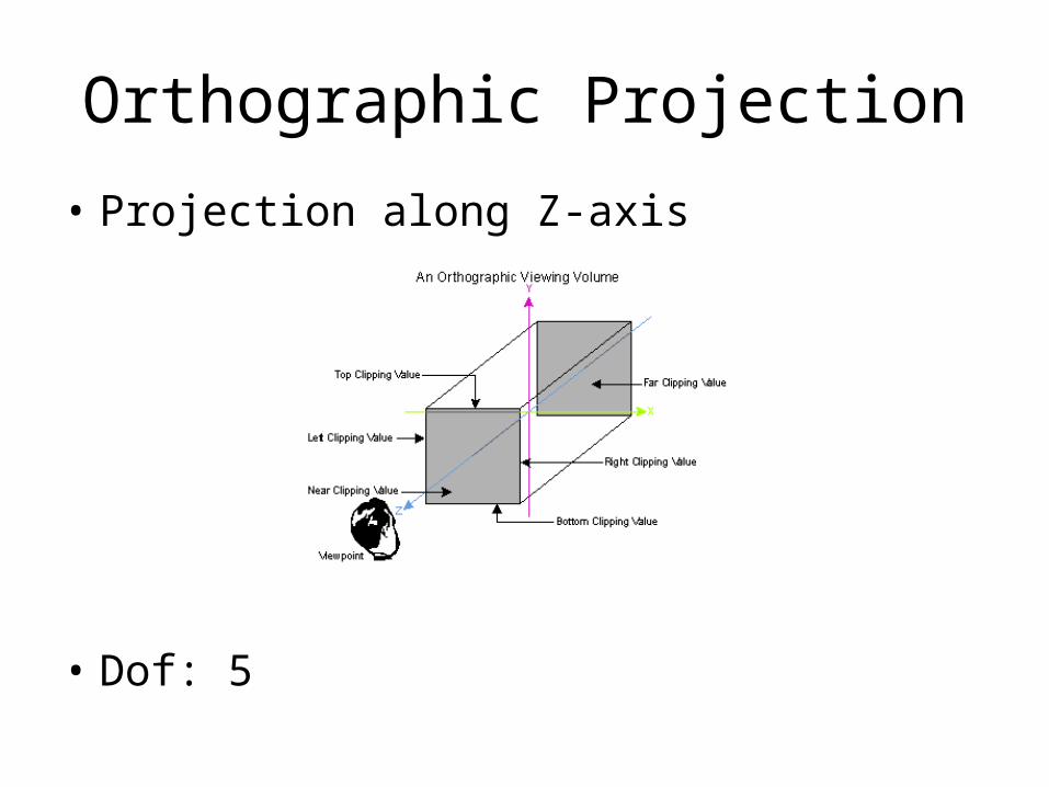
Orthographic Projection
• Projection along Z-axis
• Dof: 5
Generalization of Orthographic Projection (O.P.)
• Scaled orthographic projection– O. P. followed by isotropic scaling– Dof : 6
• Weak perspective projection– O.P. with non-isotropi c scaling– Dof: 7
• Affine camera (projection)– Plus skew – Dof: 8
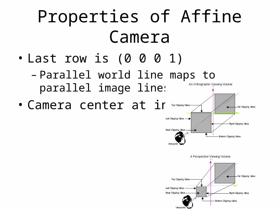
Properties of Affine Camera
• Last row is (0 0 0 1)– Parallel world line maps to parallel image lines
• Camera center at infinity
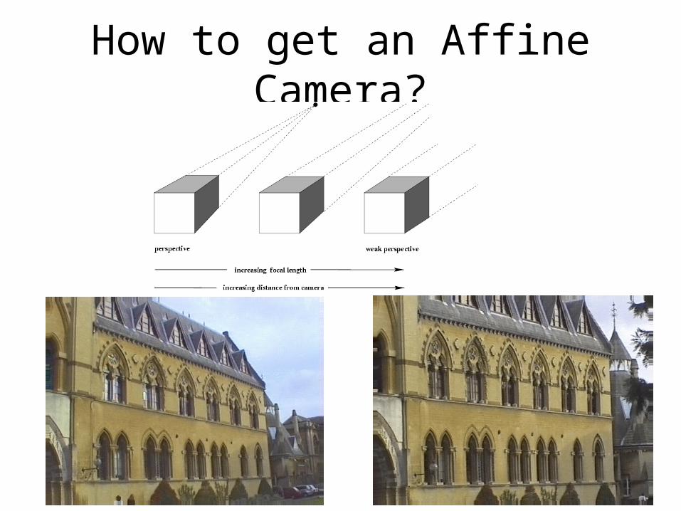
How to get an Affine Camera?
Computation of Camera Matrix P
Approach for Computing P
• x = PX• Estimate P from 3D-2D correspondences– Xi ↔ xi
• Compute K, R, t from P
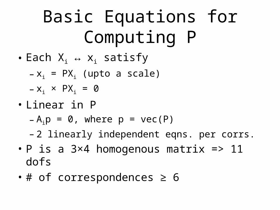
Basic Equations for Computing P
• Each Xi ↔ xi satisfy– xi = PXi (upto a scale)
– xi × PXi = 0
• Linear in P– Aip = 0, where p = vec(P)
– 2 linearly independent eqns. per corrs.
• P is a 3×4 homogenous matrix => 11 dofs• # of correspondences ≥ 6
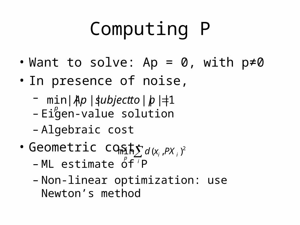
Computing P
• Want to solve: Ap = 0, with p≠0• In presence of noise,– – Eigen-value solution– Algebraic cost
• Geometric cost:– ML estimate of P– Non-linear optimization: use Newton’s method
1||||||||min ptosubjectApp
i
iip
PXxd 2),(min
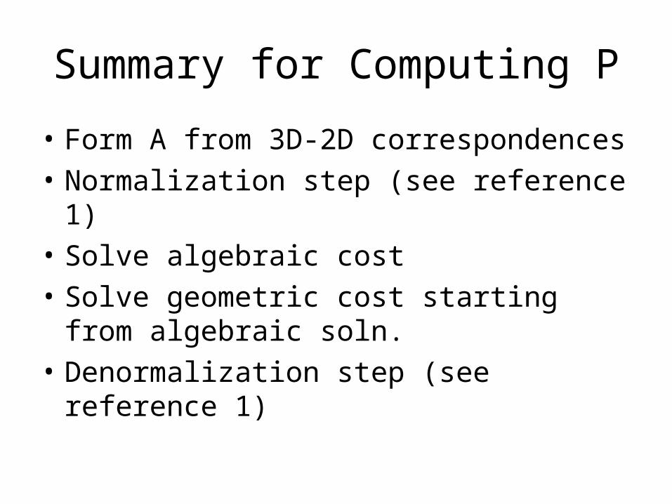
Summary for Computing P
• Form A from 3D-2D correspondences• Normalization step (see reference 1)• Solve algebraic cost• Solve geometric cost starting from algebraic
soln.• Denormalization step (see reference 1)
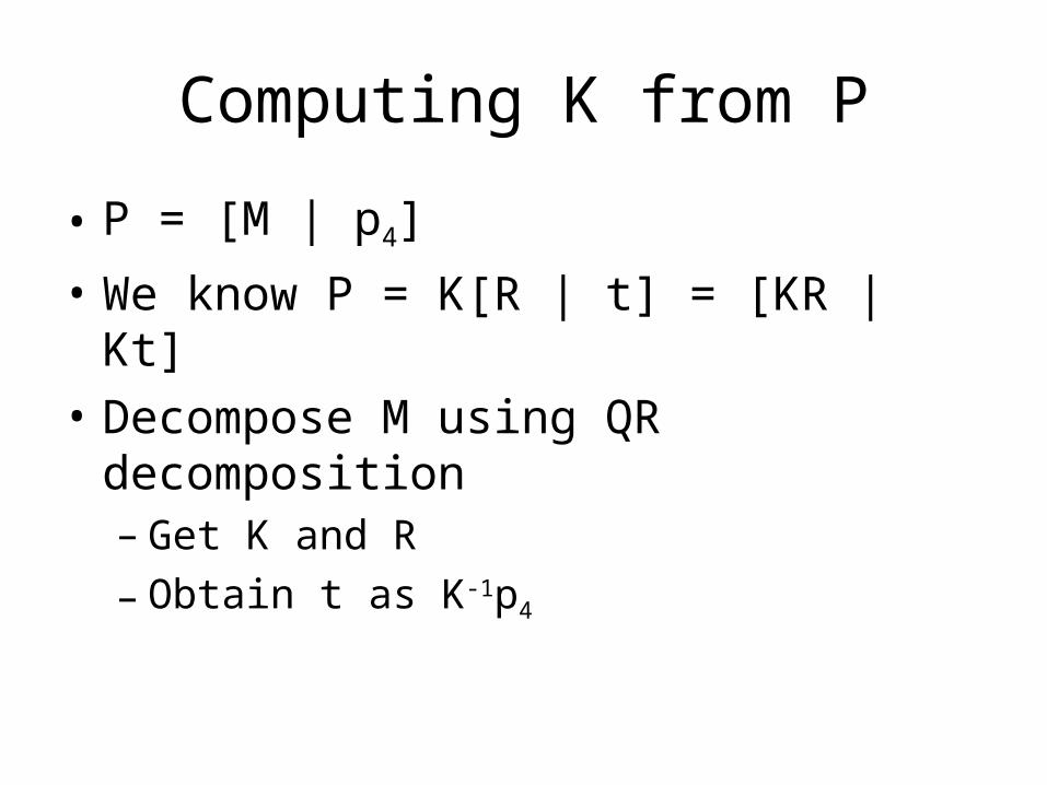
Computing K from P
• P = [M | p4]
• We know P = K[R | t] = [KR | Kt] • Decompose M using QR decomposition– Get K and R– Obtain t as K-1p4
Summary
• Projective geometry: P2 and P3
• Camera models– Central projection (Pin hole camera)– Parallel projection (affine camera)
• Estimation of Camera Model P– Estimation of internal parameter K
References
• 1) Multi-view Geometry (Ch 2, 6, 7)– Hartley and Zisserman
• 2) Computer Vision: Algorithms and Applications– Richard Szeliski