Project TitleCOSMOLOGIES WITH DARK MATTER, DARK

ENERGY & THE MODIFIED GRAVITY(Period : 2013-2016)

Principal Investigator : Bikash Chandra Paul∗

ProfessorPhysics Department, North Bengal University,

Siliguri, Dist. : Darjeeling, Pin : 734 013, West Bengal, India

Abstract

In the project cosmological models have been investigated taking into ac-count modified gravitational sector and/or modified matter sector. The stan-dard BigBang model was the beginning to understand the observed universeimmediately after it was known that the universe is expanding. Hubble’s dis-covery made it clear that we are not living in a static Einstein’s universe.Afterwards it is found that the although BigBang model satisfactorily explainssome of the observed facts of the universe it is entangled with few conceptualproblems which finds no answer in the framework of perfect fluid model. Thenit was claimed that the there exists an inflationary phase of expansion of theuniverse which we need it because of marriage of the particle physics with cos-mology. In 1991, the theoretical cosmological models came up to describe theevolution of the universe may be right from the Planck time. The existenceof such an early inflation is also predicted by Cosmic Background Explorer(COBE). In this context a modification of matter sector i.e., introduction ofscalar field available in standard model of particle physics, instead of isotropicfluid and/or a modification of gravitational sector by Starobinsky came up toobtain early inflation. In 1999, a new phenomena is observed which predictthat the universe is passing through an accelerating phase. In general theoryof relativity (GTR), it came up that once again we need a further modificationof the matter or gravitational sector. Consequently new physics and new con-cepts are needed to understand the observed universe. In view of the recentastronomical and cosmological observations the idea of dark energy and darkmatter is conceived in theoretical framework. In the project the recent issuesin cosmology are probed considering modified gravity or GTR with modifiedmatter sector. It came up that although one can construct a number of cosmo-logical models, some of them are ruled out when analyzed with observations.Recent observed data from astronomical and cosmological observations have

∗Electronic mail : bcpaul@iucaa.ernet.in

1

revealed some novel features of the universe imposing constraints on cosmolog-ical models. A number of observed data in future cosmological missions willhelp further to understand the origin of the universe in a better way.

2

1 Introduction

In modern cosmology, inflation [1, 2, 3, 4, 10, 9, 11, 12] in the early universe is oneof the essential ingredient for constructing a viable cosmological model. Existence ofsuch a phase of inflationary expansion in the early universe is supported from observa-tions of Cosmic Microwave Background Radiation explorer (COBE). The overlappingregion of particle physics and cosmology help us to understood the early universe ina better way. The success of inflationary models [5, 6, 7], in particular, the pre-dicted primordial density fluctuations for the structure formation of the universe isin agreement with the COBE data. In addition it opens up new avenues in the in-terface of particle physics and cosmology leading to new insights both in conceptualand technical issues. The theory of inflation is attractive as it addressed some of thelongstanding problems not understood in the perfect fluid model satisfactorily. Avolume of literature with various cosmological models appeared in the last 30 yearsto understand the origin of the universe. Although it has a number of good features,its mechanism of realization still remains ad hoc.

On the otherhand, the recent observed astronomical and cosmological [16, 17,15, 18, 19] data when interpreted in the context of the Big bang model have pro-vided some interesting information on the composition of fluids in the universe. Theprediction for the composition of the universe namely, dark energy and dark mat-ter in addition to normal matter come from Supernova redshift survey, WilkinsonMicrowave Anisotropy Probe (WMAP), velocity rotational curves in galaxies, thegravitational lensing of galactic clusters [1]. The total energy density may be madeup of three components, baryonic matter 4 %, dark matter 23 % and third part,called dark energy which constitutes the rest 73 % an entirely new kind of fluid notknown in the framework of standard model of particle physics. The present universeis passing once again through an accelerating phase of the universe. As discussed thepresent universe might have emerged from an inflationary era in the very early phaseof the evolution and thereafter the universe passes through radiation dominated andmatter dominated phases. Subsequently recent predictions that the present universeis passing through an accelerating phase. It is not possible to accommodate all thesephases in a single theoretical framework. Moreover, the general theory of relativitywhich is the key theory to understand the universe and its evolution is not enoughfor understanding the observed universe. This is a challenge in theoretical physicsas fields known in the standard model of particle physics are also not enough forunderstanding the present universe although scalar fields can describe the evolutionof the early universe. It is, therefore, demanded that either the gravity sector orthe matter sector requires to be modified. The proper cause of recent acceleration isyet to be understood. It is, therefore, realized that the Einstein field equation withmatter fields permitted by the standard model of particle physics is not enough toaccommodate the accelerating phase. Thus describing universe with present accel-eration is a challenging job for theoretical physics. A number of literature came upwith cosmological model making use of dark energy and dark matter to accommodatepresent accelerating phase but source of the new form of matter remains unknown.We do not know why the universe is still accelerating, but answer to the questiondefinitely will require a new fundamental physics not known yet. In this context weintend to investigate alternative theory considering a modified sector of gravitational

3

and matter sector of the Einstein gravitational action and confront the results ob-tained with the observational data. It may be mentioned here that Starobinsky [2]first obtained inflation in cosmology adding a R2 term in the Einstein-Hilbert actionlong before the efficacy of inflation is known. In the same way a modified gravitywith curvature terms relevant for the present epoch of the universe may be importantto describe the present accelerating phase. Thus cosmological models with modifiedgravity or in the presence of dark matter and dark energy are important to look fora universe that accommodates the present accelerating phase.

1.1 Objective :

The objective of the project is to explore cosmological model which can accommodatethe present accelerating universe in addition to the usual phases of the early universe.The nature of dark matter and dark energy is to be explored considering modifiedtheories of gravity and/or modified matter sector of gravity.

1.2 Methodology :

The Einstein’s general theory of relativity (GTR) is the key equation in understandingthe evolution of the universe. As the recent observations are not fully understood inthe framework of Einstein-Hilbert action. A modified gravitational sector which maybe a correction of GTR and/or a modified matter sector will be employed here. Asthe fields in the standard model confronts with observations in the context of GTRcosmology, new fields possibly new physics from Large Hadron Collider (LHC) maybe needed. In this context a polynomial function of Ricci scalar for gravitationalsector and exotic fields in the case of matter sector are usually prescribed.

In Big bang model a number of issues namely, singularity, existence of quantumgravity region also plagued the model. A model of an ever existing universe (singu-larity free) which eventually enters into the standard big bang epoch at some stageand consistent with the features known today is constructed in [27] which we callemergent universe (EU) model. A flat EU model can be implemented with a com-position of normal and exotic matter permitted by the non-linear equation of state(EOS) p = Aρ−B

√ρ, (A and B are arbitrary constants). The results expected from

PLANCK will be helpful in understanding the EU model in a better way in addition toother cosmological models in various modified theories of gravity. To obtain a viablecosmological model we use observational results and analyze with chi-square mini-mization technique [5]. In the case of non-linear EOS the field equations become verymuch complex to obtain a cosmological solution in known functional form. Therefore,it is convenient to adopt numerical techniques and consequently using Mathematicaand MATLAB, cosmological models have been numerical analysis with the observeddata.

The gravitational action in (3+1) dimensions is given by

I =1

16πG

∫

R√−gd4x+ Im (1)

where G is Newton’s gravitational constant, R is the Ricci scalar, g is the determinantof the metric and Im is the matter action. The Einstein field equation is obtained by

4

varying the above action which is given as

Rµν −1

2gµνR = 8πGTµν (2)

where Rµν , R, gµν , Tµν and G represent the Ricci tensor, Ricci scalar, metric tensor,matter-energy tensor and Newton’s gravitational constant. Here we consider fourdimensions for which µ, ν runs from (0, 1, 2, 3).

We consider a flat Robertson-Walker metric which is given by

ds2 = −dt2 + a2(t)[

dr2 + r2(

dθ2 + sin2θdφ2)]

(3)

where a(t) represents the scale factor of the Universe. We consider the energy mo-mentum tensor as T µ

ν = diagonal(ρ,−p,−p,−p), where ρ is the energy density andp is the pressure. Using the flat Robertson-Walker metric given by eq. (3) in theEinstein’s field equation one obtains

ρ = 3(

a

a

)2

, (4)

p = −[

2a

a+(

a

a

)2]

(5)

where we set G = 18π

and c = 1. The conservation equation is given by

dρ

dt+ 3H (p+ ρ) = 0 (6)

where H = aarepresents the Hubble parameter.

1.3 Results Expected :

Constraints imposed from observational data will hopefully help us to eliminate someof the possible models and facilitate in recognition of probable satisfactory model.

1st Year : Since solution of EU model is already been obtained earlier we willcompare and confront the predictions of this model and F(R) models with the obser-vational data.

2nd Year : We will set up the field equation for a universe with cosmologicalconstant and various matter fields and look for its solution. The experience of thework done in the first year will help us to constrain the choice of matter fields.

3rd year : The complex evolution of the universe, the peculiar change over inthe expansion of the universe will be studied in the context of cosmological modelsconsidered earlier.

2 Problems Investigated

The following works are carried outI. Cosmology• Emergent Universe Model• Evolution of Primordial Black hole• Observational constraints on modified Chaplygin gasII Astrophysics• Compact Objects

5

3 Cosmology I : Emergent Universe Model

In spite of its overwhelming success, modern big-bang cosmology still has some unre-solved issues. The physics of the inflation [1, 9, 10, 11, 12, 13, 14] and the introductionof a small cosmological constant for late time acceleration [15, 16, 17] are not com-pletely understood [20, 21] in details. Moreover, various competing models exist thatare as yet not fully distinguished empirically from the currently available observa-tional data. For this reason there is enough motivation to search for an alternativecosmological model. In this context, Ellis and Maartens [22] considered the possibilityof a cosmological model [23] in which there is no big-bang singularity, no beginningof time, and the universe effectively get rid of a quantum regime for space-time bystaying large at all times. The universe started out in the infinite past in an almoststatic Einstein universe, and subsequently, it entered in an expanding phase slowly,eventually evolving into a hot big-bang era.

The EU scenario merits attention, as it promises to solve several conceptual aswell as technical issues of the big-bang model. A notable direction is regarding thecosmological constant problem [26]. Mukherjee et al. [27] obtained an emergentuniverse in the framework of general theory of relativity in a flat universe with anonlinear equation of state of the form

p = Aρ−B√ρ (7)

where A and B are arbitrary constants. Emergent universe accommodates a latetime de-Sitter phase and thus it naturally leads to the late time acceleration of theuniverse, as well. Such a scenario is promising from the perspective of offering unifiedearly as well as late time dynamics of the universe [39]. Note, however, that the focalpoint of unification in such emergent universe models lies in the choice of the equationof state for the polytropic fluid, while several other models of unification rely moreon the scalar field dynamics through choice of field potentials [40, 41, 42].

The emergent model proposed by Mukherjee et al. [27] gives rise to a universewith a composition of three different types of fluids determined by the parameters Aand B. In the original emergent universe model proposed by Mukherjee et al. [27],it was assumed non-interacting fluids and each of the three types of fluids identifiedsatisfy conservation equations separately. For a viable cosmological scenario, it isfurther necessary to consider a consistent model of the universe which contains radi-ation dominated, matter dominated and subsequently the late accelerated phases ofthe universe. In the original EU model [27], the composition of the universe is fixedonce A is fixed. A problem thus arises as to how a pressureless matter componentcould be accommodated within such a scenario. However, allowing interaction amongthe constituent fluids of the emergent universe may open up richer physical conse-quences. In the present context interaction among the constituent fluids is useful toobtain a consistent evolutionary scenario of the universe. Another important consis-tency condition is imposed through the thermodynamics of an expanding universe.Einstein’s equations have been interpreted as a thermodynamical relation resultingfrom the displacement of the horizon. Since the emergent universe scenario entails aphase of accelerated expansion, it is relevant here to study the status of the second

6

law of thermodynamics in the picture involving interacting fluids in the emergentuniverse.

Two different types of emergent universe scenario are studied: (i) a two-fluidmodel with interaction of the fluid having the non-linear EoS given by eq. (1) withanother barotropic fluid, beginning at some time t = ti (Model-i) and (ii) a three-fluidmodel with interaction among the various constituent fluids with different individualequations of state, starting at a time t = to (Model-ii).

In the original emergent universe [27] a polytropic equation of state (henceforth,EoS) is considered which is

p = Aρ− Bρ1/2 (8)

where A and B are arbitrary constants. Making use of the conservation equation andthe EoS given by eqs. (4) and (5) in eq. (7), one obtains a second order differentialequation given by

2a

a+ (3A+ 1)

(

a

a

)2

−√3B

a

a= 0. (9)

The scale factor of the universe is thus obtained integrating eq. (8) which is given by

a(t) =

[

3K(A+ 1)

2

(

σ +2√3B

e√

32Bt

)] 23(A+1)

(10)

where K and σ are the two integration constants. It is interesting to note that B < 0leads to a contracting universe whereas with B > 0 and A > −1 leads to a non-singular solution which is expanding. The later solution corresponds to an emergentuniverse which was obtained by Mukherjee et. al. [27]. The energy density of theuniverse in terms of scale factor is obtained from eq. (6) making use of EoS given byeq. (7) which is given by

ρ(a) =1

(A+ 1)2

(

B +K

a3(A+1)

2

)2

. (11)

Expanding the above expression, one obtains energy density as the sum of three termswhich can be identified with three different types of fluids. Thus, the components ofenergy density and pressure can be expressed as follows:

ρ(a) = Σ3i=1ρi and p(a) = Σ3

i=1pi (12)

where we denote

ρ1 =B2

(A+ 1)2, ρ2 =

2KB

(A+ 1)21

a3(A+1)

2

, ρ3 =K2

(A+ 1)21

a3(A+1)(13)

p1 == − B2

(A+ 1)2, p2 =

KB(A− 1)

(A+ 1)21

a3(A+1)

2

, p3 =AK2

(A+ 1)21

a3(A+1). (14)

Comparing with the barotropic EoS , one can determine the role of A. For example,A = 1

3leads to a universe with radiation, exotic matter and dark energy, A = 0 leads

to dark energy, exotic matter and dust. Thus once the EoS parameter A is fixed thecomposition of the fluid in the universe gets determined. It is not possible to get auniverse at a later epoch with matter in it. We consider the following two models :

7

Model (i) : The two fluids model

We consider two interacting fluids with densities ρ and ρ′ which can exchangeenergies with each other. One of the fluid with energy density, say ρ is dominated tobegin with satisfying a non-linear EoS given by eq. (1) which leads to an emergentuniverse model. The effect of other fluid in the energy density of the universe isassumed to be important at a later epoch. The pressure of the former fluid is

p = Aρ−Bρ1/2. (15)

where A and B are constants. The other fluid is considered to be barotropic whichis given by

p′ = ω′ρ′ (16)

where ω′ is EoS parameter. The Hubble parameter ((

H = aa

)

) is given by

3H2 = ρ+ ρ′. (17)

In this case exchange of energy between two different fluids is allowed. The interactionmay sets at ti. The two interacting fluids respect a total energy conservation equationand their densities evolve with time as

ρ+ 3H(ρ+ p) = −αρH, (18)

ρ′ + 3H(ρ′ + p′) = αρH (19)

where α represents a coupling parametrizing the energy exchange between the fluids.One may view the above interaction as a flow of energy from first kind of fluid to thesecond one (say, dark matter) beginning at the epoch considered here. Now, usingeq. (14) in eq. (17), we get a first order differential equation which can be integratedto obtain the behaviour of energy density in terms of the scale factor of the universeand the interaction coupling factor. Thus the energy density and pressure for thefluid of the first kind are given by

ρ =B2

(A+ 1 + α3)2

+2KB

(A+ 1 + α3)2

1

a3(A+1+α

3)

2

+K2

(A+ 1 + α3)2

1

a3(A+1+α3), (20)

p = − B2

(A + 1 + α3)2

+KB(A− 1 + α

3)

(A+ 1 + α3)2

1

a3(A+1+α

3 )

2

+(A+ α

3)K2

(A+ 1 + α3)2

1

a3(A+1+α3). (21)

If the interaction is with a pressureless dark fluid i.e., p′ = 0, eq. (18) can beintegrated using eqs. (16) and (19) which determine the total energy density andpressure as follows :

ρtotal = ρ+ ρ′ =B2

A+ 1+

2KB

(A+ 1)21

a3(A+1)

2

+K2

A+ 1

1

a3(A+1), (22)

ptotal = p = − B2

A + 1+

KB(A− 1)

(A+ 1)21

a3(A+1)

2

+AK2

(A+ 1)21

a3(A+1). (23)

8

The equation of state parameter for the second fluid is given by

ω′ =p′

ρ′=

ptotal − p

ρtotal − ρ. (24)

An interesting case emerges when the coupling parameter α = 2 and A = 13. In

this case a universe with dark energy, exotic matter and radiation to begin with(i.e., before the interaction sets in) can transform to a matter dominated phase. Aconsistent scenario of the observed universe in the EU model may be realized in thiscase.

Model (ii) : The three fluids model

The original EU model was obtained in the presence of non-interacting fluids per-mitted by the parameter A in a flat universe case. The corresponding densities andpressures are given by eqs. (13) and (14) respectively. For non-interacting fluids, theEoS parameters for the three fluids permitted above are given by ω1 = −1, ω2 =12(A− 1) , ω3 = A. For 0 ≤ A ≤ 1, it accommodates dark energy, exotic matter and

the usual barotropic fluid. The energy density and pressure of the exotic matter andthat of the barotropic fluids decreases with the expansion of the universe. However,the rate of decrease is different evident from eqs. (13) and ( 14). We assume aninteraction among the components of the fluid in the universe which is assumed to beoriginated at a later epoch (such interactions could arise due to a variety of mecha-nisms [48, 49, 50, 51, 52, 53]). Assuming onset of interaction among the compositionof the fluid at t ≥ to, the conservation equations for the energy densities of the fluidsnow can be written as

ρ1 + 3H(ρ1 + p1) = −Q′, (25)

ρ2 + 3H(ρ2 + p2) = Q, (26)

ρ3 + 3H(ρ3 + p3) = Q′ −Q, (27)

where Q and Q′ represent the interaction terms, which can have arbitrary form, ρ1represents dark energy density, ρ2 represents exotic matter and ρ3 represents normalmatter. In this case Q < 0 corresponds to energy transfer from exotic matter sector totwo other constituents, Q′ > 0 corresponds to energy transfer from dark energy sectorto the other two fluids, and Q′ < Q corresponds to energy loss for the normal mattersector. The case Q = Q′ corresponds to the limiting case where dark energy interactsonly with the exotic matter. It is important to see that although the three equationsare different the total energy of the fluid satisfies the conservation equation together.It is possible to construct the equivalent effective uncoupled model, described by thefollowing conservation equations:

ρ1 + 3H(1 + ωeff1 )ρ1 = 0 (28)

ρ2 + 3H(1 + ωeff2 )ρ2 = 0 (29)

ρ3 + 3H(1 + ωeff3 )ρ3 = 0 (30)

where the effective equation of state parameters are given below:

ωeff1 = ω1 +

Q′

3Hρ1, (31)

9

-1.0 -0.5 0.0 0.5 1.0 1.5 2.0-1.0

-0.5

0.0

0.5

1.0

1.5

2.0

Ω3 = A

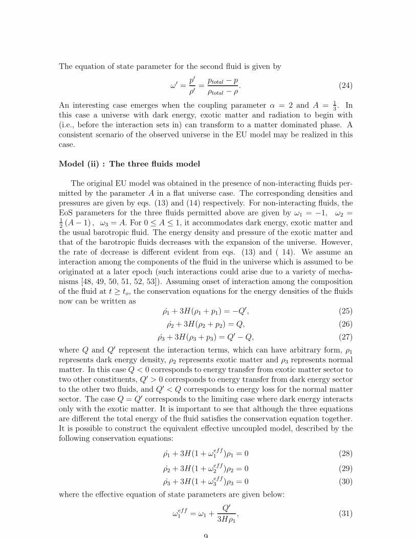
Ω3eff

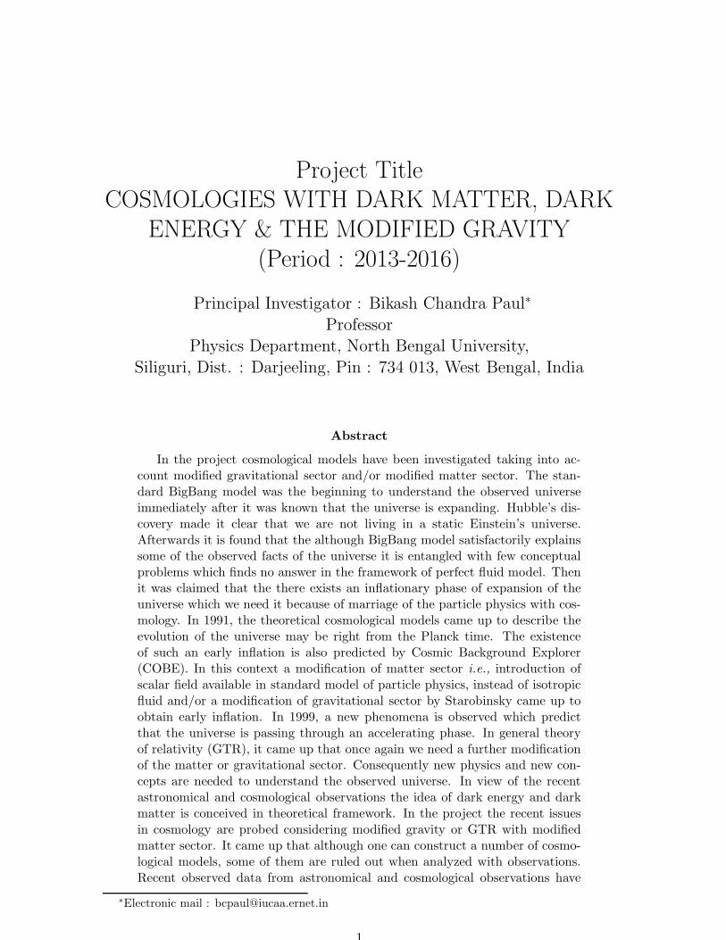
Figure 1: Plot of ωeff3 with EoS parameter A for different interaction β. The thick,

dash, red line and green lines are for β = 0.5, 1, 2, 3 respectively.

ωeff2 = ω2 −

Q′

3Hρ2, (32)

ωeff3 = ω3 +

Q−Q′

3Hρ3. (33)

Now, if we consider the interaction as Q−Q′ = −βHρ3, the effective state parameterfor the normal fluid becomes

ωeff3 = ω3 −

β

3(34)

In fig. 1 we plot the variation of effective equation of state parameter ωeff3 with ω3

(which corresponds to A of the EoS parameter) for different strengths of interactiondetermined by β. We note that as the strength of interaction is increased the valueof ω3 (i.e., A) for which ωeff = 0 (corresponds to matter domination) is found toincrease. Thus a universe with any A value is found to admit a matter dominatedphase at a late epoch depending on the strength of the interaction which was notpermitted in the absence of interaction in an EU model proposed by Mukherjee etal. [27]. It may be pointed out here that in the very early era a universe is assumedwith a composition of three different fluids having no interaction in this picture, thusthe behaviour of the universe at early times remains unchanged as was found in theoriginal EU model. Thus the emergent universe scenario proposed by Mukherjee etal. [27] can be realized in the early era but at a later epoch the composition of matterchanges in the present scenario from its original one with the onset of interaction.This feature represents a clear improvement over the earlier cosmological scenarioin an emergent universe [27, 29, 30] where it is rather difficult to accommodate apressureless fluid.

10

3.1 Concluding Remarks on Emergent Universe Model

Emergent universe scenario is explored in the presence of interacting fluids. Twodifferent cosmological models are Model (i), we consider the flow of energy from thefluids required to realize the emergent universe to a pressureless fluid which sets in atan epoch t = ti. The density of the pressureless fluid assumes importance as mattercomponent after the epoch ti. In Model (ii), we consider interactions among the threefluids of the emergent universe at time t = t0. Before this epoch the emergent universecan be realized without an interaction among the fluids. The problem with earliercosmological realizations of the emergent universe was that once the EoS parameter Ais fixed at a given value, the universe is unable to come out of the phase with a givencomposition of fluids. In the present work we overcome this problem by assigning aninteraction among the fluids at the epoch t0. A cosmological evolution of the observeduniverse through unified dynamics of associated matter and dark energy componentsthus becomes feasible in the emergent universe scenario. It is evident that a earlyuniverse with a radiation dominated phase transits to a matter dominated phasewith all the features observable at the present moment with the onset of interactionconsidered here.

3.1.1 Thermodynamics and EU model

Generalized Second Law of Thermodynamics in an interacting fluid EU Model isexplored considering the universe as a thermodynamical system. We determine theentropy and non-negativity of the time rate of change of Stotal demonstrates thevalidity of the second law of thermodynamics in the context of the emergent universemodel.

3.1.2 On the Origin of Initial Einstein Static Phase

Recently the origin of initial static Einstein universe is explored in massive gravitytheory. A wormhole solution is found in the framework of massive gravity whichpermits such a static universe needed for EU initial phase which however does notpermitted in GTR.

4 Cosmology II : Chaplygin Gas as Modified Mat-

ter sector

In the framework of GTR, ordinary matter fields available in the standard modelof particle physics fails to account for the present observations of the universe. Itis therefore essential to look for a new physics or a new type of matter that in thematter sector of the Einstein-Hilbert action. Chaplygin gas (CG) was considered tobe one such candidate for dark energy. The equation of state (henceforth, EoS) forCG is

p = −A

ρ(35)

11

where A is a positive constant. The initial idea of a CG originated in aerodynamics[64]. But CG is ruled out in cosmology as cosmological models are not consistentwith observations [66, 67]. Subsequently, CG is generalized to incorporate differentaspects of the observational universe known as generalized Chaplygin gas (in short,GCG) [71, 67] which is given by

p = − A

ρα(36)

with 0 ≤ α ≤ 1. It has two free parameters A and α. It is known that GCG is capableof explaining the background dynamics and various other features of a homogeneousisotropic universe satisfactorily. However, the features that the GCG corresponds toalmost dust (p = 0) at high density does not agree completely with our universe. Itis also known that the model suffers from a serious problem at the perturbative level.The matter power spectrum of GCG exhibits strong oscillations or instabilities, unlessGCG model reduces to ΛCDM [73]. The oscillations for the baryonic component withGCG leads to undesirable features in CMB spectrum [74]. In order to use the gasequation in cosmology, further modification is done by adding term linear in densityto the EoS which is known as modified Chaplygin gas (in short MCG). The EoS forMCG is given by:

p = Bρ− A

ρα(37)

where A, B, α are positive constants with 0 ≤ α ≤ 1. The MCG contains one morefree parameter, namely, B, over the GCG. It may be pointed out here that the MCGis a single fluid model which unifies dark matter and dark energy. The MCG model issuitable for obtaining constant negative pressure at low density accommodating lateacceleration, and a radiation dominated era (with B = 1

3) at high density. Thus a

universe with a MCG may be described starting from the radiation epoch to the epochdominated by the dark energy consistently. On the other hand the GCG describesthe evolution of the universe from matter dominated to a dark energy dominatedregime (as B = 0). So compared to GCG, the proposed MCG is suitable to describethe evolution of the universe over a wide range of epoch [76].

Cosmological models are analyzed here using various observational data, namely,the redshift distortion of galaxy power spectra [77], root mean square (r .m.s) massfluctuation (σ8(z)) obtained from galaxy and Ly-α surveys at various redshifts [78, 79],weak lensing statistics [80], Baryon Acoustic Oscillations (BAO) [81], X-ray luminousgalaxy clusters [82], Integrated Sachs-Wolfs (ISW) Effect ([83]-[84]). It is known thatthe redshift distortions are caused by velocity flow induced by gravitational potentialgradient which evolves due to the growth of the universe. The gravitational growthindex γ is an important parameter in the context of redshift distortion which is dis-cussed in Ref. [85]. The cluster abundance evolution, however, strongly depends onr.m.s mass fluctuations (σ8(z)) [86], which will be used here for analysis of cosmo-logical models.

The Hubble parameter in terms of redshift is obtained from Einstein’s field equa-tion with MCG as

H(z) = H0

[

Ωb0(1 + z)3 + (1− Ωb0)[As + (1− As)(1 + z)3(1+B)(1+α)]1

1+α

]12

(38)

12

where Ωb0, H0 represents the present baryon density and Hubble parameter respec-tively. The square of the sound speed is

c2s =δp

δρ=

p

ρ(39)

which reduces to

c2s = B +Asα(1 +B)

[As + (1− As)(1 + z)3(1+B)(1+α) ]. (40)

which is always positive indicating that the perturbation is stable [75].The growth rate of the large scale structures is derived from matter density per-

turbation δ = δρmρm

(where δρm represents the fluctuation of matter density ρm) in the

linear regime [7, 6] is given by

δ + 2a

aδ − 4πGeffρmδ = 0. (41)

The field equations for the background cosmology with MCG are

(

a

a

)2

=8πG

3(ρb + ρmcg), (42)

2a

a+(

a

a

)2

= −8πGωmcgρmcg (43)

where ρb is the background energy density. The state parameter ωmcg for MCG is

ωmcg = B − As(1 +B)

[As + (1− As)(1 + z)3(1+B)(1+α)]. (44)

We now change t variable to ln a in eq. (41) for numerical analysis, which gives

(ln δ)′′+ (ln δ)

′2 + (ln δ)′[

1

2− 3

2ωmcg(1− Ωm(a))

]

=3

2Ωm(a) (45)

where Ωm(a) =ρm

ρm+ρmcg. The effective matter density Ωm = Ωb +(1−Ωb)(1−As)

11+α

[87]. We now change the variable from ln a to Ωm(a) once again, the eq. (45) can beexpressed in terms of the logarithmic growth factor f = d log δ

d log awhich is given by

3ωmcgΩm(1− Ωm)df

dΩm

+ f 2 + f[

1

2− 3

2ωmcg(1− Ωm(a))

]

=3

2Ωm(a). (46)

In a flat universe, the dark energy state parameter ω0 is a constant. For a ΛCDMmodel, γ = 6

11[85, 88], for a matter dominated model regime γ = 4

7[90, 91]. One

can also express γ in terms of redshift parameter z. One such parametrization isγ(z) = γ(0) + γ

′z, with γ

′ ≡ dγdz|(z=0) [93, 94]. It is shown recently [92] that the

parametrization smoothly interpolates a low and intermediate redshift range to ahigh redshift range [95]. We consider the following ansatz

f = Ωγ(Ωm)m (a) (47)

13

where the growth index parameter γ(Ωm) can be expanded in Taylor series aroundΩm = 1 as

γ(Ωm) = γ|(Ωm=1) + (Ωm − 1)dγ

dΩm|(Ωm=1) +O(Ωm − 1)2. (48)

Equation (48) in terms of γ becomes

3ωmcgΩm(1−Ωm) lnΩmdγ

dΩm−3ωmcgΩm(γ−

1

2)+Ωγ

m−3

2Ω1−γ

m +3ωmcgγ−3

2ωmcg+

1

2= 0.

(49)Differentiating once again the above equation around Ωm = 1, one obtains zerothorder term in the expansion for γ which is given by

γ =3(1− ωmcg)

5− 6ωmcg, (50)

this is in consequence with dark energy model with a constant ω0. In the sameway differentiating the expression twice and thereafter by a Taylor expansion aroundΩm = 1, one obtains a first order term in the expansion which is given by

dγ

dΩm|(Ωm=1) =

3(1− ωmcg)(1− 3ωmcg

2)

125(1− 6ωmcg

5)3

. (51)

Substituting it in eq. (48), γ up to the first order term becomes

γ(B, α,As) =3(1− ωmcg)

5− 6ωmcg

+ (1− Ωm)3(1− ωmcg)(1− 3ωmcg

2)

125(1− 6ωmcg

5)3

. (52)

Using the expression of ωmcg in the above, γ may be parametrized in terms of B, α,As and z. We define normalized growth function g as

g(z) ≡ δ(z)

δ(0). (53)

The corresponding approximate normalized growth function obtained from the parametrizedform of f which follows from eq. (47) is given by

gth(z) = exp

[

∫ 11+z

1Ωm(a)

γ da

a

]

. (54)

The redshift distortion parameter β, is related to the growth function f as β = fb,

where b represents the bias factor connecting total matter perturbation (δ) and galaxyperturbations ( δg ) (b = δg

δ) [96, 97, 99, 100]. The values for β and b at various

redshifts are obtained from cosmological observations [96, 98] considering ΛCDMmodel. Here we analyze cosmological models in the presence of MCG using cosmicgrowth function. Various power spectrum amplitudes of Lyman-α forest data in SDSSare also useful to determine β.The Chi-square function for growth parameter f is defined as

χ2f (As, B, α) = Σ

[

fobs(zi)− fth(zi, γ)

σfobs

]2

(55)

14

where fobs and σfobs are observed values. However, fth(zi, γ) is obtained from eqs.(47) and (52). Another probe for the matter density perturbation δ(z) is derivedfrom the redshift dependence of the r.m.s mass fluctuation σ8(z). A new Chi-squarefunction is defined which is given by

χ2s(As, B, α) = Σ

[

sobs(zi, zi+1)− sth(zi, zi+1)

σsobs,i

]2

(56)

where sobs, sth are observed and theoretical values respectively. From the Hubbleparameter vs. redshift data (OHD) [101] another Chi-square χ2

(H−z) function is definedwhich is given by

χ2(H−z)(H0, As, B, α, z) =

∑ [H(H0, As, B, α, z)−Hobs(z)]2

σ2z

(57)

where Hobs(z) is the observed Hubble parameter at redshift (z) and σz is the errorassociated with that particular observation. The total Chi-square function is furtherdefined to analyze which is given by

χ2total(As, B, α) = χ2

f (As, B, α) + χ2s(As, B, α) + χ2

(H−z)(As, B, α). (58)

The best-fit values are obtained first by minimizing the Chi-square function thereafterthe contours are drawn at different confidence limit.

4.1 Results from Numerical Analysis :

The best-fit values of the EoS parameters are obtained minimizing χ2f (As, B, α) mak-

ing use of the growth rate data. The corresponding contours are drawn relatingAs and B. Using the best-fit values of the parameters As, B, α are As= 0.81,B = −0.10, α= 0.02 obtained from analysis are used to determine constraints : (i)0.6638 < As < 0.8932 and −0.9758 < B < 0.1892 at 95.4 % confidence limit.

Using best-fit values of the parameters As= 0.816, B= -0.146, α= 0.004. As, B,α once again in χ2

f (As, B, α)+χ2s(As, B, α), contours are drawn for As with B which

puts the following constraints: (i) 0.6649 < As < 0.896 and −1.5 < B < 0.1765 at95.4 % confidence limit.

Finally, a total Chi-square function χ2tot(As,B,α) is defined and minimizing it the

best fit values are As= 0.769, B= 0.008, α= 0.002 employed to draw contours andthe following limiting values (i) 0.6711 < As < 0.8346 and −0.1412 < B < 0.1502 at95.4 % confidence limit are noted. It is observed that at 2σ level As ( 0.6711 < As <0.8346) admits positive values but B can take either a positive or negative value inthe range (−0.1412 < B < 0.1502). Thus a viable cosmological model is permittedhere with all the three parameters which are positive.

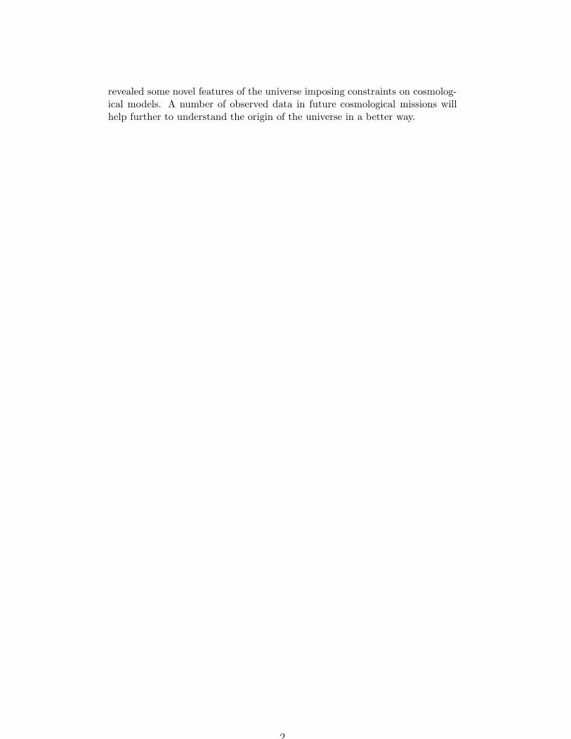
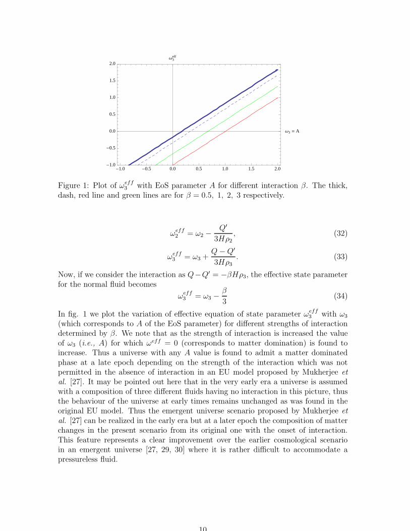
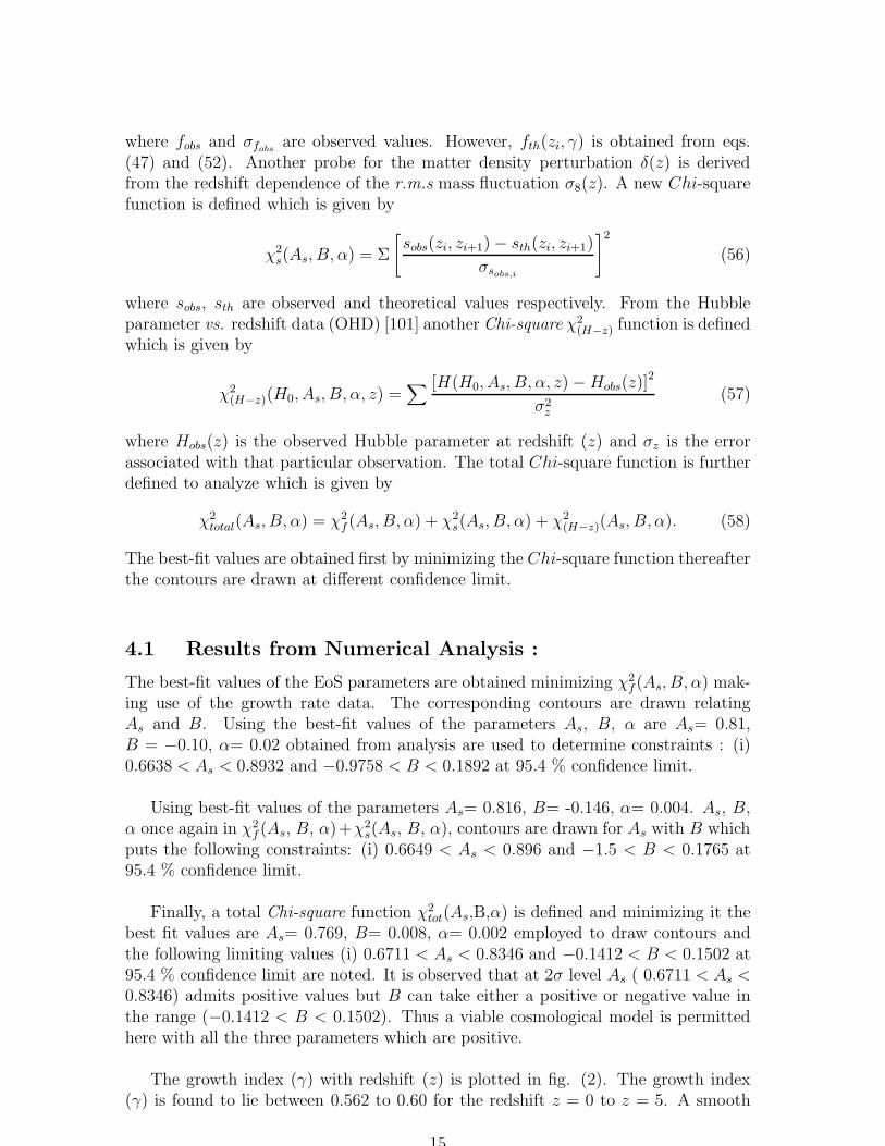
The growth index (γ) with redshift (z) is plotted in fig. (2). The growth index(γ) is found to lie between 0.562 to 0.60 for the redshift z = 0 to z = 5. A smooth

15

1 2 3 4 5z

0.57

0.58

0.59

0.60

Γ

Figure 2: Evolution of growth index γ with redshift at best-fit values: As= 0.769,B= 0.008, α= 0.002

.

1 2 3 4 5z

-0.7

-0.6

-0.5

-0.4

-0.3

-0.2

-0.1

Ω

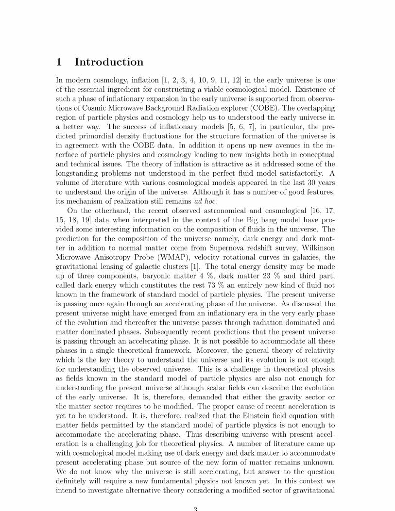
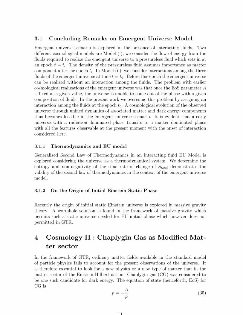
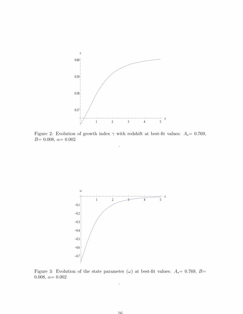
Figure 3: Evolution of the state parameter (ω) at best-fit values: As= 0.769, B=0.008, α= 0.002

.

16

fall of γ at low redshift is noticed.The state parameter (ω) with z is plotted in fig. (3). Here, (ω) varies from -0.767 atthe present epoch (z = 0) to ω → 0 at intermediate redshift (z = 5). The result is insupport of the observation that present universe is now passing through an acceler-ating phase which is dominated by dark energy whereas in the early universe (z > 5)it was decelerating. It is noted that c2s varies between 0.0095 to 0.0080 in the aboveredshift range. A small positive value indicates the growth in the structures of theuniverse.

4.2 Concluding Remarks on MCG Cosmologies

Cosmological models with MCG as a candidate for dark energy is used here to estimatethe range of values of the EoS parameters making use of recent observed data. Thegrowth of perturbation for large scale structure formation in this model is studiedusing the theory. The observed data are employed here to study the growth of matterperturbation and to determine the range of values of growth index γ as consideredin Ref. [86] with MCG similar to the method adopted in Ref. [102]. The modelparameters are constrained using the latest observational data from redshift distortionof galaxy power spectra and the r .m.s mass fluctuation (σ8) from Ly-α surveys. Thegrowth data set including theWiggle-Z survey data are employed here for the analysis.

The best-fit values of the parameters are obtained by minimizing the functionχ2tot(As,B,α) for background growth data. The following constraints are obtained (i)

0.6711 < As < 0.8346 and −0.1412 < B < 0.1502 at 95.4 percent confidence limit.However, in the 2σ level we found that As lies between 0.6711 and 0.8346, with B inbetween −0.1412 and 0.1502. Thus B may be negative. The contours for As vs . B,As vs . α and B vs . α are drawn for growth data, growth+ σ8 data and growth+ σ8

+ H vs . z data. The best-fit value of the growth parameter at present epoch (z = 0)is f= 0.472 with growth index γ= 0.562, state parameter ω=-0.767 and Ωm0= 0.262,which are in good agreement with the ΛCDM model. It is also noted that the growthfunction f varies between 0.472 to 1.0 and the growth index γ varies between 0.562 to0.60 for a variation of redshift from z = 0 to z = 5. In this case the state parameterω lies between -0.767 to 0, square of the sound speed is c2s < 1 always.Here the growth and Hubble data are employed to test the suitability of MCG inFRW universe. It is found that a satisfactory cosmological model emerges permittingpresent accelerating universe. The negative values of state parameter (ω ≤ −1

3) sig-

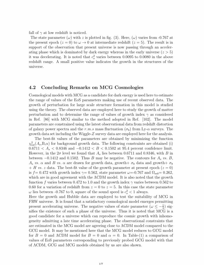
nifies the existence of such a phase of the universe. Thus it is noted that MCG is agood candidate for a universe which can reproduce the cosmic growth with inhomo-geneity admitting a late time accelerating phase. The observational constraints thatare estimated in the MCG model are agreeing close to ΛCDM model compared to theGCG model. It may be mentioned here that the MCG model reduces to GCG modelfor B = 0 and ΛCDM model for B = 0 and α = 0. In Table-(1) a comparison ofvalues of EoS parameters corresponding to previously probed GCG model with thatof ΛCDM, GCG and MCG models obtained by us are also shown.

17

Model Data As α B Ref.GCG Supernovae 0.6-0.85 – 0 [68]GCG CMBR 0.81-0.85 0.2-0.6 0 [69]GCG WMAP 0.78-0.87 – 0 [67]GCG CMBR +BAO ≈ 0.77 ≤ 0.1 0 [70]GCG Growth+ σ8 +OHD 0.708 -0.140 0 this paperMCG Growth+ σ8 +OHD 0.769 0.002 0.008 this paperΛCDM Growth+ σ8 +OHD 0.761 0 0 this paper

Table 1: Comparison of the values of EoS parameters for ΛCDM, GCG and MCGmodels

5 Relativistic Astrophysics

5.1 Relativistic Solutions of Compact Objects and Stellar

Models

In the last couple of decades precision astronomical observations predicted existence ofmassive compact objects with very high densities [104]. The theoretical investigationof such compact astrophysical objects has been a key issue in relativistic astrophysicssince then. In general a white dwarf can be desribed by a polytropic equation ofstate (EOS) which is a less compact star [105]. However, theoretical understandingin the last couple of decades made it clear that there is a deviation from local isotropyof the pressure inside compact objects of high enough densities with smaller radialsize [106, 107]. The physical situations where anisotropic pressure may be relevantare very diverse for a compact stellar object [106, 108, 109, 107]. By anisotropicpressure we mean the radial component of the pressure (pr) different from that of thetangential pressure pt. After the seminal work of Bowers and Liang [109], Rudermanand Canuto [106, 107] theoretically investigated compact objects and observed thata star with matter density (ρ > 1015gm/cc), where the nuclear interaction becomerelativistic in nature, are likely to be anisotropic. It is further noted that anisotropy influid pressure in a star may originate due to number of processes e.g., the existence ofa solid core, the presence of type 3A super fluid etc. [110]. Recently, Mak and Harko[111] determined the maximum mass and mass to radius ratio of a compact isotropicrelativistic star. Bowers and Liang[109], Bayin[112], Maharaj and Maartens [108]examined spherical distribution of anisotropic matter in the framework of generalrelativity and derived a number of solutions to understand the interior of such stars.A handful number of exact interior solutions in general relativity for both the isotropicand the anisotropic compact objects are reported in the literature [113]. Delgaty andLake [113] analysed 127 published solutions out of which they found that only 16 ofthe published results satisfy all the conditions for a physically viable stellar model.In the case of a compact stellar object it is essential to satisfy all the conditionsoutlined by Delgaty and Lake as the EOS of the fluid of the compact dense object isnot known.

Discovery of a handful of compact objects, namely, Her X1, millisecond pulsarSAX J1808.43658, X-ray sources, 4U 1820-30 and 4U 1728-34 led to a belief that

18

these may belong to strange star class. The existence of such characteristics compactobjects led to critical studies of stellar configurations [114, 115, 116, 117, 118, 119, 120,121, 122, 123, 124, 125, 126]. The EoS of matter inside a superdense strange star atpresent is not known. Vaidya-Tikekar [105] and Tikekar [122] have shown that in theabsence of definite information about the EoS, an alternative approach of prescribinga suitable ansatz for the geometry of the interior physical 3-space of the configurationleads to simple easily accessible physically viable models of such stars. Relativisticmodels of superdense stars based on different solutions of Einstein’s field equationsobtained by Vaidya-Tikekar approach of assigning different geometries with physical3-spaces of such objects are reported in the literature [116, 118, 121, 124, 125]. Pantand Sah [127] obtained a class of relativistic static non-singular analytic solutions inisotropic form with a spherically symmetric distribution of matter in a static spacetime. Pant and Sah solution is found to lead to a physically viable causal model ofneutron star with a maximum mass of 4M⊙. Recently, Deb et. al. [128] obtained aclass of compact stellar models using Pant and Sah solution in the case of sphericallysymmetric space time. Further we obtain a class of new relativistic solution whichaccommodates compact objects with anisotropic pressure having mass relevant for aneutron star.

For a static spherically symmetric space time metric given by

ds2 = eν(r)dr2 − eµ(r)(dr2 + r2dΩ2) (59)

where ν(r) and µ(r) are unknown metric functions and dΩ2 = dθ2 + sin2θ dφ2. Thefield equations are

−e−µ

(

µ′′ +µ′2

4+

2µ′

r

)

= ρ, (60)

e−µ

(

µ′2

4+

µ′

r+

µ′ν ′

2+

ν ′

r

)

= pr, (61)

e−µ

(

µ′′

2+

ν ′′

2+

ν ′2

4+

µ′

2r+

ν ′

2r

)

= pt. (62)

Anisotropy is defined as(

µ′′

2+

ν ′′

2+

ν ′2

4− µ′2

4− µ′

2r− ν ′

2r− µ′ν ′

2

)

= ∆eµ. (63)

The above equation is a second-order differential equation which admits a class ofnew solution with anisotropic fluid distribution given by

eν2 = A

1− kα + n r2

R2

1 + kα

, eµ2 =

(1 + kα)2

1 + r2

R2

(64)

where

α(r) =

√

√

√

√

1 + r2

R2

1 + λ r2

R2

(65)

with R, λ, k, A and n are arbitrary constants. The above constants are to bedetermined using the physical conditions imposed on the solutions for a consistent

19

stellar model. For n = 0 recovers the relativistic solution obtained by Pant and Sah[127] for isotropic fluid distribution. The non-zero value of n here corresponds toanisotropic star.

The geometry of the 3-space is given by

dσ2 =dr2 + r2(dθ2 + sin2θdφ2)

1 + r2

R2

. (66)

It corresponds to a 3 sphere immersed in a 4-dimensional Euclidean space. Accord-ingly the geometry of physical space obtained at the t = constant section of the spacetime is given by

ds2 = A2

1− kα + n r2

R2

1 + kα

2

dt2 − (1 + kα)4

(1 + r2

R2 )2

[

dr2 + r2(dθ2 + sin2θdφ2)]

. (67)

For λ > 0, the solution corresponds to finite boundary. The physical properties ofcompact objects filled with anisotropic fluid (n 6= 0) are then studied with differentR, λ, k and A for a viable stellar model. The solutions is also matched with theexterior Schwarzschild line element

ds2 =(

1− 2m

ro

)

dt2 −(

1− 2m

ro

)−1

dr2 − r2o(dθ2 + sin2θdφ2) (68)

at the boundary, where m represents the mass of spherical object. The isotropic formof the metric [5] is

ds2 =

(

1− m2r

1 + m2r

)2

dt2 −(

1 +m

2r

)4

(dr2 + r2dΩ2) (69)

using ro = r(

1 + m2r

)2where ro is the radius of the compact object [5].

5.1.1 Physical properties of anisotropic compact star

The steps for the analysis is outlined below:(1) In this model, a positive central density ρ is obtained for λ < 4

k+ 1.

(2) At the boundary of the star (r = b), the interior solution should be matchedwith the isotropic form of Schwarzschild exterior solution, i.e.,

eν2 |r=b =

(

1− m2b

1 + m2b

)

eµ

2 |r=b =(

1 +m

2b

)2

(70)

(3) The physical radius of a star (ro), is determined knowing the radial distancewhere the pressure at the boundary vanishes (i.e., p(r) = 0 at r = b). The physical

radius is related to the radial distance (r = b) through the relation ro = b(

1 + m2b

)2

[5].(4) The ratio m

bis determined using eqs. (8) and (14), which is given by

m

b= 2± 2A

(

1− kα + ny2√1 + y2

)

. (71)

20

pt

pr

0.00 0.05 0.10 0.15 0.20 0.250.0

0.5

1.0

1.5

2.0

2.5

3.0

r

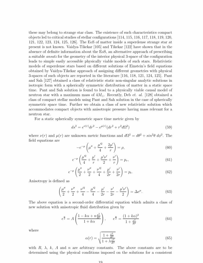
p

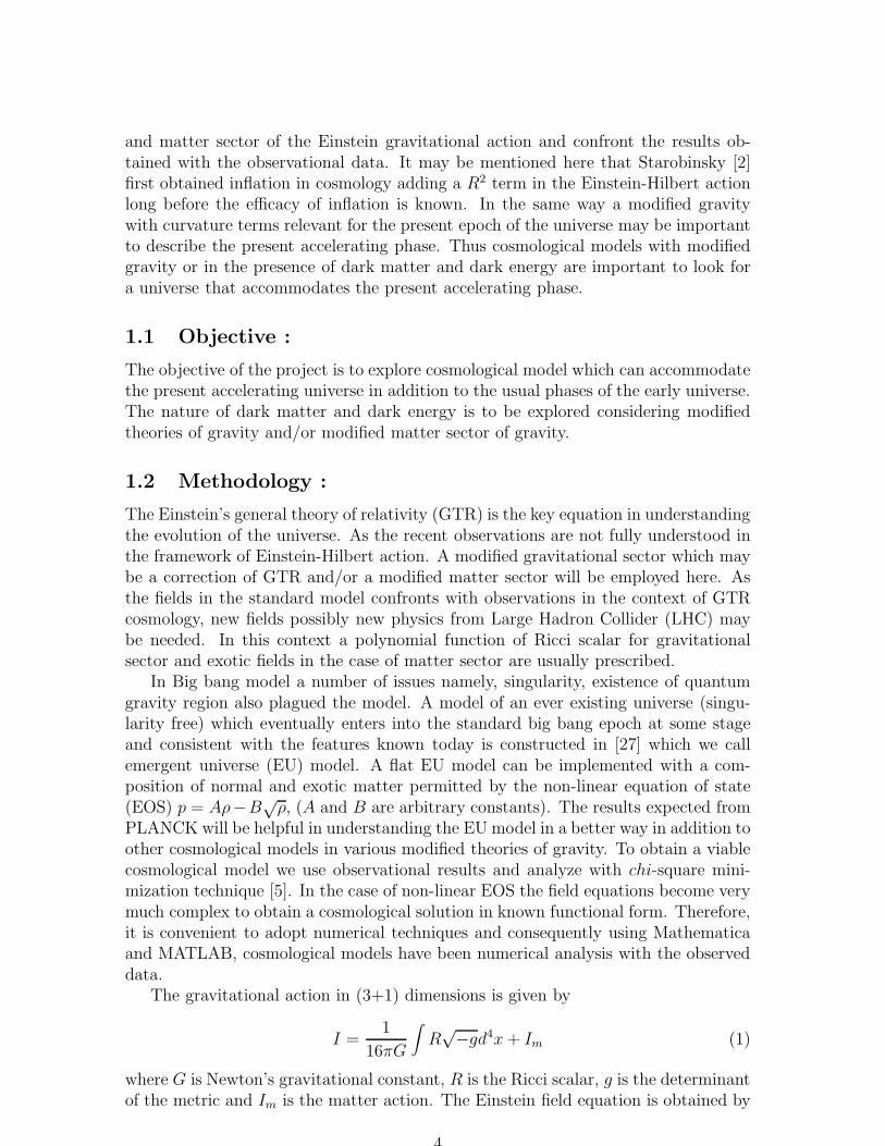
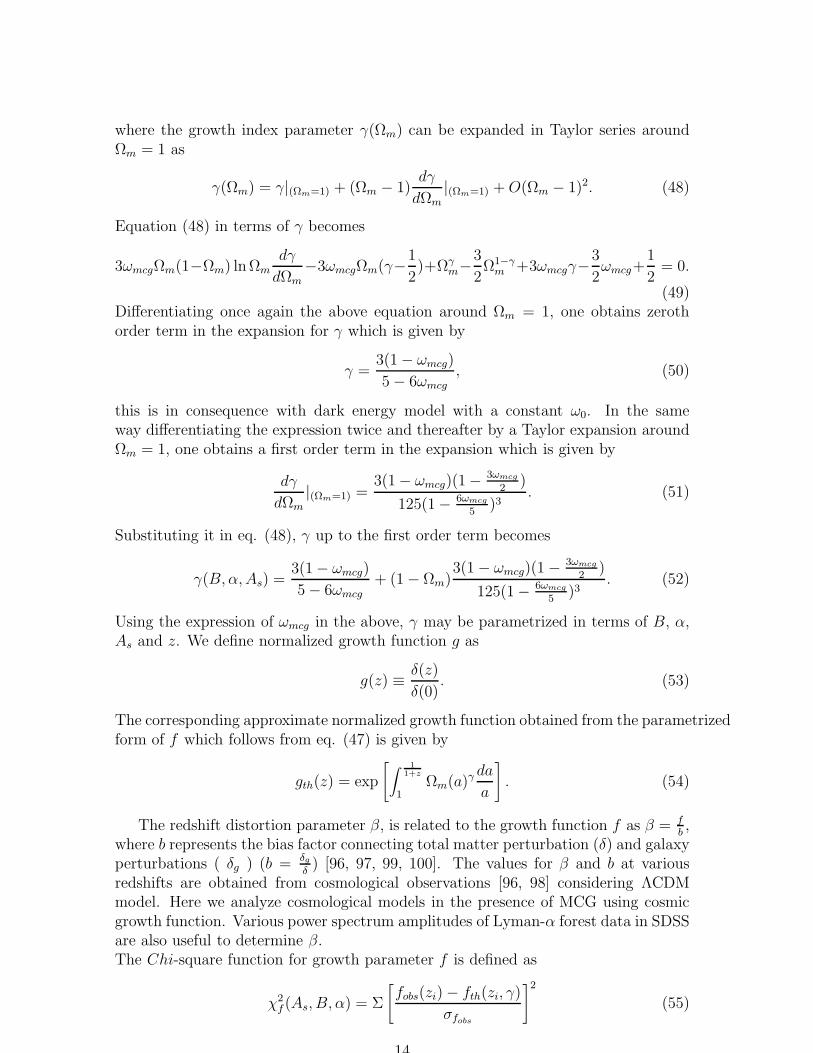
Figure 4: Radial variation of transverse and radial pressure with λ = 10, n = 0.8,A = 2 and k = 0.31. Blue line for radial pressure and red line for transverse pressure.

In the above we consider only negative sign as it corresponds to a physically viablestellar model.

(5) The density inside the star should be positive i.e., ρ > 0.(6) Inside the star the stellar model should satisfy the condition, dp

dρ< 1 for the

sound propagation to be causal.The usual boundary conditions are that the first and second fundamental forms

required to be continuous across the boundary r = b. We determine n, k, λ andA which satisfy the criteria for a viable stellar model outlined above. As the fieldequations are highly non-linear and intractable to obtain a known functional relationbetween pressure and density we adopt numerical technique. Imposing the conditionthat the pressure at the boundary vanishes, we determine y which is given by,

y =b

R(72)

using eq. (5). The square of the acoustic speed dpdρ

becomes :

dp

dρ= −

√α(1 + k

√α)(A+ B√

α+ C +D)

E(73)

where A, B, C, D are functions of r, k, n, λ For given values of λ and k, the size ofthe star is estimated. The mass to radius m

bof a star is then determined, which in

turn determines the physical size of the compact star (ro).The radial variation of pressure and the density of anisotropic compact objects

for different parameters are studied. It is found that radial pressure increases withan increase in k whereas the density decreases. The central density increases with adecrease in k. The pressure inside the star decreases if n is increased, however, densityis independent. The density and pressure are found to increase with an increase in λvalue showing an increase in corresponding central density but the difference betweencentral density with surface density decreases with λ. We also observed that pressureand density do not depend on A. The decrease in radial pressure near the boundaryfalls rapidly for higher values of λ. The variation of radial and transverse pressure

21

0.00 0.05 0.10 0.15 0.20 0.250.00

0.05

0.10

0.15

0.20

r

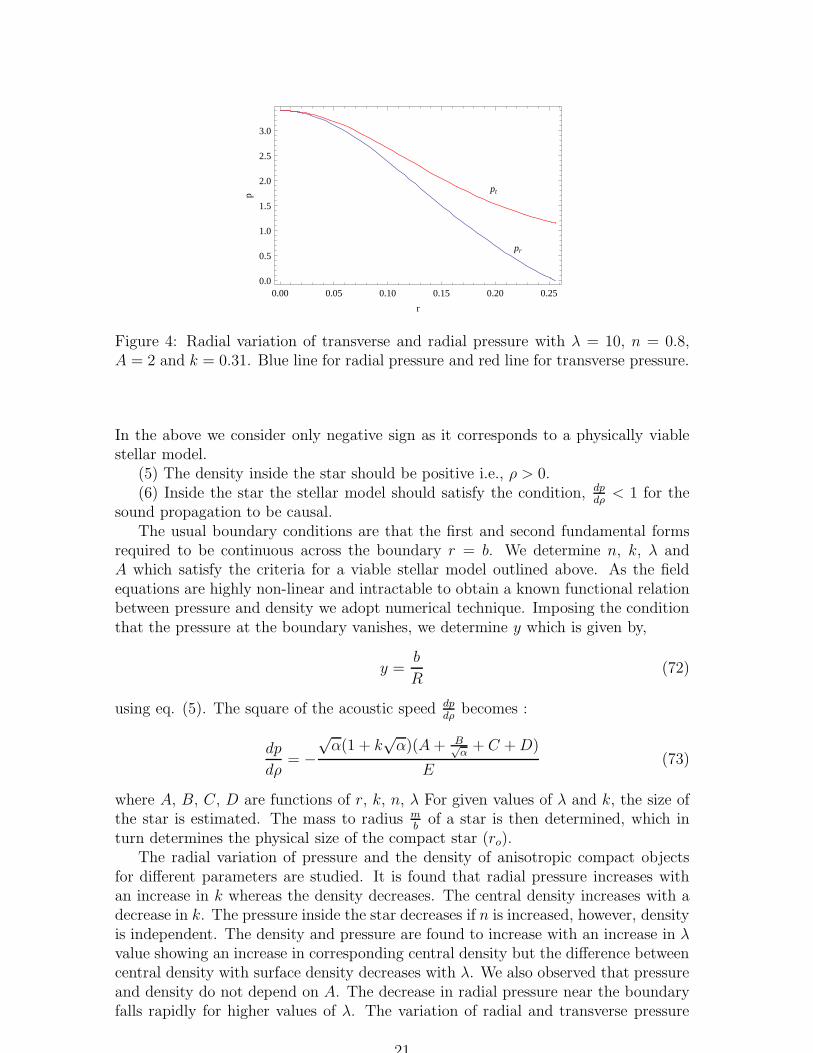
D

Figure 5: Radial variations of anisotropic parameter ∆ for different n. Blue line forn = 0.7 and red line for n = 1.

are plotted in fig. (?), the magnitude of transverse pressure is more than that ofradial pressure although they begin with same central pressure. We note that thereexist a region near the center of the star where strong energy condition (SEC) isnot obeyed. The radius of that region is found to increase with an increase in theparameter values of n, k and λ. Thus the relativistic solution obtained here maybe useful for constructing a core-envelope model of the star. The radial variation ofanisotropy inside the star for different n values are plotted in fig. (13) which showsthat a higher anisotropic star corresponds to a higher values of n.

5.1.2 Stellar Models

For a given mass of a compact star, it is possible to estimate the corresponding radiusin terms of the geometric parameter R. To obtain stellar models we consider compactobjects with observed mass [130] which determines the radius of the star for differentvalues of R with given set of values of n, A, k and λ. It is known that the radius ofa neutron star should be ≤ 10 km., stellar models are obtained here taking differentR so that the size of the star satisfies the upper bound. In the next section weconsider observed masses of compact objects to obtain stellar models. We obtainthree different models using stellar mass data [114, 115, 130] :

Model 1 : For X-ray pulsar Her X-1 [130, 131, 132] characterized by mass m =1.47 M⊙, where M⊙ = the solar mass and found that it permits a star with radiusro = 8.31106 km., for R = 8.169 km. The compactness of the star is u = m

ro= 0.30.

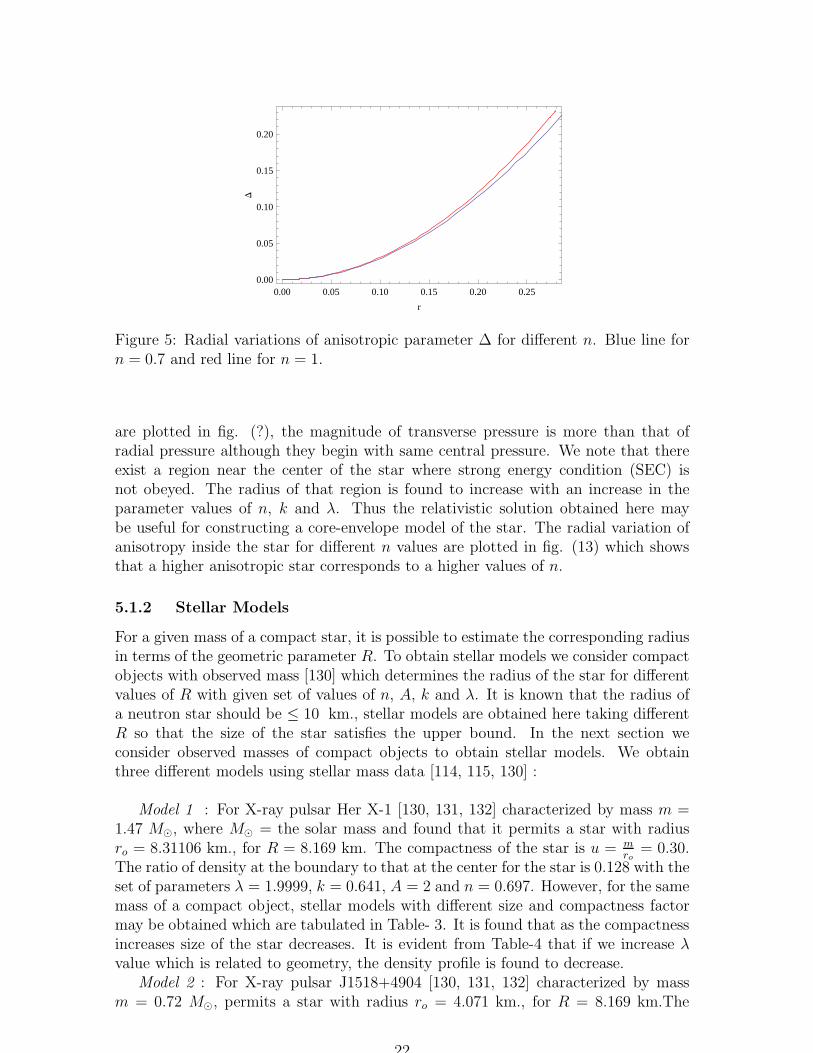
The ratio of density at the boundary to that at the center for the star is 0.128 with theset of parameters λ = 1.9999, k = 0.641, A = 2 and n = 0.697. However, for the samemass of a compact object, stellar models with different size and compactness factormay be obtained which are tabulated in Table- 3. It is found that as the compactnessincreases size of the star decreases. It is evident from Table-4 that if we increase λvalue which is related to geometry, the density profile is found to decrease.

Model 2 : For X-ray pulsar J1518+4904 [130, 131, 132] characterized by massm = 0.72 M⊙, permits a star with radius ro = 4.071 km., for R = 8.169 km.The

22

mb

R in km. Radius (ro in km.)0.3 8.169 8.3110.28 8.574 8.8280.26 9.048 9.4240.25 9.317 9.7570.20 11.096 11.925

Table 2: Variation of size of a star with mbfor k = 0.641, n = 0.697, λ = 1.9999 and

A = 2.

λ 1 1.1 1.2 1.3 1.4 1.5 1.7 1.9999ρ(b)ρ(0)

0.449 0.447 0.444 0.440 0.436 0.432 0.423 0.409

Table 3: Density profile for k = 0.641 , n = 0.697 and A = 2.

compactness of the star in this case is u = mro

= 0.30. The ratio of density at theboundary to that at the centre for the star is 0.142 with λ = 1.1, k = 0.641, A = 2and n = 0.60 .

Model 3 : For B1855+09(g)[130, 131, 132] characterized by mass m = 1.6 M⊙,permits a star with radius ro = 9.047 km., for R = 8.169 km. The compactness ofthe star in this case is u = m

ro= 0.30. The ratio of density at the boundary to that

at the centre for the star is 0.187 with λ = 1, k = 0.52, A = 2 and n = 0.50.

6 Concluding Remarks on Research in Astrophysics

Relativistic solutions of compact objects are obtained using Einstein’s general theoryof relativity and explored the possibility of describing features of very compact objects.In this case primordial black holes are also studied in a modified gravity framework.

6.1 Anisotropic Compact Star

A class of new general relativistic solutions for compact stars which are in hydrostaticequilibrium is obtained assuming anisotropic interior fluid distribution. The radialpressure and the tangential pressure are considered different in this case. As the EOSof the fluid inside a neutron star is not known so we employ numerical technique toobtain a probable EOS of the matter for a given space-time geometry. The interiorspace-time geometry considered here is characterized by five geometrical parametersnamely, λ, R, k, A and n which will be used to obtain stellar models. For n = 0,the relativistic solution reduces to that considered in Refs. [127, 128] to constructstellar models. The permitted range of the values of the unknown parameters aredetermined from the following conditions : (a) metric matching at the boundary, (b)dpdρ

< 1 , (c) pressure at the boundary becomes zero and (d) the positivity of density.

We note the following: (i) The pressure is found to increase with an increase in kbut the density decreases. The central density increases with an decrease in k. (ii)The presssure decreases as n increases, while the density remains unchanged. (iii) The

23

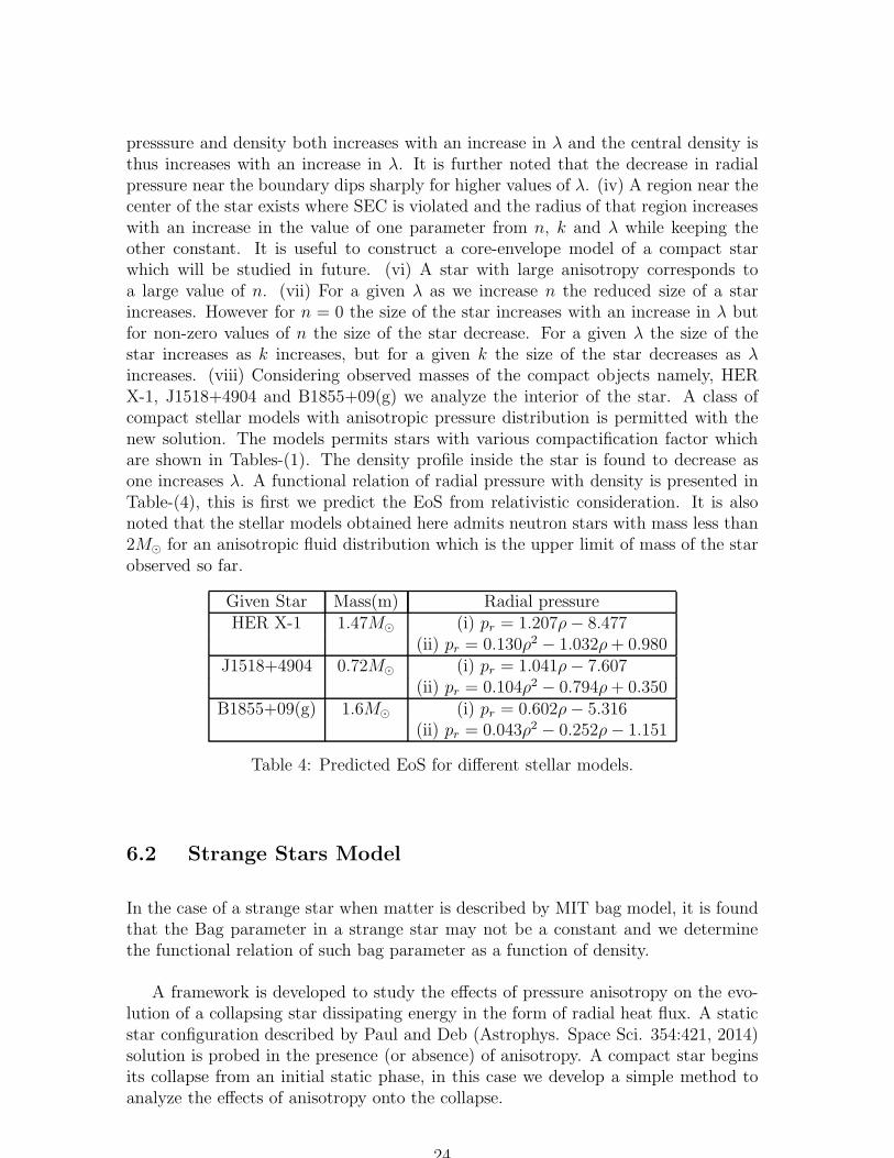
presssure and density both increases with an increase in λ and the central density isthus increases with an increase in λ. It is further noted that the decrease in radialpressure near the boundary dips sharply for higher values of λ. (iv) A region near thecenter of the star exists where SEC is violated and the radius of that region increaseswith an increase in the value of one parameter from n, k and λ while keeping theother constant. It is useful to construct a core-envelope model of a compact starwhich will be studied in future. (vi) A star with large anisotropy corresponds toa large value of n. (vii) For a given λ as we increase n the reduced size of a starincreases. However for n = 0 the size of the star increases with an increase in λ butfor non-zero values of n the size of the star decrease. For a given λ the size of thestar increases as k increases, but for a given k the size of the star decreases as λincreases. (viii) Considering observed masses of the compact objects namely, HERX-1, J1518+4904 and B1855+09(g) we analyze the interior of the star. A class ofcompact stellar models with anisotropic pressure distribution is permitted with thenew solution. The models permits stars with various compactification factor whichare shown in Tables-(1). The density profile inside the star is found to decrease asone increases λ. A functional relation of radial pressure with density is presented inTable-(4), this is first we predict the EoS from relativistic consideration. It is alsonoted that the stellar models obtained here admits neutron stars with mass less than2M⊙ for an anisotropic fluid distribution which is the upper limit of mass of the starobserved so far.

Given Star Mass(m) Radial pressureHER X-1 1.47M⊙ (i) pr = 1.207ρ− 8.477

(ii) pr = 0.130ρ2 − 1.032ρ+ 0.980J1518+4904 0.72M⊙ (i) pr = 1.041ρ− 7.607

(ii) pr = 0.104ρ2 − 0.794ρ+ 0.350B1855+09(g) 1.6M⊙ (i) pr = 0.602ρ− 5.316

(ii) pr = 0.043ρ2 − 0.252ρ− 1.151

Table 4: Predicted EoS for different stellar models.

6.2 Strange Stars Model

In the case of a strange star when matter is described by MIT bag model, it is foundthat the Bag parameter in a strange star may not be a constant and we determinethe functional relation of such bag parameter as a function of density.

A framework is developed to study the effects of pressure anisotropy on the evo-lution of a collapsing star dissipating energy in the form of radial heat flux. A staticstar configuration described by Paul and Deb (Astrophys. Space Sci. 354:421, 2014)solution is probed in the presence (or absence) of anisotropy. A compact star beginsits collapse from an initial static phase, in this case we develop a simple method toanalyze the effects of anisotropy onto the collapse.

24

6.3 PBH in f(T )- Gravity

Black holes are considered as the most elusive object in Astrophysics and cosmology.It is known in stellar physics that Black holes are the ultimate corpse of a collaps-ing massive star when its mass exceeds twice the mass of the sun. Another kind ofblack holes are important in cosmology which might have formed in the early universeduring inflation [133, 134], initial inhomogeneities [135, 136] , phase transition andcritical phenomena in gravitational collapse [137, 138, 139, 140, 141, 142, 143]. Thetopological black holes are formed during inflation due to quantum fluctuations andthey possess mass much smaller than a solar mass. The later type of black holesare popularly known as primordial black holes (in short, PBH). The PBH are im-portant from the Hawking radiation perspective as they are hotter than the cosmicbackground. PBH might play a very important role in contributing total density ofthe universe. The work of Hawking [145] reflected that the black holes emit thermalradiation due to quantum effects which might evaporate, the time scale of evaporationdepends on their masses. It may be that the PBH mass could be small enough forthem to be evaporated completely by the present epoch due to Hawking radiation.Early evaporating PBHs might have contributed for baryogenesis [146, 147, 148]. Onthe otherhand longer lived PBHs could act as seed for the structure formation orgenerating supermassive black hole [149, 150]. It is also possible for the PBHs to sur-vive even longer to date and can contribute a significant component of dark matter[151, 152].

The effect of vacuum energy on the evolution of PBH in GTR is investigated [153]and found that the vacuum energy does not play any role on the evaporating timescale of PBH. The time scale of accretion and the evolution of mass of black holes arestudied in the presence of modified variable Chaplygin gas and viscous generalizedChaplygin gas [154]. In an anisotropic Bianchi-I universe accretion of PBH duringradiation dominated universe is studied [156] and found that the life time is longerthan isotropic universe. Dark matter and density perturbation are studied [157] in thepresence of PBH. [158] studied the large scale structure formation from PBH evapo-ration. The effect of PBH on 21 cm fluctuation is studied recently [159]. PBHs arealso considered as a tool for constraining non-gaussianity [160, 161] in the large scalestructure formations. For understanding further we study PBH in the f(T )-gravity,a modified theory of gravity. We studied the accretion of PBH in f(T ) gravity inthe presence of modified Chaplygin gas. We note that initially accretion dominated,the rate of increase of accretion over evaporation upto a certain epoch is dominating.However at late time, the accretion increases sharply attains a maximum thereafterdecreases. The decrease of mass is due to the fact that the evaporation rate is morethan that of accretion. The mass evaporated from a PBH may contribute to the darkenergy of the universe. A strange situation is noted at z = −1 when suddenly rate ofevaporation of primordial black holes becomes large.

25

7 List of Published Papers : Cosmology & Astro-

physics

1. Paul B C & Thakur P, Observational Constraints on Modified Chaplygin Gasfrom Cosmic Growth JCAP 11 052 (2013)

2. Paul B C, Dark Matter and Dark Energy in the Universe Bibechana 11 421-430 (2014)

3. Panigrahi D, Paul B C & Chatterjee S, Constraining Modified Chaplygin GasParameters Gravitation and Cosmology 356 327-337 (2015)

4. Paul B C & Majumdar A S, Emergent Universe with interacting fluids andGeneralized Second law of Thermodynamics Class. Quantum Grav. 32 115001(2015)

5. Paul B C & Thakur P, Observational Constraints on Chaplygin Gas: A ReviewChapter-7 in An Introduction to Astronomical Data Amnalysis ed: B C Paul 149-177(2015).6. Paul Bikash Chandra & Deb Rumi, Relativistic solutions of Anisotropic CompactObjects Astrophys. & Space Sci. 354 421-430 (2014)

7. Chattopadhyay P K, Deb R & Paul B C , Relativistic charged solutions inHigher Deimensions Int. J. Theor. Phys. 53 1666-1684 (2014)8. Paul B C, Chattopadhyay P K & Karmakar S, Relativistic anisotropic star and itsmaximum mass in Higher Deimensions Astrophys. & Space Sci. 356 327-337(2015)

9. Chattopadhyay P K & Paul B C , Density dependent B parameter of Relativis-tic stars with anisotropy in Pseudo-spheroidal spacetime Astrophys. Space Sci.361 145 (2016)

10. Debnath U & Paul B C, Evolution of Primordial Black hole in f(T )-gravitywith modified Chaplygin gas Astrophys. Space Sci 355 147-153 (2015)

11. Das S, Sharma R, Paul B C & Deb R, Dissipative Gravitational Collapse ofan anisotropic star Astrophys. Space Sci. 361 1 (2016).

8 Acknowledgement:

The Principal Investigator, Prof. B. C. Paul, Physics Department, NBU acknowledgesUniversity Grants Commission (UGC), New Delhi for financial support in executingand finally completing the Major Research Project awarding with a grant (Grant No.F. No. 42-783/2013(SR), dated 13 Feb 2014).

26

References

[1] Guth A H, Phys. Rev. D 23, 347 (1981).

[2] Starobinsky A A, Phys. Lett. 91 B 99 (1980)

[3] Linde A D, Phys. Lett. 108 B 389 (1982)

[4] Linde A D, Inflation and Quantum Cosmology (Academic Press 1990)

[5] Narlikar J V, Introduction to Cosmology (CUP, 1993)

[6] Liddle A R and Lyth D H, Cosmological Inflation and Large Scale structure(CUP, 1998

[7] Padmanabhan T, Theoretical Cosmology Vol III-(CUP, 2002).

[8] Penzias A A and Wilson R W, Astrophys. J. 142 419 (1965)

[9] Sato K, Mon. Not. Roy. Astron. Soc. 195 467 (1981)

[10] Linde A. D., Phys. Lett. 129B 177 (1983).

[11] Albrecht A and Steinhardt P, Phys. Rev. Lett. 48 1220 (1982)

[12] Albrecht A, arXiv:astro-ph/0007247 (2000)

[13] Linde A D, Phys. Lett B 162 281 (1985)

[14] Mukhanov V F and Chibisov G V, JETP Lett 33 532 (1981)

[15] Riess A G et al. , Astron J. 116 1009 (1998)

[16] Perlmutter S et al., Nature 51 391 (1998)

[17] Perlmutter S et al., Astrophys. J., 517 565 (1999)

[18] Bennett C L et al, arXiv: astro-ph/0302207 (2003)

[19] Spergel D N et al., Astrophys. J. Suppl. 148, 175 (2003).

[20] Carroll S M Living Rev. Rel. 4 1 (2001)

[21] Dicke R H, Peebles P J E, Roll P J and Wilkinson D T Astrophys. J. Lett. 142414 (1965)

[22] Ellis G F R, Maartens R, Class. Quant. Grav. 21 223 (2004)

[23] Harrison E R, Mont. Not. Roy. Aston. Soc. 69 137 (1967)

[24] Ellis G F R, Murugan J and Tsagas C G Class. Quant. Grav. 21 233 (2004)

[25] Murlryne D J, Tavakol R, Lidsey J E and Ellis G F R Phys. Rev. D 71 123512(2005)

27

[26] Padmanabhan T and Padmanabhan H, Int. J. Mod. Phys. D 23, 1430011 (2014)

[27] Mukherjee S, Paul B C, Dadhich N K, Maharaj S D and Beesham A Class.Quant. Grav. 23 6927 (2006)

[28] Chimento L, Phys. Rev. D 69 123517 (2004)

[29] Mukherjee S, Paul B C, Maharaj S D and Beesham A, arXive:gr-qc/0505103(2005)

[30] Paul B C and Ghose S, Gen. Rel. Grav. 42 795 (2010)

[31] Banerjee A, Bandyopadhyay T and Chakraborty S, Gen.Rel.Grav. 40 1603(2008)

[32] Banerjee A, Bandyopadhyay T and Chakraborty S Grav. & Cosmology 13 290(2007)

[33] Debnath U Class. Quant. Grav. 25 205019 (2008)

[34] del Campo S, Herrera R and Labrana P, J. Cosmo. Astropart. Physics 30 0711(2007)

[35] Beesham A, Chervon S V and Maharaj S D, Class. Quantum Grav. 26 075017(2009)

[36] Chervon S V, Maharaj S D, Beesham A and Kubasov A, arXiv: 1405.7219 (2014)

[37] Beesham A, Chervon S V, Maharaj S D and Kubasov A, Quantum Matter 2 388(2013)

[38] Beesham A, Chervon S V, Maharaj S D and Kubasov A, Class. Quantum Grav.26, 075017 (2009)

[39] Bag S, Sahni V, Shtanov Y and Unnikrishnan S, JCAP 07 034 (2014)

[40] Majumdar A S, Phys. Rev. D 64 083503 (2001)

[41] Bose N and Majumdar A S, Phys. Rev. D 79 103517 (2009)

[42] Bose N and Majumdar A S, Phys. Rev. D 80 103508 (2009)

[43] Komatsu E et al., Astrophys. J. Suppl., 192 18 (2011)

[44] Marra V, Amendola L, Sawicki I, Valkenburg W, Phys. Rev. Lett. 110 241305(2013)

[45] Paul B C, Thakur P and Ghose S Mon. Not. Roy. Astron. Soc. 407 415 (2010)

[46] Paul B C, Ghose S and Thakur P, Mon. Not. Roy. Astron. Soc. 413 686 (2011)

[47] Ghose S, Thakur P and Paul B C, Mon. Not. Roy. Astron. Soc. 421 20 (2012)

[48] Barrow J D and Clifton T, Phys. Rev. D 73 103520 (2006)

28

[49] Chimento L P, Phys. Rev. D 81 043525 (2010)

[50] Jamil M, Saridakis E N and Setare M R, Phys. Rev. D 81 023007 (2010)

[51] Lip S Z W, Phys. Rev. D 83 023528 (2011)

[52] Costa F E M, Alcaniz J S, Jain D, Phys. Rev. D 85 107302 (2012)

[53] Cotsakis S and Kittou, Phys. Rev. D 88 083514 (2013)

[54] Frolov A V and Kofman L, J. Cosmol. Astropart. Phys. 05 009 (2003)

[55] Danielsson U H, Phys. Rev. D 71 023516 (2005)

[56] Bousso R, Phys. Rev. D 71 064024 (2005)

[57] Cai R G and Kim S P, JHEP 02 050 (2005)

[58] Akbar M and Cai R G, Phys. Rev. D 75 084003 (2007)

[59] Gibbons G W and Hawking S W, Phys. Rev. D 15 2738 (1977)

[60] Jacobson T, Phys. Rev. Lett. 75 1260 (1995)

[61] Padmanabhan T, Phys. Rep. 406 49 (2005)

[62] Paranjape A, Sarkar S, Padmanabhan T, Phys. Rev. D 74 104015 (2006)

[63] Cai R G, Cao L M and Hu Y P, Class. Quantum Grav. 26 155018 (2009)

[64] Chaplygin S, Sci. Mem. Moscow Univ. Math. Phys. 21 1 (1904).

[65] Kamenshchik A, Moschella U, & Pasquier V, Phys. Lett. B 511 265 (2001).

[66] Zhu Z H, Astron. Astrophys., 423 421 (2004)

[67] Bento M C, Bertolami O, & Sen A A, Phys. Lett. B 575 172 (2003)

[68] Makler M, de Oliveira S D and Waga I, Phys. Lett. B 555 1 (2003)

[69] Bento M C, Bertolami O and Sen A A, Phys. Rev. D 67 063003 (2003)

[70] Barriero T, Bertolami O and Torres P, Phys. Rev. D 78 043530 (2008)

[71] Bilic N, Tupper G B & Viollier R D, Phys. Lett. B 535 17 (2001)

[72] Eisenstein D J et al., Astrophy. J. 633 560 (2005); Sen A A, Phys. Rev. D 66043507 (2002)

[73] Sandvik H, Tegmark M, Zaldarriaga M & Waga I, Phys. Rev. D 69 123524(2004).

[74] Amendola L, Finelli F, Burigana C & Caruran D, JCAP 0307 005 (2003).

[75] Xu L, Wang Y & Noh H, Eur. Phys. J. C 72 1931 (2012)

29

[76] Debnath U, Banerjee A $ Chakraborty S, Class. Quant. Grav. 21 5609 (2004)

[77] Hawkins E, et al., Mon. Not. Roy. Astron. Soc. 346 78 (2003)

[78] Viel M, Haehnelt M G & Spingel V, Mon. Not. Roy. Astron. Soc. 354 684 (2004)

[79] Viel M & Haehnelt M G, Mon. Not. Roy. Astron. Soc. 365 231 (2006)

[80] Kaiser N, Astrophys. J. 498 26 (1998)

[81] Eisenstein D J, et al., Astrophy. J. 633 560 (2005)

[82] Mantz A, Allen S W, Ebeling H & Rapetti, Mon. Not. Roy. Astron. Soc. 387179 (2008)

[83] Rees M G & Sciama D W, Nature 217 511 (1968)

[84] Pogosian L, Corasaniti P S, Stephan-Otto C, Crittenden R & Nichol R, Phys.Rev. D 72 103519 (2005)

[85] Linder E V, Phys. Rev. D 72 043529 (2005)

[86] Wang L & Steinhardt P J, Astrophys. J 508 483 (1998)

[87] Li Z, Wu P & Yu H, Ap. J. 744 176 (2012)

[88] Linder E V & Cahn R N, Astropart. Phys. 28 481 (2007)

[89] Linder E V, Astropart. Phys. 29 336 (2008)

[90] Fry J N, Phys. Lett. B 158 211 (1985)

[91] Nesseris S & Perivolaropoulos L, Phys. Rev. D 77 023504 (2008)

[92] Ishak M & Dossett J, Phys. Rev. D 80 043004 (2009)

[93] Polarski D & Gannouji R, Phys. Lett. B 660 439 (2008)

[94] Gannouji R & Polarski D, JCAP 805 018 (2008)

[95] Dossett J, Ishak M, Moldenhauer J, Gong Y & Wang A, JCAP 1004 022 (2010)

[96] Blake C, et al., Mon. Not. Roy. Astron. Soc. 415 2876 (2011)

[97] Tegmark M, et al., Phys. Rev. D 74 123507 (2006)

[98] Di Porto C & Amendola L, Phys. Rev. D 77 083508 (2008)

[99] Ross N P, et al., Mon. Not. Roy. Astron. Soc. 381 573 (2006)

[100] da Angela J, et al., Mon. Not. Roy. Astron. Soc. 383 565 (2008)

[101] Stern D, Jimenez R, Verde L, Kamionkowski M & Adam Stanford S, JCAP1002 008 (2010)

30

[102] Gupta G, Sen S & Sen A A, JCAP 04 028 (2012)

[103] Paul B C, Ghose S & Thakur P, Mon. Not. Roy. Astron. Soc., 413, 686 (2011)

[104] Shapiro S L & Teukolosky S, Black Holes, White Dwarfs and Neytron Stars:The Physics of Compact Objects (Wiley, New York,1983)

[105] Vaidya P C & Tikekar R, J. Astrophys. Astr. 3, 325 (1982)

[106] Ruderman R, Astron. Astrophy. 10, 427 (1972)

[107] Canuto V, Am. Rev. Astron. Astrophy. 12, 167 (1974)

[108] Maharaj S D & Maartens R, Gen. Rel. Grav. 21, 899 (1989)

[109] Bower R L & Liang E P T, Astrophys. J. 188, 657 (1974)

[110] Kippenhahm R & Weigert A, Stellar structure and Evolution (Springer Verlag,Berlin, 1990)

[111] Mak M K & Harko T, Int. J. Mod. Phys. D 13 149 (2004)

[112] Bayin S S, Phy. Rev. D 26 6 (1982)

[113] Delgaty M S R & Lake K, Comput. Phys. Commun. 115 395 (1998)

[114] Dey M, Bombaci I, Dey J, Ray S, Samanta B C, Phys. Lett. B 438, 123 (1998);Addendum: 447 352 (1999); Erratum: 467, 303 (1999)

[115] Li X D, Bombaci I, Dey M, Dey J, Van del Heuvel E P J, Phys. Rev. Lett. 83,3776 (1999)

[116] Knutsen H, Mon. Not. R. Astron. Soc. 232 163 (1988)

[117] Maharaj S D, Leach P G L, J. Math. Phys. 37 430 (1996)

[118] Mukherjee S, Paul B C, Dadhich N, Class. Quantum Grav. 14 3474 (1997)

[119] Negi P S & Durgapal M S, Gen. Relativ. Gravit. 31 13 (1999)

[120] Bombaci I, Phy. Rev. C 55 1587 (1997)

[121] Tikekar R & Thomas V O, Pramana, Journal of Phys. 50 95 (1998)

[122] Tikekar R, J. Math Phys. 31 2454 (1990)

[123] Gupta Y K & Jassim M K, Astrophys. & Space Sci. 272 403 (2000)

[124] Jotania K & Tikekar R, Int. J. Mod. Phys. D 15 1175 (2006)

[125] Tikekar R & Jotania K, Int. J. Mod. Phys. D 14 1037 (2005)

[126] Finch M R, Skea J E K, Class. Quant.Grav. 6, 46 (1989)

[127] Pant D & Sah A, Phys. Rev. D 32 1358 (1985)

31

[128] Deb R, Paul B C, Tikekar R, Pramana Journal of Physics 79 211 (2012)

[129] Rahaman F, Sharma R, Ray S, Maulick R & Karar I, Euro. Phys. J. C 72 2071(2012)

[130] Lattimer J, http://stellarcollapse.org/nsmasses (2010)

[131] Sharma R, Mukherjee S, Dey M, Dey J, Mod. Phys.Letts. A 17 827 (2002)

[132] Sharma R, Maharaj S D, Mon. Not. R. Astron. Soc. 375 1265 (2007)

[133] Carr B J, Gilbert J H & Lidsey J E, Phys. Rev. D 50, 4853 (1994)

[134] Kholpov M Y, Malomed B A & Zeldovich Ya B, Mon. Not. R. Astron. Soc.215 575 (1985)

[135] Carr B J, Astrophys. J. 201 1 (1975)

[136] Hawking S W, Mon. Not. R. Astron. Soc. 152 75 (1971)

[137] Kholpov M Y & Polnarev A, Phys. Lett. 97 B 383 (1980)

[138] Rubin S G, Kholpov M Y & Sakharov A, Gravit. Cosmol. S 6 51 (2000)

[139] Nozari K, Astropart, Phys. 27 169 (2007)

[140] Musco I, Miller J C & Polnarev A G, Class. Quantum Gravit. 26 235001 (2009)

[141] Niemeyer J C & Jedamzik K, Phys. Rev. D 59 124013 (1998)

[142] Niemeyer J C & Jedamzik K, Phys. Rev. Lett. 80 5481 (1999)

[143] Jedamzik K & Niemeyer J C, Phys. Rev. D 59 124014 (1999)

[144] Kodama H, Sasaki M & Sato K, Prog. Theor. Phys. 68 1979 (1982)

[145] Hawking S W, Commun. Math. Phys. 43 199 (1975)

[146] Copeland E J, Kolb E W & Liddle A R, Phys. Rev. D 43 977 (1991)

[147] Majumdar A S, Dasgupta P & Saxena R P, Int. J. Mod. Phys. D 4 517 (1995)

[148] Upadhyay N, Dasgupta P & Saxena R P, Phys. Rev. D 60 063513 (2008)

[149] Dokuchaev V I, Eroshenko Y N, Rubin S G, Astronomy Reports 52 779 (2008)

[150] Mack K J, Ostriker J P & Ricotti M, Astrophys . J. 665 1277 (2007)

[151] Blais D, Bringmann T, Kiefer C & Polarski D, Phys. Rev. D 67 024024 (2003)

[152] Barrau A, Blais D, Boudoul G & Polarski D, Ann. Phys. (Leipzig) 13 115 (2004)

[153] Nayek B & Jamil M, Phys. Lett. B 709 118 (2012)

[154] Jamil M, Euro. Phys. J. C 62 609 (2009)

32

[155] Jamil M, Qadir A & Ahmad Rashid M, Euro. Phys. J. C 58 325 (2008)

[156] Mahapatra S & Nayek B, arXiv: 1312.7263 (2013)

[157] Fujita T, Harigaya K & Kawasaki M, Phys. Rev. D 88 123519 (2013)

[158] Fujita T, Harigaya K, Kawasaki M & Matsuda R, Phys. Rev. D 89 103501(2014)

[159] Tashiro H & Sugiyama N, arXiv:1207.6405 (2012)

[160] Byrnes C T, Copeland E J & Green A M, Phys. Rev. D 86 043512 (2013)

[161] Young S & Byrnes C T, JCAP 08 052 (2013)

33