projet de traitement du signal : détection de transitoires sur des

Projet de Traitement du Signal :Détection de transitoires sur des signaux d’alimentation

électrique d’avion

4 avril 2013

1 IntroductionSur un avion, l’usure des gaines d’isolation des cables d’alimentation électriques (figure 1) peut

engendrer un phénomène de conduction entre phases. Cela provoque l’apparition d’arcs qui sepropagent le long des cables (phénomène d’“arc tracking”). Ce phénomène est précédé de faiblesperturbations des signaux électriques (transitoires, cf. figure 2) qui doivent être détectés le plustôt possible afin de changer les circuits avant que les équipements ne soient endommagés.

Fig. 1 – Usure des gaines d’isolation

0 500 1000 1500 2000 2500−60

−50

−40

−30

−20

−10

0

10

20

30

40Tension filtree

Echantillons

V

Fig. 2 – Transitoire visible sur un signal de tension filtré

1

Ce projet concerne la détection des transitoires sur des signaux de tension. Le réseau électriquede l’avion sera assimilé au réseau d’alimentation terrestre à 50 Hz. Le phénomène qui nous intéresseaffecte les signaux à des fréquences supérieures à 500 Hz. C’est pourquoi on applique aux signauxun filtrage passe-haut afin de mettre en évidence les transitoires, qui sont très peu énergétiques parrapport au signal à 50 Hz. On procède alors à la détection de transitoires sur les signaux filtrés :pour chaque période de 1

50 = 20ms, le détecteur donne une décision binaire : 1 si un transitoireest détecté, 0 sinon. La chaine de traitement est illustrée en figure 3.

On commencera par générer un signal synthétique à partir d’hypothèses sur les signaux réels.On travaillera par la suite sur ce signal, ainsi que sur les signaux de tension réels fournis dansles fichiers transitoire.mat (avec transitoires) et sig_ref.mat (sans transitoire). L’analyse spec-trale et temporelle des signaux nous permettra de nous orienter vers des méthodes de détectionappropriées. On étudiera ici deux détecteurs, l’un temporel, et l’autre fréquenciel.

0010100111...Détecteur

Filtre passe−haut

tension Décisions par période

Fig. 3 – Chaine de traitement

2 Modélisation d’un signal synthétique avec transitoireLe réseau électrique de l’avion est alternatif, à la fréquence f0 = 50Hz. La tension varie entre

-220V et +220V. La fréquence d’échantillonnage de la sonde est de fe = 2500 éch/s.

1. Générer un signal sinusoïdal d’amplitude 220 (V) à la fréquence f0 échantillonné à la fré-quence fe sur 50 périodes.

2. Ajouter à cette sinusoïde pure un bruit blanc gaussien de moyenne nulle et de variancev0 = 1.

3. On modélise un transitoire par un saut de variance : ajouter à la 20ème période du signalun bruit gaussien de variance 10v0 .

3 Analyse spectraleDéterminer le spectre du signal synthétique et du signal réel donné dans transitoire.mat, à

l’aide des méthodes suivantes (voir annexe 1) :

1. PériodogrammeCalculer le périodogramme du signal en utilisant les fenêtres rectangulaire et de Hamming.

2. CorrélogrammeDéterminer les estimations biaisée et non biaisée de la fonction d’autocorrélation du signal(fonction xcorr.m). En déduire une estimation par corrélogramme de la densité spectrale depuissance du signal et comparer les résultats avec ceux de 1.

Remarque : On utilisera la fonction load.m pour récupérer les données du fichier.

4 Filtrage des signauxLa fréquence fondamentale (raie en f0 dans le spectre) et ses éventuelles harmoniques masquent

les transitoires qui sont beaucoup moins énergétiques. Afin de les détecter plus facilement, on

2

48 48.5 49 49.5 50 50.5 51 51.5 52−4

−2

0

2

4

6

8

10

12

14x 10

6 DSP SIGNAL NON FILTRE (fondamental)

frequence

periodogrammecorrellogramme non biaisecorrellogramme biaise

Fig. 4 – Analyse spectrale d’un signal sinusoïdal par différentes méthodes

supprime ces composantes à l’aide d’un filtre passe-haut. On trouvera en annexe 2 quelques rappelssur le filtrage analogique et numérique.

1. Calculer la réponse impulsionnelle (b0, b1, ..., b2N ) d’un filtre non récursif passe-haut idéal, defréquence de coupure fc = 500Hz, échantillonnée à la fréquence fe et tronquée sur 2N +1 =61 coefficients. On utilisera la méthode de la fenêtre présentée en annexe.

2. Synthétiser ce filtre, et observer sa réponse à l’aide de la fonction freqz.m.3. Procéder au filtrage en utilisant la fonction filter.m. Que peut-on dire des N premiers points

du signal filtré à l’aide de cette fonction ? Afin d’accentuer l’atténuation dans la bandecoupée, on filtrera le signal deux fois consécutives. On filtrera le signal synthétique, puis lesignal réel (fichier transitoire.mat).

4. Comparer (dans les domaines temporel et fréquenciel) les signaux avant et après filtrage.

5 Un détecteur temporel : le détecteur d’énergieOn fait les hypothèses suivantes sur la nature du signal filtré en présence/absence de transitoire :

xn ∼ N(0, σ2

0

)sous hypothèse H0 (pas de transitoire)

xn ∼ N(0, σ2

1

)sous hypothèse H1 (transitoire)

(1)

1. On dispose d’un signal de référence donné dans sig_ref.mat, dont on sait qu’il ne comporteaucun transitoire (hypothèse H0). Observer la distribution statistique de ce signal, aprèsfiltrage passe-haut. On pourra utiliser la fonction histfit.m qui trace l’histogramme d’unvecteur de points ainsi que la gaussienne approchant au mieux leur distribution. Cela est-ilcohérent avec (1) ? Estimer la variance σ2

0 du signal de référence filtré (fonction var.m).2. Le détecteur d’énergie est le détecteur de Neyman Pearson sous les hypothèses gaussiennes

exprimées ci-dessus. Calculer le rapport de vraisemblance de la v.a. (xn) et montrer que ledétecteur de Neyman Pearson peut s’exprimer ainsi :

H0 rejetée si T (x) =∑

n

x2n > γ

où le seuil de détection γ dépend de la probabilité de fausse alarme PFA souhaitée et de lavaleur de σ0. On remarquera que σ1 n’intervient pas dans le calcul du seuil. Cependant, laprobabilité de détection des transitoires sera d’autant plus grande que σ1 est élevé.

3

3. Quelle est la loi de la statistique de test T (X) sous l’hypothèse H0 ?On rappelle que si (x1, x2, ..., xL) sont L variables aléatoires gaussiennes indépendantes, demoyenne nulle et de variance σ2, alors 1

σ2

∑Ln=1 x2

n est distribuée selon une loi du χ2 à Ldegrés de liberté.

4. Calculer le seuil de détection γ pour une probabilité de fausse alarme fixée PFA = 10−15

en utilisant la valeur de σ20 connue a priori (signal synthétique) ou estimée sur le signal de

référence.Remarque : Pour inverser la loi du χ2 on pourra utiliser la fonction chi2inv.m (plus d’info :help chi2inv).

5. Appliquer l’algorithme de détection sur chaque période du signal modélisé et du signal réel.6. Sur le signal transitoire.mat, procéder à l’analyse spectrale du signal filtré, sur des périodes

où l’algorithme détecte. Que peut-on en déduire sur les transitoires ? Le détecteur d’énergieutilise-t-il les propriétés fréquentielles des transitoires ?

7. Sous-échantillonner d’un facteur 2 une période du signal (filtré) où un transitoire est détecté.Observer le spectre du signal sous-échantillonné. Que remarque-t-on ? Expliquer.

5 10 15 20 25 300

0.5

1

1.5

2

2.5x 10

4 DETECTEUR D’ENERGIE

periodes de signal

statistique de testseuil de detection

500 600 700 800 900 1000 1100 1200−40

−20

0

20

40

echantillons du signal

signal filtresauts de variance detectes

Fig. 5 – Détection d’un transitoire

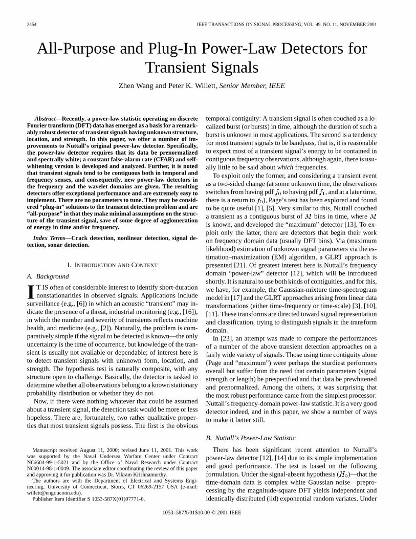
6 Un détecteur fréquentiel : le détecteur de NuttallLe détecteur de Nuttall utilise les propriétés spectrales du transitoire à détecter. Le principe

de ce détecteur est présenté dans [1], partie I. On étudiera ici le détecteur original non normalisé.

1. Montrer que lorsque ν = 1, le détecteur de Nuttall est exactement équivalent au détecteurd’énergie.

2. Montrer que la loi de la statistique de test de Nuttall sous hypothèse H0 peut être approximéepar une loi normale. Les paramètres σ0 et µ0 de cette loi seront estimés à l’aide du signal deréférence (mean.m pour estimer la moyenne d’un signal, var.m pour la variance).

4

3. Montrer qu’on peut exprimer la relation entre µ0, σ0, la probabilité de fausse alarme PFA

et le seuil de détection de Nuttall γnut par :

PFA = QN(µ0,σ0) (γ)

où :

QN(µ0,σ0) (u) =∫ +∞

u

1√2πσ2

0

e− (t−µ0)2

2σ20 dt.

4. Implanter le détecteur de Nuttall avec ν = 2 et pour une probabilité de fausse-alarmePFA = 10−15.Pour le calcul du seuil de détection, on pourra utiliser la fonction norminv.m qui inversela fonction de répartition fµ,σ (ou cdf : cumulative density function) de la loi normale. On

rappelle que si x ∼ N (µ, σ), alors fµ,σ(a) = P (x < a) =∫ x

−∞1√

2πσ2 e−(x−µ)2

2σ2 dx.

5. Comparer les résultats de détection à ceux obtenus avec le détecteur d’énergie.

Référence :[1] Z.Whang and P.Willett, “All-Purpose and Plug-In Power-Law Detectors for Transient Signals”,

IEEE Transactions on Signal Processing, vol. 49, n̊ 11, nov. 2001.

5

ANNEXE 1 – Périodogramme / CorrélogrammeLa densité spectrale de puissance (DSP) d’un signal x (t) à énergie finie est définie par :

s (f) = TF [Kx (τ)] = |X (f)|2

où X (f) est la transformée de Fourier de x (t) et Kx (τ) sa fonction d’autocorrélation. Il en découledeux méthodes d’estimation de la DSP appelées périodogramme et corrélogramme.

Périodogramme : Lorsqu’on estime la transformée de Fourier avec l’algorithme de FFT rapidede Matlab, on montre qu’un estimateur satisfaisant de la DSP du signal x (t) appelé pério-dogramme est défini par :

1N|TFD [x (n)]|2

où x (n) est obtenu par échantillonnage de x (t).Corrélogramme : L’estimation de la DSP par corrélogramme comporte deux étapes :

1. Estimation de la fonction d’autocorrélation (xcorr.m) qui produit K̂x (n).

2. Transformée de Fourier discrète de(K̂x (n) f (n)

), où f (n) est une fenêtre de pondé-

ration et K̂x (n) est l’estimation biaisée ou non biaisée de la fonction d’autocorrélation.

– Remarque 1 : Il est important de noter que lorsque K̂x (n) est l’estimateur biaisé de lafonction d’autocorrélation de x (t), le corrélogramme coïncide exactement avec le périodo-gramme.

– Remarque 2 : Estimateurs spectraux moyennésOn montre que la variance des estimateurs de la DSP (corrélogramme et périodogramme)ne dépend pas de la durée du signal. Ces estimateurs ne sont donc pas convergents. Afin deréduire la variance des estimateurs, il est habituel de diviser le signal observé en plusieurstranches et à moyenner les estimateurs obtenus sur chaque tranche. La variance des estima-teurs moyennés est alors inversement proportionnelle au nombre de tranches, ce qui réduitla variance.

– Remarque 3 : Implantation numériqueSi le signal numérique x (n) possède Ns points, la fonction xcorr.m calcule la fonction d’auto-corrélation K̂x (n) pour n = − (Ns − 1) , ...,−1, 0, 1, ..., (Ns − 1) (on a donc 2Ns − 1 points).On peut “padder” cette autocorrélation par des zéros afin d’avoir une représentation plusprécise de la DSP. L’algorithme de transformée de Fourier discrète de Matlab nécessite unesymétrisation de la fonction d’autocorrélation de la façon suivante :– Points d’autocorrélation K̂x (0) , K̂x (1) , ..., K̂x (Ns − 1),– Nz zéros,– zéro central,– Nz zéros,– Points d’autocorrélation renversés K̂x (Ns − 1) , K̂x (Ns − 2) , ..., K̂x (1).Cette procédure de symétrisation est illustrée sur la figure 6 pour Ns = 4 et Nz = 4.

ANNEXE 2 – Du filtrage analogique au filtrage numérique

Filtrage Analogique :Les opérations de filtrage consistent à “éliminer” ou “mettre en évidence” certaine(s) partie(s)

de la bande de fréquence occupée par un signal donné. Dans le domaine continu, la transforméede Fourier d’un signal x(t) est définie par X (f) =

∫ +∞−∞ x (t) e−j2πftdt. Filtrer un signal consiste

à sélectionner une bande de fréquence d’intérêt et la mettre en évidence par rapport au reste descomposantes fréquentielles du signal. Dans le domaine fréquentiel (Fourier), l’opération “naturelle”de filtrage correspond donc à une multiplication du type : Xfiltre (f) = X (f)H (f), où X (f) =

6

4 zéros 4 zéros1 zéroK(0)

K(1)

K(2) K(3) K(3) K(2)

K(1)

−0.3

−0.2

−0.1

0

0.1

0.2

0.3

0.4

0.5

0.6

0.7

0 2 4 6 8 10 12 14 16

Fig. 6 – Symétrisation de la fonction d’autocorrélation

TF {x (t)} est la transformée de Fourier du signal temporel et H (f) est la fonction de transfertdu filtre qui correspond au gabarit fréquentiel pour l’opération de filtrage désirée.

L’opération de multiplication dans le domaine fréquentiel trouve son équivalent dans la convo-lution dans le domaine temporel (et inversement). Ainsi une opération de filtrage temporel analo-gique est : xfiltre (t) = x (t)∗h (t), où h (t) désigne la réponse impulsionnelle du filtre et correspondà : h (t) = TF−1 {H (f)} ou encore H (f) = TF {h (t)}.

Filtrage Numérique :Si les opérations de filtrage analogique présentées précédemment sont physiquement réalisées

par des circuits électroniques (du Hardware), mettant en jeu des circuits (R, L, C), le traitementnumérique mis en oeuvre par l’intermédiaire de µP et de programmation informatique connaîtdepuis plusieurs années un essor grandissant, offrant des possibilités beaucoup plus vastes (entermes de complexité, taille, évolutivité, reprogrammabilité).

Le signal numérique x (n), n ∈ {1, ..., N} est obtenu par échantillonnage du signal continu quireprésente le signal analogique associé x (t). En toute rigueur, si Te est la période d’échantillonnage,le signal numérique obtenu en sortie du convertisseur analogique-numérique est x (n) = x (nTe). Ilest donc possible comme dans le cas de signaux continus de définir les opérations de filtrage dansle domaine discret. Dans cet espace de représentation, la transformée en Z est le pendant de latransformée de Fourier pour le continu :

X (z) =+∞∑

k=−∞x (k) z−k.

Une des propriétés essentielle de la transformée en Z (notée TZ) est le théorème du retard :

X (z) z−m = TZ [x (n)] z−m = TZ [x (n−m)] .

Ainsi un filtre dans le domaine discret se définit par une réponse impulsionnelle, une suite depoints h (n), n ∈ N, dont la transformée en Z désigne la fonction de transfert du filtre :

H (z) =+∞∑−∞

h (k) z−k.

Remarque : En pratique on n’utilise que la transformée en Z dite unilatérale, X (z) =∑+∞

k=0 x (k) z−k

qui suppose le signal x causal (x(n) = 0 pour n < 0). De la même manière, le principe de causalité(“l’effet ne peut précéder la cause”) fait que la réponse impulsionnelle de tout système physique est

7

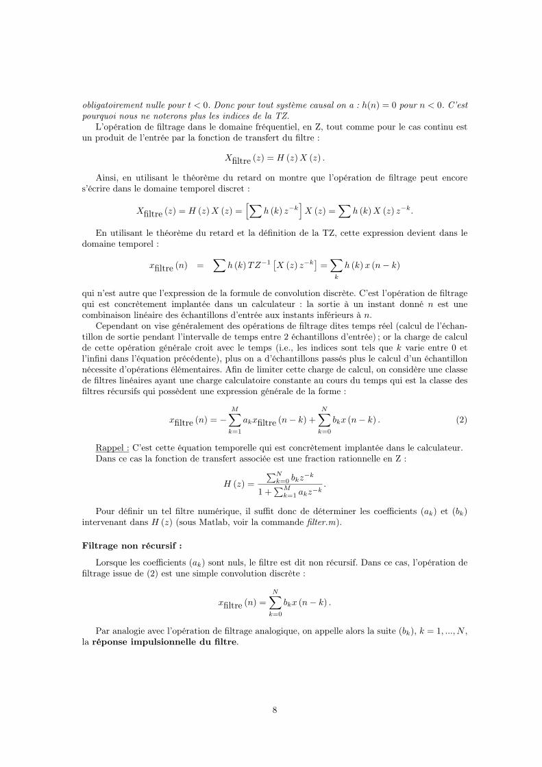
obligatoirement nulle pour t < 0. Donc pour tout système causal on a : h(n) = 0 pour n < 0. C’estpourquoi nous ne noterons plus les indices de la TZ.

L’opération de filtrage dans le domaine fréquentiel, en Z, tout comme pour le cas continu estun produit de l’entrée par la fonction de transfert du filtre :

Xfiltre (z) = H (z)X (z) .

Ainsi, en utilisant le théorème du retard on montre que l’opération de filtrage peut encores’écrire dans le domaine temporel discret :

Xfiltre (z) = H (z)X (z) =[∑

h (k) z−k]X (z) =

∑h (k)X (z) z−k.

En utilisant le théorème du retard et la définition de la TZ, cette expression devient dans ledomaine temporel :

xfiltre (n) =∑

h (k)TZ−1[X (z) z−k

]=

∑

k

h (k) x (n− k)

qui n’est autre que l’expression de la formule de convolution discrète. C’est l’opération de filtragequi est concrètement implantée dans un calculateur : la sortie à un instant donné n est unecombinaison linéaire des échantillons d’entrée aux instants inférieurs à n.

Cependant on vise généralement des opérations de filtrage dites temps réel (calcul de l’échan-tillon de sortie pendant l’intervalle de temps entre 2 échantillons d’entrée) ; or la charge de calculde cette opération générale croit avec le temps (i.e., les indices sont tels que k varie entre 0 etl’infini dans l’équation précédente), plus on a d’échantillons passés plus le calcul d’un échantillonnécessite d’opérations élémentaires. Afin de limiter cette charge de calcul, on considère une classede filtres linéaires ayant une charge calculatoire constante au cours du temps qui est la classe desfiltres récursifs qui possèdent une expression générale de la forme :

xfiltre (n) = −M∑

k=1

akxfiltre (n− k) +N∑

k=0

bkx (n− k) . (2)

Rappel : C’est cette équation temporelle qui est concrètement implantée dans le calculateur.Dans ce cas la fonction de transfert associée est une fraction rationnelle en Z :

H (z) =∑N

k=0 bkz−k

1 +∑M

k=1 akz−k.

Pour définir un tel filtre numérique, il suffit donc de déterminer les coefficients (ak) et (bk)intervenant dans H (z) (sous Matlab, voir la commande filter.m).

Filtrage non récursif :

Lorsque les coefficients (ak) sont nuls, le filtre est dit non récursif. Dans ce cas, l’opération defiltrage issue de (2) est une simple convolution discrète :

xfiltre (n) =N∑

k=0

bkx (n− k) .

Par analogie avec l’opération de filtrage analogique, on appelle alors la suite (bk), k = 1, ..., N ,la réponse impulsionnelle du filtre.

8

Synthèse d’un filtre non récursif par la méthode de la fenêtre :Il existe une méthode simple de synthèse d’un filtre numérique non récursif : la méthode de la

fenêtre consiste à calculer les coefficients (bk), k = 1, ..., N , du filtre souhaité en échantillonnantet tronquant la réponse impulsionnelle d’un filtre analogique idéal.

Par exemple, pour synthétiser un filtre passe-bas sur 2N +1 coefficients par cette méthode, onprocède de la manière suivante :

1. Expression du filtre analogique idéal :

H (f) = 1 pour f ∈ [−fc , fc] ,= 0 ailleurs.

2. Calcul de la réponse impulsionnelle du filtre analogique par transformée de Fourier inverse :h (t) = TF−1 {H (f)} = sin(2πfct)

πt .

3. Echantillonnage et troncature de h (t) : b0 = h(−N

fe

), ... , bN = h (0) , ... , b2N = h

(Nfe

).

9

2454 IEEE TRANSACTIONS ON SIGNAL PROCESSING, VOL. 49, NO. 11, NOVEMBER 2001

All-Purpose and Plug-In Power-Law Detectors forTransient Signals

Zhen Wang and Peter K. Willett, Senior Member, IEEE

Abstract—Recently, a power-law statistic operating on discreteFourier transform (DFT) data has emerged as a basis for a remark-ably robust detector of transient signals having unknown structure,location, and strength. In this paper, we offer a number of im-provements to Nuttall’s original power-law detector. Specifically,the power-law detector requires that its data be prenormalizedand spectrally white; a constant false-alarm rate (CFAR) and self-whitening version is developed and analyzed. Further, it is notedthat transient signals tend to be contiguous both in temporal andfrequency senses, and consequently, new power-law detectors inthe frequency and the wavelet domains are given. The resultingdetectors offer exceptional performance and are extremely easy toimplement. There are no parameters to tune. They may be consid-ered “plug-in” solutions to the transient detection problem and are“all-purpose” in that they make minimal assumptions on the struc-ture of the transient signal, save of some degree of agglomerationof energy in time and/or frequency.

Index Terms—Crack detection, nonlinear detection, signal de-tection, sonar detection.

I. INTRODUCTION AND CONTEXT

A. Background

I T IS often of considerable interest to identify short-durationnonstationarities in observed signals. Applications include

surveillance (e.g., [6]) in which an acoustic “transient” may in-dicate the presence of a threat, industrial monitoring (e.g., [16]),in which the number and severity of transients reflects machinehealth, and medicine (e.g., [2]). Naturally, the problem is com-paratively simple if the signal to be detected is known—the onlyuncertainty is the time of occurrence, but knowledge of the tran-sient is usually not available or dependable; of interest here isto detect transient signals with unknown form, location, andstrength. The hypothesis test is naturally composite, with anystructure open to challenge. Basically, the detector is tasked todetermine whether all observations belong to a known stationaryprobability distribution or whether they do not.

Now, if there were nothing whatever that could be assumedabout a transient signal, the detection task would be more or lesshopeless. There are, fortunately, two rather qualitative proper-ties that most transient signals possess. The first is the obvious

Manuscript received August 11, 2000; revised June 11, 2001. This workwas supported by the Naval Undersea Warfare Center under ContractN66604-99-1-5021 and by the Office of Naval Research under ContractN00014-98-1-0049. The associate editor coordinating the review of this paperand approving it for publication was Dr. Vikram Krishnamurthy.

The authors are with the Department of Electrical and Systems Engi-neering, University of Connecticut, Storrs, CT 06269-2157 USA (e-mail:[email protected]).

Publisher Item Identifier S 1053-587X(01)07771-6.

temporal contiguity: A transient signal is often couched as a lo-calized burst (or bursts) in time, although the duration of such aburst is unknown in most applications. The second is a tendencyfor most transient signals to be bandpass, that is, it is reasonableto expect most of a transient signal’s energy to be contained incontiguous frequency observations, although again, there is usu-ally little to be said aboutwhich frequencies.

To exploit only the former, and considering a transient eventas a two-sided change (at some unknown time, the observationsswitches from having pdf to having pdf , and at a later time,there is a return to ), Page’s test has been explored and foundto be quite useful [1], [5]. Very similar to this, Nuttall coucheda transient as a contiguous burst of bins in time, whereis known, and developed the “maximum” detector [13]. To ex-ploit only the latter, there are detectors that begin their workon frequency domain data (usually DFT bins). Via (maximumlikelihood) estimation of unknown signal parameters via the es-timation–maximization (EM) algorithm, a GLRT approach ispresented [21]. Of greatest interest here is Nuttall’s frequencydomain “power-law” detector [12], which will be introducedshortly. It is natural to use both kinds of contiguities, and for this,we have, for example, the Gaussian-mixture time-spectrogrammodel in [17] and the GLRT approaches arising from linear datatransformations (either time-frequency or time-scale) [3], [10],[11]. These transforms are directed toward signal representationand classification, trying to distinguish signals in the transformdomain.

In [23], an attempt was made to compare the performancesof a number of the above transient detection approaches on afairly wide variety of signals. Those using time contiguity alone(Page and “maximum”) were perhaps the sturdiest performersoverall but suffer from the need that certain parameters (signalstrength or length) be prespecified and that data be prewhitenedand prenormalized. Among the others, it was surprising thatthe most robust performance came from the simplest processor:Nuttall’s frequency-domain power-law statistic. It is a very gooddetector indeed, and in this paper, we show a number of waysto make it better still.

B. Nuttall’s Power-Law Statistic

There has been significant recent attention to Nuttall’spower-law detector [12], [14] due to its simple implementationand good performance. The test is based on the followingformulation. Under the signal-absent hypothesis ()—that thetime-domain data is complex white Gaussian noise—prepro-cessing by the magnitude-square DFT yields independent andidentically distributed (iid) exponential random variates. Under

1053–587X/01$10.00 © 2001 IEEE

WANG AND WILLETT: ALL-PURPOSE AND PLUG-IN POWER-LAW DETECTORS 2455

the signal-present hypothesis (), the DFT observations areno longer a homogeneous population of exponentials; Nuttall’sbasic assumption is that there aretwoexponential populations:

(1)

whereunit step function (unity for positive argument andzero otherwise);total number of FFT bins;magnitude-squared FFT bins;subset with size .

It is assumed that signal-present bins are uniformly dis-tributed among the FFT bins. Clearly, the precise probabilitylaw under depends on the transient signal itself, and thereis no particular reason to take (1) as fact. Nevertheless, there isconsiderable flexibility in (1) (mostly through the unspecified

), and the detector arising from it seems to work remarkablyfaithfully.

At any rate, dealing with the above model, Nuttall developedpower-law statistics [12] as an approximation to the optimal de-tector, and these have the form

(2)

where is an adjustable exponent. Notice that is the en-ergy detector that is optimal for , and , whichis the maximum-magnitude FFT bin, corresponds to the GLRTfor . Through extensive computational work, it has beenfound that the best compromise value foris 2.5 when infor-mation about is completely unavailable. Performance of thisparticular power-law detector is close to the best in this class ofdetectors. This independence from of the power-law is for-tunate.

The above power-law statistic requires prenormalized data,meaning that in the model must be available. As an extensionof power law to unknown noise level () cases, a constant false-alarm rate (CFAR) version was introduced [15]:

(3)

Clearly, is not affected by a scale factor.The statistic (2) does a yeoman’s job at detecting a wide va-

riety of block inhomogeneities, and it might be wondered whythis paper, intending to improve on it, has been written. The an-swer is three-fold, as follows.

1) The statistic (2) is designed with white noise of knownpower in mind; the fact is that the performance of (3) isdisappointing in white noise, whereas for colored noise,it has very little appeal at all. We thus extend (2) in anatural way. We estimate the noise power and normalizeon a bin-by-bin basis.

2) The statistic (2) is essentially optimal [12] given itsfrequency-domain model of (1) when there is nothingwhatever known about the signal-bearing set. How-ever, there is some tendency for real transient signalsto aggregate their energy in a band, meaning thathassome structure. The challenge is to take advantage of thistendency when it exists while avoiding any degradationin performance when it does not. We believe that we haveachieved this through the simple expedient of combiningcontiguous DFT bins.

3) Similar to the previous point, there is a definite tendencyfor real transient energy to be agglomerated in the timedomain, and a magnitude-square DFT essentially de-stroys any such information, but there is no reason why aDFT must be the preprocessing step. We investigate the(obvious) extension that a transform other than the DFTbe used.

Basically, the power-law detector is as yet neither a plug-in so-lution nor is it as good as it can be, and we offer some remedyhere.

The organization of the paper is as follows. In Section II,we first describe the detection problem for the colored noisecase and derive the associated CFAR (bin-by-bin normalized)power-law statistics. It is necessary to revisit the assumptionsby which the adjustable exponent[see (2)] is set, and we pro-pose a measure by which it should be chosen. In Section III,we propose extensions to exploit the contiguities of the tran-sient and thus develop new detectors both in the frequency andthe wavelet domain. It is unsatisfying to report on new detectorstructures without advice in threshold-setting, and in Section IV,we derive both the normal and saddlepoint approximations tothe signal-absent distributions, and naturally, we compare theseto simulation. Numerical comparisons between the detectors arepresented in Section V, and we offer concluding remarks in Sec-tion VI.

II. CFAR POWER-LAW DETECTOR

A. Problem Description and the CFAR Power-Law Statistic

The focus of this section is to detect transients buried incolored noise with unknown but stationary spectrum. Clearly,the CFAR Power-Law in [15, eq. (3)] is to be applied towhite noise and is not suitable here. As shown in Fig. 1, wewrite in a matrix a block of time domain observationsas , where is a column vector ofdimension whose th element is the time sample of index

.1 We immediately transform each column toits magnitude-squared frequency domain equivalent, andrecord . It is assumed that s

1To avoid possible contamination of this “reference” dataset by a transient’sincipient edge, it is best to ignore a “guard” of a few blocks of data prior to thatunder test.


Fig. 1. Data and preliminary processing. Original time-domain sequence is reorganized into blocks, and the column-wise magnitude-square FFT is performed.

are independent and that are known to benoise-only samples.2 The probability density function (pdf) ofthe th element of has the form

(4)

where are unknown but stationary.Note that the spectral behavior of a nonwhite background is

faithfully represented by the s. It is assumed that for theentire block of observation, theth frequency bin maintains amean background energy level for each of the blocks of

data. The first blocks provide some estimate of thislevel for each bin, and the goal is to test for some elevation inthese levels in thelast ( th) block. More specifically, the pdfof the under hypothesis follows a distribution identicalto . On the other hand, when signalenergy is present in theth bin, the density of becomes

(5)

where is the relative signal power per bin, that is, the overalltransient signal energy is , in which is the numberof signal-energy-bearing DFT bins. Overall, we have the model

2This assumption of independence is in practice only approximate. In whatfollows, for analysis, we use the assumption; our simulations are based on timedomain signals, and naturally, there is a truer representation of the dependencystructure.

(6)

where indicates the (unknown) subset with (unknown) sizeout of bins in which transient signal energy is to be found.

Note that although this model may appear to have a batch flavor,Fig. 1 indicates that transient signals are to be detected on-line,although block-by-block. Each block of data that tests negativefor transient signal energy joins the “window” of reference data,and hence, the least-recent block is removed to make room forit.

Following ideas similar to those frequently used in radarCFAR processing (e.g., [4]), we define the normalized magni-tude-squared frequency-domain observations as

(7)

and the new power-law statistic as

(8)

where is a real exponent. Clearly, is non-negative andis CFAR with respect to in the model of (6). Note thatnormalization schemes alternative to that in (7) could be chosen.For example, one could define in whichdenotes the element among whose rank is . It ispossible that such a scheme would offer improved robustness[4], but due to its similarity to (8), we do not discuss it here.

B. SNR Analysis to Choose

The best value for the powerin (8) is, in general, stronglydependent on , which is the number of signal-present bins.


Fig. 2. SNR analysis for Nuttall’s power-law statistics, with settings outputSNR = 24, N = 1024. (Left) Required input aggregate SNR for power-lawdetectors with different�. (Right) Input SNR-loss for different�.

This is not at all desirable since our goal is to find a detec-tion structure that does not depend on knowledge of such signalqualities. A clever contribution of [12] was the so-called “low-quality operating point analysis,” and it was found that

is a good choice over a wide range of. This analysis de-pended on explicit numerical calculation of performance, andalthough such analysis was possible for the exponential randomvariables in (2), and indeedwouldbe an option in (8), in some ofthe later statistics, it is not. Thus, here, we investigate a similarSNR analysis to suggest the best choice ofin (8) when in-formation about is unavailable. Signal-to-noise ratio (SNR),which is sometimes known as deflection [19], is not a com-pletely accurate determinant of detection performance but is awidely accepted alternative to exhaustive simulation or numer-ical integration. Given a statistic, the output SNR can be ex-pressed as

SNRVar

(9)

where denotes the conditional expectation, and varisthe conditional variance.

First, we exploit the SNR analysis to evaluatefor thepower-law statistics in [12]. The coincidence between ourresults and Nuttall’s suggests that the SNR analysis is areasonable method to choose the powerfor our new CFARstatistics. Based on statistic (2) and model (1), the associatedSNR can be shown to be

SNR (10)

where represents the Gamma function, anddenotes thetotal signal power in bins, which is also referred to as theinput aggregate SNR. Our purpose is to evaluate the requiredto yield fixed output for each . Example results fromSNR analysis for the power-law detectors with differentareshown in Fig. 2, where , and the output .

The right plot in Fig. 2 shows the input SNR-loss (ISL),which, with fixed output SNR and is defined as

ISL (11)

The ISL measures the input aggregate SNR that is sacrificedthrough use of a fixed exponent, as compared with the bestpossible exponent for that or the corresponding optimalstatistic. At any rate, it is immediately seen that the best valueof , achieving minimum average signal power per bin, changeswith and sweeps through all intermediate values. Whenis completely unknown, we obtain the best compromise valuefor via ISL ; from the figure, we findthat is that choice. The tendencies and results coincidewell with those obtained from the low-quality operation pointanalysis in [12]. Based on this, we claim, as in [12], that

is a good choice for a wide range of .Encouraged by the above, we apply the input SNR loss anal-

ysis to the detector in (8) to select. It is straightforward toderive the pdf of under and [8], and hence, we get,after some algebra, the result

SNR

(12)

where denotes the Beta function and represents thetotal signal power in bins, and blocks of previousDFT outputs are used for normalization. Example results forpower values 1, 1.5, 2, 2.5, and 3, are shown in Fig. 3, where

, output , and .3 It is clear that thereis no reason to explore . It is noted that the best value of,

3The larger the window sizeL, the better the normalization, but the moresusceptible the detector to a nonstationary background. The range6 � L � 32

is often discussed [4] and provides reasonable results; we chooseL = 10 hereas representative of that range.


Fig. 3. SNR for CFAR power-law statistics, with settings the outputSNR = 6,N = 256. Left figure: SNR for different�; right figure: the input SNR loss fordifferent�.

providing the minimum average signal power per bin with givenoutput SNR, changes with . Similar results will be observedby setting different and output SNR: is a goodchoice when information of is completely unknown, as ityields the least ISL over . Here, appears to be thebest choice.

III. CONTIGUITY-BASED DETECTORS

The knowledge of signal contiguity may aid in detection.Both time and frequency contiguities are exploited in both thewhite- (prenormalized) and colored-noise (self-normalizing)cases to improve the detection performance. For each case,the model and the corresponding statistics are described. Thedetector is actually a combination of a linear and a power-lawprocessor. Since precise contiguity information is unavailable,only the cases of two and three adjacent bins are studiedin this paper. Theoretical justification for these detectors isnot offered; however, they make intuitive sense, and theywork well. Further, although the exponentcould be chosendifferently for difference numbers of aggregated bins, we havefound that this is not a major concern, and we choosefromthe single-bin analyses of the previous section.

A. Contiguity-Based Detectors in the Frequency Domain

Just as with the power-law detectors in (2), only magnitude-squared FFT outputs are of concern here. Using the contiguitytendency in frequency, we modify Nuttall’s assumption that the

signal-present bins are uniformly distributed amongst therecord of to an assumption that there is a tendency that someof the signal-occupied bins are adjacent.

1) Prenormalized Case:New random variables are obtainedby combining two contiguous frequency bins. We define

. Assuming that the originalare independent and exponential (that is, that this is Nuttall’smodel in which data are assumed already to have been normal-ized and whitened), yields aGamma random variate.

We define our new power-law detectors

(13)

where and have same meanings as in (1). The statisticof (13) is easily extended as

(14)

to the case of three contiguous bins, and further extension isstraightforward. Bins are indexed modulo .

2) Self-Normalizing Case:A similar combiningprocess was adopted in the colored noise case by letting

. This combining approach results inmodified model and generates a new CFAR power-law detectorin the frequency domain as

(15)

The similar detector combines three contiguous bins.

B. Detectors in the Wavelet Domain

For time-domain observations, the DFT transforms a pure“time description” into a pure “frequency description” and,thus, clearly cannot take advantage of time contiguity. Thediscrete-time wavelet transform (DWT), which is an alternativeto the DFT, is much more local and finds a good compro-mise—a time–frequency description. Hence, detectors in thewavelet domain will benefit from both temporal and frequencycontiguity tendencies. The original work of Nuttall exploredonly the case the that preprocessing transformation was the


Fig. 4. Structure used inT andT to combine three adjacent bins in thewavelet space. Circles illustrate the definitionsU = C + C +

C .

DFT. The extension to other transforms, especially the wavelettransform, is both natural and (mostly) straightforward. Thereare many different choices of wavelet family, and each has itsproponents. However, only the simple Haar wavelet is exploreddue to its easy implementation, its orthogonality [20], and dueto the fact that a statistic that assumes as little as possible aboutthe transient to be detected is preferable.

1) Prenormalized Case:A derivation similar to that of Nut-tall results in the power-law detector in the wavelet domain, con-sidering that under a complex Gaussian noise assumption themagnitude-squared (orthonormal) DWT of the noise-only dataobeys an iid exponential distribution. That is, we have

(16)

where , is the th magnitude-squared DWTcoefficient of scale. The argument is that if time observations

follow an iid normal distribution, the corresponding DWTvector has identical pdf [22].

In the case of preprocessing by the DFT, it was argued thatthere is often a tendency for transient energy to crowd into con-tiguous frequency bins. There is similarly a tendency for tran-sient energy to be in nearby wavelet coefficients, as each refersto a scale that roughly matches that of the transient. As shownin Fig. 4, it is natural to adopt a tree structure in the WT case,and similar to of (14), we define

, and and invoke

(17)

Clearly, this detector is obtained by combining three local adja-cent bins in the wavelet space. It would be possible to combinetwo adjacent WT samples at the same scale, but it has proven tobe less effective than hoped, and we do not report it here.

2) Self-Normalizing Case:For each column time-do-main vector , let the s be the correspondingmagnitude-squared DWT coefficients for each scale index

, intra-block time index ,and block index . Similar to the frequencydomain, we have

(18)

where

We record , for, , and .

As in the frequency domain, this combining approach suggestsa new CFAR power-law detector

(19)

in the wavelet domain.

IV. PERFORMANCEANALYSIS

Since we are interested in transients with unknown structure,location, and strength, our performance analysis will concen-trate on the prediction of the threshold exceedance probabilityof the statistics under and, thus, to choose a proper thresholdto ensure a certain false alarm rate. We use the central limit the-orem (CLT) to get the normal approximation to the distributionof the statistics. However, since the normal approximation pro-vides poor approximation to deep tail probabilities, a procedureusing saddle-point approximation is also introduced. The per-formance of different statistics are also studied via numericalsimulation, where we set the total number of bins .

In the following analysis, we only consider detectors in thefrequency domain; analysis in the wavelet domain is preciselyequivalent, provided the transform is orthogonal.

A. Normal Approximation

• The Statistic :This is a summation over iid random variables and, thus,

must converge to a normal distribution by the central limittheorem [18]. Recall

(20)

which converges in law to a normal distribution by CLT,provided has finite second moment. As shownbefore, follows an iid distribution under

, and thus, we can compute the mean and variance ofas

Var

(21)

Having obtained this mean and variance, we have the fol-lowing result for : Under the assumption thats are


Fig. 5. Exceedance probability ofT with normal and saddlepoint approximations as a function of thresholdh. The right-truncated distribution is used in theimplementation of saddlepoint approximation. Here,N = 256, andT = 20 . The approximation results are compared with the simulation results represented bythe solid line.

iid for converges inlaw for large to Var .

• The Statistic :We cannot use the classical CLT directly here since the

detector is a summation over dependent, although iden-tical, random variables. However, in the following, weshow that the detectors converge to normal distributionsusing CLT after a rewriting of the statistics. Observe thatwe can rewrite as

(22)

where . Since are iidunder (we assume for convenience), we knowthat are iid. Thus, andconverge in law to

[recorded as ] via the CLT.Now, since , we know that follows

distribution , where

Var Var

is the correlation coefficient, which is affected by thepower law . If , we note that ; thus,clearly, ; if , our calculation reveals that

. For noninteger , a numerical method hasto be used to calculate. Fortunately, is close to unity;thus, to simplify, we set and thus approximateas convergent in law to .

• The Statistic :Approximating as in the analysis of , we

have that converges in law to , whereand

• The Statistic :For the detector as defined in (15), we know

follows the distribution. Again, assumingthat , we approximate as convergent in law


Fig. 6. Exceedance probability ofT with normal and saddlepoint approximation as a function of thresholdh. Here,N = 256, andL = 10. The right-truncateddistribution is used in the implementation of saddlepoint approximation, andT = 10 . The approximation results are compared with the simulation resultsrepresented by the solid line.

to , where andVar

Var

(23)

• The Statistic :As in the previous cases, and using

(24)

we approximate as convergent in law to.

B. Saddle-Point Approximation

The asymptotic normal distribution derived in the previoussection is easy to work with. However, as we will see later, the

normal approximation tends to estimate the tail probability rela-tively poorly. To obtain more accurate performance evaluation,here, we introduce the saddle-point approximation method thatcan be thought as a refinement of normal approximation via theindirect use of the Edgeworth expansion. Here, we state the finalresult, and omit the detailed development; see [7].

Let be iid with pdf , and letbe the corresponding Laplace transform

defined for . We define the sample meanaccording to [7, eq. (2.2.6)], and hence, the tail probability canbe approximated via the formula

(25)

where is the ML estimate of given , ,is the Esscher function ofth order, and is the normal-


Fig. 7. Example of signal and observation process for Figs. 8 and 9. The signal (left panel) is created by passing white Gaussian noise through an FIR filter witha passband0:4� < ! < 0:6� (the number of signal-present FFT bins is approximately 25). On the right, noise is added.

Fig. 8. Detection performances of new power-law statistics in the frequency and the wavelet domains in the prenormalized case. The exponent in each case is� = 2:5, and the transient duration isM = 20 samples; different panels refer to the number of frequency bins occupied by the signal.

ized cumulant. A detailed description of the above quantities isavailable in [7].4

C. Comparison of Approximations with Simulation

As mentioned earlier, the performance analysis in this sec-tion is focused on the exceedance probability of the statisticsunder the hypothesis. The results obtained using the normalapproximation and the saddlepoint approximation are shownand compared with results of numerical simulations based on

4In our case, forX obeying pdff(x), the moment generation function(MGF) does not exist. To resolve this, we simply truncateX to a valueT .

runs, for different statistics and different exponents, with.

For the white noise (prenormalized) case, we investigate thestatistics and that combine two and three contiguousFFT bins correspondingly and show the performance analysisof in Fig. 5. We can see that the normal approximation tendsto underestimate the tail probability, whereas the saddlepointapproach shows good prediction. It implies both that saddle-point approximation is an efficient method to analyze the per-formances of our statistics and and that setting the cor-relation coefficient as 1 is an acceptable approximation.


Fig. 9. Detection performances of new power-law statistics in the frequency and the wavelet domains in the prenormalized case. The exponent in each case is� = 2:5, and the transient duration isM = 50 samples; different panels refer to the number of frequency bins occupied by the signal.

For the colored noise (self-normalizing) case, we investigatethe statistics and and show the result of inFig. 6. According to our earlier SNR analysis, we are interestedin . Here, we set and to be consistentwith our later simulations. We can see that the normal approx-imation estimates the tail probability rather poorly, whereas thesaddlepoint approach shows much better prediction. It is noted,however, that even the saddlepoint approximation tends to mis-match the tail probability as grows large.

V. PERFORMANCECOMPARISON

Here , we apply the detectors developed in the previous sec-tions to numerical examples. For fixed , applyingthe thresholds obtained in Section IV, we compare probabilitiesof detection against aggregate SNR. TheaggregateSNR is thetotal signal energy divided by the total noise variance, meaningthat theper-sample(over the entire block and not just for thefuzzily-defined duration of the transient signal) SNR should bedivided by this number; for example, excellent performance isavailable at an aggregate SNR of 20 dB, and this translates to

4 dB per sample.Prenormalized Data:The detection performance of the im-

proved detectors in the frequency and the wavelet domains arecompared with the power law of [12] with exponent .Examples of the signal and noise are shown in Fig. 7 for anumber of signal-containing frequency bins . FromFig. 8, in which the time-domain transient signal is of length

samples, it is clear that combining two or three con-tiguous FFT or wavelet bins together does improve the detectionperformance over different SNRs. It is also noted that the de-tector based on the contiguity of wavelet bins shows ad-vantages over all others, and the explanation is presumably that

utilizes both temporal and frequency contiguity. However,in the case of a longer transient signal (see Fig. 9) for which thelength is samples, those transients that are more con-centrated in the frequency domain ( and ) arebest detected by the FFT-based statistic. This is further ex-plored in Fig. 10; here, contours of the probability of detectionare plotted on transient-length (vertical) and bandwidth (hori-zontal) axes for detectors and . It is clear that thewavelet-based detectors are more forgiving than those based onthe short-time frequency transformation, but that transients ofsufficiently narrow bandwidth and broad length are best servedin the latter domain.

Self-Normalizing Case:The results of detectors in the casethat self-normalization is required are shown in Fig. 11. Fromcomparison with Fig. 9 (the prenormalized case), it is clearthat the losses arising from the need to normalize are relativelyminor. It is also gratifying that the statistic is, in all thesecases, the best.

VI. SUMMARY

In [12], Nuttall derived and justified a new and easy-to-im-plement statistic for the detection of short-duration (transient)


(a) (b)

(c) (d)

Fig. 10. Probability of detection contours for (a)T , (b)T , (c)T , and (d)T . These are plotted versus transient lengthM and number of signal-occupantfrequency binsM .

signals: the sum of magnitude-square DFT outputs from a blockof time domain data, each raised to a power typically in therange of 2 to 3. This test has been found to be very effective in-deed.

The power-law detector is almost a plug-in transient detectorfor all purposes but not quite: Prewhitened and prenormalizeddata is required. We have thus extended the power-law detectorto be self-normalizing by raising to an exponent not the DFTdata directly but, instead, the power in each DFT bin relativeto the average power in previous DFTs. While Nuttall providedsome justification both for the exponentiation and exponent inthe original power-law test, their applicability in the self-nor-malizing case is not straightforward. Consequently, a mode ofanalysis (“input SNR loss”) has been proposed for the choiceof exponent. It is found that the optimal exponent is somewhatlower than in the original (prenormalized) power-law case.

At any rate, the self-normalizing solution works very nicely.All that is needed to have an all-purpose transient detector withsimple implementation is some means to set the threshold, andthis is provided via a saddle-point approximation.

Along the path to development of the improved CFARpower-law detector, it was noted that there is a tendency amongreal transient signals for energy to aggregate in nearby DFTbins (i.e., to be bandlimited to some degree). In their formu-lations, neither the original nor CFAR power-law detectorstake advantage of this, and consequently, a combined-binpower-law detector is proposed. In experiments, versions of

this are shown to offer significant improvement. These aremade self-normalizing, and a saddlepoint approximation forthreshold setting is provided. It was additionally noted thatthe power-law dogma of preprocessing via the DFT is opento the challenge, and indeed, a power-law processor operatingon (Haar) wavelets is developed, made self-normalizing,augmented to use combined bins (since transient signals mosttransient signals are aggregated not just in frequency but intime/scale as well), and accorded a saddlepoint approximationfor threshold setting.

Quite a few of the detectors have been developed and ana-lyzed in this paper. We note that beyond easy choices such aswindow size (for CFAR) or type (wavelet/DFT or agglomer-ating/single-bin) and guided selection of the exponent, there areno parameters to tune. We thus consider them to be “plug-in”transient detectors, and since they make minimal assumptionson the structure of the transient signal, save that it have somedegree of concentration of energy in time and/or frequency, weadvertise them as “all-purpose.” For reference, we give their tax-onomy in Table I.

Note that the choice of prenormalized versus self-normal-izing depends on the data, but in either case, our overall con-clusion is that although all of these tests work well, the com-bined/wavelet power-law detectors (if data are prenormalized,

, and if self-whitening and CFAR is necessary, ) areperhaps the finest of all. The statistics are compellingly simpleto use. Take a multiresolution decomposition using the Haar


Fig. 11. Detection performance of power-law detectors in the frequency and the wavelet domains for transient detection in colored noise. Here, the time-domaintransient length isM = 50, and the exponent used in all cases is� = 1:5.

TABLE ICATEGORIZATION OF VARIOUS TRANSIENT DETECTORSDISCUSSED IN THIS

PAPER. NUTTALL ’S CFAR POWER-LAW IS “PARTIALLY ” SELF-NORMALIZING

IN THAT IT IS COMPLETELY INSENSITIVE TOSCALE BUT HAS NO MEANS TO

DEAL WITH NONWHITE DATA

basis, normalize the magnitude-square by previous values ateach scale (in the self-whitening case only), combine the resultin groups of three according to Fig. 4, exponentiate (to a power2.5 if prenormalized and to the power 1.5 if normalized), andsum. The resulting statistic can be relied on to detect quite a widerange of transient signals below (often considerably below)3dB on a sample-by-sample basis.

REFERENCES

[1] M. Basseville and I. Nikiforov, Detection of AbruptChanges. Englewood Cliffs, NJ: Prentice-Hall, 1993.

[2] A. Bianchi, L. Mainardi, and E. Petrucci, “Time-variant power spectrumanalysis for the detection of transient episodes in HRV signal,”IEEETrans. Biomed. Eng., vol. 40, pp. 136–144, Feb. 1993.

[3] B. Friedlander and B. Porat, “Performance analysis of transient detectorsbased on a class of linear data transforms,”IEEE Trans. Inform. Theory,vol. 38, pp. 665–673, Mar. 1992.

[4] P. Gandhi and S. Kassam, “Analysis of CFAR processors in nonhomo-geneous background,”IEEE Trans. Aerosp. Electron. Syst., vol. 24, pp.427–444, July 1988.

[5] C. Han, “Transient signal detection and Page’s test,” Ph.D. dissertation,Univ. Conn., Storrs, 1996.

[6] T. Hemminger and Y.-H. Pao, “Detection and classification of under-water acoustic transients using neural networks,”IEEE Trans. NeuralNetworks, vol. 4, pp. 712–718, Sept. 1994.

[7] J. Jensen,Saddlepoint Approximation. Oxford, U.K.: Clarendon,1995.

[8] N. Johnson, S. Kotz, and N. Balakrishman,Continuous Univariate Dis-tribution, 2nd ed. New York: Wiley, 1995, vol. 2.

[9] S. Kassam,Signal Detection in Non-Gaussian Noise. London, U.K.:Dowden & Culver, 1988, pp. 31–46.

[10] N. Lee and S. Schwartz, “Robust transient signal detection using theoversampled Gabor representation,”IEEE Trans. Signal Processing, vol.43, pp. 1498–1502, June 1995.

[11] S. Marco and J. Weiss, “Improved transient signal detection usinga wavepacket-based detector with an extended translation-invariantwavelet transform,” IEEE Trans. Signal Processing, vol. 45, pp.841–850, Apr. 1997.

[12] A. Nuttall, “Detection performance of power-law processors forrandom signals of unknown location, structure, extent, and strength,”NUWC-NPT Tech. Rep., Newport, RI, 10 751, Sept. 1994.


[13] , “Detection capacity of linear-and-power processor for randomburst signals of unknown location,” NUWC-NPT Tech. Rep., Newport,RI, 10 822, Aug. 1997.

[14] , “Near-optimum detection performance of power-law processorsfor random signals of unknown location, structure, extent, and arbitrarystrengths,” NUWC-NPT Tech. Rep., Newport, RI, 11 123, Apr. 1996.

[15] , “Performance of power-law processors with normalization forrandom signals of unknown structure,” NUWC-NPT Tech. Rep., New-port, RI, 10 760, May 1997.

[16] Y. Ohya, Y. Takahashi, and M. Murata, “Acoustic emission from a porce-lain body during cooling,”J. Amer. Ceramic Soc., pp. 445–448, Feb.1999.

[17] L. Perlovsky, “A model-based neural network for transient signal pro-cessing,”Neural Networks, vol. 7, no. 3, pp. 565–572, 1994.

[18] V. Petrov, Limit Theorems of Probability Theory. Oxford, U.K.:Clarendon, 1995, p. 113.

[19] H. V. Poor,An Introduction to Signal Detection and Estimation, 2nded. New York: Springer-Verlag, 1994.

[20] G. Strang and T. Nguyen,Wavelets and Filter Banks. Wellesley, MA:Wellesley-Cambridge, 1996.

[21] R. Streit and P. Willett, “Detection of random transient signals via hy-perparameter estimation,”IEEE Trans. Signal Processing, vol. 47, pp.1823–1834, July 1999.

[22] B. Vidakovic, Statistical Modeling by Wavelets. New York: Wiley,1999, p. 169.

[23] Z. Wang and P. Willett, “A performance study of some transient de-tectors,”IEEE Trans. Signal Processing, vol. 48, pp. 2682–2685, Sept.2000.

Zhen Wang was born in China on January 17,1974. She received the B.S. degree with honors fromTsinghua University, Beijing, China, in 1996 and theM.Sc. degree from the University of Connecticut,Storrs, in 2000, both in electrical engineering. She iscurrently pursuing the Ph.D. degree at the Universityof Connecticut.

Her present research interests include the detectiontheory and signal processing.

Peter K. Willett (SM’97) received the B.A.Sc.degree in 1982 from the the University of Toronto,Tornto, ON, Canada, and the Ph.D. degree in 1986from Princeton University, Princeton, NJ.

He has been a Professor at the University of Con-necticut, Storrs, since 1986. His interests are gener-ally in the areas of detection theory and signal pro-cessing.

Dr. Willett is an Associate Editor for boththe IEEE TRANSACTIONS ON AEROSPACE AND

ELECTRONICSYSTEMSand the IEEE TRANSACTIONS

ON SYSTEMS, MAN, AND CYBERNETICS.

projet de traitement du signal : détection de transitoires sur des

Documents