proofs for tra c safety - university of liverpoolslk/drafts/linpro15.pdf · foremost, i thank...

Carl von Ossietzky Universitat OldenburgFakultat II – Informatik, Wirtschafts- und Rechtswissenschaften

Department fur Informatik

Proofs for Traffic Safety

Combining Diagrams and Logic

Dissertation zur Erlangung des Grades eines Doktors der Naturwissenschaften

vorgelegt von

Sven Linker

Tag der Disputation: 20.02.2015

Gutachter:

Prof. Dr. Ernst-Rudiger OlderogProf. Dr. Michael Reichhardt Hansen

Abstract

Due to the increasing interest in autonomously driving cars, safety issues of such systemsare of utmost importance. Safety in this sense is primarily the absence of collisions, whichis inherently a spatial property. Within computer science, typical models of cars includespecifications of their behaviour, where the space a car needs for operating safely is afunction of time. This complicates proofs of safety properties tremendously.

In this thesis, we present methods to separate reasoning on space from the dynamicalbehaviour of cars. To that end, we define an abstract model with an emphasis onspatial transformations of the situation on the road. Based on this model, we developtwo formalisms: We give the definitions of a modal logic suited to reason about safetyproperties of arbitrarily many cars. Furthermore, we present a diagrammatic languageto ease the specification of such properties. We formally prove that no collisions arisebetween cars obeying a small set of requirements.

i

Zusammenfassung

Durch das steigende Interesse an autonomen Fahrzeugen gewinnt deren Sicherheit immerstarker an Bedeutung. Hierbei ist Sicherheit gleichbedeutend mit Kollisionsfreiheit, einegrundsatzlich raumliche Eigenschaft. Fahrzeugmodelle in der Informatik beinhaltenSpezifikationen des dynamischen Verhaltens, so dass der zum sicheren Betrieb notigeRaum abhangig von der Zeit ist. Dies erschwert Sicherheitsbeweise enorm.

In dieser Arbeit stellen wir Methoden vor, um Schlussfolgerungen uber den Raum vomFahrzeugverhalten abzutrennen. Hierzu definieren wir ein abstraktes Modell mit demSchwerpunkt auf den raumlichen Veranderungen der Straßensituation. Darauf aufbauendentwickeln wir zwei Formalismen: Wir definieren eine Modallogik, mit der Aussagen uberdie Sicherheit von beliebig vielen Fahrzeugen bewiesen werden konnen. Weiterhin stellenwir Diagramme zur einfacheren Spezifikation solcher Eigenschaften vor. Wir beweisendie Kollisionsfreiheit zwischen Fahrzeugen, die wenige Anforderungen erfullen.

iii

Acknowledgements

I could not have finished my thesis without the help of many different people. First andforemost, I thank Ernst-Rudiger Olderog for supporting me throughout my time at theUniversity of Oldenburg, both during my undergraduate studies as well as during mytime as a Ph.D. student. Furthermore, I thank Michael Reichhardt Hansen for being myexternal examiner and for the helpful feedback he gave during my visit in Lyngby.

While I wrote the text of this document, Manuel Gieseking, Martin Hilscher and MaikeSchwammberger were willing to suffer and proofread different chapters. I am especiallyindebted to Manuel Gieseking, who checked many of the proofs. All of the remainingerrors are due to myself.

The pleasant atmosphere in the working group “Correct System Design” was stronglyshaped by all of my former and current colleagues along the different groups workingon theoretical computer science in Oldenburg: Marion Bramkamp, Bjorn Engelmann,Evgeny Erofeev, Johannes Faber, Hans Fleischhack, Nils-Erik Flick, Sibylle Froschle,Manuel Gieseking, Andrea Goken, Martin Hilscher, Soren Jeserich, Stephanie Kemper,Heinrich Ody, Christoph Peuser, Jan-David Quesel, Hendrik Radke, Uli Schlachter, MaikeSchwammberger, Tim Strazny, Mani Swaminathan, Patrick Uven, Ira Wempe and ElkeWilkeit. Thank you very much.

The beginning of my Ph.D. studies was influenced immensely by my fellows in thegraduate school “TrustSoft”: Amna Asif, Ahmad El Maamoun, Kinga Kiss-Iakab, HenrikLipskoch, Nils Mullner, Felix Oppermann, Hendrik Radke and Astrid Rakow. Manythanks to all of you for the instructive meetings, the great trips to Dagstuhl and the nicediscussions. It was an honour to meet you. Especially, I would like to thank Ira Wempefor being a great coordinator of the graduate school and for listening to all the problemswe had.

Of course, there are people who supported me outside of academia. I would like tothank Christian Bruns, Markus Dahlke, Karsten Fritzsch, Manuel Gieseking, Niels Hapke,Markus Lohmeyer, Andreas Schafer, Alexander Skobel and Tim Strazny for their constantsupport and time, for relaxed discussions, for great vacation trips, and in general for beingfriends. Special thanks go to my current and former flatmates Holger Brettschneider,Marcus Dreßler, Sebastian Richter and in particular Cathrin Vogel for helping me duringthe hard times of the last years, as well as for being part of the fun activities we hadtogether. Thank you, I owe you very much.

v

Contents

1 Introduction 11.1 Contributions . . . . . . . . . . . . . . . . . . . . . . . . . . . . . . . . . . 31.2 Structure of this Thesis . . . . . . . . . . . . . . . . . . . . . . . . . . . . 4

2 Preliminaries 52.1 Mathematical Notations . . . . . . . . . . . . . . . . . . . . . . . . . . . . 52.2 Temporal Logic and Interval Logic . . . . . . . . . . . . . . . . . . . . . . 72.3 Labelled Natural Deduction . . . . . . . . . . . . . . . . . . . . . . . . . . 82.4 Graph Rewriting . . . . . . . . . . . . . . . . . . . . . . . . . . . . . . . . 11

3 Spatial Model of Traffic 193.1 Abstract Road . . . . . . . . . . . . . . . . . . . . . . . . . . . . . . . . . 203.2 Bounded Visibility . . . . . . . . . . . . . . . . . . . . . . . . . . . . . . . 253.3 Sensor Models . . . . . . . . . . . . . . . . . . . . . . . . . . . . . . . . . . 273.4 Related Work . . . . . . . . . . . . . . . . . . . . . . . . . . . . . . . . . . 28

4 Modal Logic for Freeway Traffic 314.1 Syntax and Semantics . . . . . . . . . . . . . . . . . . . . . . . . . . . . . 314.2 Proof System . . . . . . . . . . . . . . . . . . . . . . . . . . . . . . . . . . 364.3 Undecidability of Spatial MLSL . . . . . . . . . . . . . . . . . . . . . . . . 594.4 Related Work . . . . . . . . . . . . . . . . . . . . . . . . . . . . . . . . . . 65

5 Visual Logic for Freeway Traffic 695.1 Concrete Syntax . . . . . . . . . . . . . . . . . . . . . . . . . . . . . . . . 705.2 Conveniences . . . . . . . . . . . . . . . . . . . . . . . . . . . . . . . . . . 765.3 Formalising Sanity . . . . . . . . . . . . . . . . . . . . . . . . . . . . . . . 775.4 Abstract Syntax . . . . . . . . . . . . . . . . . . . . . . . . . . . . . . . . 805.5 Semantics . . . . . . . . . . . . . . . . . . . . . . . . . . . . . . . . . . . . 975.6 Decidability of Spatial Traffic Diagrams . . . . . . . . . . . . . . . . . . . 1045.7 Related Work . . . . . . . . . . . . . . . . . . . . . . . . . . . . . . . . . . 107

6 Combining Text and Diagrams 1116.1 Comparison of Expressivity . . . . . . . . . . . . . . . . . . . . . . . . . . 1116.2 Verification Framework . . . . . . . . . . . . . . . . . . . . . . . . . . . . . 121

vii

Contents

6.3 Related Work . . . . . . . . . . . . . . . . . . . . . . . . . . . . . . . . . . 122

7 Case study 1257.1 Controller Specification . . . . . . . . . . . . . . . . . . . . . . . . . . . . 1267.2 Safety Proof . . . . . . . . . . . . . . . . . . . . . . . . . . . . . . . . . . . 1277.3 Refining the Specification . . . . . . . . . . . . . . . . . . . . . . . . . . . 133

8 Conclusion 1378.1 Summary . . . . . . . . . . . . . . . . . . . . . . . . . . . . . . . . . . . . 1378.2 Future Work . . . . . . . . . . . . . . . . . . . . . . . . . . . . . . . . . . 138

Bibliography 141

Index 150Symbol Index . . . . . . . . . . . . . . . . . . . . . . . . . . . . . . . . . . . . . 150Subject Index . . . . . . . . . . . . . . . . . . . . . . . . . . . . . . . . . . . . . 152

viii

List of Figures

1.1 Decomposing Reasoning about Traffic . . . . . . . . . . . . . . . . . . . . 2

2.1 Semantics of the chop modality . . . . . . . . . . . . . . . . . . . . . . . . 7

2.2 Example of a Graph Rewriting Rule . . . . . . . . . . . . . . . . . . . . . 13

2.3 The graph G . . . . . . . . . . . . . . . . . . . . . . . . . . . . . . . . . . 13

2.4 Possible Results of Applying r once to G . . . . . . . . . . . . . . . . . . . 14

2.5 The Hyperedge Replacement System R . . . . . . . . . . . . . . . . . . . 16

2.6 Example of a Graph Rewriting Rule with an Application Condition . . . . 16

3.1 Situation on a Freeway at a Single Point in Time . . . . . . . . . . . . . . 20

5.1 Spatial Traffic Diagram . . . . . . . . . . . . . . . . . . . . . . . . . . . . 70

5.2 Example of a Topological Sequence . . . . . . . . . . . . . . . . . . . . . . 72

5.3 Example of a Lane Sequence . . . . . . . . . . . . . . . . . . . . . . . . . 73

5.4 Example of Distance Arrows . . . . . . . . . . . . . . . . . . . . . . . . . . 73

5.5 Omission of Notation for Conjunction . . . . . . . . . . . . . . . . . . . . 76

5.6 Ambiguities with Sequences . . . . . . . . . . . . . . . . . . . . . . . . . . 76

5.7 Sanity Conditions as Diagrams (I) . . . . . . . . . . . . . . . . . . . . . . 78

5.7 Sanity Conditions as Diagrams (II) . . . . . . . . . . . . . . . . . . . . . . 79

5.7 Sanity Conditions as Diagrams (III) . . . . . . . . . . . . . . . . . . . . . 79

5.8 Connectedness of Cars . . . . . . . . . . . . . . . . . . . . . . . . . . . . . 80

5.9 Alignment of Cars . . . . . . . . . . . . . . . . . . . . . . . . . . . . . . . 80

5.10 Abstract Syntax of Fig. 5.1 . . . . . . . . . . . . . . . . . . . . . . . . . . 83

5.11 Concrete and Abstract Syntax of a Diagram with Duration Arrows . . . 84

5.12 Rule Sets RLS , RSEP , RCH and ROCC : Lane/Topological Sequences . . . 86

5.13 Rule Sets RBL , RLA, RT and RI : Structure of Spatial Diagrams . . . . . 87

5.14 Hyperedge Replacement Grammar for the Definition of Paths . . . . . . . 89

5.15 Rule RsingCS : Distance Arrow from Left to Right of a Topological Situation 89

5.16 Different Possibilities for Distance Arrows . . . . . . . . . . . . . . . . . . 90

5.17 Application Condition for Distance Arrows between Different Lanes . . . 90

5.18 Rules R1CS and R2

CS : Distance Arrow between Cars . . . . . . . . . . . . . 91


CS : Distance Arrow attached to Left of Target . . . . . 92


CS : Distance Arrow attached to Right of Source . . . . . 93

ix

List of Figures

5.21 Rule R7CS : Distance Arrow on the Same Lane from Right to Left . . . . . 94

5.22 Rule R8CS : Distance Arrow on Different Lanes from Right to Left . . . . . 94

5.23 Rule Sets RS , RBD , RL and RAT : Structure of Traffic Diagrams . . . . . 955.24 Semantics for Logical Connectives . . . . . . . . . . . . . . . . . . . . . . 985.25 Semantics of Sequences . . . . . . . . . . . . . . . . . . . . . . . . . . . . 995.26 Semantics of Layers . . . . . . . . . . . . . . . . . . . . . . . . . . . . . . 1005.27 Semantics of Lane Sequences . . . . . . . . . . . . . . . . . . . . . . . . . 1015.28 Semantics of Topological Sequences . . . . . . . . . . . . . . . . . . . . . . 1025.29 Semantics of Distance Arrows . . . . . . . . . . . . . . . . . . . . . . . . . 1035.30 Concrete and Abstract Syntax of an Example Diagram . . . . . . . . . . . 1045.31 Example of a Spatial Diagram . . . . . . . . . . . . . . . . . . . . . . . . . 1045.32 Problematic Example for Decidability . . . . . . . . . . . . . . . . . . . . 1065.33 A Time-Distance Diagram for Railways . . . . . . . . . . . . . . . . . . . 1075.34 A Time-Space Diagram . . . . . . . . . . . . . . . . . . . . . . . . . . . . 108

6.1 Schema of a Spatial Diagram . . . . . . . . . . . . . . . . . . . . . . . . . 1126.2 Example for the Metric Transformation . . . . . . . . . . . . . . . . . . . 1136.3 New Rule R5

BD: Formulas . . . . . . . . . . . . . . . . . . . . . . . . . . . 121

6.4 Example of a Combination of EMLSL and Traffic Diagrams . . . . . . . . 1226.5 Proving Safety with EMLSL and Traffic Diagrams . . . . . . . . . . . . . 122

7.1 Positive Conditions for the Creation of Reservations . . . . . . . . . . . . 1347.2 Withdrawal of Reservations . . . . . . . . . . . . . . . . . . . . . . . . . . 1357.3 Distance Controller Preserving Free Space in Front of Cars . . . . . . . . 136

x

List of Tables

4.1 Instructions for Counter c1 of a Two-Counter Machine . . . . . . . . . . . 59

5.1 Diagrammatic Elements of Traffic Diagrams . . . . . . . . . . . . . . . . . 715.2 Terminal Types of the Abstract Syntax . . . . . . . . . . . . . . . . . . . 82

xi

1Introduction

The amount of individual traffic is still on the rise, and will probably continue to do soin the near future. The reduction of accidents in spite of the increase of traffic density istherefore a main goal of much research involving the development of cars. Advanced driverassistance systems support the human driver by supplying different kinds of information.They may, e.g., display warnings whenever the current velocity is higher than allowed.Furthermore, they often provide visual means to inform the driver whether changinglanes is possible in a safe way. However, the human element within traffic is still a sourcefor unsafe situations, e.g., when drivers overestimate the capabilities of their car, or areexhausted due to a long drive.

To further ensure safety, the development of automated cars capable of driving au-tonomously has been and is still of strong interest. The PATH project [Hsu+94] was oneof the pioneering projects constructing and analysing the behaviour of fully autonomouscars. The results of this project led to the identification of several manoeuvres the con-trollers of such cars have to support. Furthermore, it was possible to derive constraintsensuring safety, i.e., the prevention of collisions. Several safe controllers for cars havebeen presented, e.g., by Lygeros et al. [LGS98] and Jula et al. [JKI99] within this project.

In all of these works, the dominant role in both the specification of the controllers, aswell as in proving their safety, is played by the car dynamics. Safety in these approachesis always defined as the avoidance of collisions, which is an inherently spatial property. Byusing differential equations, the positions and braking distances of cars are only derivedelements of the model, which tremendously increases the complexity of proofs.

Intuitively, safety of traffic is only dependent on the local environment of each car.Consider for example two cars C and D. If the distance between both is very large, e.g.,100 kilometres, the behaviour of one should not concern the safety of the other. Insteadof mimicking such a property on a syntactic level, it should be inherent in the modeldefinition itself to avoid clutter in specifications.

We want to specifically address the problem of safety on freeways with these ideas in

1

1 Introduction

Spatial Abstraction

Dynamics

Focus ofthis thesis

Interface

Figure 1.1: Decomposing Reasoning about Traffic

mind. To that end, we want to reason locally with an emphasis on the spatial propertiesof traffic. For that, we want to examine how spatial properties and locality restrictionscan be incorporated into a model of traffic as first-class citizens, and in what way sucha model eases proofs of spatial safety predicates. That is, we decompose the reasoningprocess into two levels as shown in Fig. 1.1. On the upper level, the topology of space andits evolution over time is the main focus of reasoning. That is, the model should reflectwhich parts of the freeway are occupied by cars and how these parts change while thecars drive along their current lane, and when they change lanes. On the lower level, thedynamics specify the concrete trajectories, how the cars perform these changes. Hencethere has to be an exchange of information between both levels, as indicated by thearrows in Fig. 1.1. On the one hand, the abstraction has to get information about thesize of the occupied space from the dynamics. On the other hand, mode changes withinthe layer of dynamics can be initiated by the upper level. Now assume that we havespecified a protocol for the behaviour of cars on the spatial abstraction and shown thatit prohibits collisions. Then we only have to prove that the dynamic layer respects theconstraints for the behaviour implied by the upper level, and that it provides the spatialabstraction with the correct information for our protocol to work.

For formal reasoning purposes, the use of logics and especially modal logics has a longstanding tradition within computer science. Logic provides a good trade-off between beingsuccinct and precise. Furthermore, such a logical approach benefits from meta-theoreticalresearch, e.g., the development of proof systems or methods to decide satisfiability offormulas algorithmically. Proof systems allow the user to reason only on formulas and todisregard the concrete semantic structures, as long as the main properties of the semanticsare captured within axioms and proof rules. They may also be implemented withininteractive or automated theorem provers, thus providing the user with the guarantee tocreate a correct proof. Tools checking satisfiability may be used for example to decidewhether a formal syntactic proof should be attempted. For this, the desired propertyis negated and then checked for satisfiability. If the algorithm decides that the negatedproperty can be satisfied, all attempts to formally prove the validity of the property arefutile. Due to these advantages, many approaches to prove safety (or other interestingproperties) of software and hardware devices make extensive use of logical methods andformulas in general.

2

1.1 Contributions

However, within engineering practice, formulas and mathematical descriptions lackthis acceptance. There, visual languages play a more prominent role. For example,for software engineering, the Unified Modelling Language (UML) [RJB04; UML12] iswell-established. It incorporates, e.g., Message Sequence Charts (MSCs) [ITU96], whichare used to define the communication between several independent objects, and timingdiagrams [UML12], which are able to express timing relations between events occurring inchip-designs. Similarly, depictions of electronic circuits are used widely to communicateabout specifications and implementations of computing devices. But most of thesediagrammatic languages lack a precise semantics. For example, within MSCs, it is notalways clear whether a diagram states a possible or a necessary course of events.

Still, several diagrammatic languages have been provided with a formal semantics.While general mathematical properties may be captured by formal Euler- and Venn-Diagrams [Shi95; AB96], only few diagrams extensively used in computer science wereformalised in this way. MSCs have been enhanced by a mathematical semantics in thedefinition of Life Sequence Charts [DH01], which also extend MSCs with methods todistinguish universal and existential sequences. Schlor examined timing diagrams formally[Sch01]. In the context of real-time systems, Kleuker presented a visual specificationlanguage called Constraint Diagrams [Kle00].

1.1 Contributions

With these considerations at hand, the contributions of this work are the following. Wedefine a model of freeway traffic that clearly distinguishes space from the dynamicalbehaviour of cars. This model also emphasises the local environment of a single car, andby that is a suitable model for the remainder of this thesis. An explicit formalisation ofthe sensors provided by the cars on the freeway completes the model.

Using this model as the semantics, we present the extended multi-lane spatial logic(EMLSL) to reason locally about spatial properties of freeway traffic. While the logiccannot express concrete properties of the dynamics, it is able to distinguish differentdiscrete changes in the space on the road. Within the logic, both qualitative aspects, i.e.,the topological situations on the freeway, as well as quantitative aspects, e.g., the lengthof free space ahead of a car or the number of lanes between two different cars, can bereferred to. As a first step towards tool assistance, we present a formal proof system inthe style of natural deduction and derive several useful rules within this system.

To further ease the use of our approach, we define a formal diagrammatic languagecalled Traffic Diagrams, which uses the abstract model of traffic as a semantics. Similar tothe logic, the diagrams incorporate methods to reason about the existence of transitionsand to measure distances between cars. For a clearly defined syntax, we do not onlydefine the visual elements used within the diagrams, but give a formal syntactic definitionin terms of hypergraphs. This formal syntax may be used to take advantage of alreadyexisting methods and tool support for diagram parsing.

We compare the expressiveness of Traffic Diagrams and EMLSL. As it will turn out,the diagrams are not as expressive as the logic. To that end, we present a translation

3

1 Introduction

of diagrams into equivalent formulas. Furthermore, we discuss how the diagrams andformulas may be used in conjunction to exploit their respective advantages.

Finally, we apply all of these formalisms to specify a small set of requirements restrictingthe possible behaviour of cars. In addition, we define a safety predicate, which is expressingthe absence of collisions. We then formally prove the safety predicate to be invariantalong all possible transition sequences of the abstract model of traffic with the help ofthe deductive system for the logic.

1.2 Structure of this Thesis

After this introduction, we present definitions and conventions that we will use throughoutthis thesis in Chap. 2. Chapter 3 is devoted to the development of the abstract modelof traffic that we use as a semantics. In Chap. 4, we define the logic EMLSL and proveits undecidability. Furthermore, this chapter contains the proof system together withseveral derived rules. Chapter 5 contains the definitions needed for the visual languageof Traffic Diagrams. We present both the concrete and abstract syntax as well as aformal semantics. In addition, the chapter includes formalisations of certain propertiesthe abstract model possesses and a sketch for a decidable subset of diagrams. Thecombination of EMLSL and Traffic Diagrams is explored in Chap. 6, in which we alsocompare the expressiveness of both approaches. Chapter 7 presents the application ofthe proof system and the diagrams to a case study, defining the required constraints forsafe behaviour within freeway traffic. Finally, Chap. 8 concludes the thesis.

4

2Preliminaries

Contents

2.1 Mathematical Notations . . . . . . . . . . . . . . . . . . . . . . 5

2.2 Temporal Logic and Interval Logic . . . . . . . . . . . . . . . . 7

2.3 Labelled Natural Deduction . . . . . . . . . . . . . . . . . . . . 8

2.4 Graph Rewriting . . . . . . . . . . . . . . . . . . . . . . . . . . . 11

In this chapter, we present most of the work this thesis is based upon. We first give thebasic notations used throughout the following work in Sect. 2.1. In Sect. 2.2 and Sect. 2.3we recall the preliminaries for the first part of the thesis, i.e., the concepts and definitionsof different interval logics and labelled natural deduction, respectively. Following that,we present graph rewriting in Sect. 2.4, which plays a crucial role for the syntax of thediagrams in this thesis.

2.1 Mathematical Notations

In this section, we introduce general mathematical notation. While the notation itselffollows mathematical standards, we include it for reference purposes.

Sets For a set S, the powerset of S, i.e., the set of all subsets of S, is denoted by P(S).We use the usual notations ∪, ∩ and \ for the union, intersection and difference of sets.To denote the disjoint union, we use the symbol ]. The Cartesian product of the sets Sand T , i.e., the set of all ordered tuples (s, t) with elements taken from the sets S and T ,is denoted by S × T .

We use the standard notations for the different sets of numbers, i.e., N for the positive

5

2 Preliminaries

integers and R for the real numbers. The positive reals are denoted by

R+ = x ∈ R | x ≥ 0 .

In this thesis, we will make extensive use of intervals over both the positive integers andthe real numbers. We denote closed borders of intervals with brackets and open borderswith parenthesis. Furthermore, we also allow for infinity as a right border. For example,a typical interval we will use is the interval of all positive reals [0,∞) (= R+). We denotethe set of all real-valued intervals, i.e., intervals over the reals with I. Sometimes, wewant to use variables as the borders of an interval. We will use the notation IVar to referto the set of all variable intervals, i.e., where the borders are either variables or realnumbers. Observe that I ⊂ IVar.

Let i ∈ I with the borders a and b, i.e., i = [a, b], i = (a, b], i = [a, b) or i = (a, b). Wecall the set i \ a, b the interior of i, denoted by I(i).

Relations and Functions If S and T are sets, R ⊆ S × T is a relation between S andT . The domain of R is the set of all elements of S which are related to an element of T .Similarly, the range of R is the set of all elements of T which are related to elements of S.If both the domain and range of R are subsets of the same set S, i.e., R ⊆ S × S, thenwe call R a relation on S. We denote the reflexive and transitive closure of a relation Ron a set S by R∗.

A function is a relation f ⊆ S × T , which is functional and total, i.e.,

(s, t1) ∈ f and (s, t2) ∈ f implies t1 = t2 (Functionality),for all s ∈ S there is a t ∈ T such that (s, t) ∈ f (Totality) .

We denote the function f itself by f : S → T and its elements (s, t) ∈ f by f(s) = t. If arelation f is only functional, but not total, we call f a partial function. If f : S → T is a(partial or total) function, the image of S′ ⊆ S is given by

f(S′) = t ∈ T | ∃s ∈ S′ • f(s) = t .

Injectivity of a function means, that each element of the range is related to exactly oneelement of the function’s domain, i.e.,

(s1, t) ∈ f and (s2, t) ∈ f implies s1 = s2 (Injectivity) .

If f is injective, we denote the preimage of an element t of T by f−1(t) = s, wheref(s) = t. To denote the function modification, we use notation taken from the Zspecification language [Smi00]. That is, for the function f , we use f ⊕x 7→ y to denotethe function which coincides with f except for f(x) = y. For two functions f : S → Tand g : T → U , the function g f : S → U is the composition of g and f , given by(g f)(x) = g(f(x)) as long as both f(x) and g(f(x)) are defined.

A sequence is a function f with either the natural numbers or a finite subset of them asits domain. We will often denote a sequence f with the domain 0, . . . , n by 〈c0, . . . , cn〉,

6

2.2 Temporal Logic and Interval Logic

where f(i) = ci for all i ∈ 0, . . . , n. The elements ci are the values of the sequence. IfS is a set, we use the notation S∗ for the set of all finite sequences with values in S. Itwill be clear from the context whether we use this notation for sequences or the reflexivetransitive closure of a relation. If we want to apply the function g to all elements of thesequence 〈c0, . . . , cn〉, we also write g(〈c0, . . . , cn〉) for the sequence 〈g(c0), . . . , g(cn)〉.

2.2 Temporal Logic and Interval Logic

Reasoning about temporal changes by means of logical formulas has a long history. Thefirst approach to use a temporal logic, i.e., a modal logic to formalise properties of time isdue to Prior [Pri57]. He introduced the modalities G and F with the intended meaningof “it will always be the case” and “it will be the case”, respectively, as well as H and P ,which stand for “it has always been the case” and “it was the case”, respectively. Prioranalysed the modalities with respect to a totally ordered linear time scale, i.e., for twotime points x and y, either x was later than y, or y was later than x, or both stood forthe same time point. Such models are models of linear time. For the specification andverification of computational systems, linear temporal logic (LTL), as presented by Pnueli[Pnu77], is a typical formalism inspired by Prior’s work. In computer science, logics withsemantics of branching time are also of strong importance, with the most famous examplebeing computational tree logic (CTL), introduced by Emerson and Clarke [EC82]. Insteadof interpreting time as a linearly ordered domain, they consider a tree of states, each ofwhich may possess an arbitrary number of children. CTL then provides operators toreason about paths originating at the current node, and about the occurrence of stateson these paths.

A different approach to describe temporal properties is due to both Moszkowski[Mos85] and Halpern and Shoham [HS91]. Halpern and Shoham introduced a modal logic,subsequently called HS, where the modalities correspond to Allen’s interval relations[All83]. The main application of HS and its extensions lies in the field of artificialintelligence, where the different relations describe the knowledge about time (or otherdomains) an agent may possess. Moszkowski introduced interval temporal logic (ITL) tospecify and verify hardware specifications. The models of both of these approaches arebased on (usually finite) intervals. In the following, we will concentrate on ITL.

Within ITL, intervals can be divided into their subintervals, to describe, e.g., thebeginning or the end of the intervals. For this purpose, Moszkowski introduced the chopmodality a . An interval [a, b] satisfies a formula ϕaψ, if and only if there is a pointc such that a ≤ c ≤ b, where [a, c] satisfies ϕ and [c, b] satisfies ψ. A depiction of thisinterpretation is given in Fig. 2.1. The syntax of ITL is basically first-order logic with

ϕ ψ

ϕaψ

a c b

Figure 2.1: Semantics of the chop modality

7

2 Preliminaries

the addition of the chop-modality:

ϕ ::= ⊥ | θ1 = θ2 | ϕ1 → ϕ2 | ∀x • ϕ1 | ϕ1aϕ2 ,

where θ1 and θ2 are terms over a given signature. ITL distinguishes between rigidand flexible terms. The values of the former are given globally by a valuation of thevariables, while the semantics of the latter may change with respect to the interval underconsideration. A typical example of a flexible variable would be the length of an interval.We will not go further into the details of the semantics of ITL. Both ITL itself as well asextensions like the Duration Calculus [ZHR91] or Neighbourhood Logic [BRZ99] havebeen proven valuable for the specification and verification of real-time systems.

2.3 Labelled Natural Deduction

In his PhD thesis, Gentzen [Gen35] developed the calculus of natural deduction to presentan alternative to axiom-based proof systems. Natural deduction is based on a set ofproof rules and (temporary) assumptions, to give a tighter connection between the waymathematicians “naturally” prove theorems and the formal proof system. To that end,the system comprises an introduction and an elimination rule for each operator (with thepossible exception of the falsum proposition ⊥). A derivation within natural deductionconsists of a tree, where the root is the theorem to prove and the leaves are the assumptionsused within the proof. The branches from the root to the assumptions are determinedby the structure of the proof rules. Each rule may possess application conditions, whichrestrict the form of the assumptions in the branches above the application of this rule.These conditions can ensure, e.g., freshness of variables or terms for rules concerningthe quantors in first-order logic. A main feature of natural deduction is that rulesmay eliminate assumptions from the derivation. The underlying idea of this methodis that the information of the eliminated assumption is already comprised within theconclusion of the rule. For example, if we can derive the truth of a formula ψ fromthe assumption that the formula ϕ holds, then ϕ→ ψ reflects exactly this information.Hence, we can eliminate ϕ from the set of assumptions and disregard it in the rest of thederivation. This mechanism is a formal counterpart to the informal mathematical strategyto use temporary assumptions within a proof. For example, within case distinctions wetemporarily assume the truth of each case and derive our desired conclusion independently.Within natural deduction, we would use the elimination rule for the disjunction operatorfor such a purpose. A proof in natural deduction is a derivation, where all assumptionshave been eliminated. In derivations, we will mark eliminated assumptions by enclosingthem in square brackets. To identify the application of the rule which was the reason whythis particular assumption was eliminated, we add a unique index to both the assumptionand the application of the rule within the tree.

While this approach is well-suited for classical logic and intuitionistic logic, other non-classical logics impose problems. For example, to define rules covering general modalities,application conditions for the rules have to constrain the set of all assumptions, not onlythe set of assumptions involved in the formula to prove [Pra06].

8

2.3 Labelled Natural Deduction

A way to preserve the underlying structure of natural deduction is to augment theformulas in the proof with information about the semantics. This leads to systems oflabelled natural deduction (LND) [Sim94; BMV98; Vig00]. In labelled natural deduction,one of the basic entities are labelled formulas w : ϕ, where ϕ is a formula of the logic andw is a name of a world. Intuitively, the labelled formula w : ϕ means that the formula ϕholds at world w. The reachability relation between the worlds R is defined by relationalformulas of the form wRv, where w and v are names for worlds. The formula wRvexpresses that v is reachable from w. By adding suitable rules concerning relationalformulas, different types of reachability relations may be defined. For example, theaddition of the following rules defines, that R is both reflexive and transitive, and henceis the underlying reachability relation of all S4-frames.

wRwwRv vRu

wRu

For an operator , we denote the elimination rule of by E. Similarly, we use thenotation I for the introduction rule of . The rules concerning classical propositionaland first-order logic operators are similar to standard natural deduction rules. In thepresentation of the rules, we will denote the syntactical substitution of x by a term tin the formula φ by φ[x 7→ t]. Following the notations of Basin et al.[BMV98], we usethe name ⊥E for reductio ad absurdum. Note that this rule is the only one concerningfalsum.

w : ϕ→ ψ w : ϕ → Ew : ψ

[w : ϕ]

...w : ψ → I

w : ϕ→ ψ

[w : ¬ϕ]

...v : ⊥ ⊥Ew : ϕ

w : ϕ ∧ ψ ∧Ew : ϕ

w : ϕ ∧ ψ ∧Ew : ψ

w : ϕ w : ψ ∧Iw : ϕ ∧ ψ

w : ∀x • ϕ ∀Ew : ϕ[x 7→ t]

w : ϕ[x 7→ t]∀I

w : ∀x • ϕ

The application condition for ∀I is that t may not occur in any assumption w : ϕ[x 7→ t]depends on. The rule ⊥E allows for a contradiction to be propagated along the reachableworlds. That is, we take ⊥ to be a global contradiction [Vig00]. A main advantageof the labelling approach is that the behaviour and intention of the modalities can becaptured by rules which only use the typical mechanisms of natural deduction, i.e.,application conditions and elimination of assumptions. Furthermore, the introductionand elimination rules for a box modality can be defined without any further knowledgeabout the properties of the reachability relation R:

w : ϕ wRvE v : ϕ

[wRv]

...v : ϕIw : ϕ

9

2 Preliminaries

The application condition of the introduction rule I is that v is different from w and maynot occur free in any assumption v : ϕ depends on, except for wRv. The box eliminationrule states that whenever ϕ holds on w, and v is reachable from w, then ϕ holds on v.The introduction rule states that if we can deduce the truth of ϕ on v, where the onlyassumption on v is that it is reachable from w, then we know that ϕ holds on all worldsreachable from w. Hence ϕ holds on w. This is exactly the intended semantics of abox-like modality.

We will often use the rules for the derived operators, i.e., ∨, ¬, ↔, ∃ and diamond-likemodalities. To spare the reader the search of these rules in the literature, we include therules for these operators.

w : ¬ϕ w : ϕ ¬Ew : ⊥

[w : ϕ]

...w : ⊥ ¬Iw : ¬ϕ

w : ϕ ∨ ψ

[w : ϕ]

...v : χ

[w : ψ]

...v : χ ∨Ev : χ

w : ϕ ∨Iw : ϕ ∨ ψ

w : ψ ∨Iw : ϕ ∨ ψ

[w : ϕ]

...w : ψ

[w : ψ]

...w : ϕ ↔ I

w : ϕ↔ ψ

w : ϕ w : ϕ↔ ψ ↔ Ew : ψ

w : ψ w : ϕ↔ ψ ↔ Ew : ϕ

w : ϕ[x 7→ t]∃I

w : ∃x • ϕw : ∃x • ϕ

[w : ϕ]

...v : χ ∃Ev : χ

v : ϕ wRv ♦Iw : ♦ϕ

w : ♦ϕ

[v : ϕ] [wRv]

...u : χ ♦Eu : χ

The application condition for ∃E is that x appears free neither in any assumption v : χdepends on (except for w : ϕ) nor in v : χ itself. Similarly, in the rule ♦E, v has to bedifferent from both u and w and may not appear in any assumption u : χ depends on,except for wRv. Usually, the rules for the quantifiers have to assert the existence ofthe terms t substituted for the variable x. In this thesis, we will assume constant andinfinite domains of quantification, and therefore the existence of the terms is guaranteed,allowing us to omit these additional assumptions.

LND has been transferred to interval logics by Rasmussen [Ras01; Ras02]. In hiswork, the reachability relation is ternary and labelled formulas are of the form [a, b] : ϕ,where [a, b] is an interval on which ϕ is true. Rasmussen used a generalised interval logiccalled signed interval logic (SIL), where intervals may also have a “negative length”, i.e.,

10

2.4 Graph Rewriting

he allows for intervals [a, b], where a > b. He defined rules capturing, e.g., the singledecomposition property of intervals [Dut95], and the behaviour of the chop-modalities,and achieved a sound and complete proof system.

For a well-defined proof system, Rasmussen also needed to express whether a termor formula is rigid and whether a formula does not contain a chop-modality, i.e., ischop-free. Since these properties are both of syntactic nature, predicates for rigidity andfor chop-freeness can be straightforwardly defined. Furthermore, Rasmussen extended theproof system for SIL with suitable axioms and rules to embrace, for example, DurationCalculus or Neighbourhood logic.

2.4 Graph Rewriting

In this section we present the basic ideas of graph rewriting based on hypergraphs. Eventhough we present the formal definitions, we will mostly focus on the intuitive notions.However, we will give references to complete formalisations of the approaches describedin this section.

The first thing needed for the definition of a graph rewriting system is a notion ofgraphs. In this thesis, we will use typed hypergraphs, a generalisation of graphs.

Definition 2.1 (Typed Hypergraph). Let T be a set of types and O a set of labels.A typed hypergraph G = (V, E , τ, θ, l) over T and O consists of a set of vertices V,hyperedges (or edges for short) E, an attachment function τ : E → V∗, a type functionθ : E → T and a labelling function l : E → O. In contrast to edges in usual graphs, ahyperedge e may connect an arbitrary number of vertices, we say it visits the nodes viaits tentacles. We use typed hypergraphs, i.e., the type θ(e) of an edge e determines thenumber of vertices e must be visiting. Hence for all edges e of the same type, the sequenceτ(e) is of the same length. We denote the set of all typed hypergraphs by the set G.

Even though, the attachment function of a hypergraph returns sequences, we willintroduce a more mnemonic notation to refer to the elements of the sequence. Since thelength of the sequence for all edges of one type is equal, we will not speak of the indexof a node within the sequence, but refer to it by a short string, e.g., i or at. This willbe used to have a more intuitive way to describe graphs. If we refer to different graphsG and H, we will sometimes use the notation VG and VH to denote the set of verticesof the corresponding graph, and similarly for the other elements of the graphs. For thevisualisations of typed hypergraphs, we use small black circles to denote the vertices andgrey rectangles with rounded corners to denote the hyperedges, where the type of theedge is inscribed in the rectangle. The tentacles of the edges are given by the labelledconnections between the edges and the vertices. Labels are presented as rectangles, whichare connected with the edge they label by a dashed line. For the definition of graphrewriting systems, we now have to introduce graph homomorphisms.

Definition 2.2 (Graph Homomorphisms). Let G and H be two typed hypergraphs. Thetwo functions fV : VG → VH and fE : EG → EH form a graph homomorphism, if they are

11

2 Preliminaries

edge preserving and compatible with the attachment function, as well as the typing andlabelling functions. That is, for all edges e ∈ EG such that τG(e) = 〈v0, . . . , vn〉 we have

τH(fE(e)) = 〈fV(v0), . . . , fV(vn)〉 ,θH(fE(e)) = θG(e) ,

lH(fE(e)) = lG(e) .

The pair fV and fE will simply be abbreviated by f : G→ H and by abuse of notation, wewill use the name f to denote both functions. In general, we will only consider injectivegraph homomorphmisms, i.e., both fV and fE have to be injective functions.

Graph rewriting systems [Roz97] are a generalisation of formal grammars. Whereformal grammars replace occurrences of strings with other strings, graph rewriting systemsallow for the replacement of graphs with other, possibly more complex graphs. Hencesuch rewriting systems allow for the creation of a language of graphs. Even though graphrewriting systems are often defined in terms of category theory, we give a definitionwithin set theory, following the presentation of Baldan et al.[BKK03]. First, we have todefine what a graph rewriting rule consists of.

Definition 2.3 (Rewriting Rule). A graph rewriting rule (or production) p = 〈L,R, α〉is defined by its left-hand side (LHS) L and its right-hand side (RHS) R, as well as theinjective function α : VL → VR, which we will usually indicate by labelling correspondingvertices of L and R by natural numbers.

A rule p is applicable to a graph G, if there exists an injective graph homomorphismm : L→ G, a match of L in G. Given a match m of L in G, the application of p to Gresults in a new graph H, given by

VH = VG ] (VR \ α(VL))

EH = (EG \m(EL)) ] ERand with the function m : VR → VH given by m(v) = m(α−1(v)) if v ∈ α(VL) andm(v) = v otherwise, the attachment, type and labelling function are defined as

e ∈ EG \m(EL)⇒ τH(e) = τG(e), θH(e) = θG(e), lH(e) = lG(e)

e ∈ ER ⇒ τH(e) = m(τR(e)), θH(e) = θR(e), lH(e) = lR(e)

We denote the application of a rule p to the graph G resulting in H by G Z⇒p H.

Intuitively, the application of a rule p to a graph G consists of replacing an occurrenceof a subgraph F of G that matches the LHS with the RHS, where vertices are identifiedby the function α.

Example 2.1. Consider the rule r shown in Fig. 2.2. The injective function of r isgiven by the nodes labelled 1 and 2. The labels determine, which nodes are identifiedin the LHS and RHS during the application of the rule. So let us consider the graph Gshown in Fig. 2.3. We can apply r at three different occurrences of the LHS of r to G.This yields the three graphs shown in Fig. 2.4. Of course, r could be applied to thesegraphs again, until no edge of the type S occurs in the results anymore.

12

2.4 Graph Rewriting

S

1

2

s

t

→1

2H

u v

Figure 2.2: Example of a Graph Rewriting Rule

aS

S

c

d

S

e

s

t

s

t

s t

Figure 2.3: The graph G

A graph rewriting system (or graph transformation system) consists basically of aset of rewriting rules. In addition, it contains the axiom, denoting the graph where allderivations of the system have to start at.

Definition 2.4 (Graph Rewriting System). A graph rewriting system G = (T, S, P )consists of a set of types T , an axiom S, i.e., a typed hypergraph over T , and a set ofrewriting rules P , where all graphs occurring in P are typed hypergraphs over T . If His the result of an arbitrary sequence of applications of rules within G to the graph G,we write G Z⇒∗G H, or simply G Z⇒∗ H, if G is clear from the context. We say that thereexists a derivation of H from G.

Unfortunately, this approach is not expressive enough for our purposes. We needthe possibility to constrain the application of rules more than just through the mereoccurrence of a subgraph. For that, we employ nested conditions [HP09] or rather theirextension HR∗ conditions [HR10; Rad13].

Intuitively, nested conditions allow not only for the statement whether a certainsubgraph matching the left-hand side exists, but also for further conditions on theenvironment of this match. For example, it is possible to state that a certain othersubgraph shall not exist, for a rule to be applicable. HR∗ conditions extend this notionby allowing for variables within the conditions, which have to be instantiated by graphsthat are created by a hyperedge replacement system. A hyperedge replacement system isa graph rewriting system, where the LHS of each rule may only refer to one hyperedge atonce. For example, the rule r given above is such a rule.

13

2 Preliminaries

aS

H

c

d

S

e

c′

u

v

s

t

s t

(a) Replacing the Left Edge

aH

S

c

d

S

e

d′

s

t

s

t

v

u

(b) Replacing the Middle Edge

aS

S

c

d

H

e

e′s

t

v

u

s t

(c) Replacing the Right Edge

Figure 2.4: Possible Results of Applying r once to G

Definition 2.5 (Graph Substitution). Let X be a set of edge types and R a hyperedgereplacement system. A graph substitution induced by R is a function σ : X → G wherex Z⇒∗R σ(x) for all x ∈ X. We denote the application of a substitution σ to the graph G,i.e., the simultaneous replacement of all occurrences of edges in the domain of σ withinG by Gσ.

The main syntactic element of HR∗ conditions is ∃(h, c), where h : P → C is a graphhomomorphism and c a graph condition. For a given graph G, this notation shall describethe existence of a subgraph Cσ within G, i.e., a subgraph described by the applicationof a suitable graph substitution σ to C. The subgraph Cσ then has to further satisfythe condition c. This construction allows us, e.g., to express the existence of a pathof arbitrary length within G. With the condition c, additional constraints on the path(or even the environment of the path) can be defined. The other crucial element ofthe conditions is ∃(P w C, c), where P and C are graphs and c is a graph condition.This notation gives us the ability to “cut” certain elements from graphs used within theconditions and only refer to the elements of C subsequently (respectively, the elements ofCσ for a substitution σ). With this construction, we can circumvent the injectivity ofthe underlying graph morphisms.

The full syntax of HR∗ conditions is given by the following definition.

Definition 2.6 (HR∗ Graph Condition). Let R be a hyperedge replacement system and Gbe a hypergraph possibly containing hyperedges that can be replaced by R. For a hypergraphP , the set of HR∗ conditions over P is given inductively as follows:

1. > is a HR∗ condition over P .

2. Let P be a subgraph of C, where h : P → C is the inclusion of P in C and let c bea HR∗ condition over C, then ∃(h, c) is a HR∗ condition over P .

3. Let C be a graph and c a HR∗ condition over C, then ∃(P w C, c) is a HR∗ conditionover P .

14

2.4 Graph Rewriting

4. Let c and c′ be HR∗ conditions over P , then both ¬c and c ∧ c′ are HR∗ conditionsover P .

If the domain of the inclusion in the second case of the definition is obvious from thecontext, we may omit it. That is, instead of ∃(P → C, c), we would write ∃(C, c).

We now define the semantics of a HR∗ condition based on graph homomorphisms,to have a clearly defined notion of satisfaction. In the following definition, we use thenotation cσ for a condition c and a substitution σ, do denote the recursive application ofσ to all graphs occurring within c.

Definition 2.7 (Semantics of HR∗ Conditions). Let g : P → G be a graph homomorphism. Then the satisfaction of c by g, denoted by g |= c is defined as follows.

1. g satisfies >.

2. g satisfies ∃(h, c) iff h : P → C and there is a substitution σ which replaces allvariable edges of C and a graph homomorphism q : Cσ → G with q hσ = g1 suchthat q satisfies cσ

3. g satisfies ∃(P w C, c) iff there is a substitution σ such that Cσ ⊆ P and a graphhomomorphism f : Cσ → G satisfying cσ such that g restricted to Cσ coincides withf , i.e., g|Cσ = f .

4. g satisfies ¬c iff g does not satisfy c.

5. g satisfies c ∧ c′ iff g satisfies c and g satisfies c′.

If g has the domain ∅, i.e., g : ∅ → G and g satisfies the HR∗ condition c, we also saythat G satisfies c.

We define the abbreviations for the missing Boolean connectives and universal quan-tification as usual. Furthermore, we will omit any conditions of the form >, e.g., insteadof ∃(C,>), we only write ∃(C). Observe that the substitution σ in the semantics ofthe conditions replaces each occurrence of a variable edge by the same graph. This willbe unfortunate for our main purpose, when we want to state the existence of several,structurally different paths defined by the same hyperedge replacement system. However,Radke showed that simultaneous replacement of variables by substitutions and replace-ment of variables with different graphs (which are still derivable by the replacementsystem) are equally expressive [Rad13]2. We chose to present the semantics based onsubstitutions, since they require less notational overhead, but will use the conditions as ifwe defined the semantics based on replacement.

1hσ is the graph homomorphism which coincides with h for all elements of P , but has Cσ as its range.Observe that all elements of C have a unique counterpart within Cσ, and hence hσ is uniquelydetermined.

2The main idea of the proof that substitution is as expressive as replacement is to create a new variabletype for each occurrence of a variable within a condition. The replacement rules for these new typesare then defined to be similar to the original variable type. The other direction is more involved.

15

2 Preliminaries

If we want to formally add a HR∗ condition as an application condition to a ruler = 〈L,R, α〉, we use the following approach. We start with the condition ∃(L w I, c0),where I is the graph induced by the restriction of α to only the nodes of L, i.e., it consistsof a discrete graph. Then, within the condition c0, we can constrain possible connectionsbetween these nodes, e.g., claim the existence of a path. This extra step is needed, sincewe want to “reuse” the elements of the left-hand side within the condition, which isnormally prevented by the injectivity of all homomorphisms involved.

Definition 2.8 (Application of a Rule with a HR∗ condition). Let r = 〈L,R, α〉 be arewriting rule enhanced with the HR∗ condition c over L. Then r is applicable to thegraph G, if there exists a match m : L→ G and m |= c. The application of r to G is thendefined as in Definition 2.3.

Visually, we use an abbreviation. If we want to add an application condition ∃(L w I, c)to a rule r = 〈L,R, α〉, we depict c to the left of the LHS of r and separate c from r witha white triangle.

P

1

2

s

t

→ S

1

P

2s

t s

tS

1

2

s

t

Figure 2.5: The Hyperedge Replacement System R

Example 2.2. As an example, consider the hyperedge replacement system R, consistingof the rules shown in Fig. 2.5. It replaces the hyperedge P by a path of S edges of anarbitrary length greater than zero. Using R, we can define a HR∗ condition to restrict theapplications of the rule r of Fig. 2.2. Consider the modification of r as shown in Fig. 2.6.

S

1

2

s

t

¬∃

2

P

1s

t

→1

2H

u v

Figure 2.6: Example of a Graph Rewriting Rule with an Application Condition

The application condition states that the rule may only be applied, whenever thereis no path of S edges starting at the node labelled 2. That is, the second applicationof r as shown in Fig. 2.3 would not be possible anymore. Observe that it prohibits the

16

2.4 Graph Rewriting

unlabelled node and the node with the label 1 to be identified due to the injectivity of thehomomorphisms involved.

If there are several rules with the same left-hand side, we use a notation similar to theextended Backus-Naur form to achieve a compact depiction of such rules (see, e.g., therules defining the hyperedge replacement system R in Fig. 2.5). Then, if a rule has morethan one alternative, we use the following convention to easily refer to each of these.

Convention 2.1. If there is more than one alternative for a left-hand side of rules, wewill add superscripts 1, 2, 3, . . . to the names of the rules to refer to the first, second,third, . . . alternative of the right-hand sides of the rule.

17

3Spatial Model of Traffic

Contents

3.1 Abstract Road . . . . . . . . . . . . . . . . . . . . . . . . . . . . 20

3.2 Bounded Visibility . . . . . . . . . . . . . . . . . . . . . . . . . . 25

3.3 Sensor Models . . . . . . . . . . . . . . . . . . . . . . . . . . . . 27

3.4 Related Work . . . . . . . . . . . . . . . . . . . . . . . . . . . . . 28

In this chapter we define the model we use to reason about traffic situations. Here weconcentrate on a model of freeway traffic [Hil+11], i.e., we do not consider cars driving inopposing directions or intersections of streets. A main property we want to maintain inthe model is its independence of the dynamics of the cars. Such a model will enable usto decompose reasoning about traffic safety into two parts. On the upper level, spatialarguments allow to show traffic safety properties, e.g., disjointness of space needed foremergency braking manoeuvres. Then, on the lower level, controllers only need to complywith the spatial constraints of the model, and safety for the overall system, i.e., thefreeway, will follow. Still, to keep the model descriptive, we will give a simple type ofdynamics, but will also give the required (but still very weak) restrictions on possible cardynamics. As long as the actual car dynamics adhere to the spatial constraints impliedby our model, the properties proven with the techniques presented in this thesis will hold,even with more concrete and expressive dynamics.

Figure 3.1 shows an exemplary situation on a freeway. For each car, we have bothindicated its physical size (the small polygon) as well as its braking distance, i.e., thedistance it needs in case of an emergency braking to come to a complete standstill. Wewill call the sum of these the safety envelope of the car. Note that already this picturecontains an important abstraction: car A has been depicted as driving on two lanes atthe same time. This notion shall indicate that A is presently engaged in a lane-changemanoeuvre. Hence we already abstracted from the concrete physical position of A. The

19

3 Spatial Model of Traffic

E

E

C

A

AB

physicalsize

braking distance safety envelope

Figure 3.1: Situation on a Freeway at a Single Point in Time

dotted instance of car E denotes that E has currently set its turn signals to indicate itsdesire to change to the lane to its right. In the next section, we will formalise situationssimilar to this figure and describe the possible behaviour of cars. The dashed rectangleshall denote the finite part of space that the car E perceives at the moment, as impliedby the sensors implemented in E.

The model of traffic is divided into different sections. First, we will define how all carsmay behave on the street, i.e., we give an abstraction of the freeway and what actionscars may perform on this abstraction. Afterwards, we will restrict this model to thepart a single car may perceive at a point in time. Then, we will make use of an abstractfunction ΩE , which defines the behaviour of the sensors of a car E. Finally, we are ableto define how each car perceives different cars on the freeway: simply as their physicalsizes, or with additional knowledge of their braking distances.

3.1 Abstract Road

We allow for an infinite (but countable) number of cars on the street. Each car isassociated with a unique identifier, which may be thought of, e.g., as its license plate.The set of such car identifiers is I. We will usually denote elements of I with uppercaseletters, e.g., C,D ∈ I. The road itself comprises an arbitrary but fixed number N > 1 oflanes, which are given by the set L = 1, . . . , N ⊂ N. We will make use of addition andthe total order on natural numbers, subsequently.

For simplicity, we assume each lane to be of infinite extension, so that we do not haveto consider start- or endpoints of the road. Hence we take the extension of the freewayto be the set of real numbers R. Throughout this thesis, we chose to use continuous time,i.e., the time domain T is fixed to be T = R+.

As shown in Fig. 3.1, we distinguish between two spatial properties for each car. First,each car reserves a certain amount of space on the freeway. This space is determinedby the actual position on the freeway and the physical size of the car. Furthermore,depending on the model of the cars sensors, it may include its braking distance. A typicalsafety property would include that the reservations of all cars are disjoint during the

20

3.1 Abstract Road

whole observation.

In contrast to reservations, the space claimed by a car may be thought of as a test, ora virtual image of the car, to check whether a lane change manoeuvre is possible. Hencea claim models that a car sets its turn signals to indicate an upcoming lane change.

In Fig. 3.1, the reservations are drawn solid, while the claim of E is given by a dottedpolygon. We will use this convention throughout this thesis.

Definition 3.1 (Traffic Snapshot). Let L be a fixed, finite set of lanes and I a countablyinfinite set of car identifiers. A structure T S = (res, clm, pos, spd , acc), is a trafficsnapshot, where res, clm, pos, spd and acc are functions

• res : I→ P(L) such that res(C) is the set of lanes the car C reserves,

• clm : I→ P(L) such that clm(C) is the set of lanes the car C claims,

• pos : I→ R such that pos(C) is the position of the car C along the lanes,

• spd : I→ R such that spd(C) is the current speed of the car C,

• acc : I→ R such that acc(C) is the current acceleration of the car C.

This model of the freeway is still very broad. To make a tighter connection betweenreal freeways and this abstract notion, we restrict the model in several ways. First, werequire all cars to reserve at least one, and at most two lanes. A car reserving two lanes atonce is assumed to be in the process of changing from one lane to the other. Furthermore,a car may only set its turn signals, if it is not already engaging a lane-change. Finally, acar may only try to change to a lane adjacent to its current lane. These requirements arecaptured in the following sanity conditions of traffic snapshots.

Definition 3.2 (Sanity Conditions). A traffic snapshot T S is sane, if the followingconditions hold for all C ∈ I.

1. res(C) ∩ clm(C) = ∅

2. 1 ≤ |res(C)| ≤ 2

3. 0 ≤ |clm(C)| ≤ 1

4. 1 ≤ |res(C)|+ |clm(C)| ≤ 2

5. |res(C)| = 2 implies ∃n ∈ L • res(C) = n, n+ 1

6. clm(C) 6= ∅ implies ∃n ∈ L • res(C) ∪ clm(C) = n, n+ 1

We denote the set of all sane traffic snapshots by TS.

Example 3.1. We formalise Fig. 3.1 as a traffic snapshot T S = (res, clm, pos, spd , acc).We will only present the subsets of the functions for the cars visible in the figure. Assuming

21


that the set of lanes is L = 1, 2, 3, where 1 denotes the lower lane and 3 the upper one,the functions defining the reservations and claims of T S are given by

res(A) = 1, 2 res(B) = 1 res(C) = 3 res(E) = 2clm(A) = ∅ clm(B) = ∅ clm(C) = ∅ clm(E) = 1

For the function pos, we chose arbitrary real values which still satisfy the relative positionsof the cars in the figure. Similarly, we instantiate the function spd such that the safetyenvelopes of the cars could match the figure. For example, since the safety envelope ofB is larger than the safety envelope of C, B has to drive with a higher velocity. Forsimplicity, we assume that all cars are driving with constant velocity at the moment, i.e.,for all cars, the function acc returns zero.

pos(A) = 28 pos(B) = 3.5 pos(C) = 2 pos(E) = 14

spd(A) = 8 spd(B) = 14 spd(C) = 4 spd(E) = 11

This traffic snapshot satisfies the sanity conditions.

To allow for changes of spatial situations, we have to define transitions between trafficsnapshots. The possible transitions may be categorised in two different ways. First,we may distinguish local transitions from global transitions, the former describing, e.g.,how a single car creates a claim, or mutates its existing claim into a reservation. Theonly global transition is the passing of time, in which all cars change their positions andvelocities according to their dynamics.

However, the passing of time does not capture the whole of the dynamics in oursetting, since we allow for instantaneous changes of accelerations, out of simplicity.The dynamic transitions consist of these discrete changes of accelerations and the time-passing transitions. The other types of transitions are essentially changes in the spatialconfiguration on the freeway, which we call spatial transitions.

Definition 3.3 (Transitions). The following transitions describe the changes that mayoccur at a traffic snapshot T S = (res, clm, pos, spd , acc).

T S c(C,n)−−−−→T S ′ ⇔ T S ′ = (res, clm′, pos, spd , acc)

∧ |clm(C)| = 0 ∧ |res(C)| = 1

∧ res(C) ∩ n+ 1, n− 1 6= ∅∧ clm′ = clm⊕ C 7→ n

T S wd c(C)−−−−−→T S ′ ⇔ T S ′ = (res, clm′, pos, spd , acc)

∧ clm′ = clm⊕ C 7→ ∅

T S r(C)−−→T S ′ ⇔ T S ′ = (res′, clm′, pos, spd , acc)

∧ clm′ = clm⊕ C 7→ ∅∧ res′ = res⊕ C 7→ res(C) ∪ clm(C)

22

3.1 Abstract Road

T S wd r(C,n)−−−−−−→T S ′ ⇔ T S ′ = (res′, clm, pos, spd , acc)

∧ res′ = res⊕ C 7→ n∧n ∈ res(C) ∧ |res(C)| = 2

T S t−→T S ′ ⇔ T S ′ = (res, clm, pos ′, spd ′, acc)

∧∀C ∈ I : pos ′(C) = pos(C) + spd(C) · t+ 12acc(C) · t2

∧∀C ∈ I : spd ′(C) = spd(C) + acc(C) · t

T S acc(C,a)−−−−−→T S ′ ⇔ T S ′ = (res, clm, pos, spd , acc′)

∧ acc′ = acc ⊕ C 7→ a

The spatial transitions are the following. The car C may create a claim on the lane nvia the transition c(C, n), if it does not hold a claim at the moment, and n is adjacent toits current reservation. It may furthermore withdraw its claim by the transition wd c(C).The creation of a reservation r(C) merges the current claim of C with its reservationand removes the claim. If the car C reserves two lanes at once, it may withdraw itsreservation to the lane n via wd r(C, n), provided n is an element of its current reservation.Observe that neither the creation of a reservation nor the withdrawal of a claim have anypreconditions. Hence these transitions may occur at any time.

The dynamic transitions given above are very specific, which seems to contradict ouraim to abstract from the dynamics of cars. However, these transitions are only givenexemplarily, to have a defined behaviour of cars within this thesis. The results in thefollowing chapters are independent of the concrete instantiation of the dynamics, as longas the changes of positions and velocities of cars are continuous. Interesting modelsof car dynamics, e.g. given by results of control theory in fact are continuous in thissense [Bya+09]. Usually the discrete changes allowed by the dynamics define the level ofabstraction, i.e., the point, at which the dynamics no longer accommodate the physicalreality.

Due to these reasons, we also combine passing of time and changes of accelerations toevolutions.

Definition 3.4 (Evolution). An evolution of duration t starting in T S and ending inT S ′ is a transition sequence

T S = T S0 t0−→T S1acc(C0,a0)−−−−−−→ . . .

tn−→T S2n−1acc(Cn,an)−−−−−−−→T S2n = T S ′,

where t =∑n

i=0 ti, ai ∈ R and Ci ∈ I for all 0 ≤ i ≤ n. We denote this evolution by

T S t T S ′.

We furthermore need a notion for the occurrence of arbitrary many transitions. Forthat, we just collect all behaviour between two different snapshots with the concept ofabstract transitions.

23


Definition 3.5 (Abstract Transitions). Let T = T S0 λ0−→ . . .λn−1−−−→T Sn be a transition

sequence, where λi is an arbitrary transition label (for 0 ≤ i < n). Then T S0 =⇒ T Sn isan abstract transition.

Example 3.2. The following trace shows an exemplary transition sequence starting atthe traffic snapshot defined in Example 3.1. At first, all cars move along their dynamicsfor t1 seconds. Then the car C claims lane 2. Afterwards, t2 seconds pass. Subsequently,C changes its claim to a reservation on lane 2 and after driving for tlc seconds on bothlanes (moving over), it then withdraws all reservations but the one for lane 2.

T S t1−→T S2c(C,2)−−−−→T S3 t2−→T S4

r(C)−−→T S5 tlc−→T S6wd r(C,2)−−−−−−→T S7

Furthermore, T S =⇒ T S7.

However, there is no traffic snapshot T S ′ such that T S c(A,3)−−−−→T S ′, since the reservationof car A already comprises two lanes.

The transitions are well-defined in the sense, that a transition starting in a sane trafficsnapshot, will again result in a sane snapshot. That is, the transitions preserve the sanityconditions of Def. 3.2.

Lemma 3.1 (Preservation of Sanity). Let T S be a sane traffic snapshot. Then, eachstructure T S ′ reachable by a transition is a sane traffic snapshot.

Proof. We proceed by a case distinction. If the transition leading from T S to T S ′ is thepassing of time, or the change of an acceleration, the sanity conditions are still satisfiedin T S ′, since they only concern the amount and place of claims and reservations.

The removal of a claim T S wd c(C)−−−−−→T S ′ sets clm′(C) = ∅. We distinguish two cases. Ifclm(C) = ∅, then T S = T S ′ and hence satisfies the conditions trivially. Let clm(C) 6= ∅.After the transition, condition 1 holds trivially, condition 2 is not affected, condition 3holds, as does condition 4. While condition 5 is not affected, condition 6 holds trivially.

Now let T S c(C,n)−−−−→T S ′. Then by definition of the transition, res(C) on T S containsexactly one element, and clm(C) is empty. On T S ′, clm′(C) contains exactly n. Sincen+ 1, n− 1 ∩ res(C) 6= ∅, n cannot be an element of res′(C). Hence the conditions 1to 6 are satisfied.

Consider T S wd r(C,n)−−−−−−→T S ′. Since |res(C)| = 2, condition 4 ensures that clm(C) = ∅,by which condition 1, 3, 4, 5 and 6 hold in T S ′. Condition 2 holds, since we overwriteres(C) with n.

Finally, let T S r(C)−−→T S ′. Again we have to consider two cases. First, if clm(C) = ∅,then T S = T S ′, and hence the sanity conditions hold. If clm(C) 6= ∅, we get bycondition 3 that clm(C) = n for some n ∈ L. By condition 4, |res(C)| = 1, andby condition 1, we get that after the transition |res(C)| = 2, i.e., condition 2 holds.Condition 1 and 6 hold now trivially. Condition 3 holds since we reset clm′(C) = ∅ andsimilarly for condition 4. Condition 5 holds, since condition 6 holds on T S.

In the rest of this thesis, we will only consider sane traffic snapshots.

24

3.2 Bounded Visibility

3.2 Bounded Visibility

An important assumption for our approach is that safety of a manoeuvre on the freewayshould not be dependent on the behaviour of cars in too far distance. Even though suchcars may indirectly influence the spatial situation near a car C, e.g., by performing anemergency braking, C should be in the position to ensure a safe execution of manoeuvresby observation of the cars in its proximity. Hence we assume that the informationavailable to each actor of a manoeuvre is limited to a finite part of the freeway around it.This idea is formalised in the definition of views.

Definition 3.6 (View). For a given traffic snapshot T S with a set of lanes L, a view Vis defined as a structure V = (L,X,E), where

• L = [l, n] ⊆ L is an interval of lanes that are visible in the view,

• X = [r, t] ⊆ R is the extension that is visible in the view,

• E ∈ I is the identifier of the car under consideration, called owner of the view.

A subview of V is obtained by restricting the lanes and extension we observe. For thiswe use sub- and superscript notation: V L′ = (L′, X,E) and VX′ = (L,X ′, E), where L′

and X ′ are subintervals of L and X, respectively.

The maximal view of E should at least comprise the space needed for braking in theworst possible case, i.e., the distance needed to come to a standstill for the car with theworst brakes at maximal velocity. This distance is subsequently called horizon of thesystem. Furthermore, we assume that in such a maximal view, every car may perceiveall lanes of the freeway within the horizon.

Definition 3.7 (Standard View). For a traffic snapshot T S = (res, clm, pos, spd , acc)with L as its set of lanes and a car E ∈ I we define the standard view of E to be

Vs(E, T S) = (L, [pos(E)− h, pos(E) + h], E) ,

where the horizon h is chosen such that a car driving at maximum speed can, with lowestmaximal deceleration, come to a standstill within the horizon h.

In our approach we want to emphasise local reasoning with respect to the owner ofa view. If this car moves along the road, i.e., in terms of transitions, whenever timepasses, we have to ensure that the view owned by this car also moves with the same speed.

Formally, if a traffic snapshot T S0 evolves to T S1 in the time t, i.e. T S0 t T S1, theextension X of a view V = (L,X,E) has to be shifted by the difference of the positionsof E in T S0 and T S1. For this purpose, we introduce the function mv , which, giventwo snapshots T S, T S ′ and a view V , computes the view V ′ corresponding to V aftermoving from T S to T S ′.

25


Definition 3.8 (Moving a View). Let T S and T S ′ be two traffic snapshots with T S =(res, clm, pos, spd , acc) and T S ′ = (res′, clm′, pos ′, spd ′, acc′). Furthermore, let V =(L, [r, s], E) be a view. Then the result of moving V from T S to T S ′ is given bymvT S

′T S (V ) = (L, [r + x, s+ x], E), where x = pos ′(E)− pos(E).

With the possibility to move a view from one snapshot to another, we abuse the notionsof transitions to connect tuples of traffic snapshots and views. That is, if a transitionexists between traffic snapshots T S and T S ′, it also exists between T S, V and T S ′, V ′,where V ′ is either equal to V if the transition is spatial, or the result of moving V toT S ′ if the transition is an evolution. For abstract transitions, we also have to move theview to the new snapshot, since time may have passed between the traffic snapshots.

Convention 3.1 (Extended Transitions). Let T S be a traffic snapshot, V any suitableview for T S and ∗ ∈ r(C),wd r(C, n), c(C, n),wd c(C) | C ∈ I, n ∈ L. Then we mayalso write

T S, V ∗−→T S ′, V for T S ∗−→T S ′ ,

T S, V t T S ′,mvT S′

T S (V ) for T S t T S ′ ,

T S, V =⇒ T S ′,mvT S′

T S (V ) for T S =⇒ T S ′ .

The model defined so far is clearly capable of capturing qualitative properties of spaceon the freeway. Since we are also interested in quantitative properties, e.g., the distancebetween two cars, we introduce two measures on the set of lanes and the extension of theviews. For the extension, this notion coincides with the length measurement of DurationCalculus (DC) [ZHR91], while the measure on the lanes is simply its cardinality.

Definition 3.9 (Measures). Let IR = [r, t] be a real-valued interval, i.e. r, t ∈ R. Themeasure of IR is the norm ‖IR‖ = t− r. Similarly, the measure of a discrete interval IDis its cardinality |ID|.

The definition of subviews induces a relation between views, which we will formalisesubsequently. Since the set of lanes and the extension of a view are always discreteand real-valued intervals, respectively, we chose to employ relations as induced by otherinterval based logics, like Interval Temporal Logic (ITL) [Mos85] or DC [ZHR91]. Thatis, the view V1 = (L, [r, s], E) and V2 = (L, [s, t], E) are in horizontal relation withV = (L, [r, t], E), where s ∈ [r, t].

For vertical relations, we have to be more careful, since the set of lanes is discrete,in contrast to the extension of the views. If we would use a similar notion of verticalrelations, i.e., V1 = ([l,m], X,E), V2 = ([m,n], X,E) and V = ([l, n], X,E), two problemswould arise. First, the lane m would be part of both subviews, which clearly contradictsthe idea of separating them.1 Furthermore, we could never achieve a view without lanes.While this does not seem to be a problem at first, it would complicate the definition of amodal logic with traffic snapshots and views as semantics (cf. Chap.4). An indication ofthis problem we can already describe here is that the measures on the horizontal and

1In the case of continuous intervals, we do not mind that s is part of both subviews, since we aregenerally only interested in cars with a size greater than zero.

26

3.3 Sensor Models

vertical dimensions would behave differently. For example, the smallest possible intervalin horizontal direction is [s, s] for an arbitrary s ∈ R. This interval has the measure‖[s, s]‖ = 0. However, the smallest interval in vertical direction would be [m,m] withm ∈ N, which has the measure |[m,m]| = 1. To avoid this asymmetry, we give a slightlymore intricate notion of chopping discrete intervals.

Definition 3.10 (Chopping Discrete Intervals). Let I be a discrete interval, i.e., I = [l, n]for some l, n ∈ L or I = ∅. Then I = I1 I2 if and only if I1 ∪ I2 = I, I1 ∩ I2 = ∅, andeither max(I1) + 1 = min(I2) or I1 = ∅ or I2 = ∅.

However, for a symmetric definition, we will also use a corresponding notation forcontinuous intervals.

Definition 3.11 (Chopping Continuous Intervals). Let X = [r, t] and s ∈ [r, t]. Further-more, we denote [r, s] by X1 and [s, t] by X2. Then X = X1 :X2.

We define the following relations on views to have a consistent description of reachableviews in vertical and horizontal direction.

Definition 3.12 (Relations of Views). Let V1, V2 and V = (L,X,E) be views of asnapshot T S. Then V = V1 V2 if and only if L = L1 L2, V1 = V L1 and V2 = V L2.Furthermore, V = V1 : V2 if and only if X = X1 :X2 and V1 = VX1 and V2 = VX2.

Note that views with different owners may never be related to each other.

Example 3.3. Consider again Fig. 3.1. The dashed rectangle indicates the view V =(L,X,E) we want to define. Inspection of Example 3.1 shows that L = 1, 2. Forthe extension, we only have to choose values such that the relations of the figure arepreserved, i.e., both E and A fit fully into the extension, the safety envelope of B ispartially contained in X, while no part of C overlaps with it. For example, we can chooseX = [12, 42], if we assume that the safety envelope of C is smaller than eight spatialunits and the safety envelope of B is larger than 9.5 spatial units.

3.3 Sensor Models

Subsequently we will use a car dependent sensor function ΩE : I × TS → R+ which,given a car identifier and a traffic snapshot, provides the length of the corresponding car,as perceived by E. The idea behind this function is to parameterise the capabilities ofdifferent sensors within the model. For example, in previous work we presented two typesof obtainable knowledge of cars [Hil+11]. The simplest type is called perfect knowledgeand assumes that the sensors return not only the physical size of a car, but in addition thelength it needs for safe braking in case of an emergency. Both lengths together comprisethe safety envelope of the car. For a more realistic scenario, it is sensible to assume thata car E knows its own safety envelope, but only the physical sizes of the other cars. Suchdifferent assumptions may be defined by instantiating the sensor function appropriately.

Furthermore, the sensor function may be thought of as a link between the abstractsetting presented here and concrete controllers for different car manoeuvres. Controllers

27


must on the one hand return correct values according to the sensor function, e.g., whilecomputing safety envelopes, and on the other hand may only use the type of knowledgedetermined by the function.

In this thesis, we will only consider the case of perfect knowledge of every car, to gaina very symmetrical setting. As shown in previous work, using an asymmetrical modelof knowledge leads to the need of explicit communication between cars [Hil+11]. Inthe setting of perfect knowledge however, we can use the implicit communication viareservations and claims in particular, and still prove collision freedom.

The sensor function together with a view gives rise to the way the space on the freewayis perceived by the different cars. For a given view V = (L,X,E) and a traffic snapshotT S = (res, clm, pos, spd , acc) we use the following abbreviations:

resV : I→ P(L) with C 7→ res(C) ∩ L (3.1)

clmV : I→ P(L) with C 7→ clm(C) ∩ L (3.2)

lenV : I→ P(X) with C 7→ [pos(C), pos(C) + ΩE(C, T S)] ∩X (3.3)

The functions (3.1) and (3.2) are restrictions of their counterparts in T S to the sets oflanes considered in this view. The function (3.3) gives us the part of the view occupiedby a car C. Observe that using this definition without further restrictions, cars may havea point-like extension. To have a more realistic model, we require the values of the sensorfunction to be greater than zero for all cars and traffic snapshots.

Convention 3.2. For all cars C ∈ I, all views V = (L,X,E) and all traffic snapshotsT S, we require ΩE(C, T S) > 0.

Example 3.4. In this example we finish the formalisation of Fig. 3.1 by specifying apossible instantiation of the sensor function. Compare the values in this example to bothExample 3.1 and 3.3.

ΩE(A, T S) = 11 ΩE(B, T S) = 11.5

ΩE(C, T S) = 7 ΩE(E, T S) = 13

With this sensor definition, the derived functions of T S and V are as follows.

resV (A) = 1, 2 resV (B) = 1 resV (C) = ∅ resV (E) = 2clmV (A) = ∅ clmV (B) = ∅ clmV (C) = ∅ clmV (E) = 1lenV (A) = [28, 39] lenV (B) = [12, 15] lenV (C) = ∅ lenV (E) = [14, 27]

Observe how the space occupied by B is reduced to fit into the view, and how the reservationof C is invisible for E, since the view only comprises both lower lanes.

3.4 Related Work

Different models for traffic on freeways have been proposed throughout the past. A maindifference between these approaches, is whether they explicitly define space or only model

28

3.4 Related Work

the connection structure between cars. The former approach was taken within the PATHproject by Hsu et al. [Hsu+94; LGS98], where different minimal manoeuvres for carspartaking in automated traffic have been defined. The behaviour of the cars themselves ismodelled by differential equations. Combining the manoeuvres in this approach allows formore sophisticated manoeuvres on the freeway, for example the construction of so-calledplatoons of several cars to lower the overall fuel-consumption by exploiting the slipstreamof the cars in front.

Platzer defined an extension of dynamic logic allowing for the use of differentialequations within programs [Pla10a]. It has been used by Platzer and Quesel to modelrailways [PQ09] and extended to cope with an infinite number of cars changing lanes ona multi-lane freeway [Pla10b; LPN11]. In contrast to our work, the explicit dynamics ofthe cars and the spatial configuration on the road are inherently interwoven. This stemsfrom the generality of their approach, where the semantics itself is a Kripke model, inwhich the states are given by first-order structures. Hence all assumptions and definitionsof freeway traffic have to be given by formulas of their logic. Since we consider a morerestricted and specific semantics, we can omit these definitions. However, there arestriking similarities to our model of freeway traffic. Cars changing lanes are modelled asusing two lanes at once, for example. Furthermore, they use constant domains of thesemantic first-order states, which resembles our assumption of a constant set of cars.

Banach and Butler presented a formalisation of a cruise controller, which keeps thevelocity constant as long as possible [BB13] and a controller which tries to keep the carat the center of a lane [BB14]. They started with a specification given in pure Event-B[Abr10] without any hybrid elements and gradually refined events and non-deterministicbehaviour, to finally achieve a verified hybrid formalisation of these controllers. Incontrast to our approach, they explicitly solve the differential equations within theirspecifications.

Damm, Hungar and Olderog presented a method to verify safe behaviour within trafficby using a proof rule [DHO06]. The conditions for safe behaviour are divided into thepremisses of the proof rule and can be verified independently. In that sense, they split thegoals to be analysed, by providing a protocol the cars have to implement. This protocolrequires the cars to enter certain correction modes, whenever the cars are approachingan unsafe situation. However, they base their model on hybrid automata with explicitdifferential equations in the modes.

The interaction between controllers for different purposes, namely keeping a giventarget velocity and staying within one lane, has been studied by Damm, Mohlmann andRakow [DMR14]. They use hybrid automata for the definition of the controllers andhence rely strongly on concrete differential equations for the behaviour. Furthermore,their approach is not directly defined to cope with lane changes, even though the protocolcan be extended to gradually change the lane instead of stabilising to the mid of thecurrent lane.

None of these models of car traffic distinguish between what we call reservations andthe communication of the intention to change the lane, i.e., a claim. That is, they treat alane-change as a manoeuvre of a single car, who does not need to announce its actions.In contrast, in our model all cars able to perceive a claim can take this information into

29


account.Toben [Tob08] has used the “spotlight principle” [WW07] to verify distributed systems

with a dynamically changing link structure. His running example is based on car platoons.The spotlight abstraction restricts the set of agents under consideration to a finite number.Only these distinguished cars are kept explicitly, while the cars outside this “spotlight” areabstracted to a process with arbitrary behaviour. Our restriction of the road to a finiteview similarly restricts the set of agents visible to a single distinguished car. However,we do not directly get that the number of cars in the view is finite. Furthermore, carsoutside of a view are not considered at all, since we assume that they are currently notable to communicate with the owner of this view.

The presented model can be extended to take oncoming traffic into account [HLO13].The main difference is that the set of cars has to be divided into disjoint subsets I→ andI← to refer to the direction a car is driving into. Then, most of the definitions in thischapter can be used without changes, except for the calculation of the perceived lengthlenV of a car. There the different directions cause for a slightly altered definition.

A different extension is to get rid of the concrete dynamics introduced in Definition 3.3.We could introduce a new function called, e.g., dyn : I→ (T→ R) which returns for agiven car its continuous dynamical behaviour. While time passes, all cars would evolveaccording to the functions returned by dyn. Instead of changing the acceleration of acar C, dyn would be updated to reflect the mode change within C. For a more concisepresentation, we refrained from giving this even more abstract definition. However, theresults in this thesis are not affected by this change.

30

4Modal Logic for Freeway Traffic

Contents

4.1 Syntax and Semantics . . . . . . . . . . . . . . . . . . . . . . . . 31

4.2 Proof System . . . . . . . . . . . . . . . . . . . . . . . . . . . . . 36

4.2.1 Relational Properties . . . . . . . . . . . . . . . . . . . . . . . . 40

4.2.2 Rigidity . . . . . . . . . . . . . . . . . . . . . . . . . . . . . . . 42

4.2.3 First-Order Logic . . . . . . . . . . . . . . . . . . . . . . . . . . 43

4.2.4 Chopping, Decomposition and Transitions . . . . . . . . . . . . 44

4.2.5 Specifying the Domains . . . . . . . . . . . . . . . . . . . . . . 45

4.2.6 Spatial Properties of Spatial Atoms . . . . . . . . . . . . . . . 46

4.2.7 Spatial Atoms and Transitions . . . . . . . . . . . . . . . . . . 46

4.2.8 Invariance . . . . . . . . . . . . . . . . . . . . . . . . . . . . . . 52

4.2.9 Derived Rules . . . . . . . . . . . . . . . . . . . . . . . . . . . . 54

4.3 Undecidability of Spatial MLSL . . . . . . . . . . . . . . . . . . 59

4.4 Related Work . . . . . . . . . . . . . . . . . . . . . . . . . . . . . 65

In this chapter, we present the extended multi-lane spatial logic (EMLSL) which isexplicitly defined to deal with traffic situations described by the model in the previouschapter. That is, the main focus of reasoning lies on the spatial aspects of traffic, whilemost of the dynamics is hidden within the semantics.

This chapter is based on previous work [LH13], but contains a more structuredpresentation of the proof system, as well as a more thorough and complete discussion.

4.1 Syntax and Semantics

We employ three sorts of variables. The set of variables ranging over car identifiers isdenoted by CVar, with typical elements c and d. For referring to lengths and quantities

31

4 Modal Logic for Freeway Traffic

of lanes, we use the sorts RVar and LVar ranging positive over real numbers and naturalnumbers, respectively. The set of all variables is denoted by Var. To refer to the carowning the current view, we use the special constant ego. Furthermore, we use thesyntax ` for the length of a view, i.e., the length of the extension of the view and ω forthe width, i.e., the number of lanes. For simplicity, we only allow for addition betweencorrectly sorted terms. However, it is straightforward to augment the definition withfurther arithmetic operations.

Definition 4.1 (Terms of EMLSL). We use the following definition of terms.

θ ::= n | r | ego | u | ` | ω | θ1 + θ2,

where n ∈ N, r ∈ R+, u ∈ Var and θi are both of the same sort, and not elements ofCVar ∪ ego. We denote the set of terms with Θ.

In addition to the atoms ⊥ denoting a contradiction, = for equality and ≤ for the orderbetween elements of the dimensions, we use two spatial atoms re(c) and cl(c), which shallbe true, iff the current view consists of one single lane which is completely filled with thereservation of the car denoted by c (or its claim, respectively). To reason about viewswith more lanes and different topological relations between cars, we can chop views eitherhorizontally with the binary modality a , or vertically which is denoted by stackingformulas on top of each other. Furthermore, we use unary universal modalities for all ofthe possible spatial transitions between traffic snapshots and for evolutions. The modalityfor evolutions is metric, i.e., it is possible to constrain the length of the evolutions bythe interval the modality is annotated with. Observe that the spatial modalities use acar variable in their subscript. This variable will be evaluated like other variables in theformulas. I.e., the modalities are parameterised by these variables. The modality G isa universal modality with respect to abstract transitions, i.e., it can be used to defineinvariance properties. Finally, EMLSL is closed under all first-order operators.

Definition 4.2 (Syntax of EMLSL). The syntax of formulas of the extended multi-lanespatial logic EMLSL is given as follows.

φ ::= ⊥ | θ1 = θ2 | θ1 ≤ θ2 | re(c) | cl(c) | φ1 → φ2 | ∀z • φ1 | φ1aφ2 | φ2φ1 |Mφ

where M ∈ r(c),c(c),wd c(c),wd r(c),I ,G , I ∈ I, c ∈ CVar ∪ ego, z ∈ Var,and θ1, θ2 ∈ Θ are of the same sort. For the atom θ1 ≤ θ2, we also require that θi are notelements of CVar ∪ ego. We denote the set of all EMLSL formulas by Φ.

Definition 4.3 (Valuation and Modification). A valuation is a functionν : Var ∪ ego → I ∪ R+ ∪ N. The function ν ⊕ x 7→ α is a modification of ν,which coincides with ν except possibly for x. We silently assume valuations and theirmodifications to respect the sorts of variables. For a view V = (L,X,E), we lift ν toa function νV evaluating terms, where variables and ego are interpreted as in ν, andνV (`) = ‖X‖ and νV (ω) = |L|. The function + is interpreted as addition.

32


Definition 4.4 (Semantics). In the following, let θi be terms of the same sort, I ∈ I,c ∈ CVar ∪ ego and z ∈ Var. The satisfaction of formulas with respect to a trafficsnapshot T S, a view V = (L,X,E) and a valuation ν with ν(ego) = E is definedinductively as follows:

T S, V, ν 6|= ⊥ for all T S, V, νT S, V, ν |= θ1 = θ2 ⇔ νV (θ1) = νV (θ2)

T S, V, ν |= θ1 ≤ θ2 ⇔ νV (θ1) ≤ νV (θ2)

T S, V, ν |= re(c) ⇔ |L| = 1 and ‖X‖ > 0 and

resV (ν(c)) = L and X = lenV (ν(c))

T S, V, ν |= cl(c) ⇔ |L| = 1 and ‖X‖ > 0 and

clmV (ν(c)) = L and X = lenV (ν(c))

T S, V, ν |= φ1 → φ2 ⇔ T S, V, ν |= φ1 implies T S, V, ν |= φ2

T S, V, ν |= ∀z • φ ⇔ ∀α ∈ I ∪ R+ ∪ N • T S, V, ν ⊕ z 7→ α |= φ

T S, V, ν |= φ1aφ2 ⇔ ∃V1, V2 • V = V1 : V2 and

T S, V1, ν |= φ1 and T S, V2, ν |= φ2

T S, V, ν |= φ2φ1

⇔ ∃V1, V2 • V = V1 V2 and

T S, V1, ν |= φ1 and T S, V2, ν |= φ2

T S, V, ν |= r(c)φ ⇔ ∀T S ′ • T S r(ν(c))−−−−→T S ′ implies T S ′, V, ν |= φ

T S, V, ν |= c(c)φ ⇔ ∀T S ′, n • T S c(ν(c),n)−−−−−→T S ′ implies T S ′, V, ν |= φ

T S, V, ν |= wd c(c)φ ⇔ ∀T S ′ • T S wd c(ν(c))−−−−−−→T S ′ implies T S ′, V, ν |= φ

T S, V, ν |= wd r(c)φ ⇔ ∀T S ′, n • T S wd r(ν(c),n)−−−−−−−→T S ′ implies T S ′, V, ν |= φ

T S, V, ν |= Iφ ⇔ ∀T S ′, t • t ∈ I ∧ T S t T S ′ implies T S ′,mvT S′

T S (V ), ν |= φ

T S, V, ν |= Gφ ⇔ ∀T S ′ • T S =⇒ T S ′ implies T S ′,mvT S′

T S (V ), ν |= φ

In addition to the standard abbreviations of the remaining Boolean operators andthe existential quantifier, we use > ≡ ¬⊥. Furthermore, we introduce a set of derivedmodalities and abbreviations in the following convention.

Convention 4.1 (Abbreviations). An important derived modality of our previous work[Hil+11] is the somewhere modality

〈φ〉 ≡ >a

>φ>

a>.

Further, we use its dual operator everywhere. We abbreviate the modality somewherealong the extension of the view with the operator ♦`, similar to the on some subinterval

33


modality of DC. For the metric modality, we allow for two simplifications, if the interval Iis a singleton set and if the bounds are not relevant. We also introduce the dual operatorto the invariance modality.

[φ] ≡ ¬〈¬φ〉 ♦`φ ≡ >aφa> `φ ≡ ¬♦`¬φτφ ≡ [0,∞)φ xφ ≡ [x,x]φ Fφ ≡ ¬G¬φ

Likewise, abbreviations can be defined to express the modality on some lane. Furthermore,we define the diamond modalities for the transitions as usual, i.e., ♦∗φ ≡ ¬∗¬φ, where∗ ∈ r(c), c(c),wd r(c),wd c(c), I.Example 4.1. We first present some examples ϕi for EMLSL formulas.

ϕ1 ≡ ` = x

ϕ2 ≡ 〈cl(ego)〉ϕ3 ≡ 〈re(c)〉

ϕ4 ≡ r(ego)

⟨re(ego)re(ego)

⟩

ϕ5 ≡ ♦c(a)>ϕ6 ≡

⟨c(b)cl(b)

⟩

For evaluating their semantics, we recall the traffic snapshot T S, the view V and thesensor function defined in Example 3.1 to 3.4, i.e., the formalisation of Fig. 3.1. Weonly repeat the values of the view and of the derived functions resV , clmV and lenV . Theview is given by V = (1, 2, [12, 42], E) and the corresponding restrictions of T S are asfollows:

resV (A) = 1, 2 , resV (B) = 1 , resV (C) = ∅ , resV (E) = 2 ,clmV (A) = ∅ , clmV (B) = ∅ , clmV (C) = ∅ , clmV (E) = 1 ,lenV (A) = [28, 39] , lenV (B) = [12, 15] , lenV (C) = ∅ , lenV (E) = [14, 27] .

Let ν be defined by ν(x) = 30, ν(a) = A, ν(b) = B, ν(c) = C and ν(ego) = E. Then thefollowing relations hold:

T S, V, ν |= ϕ1

T S, V, ν |= ϕ2

T S, V, ν 6|= ϕ3

T S, V, ν |= ϕ4

T S, V, ν 6|= ϕ5

T S, V, ν |= ϕ6

The first formula is true, since the length of V is exactly 30 spatial units. The formula ϕ2

is true, since we can find the subview V2 = (L2, X2, E) with L2 = 1 and X2 = [14, 27],

34


for which clmV2(E) = L2 and lenV2(E) = X2. The reasoning why T S, V and ν do notsatisfy ϕ3 is similar. For ϕ4, observe that there is only one transition for E mutatingits claim to a reservation. After this transition, resV (E) = 1, 2 holds. Hence, thereis a subview of V , such that ϕ4 is satisfied after all transitions with the label r(E). Theformula ϕ5 is not satisfied by the given model, since there is no transition, where A maycreate a new claim (as explained in Example 3.2). Finally, ϕ6 is satisfied, because whenB creates a claim, the only lane the claim can be created on is lane 2. Hence, we canfind a subview V6, which consists of L6 = 2 and X6 = [12, 15]. This view and thesnapshot emerging from the transition satisfy ϕ6. Observe that the presented extensionsfor the satisfaction of ϕ2 and ϕ6 are the maximal extensions possible. We could also havechosen a subinterval of these extensions with a length greater than zero, and still have asatisfying model.

In the first definition of MLSL, we included the atom free to denote free space onthe road, i.e., space which is neither occupied by a reservation nor by a claim. It wasnot possible to derive this atom from the others, since we were unable to express theexistence of exactly one lane and a non-zero extension in the view. However, in thecurrent presentation, free can be defined within EMLSL.

free ≡ ` > 0 ∧ ω = 1 ∧ ∀c •`¬(cl(c) ∨ re(c))

Furthermore, we can define ` < r ≡ ¬(` = ra>) and use the superscript φr toabbreviate the schema φ ∧ ` = r. For reasons of clarity, we will not always use thisabbreviation and write out the formula instead, to emphasise the restriction.

As an example, the following formula defines the behaviour of a distance controller,i.e., as long as the car starts in a situation with free space in front of it, the formulademands that after an arbitrary time, there is still free space left.

∀x, y • ♦`

ω = xre(ego)a free

ω = y

→ τ

♦`

ω = xre(ego)a free

ω = y

We have to relate the lane in both the antecedent and the conclusion by the atomsω = x and ω = y respectively. If we simply used 〈re(ego)a free〉, it would be possible forthe reservations to be on different lanes, and hence, we would not ensure that free spaceis in front of each of ego’s reservations at every point in time. However, the formula doesnot constrain how the situations may change, whenever reservations or claims are createdor withdrawn.

Observe that it is crucial to combine acceleration and time transitions into a singlemodality I . Let ego drive on lane m with a velocity of v. If we only allowed for thepassing of time without any changes of accelerations, this formula would require all carson m in front of ego to have a velocity vf ≥ v, while all cars behind ego had to drive withvb ≤ v. Hence the evolutions allow for more complex behaviour in the underlying model.

Like for ITL [Mos85] or DC [ZHR91], we call a term or formula flexible whenever itssatisfaction is dependent on the current traffic snapshot and view. Otherwise the formula

35


is rigid. However, since the spatial dimensions of EMLSL are not directly interrelated,we also distinguish horizontally rigid and vertically rigid formulas. The satisfaction ofthe former is independent of the extension of views, while for the latter, the amount oflanes in a view is of no influence. If a formula is only independent of the current trafficsnapshot, we call it dynamically rigid.

Definition 4.5 (Types of Rigidity). Let φ be a formula of EMLSL. We call φ dynamicallyrigid, if it does not contain any spatial atom, i.e., re(c) or cl(c) as a subformula.Furthermore, we call φ horizontally rigid, if it is dynamically rigid and in addition doesnot contain ` as a term. Similarly, φ is vertically rigid, if it is dynamically rigid and doesnot contain ω as a term. If φ is both vertically and horizontally rigid, it is simply rigid.

Example 4.2. Each equality constraint between variables c = d is a rigid formula. Incontrast, ` = x is only vertically rigid, and ω = y is only horizontally rigid. Since bothof these formulas are dynamically rigid, so is ` = xaω = y. The formula 〈re(c)〉 is notrigid in any way.

Lemma 4.1. Let φ, φH and φV be formulas of EMLSL, such that φ is dynamically rigid,φH is horizontally rigid and φV is vertically rigid. Then for all traffic snapshots T S, T S ′,views V , V1, V2 and valuations ν,

1. T S, V, ν |= φ iff T S ′, V, ν |= φ

2. Let V = V1 : V2. Then T S, V, ν |= φH iff T S, Vi, ν |= φH (for i ∈ 1, 2).

3. Let V = V1 V2. Then T S, V, ν |= φV iff T S, Vi, ν |= φV (for i ∈ 1, 2).

Proof. By induction on the structure of EMLSL formulas.

4.2 Proof System

In this section, we define a system of labelled natural deduction [Gab96; BMV98; Vig00]for the full logic EMLSL. That is, the rules of the deduction system do not operate onformulas φ, but on labelled formulas w : φ, where w is a term of a labelling algebra and φ isa formula of EMLSL. They may connect the derivations of formulas and relations betweenthe terms w to allow for a tighter relationship between both. The labelling algebra is moreinvolved than for standard modal logics, since EMLSL is in essence a multi-dimensionallogic, where the modalities are not interdefinable. Obviously, the spatial modalitiescannot be defined by the dynamic modalities and vice versa. Furthermore, neither canthe dynamic modalities be defined by each other in general. Consider, e.g., the modalitiesr(c) and c(c). Both of these modalities rely on different transitions between the models,which are only indirectly related.

The labels of the algebra consist of tuples ts, v. Similarly to the semantics, ts isthe name of a traffic snapshot and v the name of a view. The algebra contains threedifferent kinds of relations. The relations of the form v = v1 : v2 and v = v1 v2 defineternary reachability relations between views for the spatial modalities. Relations between

36

4.2 Proof System

whole labels, e.g., ts, vr(c)−−→ts′, v′ describe the behaviour of transitions. The relations

within the labelling algebra for traffic snapshots directly correspond to the dynamic

modalities. For example, we have ts, vc(c)−−→ts′, v′, whenever there exists an n ∈ N such

that T S c(ν(C),n)−−−−−−→T S ′, where v and v′ denote the same view and ts (ts′) denotes thesnapshot T S (T S ′, respectively). Finally, since we have transitions describing the passingof time, we need a new type of variables called timing variables t. They may only be

used in formulas related to the passing of time, i.e., ts, vt−→ts′, v′, and in inequalities of

the form t1 E t2.We do not give a deduction system for the transitions between snapshots, since

the conditions needed to hold between them are of a very complex nature, i.e., theyare definable only with the power of full first-order logic with functions, identity andarithmetic. Hence we would not achieve a system with a nice distinction between therelational deductions and the deductions of labelled formulas [BMV98; Vig00]. Instead,we simply assume the existence of the relations between snapshots whenever needed.That is, we will often have, e.g., the existence of a transition in our set of assumptions.However, we will give rules to describe the behaviour of views and snapshots under spatialtransitions. That is, we can ensure that the views themselves do not change under suchtransitions. This is due to the fact that the only possibility for a view to change is duringevolutions and abstract transitions. Only for them the view is moved according to thedifferences between the source and target snapshot of the transition. For views, we have amore sophisticated set of rules. We introduce a new quantifier E, which ranges over views.We use it to relate views and define the possibilities to chop views both horizontally andvertically.

Subsequently, we assume that we have countably infinite sets of names for trafficsnapshots TS and names for views V.

Definition 4.6 (Labelled Formulas and Relational Formulas). Let ts be a name for atraffic snapshot, v a name for a view and φ a formula according to Definition 4.2. Thents, v : φ is a labelled formula of EMLSL. Locality formulas are of the form

ρ ::= v = v1 : v2 | v = v1 v2 | Ev • ρ

where v, v1, v2 ∈ V. Furthermore, we call ts, v∗−→ts′, v′ dynamic formulas, where ts, ts′ ∈

TS, v, v′ ∈ V and∗−→ is a relation of the labelling algebra. Finally, formulas of the form

t1 E t2, are called timing formulas, where t1 and t2 are timing terms, i.e., either elementsof T, timing variables or a sum of timing terms. If we do not need the distinction betweendynamic and locality formulas, we simply write relational formulas.

Observe that we use the same notation for the syntactic constructs of locality formulas,as well as the chopping operation as their semantic counterpart. In general, the distinctionshould be clear from the context.

To have a meaningful soundness result of the calculus, we give the relation of thesemantics of labelled formulas and normal formulas. For that, we have to relate thenames of views and traffic snapshots with their semantic counterparts. That is, we needvaluations for both types of names and extend the valuations of variables to timing terms.

37


Definition 4.7 (Snapshot and Locality Valuation). A function σ : TS → TS relatingnames of traffic snapshots with traffic snapshots themselves is called a snapshot valuation.Similarly, a function λ : V → V is called a locality valuation. Modifications of bothsnapshot and locality valuations are defined similarly to modifications of normal valuations.Furthermore, we extend valuations ν to also relate timing variables t to elements of T.We silently assume that ν(t) = t if t is a constant element of T and lift the valuations toevaluate timing terms.

The satisfaction of labelled formulas and relational formulas is defined with respect to asnapshot valuation, a locality valuation and a valuation for variables. The first two typesof valuations map the labels of formulas to a model of EMLSL, such that the labelledformula can be evaluated by the satisfaction relation of EMLSL. For the satisfaction ofdynamic formulas, recall that we lifted the transitions within the model to relate tuplesof traffic snapshots and views in Convention 3.1.

Definition 4.8 (Satisfaction of Labelled Formulas and Relational Formulas). A valuationν, a snapshot valuation σ and a locality valuation λ satisfy a labelled formula ts, v : φ,written σ, λ, ν |= ts, v : φ if and only if σ(ts), λ(v), ν |= φ. Furthermore,

σ, λ, ν |= ts1, v1r(c)−−→ts2, v2 ⇔ σ(ts1), λ(v1)

r(ν(c))−−−−→σ(ts2), λ(v2),

σ, λ, ν |= ts1, v1wd r(c)−−−−→ts2, v2 ⇔ ∃n • σ(ts1), λ(v1)

wd r(ν(c),n)−−−−−−−→σ(ts2), λ(v2),

σ, λ, ν |= ts1, v1c(c)−−→ts2, , v2 ⇔ ∃n • σ(ts1), λ(v1)

c(ν(c),n)−−−−−→σ(ts2), λ(v2)

σ, λ, ν |= ts1, v1wd c(c)−−−−→ts2, v2 ⇔ σ(ts1), λ(v1)

wd c(ν(c))−−−−−−→σ(ts2), λ(v2)

σ, λ, ν |= ts1, v1t−→ts2, v2 ⇔ σ(ts1), λ(v1)

ν(t) σ(ts2), λ(v2)

σ, λ, ν |= ts1, v1 =⇒ ts2, v2 ⇔ σ(ts1), λ(v1) =⇒ σ(ts2), λ(v2)

σ, λ, ν |= t1 E t2 ⇔ ν(t1) ≤ ν(t2)

σ, λ, ν |= v = v1 : v2 ⇔ λ(v) = λ(v1) : λ(v2)

σ, λ, ν |= v = v1 v2 ⇔ λ(v) = λ(v1) λ(v2)

σ, λ, ν |= Ev • ρ ⇔ ∃V • σ, λ⊕ v 7→ V , ν |= ρ

where ρ is a locality formula. We lift the satisfaction relation to sets of formulas. Let Γand ∆ be a set of labelled formulas and of relational formulas, respectively. Then

σ, λ, ν |= ∆ ⇔ ∀η ∈ ∆ • σ, λ, ν |= η

σ, λ, ν |= Γ ⇔ ∀ (ts, v : φ) ∈ Γ • σ, λ, ν |= ts, v : φ

σ, λ, ν |= (Γ,∆) ⇔ σ, λ, ν |= Γ and σ, λ, ν |= ∆

(Γ,∆) |= ts, v : φ ⇔ σ, λ, ν |= (Γ,∆) implies σ, λ, ν |= ts, v : φ

for all σ, λ, ν

(Γ,∆) |= η ⇔ σ, λ, ν |= (Γ,∆) implies σ, λ, ν |= η

for all σ, λ, ν ,

where η is a relational formula.

38

4.2 Proof System

Definition 4.9 (Derivation). A derivation of a labelled formula ts, v : φ from a set oflabelled formulas Γ and a set of relational formulas ∆ is a tree, where the root is ts, v : φ,each leaf is an element of Γ or ∆, and each node within the tree is a result of an applicationof one of the rules defined subsequently. We denote the existence of such a derivation by(Γ,∆) ` ts, v : φ.

Following Rasmussen [Ras01], we define predicates for chop-freeness of formulas andrigidity of terms and formulas. To increase the number of deducible theorems, wedifferentiate between vertical and horizontal chop-freeness and rigidity, as well as dynamicrigidity. These properties are especially important for the correct instantiation of terms,i.e., for the elimination of universal quantifiers.

Example 4.3. Consider the formula

∀x •(` = x` = x

→ ` = x

),

which is a theorem of EMLSL, since the length of a view is not changed by choppingvertically. If we use classical universal quantifier instantiation and substitute the verticallyflexible term ω for x, then we would get

` = ω` = ω

→ ` = ω. (4.1)

Now let T S be a traffic snapshot, V a view and ν a valuation satisfying the antecedentof (4.1). Then V can be vertically chopped into V1 and V2 such that its length equals itswidth on both V1 and V2. Now let νV (`) = c. Then also νV1(ω) = c and νV2(ω) = c. SinceV consists of both these subviews, νV (ω) = 2c. But the conclusion of (4.1) states that Vshould satisfy ω = ` = c. This is clearly a contradiction. If we require that the term t tobe substituted for x is vertically rigid, we ensure that the value of t is the same for V1, V2and V . For example, we could substitute x by the vertically rigid term `.

The example shows that have to we examine two things for a substitution of t for xin a formula ϕ to be allowed: On the one hand, it is important whether ϕ contains anychops, both vertical and horizontal. On the other hand, whether the term t is verticallyor horizontally flexible determines its suitability for the substitution. Then, if ϕ doesnot contain a horizontal chop (i.e., it is horizontally chop-free) and t is vertically rigid,then we may substitute t for x in ϕ. Similarly, if ϕ is vertically chop-free (i.e., it doesnot contain a vertical chop), and t is horizontally rigid, we can substitute t for x in ϕ.If ϕ does not contain any chop, we can substitute any term t for x. Likewise, if t iscompletely rigid, then ϕ may contain chops of any kind.

We denote vertical (horizontal) chop-freeness by the predicate vcf (hcf) and vertical(horizontal, dynamical) rigidity by vri (hri, dri). If a term or formula θ is completelyrigid, we use the notation ri(θ). The rules for the definition of all these predicates arestraightforward, since both rigidity and chop-freeness are syntactic properties. All atomicformulas are vertically and horizontally chop-free. For being a Boolean operator or thehorizontal chop a , the following rules give vertical chop-freeness.

39


vcf(φ) vcf(ψ)vcf I

vcf(φ ψ)

vcf(φ ψ)vcf E

vcf(φ)

vcf(φ ψ)vcf E

vcf(ψ)

The rules for quantifiers and the horizontal rules are defined similarly.

For terms, ` is vertically rigid and ω is horizontally rigid. The spatial atoms re(c)and cl(c) are neither horizontally nor vertically rigid, since they require the view topossess an extension greater than zero and exactly one lane. Equality is both verticallyand horizontally rigid, as long as both compared terms are rigid. Below, we show someexemplary rules, where ⊗ is an arbitrary binary operator.

hri(φ) hri(ψ)hri⊗ I

hri(φ⊗ ψ)

hri(φ⊗ ψ)hri⊗ E

hri(φ)

hri(φ⊗ ψ)hri⊗ E

hri(ψ)

The final rules of this section relate rigidity with horizontal and vertical rigidity. Forthe introduction of general rigidity, observe that we do not need to take dynamic rigidityinto concern, since both horizontal as well as vertical rigidity imply dynamic rigidity.

hri(φ) vri(φ)riI

ri(φ)

ri(φ)riE

hri(φ)

ri(φ)riE

vri(φ)

4.2.1 Relational Properties

We have different rules for the relations between labels. First, we state that each view Vis decomposable into two subviews. This is true, since we allow for the empty view, i.e.,the view without lanes or with a point-like extension. We use E to denote existentialquantification over views. To use the relations between views, we have to be able toinstantiate views, i.e., we have to introduce a rule for elimination of existential quantifiersover views. As a side condition for this elimination rule, we require that ts, v′′ : φ is notdependent on any assumption including v′ as a label, except for the locality formula ρ.The rule itself is a straightforward adaptation of the classical rule. Again, we only showthe case for the vertical relations.

V 0Ev′ • v = v′ vv = v1 v2 v2 = v′1 v′2

V ComEv′ • v = v′ v′2Ev′ • ρ

[ρ]

...ts, v′′ : φ

EEts, v′′ : φ

V 0Ev′ • v = v v′v = v1 v2 v1 = v′1 v′2

V ComEv′ • v = v′1 v′VDecEv1, v2 • v = v1 v2

Now we define rules for the interaction between views and traffic snapshots alongdiscrete transitions. The first set of rules (EV) describe the equality of views duringdiscrete transitions. The other set allows for the substitution of subviews for views in thelabels. This is a direct consequence of convention 3.1 and the semantics of dynamic andlocality formulas.

40

4.2 Proof System

ts, v∗−→ts′, v′

EVts, v

∗−→ts′, vts, v

∗−→ts′, v′EV

ts, v′ ∗−→ts′, v′

ts, v∗−→ts′, v v = v1 : v2

SVts, v1

∗−→ts′, v1ts, v

∗−→ts′, v v = v1 : v2SV

ts, v2∗−→ts′, v2

ts, v1∗−→ts′, v1 v = v1 : v2

SVts, v

∗−→ts′, vts, v2

∗−→ts′, v2 v = v1 : v2SV

ts, v∗−→ts′, v

A similar set of rules exists for the vertical relations. In all of these rules, we require∗ ∈ r(c), c(c),wd r(c),wd c(c) | c ∈ CVar ∪ ego. We also need a set of rules to usethe invariance of views between discrete transitions to “move” formulas from one view toanother, if these views are connected by a transition. Note that we do not require theformula to be rigid of any kind, since semantically, the views are the same.

ts, v∗−→ts′, v′ ts, v′ : φ

IVts, v : φ

ts, v∗−→ts′, v′ ts, v : φ

IVts, v′ : φ

ts, v∗−→ts′, v′ ts′, v′ : φ

IVts′, v : φ

ts, v∗−→ts′, v′ ts′, v : φ

IVts′, v′ : φ

A very important difference in the rules IV to the rules in the following section is thatthe views v and v′ are related via discrete transitions. That means essentially that theextension, number of lanes and the owners of these views are the same. Observe that thesnapshot in the labelled formulas is fixed.

The rules relating different types of transitions mostly refer to the evolutions and theabstract transitions. The labelling for abstract transitions as well as for evolutions isboth reflexive and transitive. Furthermore, we may abstract any given transition to anabstract transition.

t−→rts, v

0−→ts, vts1, v1

t1−→ts2, v2 ts2, v2t2−→ts3, v3 t−→tr

ts1, v1t1+t2−−−→ts3, v3

=⇒ rts, v =⇒ ts, v

ts1, v1 =⇒ ts2, v2 ts2, v2 =⇒ ts3, v3=⇒ tr

ts1, v1 =⇒ ts3, v3

ts, v∗−→ts′, v′

absts, v =⇒ ts′, v′

In the rule abs, the asterisk ∗ may be instantiated by any transition type.

Finally, let t, t1, t2 and t3 be either timing variables or constants of T. We then definerules to let E be a partial order compatible with addition. We also require all timingvariables and constants of T to be at least zero.

E 00 E t E r

t E t

t1 E t2 t2 E t3 E trt1 E t3

t1 E t2 t2 E t1 E syt1 = t2

t1 E t2 E +t1 + t3 E t2 + t3

41


Lemma 4.2. The rules concerning the different types of relational formulas are sound.

Proof. The rules V 0 are sound, since for each locality valuation λ and name of a viewv such that λ(v) = (L,X,E), we can take the view V0 = (∅, X,E) to get λ(v) =V0 λ(v) and λ(v) = λ(v) V0. Similar reasoning yields soundness of VDec. ForV Com, assume we have a locality valuation λ, such that λ(v) = λ(v1) λ(v2) andλ(v2) = λ(v′1) λ(v′2). Let λ(v) = (L,X,E), λ(v1) = (L1, X,E), λ(v2) = (L2, X,E),λ(v′1) = (L′1, X,E) and λ(v′2) = (L′2, X,E). Since both L1 ∩ L2 = ∅ and L′1 ∩ L′2 = ∅,we also know (L1 ∪ L′1) ∩ L′2 = ∅. Furthermore, if the sets of lanes are not empty,max(L1) + 1 = min(L2) and max(L′1) + 1 = min(L′2) as well as max(L1) < max(L′1).Hence max(L1 ∪ L′1) + 1 = min(L′2). That is, for V ′ = (L1 ∪ L′1, X,E), we haveλ(v) = V ′ λ(v′2). If some of the sets of lanes are empty, soundness follows similarly.Soundness of EE is proved like for the standard rule for the elimination of the existentialquantifier. For the rules EV, observe that the during discrete transitions, the view is notchanged. Hence if for a snapshot valuation σ, a locality valuation λ and a valuation ν, we

have, e.g., σ(ts), λ(v)r(ν(c))−−−−→σ(ts′), λ(v′), then we can deduce λ(v) = λ(v′), i.e., both types

of the rule EV are sound. For the rules SV, we just have to recognise that the existenceof a discrete transition is fully independent of the views at hand, i.e., the semantics of thedynamic formula is not affected, when the view changes. The proofs for the soundness ofIV are similar. Soundness of the rules and axioms concerning the evolutions and abstracttransitions follows straightforwardly from the semantic definitions of these transitions.Finally, for the rules concerning the partial order on time, the soundness follows since R+

is an additive ordered group.

4.2.2 Rigidity

The intuition of rigidity is formalised in the following rules. Whenever a formula ishorizontally rigid, the formula holds on all views horizontally reachable from the currentview. The rules for vertically rigidity are similar.

ts, v : φ hri(φ) v = v1 : v2RHts, v1 : φ

ts, v : φ hri(φ) v = v1 : v2RHts, v2 : φ

ts, v1 : φ hri(φ) v = v1 : v2RHts, v : φ

ts, v2 : φ hri(φ) v = v1 : v2RHts, v : φ

ts, v : φ dri(φ) ts, v∗−→ts′, v′

RDts′, v′ : φ

ts′, v′ : φ dri(φ) ts, v∗−→ts′, v′

RDts, v : φ

Again, the difference of the rules RD to the rules IV is, that in the former the wholelabel is transformed, where in the latter, only the view may change.

Lemma 4.3. The rules concerning the different types of rigidity are sound.

Proof. Immediate by Lemma 4.1.

42

4.2 Proof System

4.2.3 First-Order Logic

For the first-order operators, we use the typical definitions of labelled natural deductionrules [BMV98]. The only difference lies in the rules for quantification. We may instantiatean universally quantified variable with a horizontally (vertically) rigid, if the formulais vertically (horizontally) chop-free. If the formula is completely chop-free, we mayinstantiate the variable with an arbitrary term. Similarly, rigid terms may instantiate xin arbitrary formulas. In all cases, a side condition for the instantiation is that s respectsthe sort of x.

ts, v : ∀x • φ hcf(φ) vri(s)∀E

ts, v : φ[x 7→ s]

ts, v : ∀x • φ vcf(φ) hri(s)∀E

ts, v : φ[x 7→ s]

ts, v : ∀x • φ hcf(φ) vcf(φ)∀E

ts, v : φ[x 7→ s]

ts, v : ∀x • φ hri(s) vri(s)∀E

ts, v : φ[x 7→ s]

The introduction rule for the universal quantifier is adapted, such that the variable to bequantified has to be completely rigid.

[hri(x)] [vri(x)]

...ts, v : φ ∀I

ts, v : ∀x • φThe application condition is that x may not occur free in any assumption on whichts, v : φ depends, except for hri(x) and vri(x).

The rules concerning equality are a direct translation from Rasmussen’s work [Ras01]

Reflts, v : s = sts, v : s = t

Symts, v : t = s

ts, v : s = t ts, v : t = uTransts, v : s = u

ts, v : φ[x 7→ s] ts, v : s = t ri(s) ri(t)Substri

ts, v : φ[x 7→ t]

ts, v : φ[x 7→ s] ts, v : s = t vcf(φ) hcf(φ)Substcf

ts, v : φ[x 7→ t]

Lemma 4.4. The rules concerning first-order quantifiers and equality are sound.

Proof. The proof for equality, substitution and the introduction rule of the universalquantifier is straightforward.

Now consider the case of the elimination of the universal quantifier, where φ ishorizontally chop-free and s is vertically rigid, and let σ be a snapshot valuation, λa locality valuation and ν a valuation such that σ, λ, ν |= ts, v : ∀x • φ. Then, thesemantic of the universal quantifier yields that σ, λ, ν ⊕ x 7→ α |= ts, v : φ for all αrespecting the sort of x. In particular, since x and s are of the same sort, there is anα′ such that ν(s) = α′. This valuation is the same for all subviews of λ(v) used forthe evaluation of φ, since φ may at most contain vertical chops and s is vertically rigid.Hence σ, λ, ν ⊕ x 7→ α′ |= ts, v : φ is true and equivalent to σ, λ, ν |= ts, v : φ[x 7→ s].The other cases of the elimination rule are proved similarly.

43


4.2.4 Chopping, Decomposition and Transitions

The elimination and introduction rules for the chop modalities are adopted from Ras-mussen [Ras01], and resemble the rules for existential quantification. We only show thecase for the horizontal chop, the rules for vertical chopping are obtained straightforwardly,by replacing horizontal modalities and relations by the vertical ones.

ts, v1 : φ ts, v2 : ψ v = v1 : v2 a Its, v : φaψ

ts, v : φaψ

[ts, v1 : φ]

[ts, v2 : ψ]

[v = v1 : v2]

...ts′, v′ : χ aE

ts′, v′ : χ

The application conditions for the chop elimination rules are, that the names v1 andv2 differ from v and v′ and may not occur free in any assumption on which ts′, v′ : χdepends, except for ts, v1 : φ, ts, v2 : ψ and v = v1 : v2 (v = v1 v2 respectively).

The chopping of intervals is not ambiguous, i.e., there is a unique view of a certainlength at the beginning of a view. This is the single decomposition property [Dut95] ofinterval logics and captured in the following rules. When there are two vertical chops ofa view, and the upper parts are of equal width, we can derive that the same formulashold on the lower parts and vice versa. Even though we only show the vertical set ofrules, similar rules hold for the horizontal chopping of views. The structure of the rulesfollows the presentation of Rasmussen [Ras01].

ts, v1 : φ ts, v2 : ω = s ts, v′2 : ω = s vri(s) v = v1 v2 v = v′1 v′2V D

ts, v′1 : φ

ts, v2 : φ ts, v1 : ω = s ts, v′1 : ω = s vri(s) v = v1 v2 v = v′1 v′2V D

ts, v′2 : φ

The additivity of length and width can be formalised by the following rules.

ts, v1 : ω = s ts, v2 : ω = t vri(s) vri(t) v = v1 v2V + I

ts, v : ω = s+ t

ts, v : ω = s+ t vri(s) vri(t)

[ts, v1 : ω = s]

[ts, v2 : ω = t]

[v = v1 v2]...

ts′, v′ : φV + E

ts′, v′ : φ

Similar to the elimination of chops, the application condition for V + E (H + E,respectively) is that the names v1 and v2 differ from v and v′ and may not occur free inany assumption, on which ts′, v′ : φ depends, except for ts, v1 : ω = s, ts, v2 : ω = t andv = v1 v2 (ts, v1 : ` = s, ts, v2 : ` = t and v = v1 : v2, respectively).

44

4.2 Proof System

The modalities describing the discrete transitions are defined along the lines of Basin etal. [BMV98]. If a transition from the current snapshot is known to be possible, the boxmodalities may be eliminated. If we can prove that under the assumption of a transition∗ ∈ r(d), c(d),wd r(d),wd c(d), φ holds on the now reachable snapshot, then also ∗φis true. The application condition for ∗I is that neither ts′ nor v′ may occur in anyassumption on which ts′, v′ : φ depends, except for ts, v

∗−→ts′, v′ and that they both differfrom ts and v.

ts, v∗−→ts′, v′ ts, v : ∗φ ∗E

ts′, v′ : φ

[ts, v∗−→ts′, v′]...

ts′, v′ : φ ∗Its, v : ∗φ

For the dynamic transitions, we need to include assertions about the duration t forwhich time evolves. That is, we add two more premisses, which state that t stays withinthe bounds of the modality.

ts, vt−→ts′, v′ ts, v : [a,b]φ a E t t E b

tEts′, v′ : φ

[ts, vt−→ts′, v′] [a E t] [t E b]

...ts′, v′ : φ tIts, v : [a,b]φ

Similar to the rules ∗I, the application condition for tI is that ts′ and v′ are differentfrom ts and v and neither ts′ nor v′ nor t appear in any assumption, on which ts′, v′ : φdepends, except for ts, v

t−→ts′, v′, a E t, and t E b. Furthermore ts and v have to bedifferent from ts′ and v′.

Lemma 4.5. The rules concerning chops, the single decomposition property and theadditivity of lengths as well as width of views are sound.

Proof. The proof is a straightforward adaptation of the proofs in the work of Rasmussen[Ras01], Basin et al. [BMV98] and Vigano [Vig00], respectively.

4.2.5 Specifying the Domains

We need further rules to specify certain properties of our different domains. For example,`a states that the domain of the extensions is dense, while `0 prohibits negativeextensions.

ts, v : ` > 0`a

ts, v : ` > 0a ` > 0`0

ts, v : ` ≥ 0ω0

ts, v : ω ≥ 0

ts, v : x ≤ xts, v : x ≤ y ts, v : y ≤ z

ts, v : x ≤ zts, v : x ≤ y

ts, v : x+ z ≤ y + z

In these rules, we silently assume that the terms x, y and z are of the same sort, andespecially are not car variables, i.e., x, y, z 6∈ CVar ∪ ego .

45


4.2.6 Spatial Properties of Spatial Atoms

In this subsection, we present rules which reflect the connection of reservations andclaims to the spatial domain. On the one hand, we have rules which are straightforwardimplications of the intended semantics of the atoms, e.g., that the length of a view whichsatisfies re(c) has to be greater than zero and has to consist of exactly one lane. Onthe other hand, we have rules which state that reservations and claims are dense in theextension of views. In comparison with Rasmussen’s presentation of Duration Calculus[Ras01], these rules seem to be very specific, and one might be tempted to assume thatthey are already derivable in the given system. However, since we do not have any typeof term resembling integration, we are, e.g., not yet able to state directly that on a viewV satisfying re(c), each subview also has to satisfy re(c). So these rules are needed dueto the very specific and narrow type of atoms we permit within EMLSL.

ts, v : re(c)ExtRe

ts, v : ` > 0

ts, v : cl(c)ExtCl

ts, v : ` > 0

ts, v : re(c)LaneRe

ts, v : ω = 1

ts, v : cl(c)LaneClts, v : ω = 1

ts, v : re(c)dRe

ts, v : re(c)a re(c)

ts, v : cl(c)dCl

ts, v : cl(c)a cl(c)

ts, v : re(c) ts, v1 : ` > 0 v = v1 : v2cRe

ts, v1 : re(c)

ts, v : cl(c) ts, v1 : ` > 0 v = v1 : v2cCl

ts, v1 : cl(c)

ts, v : re(c) ts, v2 : ` > 0 v = v1 : v2cRe

ts, v2 : re(c)

ts, v : cl(c) ts, v2 : ` > 0 v = v1 : v2cCl

ts, v2 : cl(c)

Lemma 4.6. The rules concerning the spatial properties of atoms are sound.

Proof. Immediate by the semantics of re(c) and cl(c) and the density of the extensiondomain.

4.2.7 Spatial Atoms and Transitions

Finally, we have to define how the spatial atoms behave with respect to occurringtransitions. There are two types of rules in general, stability rules and activity rules.Stability rules define which atoms stay true after a snapshot changes according to acertain transition. The activity rules state how the reservations and claims of cars willchange according to the transitions. In all of the rules within this section, the assumedtransition will be shown as the middle premiss, the spatial property to be reasoned aboutwill be the left premiss, and the relation between the car d responsible for the transitionand the car c, whose property is visible in the view, will be shown on the right.

If a transition occurs, the truth of all reservations and claims of cars not involved inthe transition are unchanged. For the creation of a claim, the following stability rulesshow that the reservations and claims of other cars are unchanged. We have similarstability rules for the other types of transitions.

46

4.2 Proof System

ts, v : cl(c) ts, vc(d)−−→ts′, v′ ts, v : c 6= d

c−→Sts′, v′ : cl(c)

ts, v : re(c) ts, vc(d)−−→ts′, v′ ts, v : c 6= d

c−→Sts′, v′ : re(c)

There is an additional stability rule for the creation of reservations. It states that thealready existing reservation of a car creating a new reservation is not altered.

ts, v : re(c) ts, vr(d)−−→ts′, v′ ts, v : c = d

r−→Sts′, v′ : re(c)

The activity rule for c(c) implies two properties. First, a claim may only be createdwhen only one reservation exists. Second, the newly created claim resides on one sideof the existing reservation. Observe that we require the view under consideration tocomprise both adjacent lanes of the reservation. If we dropped this assumption (i.e.,removed the subformulas ω = 1), it would be possible for the newly created claim toreside outside of the view V , and hence the conclusion would not be satisfied.

ts, v :¬(re(c) ∨ cl(c)) ∧ ω = 1

re(c)¬(re(c) ∨ cl(c)) ∧ ω = 1

ts, vc(d)−−→ts′, v′ ts, v : c = d

c−→A

ts′, v′ :¬(re(c) ∨ cl(c)) ∧ ω = 1

re(c)cl(c)

∨cl(c)re(c)

¬(re(c) ∨ cl(c)) ∧ ω = 1

The rule for the creation of reservations in between traffic snapshots is the following.It only ensures that if we observed the claim of the car before the transition, we canperceive its reservation afterwards.

ts, v : cl(c) ts, vr(d)−−→ts′, v′ ts, v : c = d

r−→Ats′, v′ : re(c)

The following activity rules define the withdrawal of reservations and claims. Observethat for the withdrawal of a claim, we do not specify the spatial properties of the trafficsnapshot and view the transition originates from. If the claim of a car d was withdrawn,we can be sure that no claim of d exists at any part of the freeway.

ts, v :re(c)re(c)

ts, vwd r(d)−−−−→ts′, v′ ts, v : c = d

wd r−−−→Ats′, v′ :

re(c)¬re(c)

∨ ¬re(c)re(c)

ts, vwd c(d)−−−−→ts′, v′ ts, v : c = d

wd c−−−→Ats′, v′ : ¬cl(c)

We also have rules for “backwards” reasoning, i.e., if our current snapshot is reachablefrom another, we may draw conclusions about the originating snapshot. Again, wedifferentiate between activity and stability rules. The stability rules all follow the same

47


schema, where ∗ ∈ c,wd c,wd r. Observe that these rules all have the existence ofa reservation at the destination traffic snapshot and view as a premiss. For checking

soundness of these rules intuitively, considerwd r←−−−S. If after the withdrawal of a reservation,

we can still perceive a reservation at the given part of the freeway, it had to be therebefore the withdrawal. Similar reasoning holds for the other backwards stability rules.

ts′, v′ : re(c) ts, v∗(d)−−→ts′, v′ ts, v : c = d ∗←−Sts, v : re(c)

ts′, v′ : re(c) ts, v∗(d)−−→ts′, v′ ts, v : c 6= d ∗←−Sts, v : re(c)

ts′, v′ : re(c) ts, vr(d)−−→ts′, v′ ts, v : c 6= d

r←−Sts, v : re(c)

For the backwards activity rule for the creation of a reservation, we can only ensurethat either a claim or a reservation was perceived before the transition, since we can notdistinguish the newly created reservation.

ts′, v′ : re(c) ts, vr(d)−−→ts′, v′ ts, v : c = d

r←−Ats, v : re(c) ∨ cl(c)

For the backwards activity rule for creation of claims however, we can be sure that noclaim existed before the transition occurred.

ts′, v′ : cl(c) ts, vc(d)−−→ts′, v′ ts, v : c = d

c←−Ats, v : ¬cl(c)

If we want to reason backwards along the withdrawal of a reservation, we have toensure that the lanes next to the perceived reservation after the transition are containedin the view. Otherwise we could not state that both reservations were present within theview before the transition occurred.

ts′, v′ :ω = 1re(c)ω = 1

ts, vwd r(d)−−−−→ts′, v′ ts, v : c = d

wd r←−−−A

ts, v :re(c)re(c)ω = 1

∨ω = 1re(c)re(c)

Observe that we cannot define a backwards activity rule for the withdrawal of a claim.If we know that after the withdrawal of the claim of c, we cannot perceive a claim of c,we can still not be sure whether the claim was visible in our view before the transitionwas taken. It could be the case that no part of c was ever visible within the view.

Lemma 4.7. The rules concerning the changes of spatial atoms along transitions aresound.

48

4.2 Proof System

Proof. We only show the proofs for the activity rules. The proofs for the stability rulesare straightforward, since only the reservations and claims of the car taking a transitionmay change.

Case 1: Consider an application ofwd r−−−→A. We assume

(Γ1,∆1) |= ts, v :re(c)re(c)

and (Γ2,∆2) |= ts, vwd r(d)−−−−→ts′, v′ and (Γ3,∆3) |= ts, v : c = d .

Now we have to show, that with Γ1 ∪ Γ2 ∪ Γ3 = Γ and ∆1 ∪∆2 ∪∆3 = ∆, we get

(Γ,∆) |= ts′, v′ :re(c)¬re(c)

∨ ¬re(c)re(c)

.

Let σ, λ and ν be suitable valuations such that σ, λ, ν |= (Γ,∆), i.e., σ, λ, ν |= (Γ1,∆1),σ, λ, ν |= (Γ2,∆2) and σ, λ, ν |= (Γ3,∆3). Hence

σ, λ, ν |= ts, v :re(c)re(c)

,

σ, λ, ν |= ts, vwd r(d)−−−−→ts′, v′ ,

σ, λ, ν |= ts, v : c = d .

Let λ(v) = V1 V2, such that σ(ts), V1, ν |= re(c) and σ(ts), V2, ν |= re(c) with Vi =(Li, X,E). Furthermore, by the semantics of re(c) we get that |Li| = 1. We know that

there is a lane n0, such that σ(ts), λ(v)wd r(ν(d),n0)−−−−−−−−→σ(ts′), λ(v). Let n0 ∈ L1. Then by

Definition 3.3, and since νλ(v)(c) = νλ(v)(d), we have that res′V2(ν(c)) = res′V2(ν(d)) = ∅,which means σ(ts′), V2, ν 6|= re(c), that is, σ(ts′), V2, ν |= ¬re(c). Furthermore, we haven0 ∈ res′V1(ν(d)), i.e., σ(ts′), V1, ν |= re(c). Observe that λ(v) = λ(v′), i.e., we haveλ(v′) = V1 V2. By definition of the vertical chop, we get

σ(ts′), λ(v′), ν |= ¬re(c)re(c)

and hence

σ(ts′), λ(v′), ν |= re(c)¬re(c)

∨ ¬re(c)re(c)

.

If n0 ∈ L2, the reasoning is analogous. All in all, we get that

σ, λ, ν |= ts′, v′ :re(c)¬re(c)

∨ ¬re(c)re(c)

.

Case 2: Consider an application ofr−→A. Then let

(Γ1,∆1) |= ts, v : cl(c) and (Γ2,∆2) |= ts, vr(d)−−→ts′, v′ and (Γ3,∆3) |= ts, v : c = d .

49


Now let Γ1 ∪ Γ2 ∪ Γ3 = Γ and ∆1 ∪∆2 ∪∆3 = ∆. Let σ, λ and ν be valuations such thatσ, λ, ν |= (Γ,∆). That is,

σ, λ, ν |= ts, v : cl(c) ,

σ, λ, ν |= ts, vr(d)−−→ts′), v′ ,

σ, λ, ν |= ts, v : c = d .

We assume σ(ts) = (res, clm, pos, spd , acc) and σ(ts′) = (res′, clm′, pos ′, spd ′, acc′).Thus, clmλ(v)(ν(c)) = L, where L are the lanes of λ(v) = λ(v′). By Definition 3.3 we getthat res′(ν(d)) = res(ν(d)) ∪ clm(ν(d)) and, since νλ(v)(c) = νλ(v)(d), res′λ(v)(ν(c)) =

clmλ(v)(ν(c)) = L. So σ(ts′), λ(v′), ν |= re(c) and by that σ, λ, ν |= ts′, v′ : re(c).

Case 3: Consider an application ofwd c−−−→A. Let (Γ1,∆1) |= ts, v

wd c(d)−−−−→ts′, v′ and(Γ2,∆2) |= ts, v : c = d . Furthermore, we let Γ = Γ1 ∪ Γ2 and ∆ = ∆1 ∪∆2. Hence

if σ, λ, ν |= (Γ,∆), then σ(ts), λ(v)wd c(ν(d))−−−−−−→σ(ts′), λ(v′) is true as well as νλ(v)(c) =

νλ(v)(d). That is, if σ(ts′) = (res′, clm′, pos ′, spd ′, acc′), then clm′(ν(c)) = ∅. Hence,since λ(v) = λ(v′), we have σ(ts′), λ(v′), ν |= ¬cl(c). Thus σ, λ, ν |= ts′, v′ : ¬cl(c).

Case 4: Consider an application ofc−→A. We assume

(Γ1,∆1) |= ts, v :¬(re(c) ∨ cl(c)) ∧ ω = 1

re(c)¬(re(c) ∨ cl(c)) ∧ ω = 1

,

(Γ2,∆2) |= ts, vc(d)−−→ts′, v′ and (Γ3,∆3) |= ts, v : c = d. Furthermore, let Γ = Γ1 ∪

Γ2 ∪ Γ3, ∆ = ∆1 ∪ ∆2 ∪ ∆3 and σ, λ, ν |= (Γ,∆). That is, for λ(v) = (L,X,E) andσ(ts) = (res, clm, pos, spd , acc), we know that L contains exactly three elements, sayL = n1, n2, n3, where n2 = n1 + 1 and n3 = n2 + 1. Then we get res(ν(c)) = n2and clm(ν(c)) = ∅. Now consider σ(ts′) = (res′, clm′, pos ′, spd ′, acc′). Since σ, λ, ν |=ts, v

c(d)−−→ts′, v′, we have σ(ts)c(ν(d),n′)−−−−−−→σ(ts′) for either n′ = n1 or n′ = n3 (by Def. 3.3).

Furthermore, due to νλ(v)(c) = νλ(v)(d) we know that clm′(ν(c)) = n′. Say n′ = n1.

Then σ(ts′), λ(v′)n1, ν |= cl(c). Note that the extension of λ(v′)n1 has to be greaterthan zero, since the subview λ(v)n2 already satisfies re(c) and λ(v) = λ(v′). Due tores = res′, we get

σ(ts′), λ(v′), ν |=¬(re(c) ∨ cl(c)) ∧ ω = 1

re(c)cl(c)

⇒ σ, λ, ν |= ts′, v′ :¬(re(c) ∨ cl(c)) ∧ ω = 1

re(c)cl(c)

⇒ σ, λ, ν |= ts′, v′ :¬(re(c) ∨ cl(c)) ∧ ω = 1

re(c)cl(c)

∨cl(c)re(c)

¬(re(c) ∨ cl(c)) ∧ ω = 1.

50

4.2 Proof System

The case where n′ = n3 is similar.

Case 5: Consider an application ofc←−A. Then (Γ1,∆1) |= ts′, v′ : cl(c), (Γ2,∆2) |=

ts, vc(d)−−→ts′, v′ and (Γ3,∆3) |= ts, v : c = d. We assume σ, λ, ν |= (Γ,∆), i.e., σ, λ, ν |=

(Γ1,∆1), σ, λ, ν |= (Γ2,∆2) and σ, λ, ν |= (Γ3,∆3). Since c = d is dynamically rigid, wealso have σ, λ, ν |= ts′, v′ : c = d by Lemma 4.1. So νλ(v′)(c) = νλ(v′)(d). There can onlybe a transition creating a new claim for νλ(v′)(c) from σ(ts) to σ(ts′), if clm(νλ(v′)(c)) = ∅on σ(ts). Hence, for each view V ′, we have σ(ts), V ′, ν |= ¬cl(c). That is in particularσ(ts), λ(v), ν |= ¬cl(c), which yields σ, λ, ν |= ts, v : ¬cl(c).

Case 6: Consider an application ofwd r←−−−A and let

(Γ1,∆1) |= ts′, ts′ :ω = 1re(c)ω = 1

,

(Γ2,∆2) |= ts, vwd r(d)−−−−→ts′, v′ and (Γ3,∆3) |= ts, v : c = d. Furthermore, let Γ = Γ1 ∪

Γ2 ∪ Γ3 and ∆ = ∆1 ∪ ∆2 ∪ ∆3. Now assume σ, λ, ν |= (Γ,∆), and let σ(ts) =(res, clm, pos, spd , acc) as well as σ(ts′) = (res′, clm′, pos ′, spd ′, acc′). We know thatthe set of lanes L of λ(v′) = λ(v) = (L,X,E) contains exactly three elements, sayL = n1, n2, n3, where n2 = n1 + 1 and n3 = n2 + 1. By the semantics of the transitions(see Def. 3.3) and EMLSL (see Def. 4.4), we get res′(ν(c)) = n2. The transition existsonly, when |res(ν(c))| = 2 and n2 ∈ res(ν(c)), so there are only two possibilities (due tothe sanity conditions of Def. 3.1): n1 ∈ res(ν(c)) or n3 ∈ res(ν(c)). Say n1 ∈ res(ν(c)).Then

σ(ts), λ(v), ν |=ω = 1re(c)re(c)

and hence

σ, λ, ν |= ts, v :re(c)re(c)ω = 1

∨ω = 1re(c)re(c)

.

The case for n3 ∈ res(ν(c)) is similar.

Case 7: Consider an application ofr←−A and let (Γ1,∆1) |= ts′, v′ : re(c), (Γ2,∆2) |=

ts, vr(d)−−→ts′, v′ and (Γ3,∆3) |= ts, v : c = d. Now assume Γ = Γ1 ∪ Γ2 ∪ Γ3, ∆ =

∆1 ∪ ∆2 ∪ ∆3 and σ, λ, ν |= (Γ,∆). Furthermore, let σ(ts) = (res, clm, pos, spd , acc)and σ(ts′) = (res′, clm′, pos ′, spd ′, acc′). We then know that res′λ(v′)(c) = n where

λ(v) = λ(v′) = (L,X,E) with L = n and ‖X‖ > 0. By Def. 3.3 and νλ(v)(c) = νλ(v)(d)we get that res′(ν(c)) = res(ν(c)) ∪ clm(ν(c)). If n ∈ res(ν(c)), we have σ(ts), λ(v), ν |=re(c), which implies σ(ts), λ(v), ν |= re(c) ∨ cl(c). Similarly, if n ∈ clm(ν(c)), we getσ(ts), λ(v), ν |= cl(c), which implies σ(ts), λ(v), ν |= re(c) ∨ cl(c). That is, σ, λ, ν |=ts, v : re(c) ∨ cl(c).

51


4.2.8 Invariance

For the introduction of the globally modality G , we employ the rule G I resemblinginductive reasoning. If the current snapshot T S and view V are a model of the formulaφ and we can show that φ is preserved under all possible transitions, then we know thatT S and V satisfy Gφ. Hence we get the most complicated rule of our calculus, G I.

[ts, v =⇒ ts1, v1] [ts, v =⇒ ts2, v2] [ts, v =⇒ ts3, v3] [ts, v =⇒ ts4, v4] [ts, v =⇒ ts5, v5]

[ts1, v1r(d)−−→ts′1, v′1] [ts2, v2

c(d)−−→ts′2, v′2] [ts3, v3wd r(d)−−−−→ts′3, v′3] [ts4, v4

wd c(d)−−−−→ts′4, v′4] [ts5, v5t−→ts′5, v′5]

[ts1, v1 : φ] [ts2, v2 : φ] [ts3, v3 : φ] [ts4, v4 : φ] [ts5, v5 : φ]...

......

......

ts, v : φ ts′1, v′1 : φ ts′2, v

′2 : φ ts′3, v

′3 : φ ts′4, v

′4 : φ ts′5, v

′5 : φ

ts, v : Gφ

In the induction rule, the worlds tsi, vi may not occur in any assumption on whichts′i, v

′i : φ depends except for the assumptions eliminated in this application. Furthermore,

the worlds ts′i, v′i are all different from each other and from the worlds tsi, vi as well as

ts, v. Finally, d and t may not occur free in any assumption the premisses depend on,except for the assumptions eliminated by the application of this rule.

Observe that we do not impose any additional assumptions on t. We want t to possiblydenote any time in the interval [0,∞). That is, the only constraint on t is 0 E t. But thistiming formula is an axiom of our system (cf. Sect. 4.2.1), which is why we can omit itfrom the definition of this rule. The rule is inspired by the work of Manna and Pnueli onprogram verification [MP95]. They defined a proof rule for the invariance of a formula ϕ,where the premisses state that the current state satisfies ϕ, and all transition preserve ϕ.

The elimination rule is much simpler and resembles the elimination rules for boxmodalities.

ts, v : Gφ ts, v =⇒ ts′, v′G E

ts′, v′ : φ

Lemma 4.8. The introduction and elimination rules for G are sound.

Proof. The soundness of G E is straightforward, hence we concentrate on the introductionrule of the invariance modality.

We assume that (Γ,∆) |= ts, v : φ and (Γi,∆i) |= ts′i, v′i : φ for 1 ≤ i ≤ 5. Subsequently,

we let

Γ′ =Γ ∪⋃

1≤i≤5(Γi \ tsi, vi : φ)

and

∆′ = ∆ ∪ (∆1 \ ts, v =⇒ ts1, v1, ts1, v1r(d)−−→ts′1, v′1)

∪ (∆2 \ ts, v =⇒ ts2, v2, ts2, v2c(d)−−→ts′2, v′2)

∪ (∆3 \ ts, v =⇒ ts3, v3, ts3, v3wd r(d)−−−−→ts′3, v′3)

∪ (∆4 \ ts, v =⇒ ts4, v4, ts4, v4wd c(d)−−−−→ts′4, v′4)

∪ (∆5 \ ts, v =⇒ ts5, v5, ts5, v5t−→ts′5, v′5)

52

4.2 Proof System

We now show that (Γ′,∆′) |= ts, v : Gφ by proving that within the proof context (Γ′,∆′),all snapshots and views reachable from ts, v satisfy φ. For that, let σ be a snapshotvaluation, λ a locality valuation and ν a valuation such that σ, λ, ν |= (Γ′,∆′). We proceedby induction on the length of transition sequences of the form σ(ts), λ(v) =⇒ T S, V . Theinduction base is immediate, since σ(ts), λ(v) =⇒ σ(ts), λ(v) has the length zero, and(Γ,∆) |= ts, v : φ by our assumptions. As the induction hypothesis, we assume that for alltransition sequences σ(ts), λ(v) =⇒ σ(ts′), λ(v′) of length n, we have (Γ′,∆′) |= ts′, v′ : φ.

So suppose we have a transition sequence σ(ts), λ(v) =⇒ T S ′′, V ′′ of length n+ 1. Thatis, there are ts′, v′ and a sequence σ(ts), λ(v) =⇒ σ(ts′), λ(v′) of length n, such that oneof the following holds:

1. σ(ts′), λ(v′)r(C)−−→T S ′′, V ′′

2. σ(ts′), λ(v′)c(C,m)−−−−→T S ′′, V ′′

3. σ(ts′), λ(v′)wd r(C,m)−−−−−−→T S ′′, V ′′

4. σ(ts′), λ(v′)wd c(C)−−−−−→T S ′′, V ′′

5. σ(ts′), λ(v′)t T S ′′, V ′′

for some C, m and t respectively.

We prove the first case, the other ones are similar. Assume σ(ts′), λ(v′)r(C)−−→T S ′′, V ′′

as well as σ(ts′′) = T S ′′, λ(v′′) = V ′′ and ν(c) = C. Then let

∆′1 =(∆1 \ ts, v =⇒ ts1, v1, ts1, v1r(d)−−→ts′1, v′1)

∪ ts, v =⇒ ts′, v′, ts′, v′r(c)−−→ts′′, v′′ .

By the induction hypothesis, we know that (Γ′,∆′) |= ts′, v′ : φ. So let

Γ′1 = (Γ1 \ ts1, v1 : φ) ∪ ts′, v′ : φ.

Since the application conditions ensure that neither ts1 nor v1 is dependent on any otherassumptions and since d does not occur free in any other assumption, we get by ourassumptions that (Γ′1, V

′1) |= ts′′, v′′ : φ, i.e. σ, λ, ν |= ts′′, v′′ : φ. Furthermore, because σ,

λ and ν were chosen arbitrarily, we get (Γ′, V ′) |= ts′′, v′′ : φ.

Theorem 4.1. The calculus of labelled natural deduction for EMLSL is sound.

Proof. In the preceding sections, we have proven all rules of the calculus to be sound.

Since models of EMLSL are based on the real numbers, we cannot hope for a completededuction system.

53


4.2.9 Derived Rules

In this section we collect useful derived rules. These rules serve different purposes. Onthe one hand, they show that several expected properties are derivable with the presentedproof system. On the other hand, we will employ most of these rules in our case study inChap. 7.

We first introduce some generally useful shorthands. The rule following is an adaptationof previous work [Lin07].

[ts, v : ` = t] [hri(t)] [vri(t)]

...ts′, v′ : φ

Èts′, v′ : φ

The rule È has the application condition that t may neither occur free in any assumptionon which ts′, v′ : φ depends except for ts, v : ` = t, hri(t) and vri(t) nor may it occur freein ts′, v′ : φ itself.

Lemma 4.9. The rule È is a derived rule of the proof system for EMLSL.

Proof. We can replace each occurrence of È with the following proof tree:

Reflts, v : ` = ` ∃I

ts, v : ∃t • ` = t

[ts, v : ` = t] [hri(t)] [vri(t)]

...ts′, v′ : φ ∃E

ts′, v′ : φ

The application condition is implied by the application of ∃E.

From now on, we will often omit the assertions of rigidity and chop-freeness due tobrevity, since they are easily derivable. The next type of rules concern the removal ofempty views.

ts, v2 : φ ts, v1 : ` = 0 v = v1 : v20E

ts, v : φ

ts, v1 : φ ts, v2 : ` = 0 v = v1 : v20E

ts, v : φ

ts, v2 : φ ts, v1 : ω = 0 v = v1 v20E

ts, v : φ

ts, v1 : φ ts, v2 : ω = 0 v = v1 v20E

ts, v : φ

Lemma 4.10. The rules 0E are derived rules of the proof system for EMLSL.

Proof. All proofs are structurally similar. Hence we only show the case where v1 representsthe empty view, and the view is chopped in horizontal direction.

We can replace each of theses occurrences of 0E with the following proof tree:

V 0Ev′ • v = v′ : v

Πts, v′ : ` = 0 ts, v1 : ` = 0 ts, v2 : φ v = v1 : v2 [v = v′ : v]3

HDts, v : φ EE3ts, v : φ

È4ts, v : φ

54

4.2 Proof System

where Π is the following proof tree.

Π=

ts, v : x+ y = x

Π>

ts, v : x+ y > x ¬Ets, v : ⊥ ⊥E1

ts, v′ : ` = 0`E2

ts, v′ : ` = 0

The proof tree Π= is given as follows.

[ts, v : ` = x]4 [ts, v′ : ` = y]2 [v = v′ : v]3H + I

ts, v : ` = x+ y [ts, v : ` = x]4Substcfts, v : x+ y = x

And finally Π> is given by:

[ts, v′ : ` = y]2 [ts, v′ : ` > 0]1Substcf

ts, v′ : y > 0

ts, v′ : x+ y > x [v = v′ : v]3RH ts, v : x+ y > x

In this proof we identify ¬(` = 0) with ` > 0 and also implicitly use the validity ofx+ y > x→ ¬(x+ y = x) as well as x = x+ 0.

To give a flavor of how the spatial atoms and the discrete transitions interact, we derivea variant of the reservation lemma, which we proved informally in our previous work.

Lemma 4.11 (Reservation [Hil+11]). A reservation of a car c observed directly afterc created it, was either already present or is due to a previously existing claim. I.e.,

assuming ts, vr(d)−−→ts, v′ and c = d, the formula r(c)re(c)↔ (re(c)∨cl(c)) holds. Formally,

this is the following rule.

ts, vr(d)−−→ts′, v′ ts, v : c = d

ts, v : r(c)re(c)↔ (re(c) ∨ cl(c))

Proof. The existence of the transition is of major importance for the elimination of thebox modality in the proof using the backwards reasoning rule. We use two auxiliaryderivations, which allow us to infer the existence of a reservation on the snapshot aftertaking a transition.

ΠS: [ts, v : re(c)]1 [ts, vr(d)−−→ts′, v′]2 ts, v : c = d

r−→Sts′, v′ : re(c)

ΠA: [ts, v : cl(c)]1 [ts, vr(d)−−→ts′, v′]2 ts, v : c = d

r−→Ats′, v′ : re(c)

Now we present the derivations to get the right hand side of the equivalence from the lefthand side, and vice versa.

55


Π→:

ΠS

ts′, v′ : re(c)

ΠA

ts′, v′ : re(c) [ts, v : re(c) ∨ cl(c)]3 ∨E1ts′, v′ : re(c) r(d)I2

ts, v : r(d)re(c) ts, v : c = dSubstri

ts, v : r(c)re(c)

Π←:

[ts, v : r(c)re(c)]3 ts, v : c = dSubstri

ts, v : r(d)re(c) ts, vr(d)−−→ts′, v′

r(d)Ets′, v′ : re(c) ts, v

r(d)−−→ts′, v′ ts, v : c = dr(d)←−−A ts, v : re(c) ∨ cl(c)

We can use the rule ↔ I to get the desired derivation.

Π→ts, v : r(c)re(c)

Π←ts, v : re(c) ∨ cl(c)

↔ I3ts, v : r(c)re(c)↔ (re(c) ∨ cl(c))

From now on, we will often omit the names of the rules used in the proofs. However,every application of a rule which eliminates some assumptions will be explicitly denoted,both by its name and with an index to refer to the eliminated assumptions.

As stated in Section 4.1, we use free to denote free space on a lane. To show that theabbreviation given is well-behaved, we show the soundness of the following rules.

ts, v : freeExtfree

ts, v : ` > 0

ts, v : freeLanefree

ts, v : ω = 1

ts, v : freedensefree

ts, v : free a free

Lemma 4.12. The rules concerning the spatial properties of free are sound.

Proof. The rules Extfree and Lanefree are a simple application of ∧E. The derivation ofdensefree is more involved.

The root of the proof tree is a derivation of the following shape.

ts, v : free

ts, v : ` > 0

ts, v : ` > 0a ` > 0

Π1

ts, v1 : free

Π2

ts, v2 : free [v = v1 : v2]1ts, v : free a free aE1ts, v : free a free

Now we have to show how to derive ts, vi : free from ts, v1 : ` > 0, ts, v2 : ` > 0 andv = v1 : v2 for i = 1 and i = 2. Since both proof trees are structurally similar, we onlyshow the tree for i = 1. The main idea is to assume ts, v1 : ¬free, which we identifywith ts, v1 : ` = 0 ∨ ¬(ω = 1) ∨ ∃c : ((>a (re(c) ∨ cl(c)))a>) and derive a contradiction.Furthermore, we use the expanded form of `φ, i.e. ¬((>a¬φ)a>) and, to enhancethe readability of the proof, we merge two applications of ∨E into one ternary application.So, Π1 will essentially be

56

4.2 Proof System

[ts, v1 : ¬free]2

[ts, v1 : ` > 0]1 [ts, v1 : ` = 0]3ts, v1 : ⊥

Πω1

ts, v1 : ⊥Π⊥1

ts, v1 : ⊥ ∨E3ts, v1 : ⊥ ⊥E2ts, v1 : free

where Πω1 is given as follows.

ts, v : freets, v : ω = 1 [v = v1 : v2]1

ts, v1 : ω = 1 [ts, v1 : ¬(ω = 1)]3ts, v1 : ⊥

The main part lies in the proof tree Π⊥1 , which we still have to split.

[ts, v1 : ∃c • (>a (re(c) ∨ cl(c)))a>]3

[ts, v1 : (>a (re(c) ∨ cl(c)))a>]4

Πa1ts, v1 : ⊥ aE5ts, v1 : ⊥ ∃E4ts, v1 : ⊥

The proof tree Πa1 is an intermediate step to relate the assumption that a reservationor a claim exists in the situation on the left view v1 with the major premiss that noreservation or claim exists on the whole of v.

[v = v1 : v2]1 [v1 = vL : vR]5

Ev′ • v = vL : v′Πv

1

ts, v : ⊥ EE6ts, v : ⊥ts, v1 : ⊥

The comparison hinted at in the description of Πa1 is made explicit in Πv1. On the left

hand side of the proof tree, we join the parts of the views we got in Πa1 to derive, that areservation or claim of c exists on the whole view v, which contradicts the assumptionthat v satisfies free.

[ts, vL : >a (re(c) ∨ cl(c))]5 ts, v′ : > [v = vL : v′]6ts, v : (>a (re(c) ∨ cl(c)))a>

ts, v : free

ts, v : ∀c • ¬((>a (re(c) ∨ cl(c)))a>)

ts, v : ¬((>a (re(c) ∨ cl(c)))a>)

ts, v : ⊥

As stated above, the proof tree for the situation at v2 is structurally similar. Finally,we have created a well-structured proof tree, where all application conditions are satisfied,and the only open assumption is ts, v : free.

We can also derive rules stating the distributivity of chop over disjunctions.

ts, v : (ϕ ∨ ψ)aχDistra

ts, v : (ϕaχ) ∨ (ψaχ)

ts, v : (ϕaχ) ∨ (ψaχ)Distra

ts, v : (ϕ ∨ ψ)aχ

Lemma 4.13. The rules Distra are derived rules.

Proof. The proof for the left-hand rule is given by the following derivation:

57


ts, v : (ϕ ∨ ψ)aχ[ts, v1 : (ϕ ∨ ψ)]2

[ts, v1 : ϕ]1

[ts, v2 : χ]2

[v = v1 : v2]2ts, v : ϕaχ

ts, v : ϕaχ ∨ ψaχ

[ts, v1 : ψ]1

[ts, v2 : χ]2

[v = v1 : v2]2ts, v : ψaχ

ts, v : ϕaχ ∨ ψaχ∨E1 ts, v : ϕaχ ∨ ψaχ aE2ts, v : ϕaχ ∨ ψaχ

The right-hand rule is derived similarly. The end of the proof tree is given as:

ts, v : (ϕaχ) ∨ (ψaχ)

Πϕ

ts, v : (ϕ ∨ ψ)aχΠψ

ts, v : (ϕ ∨ ψ)aχ ∨E1ts, v : (ϕ ∨ ψ)aχ

The proof tree Πϕ is a simple application of ∨I and aE.

[ts, v : ϕaχ]1

[ts, v1 : ϕ]2ts, v1 : ϕ ∨ ψ [ts, v2 : χ]2 [v = v1 : v2]2

ts, v : (ϕ ∨ ψ)aχ aE2ts, v : (ϕ ∨ ψ)aχ

The proof tree Πψ is structurally similar, where ts, v1 : ψ is substituted for ts, v1 : ϕ.

Even though the somewhere modality is only defined as an abbreviation, we presentexplicit elimination and introduction rules. These are useful shorthands, since in mostpractical cases this modality plays an important role (see for example the case study inChap. 7).

ts, v : 〈ϕ〉

[v = vL : vm] [vm = v′m : vR] [v′m = vD v′′m] [v′′m = vsub vU ] [ts, vsub : ϕ]

...ts′, v′ : χ 〈〉E

ts′, v′ : χ

v = vL : vm vm = v′m : vR v′m = vD v′′m v′′m = vsub vU ts, vsub : ϕ 〈〉 Its, v : 〈ϕ〉

In the rule 〈〉E, the intermediate views vL, vR, vD, vU ,vm, v′m, v′′m, and vsub may notoccur in any assumption ts′, v′ : χ depends on, except for the assumptions eliminated bythe application of this rule.

Lemma 4.14. The somewhere introduction and elimination rules are derived rules.

Proof. The derivations are straightforward applications of the chop introduction andelimination rules, respectively.

58

4.3 Undecidability of Spatial MLSL


In this section we give an undecidability result for the spatial fragment of EMLSL, i.e., wedo not need the modalities for the discrete state changes of the model or the evolutions.We will call this fragment spatial MLSL, subsequently. We reduce the halting problemof two-counter machines, which is known to be undecidable [Min67], to satisfaction ofspatial MLSL formulas.

Intuitively, a two-counter machine executes a branching program which manipulates a(control) state and increments and decrements two different counters c1 and c2. Formally,two counter machines consist of a set of states Q = q0, . . . , qm, distinguished initialand final states q0, qfin ∈ Q and a set of instructions I of the form shown in Tab. 4.1 (theinstructions for the counter c2 are analogous). The instructions mutate configurations ofthe form s = (qi, c1, c2), where qi ∈ Q and c1, c2 ∈ N into new configurations:

Table 4.1: Instructions for Counter c1 of a Two-Counter Machine

s Instruction s′

(q, c1, c2) qc+1−→qj (qj , c1 + 1, c2)

(q, 0, c2) qc−1−→qj , qn (qj , 0, c2)

(q, c+ 1, c2) qc−1−→qj , qn (qn, c, c2)

A run from the initial configuration of a two-counter machine C = (Q, q0, qfin , I) is a

sequence of configurations (q0, 0, 0)i0−→ . . .

ip−→(qp+1, cp+1, c′p+1), where each ij is an instance

of an instruction within I. If qp+1 = qfin , the run is halting.

We follow the approach of Zhou et al. [ZHS93] for DC. They encode the configurationsin recurring patterns of length 4k (for k ∈ R+), where the first part constitutes thecurrent state, followed by the contents of the first counter. The third part is filled with amarker to distinguish the counters, and is finally followed by the contents of the secondcounter. Each of these parts is exactly of length k.

Zhou et al. could use distinct observables for the state of the machine, counters andseparating delimiters, since DC allows for the definition of arbitrary many observablevariables. We have to modify this encoding since within spatial MLSL we are restrictedto two predicates for reservations and claims, and the derived predicate for free space,respectively. Furthermore, due to the constraints on EMLSL models in Def. 3.1, wecannot use multiple occurrences of reservations of a unique car to stand, e.g., for thevalues of one counter. Hence we have to existentially quantify all mentions of reservationsand claims. We will never reach an upper limit of existing cars, since we assume I to becountably infinite.

The current state of the machine qi is encoded by the number of lanes below thecurrent configuration, the state of each counter is described by a sequence of reservations,separated by free space in between. A single claim identifies the border between thecounters. To safely refer to the start of a configuration, we use an additional marker

59


consisting of a claim, an adjacent reservation and again a claim. Each part of theconfigurations is assumed to have length k. Free space separates the reservations withinone counter from each other and from the delimiters. Intuitively, a configuration isencoded as follows:

. . . . . .

. . . . . .

5k

0

......

...

i

marker free, re cl free, re cl

To enhance the readability of our encoding, we use the abbreviation

marker ≡ ∃c • cl(c)a∃c • re(c)a∃c • cl(c)

to denote the start of a configuration.Like Zhou et al., we ensure that reservations and claims are mutually exclusive.

mutex ≡ ∀c, d • [cl(c)→ ¬re(d)) ∧ (re(c)→ ¬cl(d)] .

We do not have to consider free, since it is already defined as the absence of bothreservations and claims. Observe that we use the square brackets to denote the everywheremodality (cf. Sect. 4.1).

The initial marking (q0, 0, 0) is then defined by the following formula.

init ≡

[¬∃c • cl(c)]

markerka freeka (∃c • cl(c))ka freeka (∃c • cl(c))k

ω = 0

a>

We have to ensure that the configurations occur periodically after every 5k spatialunits. Therefore, we use the following schema Per(D). Observe that we only requirethat the lanes surrounding the formula D do not contain claims. This ensures on theone hand that no configuration lies in parallel with the formula D, since well-definedconfigurations have to include claims. On the other hand, it allows for the satisfiabilityof the formula, since we do not forbid the occurrence of reservations. These are areneeded for the claims within the configurations, due to the fact that each claim has to beadjacent to a reservation.

Per(D) ≡

[¬∃c • cl(c)]D

[¬∃c • cl(c)]a ` = 5k

→

` = 5ka

[¬∃c • cl(c)]D

[¬∃c • cl(c)]

Note that we did not constrain on which lane the periodic behaviour occurs. This willbe defined by the encoding of the operations.

60


Now we may define the periodicity of the delimiters and the counters. Here we alsohave to slightly deviate from Zhou et al.: we are not able to express the statement“almost everywhere free or re(c) holds” directly. We have to encode it by ensuring thaton every subinterval with a length greater than zero, we can find another subintervalwhich satisfies free or re(c). This expresses in particular, that no claim may occur, dueto the mutual exclusion property.

periodic ≡ Per((`(` > 0→ >a (free ∨ ∃c • re(c))a>) ∧ ω = 1)k)

∧ Per((∃c • cl(c))k) ∧ Per(markerk)

We turn to the encoding of the operation qic+1−→ qj , i.e., the machine goes from qi to

qj and increments the first counter by one (the other operations can be defined in ananalogous manner). Similar to Zhou et al., we use encodings of the form ¬(D1a¬D2),meaning “whenever the beginning of the view satisfies D1, the next part satisfies D2.”

The formula following F1 copies the reservations of counter one of state qi to thecorresponding places in counter one in state qj .

F1 ≡ ¬

>markerka ` < ka∃c • re(c)a ((∃c • re(c)a>) ∧ ` = 5k)

ω = i

a

¬

>` = 0 ∨ (∃c • re(c)a>)

ω = j

We use a similar formula Ffree to copy the free space before the reservations. Observethat we do no copy the last free part of the counter, since we intend to add anotherreservation. Due to space limitations, we use the following abbreviation to identify theoccurrences of free space in front of reservations:

freere = ((free a>) ∧ ¬(free a∃c • cl(c)a>) ∧ ` = 5k) .

On the one hand, the formula ensures that we find an occurrence of free space at thebeginning of the current interval. On the other hand, it prohibits this occurrence to bethe last free space at the end of the counter.

Ffree = ¬

>markerka ` < ka free a freere

ω = i

a¬

>` = 0 ∨ (free a>)

ω = j

The formulas F2 and F3 handle the addition of another reservation to the counter. Wehave to distinguish between an empty counter and one already containing reservations.

F2 ≡

>markerka freeka ` = 5k

ω = i

→

>>a (free a∃c • re(c)a free)k

ω = j

61


F3 ≡

>markerka ` < ka∃c • re(c)a ((free a∃c • cl(c)a>) ∧ ` = 6k)

ω = i

→

>>a (free a∃c • re(c)a free a∃c • cl(c))k

ω = j

In addition, we need formulas which copy of contents of the second counter to the newconfiguration, similar to F1.

Let IC be the set of the machine’s instructions and F (i) be the conjunction of theformulas encoding operation i and qfin its final state. Then

halt(C) ≡ init ∧ periodic ∧mutex ∧∧

i∈IC`F (i) ∧ ♦`

>∃c • cl(c)ω = fin

.

If and only if halt(C) is satisfiable, the machine contains a halting run. This holds sinceonly configurations may contain claims (as defined in the formalisation of periodicity),and whenever the machine reaches its final state, it halts. Hence the halting problem oftwo counter machines with empty initial configuration reduces to satisfiability of spatialMLSL formulas.

Proposition 4.1. Let C be a two-counter machine. Then C has a halting run if andonly if halt(C) is satisfiable.

Proof. “if”.

Let T S, V, ν |= halt(C), where V = (L,X,E). Observe that all variables occurring inhalt(C) are existentially quantified, and hence we may ignore the values of ν. We divideX into parts of length 5k, i.e., we have ‖X‖ = s · 5k + r, where 0 ≤ r < 5k, which means

X = [a, b] =

s⋃

d=1

[a+ (d− 1) · 5k, a+ d · 5k] ∪ [a+ s · 5k, b].

We denote⋃ed=1[a+ (d− 1) · 5k, a+ d · 5k] by Xe. Let X ′ = [a+ (d′ − 1) · 5k, a+ d′ · 5k]

and X ′′ = [a+ d′ · 5k, a+ (d′ + 1) · 5k] for some 0 < d′ < s. Now assume that at X ′, lanem contains a configuration, i.e.,

T S, V mX′ |= markerka (`(` > 0→ >a (free ∨ ∃c • re(c))a>) ∧ ω = 1)k

a∃c • cl(c)ka (`(` > 0→ >a (free ∨ ∃c • re(c))a>) ∧ ω = 1)k

a∃c • cl(c)k

62


By interpreting periodic on T S, VX′∪X′′ we get that there is a lane m′ such that

T S, V m′

X′′ |= markerka (`(` > 0→ >a (free ∨ ∃c • re(c))a>) ∧ ω = 1)k

a∃c • cl(c)ka (`(` > 0→ >a (free ∨ ∃c • re(c))a>) ∧ ω = 1)k

a∃c • cl(c)k

Furthermore, the formula periodic prevents that there exists a lane different from m′

containing such a situation, since for it to hold, all other lanes are forbidden to containclaims at X ′′. Hence we have exactly one configuration on all parts [a+(d−1)·5k, a+d·5k].

We can extract a run for C from T S, V from halt(C) by induction on d as follows.Let d = 1. Then init ensures that on lane 0, there is a configuration with no reservations

between the marker and the first claim and between the first and the second claim. Hence,we have a run starting and ending with (q0, 0, 0).

As the induction hypothesis, we assume that for 1 ≤ d < s, we can extract a runR = (q0, 0, 0)−→∗(qi, c1, c2) from T S, VXd . For d+ 1, we know by the arguments above,that there exists exactly one configuration on [a + d · 5k, a + (d + 1) · 5k]. Since Cis deterministic, for the configuration on lane i, there is at most one set of formulasapplicable. We only show the case for instruction incrementing counter one.

Let F1, F2, F3, Ffree be the applicable formulas, which we will interpret on Xd+1 \Xd−1,i.e. the interval X+ = [a + (d − 1) · 5k, a + (d + 1) · 5k]. This interval is exactly 10klong and starts with markerk on lane i. Then F1 states that for each reservation inthe representation of the first counter, i.e., where ` < ka∃c • re(c) holds, we find areservation on lane j exactly 5k space units onwards. The outermost negation ensuresthat each possible chop point is considered, in particular the chop points arbitrarily closeto the end points of the reservations. Ffree ensures in a similar way, that for each freespace in front of a reservation in this representation, we have free space exactly 5k spaceunits onwards on lane j. Hence, all reservations and the free space in between is presenton lane j.

Now we consider two cases. When there is no reservation between the marker andthe first single claim, then F2 replaces this free space by a reservation enclosed by freespace, i.e., the end configuration of the run was (qi, 0, c2) and the resulting configurationis (qj , 1, c2). The second counter was copied like the first.

If there was a reservation before the last free space, then F3 replaces this last freespace similarly by a reservation enclosed by free space on lane j, i.e., the configuration(qi, c1, c2) is changed to (qj , c1 + 1, c2). Hence, in both cases we defined the incrementof counter 1 together with a state change from qi to qj , which is by construction aninstruction of C, hence R−→(qj , c1, c2) is a valid run of C. The other cases are analogous.

Now if we did extract a run from the satisfying model of halt(C), we have twopossibilities. First, if r = 0, then the configuration at step s is the last of R. Then thelast conjunct of halt(C) ensures, that a final state was reached, hence R is a halting run.

Otherwise, if r > 0, then similarly it is ensured that on this last part of V , the lanecorresponding to the final state has been reached. Since also the last change has to beinitiated by a formula as before, there is an instruction to complete R to a halting run.

“only if”.

63


Let R = (q0, 0, 0)−→∗(qfin, c1, c2) be a halting run of C with d+ 1 configurations, i.e.qd = qfin. We create a model T S, V with V = (L,X,E) with |X| = (d + 1) · 5k and|L| = |Q|+ 1 as follows. For a configuration (qi, c1, c2) at step d′, we define three carsCd′,0, Cd′,1, Cd′,2 with

pos(Cd′,e) = d′ · 5k + e · k/3 for e ∈ 0, 1, 2res(Cd′,0) = res(Cd′,2) = i+ 1

res(Cd′,1) = iclm(Cd′,0) = clm(Cd′,2) = i

clm(Cd′,1) = ∅ΩE(Cd′,e, T S) = k/3 for e ∈ 0, 1, 2

These cars satisfy markerk. For the claims marking the end of counter 1 and 2respectively, we define Cd′,4 and Cd′,6 as follows.

pos(Cd′,4) = d′ · 5k + 2k

pos(Cd′,6) = d′ · 5k + 4k

res(Cd′,4) = res(Cd′,6) = i+ 1clm(Cd′,4) = clm(Cd′,6) = i

ΩE(Cd′,4, T S) = ΩE(Cd′,6, T S) = k

For the definition of the first counter, we need the maximum value max of both counterson the whole run. Then we define a sequence of cars Cd′,3,x, where 1 ≤ x ≤ c1 if c1 > 0.For each such car we set

pos(Cd′,3,x) = d′ · 5k + 3k +

((2x+ 1) · k

1 + 2 ·max

)

res(Cd′,3,x) = iclm(Cd′,3,x) = ∅

ΩE(Cd′,3,x) =k

1 + 2 ·max

Otherwise, no such sequence is added.For the second counter, we define a similar sequence Cd′,5,x with 1 ≤ x ≤ c2 if c2 > 0.If we create such sets of cars for each configuration, the formula halt(C) is satisfied, if

the run is halting.

The main theorem of this section is a corollary of Prop. 4.1.

Theorem 4.2. The satisfiability problem of spatial MLSL is undecidable.

Even though we used the full power of spatial MLSL in the proof, i.e., we used both `and ω, the proof would be possible without using the latter. For that, we would not be

64

4.4 Related Work

able to encode the state of the configuration in the lanes, but by a similar way to themarkers in the formulas. For example, the formula (∃c • cl(c)a∃c • re(c)a∃c • cl(c))k

would denote the state q0, and with another iteration of re(c), it would denote q1 and soon. If we remove the references to more than one lane in each of the formulas above, thereservations and claims would already imply that only one lane exists, and hence, theuse of ω within the abbreviation free could be omitted. This shows that spatial MLSL isalready undecidable even if we only use `.

4.4 Related Work

Within this chapter, we concentrated on spatial reasoning with a labelled transitionsystem of metric spaces as semantics. Another variant of logics which are called “spatial”are logics for reasoning about structural properties of discrete systems, e.g. processalgebras like the π-calculus [MPW92] or the ambient calculus [CG98], or as a moregeneral approach graphs.

The spatial logic for concurrency [CC01] is a very expressive language to describeprocesses with dynamically changing structures. It contains several spatial modalities torefer to the structure of processes as well as behavioural modalities to reason about thepossible messages a process may send to the environment and first- and second-orderquantifiers. With this set of operators, fixpoint operators and a validity predicate canbe defined within the logic. The sequent calculus for this logic [CC04] uses a set ofconstraints to store assumptions about possible fresh names, which is in a sense similarto the labels and relational formulas in our proof system.

Baldan et al. presented a logic for verification purposes of graph transformation systems[BKK03]. Their approach relies on monadic second-order quantification and explicitpredicates referring to the labels of edges and their sources and targets. Even thoughthe logic is defined to reason about arbitrary graph structures, the set of predicates issimilarly to EMLSL very restricted.

Most related work on spatial logics in the sense of this chapter is focused on purelyqualitative spatial reasoning [APB07], e.g., the expressible properties concern topologicalrelations [RCC92]. Shao et al. presented a temporal extension of such a qualitativespatial logic to specify properties of hybrid systems [Sha+13]. They use an approach ofFinger and Gabbay [FG92] to add topological spaces to a linear model of time. However,how the spaces evolve over time has to be explicitly defined within the systems theydesign. This contrasts our definition, where these evolutions are hidden in the model,and hence not directly accessible by the operators of EMLSL.

Logics expressing quantitative spatial properties are rare, an example is Schafer’s ShapeCalculus (SC) [Sch05], which is a very general extension of Duration Calculus. On theone hand the focus of EMLSL lies on a restricted field of application, i.e., freeway traffic,and hence EMLSL is more restricted than SC. On the other hand, a direct translationinto SC or one of its decidable subset fails, since in SC quantification is only possibleover variables used in length measurements. In EMLSL however, quantification overcars is allowed, which resembles quantification over spatial properties (e.g., the existence

65


of a reservation at a certain point within a view). This would have to be modelled byquantification on observables in SC. Hence, for identifying a subset of EMLSL wheresatisfaction is decidable, restricting the number of cars to be finite seems inevitable.

From a more general point of view, EMLSL is a multi-dimensional multi-modal first-order logic using three sorts of variables. Marx and Venema have further examined differ-ent properties of multi-dimensional modal logics [MV97]. For them, multi-dimensionalitystems from the models themselves, i.e., a logic is multi-dimensional, if the models consistof tupels of elements taken from more basic sets. Our models incorporate many differenttypes of elements, and hence are multi-dimensional in their sense. But they only considerhomogeneous models, i.e., where all dimensions are similar, while our dimensions behavevery differently. For example, the vertical dimension is discrete, while the horizontaldimension is dense. The temporal dimensions, i.e., the discrete and continuous tran-sitions, again behave in very different ways. Furthermore, EMLSL consists of variousdifferent modal operators, which are not interdefinable. However, the modalities arestrongly interconnected, e.g. the creation of a reservation only has an effect, if therewas a preceding creation of a claim for the same car. Due to this interdependence ofthe accessibility relations, EMLSL is not simply a fusion [Gab+03] of the correspondinguni-modal languages.

In the definition of EMLSL, we chose to keep the domains of quantification constant onall reachable worlds. In a previous presentation [Hil+11], the quantifiers were evaluatedon the set of visible cars within a view. However, for the contents within this chapter,constant domains ease the definition of the proof system and prohibit certain surprisingspecial cases. For example, equality could not be guaranteed to be a rigid predicate inthe case of varying domains, since the cars under consideration may be visible in oneview, but not in its subview. Such subtle intricacies are typical for first-order modallogics with varying domains [FM98].

For cars, the existence predicate of free logic [Ben86] can be emulated, since existencein our setting corresponds to visibility to the owner of the current view. I.e., we can usethe formula 〈re(c) ∨ cl(c)〉 to relativise our quantors. For example instead of ∀c • ϕ wewould use ∀c • 〈re(c) ∨ cl(c)〉 → ϕ to mimic varying domains. More specifically, we canemulate decreasing domains with respect to the spatial accessibility relations.

Labelled natural deduction for (multi-)modal logics has been studied intensely recently.E.g., when the rules for relational formulas can be defined with horn clauses as antecedents,nice meta-theoretical properties like normalisation of proofs can be established [BMV98;Vig00]. In intuitionistic modal logic, similar results are obtained, when the relationaltheory is defined using only geometric sequents [Sim94]. Unfortunately, even with ourrestricted set of rules for view relations, these results do not carry over to our setting,since we made use of existential quantification on views. In particular, the rule EE mergesrelational and logical deductions. The set of rules for dynamic transitions is small andonly concerns the length of passing time and abstract transitions. Rules stating thepossibility of transitions for, e.g., the creation of reservations, need to use spatial atomsas premisses (in this case the existence of a claim) and relational formulas as conclusions(the existence of the transition). Hence, proofs would integrate relational and logicaldeductions even more.

66

4.4 Related Work

Rasga et al. investigated the fibring [CSS05] of labelled deductive systems [Ras+02].They distinguish between two different types of fibrations. The first type of systemsis generated by treating all operators as unique, i.e., the operators from the differentsystems can not interact directly. In particular, if the systems use Boolean operators,these operators are not immediately equivalent. In the second type of fibrations, operatortypes common to all systems may be merged to a single set of operators. E.g., such acombination is needed, if the fibration should only use one set of Boolean operators andquantors. We assume that the deduction system of Sec. 4.2 is a fibring of the second type,where the Boolean operators are shared between all deduction systems involved. A furtherclassification of EMLSL (or a suitable subset) and its proof system within the frameworkof fibring and multi-dimensional logics would be of interest. If we can find subsets of thedeductive systems which possess suited characteristics, e.g., the finite-model property,we may be able to use preservation results [CSS11]. However, already the definition ofEMLSL within this framework is a laborious challenge.

67

5Visual Logic for Freeway Traffic

Contents

5.1 Concrete Syntax . . . . . . . . . . . . . . . . . . . . . . . . . . . 70

5.2 Conveniences . . . . . . . . . . . . . . . . . . . . . . . . . . . . . 76

5.3 Formalising Sanity . . . . . . . . . . . . . . . . . . . . . . . . . . 77

5.4 Abstract Syntax . . . . . . . . . . . . . . . . . . . . . . . . . . . 80

5.4.1 Topological Sequences and Lane Sequences . . . . . . . . . . . 86

5.4.2 Spatial Diagrams . . . . . . . . . . . . . . . . . . . . . . . . . . 87

5.4.3 Temporal Sequences . . . . . . . . . . . . . . . . . . . . . . . . 94

5.5 Semantics . . . . . . . . . . . . . . . . . . . . . . . . . . . . . . . 97

5.6 Decidability of Spatial Traffic Diagrams . . . . . . . . . . . . . 104

5.7 Related Work . . . . . . . . . . . . . . . . . . . . . . . . . . . . . 107

During the work on safe lane change controllers, we often used visual depictions oftraffic situations for analysation purposes. Naturally this prevalence of diagrams led tothe question whether we could give these depictions a formal semantics and use themduring proofs. In this chapter we present a formalisation of our intuitive visualisations.This diagrammatic language of Traffic Diagrams is loosely based on previous work on avisual language regarding space and time [Lin10].

The intent of Traffic Diagrams is to enable users to visually reason about spatialand temporal aspects of multi-lane traffic. Therefore, these diagrams are interpretedon the abstract road model of EMLSL. The diagrams shall denote constraints on thecurrent model. That is, the elements shown in the diagram are ensured to be present,while properties not mentioned within a diagram may have arbitrary values. Hence thediagrams restrict the models in a similar fashion as EMLSL.

An example of a purely spatial traffic diagram is given in Fig. 5.1. The depicted spatialsituation is contained in a dashed rectangle, called a layer. Two adjacent lanes are shown,

69

5 Visual Logic for Freeway Traffic

a

ego

c

[2, 5]

[2, 5]

Figure 5.1: Spatial Traffic Diagram

where two cars a and c are driving on the lower lane, and ego is driving on the other.The parts of a lane not occupied by any car shown in the diagrams are denoting freespace on the road. Constraints on the distances between the cars are shown as distancearrows, labelled with real-valued intervals i ∈ I. This diagram may, e.g., be part of avery fine grained specification of a car platooning system. It describes a precondition forego to join the platoon built by a and c by changing lanes. In particular, ego has to checkwhether the distance to the other two cars is at least two and at most five meters. Theidea of the small distances between the cars is that the system may use the slipstream tolower the fuel consumption of the platoon on a global level.

Such spatial diagrams can be connected by duration arrows also labelled by intervalsto create spatio-temporal sequences. A duration arrow constrains the time allowed topass between the spatial layers, i.e., the freeway situations, it connects. We allow fornegation and conjunction as well as existential quantification on the level of layers and ofconnected sequences of diagrams.

Within traffic diagrams, variables may be used in two ways. Depictions of cars may belabelled with variables, while the bounds of intervals are either variables or real numbers.The variables allow the user to connect different distances and cars along several parts ofa diagram.

5.1 Concrete Syntax

A major difference between diagrammatic and standard sentential logics is the strongerdistinction of diagrammatic syntax into two levels [How+02; Dau04b; Dau09], the abstract(or type) and concrete (or token) syntax. The former is typically a formal mathematicalconstruct, describing the possible relationships between its elements, while the latterdescribes the representation of the abstract diagrammatic elements. Howse et al. use amathematical definition of both syntactic levels and relate the syntactic levels by suitedhomomorphisms [How+02]. In contrast, Dau argues that the concrete syntax does notbenefit from such a rigorous treatment [Dau04b; Dau09]. Instead, he emphasises thatsuch a definition would lead to unnecessary technicalities. Furthermore, it would still notsolve the problem of relating the mathematical concrete syntax with the drawings on, e.g.,paper. For the presentation of traffic diagrams, we follow Dau by defining conventionsfor drawing the syntactic elements.

We employ a two-sorted set of variables Var, consisting of the sets of car variables CVar

70

5.1 Concrete Syntax

and length variables RVar with typical elements c, d ∈ CVar and x, y ∈ RVar, respectively.Similar to EMLSL, we use a constant ego, to denote the current local car. For temporalpurposes, we use real-valued intervals, i.e., intervals, where both bounds are concrete realvalues. The other type of intervals are variable intervals, where we allow the bounds tobe either real numbers or real-valued variables. In both types, ∞ is allowed as a rightbound of an interval. Recall that we denote the set of real-valued intervals by I and theset of variable intervals by IVar (cf. Sect 2.1). Furthermore, we denote the set of discreteactions of cars by

A = r(c), c(c),wd r(c),wd c(c) | c ∈ CVar.

The basic elements of the concrete syntax of traffic diagrams are given in Tab. 5.1.

Table 5.1: Diagrammatic Elements of Traffic Diagrams (α ∈ I ∪ A and i ∈ IVar)Diagrammatic Element Name

Sequence

, Full/Partial Layer

Unspecified Space

, Exact/Wide Lane Separation

c,c Reservation, Claim

α , Temporal Arrow

i Distance Arrow

D1 D2 Conjunction

D Negation

D

∃ xExistential Quantification

These elements are arranged according to the following definitions. The spatial situationon single lanes is captured in topological sequences as given below. These sequences onlydescribe the qualitative situation, i.e., which cars drive where in relation to other cars onthe lane. A car is represented by a reservation or a claim, denoted by solid and dottedirregular pentagons, respectively.

Representations of cars may intersect with each other, and their horizontal positionsmay coincide. In the latter case, we shift the depiction of the cars against each otherin vertical direction to emphasise the presence of more than one car. Cars have to be

71


labelled with variables taken from CVar. Unspecified space is depicted as a shaded partof a lane, while free space is just white space between cars and/or unspecified space.

Definition 5.1 (Topological Sequence). A topological sequence consists of a horizontallyarranged sequence of reservations, claims, and unspecified space, in the following manner.All elements have to be of roughly the same height. Reservations and claims may overlap.If they do, the user is free to shift single reservations and claims vertically, to enhancethe visibility of the overlaps. All reservations and claims have to be labelled by exactly onevariable c ∈ CVar or ego. Adjacent reservations or claims have to be labelled differently.Unspecified space may not overlap with any reservation or claim. There may be blanksbetween the elements of the topological sequence. These blanks are free space.

c dego

b

Figure 5.2: Example of a Topological Sequence

This definition implies that a topological sequence can be uniquely divided intotopological situations, i.e., a possible overlap of reservations and claims, unspecified spaceor free space. This observation gives us the possibility to treat topological situations oneat a time.

Example 5.1. Consider the topological sequence in Fig. 5.2. It consists of seven differenttopological situations (from left to right):

1. the reservation of the car named c,

2. the unspecified space,

3. the claim of the car named d,

4. the free space between the claim of d and the reservation of ego,

5. the reservation of ego,

6. the overlap of the reservation of ego and the claim of b and

7. the claim of the car named b.

Each of these situations as well as their order within the sequence can be uniquely derivedfrom the depiction in Fig. 5.2.

Since topological sequences describe single lanes, and we want to describe multi-lanetraffic, we have to be able to describe the spatial situations on adjacent lanes at once.We also want to have the possibility to omit irrelevant lanes from the specification.We therefore introduce lane separations, which have to be drawn between topologicalsequences. Solid separations denote that the lanes are adjacent, while dashed separationsmean that there may be some omitted lanes between the depicted topological sequences.

72

5.1 Concrete Syntax

Definition 5.2 (Lane Sequence). A lane sequence consists of one or more topologicalsequences arranged vertically, which are separated by wide or exact lane separations.

top. sequence

top. sequence

top. sequence

top. sequence

Figure 5.3: Example of a Lane Sequence

Example 5.2. Consider the abstraction of a lane sequence shown in Fig. 5.3. It consistsof four topological sequences, which we do not define any further, and lane separations inbetween. The lowest lane separation is wide, while both of the upper separations are exact.Note that the sequence does not have lane separations as its upper or lower boundary.

Up to now, only qualitative aspects of space are describable with the given definitions.Since in the setting of multi-lane traffic quantitative constraints as “within two and threemeters” may be of interest, we introduce methods to measure space between cars (bothreservations and claims). This is done via distance arrows. The limitations given inthe definition may seem arbitrary at the moment, but they allow for a non-ambiguousdefinition of abstract types of diagrams in Sect. 5.4.

Definition 5.3 (Distance Arrows). An arrow between borders of reservations and/orclaims is called a distance arrow. Such an arrow has to be drawn horizontally. Distancearrows may connect reservations and/or claims in different topological sequences. In thiscase, we require that the arrow is drawn within one of these sequences and the border ofthe reservation/claim in the other sequence is extended by an auxiliary vertical dashedline to meet the arrow. If the source and target of a distance arrow lie within the sametopological sequence, the source must be to the left of the target. Distance arrows arealways drawn solid and have to be labelled with an interval i ∈ IVar.

c d ego

f[3,4]

[3, x)

Figure 5.4: Example of Distance Arrows

73


Example 5.3. Figure 5.4 shows an exemplary lane sequence with two distance arrows.The upper distance arrow connects the right border of the reservation of the car c withthe left border of f ’s reservation. It is labelled with the closed interval [3, 4]. Note howthe border of the reservation of c is extended by the dashed line.

The other arrow connects the claim of d with the reservation of ego. This arrow isattached to the left border of both its source and its target. Its label contains the variablex as the right border of the half-open interval [3, x).

Now we have everything at hand to describe multi-lane traffic situations diagrammat-ically. For atomic situations, we need a lane sequence, possibly with distance arrowswithin the sequence, and surround it with a dashed or solid rectangle. The formerdenotes that only a part of the current situation on the road is described, while the latterenforces that the perceived part of the road is fully compatible with the diagram at hand.Furthermore, a shaded rectangle without a surrounding border denotes an arbitraryspatial situation. In addition, we allow for Boolean combinations of such descriptionsand existential quantification on variables occurring in within topological situations orwithin labels of distance arrows.

Definition 5.4 (Spatial Diagram). The language of spatial diagrams is given by thefollowing inductive definition.

• A shaded rectangle is an atomic spatial diagram.

• Let L be a lane sequence together with distance arrows within the sequence. Addinga solid (or dashed, respectively) rectangle around L yields an atomic spatial diagram,called a full (or partial, respectively) layer.

• Let S be a spatial diagram. Surrounding S with a hook on its left and top sideresults in the spatial diagram S′, the negation of S.

• Let S1 and S2 be spatial diagrams. Juxtaposing S1 and S2 and adding one dashedvertical line left of S1 and one right of S2 yields a spatial diagram, the conjunctionof S1 and S2.

• Let S be a spatial diagram. Adding a solid rectangle around S with the label ∃x fora variable x ∈ CVar ∪ RVar on top yields a spatial diagram.

No other diagram is a spatial diagram.

Finally, to describe temporal aspects of traffic, we lift the given definition to sequencesof spatial diagrams. The diagrams are connected by arrows defining the possible timeelapsing or the different spatial transitions happening between the spatial situations. Asolid arrow annotated with a spatial transition denotes that only this transition occursbetween the specified snapshots. If the arrow is labelled with an interval, there has to bean evolution respecting the given interval between the snapshots. Recall that this meansthat no discrete transitions apart from changes in accelerations may happen. For thisreason, solid temporal arrows will also be called precise temporal arrows. Dashed arrows,

74

5.1 Concrete Syntax

however, may not carry a label. They allow for arbitrary transitions (i.e. an abstracttransition) occurring between the snapshots, which is why they are called faint temporalarrows. If a solid arrow is annotated with the interval [0,∞), the label may be omitted.Again, we allow for logical connectives between sequences. This yields the language ofTraffic Diagrams.

Definition 5.5 (Traffic Diagram). The language of Traffic Diagrams is given by thefollowing inductive definition.

• Each spatial diagram surrounded with a dotted rounded rectangle (a sequence) is anatomic Traffic Diagram.

• Let S be a spatial diagram and let T be a Traffic Diagram. Aligning S and Tsuch that S is above T in vertical order and connecting S with T via an unlabelleddashed arrow or a solid arrow labelled with either a real-valued interval or anaction and surrounding this whole sequence with a dotted rounded rectangle yieldsa temporal sequence. The arrow connecting S and T is called a temporal arrow.More specifically, a solid arrow is called a duration arrow if it is labelled with aninterval and a discrete temporal arrow if it is labelled with an action.

• Let T be a Traffic Diagram. Surrounding T with a hook on its left and top sideresults in the Traffic Diagram T ′, the negation of T .

• Let T1 and T2 be Traffic Diagrams. Juxtaposing T1 and T2 and adding a dashedvertical line left of T1 and right of T2 yields a Traffic Diagram, the conjunction ofT1 and T2.

• Let T be a Traffic Diagram. Adding a solid rectangle around T with the label ∃xfor a variable x ∈ CVar ∪ RVar on top results in the spatial diagram T ′.

• No other diagram is a Traffic Diagram.

We denote the set of all Traffic Diagrams by D

The notations for Boolean operators are inspired by the approach of Stapleton andMasthoff [SM07]. However, we chose to add two dashed vertical lines to denote conjunctionto have a closer match between the abstract and concrete syntax. To express negation ofan element, we use a line on top and on its left side. While Stapleton and Masthoff useonly a line on top of diagrams, we use this extension to emphasise the difference betweenthe negation of a single layer and a whole sequence including the connecting arrows. Foran example, see Fig. 5.11. For existential quantification, we use the notation of visualfirst-order logic (VFOL) [Sta+05], i.e., the scope of the quantification is denoted by arectangle and the quantor together with the quantified variable is inscribed on top of thescope.

75


5.2 Conveniences

In this section, we will remove redundancies and clutter from the formal diagrams, whilestill maintaining a mathematically distinct semantics.

S1 S2 S3

(a) Ambiguous Conjunction

S1 S2 S3

(b) First Possibility

S1 S2 S3

(c) Second Possibility

Figure 5.5: Omission of Notation for Conjunction

Typically, conjunction of diagrams would be denoted by juxtaposition, like, e.g. invisual first-order logic [Sta+05]. We decided to include a notation mimicking parenthesisto avoid ambiguities between abstract and concrete syntax, which would be created byomitting a distinguished syntax element for conjunction. In particular, conjunction isusually a binary operator, while juxtaposition in general is of arbitrary arity. Consider adiagram D consisting of three juxtaposed sequences Si as in Fig. 5.5a.

This concrete diagram would have two representations in terms of Traffic Diagrams, asshown in Fig. 5.5b and 5.5c. Similar to rules for the omission of parenthesis for sententiallogics, we assume that such ambiguities are resolved by the first possibility. That is,conjunction is left-associative. As we will see in Sect. 5.5, the semantics of the diagramswhich are now drawn similarly are in fact the same.

The next simplification involves the notion of sequences. Within the concrete syntax,the dotted rounded rectangles denoting sequences often seem superfluous. For example,the sequence around an atomic Traffic Diagram is not needed to identify this case.However, the sequences are helpful to establish the existence of a unique representationfor each Traffic Diagram in Sect. 5.4.

D1 D2

(a) Sequence as Topmost Operator

D1 D2

(b) Conjunction as Topmost Operator

Figure 5.6: Ambiguities with Sequences

Consider the diagrams in Fig. 5.6a and Fig. 5.6b. Sequences themselves will not add anyrestrictions to the semantics, and hence both figures express exactly the same properties.We will omit the notations of sequences from the concrete depiction of Traffic Diagramsin the following sections and chapters. For the sake of well-definedness, however, weassume these diagrams to be defined as in Fig. 5.6a. Finally, we will often denote apoint-like interval, i.e., an interval of the form [x, x] by writing simply x. The context ofthis notation will always clarify, whether we mean the variable or such an interval.

76

5.3 Formalising Sanity


In this section, we formalise the sanity conditions of the abstract model with suitableTraffic Diagrams. We will present the informal semantics of the diagrams, so that thereader may get accustomed to the concrete syntax. Only afterwards, in Sect. 5.4 and 5.5,will we start to formalise both the abstract mathematical syntax, as well as the formalsemantics of Traffic Diagrams.

These formalisations show typical forms of Traffic Diagrams. For example, all of thesediagrams state invariance properties for all cars by negating the assertion of the existenceof a car violating this property. Furthermore, some of the diagrams can be directly readas implications. Consider, e.g., the structure of Fig. 5.7e. Disregard the outer negation forthe moment. Then, the diagram states that there is a situation, where the spatial diagramto the left holds, but the negated diagram to its right does not. That is, if we negatethe whole diagram again, we get that there is no such situation. Hence, the left spatialdiagram implies the diagram under the inner negation at all reachable traffic snapshots.These types of diagrams will again arise in Chap. 7, where we use the combination ofEMLSL and Traffic Diagrams to define a specification for a safe lane-change controller.Furthermore, these diagrams state properties of the domain as a whole, thereby revealingthese properties within the syntax of Traffic Diagrams. Similar formalisations withinEMLSL have been found by Hilscher [Hil14].

The sanity conditions of Def. 3.2 are given for single snapshots only. For the axiomaticdiagrams however, we use a notion corresponding to invariant properties along all possibletransition sequences. That is, the correctness of these diagrams is a direct result ofLemma 3.1. In this sense, the diagrams are a stronger assertion than the sanity conditions,since they already incorporate their invariance along the transitions. However, the sanityconditions are defined for whole snapshots, whereas the diagrams may only state theconditions for the current view under consideration. Hence we can not use these diagramsto replace the sanity conditions.

The diagrams depicting the sanity conditions are given in Fig. 5.7. The first set ofdiagrams is relatively easy. The fact that the reservations and claims of a single car neveroverlap is shown in Fig. 5.7a. Fig. 5.7b and 5.7c define the maximal number of reservationsand claims for a single car in a similar fashion. Note that the relative horizontal positionsof the reservations (and claims) are not constrained, since the topological relationsbetween cars on different lanes are unspecified. Furthermore, the wide lane separationsallow for an arbitrary number of lanes in between the reservations (and claims). Alsonote that we allow for the non-existence of reservations for cars. On a first glance, thisseems to contradict the sanity conditions 2 and 3, which explicitly require all cars tooccupy at least one lane. However, since we interpret the diagrams on a view V , thereservations of cars outside of V are not visible. Because we interpret the quantifiers overall existing cars, whether or not they are visible in the current view, we have to allow fora car to not have any visible reservation.

The diagram depicted in Fig. 5.7d denotes that no claim may exist, whenever a caralready reserves two lanes. Note that within the diagram, the layers have to be satisfiedsimultaneously and by the disjointness property of Fig. 5.7a, they may not coincide.

77


cc

∃ c

(a) Disjointness

c

c

c

∃ c

(b) Maximum of Reservations

c

c

∃ c

(c) Maximum of Claims

Figure 5.7: Sanity Conditions as Diagrams (I)

Hence a satisfying model has either less than three lanes, or at most one of the layersin the diagram can be satisfied. Together with the previous axiomatic diagrams, we getthat either one reservation, one claim, or both one claim and exactly one reservation ofa single car are visible in a view. However, outside of the current view, the car couldposses an arbitrary number of claims and reservations.

The diagrams in Fig. 5.7e and Fig. 5.7f denote that reservations and claims of a singlecar have to be on adjacent lanes. Both of these diagrams are essentially implications,where the parts under an odd number of negations state the premisses and the evenlydiagrams give the conclusion. In Fig. 5.7e, observe that the mere existence of tworeservations of the same car, as indicated by the wide lane separation and the unspecifiedspace in front and in the back of the reservations, implies that these reservations occuron adjacent lanes, denoted by the exact lane separation. The horizontal positions ofthe reservations are not constrained in any way. The diagram defining the adjacency ofclaims and reservations is a bit more complicated, since we have to explicitly define thevertical possibilities for the claim. On the other hand, the existence of both the claimand the reservation is simpler by using two separate partial layers. Note that we can notspecify Fig. 5.7e in a similar way, since two partial layers with a single reservation mayrefer to the same situation in the traffic snapshot.

In addition to the formalisation of the sanity conditions, we also define two propertieswhich are only implicitly given by our model. First, we have to ensure that reservationsand claims are connected. That is, for each car, there is at most one reservation on eachlane. In the model, this is implied by the definition of lenV for a view V . For each car C,this function returns either the empty set, or exactly one interval giving the extensionC occupies on the lanes it reserves. In the diagrams, we can state the existence of tworeservations or claims of one car, where arbitrary space lies in between. Now the diagrams

78


c

c

c

∃ c

(d) Maximum of Simultaneous Reservations and Claims

Figure 5.7: Sanity Conditions as Diagrams (II)

c

c

c

c

∃ c

(e) Adjacency of Reservations

c c

c

c

c

c

∃ c

(f) Adjacency of Reservations and Claims

Figure 5.7: Sanity Conditions as Diagrams (III)

in Fig. 5.8 express that whenever we can find such a situation with the length x, wecan also find a connected reservation or claim of this length. Since the quantifiers arenegated, this holds in particular for the maximal possible value for x.

The last property of the models is partially formalised in Fig. 5.9. These diagramsstate, that the start and end points of reservations on different lanes are the same. Thatis, the reservations lie directly next to each other and not shifted. Again we use distancearrows to relate the reservations on different lanes. This time, we do not only relate thelengths, but also restrict the start and endpoints of the reservations. Consider Fig. 5.9a.Whenever we find a reservation on the lower lane of length x, we can find a situation,where the reservation on the upper lane is at least of this length. In particular, if x isthe maximal length of the lower reservation (which is one of the cases for which thediagram has to hold), then the upper reservation is of length ≥ x (since the reservationmay also extend into the part denoted by the shaded rectangle). In conjunction withFig. 5.9b, which states the inverse relationship between the reservations, we get that both

79


c cx c x

∃ c, x

(a) Connectedness of Reservations

c cx c x

∃ c, x

(b) Connectedness of Claims

Figure 5.8: Connectedness of Cars

c

c

xc

c

x

0 0

∃ c, x

(a) Alignment of Reservations

c

cx

c

c

x

0 0

∃ c, x

(b) Alignment of Reservations

Figure 5.9: Alignment of Cars

reservations are of the same length, and have to start and end at the same points. Forconstraining the alignment of claims, we would have to draw a similar set of diagrams forthe case when the claim resides below the reservation and vice versa. I.e., we need fourdiagrams, which are structurally similar to the ones presented in Fig. 5.9. We chose toomit these diagrams, since they are easily constructable from the given ones.

5.4 Abstract Syntax

Following the approach of Minas [Min00], we chose to define our abstract syntax interms of graph rewriting systems, due to the generality of the approach and the relativesimplicity of the generated graphs. In particular, the graph transformation system willcreate a hypergraph G = (V, E , τ, θ, l) over a set of types T and of labels O, whichrepresents the concrete syntax of a diagram. Recall that τ assigns to each edge e ∈ E thesequence of nodes 〈v0 . . . vn〉 (vi ∈ V) e visits, where the length of τ(e) is determined by

80

5.4 Abstract Syntax

θ(e), the type of e. Finally, recall that l denotes the labelling function of G.

Example 5.4. To familiarise the reader with this notation and its connection withthe visualisations of the graphs in this section, we present the formal hypergraph G =(V, E , τ, θ, l) consisting of one of the cases shown in Tab. 5.2. Consider the edge represent-ing an occupied topological situation. We call the vertices of the graph in this depictionv1 to v4, i.e., V = v1, v2, v3, v4. The set of edges is only the singleton set E = e.The type function associates the type cars with this edge, i.e., θ(e) = cars. Furthermoreτ(e) = 〈v1, v2, v3, v4〉. For the relation of the attachment function to the graph, we haveto choose the order the mnemonic names occur in the sequence. Assume that s and tare the first two elements of the sequence, followed by l and r. That is, the s tentaclevisits v1, the t tentacle v2, the l tentacle visits v3 and v4 is visited by the r tentacle of e.Finally, the labelling of e is given by l(e) = (R,C).

Within the graph representing the syntax, edges either represent a diagrammaticelement or the way an element is drawn, i.e., dashed or solid. The nodes serve as theattachment areas of these elements, e.g., an edge denoting an arrow is visiting nodes thatare also visited by its source and target. Labels define the intervals arrows are annotatedwith, the labels on lanes, as well as which reservations or claims a car represents.

The set of types is distinguished into two disjoint sets of terminal TT and non-terminaltypes TNT . In the following, elements of the former set will be written in sans serif font,while non-terminal types will be capitalised.

The minimal requirement for a graph G to be eligible as a representation of a diagram,is that G contains only terminal edges. More specific structural properties for G will begiven in Def. 5.7.

As shown in Tab. 5.2, we employ several terminal types to refer to the diagrammaticelements. On the one hand, we use sequence, layer, true, lane, cars, free, totrue, tarrowand sarrow to represent explicit elements within the concrete syntax. Despite the factthat duration and distance arrows are drawn alike, we distinguish both types on the levelof the abstract syntax already by referring to duration arrows with the type tarrow andto distance arrows with sarrow. On the other hand, the types partial and full (faint andprecise, wide and exact) define whether a layer (arrow, lane separation, respectively) isdrawn dashed or solid. The Boolean operators are represented by the types ¬ and ∧,while the existential quantifier is denoted by the type ∃. The different types offer differenttentacles. The p tentacle will be used to refer to the parent of the edge at hand. Thetentacles named o (o1 and o2, respectively) refer to the operands of the logical operators.Edge types with s and t tentacles, denoting the source and target of the edges, imply anorder on the paths created by these edges of these types. That is, they either representa lane sequence, a topological sequence or an arrow. The i tentacle of the types layerand sequence refers to the interior of the concrete elements the edges represent. Thetentacles with the name ty are used to connect the edges representing layers or temporalarrows with their diagrammatic types, i.e., whether the layer is full or partial and whetherthe temporal arrow is precise or faint. The representation of distance arrows needs anauxiliary tentacle named c, which represents the layer which contains the arrows. Thistentacle is especially useful for the definition of the semantics (cf. Sect. 5.5).

81


Table 5.2: Terminal Types of the Abstract Syntax(α ∈ I ∪ A, i ∈ IVar and R,C ⊂ Var ∪ ego)

Terminal Type Name

startat Root of the Syntax Graph

∧p o2

o1Conjunction

¬p o Negation

∃

xp o Existential Quantification

sequencep i Sequence

layerp i

tyLayer

truep Unspecified Layer

laneat i

nLane

exacts t Exact Lane Separation

wides t Wide Lane Separation

totrues t Unspecified Topological Situation

frees t Free Topological Situation

cars

(R,C)

s t

l r

Occupied Topological Situation

tarrows t

tyTemporal Arrow

sarrow

i

s t

c

Distance Arrow

fullis

,partial

is Types for Full/Partial Layers

faintis

,precise

α

is Type for Faint/Precise Temporal Arrows

82

5.4 Abstract Syntax

Figure 5.10 shows the abstract syntax of Fig. 5.1. The graph contains two edges oftype lane representing both lanes of the layer. On each lane, there exists a sequence ofedges of types free and cars, which model the spatial situations. Furthermore, two sarrowedges define the spatial constraints depicted as distance arrows in the concrete diagram.

start

sequence

layer lane

partial

exact

lane

cars free cars

(a, ∅) (c, ∅)

free cars free

(ego, ∅)

sarrow[2, 5]

sarrow

[2, 5]

at

p

i

p

ty

i

is

at

in

s t s t s t

l

r l

r

s

t

at

ni s t s t s t

l r

s

t

c

s

t

c

Figure 5.10: Abstract Syntax of Fig. 5.1

One detail of the abstract syntax is the representation of cars on the road. Instead ofassociating each car on a lane with a cars edge, we represent each part of a lane occupiedby a different combination of cars on the road by a single edge with an appropriatelabel. Such a label consists of a tuple (R,C) of sets of variables. If c is a variable andc ∈ R (c ∈ C), then the cars edge denotes that the reservation (claim) of c occupiesthe corresponding space. Hence, if c and d are elements of R, the edge denotes thatthe reservations of c and d coincide at this position. Hence only changes in the spatialconfiguration of the lane are reflected by the use of a new edge, either of type cars, totrueor free. For an example see Fig. 5.11.

Since distance arrows may connect two arbitrary cars on one layer, we must ensurethat there exists a path from the arrow to both nodes visited by its source and targettentacles, which uses only edges of the following types: lane, wide, exact, totrue, free andcars. In particular, the path may not contain an edge of type layer, since otherwise thepath would lead to representations of elements outside of the layer containing the arrow(see Fig. 5.10). Within Sect. 5.4.2, we will examine this requirement in detail.

Definition 5.6 (Abstract Syntax of Traffic Diagrams). The graph transformation systemG = (TNT ] TT , S, P ) defining the abstract syntax of Traffic Diagrams consists of theaxiom S, a single hyperedge without any tentacles and the rules given in Figures 5.12,5.13, 5.15, 5.18, 5.19, 5.20, 5.21, 5.22 and 5.23.

In the depictions of the rules, we will omit all tentacles which need not be taken intoaccount for the definition of the rule. For example, we do not show the t tentacles of

83


egoc

∃ c ∃c

¬ startsequence

true

tarrow

sequence

layer

partial

lane cars

(ego, c, ∅)

faint

p atpo op

i p

pi

tyis

atn

i s t

l r

p

i

s

t

ty is

Figure 5.11: Concrete and Abstract Syntax of a Diagram with Duration Arrows

the cars edges in Fig. 5.18. The non-terminal types of G will be described and presentedduring the discussion of the rules they are involved in.

To show that the rules of G are sensible, we need to define, what it means for a TrafficDiagram to be represented by a hypergraph. Then we can show, that the hypergraphscreated by G are representations of Traffic Diagrams, and that for each Traffic DiagramD, there is a (up to isomorphism) unique hypergraph created by G, which represents D.

Definition 5.7. A graph G = (V, E , τ, θ, l) represents a Traffic Diagram D iff we canfind an injective mapping h from the visual elements of D to G such that

1. each overlap of a set of reservations R and claims C is mapped to an edge e suchthat θ(e) = cars and l(e) = (R,C),

2. each occurrence of blank space within a topological sequence is mapped to an edgewith θ(e) = free,

3. each occurrence of undefined space within a topological sequence is mapped to anedge with θ(e) = totrue,

4. a situation s within a topological sequence is adjacent to the left of a topologicalsituation s′ if and only if the t tentacle of h(s) and the s tentacle of h(s′) visit thesame node,

5. the s tentacle of the image h(s) of the left-most topological situation s of eachtopological sequence and the i tentacle of a unique edge e with θ(e) = lane visit thesame node,

6. each exact (wide) lane separation is mapped to an edge e with θ(e) = exact (θ(e) =wide),

7. if a topological sequence T1 is drawn directly beneath a topological sequence T2 ands is the lane separation drawn in between T1 and T2, then the s tentacle of h(s)

84

5.4 Abstract Syntax

visits the same node as the n tentacle of the lane edge connected to the image of theleft-most topological situation in T1 and the t tentacle of h(s) visits the same nodeas the at tentacle of the lane edge connected to the image of the left-most topologicalsituation in T2,

8. each wholly unspecified space (i.e., a shaded rectangle without a surrounding layer)is mapped to an edge e with θ(e) = true,

9. each layer l is mapped to an edge e with θ(e) = layer and if l is full (partial), the tytentacle of e visits the same node as the is tentacle of an edge e′ with θ(e′) = full(θ(e′) = partial, respectively),

10. if T is the lowest lane sequence, then the edge e of type lane which is connected tothe representation of T visits a node v via its at tentacle, which is also visited bythe i tentacle of the edge representing the layer T resides in,

11. each spatial arrow A labelled with an interval i is mapped to an edge e with θ(e) =sarrow and l(e) = i, where

a) the s tentacle of e visits the same node as the l of the image of the topologicalsituation S where A starts, if A starts at the left border of S,

b) the s tentacle of e visits the same node as the r of the image of the topologicalsituation S where A starts, if A starts at the right border of S,

and similarly for the t tentacle of e and the end of A,

12. if A is a faint temporal arrow, then h maps A to an edge e with θ(e) = tarrow,whose ty tentacle visits the same node as the is tentacle of an edge with type faint.

13. if A is a precise temporal arrow labelled with α, then h maps A to an edge e withθ(e) = tarrow, whose ty tentacle visits the same node as the is tentacle of an edgee′ with θ(e′) = precise and l(e) = α.

14. if N is symbol for negation denoting the negation of D′ in D, then h maps N toan edge e with θ(e) = ¬ the o tentacle of e visits the same node as the p tentacle ofthe edge representing the topmost element in D′,

15. if A are two vertical dashed lines denoting the conjunction of D1 and D2 in D, thenh maps A to an edge e with θ(e) = ∧ and the oi tentacle of e visits the same nodeas the p tentacle of the edge representing the topmost element in Di (for 1 ≤ i ≤ 2),

16. if E is a box with the label ∃x on top around D′, then h maps E to an edge e withθ(e) = ∃ and l(e) = x and the o tentacle of e visits the same node as the p tentacleof the edge representing the topmost element in D′,

17. if L is spatial diagram and D′ a diagram such that the temporal arrow A starts atL and ends at D′, then the s tentacle of h(A) visits the same node as the p tentacleof the edge representing the topmost element in L and similarly for the t tentacleof h(A) and the p tentacle of the edge representing the topmost element in D′.

85


18. the p tentacle of the representation of the topmost element of the traffic diagram Dvisits the same node as the at tentacle of the unique edge of the type start.

By abuse of language, we will also say that, e.g., a topological sequence T is representedby a graph G if the conditions only concerning topological sequences hold for T and G.

Recall Convention 2.1 for the naming of graph rewriting rules. According to thisconvention, the rule creating the representation of a wide lane separation in Fig. 5.12will, e.g., be denoted by R2

SEP .

5.4.1 Topological Sequences and Lane Sequences

1

LS

→1

lane

CH

SEP

LS

at

i

n s t 1lane

CH

at

i

n1

SEP

2

s

t

→1

exact

2

s

t

1

wide

2

s

t

1

CH→

1

OCC

CH

s

t

1

OCC

s

t

1

OCC

2

s

t

→1

cars2

(R,C)

s t

l r

1

free

2

s

t

1

totrue

2

s

t

Figure 5.12: Rule Sets RLS , RSEP , RCH and ROCC : Lane Sequences and TopologicalSequences (R,C ⊂ CVar ∪ ego)

Similar to the description of the concrete syntax, we start with the representationsof topological and lane sequences. The corresponding graph rewriting rules are shownin Fig. 5.12. Each lane of a lane sequence is represented by an edge of type lane. Theseparations are denoted by wide and exact, depending on whether they are wide or exactseparations. The topological sequences are denoted by cars, free and totrue edges denotingthe spatial situation on each lane. The l and r tentacles of edges of type cars representthe left and right borders of cars, while the s and t tentacles of cars, free and totrue edgesdenote the source and target of the edges, yielding a sequence of cars on a lane.

Lemma 5.1. Let T be a topological sequence and H be a graph of the form H =(v, e, τ, θ, l) with τ(e) = 〈v〉 and θ(e) = CH and l = ∅. Then there is a graph G suchthat H Z⇒∗ G and G represents T . Furthermore, G is unique up to isomorphism.

Proof. We proceed by induction on the length n of T . If n = 1, we can apply the secondalternative for CH and to get a graph consisting of two nodes and a connecting OCCedge. Depending on whether T is free space, an overlap of reservations and claims orundefined space, we can choose the suitable rule for OCC to get the right graph G.Observe that for each of the three possibilities for T , there is exactly one derivationH Z⇒∗ G, i.e. G is uniquely defined.

Assume that for all topological sequences with length ≤ n the lemma holds. Now wehave to prove the lemma for a topological sequence T of length n+ 1. So T consists of a

86

5.4 Abstract Syntax

sequence T1 of length n and an additional sequence of length 1. For T1, we know by theinduction hypotheses that there exists a unique representing graph G1 with H Z⇒∗ G1.Within this derivation, there is exactly one application of the second alternative of RCH ,i.e. H Z⇒∗ G3 Z⇒R2

CHG2 Z⇒∗ G1. Now insert an additional application R1

CH to G3 and get

H Z⇒∗ G3 Z⇒R1CH

G′3 Z⇒R2CH

G′2. All applications of rules in G2 Z⇒∗ G1 are still possible

starting with G′2, since G2 is a subgraph of G′2, i.e., H Z⇒∗ G3 Z⇒R1CH

G′3 Z⇒R2CH

G′2 Z⇒∗ G′1.

Then G′1 is isomorphic to a path of length n+ 1, where the last edge is of the type OCCand the first n edges represent T1. Similar to the induction base, we can apply exactlyone of the rules RiOCC (1 ≤ i ≤ 3) depending on the type of the last situation in T toderive graph G representing T .

Lemma 5.2. Let L be a lane sequence and H be a graph H = (v, e, τ, θ, l) withτ(e) = 〈v〉 and θ(e) = LS and l = ∅. Then there is a graph G such that H Z⇒∗ G and Grepresents L. Furthermore, G is unique up to isomorphism.

Proof. By induction on the length of L and applying Lemma 5.1.

5.4.2 Spatial Diagrams

1BL → 1

LA1¬ BL

p o

1∧

BL

BLp

o1

o2 1∃

x

BLp o

1

LA

→ 1layer

LS

I

T

pi

ty

1

true

p

1

T

→1

fullis

1

partialis

1

I

→1

I

CS

1

Figure 5.13: Rule Sets RBL , RLA, RT and RI : Structure of Spatial Diagrams (x ∈ Var)

The sets of rules in Fig. 5.13 define the abstract syntax for the qualitative parts ofspatial diagrams. The rules for the non-terminal BL describe the structure of the edgesrepresenting first-order connectives between atomic spatial diagrams. The graphs createdby this set of rules are binary trees, where the leaves are non-terminals of the type LA.Edges of this type can either be replaced by an edge of type true to denote a shadedrectangle or an edge of type layer to represent a full or partial layer. All edges created bythese sets of rules have a tentacle p, which denotes the parent of the represented elementlike in a typical syntax graph. The logical connectives furthermore employ either onetentacle o or two tentacles o1 and o2 for the connections to their operands. The edges oftype layer in contrast use a tentacles called i to describe the interior of the layer and atentacle called ty to denote its type, i.e., whether it describes the whole view or just apart. The nodes visited by the ty tentacles are then also visited by the single tentacle of

87


either an edge of type full or of type partial. The non-terminal I allows for the creation ofarbitrary many non-terminals CS, which will be used for the creation of distance arrowswithin one layer.

Lemma 5.3. Let S be a spatial diagram and H be a graph H = (v, e, τ, θ, l) withτ(e) = 〈v〉 and θ(e) = BL and l = ∅. Then there is a graph G such that H Z⇒∗ G andthe unique graph resulting from G by removing all edges of the types CS represents S,with the omission of the distance arrows within S.

Proof. By induction on the structure of spatial diagrams. Let S be a shaded rectangledenoting unspecified space. Then we can use the following derivation to get a suitablegraph G.

H Z⇒R1BL

H1 Z⇒R2LA

G.

In G the only node is visited by the p tentacle of the only edge of type true.Now let S be a partial layer containing the lane sequence L. Then we use the following

derivation

H Z⇒R1BL

H1 Z⇒R1LA

G1 Z⇒R2TG2.

By Lemma 5.2, we can derive a graph GL from the edge of type LS such that GL uniquelyrepresents the lane sequence L. This derivation is applicable to G2, resulting in thegraph G. Now the only remaining non-terminal is of the type I, which we remove byapplying R2

I to get the graph G′ where we can map S to the edge e with θ(e) = layer,whose ty tentacle visits the same node as the is tentacle of the partial edge. Hence if weremove all pending edges of the type CS from G′ (which may have been created, beforethe application of R2

I), we get the unique graph representing S with the omission of thedistance arrows within S. The case for a full layer is similar.

Now assume that for the spatial diagrams S1 and S2 the lemma holds. Let S be thenegation of S1. Then we use

H Z⇒R2BL

H1.

Within H1 there exists exactly one edge e of the type BL. Call the subgraph consisting ofthis edge and the node it is visiting GH . By the induction hypothesis we know that thereis a suitable derivation GH Z⇒∗ G1 such that G1 represents S1, if we remove all CS edgesfrom G1. All the derivation steps can be directly applied to H1, i.e., we get a derivation

H Z⇒R2BL

H1 Z⇒∗ G ,

where G1 is a subgraph of G. In G, the o tentacle of the edge representing the negationvisits the same node as the p tentacle of the representation of the topmost operator inS1. Since G1 is contained as a subgraph in G, removing all edges of the type CS from Gresults in the unique representation of S, with the omission of all distance arrows withinS. The cases for the conjunction of S1 and S2 as well as for the existential quantificationare similar.

88

5.4 Abstract Syntax

Distance Arrows

Figure 5.15 to Fig. 5.22 contain the most complicated rules, which create the hyperedgesrepresenting distance arrows, i.e., which replace edges of the type CS. In contrast to theother rules, which replace non-terminal edges in a context-free manner in the sense thatonly one hyperedge is replaced by an application of a rule without taking the environmentof the edge into account, these productions employ application conditions. Fig. 5.14shows the grammar for replacing a non-terminal P by a path between the nodes labelledas 1 and 2.

1

P

2

s

t

→

1

P ′

P

2

st

s

t

1

P ′

2

s

t

1

P2

2 3

s

t1 t2

→

1

lane

2 3

at

n i

1

lane

2 3

at

i n

1

P ′ P2

2 3s

t s

t1 t2

1

P ′

2

s

t

→

1

cars

2

s

t

1

free

2

s

t

1

totrue

2

s

t

1

exact

2

s

t

1

wide

2

s

t

1

lane

2

at

n

1

lane

2

at

i

Figure 5.14: Hyperedge Replacement Grammar for the Definition of Paths

The edge P may be replaced in two ways. First, by two edges: the first of type P ′

connecting 1 and an intermediate node i, and the second again of type P , connecting iand 2. The second possibility is by a single edge of type P ′, connecting 1 and 2. Theedges typed with P ′ may then be replaced by edges of the following terminal types:cars, free, totrue, lane, exact and wide.

Furthermore, Fig. 5.14 shows the replacement rules for the non-terminal P2, which isused for defining a path splitting into two at a lane edge (cf. Fig. 5.18 to Fig. 5.22). Thisgrammar also uses P ′ for the representation of the common part of the paths. Note thatsimilarly to the grammar for P , P2 allows for the creation of a path of arbitrary lengthending at the s tentacle of P2.

1

CS

2

cars

s

rl

∃

1

P

2

s

t

→

1 2

sarrow cars

i

sc r

l

t

s

Figure 5.15: Rule RsingCS : Distance Arrow from the Left to the Right Border of a SingleTopological Situation (i ∈ IVar)

The rules depicted in Fig. 5.18 to Fig. 5.22 define the creation of distance arrows

89


ab

cars cars carss t s t sl r l r l r

(a, ∅) (a, b, ∅) (b, ∅)

sarrow

?s

Figure 5.16: Different Possibilities for Distance Arrows

between the tentacles of cars edges. For this, we have to distinguish between four cases.Consider for simplicity the content of a single lane with a single distance arrow like inFig. 5.16. The source of the distance arrow is the right border of the part, where onlycar a occupies the lane. However, in the abstract syntax, two possibilities could describethis situation. Both the r node of the leftmost cars edge and the l node of the middlecars edge refer to the same border. If we allowed for both possibilities, such situationswould not have a unique type. Hence we chose to attach the source tentacle of sarrowedges to l nodes of cars edges whenever possible. A similar situation comes up for thetarget tentacle of distance arrows, which we chose to attach to r nodes. The rules forthese standard cases are given in Fig. 5.15 and Fig. 5.18.

Figure 5.15 can be read as follows. If there is a non-terminal CS visiting the nodelabelled 1 and there exists a path from 1 to the representation of a topological situationrepresenting an occupied topological situation, i.e., an edge of type cars, then CS can bereplaced to represent a distance arrow constraining the length of this situation. This ruleis a special case of the rule depicted in Fig. 5.18. This special case is needed, since we useinjective graph conditions, i.e., the nodes labelled 2 and 3 in Fig. 5.18 have to be distinct.

In the rules we furthermore have to distinguish two cases. The first case is that bothcars edges are part of the same lane sequence. This is captured in the upper rules ofFig. 5.18 to Fig. 5.20 and Fig. 5.21. The HR∗ condition ensures, that both edges arereachable via a single path from the node, the non-terminal CS is visiting. In termsof the concrete syntax, this means that both topological situations are part of a singletopological sequence within one layer.

PATHS ≡

∃

1

P2

3

P

2s

t1 t2

t

s

∨ ∃

1

P2

2

P

3s

t1 t2

t

s

∨ ∃

1

P2 PP

32s

t1 t2

t

s

t

s

Figure 5.17: Application Condition for Distance Arrows between Different Lanes

The second case is that the edges are part of different topological sequences withinthe same layer. That is, there is a path from the node the CS edge is visiting to the

90

5.4 Abstract Syntax

node 1 a lane is visiting with its at tentacle, and from this lane edge, a path to node 2and another path to node 3. Either the source of the arrow lies on a lower topologicalsequence than the target or vice versa. Intuitively, the lane edge represents this lowertopological sequence. One of the paths defined by the P edges then defines the pathto the situation on this sequence, while the other incorporates all lane separations inaddition to all topological situations to the left of the upper topological situation. Dueto its size, we present the corresponding HR∗ condition in Fig. 5.17.

1

CS

2

cars

s

l

3

cars

s

r

∃

1

P

2

P

3

s

tst

→

1

sarrow

32

cars cars

i

s c s

l rs t

1

CS

2

cars

s

l

3

cars

s

r

PATHS →

1

sarrow

32

cars cars

i

s c s

l rs t

Figure 5.18: Rules R1CS and R2

CS : Distance Arrow between Cars (i ∈ IVar)

There are still situations, where we want to attach the target of a distance arrow thethe l node of cars edges however. For example, if the arrow A ends at the left borderof situation, whose left neighbour is blank space, we are forced to allow for such anattachment, since otherwise there would not exist a type for this situation. This is dueto the fact that in the abstract syntax, there is no other cars edge attached to the sourcenode of the edge representing the target of A. This case is depicted in Fig. 5.19. Notehow the application condition not only ensures the existence of the according paths, butalso prohibits another cars edge to be attached to the node labelled 3.

A similar situation arises for the sources of distance arrows. However, the standardattachment of cars edges in this case is the l node. If there is no cars edge to the right ofthe target edge, the arrow may also connect to the r node. This is shown in Fig. 5.20.

Finally, we have to consider the case, where both conditions as discussed above apply.That is, the arrow to be represented starts at the right side of an overlap of reservationsand claims and ends at the left side of such a situation, where neither to the right of thesource, nor to the left of the target there are such topological situations. The rules forthese cases are depicted in Fig. 5.21 and Fig. 5.22.

Lemma 5.4. Let A be a distance arrow within a spatial diagram D, GD the graph, whereremoving all edges of the type I and CS results in a graph representing D with omissionof the distance arrows and H be a subgraph of GD of the form H = (v, e, τ, θ, l)

91


1

CS

2

cars

s

l

3

cars

s

l

∃

1

P

2

P

3

s

tst

∧ ¬∃

cars

3

cars

t

s→

1

sarrow

32

cars cars

i

s c s

l ls t

1

CS

2

cars

s

l

3

cars

s

l

PATHS ∧ ¬∃

cars

3

cars

t

s→

1

sarrow

32

cars cars

i

s c s

l ls t


CS : Distance Arrow attached to the Left Side of theTarget (i ∈ IVar)

with τ(e) = 〈v〉 and θ(e) = CS and l = ∅ where v is visited by the i tentacle of the edgerepresenting the layer A resides in. Then there is a graph G such that GD Z⇒∗ G and Grepresents D together with A, with the omission of all other distance arrows within D.Furthermore, G is unique up to isomorphism.

Proof. We have to consider several cases, most of which can be handled similarly. Assumethat h is the injective mapping showing that GD is representing D.

First, let A connect the left and right border of a single topological situation S withinthe layer L. Let eS be the edge representing S. If eS is the leftmost situation withinits topological sequence, its s tentacle visits the same node as the i tentacle of a uniqueedge eLS with θ(eLS) = lane. Otherwise, we know that its s tentacle visits the samenode as the t tentacle of the edge representing its left predecessor situation. So, usingonly edges of the type cars, free and totrue, we finally reach the unique edge eLS . Nowagain, if the sequence of edges eLS is connected to represents the lowermost topologicalsequence, then the at tentacle of eLS visits the node which is also visited by the i tentacleof the representation of L. Otherwise there is an edge of type exact or wide whose ttentacle visits this node and whose s tentacle visits the node which is connected to the ntentacle of another lane edge representing the next topological sequence. That is, in asimilar manner to topological sequences, we finally reach the unique edge representing thelowermost topological sequence, which is connected to the node visited by the i tentacleof the representation of L. In other words, we can find a path PS leading from thisnode to the node visited by the s tentacle of eS . Now, if we substitute PS for P in theapplication condition of RSingCS , the condition is satisfied. That is, we may replace thenon-terminal CS with an edge e with θ(e) = sarrow which visits the nodes visited by thel and r tentacle in the correct way to be a representation of A. Furthermore we maychoose the label of e to be the interval labelling A. Hence the lemma holds in this case.

Now let A connect the left border of a topological situation S1 with the right border

92

5.4 Abstract Syntax

1

CS

2

cars

s

r

3

cars

s

r

∃

1

P

2

P

3

s

tst

∧ ¬∃

2

cars

cars

s

t

s

→

1

sarrow

32

cars cars

i

s c s

r rs t

1

CS

2

cars

s

r

3

cars

s

r

PATHS ∧ ¬∃

2

cars

cars

s

t

s

→

1

sarrow

32

cars cars

i

s c s

r rs t


CS : Distance Arrow attached to the Right Side of theSource (i ∈ IVar)

of situation S2 where S1 and S2 lie within the same topological sequence T and S1 is tothe left of S2. Furthermore assume that there are topological situations represented bycars edges both to the right of S1 and to the left of S2. Now by arguments similar to thefirst case, since G represents the qualitative aspects of L, we can find a path from thenode 3 visited by the s tentacle of h(S2) to the node 2 visited by the s tentacle of h(S1).Furthermore, we get that there is a path from 2 to the node 1 visited by the i tentacle ofh(L). That is, we can replace substitute the variables P with these paths and hence getthat the rule R1

CS is applicable. The application of this rule yields an edge representingA. Observe that none of the rules RiCS for 1 < i ≤ 8 are applicable, since either theyrequire the path to split at one edge (for i ∈ 2, 4, 6, 8) or they require the absence of atleast one of the cars edges representing the topological situation to the right of S1 and tothe left of S2.

Now assume that A connects the left border of a topological situation S1 with theright border of situation S2 where S1 lies in the topological sequence T1 and S2 lieswithin T2. Similarly to the previous case, we assume that there are topological situationsrepresented by cars edges both to the right of S1 and to the left of S2. Without loss ofgenerality, let T1 be lower than T2. Since GD represents D, we have edges eS1 and eS2

representing S1 and S2 respectively. Furthermore, we find a path Pd from eS1 to a nodev1 visited by the i tentacle of a unique edge eT1 with θ(eT1) = lane and similarly a pathP ′u from eS2 to a node v2 which is visited by the i tentacle of the unique edge eT2 withθ(eT2) = lane. Since T1 is lower than T2, there is a path P ′′u from v2 to the node visitedby the n tentacle of eT1 . Let Pu be the concatenation of P ′′u and P ′u. Again, like in thefirst case, we find a path Ps from eT1 to the node visited by the i tentacle of h(L). Letboth Pd be non-empty, i.e. S1 is not the left-most topological situation of T1 (Pu can notbe empty since P ′′u contains at least one edge). Now consider the application conditionPATHS (Fig. 5.17). If we substitute Pd for the edge of type P connected to the node 2,

93


1

CS

2

cars

s

r

3

cars

s

l

∃

1

P

2

P

3

s

tst

∧ ¬

∃

2

cars

cars

s

t

s

∨ ∃cars

3

cars

t

s

→

1

sarrow

32

cars cars

i

s c s

r ls t

Figure 5.21: Rule R7CS : Distance Arrow between Cars on the Same Lane attached to the

Right Side of the Source and the Left Side of the Target (i ∈ IVar)

1

CS

2

cars

s

r

3

cars

s

l

PATHS ∧ ¬

∃

2

cars

cars

s

t

s

∨ ∃cars

3

cars

t

s

→

1

sarrow

32

cars cars

i

s c s

r ls t

Figure 5.22: Rule R8CS : Distance Arrow between Cars on Different Lanes attached to

the Right Side of the Source and the Left Side of the Target (i ∈ IVar)

Pu for the other edge connected to node 3 and Ps for the node of type P2, the applicationcondition for rule R2

CS is satisfied. Hence we can apply this rule and get a representationof A. Similar to the case above, none of the other rules in the set RCS is applicable.

The proof for the rest of the cases are similar. Observe that the additional applicationconditions restrict the paths created by the HR grammar such that the rules are onlyapplicable, whenever the representation of the situation right to the source of A is not anedge of type cars or similarly for the situation left to the target of A or both. Hence theapplication conditions for all these rules are mutually exclusive, i.e. for all possibilitiesfor the source and targets of A, there is exactly one type of rule applicable. By that weknow that the representation of A is uniquely defined.

5.4.3 Temporal Sequences

Finally, the rules creating the representations for Traffic Diagrams as a whole are givenin Fig. 5.23. The rule set RBD is structurally similar to the set RBL with the exceptionof R1

BD, which creates the start of a temporal sequence. The set of rules RL allows for

94

5.4 Abstract Syntax

S → start BDat

1BD → 1

sequence Lp i 1

¬ BDp o

1∧

BD

BDp

o1

o2 1∃

x

BDp o

1L→

1

BL

tarrow

ATBD

s t

ty

1

BL

1

AT

→1

precise

iis

1

faintis

Figure 5.23: Rule Sets RS , RBD , RL and RAT : Structure of Traffic Diagrams (i ∈ I ∪A)

the creation of the internal parts of a temporal sequence, i.e. a spatial diagram connectedby a temporal arrow to a new temporal sequence. Similar to the type of layers, the RATrules define, whether a temporal arrow is precise or faint. The non-terminal S servesto have a clearly defined start for the derivation of abstract syntax graph for a TrafficDiagram.

Lemma 5.5. Let D be a traffic diagram and H be a graph H = (, e, τ, θ, l) withτ(e) = 〈〉 and θ(e) = S and l = ∅. Then there is a graph G such that H Z⇒∗ G and Grepresents D.

Proof. By structural induction on traffic diagrams. For the induction base, let D bea spatial diagram D′ surrounded by a rounded dotted rectangle denoting a temporalsequence. Then we can use the following derivation

H Z⇒RS H1 Z⇒R1BD

H2 Z⇒R2LH3 .

The graph H3 consists of a path starting at the single edge of the type start and endingat non-terminal edge of the type BL. By Lemma 5.3, we can derive a graph GL from H3

which represents the qualitative aspects of D′. Within this derivation, there is exactlyone application of R2

I , i.e., the rule removing the the single edge of the type I. Withoutloss of generality, we can assume, that it was the last rule to be applied., i.e.,

H3 Z⇒∗ G′L Z⇒R2IGL .

Consider now two cases for G′L. Let the number m of CS edges within G′L be greater thanthe number n of distance arrows within D′. Then the rule R1

I was applied m times withinthe derivation. However, all other rule applications within H3 Z⇒∗ G′L are independent ofthe existence of these edges. Hence we can simply omit m−n applications of R1

I and stillget a representation of the qualitative aspects of D′, but containing exactly n edges of

95


the type CS. Now let the number of CS edges be smaller than n, the number of distancearrows within D′. We can use the rule R1

I n-times to create n instances of non-terminaledges of the type CS.

By now we have a representation of D′, where the number of CS edges agrees withthe number of distance arrows within D′. By abuse of notation, we will still call thisconcrete representation G′L. By Lemma 5.4, each of the CS edges can be used to derivea representation of one of the distance arrows of D′,i.e.,


H2 Z⇒R2LH3 Z⇒∗ GL Z⇒n

R1IG′L Z⇒R2

IG′′L Z⇒n

Lem. 5.4 G .

The topmost operator in D is the sequence, which is represented in G by the unique edgee of type sequence. The p tentacle of e visits the same node as the edge of type start.Hence, G represents D.

For the induction hypothesis, assume that for the traffic diagrams D1 and D2, thelemma holds. The cases for the logical operators are similar to the proof of Lemma 5.3.Hence we proceed with the case, where D consists of a temporal arrow connecting aspatial diagram DS with the traffic diagram D1. By the induction hypothesis there is aderivation

H Z⇒∗ G1

such that G1 represents D1. Observe that the first applied rule within this derivationhas to be RS . I.e.,

H Z⇒RS H1 Z⇒∗ G1 .

Now we modify the beginning of the derivation as follows.


H2 .

Depending on whether the temporal arrow in D is precise or faint, we apply the ruleR1AT or R2

AT , respectively.


H2 Z⇒RiATH3 .

Observe that H3 contains a subgraph HS of the form as needed for the application ofLemma 5.3. Similar to the induction base, we find a derivation HS Z⇒∗ GS such that GSrepresents DS . The rules used in this derivations are all applicable, consider H3 itselfto get H4. Similarly, the derivation H1 Z⇒∗ G1 is applicable to H4, i.e., to the subgraphattached to the node visited by the t tentacle of the created tarrow edge e. Hence


H2 Z⇒RiATH3 Z⇒∗ H4 Z⇒∗ G .

Then the s tentacle of e visits the same node as the p tentacle of the representationof DS , and similarly the t tentacle of e visits the same node as the p tentacle of therepresentation of D1. Since the type of the temporal arrow is represented by the edgevisiting the same node as the ty arrow as e, we have found a representation for thediagram D. The rules to be apply were uniquely defined by the type of the temporalarrow, hence G is also uniquely defined.

96

5.5 Semantics

5.5 Semantics

Now having a clearly defined mathematical model to describe the syntax of trafficdiagrams, we turn our attention to the definition of their semantics. Similarly to EMLSL,we use the abstract road model, i.e., traffic snapshots and views, introduced in Chap 3 asa basis for the semantics. We have to slightly extend the notion of a valuation given inChap. 4, Definition 4.3 to also evaluate the variables used within intervals.

Definition 5.8 (Interval Valuation). Let ν be a valuation, i.e., a function ν : Var →I ∪ R+ ∪ N respecting the sorts of variables. Similar to Definition 4.3, we lift ν to afunction νI evaluating intervals, where variables and ego are interpreted as in ν and foran interval i = [a, b], we define ν(i) to be [ν(a), ν(b)] and similarly if i is (half-) open.We use the notation ν ⊕ v 7→ α for the modification of ν which is identical to ν for allvariables different from v, and which maps v to α.

Observe that even though the range of ν includes N, the definition of traffic diagramsdoes not include any variables whose type needs them to be evaluated to a naturalnumber. However, this definition slightly eases the combination of EMLSL formulas andTraffic Diagrams as defined in Chap. 6.

For the definition of the satisfaction relation |=, observe that the abstract syntax of adiagram up to the level of layers is essentially a tree. Hence we can traverse the abstractsyntax, starting at the single edge of type start, to define |= almost in a standard way.Like for EMLSL, we define the semantics of a whole diagram with respect to a trafficsnapshot T S, a view V and a valuation ν. To keep track of the position within the tree,we furthermore have to use a node of the hypergraph. This node will be important forthe semantics of distance arrows. For one of the semantic definitions to be applicable toa syntax graph G, we require the existence of an embedding of the depicted subgraphinto G at the labelled nodes.

We chose to present the semantics based on the graphical representation of the abstractsyntax for purposes of readability. In this way, the presentation can be directly comparedto the definition of the abstract syntax in the previous section.

In the depictions of the semantics, some of the cases are not immediately mutuallyexclusive. Consider for example Fig. 5.27. If a syntax graph contains the representationof a layer with two lanes connected by an exact lane separation, then both the first andthe second case may be applied. In these cases, we require that the maximal possibleoccurrence of a graph has to be chosen.

We distinguish two types of variables in the semantics. First and most important,all variables occurring in the syntax of diagrams are called explicit variables. Implicitvariables refer to auxiliary variables only occurring in the semantics. (See Fig. 5.28).These variables are used to refer to the length of topological situations. They give usthe possibility to connect the qualitative semantics of a diagram, i.e., the order and typeof topological situations with the quantitative semantics, i.e., the constraints on theselengths imposed by the distance arrows. Formally, we use an injective, partial functionmapping all cars, free and totrue edges of an abstract syntax graph to implicit variables.

97


T S, V, ν, |= startx

Dat

iff T S, V, ν, x |= D

T S, V, ν, x |=x¬

yD

opiff T S, V, ν, y 6|= D

T S, V, ν, x |=x∧

y

z

D1

D2

o1

o2

piff

T S, V, ν, y |= D1 andT S, V, ν, z |= D2

T S, V, ν, x |= x∃

yD

x

op

iffthere is an α 6= E such thatT S, V, ν ⊕ x 7→ α, y |= D

Figure 5.24: Semantics for Logical Connectives

Definition 5.9 (Implicit Variables and Implict Lengths Function). Let G = (V, E , τ, θ, l)be the abstract syntax graph of a Traffic Diagram D and let VarI ⊂ RVar be an infinitesubset of real-valued variables called implicit variables, which are fresh for D. Then theimplicit lengths function χ : E 9 VarI is an injective partial function given by

χ(e) =

ve if θ(e) ∈ cars, free, totrueundef. otherwise

.

Within the semantics, all implicit variables are existentially quantified (see Fig. 5.26),since we want the values of these variables to be independent of the valuation. Theyshould reflect the spatial situation, and hence the satisfaction of a diagram should notdepend on whether an implicit variable is given the right value by the valuation. Thereare two types of constraints on these variables. On the one hand, the semantics of thetopological situations will ensure that the values of implicit variables reflect the length ofthe respective situation. On the other hand the semantics of distance arrows will requirethe values of these variables to respect the intervals the arrows are annotated with.

Definition 5.10 (Satisfaction of Traffic Diagrams). The satisfaction relation |= definesthe semantics of Traffic Diagrams as shown in Figures 5.24, 5.25, 5.26, 5.27, 5.28 and5.29. We say that a traffic snapshot T S, a view V = (L,X,E) and a valuation ν withν(ego) = E satisfy a Traffic Diagram D, if T S, V, ν, |= D, denoted by T S, V, ν |= D.

The semantics of the first-order elements of Traffic Diagrams are given in Fig. 5.24.Most of these definitions are not surprising. The only non-standard aspect lies in thesemantics of the existential quantifier. We require the quantified variables to be differentthan the owner of the current view. This is the only possibility to explicitly distinguishcars with Traffic Diagrams, since we do not have a diagrammatic representation of equality.

98

5.5 Semantics

T S, V, ν, x |=

x

sequence

y

D

i

c

iff T S, V, ν, y |= D

T S, V, ν, x |=

x L

tarrow

y

D

faint

s

t

ty

is iff∃T S ′ • T S =⇒ T S ′ such thatT S, V, ν, x |= L and T S ′,mvT S

′T S (V ), ν, y |= D

T S, V, ν, x |=

x L

tarrow

y

D

precise

is

t

ty

is iff ∃T S ′, t • T S t T S ′ where t ∈ i andT S, V, ν, x |= L and T S ′,mvT S

′T S (V ), ν, y |= D

T S, V, ν, x |=

x L

tarrow

y

D

precise

∗(c)s

t

ty

is iff

∃T S ′ • T S ∗(ν(c))−−−−→T S ′ if ∗ ∈ r,wd c∃n, T S ′ • T S ∗(ν(c),n)−−−−−→T S ′ otherwise

,

T S, V, ν, x |= L and T S ′, V, ν, y |= D

T S, V, ν, x |= xL iff T S, V, ν, x |= L

Figure 5.25: Semantics of Sequences (where i ∈ I and ∗ ∈ r, c,wd r,wd c)

Yet, often inequalities are implicit due to restrictions of the positions of reservations andclaims as given by the semantic model (cf. Chap. 3).

Figure 5.25 shows the semantics of sequence, i.e., it describes how the temporal arrowsare evaluated. Faint arrows only require the existence of an abstract transition to thenext traffic snapshot, while precise arrows explicitly restrict the type of transition to beconsidered. Similar to the modalities of EMLSL, we abstract from the concrete lanes thetransitions refer to.

In Fig. 5.26, the satisfaction relation is split up into the relations |=S and |=M , definingthe spatial semantics and the metric semantics respectively. The former defines thetopological structure of the snapshot, i.e., in which order the lanes occur, and how the carsare arranged on each lane. The relative positions between cars on different lanes are notrestricted in any way. The metric semantics constrains space according to distance arrows.For the distinction between full and partial layers, we use subviews as in Definition 3.6.

Figure 5.27 describes the semantics of lane sequences. This resembles the vertical chop

99


T S, V, ν, x |=

x

layery

L

full

i

c

ty

is

iff

for all implicit spatial variablesv = v0, . . . , vn of L,there are α = α0, . . . , αn, such thatT S, V, ν ⊕ v 7→ α, y |=S Land T S, V, ν ⊕ v 7→ α, y |=M L

T S, V, ν, x |=

x

layery

L

partiali

c

ty

is

iff

for all implicit spatial variablesv = v0, . . . , vn of L,there are α = α0, . . . , αn anda subview V ′ of V , such thatT S, V ′, ν ⊕ v 7→ α, y |=S Land T S, V ′, ν ⊕ v 7→ α, y |=M L

T S, V, ν, x |=x

trueis

for all T S, V , ν, x

Figure 5.26: Semantics of Layers

modality of EMLSL. The existence of a lane edge in a layer ensures the existence of atleast one lane in the view, even if the lane is filled with only one edge totrue and thelayer is partial. This differs from the somewhere modality 〈ϕ〉, since 〈>〉 ≡ > does notrequire the view to contain a lane. Hence an partial layer denotes a stronger assertionthan 〈ϕ〉. The diagrammatic element corresponding to a single > of MLSL would be theshaded rectangle.

The difference of wide and exact lane separations is rather simple. While an exact laneseparation divides a view into exactly two parts, one containing a single lane and theother one containing the rest, a wide lane separation may omit several lanes in between.

The spatial semantics of a single topological sequence as shown in Fig. 5.28 subsumesthe horizontal chop of EMLSL as well as its atoms. On the one hand, the semanticsof all these edges chop the given view along the horizontal extension into two intervalsX1 and X2, where free and cars edges additionally require X1 to have a length greaterthan zero. Then, a free edge asserts the absence of any car, while a cars edge needs allthe reservations and claims defined in its label to be present on the interval. Each ofthe edges of types free, cars and totrue are associated with their distinguished implicitvariable holding the length of the corresponding interval. These variables will be usedagain in the semantics of distance arrows.

In the semantics of the cars edges, we use some abbreviations to enhance readability.For a set of car variables C and a view V = (L,X,E), these are

RJC, V K ≡ for all c ∈ C • resV (ν(c)) = L and lenV (ν(c)) = X

and

CJC, V K ≡ for all c ∈ C • clmV (ν(c)) = L and lenV (ν(c)) = X.

100

5.5 Semantics

T S, V, ν, x |=Sx

laneyS

niat iff |L| = 1 and T S, V, ν, y |=S S

T S, V, ν, x |=S

xlane

yS

exactzT

n

iat

s

t

iffL = L1 L2 such that |L1| = 1and T S, V L1 , ν, y |=S Sand T S, V L2 , ν, z |=S T

T S, V, ν, x |=S

xlane

yS

widezT

n

iat

s

t

iff

L = L1 Lm and Lm = L′m L2

such that |L1| = 1and T S, V L1 , ν, y |=S Sand T S, V L2 , ν, z |=S T

Figure 5.27: Semantics of Lane Sequences, where V = (L,X,E)

Like the semantics of EMLSL atoms, these formulas ensure that the interval is filledcompletely by the reservations (claims) of each variable. Furthermore, the semanticsonly constrains cars referred to in the label. This implies that there may be reservationsor claims of other cars present within the view. Only the edge representing free spacerestricts the presence of all cars. Note that in contrast to EMLSL, we are not able todefine free space as an abbreviation. We can neither use negation nor horizontal chopsarbitrarily within the diagrams and hence the abbreviation given in Sect. 4.1 is notdefinable as a Traffic Diagram. This comparison will be made more clearly in Sect. 6.1.

Finally, the metric semantics of distance arrows of a layer is shown in Fig. 5.29. Forthis, we need an order on cars within a lane. Therefore, we define a precedence relation≺ on edges.

Definition 5.11 (Order on Cars). Let c and d be edges of the types cars, free or true.Then c is the predecessor of d, denoted by c ≺ d, if and only if the s tentacle of d visitsthe same node as the t tentacle of c.

Furthermore, for two edges c and d of these types, we write c d, if and only if thereexists a sequence c0, . . . , cn such that c = c0, cn = d and ci−1 ≺ ci for all i ∈ 1, . . . , n,or c = d.

The relation is a partial order on each sequence of edges denoting a single lane. Thispartial order will be used to sum up the distance of the left border of a view up to thecars the distance arrows connects. The difference between these sums is then constrainedto lie within the interval the arrow is labelled with.

Since more than one arrow can be present inside of a single layer, we enumerate thesedistance arrows, as shown in the first case of Fig. 5.29, and require the layer to satisfyeach. If an arrow is connected to the left side of a car, only the distance from the borderof the view to the car without the length of the car itself is considered. Otherwise, thelength of the car is included in the sum. For distance arrows connecting the left and

101


T S, V, ν, x |=S x iff ‖X‖ = 0

T S, V, ν, x |=S xfreee y

Ss t

iff

X = X1 :X2 andν(χ(e)) = ‖X1‖ > 0 such that∀C ∈ I • lenV (C) ∩ I(X1) = ∅∨resV (C) ∪ clmV (C) = ∅ andT S, VX2 , ν, y |=S S

T S, V, ν, x |=S xtotruee y

Ss t

iff

X = X1 :X2 such thatν(χ(e)) = ‖X1‖ andT S, VX2 , ν, y |=S S

T S, V, ν, x |=S

xcarse y

S

(R,C)

s t iff

X = X1 :X2 such thatν(χ(e)) = ‖X1‖ > 0 andRJR, VX1K and CJC, VX1Kand T S, VX2 , ν, y |=S S

Figure 5.28: Semantics of Topological Sequences, where V = (L,X,E)

right borders of a single car, the semantics is defined similarly.

Example 5.5. We briefly recall the traffic snapshot and view defined in Chap. 3 (Ex-amples 3.1 to 3.4). The view is given by V = (1, 2, [12, 42], E) and the correspondingrestrictions of T S are

resV (A) = 1, 2 resV (B) = 1 resV (C) = ∅ resV (E) = 2clmV (A) = ∅ clmV (B) = ∅ clmV (C) = ∅ clmV (E) = 1lenV (A) = [28, 39] lenV (B) = [12, 15] lenV (C) = ∅ lenV (E) = [14, 27]

Furthermore, let ν be defined by ν(a) = A, ν(b) = B, ν(c) = C and ν(ego) = E.Now we will examine, whether this model satisfies the diagram shown in Fig. 5.30.

The diagram itself carries no deeper meaning, but still incorporates the main elements ofTraffic Diagrams. Hence it is a suited example to show the calculation of the semantics.The sequences and the hyperedge denoting the start of the diagram can be safely omitted.Then, the first question is, whether T S, V and ν satisfy the upper layer in the diagram.Therefore, we have to find a suitable subview Vsub of V consisting of one lane LetV sub = (2, [16, 20], E). The first part of the semantics of the edge of the type lane issatisfied, since |2| = 1. We then have to check, whether the semantics of the cars edgeis fulfilled. For that, we chop the extension of V sub into [16, 20] = [16, 20] : [20, 20]. Wehave ‖[16, 20]‖ = 4 > 0 and both

resV sub[16,20]

(ν(ego)) = resV sub[16,20]

(E) = 2

(lenV sub[16,20]

(ν(ego)) = [16, 20] .

102

5.5 Semantics

T S, V, ν, x |=Mx

sarrowe0

i0cars

cars. . .

sarrow

en

in

cars

cars

c

s

t

a0

b0c s

t

an

bn

iff

for all 0 ≤ j ≤ n,

T S, V, ν, x |=M xsarrowej

ij

cars

cars

cs

t

aj

bj

T S, V, ν, x |=Mx

sarrow

`cars

e1

carse2

cs

t

a

b

iff

∑e∼be2

ν(χ(e))− ∑e∼ae1

ν(χ(e)) ∈ ν(`),

where ∼i=≺ , if i = l , if i = r

T S, V, ν, x |=M x for all T S, V , ν, x

Figure 5.29: Semantics of Distance Arrows

Since ‖[20, 20]‖ = 0, this subview satisfies the semantics of the whole topological sequence.Now we have to consider the transitions starting in T S, where ν(a) = A withdraws

one of its reservations. Consider the transition T S wd r(A,2)−−−−−−→T S ′, i.e., in T S ′, we haveres′(A) = 2, while for the rest of I, res′ coincides with res. Again, we have to finda suitable subview V sub′ of V which satisfies the topological sequence in the lower layer.Let V sub′ = (2, [16, 30], E). Furthermore, we now have to consider the implicit spatialvariables of the abstract syntax. Let ei be the variable of the i-th edge in the topologicalsequence, i.e. e1 belongs to the left cars edge, e2 to the free edge and e3 to the rightcars edge. Similar to the case above, the semantics of the lane edge is satisfied. For thetopological sequence itself, we consider the following chops of the extension:

[16, 30] = [16, 27] : [27, 30]

[27, 30] = [27, 28] : [28, 30]

[28, 30] = [28, 30] : [30, 30]

Similar to the case above, V sub′[16,27] satisfies the semantics of the first cars edge and V sub′

[28,30]

does the same for the second edge of this type (for that, we let ν(e1) = 3 and ν(e3) = 2.We can chose these values, since the variables are existentially quantified for the evaluationof the layer). Consider now V sub′

[27,28] and the free edge. If we examine res′V sub′[27,28]

, clm′V sub′[27,28]

and len ′V sub′[27,28]

, we see that for the cars C and B in the traffic snapshot, both clm′V sub′[27,28]

and res′V sub′[27,28]

return ∅. For A, we get that len ′V sub′[27,28]

(A) = [28, 28], which intersected

with (27, 28) results in the empty set. Similar reasoning holds for E. Hence, if we letν(e2) = 1, the semantics of this edge is fulfilled.

103


ego

ego a[1, 5)

wd r(a)

startsequence

layer

partial

lane cars

(ego, ∅)tarrow

sequence

layer

partial

lane cars

(ego, ∅)

free cars

(a, ∅)

precise wd r(a)

sarrow

[1, 5)

atp

i pi

tyis

s tl r

atn

i

pi

tyis

atn

i s tl r

s t s tl r

s tp

i

s

t

ty

is

Figure 5.30: Concrete and Abstract Syntax of an Example Diagram

Now we turn to the distance arrow. Since the edge visits the same node as the r tentacleof its source as well as the l tentacle of its target, we have to check, whether the followingholds:

((ν(e1) + ν(e2))− ν(e1)) ∈ [1, 5)

This is true, since ν(e2) = 1. Hence, T S, V and ν satisfy the diagram.

5.6 Decidability of Spatial Traffic Diagrams

In this section, we sketch a decision procedure for satisfiability of atomic spatial diagramsaccording to Def. 5.4. For that, we translate an atomic spatial diagram S into twoindependent formulas FX(S) and FL(S): FX(S) is a formula of linear arithmetic overreal numbers which describes the possible relations of the cars along the extension ofviews. FL(S) is a formula of Presburger arithmetic which defines the lanes the cars mayoccupy, either with their reservations or with their claims. Then, S is satisfiable if andonly if both FX(S) and FL(S) are satisfiable.

a ego

ego

d

b

[2, 5]

Figure 5.31: Example of a Spatial Diagram

104

5.6 Decidability of Spatial Traffic Diagrams

We will not give a formal translation of this procedure, but illustrate the main ideas byan example. Consider the spatial diagram in Fig. 5.31. To each car c (i.e., each variableand ego) referenced in the diagram, we associate the following five variables:

1. cl and cr denote the left and right border of the extension of c,

2. c1R and c2R refer to the lanes reserved by c, and

3. cC refers to the lane possibly claimed by c.

In addition to these variables, we introduce four variables describing the view V itself.

1. vl and vr describe the borders of the extension of V .

2. v and v denote the upper and lower lane, respectively.

The formula FX(S) will only refer to variables of the form cl and cr for cars c and to thecorresponding variables vl and vr for the borders of the view. Similarly, FL(S) will usethe variables of the form c1R, c2R and cC for cars as well as the variables v and v for thelowest and uppermost lanes in the view.

Translating the Relations of Positions of Cars The first part of the translation ofFig. 5.31 is simply a formalisation of Convention 3.2, i.e., the perceived lengths of thecars and the extension of the view are non-empty:

conv(S) ≡ al < ar ∧ bl < br ∧ dl < dr ∧ egol < egor ∧ vl < vr .

Then we have to relate the borders of the cars to the extension of the view:

relative(S) ≡ al > vl ∧ ar < vr ∧ bl > vl ∧ br < vr

∧ dl ≤ vl ∧ dr < vr ∧ egol > vl ∧ egor < vr .

Now recall that the relations between cars on different lanes are not constrained at all,as long as no distance arrows connect such cars. Hence we can treat each lane separately.The lower lane only contains the car d, i.e., no new constraints arise for this lane. For thelane in the middle, we have to relate the cars a and ego. By inspection of the semanticsof Traffic Diagrams, we see that the diagram only ensures that an overlap between a ande exists. It would still be satisfied, if a and ego completely overlap (this is due to thesemantics of the cars edges, which only require the mentioned cars to be present, but donot prohibit other cars to reside at these parts of the lane). Hence we get the followingtranslation for the upper lanes:

topo2(S) ≡ al ≤ egol ∧ egor ≥ ar ,topo3(S) ≡ br < egol .

The distance arrow can be translated by referring to the corresponding borders of thecars:

dist(S) ≡ 2 ≤ egor − dr ∧ egor − dr ≤ 5 .

So finally, we arrive at the formula FX(S):

FX(S) ≡ conv(S) ∧ relative(S) ∧ topo2(S) ∧ topo3(S) ∧ dist(S) .

105


Translating what Lanes are Occupied by Cars We stipulate the following conventions:The value 0 corresponds to the empty set. That is, we will require the lowest lane of theview to have at least the value 1. With this convention, the constraints for the lanes ofthe view are as follows:

lanes(S) ≡ v ≥ 1 ∧ v = v + 2 .

This ensures, that the view contains exactly three lanes. Now we can encode the propertiesthat we can derive from the diagram in the formula

discrete(S) ≡ a1R = v + 1 ∧ bC = v ∧ d1R = v ∧ ego2R = v ∧ ego2R = ego1R + 1 .

Note that some of the variables, like for example a2R, are not constrained in any way.Thus, the formula still allows for many possible valuations of these variables, which donot correspond to a valid model. To constrain the remaining variables, we translate thesanity conditions. For all cars c, we use the following formula:

san(c) ≡ c1R 6= c2R → c2R = c1R + 1

∧ c1R 6= c2R → cC = 0

∧ cC 6= 0→ ((cC = c1R + 1 ∨ c1R = cC + 1 ∨ c1R < v ∨ c1R > v) ∧ c1R = c2R) .

So the full formula FL(S) is given by

FL(S) ≡ lanes(S) ∧ discrete(S) ∧ san(a) ∧ san(b) ∧ san(d) ∧ san(e) .

Deciding Satisfiability of Atomic Spatial Diagrams On the one hand, FX(S) is aformula over the reals, which should be checked for satisfiability in conjunction with theaxioms of an ordered, real closed field, where ≥ is a total order. Furthermore, FX(S) onlydefines linear constraints, for which the satisfiability problem is decidable [FR75]. On theother hand , the formula FL(S) is a formula of integer arithmetic without multiplication.Satisfiability for these kinds of formulas is also decidable [Coo72].

Hence, to decide the satisfiability of an atomic spatial diagram S, we construct theformulas FX(S) and FL(S) and check for satisfiability of the formulas independently.This is possible, since the properties defined in the formulas are not interdependent.

S1 S2

Figure 5.32: Problematic Example for Decidability

However, we cannot extend this approach directly to Boolean combinations of spatialdiagrams. Consider for example the diagram S, consisting of the negation of the twonegated atomic spatial diagrams S1 and S2 (cf. Fig. 5.32). If we use the translation naively,we would construct FX ≡ ¬(¬FX(S1) ∧ ¬FX(S2)) and FL ≡ ¬(¬FL(S1) ∧ ¬FL(S2)).Then we would check for satisfiability of each of these formulas on its own and return

106

5.7 Related Work

“Satisfiable”, if both are. But the diagram states in effect, that S1 or S2 has to be true,for the whole diagram to be true. Now assume that FL(S1) is satisfiable, but FX(S1) isnot and vice versa for S2, i.e., FL(S2) is not satisfiable, but FX(S2) is. Then the diagramis not satisfiable, since neither S1 nor S2 is. But our decision procedure would in effectdecide whether (FX(S1)∨FX(S2))∧ (FL(S1)∨FL(S2)) is satisfiable, which is indeed true.Hence this naive procedure yields wrong results. For a correct procedure, the connectionbetween the satisfiability results would have to mimic the Boolean structure between theatomic diagrams. We will not explore this problem more deeply here.

5.7 Related Work

Even though diagrams have often been used for informal argumentations during mathe-matical proofs, the formalisation of diagrammatic reasoning has only been carried outin the recent past. The main focus often lies on very abstract diagrammatic systems,like Euler and Venn diagrams. Shin defined a sound and complete formal deductionsystem for Venn Diagrams [Shi95], which is equally expressive as monadic first-order logic.The existential graphs of Peirce and their deductions rules have been formalised andproven to be sound, complete and equivalent to propositional logic by Hammer [Ham96].Mineshima et al. compared a natural deduction style proof system for Euler diagramswith a proof system based on resolution for Venn diagrams [MOT10].

Even though these types of diagrams make extensive use of spatial properties in theirpresentation, spatial reasoning itself is not the intended application. Most work on spatialproperties and diagrams copes with the representation of arbitrary relations (like setinclusion) in terms of spatial relations in diagrams. One of the few exceptions is givenby Erwig and Schneider, who presented a diagrammatic system as a query language forspatio-temporal databases [ES99]. Their approach abstracts from extent, form and exactlocation of an object, only topological relations are considered. The movement of objectsis indicated by trajectories in vertical direction.

A B C

8 : 00

8 : 10

8 : 20

8 : 30

8 : 40

RE 123

ICE 2

Figure 5.33: A Time-Distance Diagram for Railways

For the definition and evaluation of railway schedules, diagrams are often used tovisualise the dependencies between occupied tracks and the time a train takes to leave the

107


t

x

Figure 5.34: A Time-Space Diagram

track [HP08]. There are different types of diagrams, used for different purposes. In thefollowing, we will describe diagrams that are used to describe dependencies on the tracksbetween stations. Consider the example in Fig. 5.33. The horizontal axis is labelled withthe names of the stations A, B and C, while the vertical axis describes the flow of time.Trains are denoted by diagonal lines going from one station to another. The slope of thetrains define whether they go from left to right or the other way round. For example, thetrain named “RE 123” drives from station A to C, while the train “ICE 2” goes from C toA. Both the trains stop at station B. Such diagrams allow for the examination whethera schedule is possible for the single track segments. For example, the lines of both trainsintersect on the segment between B and C. That is, both drive on this segment at thesame time, and hence it has to be a double track. If this is not the case, the schedule hasto be adapted appropriately.

In the context of describing situations of vehicular traffic, diagrams are often used,but with imprecise or even undefined semantics. E.g., time-space diagrams are used toanalyse the consequences of different timing behaviours of traffic lights [Koo+08]. Thehorizontal axis of such a diagram denotes time, while the vertical axis denotes space.Horizontal blocks of alternating green and red represent the state of traffic lights overtime. Cars driving along a street are denoted by trajectories. For example, in Fig. 5.34 asingle car has to wait at the first intersection at a red light. Afterwards it drives suchthat it reaches the next intersection during the green phase. These diagrams may then,e.g., describe queuing of several cars due to inappropriate choices for the intervals oftraffic lights.

To the best of our knowledge, the only other approach to visually reason explicitlyabout traffic situations with formal semantics is due to Kemper and Etzien [KE14]. Themain application of their language is for the specification and simulation of advanceddriver assistance systems (ADAS). Within the visual logic, they depict spatial situationsto define, what situations are considered. The situations are constrained qualitatively byimplying topological relations, i.e., in what order and on which lanes. the cars drive onthe road. For quantitative constraints, they use arrows annotated with intervals. For thesemantics, the spatial situations are translated to linear constraints over the positions ofthe cars. Hence the main idea of this part of both the visual language and its semanticsis similar to our approach. However, the diagrams differ in the second part of the visuallanguage, which is basically a reduced live sequence chart (see below) connecting thetraffic situation with messages passed within the ADAS. They use this visual logic to

108

5.7 Related Work

analyse whether runs of a simulation satisfy the logical constraints. Due to the lack oflogical operators, their approach is not suited to reason about safety properties of traffic.

Since we abstract from the hybrid dynamics of cars in our setting, the systems underconsideration may also be regarded as a special kind of real-time systems, i.e., systemswhich are required to react within certain time intervals. Due to the broadness of the UMLframework [RJB04], it is not surprising that a subset suited for specifying real-time systemaccompanied with tool support [Fab+11] has been developed. While in this approach theoverall structure and discrete behaviour may be defined diagrammatically by using classdiagrams, component diagrams and statecharts [Har88], the preconditions and effects ofmethod executions are defined in Object-Z [Smi00], while the real-time aspects themselvesare given as Duration Calculus (DC) [ZHR91] formulas. For verification purposes, such aspecification can be translated into a formal specification language [Hoe06].

In contrast, Kleuker introduced Constraint Diagrams (CD) [Kle00] (not to be confusedwith the Constraint Diagrams of Kent [Ken97]), which are designed to specify real-timeaspects of systems diagrammatically. Their abstract syntax is not constructed within ageneral formalism but as a mathematical structure specific to the peculiarities of CDs.Constraint Diagrams are given a semantics in terms of Duration Calculus formulas andhence can be used in conjunction with DC by definition.

Live sequence charts (LSCs) [DH01], both an extension and formalisation of messagesequence charts (MSCs), are capable of describing real-time aspects of different interactingobjects. Objects may synchronise and communicate via messages. The semantics of aLSC is a symbolic transition system induced by the structure of the diagram. Therefore,a partial order on the messages sent and received by each object and the events (e.g.execution of methods) occurring during the existence of an object is defined. As long asonly events occur, i.e., no communication between objects takes place, the order in whichthese events occur is only restricted within one object. This resembles the independenceof lanes in traffic diagrams, where the spatial relations between cars on different lanesare only constrained, if distance arrows imply a certain order.

While all of these approaches to real-time systems are suitable for the specification ofsuch systems, none are initially capable of taking spatial aspects into account. WhileLSCs and the UML diagrams may be augmented with a treatment of space by introducingsuited variables and domains, such approaches will lack in intuition and clarity.

Several different approaches to define the abstract syntax of diagrams have been de-veloped, but all fall into two distinct categories, ad-hoc approaches, i.e., mathematicalstructures which are designed to fit to a specific language, and instances of a generalframework. Both approaches have their own benefits and disadvantages. Ad-hoc defini-tions are well-suited for a diagrammatic language at hand, but are often initially hard tograsp and to define. Examples for this type of abstract syntax are Concept Graphs withnegation as defined by Dau [Dau04a] and the Constraint Diagrams of Kleuker [Kle00].

Using a general framework implies on the one hand the need to understand theframework first, before attempting to understand the abstract syntax. Furthermore, thegenerality may cause unaesthetic parts within the syntax, to overcome the quirks of theframework. On the other hand, defining the syntax within a framework eases relatingthe diagrams to other languages given in the same framework. In addition, tools to

109


analyse the frameworks may also be used to examine the abstract syntax. Examplesof suited frameworks for the definition of abstract syntax of diagrams are hypergraphrewriting systems [Min00], triple graph grammars [AER98; RS95] or simply the definitionof relations of diagrammatic elements in terms of logical formulas [Haa98].

We defined Traffic Diagrams in terms of the general framework of hypergraph rewritingsystems. The use of hypergraphs enables us to easily use extensions of rewriting systemsin the form of HR∗ conditions for the more complicated rules.

For parsing purposes, a typical distinction within the syntax of diagrams using aframework of graph rewriting systems is done between the spatial relations graphs (SRG)and the abstract relations graph (ARG) [RS95; Min00]. The SRG is a direct abstractionof the concrete syntax, insofar as its edges directly reflect the form of the elements, andnot their intended use. This part of the syntax is determined by the ARG. That is, theedges in the SRG are denoting, how elements are depicted (e.g. as circles), while theedges in the ARG refer to what is meant by the elements (e.g. states of an automaton).

In this presentation, the main focus lies on the definition of the language itself, andnot on general parsing, hence we chose to omit a definition for the spatial relationsgraphs. If we wanted to make use of existing parsing approaches, the tool DiaGen [MV95]based on Minas’ work is the most promising candidate to create a parser and editor forTraffic Diagrams. It uses hypergraphs as the underlying representation structure of thediagrams and makes use of hyperedge replacement rules for the creation and analysationof diagrams. Unfortunately, even though DiaGen can use some application conditions forthe rewriting rules, it is currently not able to cope with the complex conditions we needfor our abstract syntax.

Another example of a language with an abstract syntax defined by graph rewritingsystems on hypergraphs is the graphical security protocol modelling language (GSPML)[McD05; MA08], intended to specify security protocols. The semantics of GSPML is alabelled transition system. While the graphical syntax of GSPML incorporates inclusionof elements as a spatial aspect, this is only used to define the scopes of parallelismoperators. Even though many different production rules are needed for the definitionof the syntax, they only rely on embedding contexts as side conditions. In TrafficDiagrams, most of the spatial aspects are also very easily defined, like inclusion in layers,or sequences. However, for the definition of the distance arrows, i.e., the diagrammaticelements with a distinguished spatial interpretation, we need the more complex conditions.This highlights the difficulties spatial interpretations of spatial relations impose not onlyon the semantics, but also on the abstract syntactic elements and the ways they maypossibly be related.

110

6Combining Text and Diagrams

Contents

6.1 Comparison of Expressivity . . . . . . . . . . . . . . . . . . . . 111

6.2 Verification Framework . . . . . . . . . . . . . . . . . . . . . . . 121

6.3 Related Work . . . . . . . . . . . . . . . . . . . . . . . . . . . . . 122

In the previous chapters, we defined the logic EMLSL and the diagrammatic languageof Traffic Diagrams, which are both evaluated on the same semantic model. In Sect 6.1,we will discuss the expressive power of Traffic Diagrams in comparison with EMLSL. Asit turns out, Traffic Diagrams can be translated to equivalent formulas, but there areproperties definable with EMLSL but not with diagrams. We will then sketch in Sect. 6.2how formulas and diagrams can be used in combination to allow for the exploitation ofthe advantages of both. For that, we integrate EMLSL formulas into the abstract syntaxgraph of Traffic Diagrams and define, how they are then evaluated semantically.

6.1 Comparison of Expressivity

While the language of traffic diagrams seems very expressive, it is not as expressive asEMLSL in several ways. Consider for example the formula ` = 3 ∧ free a re(ego), i.e.,there is a free extension behind the reservation of ego with the length 3. Intuitively, anequivalent Traffic Diagram should be

ego3

111

6 Combining Text and Diagrams

But this is not a syntactically correct Traffic Diagram, since Definition 5.3 requiresdistance arrows to connect borders of reservations or claims, while the arrow in thediagram above starts at the border of the layer. More generally, Traffic Diagrams arenot able to state properties concerning quantitative properties of the whole view underconsideration. They may only relate the lengths of and space between reservations andclaims.

Figure 6.1: Schema of a Spatial Diagram

Furthermore, the diagrams do not allow for arbitrary chops. Consider the schema of aspatial diagram S as given in Fig 6.1 consisting of three topological sequences withina full layer. If we compute the semantics of S with respect to a traffic snapshot T S, aview V and a valuation ν, we first have to compute the semantics of the lane sequencewithin S. That is, V will be vertically chopped two times to V1, V2 and V3 which allhave to consist of exactly one lane. Only afterwards do the Vi get horizontally chopped.In general, each atomic spatial diagram consists of a sequence of lanes, each of which isdivided horizontally. That is, it is not possible in general to find a corresponding TrafficDiagram for a formula ϕ, where the horizontal chop is the topmost operator, e.g., if ϕ isof the form

ϕ =

(φ1φ2

)a(ψ1

ψ2

).

Another restriction of Traffic Diagrams is the lack of a general equality predicate. It isnot possible to distinguish two cars C and D, which occupy the same space, except ifone of them is the car denoted by ego. Then the definition of existential quantificationensures that the bound variable is evaluated to a car different from the owner of thecurrent view. In EMSLS however, we can distinguish between an arbitrary finite numberof cars in every formula.

Translation of Traffic Diagrams to EMLSL. Each diagram can be transformed intoan equivalent EMLSL formula. Similar to the definition of the semantics of diagrams,we distinguish between the qualitative and the quantitative aspects of layers. Forthe former, we define the qualitative transformation function and for the latter themetric transformation function. These transformations are then combined within thecomplete transformation function ·T : D→ Φ. We start with the definition of the metrictransformation.

The metric translation mimics the semantics of distance arrows as given in Sect. 5.5.It uses the implicit variables of a diagram by making them explicit. As an example,

112


c

d

(4, 8]

e11 e12 e13

e21 e22 e23

Figure 6.2: Example for the Metric Transformation

consider the Traffic Diagram in Fig. 6.2. Let A be the distance arrow in that diagram.The main idea of the translation is to sum up the length left to the source of A and leftof the target of A, and then subtract the former from the latter. Recall that we definedan order within topological sequences in Sect. 5.5, Def. 5.11. We will denote the edgesrepresenting the topological sequences in the lower lane by e1i and similarly e2i for theupper lane as indicated in the figure. Furthermore, let χ be the implicit length function,i.e., the mapping of edges to implicit variables. Then we want the representation of A tobe

4 < (χ(e21) + χ(e22)− χ(e11)) ∧ (χ(e21) + χ(e22)− χ(e11)) ≤ 8 .

That is, we sum up the implicit variables of all edges preceding the reservation of c (sinceA is connected to the left border of this situation) and similarly, we add up the implicitvariables of the edges preceding the reservation of d, but include the topological situationlabelled d (since A is connected to the right border of it). This approach is formalised inthe following definition.

Definition 6.1 (Metric Transformation Function). Let L be the representation of a lanesequence and S be the set of all hyperedges representing distance arrows within L, i.e.,∀d ∈ S • θ(d) = sarrow. Furthermore, let χ be the implicit lengths function of the abstractsyntax graph of L and l its labelling function. For an edge d ∈ S, we will refer to the edgevisiting the same node as the s tentacle of d as s(d). Similarly, we use t(d) for the edgevisiting the same node as the t tentacle of d. The metric transformation ·M : D→ Φ isdefined by

LM =∧

d∈S

il ∼l

∑

e∼as(d)χ(e)−

∑

e∼bt(d)χ(e)

∧

∑

e∼as(d)χ(e)−

∑

e∼bt(d)χ(e)

∼r ir

,

where ∼a=≺ if the tentacle incident with the s tentacle of the edge d is labelled with land ∼a= otherwise (and similar for ∼b). Furthermore, let i = l(d) and il (ir) refer to

113


the left (right, respectively) border of i. Then ∼l=< if i is left-open, otherwise ∼l=≤ andsimilar for ∼r.

We use the following definition of the qualitative transformation function to translate thequalitative spatial aspects to suitable EMLSL formulas. The lane separations correspondto vertical chops, either a single one to represent an exact lane separation, or a doublechop with an additional formula > to simulate the semantics of wide lane separations.The contents of topological sequences are translated one after another and connectedby horizontal chops. Here, the semantics of the atoms, as well as the definition of freeensures, that the parts where these topological sequences are evaluated are non-emptyintervals. Additionally, the end of a topological sequence constrains the formula to beevaluated on a single lane.

Definition 6.2 (Qualitative Transformation Function). Let L and L′ be lane sequences,T a topological sequence. Recall that the abstract syntax graph of a topological sequence isan ordered sequence of edges of the types cars, free and true. In the translation, the nameof the edge under consideration will be denoted by e. Let the function associating implicitvariables with hyperedges be denoted by χ. The qualitative transformation function·QD→ Φ is given by the following definition.T

LQ

=LQ

TQ

T

LQ

=LQ

>TQ

cars

sT

t s

(R,C)

Q

=((∧

r∈R re(r))∧(∧

c∈C cl(c))∧ ` = χ(e)

)aTQ

(free

sT

t s)Q

= (free ∧ ` = χ(e)) aTQ(

totrues

Tt s

)Q= ` = χ(e)aTQ

(T )Q = ` = 0 ∧ ω = 1, if T is the empty sequence

The complete transformation function is based on the qualitative and metric transfor-mations for the translation of layers. For the translation of implicit variables, we denotethe set of implicit variables used in a layer L by χ(L) and for a set of variables S, we usethe notation ∃S •ϕ as an abbreviation for the existential quantification of all elements ofS.

Definition 6.3 (Transformation Function). In the following, let D, D1, D2 be spatial orTraffic Diagrams, S a spatial diagram and L a lane sequence. Furthermore, let χ be the

114


implicit lengths function of the abstract syntax. The transformation function ·T : D→ Φtranslating Traffic Diagrams into formulas of EMLSL is given by the following definition.(

D

)T= ¬(DT )

(D1 D2

)T= D1

T ∧D2T

D

∃ xT

= ∃x • (x 6= ego ∧DT )

(L

)T= ∃χ(L) • (LQ ∧ LM)

( )T= >

(L

)T= ∃χ(L) • (

⟨LQ⟩∧ LM)

S

D

∗

T

= ST ∧ ♦∗(DT)

S

D

T

= ST ∧ F(DT)

That is, on the Boolean operators the translations acts simply as a homomorphism.Each precise temporal arrow is translated to the diamond-like modality referring to thetransition the arrow is labelled with. Similarly, a faint arrow corresponds to the useof the finally modality F . Observe that for quantification, we ensure that the boundvariable has a different value than ego, as the semantics in Sect. 5.5 require. Before weprove the soundness of the translation, we give a short example.

Example 6.1. In the translation of the following diagram, we denote the i-th edge inthe abstract syntax graph of the j-th topological sequence by eji .

c

d [1, 2]

[2, 3]

∃ c,d

T

115


=∃c, d • c 6= ego ∧ d 6= ego ∧ ¬

c

d [1, 2]

[2, 3]

T

=∃c, d • c 6= ego ∧ d 6= ego ∧ ¬

> ∧ ♦[2,3]

c

d [1, 2]

T

=∃c, d • c 6= ego ∧ d 6= ego

∧ ¬(> ∧ ♦[2,3]

(⟨

c

d [1, 2]

Q

⟩

∧ (1 ≤ χ(e21)− χ(e11)) ∧ (χ(e21)− χ(e11) ≤ 2)

))

=∃c, d • c 6= ego ∧ d 6= ego

∧ ¬(♦[2,3]

(⟨ free ∧ ` = χ(e21)a re(c) ∧ ` = χ(e22)a ` = 0 ∧ ω = 1>

cl(d) ∧ ` = χ(e11)a free ∧ ` = χ(e12)a ` = 0 ∧ ω = 1

⟩

∧ (1 ≤ χ(e21)− χ(e11)) ∧ (χ(e21)− χ(e11) ≤ 2)

))

Now for proving soundness of this translation, we first have to relate the differentvaluations for EMLSL and Traffic Diagrams to each other. For that, recall that valuationsfor EMLSL also evaluate terms, while valuations for Traffic Diagrams are lifted to intervalswith variables as bounds. But both types of valuations are based on a valuation whichonly evaluates variables. Furthermore, full terms do not occur in Traffic Diagramsand intervals do not occur within EMLSL formulas. Hence we can extend the variablevaluation ν to a valuation for EMLSL as defined in Def. 4.3, as well as a valuation forTraffic Diagrams as given in Def. 5.8.

116


Proposition 6.1. The translation of Traffic Diagrams to EMLSL is sound, i.e., for alltraffic snapshots T S, views V , valuations ν and Traffic Diagrams D,

T S, V, ν |= D if and only if T S, V, ν |= DT .

Before we can prove this proposition, we have to show the equivalence of the qualitativeproperties of the diagram and the equivalence of the interpretation of distance arrows. Forproving the equivalence of the qualitative properties, we will employ some intermediatelemmas, similar to the proofs for the uniqueness of abstract syntax graphs given inChap. 5. That is, we first prove the equivalence for a single topological sequence, andafterwards the equivalence for a lane sequence. Recall that |=S is the consequence relationfor the qualitative aspects of spatial diagrams.

Lemma 6.1. Let T be a topological sequence. Then for all traffic snapshots T S, viewsV and valuations ν, we have

T S, V, ν |=S T iff T S, V, ν |= TQ .

Proof. By induction on the length of the topological sequence. Let T be a topologicalsequence consisting of one topological situation and let G = (V, E , τ, θ, l) be its represen-tation. I.e., within G, there is exactly one edge el of the type lane whose i tentacle visitsthe same node as the s tentacle of an edge et of the type totrue, free or cars.

1. Let et be of the type totrue. According to the semantics of lane sequences (Fig. 5.27)and topological sequences (Fig. 5.28), the semantics of G with respect to a trafficsnapshot T S, a view V = (L,X,E) and a valuation ν is

|L| = 1 ∧X = X1 :X2 ∧ ν(χ(et)) = ‖X1‖ ∧ ‖X2‖ = 0 .

On the other hand, the translation of T is

TQ ≡ ` = χ(et)a ` = 0 ∧ ω = 1 .

A brief calculation of the semantics of TQ yields exactly the same conditions forT S, V and ν.

2. Let et be of the type free. The qualitative transformation of T is given as follows:

TQ ≡ free ∧ ` = χ(et)a ` = 0 ∧ ω = 1 .

Expanding the abbreviation free yields

TQ ≡ ` > 0 ∧ ω = 1 ∧ ∀c •`¬(cl(c) ∨ re(c)) ∧ ` = χ(et)a ` = 0 ∧ ω = 1 ,

and similarly, expressing ` in terms of horizontal chops and removing the redundantconjunct ω = 1 gives us

TQ ≡ ` > 0 ∧ ∀c • ¬(>a (cl(c) ∨ re(c))a>) ∧ ` = χ(et)a ` = 0 ∧ ω = 1 .

117


Observe that this formula requires a view V = (L,X,E) to be chopped horizontally,i.e., V = V1 : V2, such that the extension X2 of V2 has the measure 0 and theextension X1 of V1 both greater than zero and exactly the value of χ(et). Now, thesemantics of G is

|L| = 1 ∧X = X1 :X2 ∧ ν(χ(et)) = ‖X1‖ ∧ ‖X1‖ > 0 ∧ ‖X2‖ = 0

∧ ∀C ∈ I • lenV (C) ∩ I(X1) = ∅ ∨ resV (C) ∪ clmV (C) = ∅ .

Observe that for the extensions of V1 and V2 as well as the set of lanes, this formulaexpresses similar restrictions as the translation. Moreover, it also requires themeasure of X1 to have the same value as the value of χ(et).

Hence we only have to show the equivalence between the universally quantifiedconjuncts. Let T S be a traffic snapshot, V a view and ν a valuation. Note that‖X2‖ = 0 implies X = X1. I.e., we will reason about X, to avoid unnecessarysubscripts. Assume that there is a car C such that lenV (C) ∩ I(X) 6= ∅ andresV (C) ∪ clmV (C) 6= ∅. According to Convention 3.2, lenV (C) cannot be asingleton set, i.e., the only possible difference between lenV (C) and lenV (C) ∩I(X) may be the lack of (one or both) borders of the latter. However, withinlenV (C) ∩ I(X) there exists a closed non-empty interval XC . Now let us considerthe subview VC = (XC , L,E) of V , i.e., its restriction to the extension XC . ThenlenVC (C) = XC . Because the set of lanes is shared between V and VC , we also knowresVC (C) ∪ clmVC (C) 6= ∅, i.e., at least one of the sets resVC (C) and clmVC (C) isnon-empty. From these two observations, we get that on the subview VC of V1either T S, V ′1 , ν ⊕ c 7→ C |= re(c) or T S, V ′1 , ν ⊕ c 7→ C |= cl(c) holds. HenceT S, V1, ν |= ¬∀c • ¬(>a (cl(c) ∨ re(c))a>). The other direction is similar.

3. Let et be of the type cars and let l(et) = (R,C). The semantics of G is

|L| = 1 ∧X = X1 :X2 ∧ ν(χ(et)) = ‖X1‖ ∧ ‖X1‖ > 0 ∧ ‖X2‖ = 0

∧ ∀c ∈ R • res(ν(c)) = L ∧ lenV1(ν(c)) = X1

∧ ∀c ∈ C • clm(ν(c)) = L ∧ lenV1(ν(c)) = X1 ,

where V1 = (L,X1, E). The translation of T yields

((∧

r∈Rre(r)

)∧(∧

c∈Ccl(c)

)∧ ` = χ(et)

)a ` = 0 ∧ ω = 1 .

This formula ensures that V can be chopped into two subviews, where the secondone is of length 0. Since ω = 1 is horizontally rigid, both views have to consist ofexactly one lane, i.e. V also satisfies |L| = 1. Furthermore, the atoms re(c) andcl(c) both require the view V1 to have a non-empty extension, i.e. ‖X1‖ > 0, andthe length constraint ensures ‖X1‖ = ν(χ(et)). The remaining constraints are alsopart of the semantics of the atoms.

118


Now assume that for all sequences Ts with a length smaller or equal to n, we have

T S, V, ν |=S Ts iff T S, V, ν |= TsQ .

Consider a topological sequence T of length n+ 1 such that T S, V, ν |=S T . Let et bethe last edge of T . Removing et yields a sequence Ts, of length n. The semantics ofeach of the edges within a topological sequence needs the view under consideration to bechopped horizontally into two subviews, i.e., we get that there have to be two views V1and V2 such that V = V1 : V2 and T S, V1, ν |=S Ts and T S, V2, ν |=S et.

By the induction hypothesis, we know that T S, V1, ν |= TsQ. This formula requires

V1 to consist of exactly one lane, and hence implies that also V and V2 consist of thislane. Now similar to the induction base, we can calculate the value of the transformationfunction for et and compare this formula to the semantics of et to get the equivalence.

Lemma 6.2. Let L be a lane sequence. Then for all traffic snapshots T S, views V andvaluations ν, we have

T S, V, ν |=S L iff T S, V, ν |= LQ .

Proof. By induction on the length of lane sequences, i.e., the number of topologicalsituations within the sequence. If L has the length 1, it consists of only one topologicalsequence T , for which Lemma 6.1 yields the equivalence. Now assume that for all lanesequences Ls of lengths smaller or equal to n, the equivalence holds. Consider L of lengthn+ 1 such that T S, V, ν |=S L with V = (L,X,E). Then L consists of a lane sequenceLs of length n, an additional topological sequence Lt and an edge es, which connects Ltwith the last sequence of Ls and represents the lane separation.

1. Let θ(es) = exact. Then by the semantics of L, there are two sets of lanes such thatL = L1 L2 and T S, V L1 , ν |=S Ls and T S, V L2 , ν |=S Lt. Since Lt is a singletopological sequence, we get by Lemma 6.1 that T S, V L2 , ν |= Lt

Q. The inductionhypothesis yields T S, V L1 , ν |= Ls

Q. So overall we get that there have to exist L1

and L2 such that L = L1 L2, T S, V L1 , ν |= LsQ and T S, V L2 , ν |= Lt

Q. That is,we have that T S, V, ν |=S L is equivalent to

T S, V, ν |= LtQ

LsQ

which is by definition equivalent to T S, V, ν |= LQ.

2. Let θ(es) = wide. This case is similar to the previous one, with the exceptionthat we have to have sets of lanes such that L = L1 Lm, Lm = L′m L2 withT S, V L1 , ν |= Ls

Q and T S, V L2 , ν |= LtQ. Since all views and snapshots satisfy >,

we then get that T S, V, ν |=S L is equivalent to

T S, V, ν |=LtQ

>LsQ

which is by definition equivalent to T S, V, ν |= LQ.

119


Hence in both cases the lemma holds.

Now we can proceed to prove Prop. 6.1. For the qualitative spatial aspects of TrafficDiagrams we use the preceding lemmas. Then, we mainly need to concentrate on themetric transformation and the translation of the temporal arrows.

Proof of Prop. 6.1. We proceed by induction on the structure of Traffic Diagrams. Inthe induction base we will prove the equivalence of the satisfaction of an atomic spatialdiagram with its translation to EMLSL. First observe that the metric semantics of asingle distance arrow is similar to the metric transformation of just this one arrow. Theonly difference is that in the diagram semantics the distance is required to be an elementof the interval defined by the label, while the metric transformation explicitly states therelations between the borders of the interval and the result of the difference. Hence bothformalisations are equivalent.

Now let S be an atomic spatial diagram. Then S consists of either a full or partiallayer together with its contents, or of a single shaded rectangle. For the last case, theproposition is easily verified. So we now consider the other cases.

1. Let T S, V, ν |= S, where S consist of a full layer. Furthermore let L be the lane se-quence within S. Then by the semantics of S, we know that for all implicit variablesv = v0, . . . , vn, of L, there are elements α = α0, . . . , αn, such that T S, V, ν ⊕ v 7→α |=S L and T S, V, ν ⊕ v 7→ α |=M L. By the remark at the beginning of theproof concerning the metric transformation, we have T S, V, ν ⊕ v 7→ α |=M L iffT S, V, ν ⊕ v 7→ α |= LM and by Lemma 6.2, we have T S, V, ν ⊕ v 7→ α |= LQ.So, all in all, we have T S, V, ν ⊕ v 7→ α |= LQ ∧ LM. By the semantics ofexistential quantification, this is equivalent to T S, V, ν |= ∃χ(L)• (LQ∧LM), whichis by definition equivalent to T S, V, ν |= ST .

2. This case is similar to the previous one, except that the semantics of S requirea subview of V to satisfy the metric and qualitative aspects of the lane sequenceL. Observe that the formula LM is rigid. Hence it is not important, whether weinterpret it on V or a subview of V . That LQ is satisfied by a subview V ′ of Vmeans that we can both vertically and horizontally chop V to get V ′. That isT S, V ′, ν |= LQ is equivalent to T S, V, ν |=

⟨LQ⟩. Hence the equivalence holds also

for this case.

For the induction hypothesis, assume that the proposition holds for the Traffic DiagramsD1 and D2 as well as for the spatial diagram S. In the induction step, the cases forthe Boolean operators and quantification are standard. Let D be the Traffic Diagramconsisting of a precise temporal arrow A connecting S and D1 and assume T S, V, ν |= D.Let A be a precise arrow labelled with a real-valued interval i. The semantics of Dyields that T S, V, ν |= S and that there exists another snapshot T S ′ and a duration

t ∈ T such that T S t T S ′ with t ∈ i and T S ′, V ′, ν |= D1, where V ′ = mvT S′

T S (V ). Bythe induction hypothesis, we get that T S, V, ν |= ST and T S ′, V ′, ν |= D1

T . That is,T S, V, ν |= ST ∧♦i(D1

T ), which is by definition equivalent to T S, V, ν |= DT . The casesfor the other types of temporal arrows are similar.

120

6.2 Verification Framework

6.2 Verification Framework

In this section we will describe how the logic and the diagrams defined in Chap. 4 and 5can be combined to gain a heterogeneous reasoning system. Furthermore, we describein what ways we assume this combined system to be helpful to reasoners about trafficsituations.

We base our heterogeneous reasoning system on the concrete and abstract syntax ofTraffic Diagrams defined in Sect. 5.1 and 5.4. Formulas may be written at any place, wherean atomic diagram or a temporal sequence may be drawn according to Definition 5.5.For the abstract syntax, the set of types Θ gets extended by a new terminal type formula,which denotes the existence of a formula at this position. Therefore, we require thatfor each edge e with θ(e) = formula, the labelling function l returns the correspondingformula ϕ, i.e., l(e) = ϕ. To achieve that these edges may appear at the correct positionswithin the abstract syntax graph, we need a new rewriting rule. Recall that the rulesRBD given in Fig. 5.23 create the logical structure of Traffic Diagrams, where the ruleinserting edges of the type sequence define the place, where either an atomic diagram ora temporal sequence resides. Hence we introduce a new rule for the replacement of thenon-terminal BD as shown in Fig. 6.3.

1BD → 1

formula ϕp

Figure 6.3: New Rule R5BD

: Formulas (ϕ ∈ Φ)

The satisfaction relation for Traffic Diagrams as given in Def. 5.10 has to be extendedto cope with edges of this new type. However, the extension is straightforward. A trafficsnapshot T S, a view V and a valuation ν satisfy the graph consisting of the edge e withθ(e) = formula and l(e) = ϕ iff T S, V, ν |= ϕ.

In this way, we can exploit the advantages of formulas and diagrams alike. Whilethe diagrams allow for a very intuitive specification of the spatial relations of cars(quantitative as well as qualitative), formulas let us express more involved propertiesas well as assertions about identities of cars. For example, while a constraint for theendpoints of reservations of cars on different lanes is easily expressible with TrafficDiagrams, the length of the whole view can be measured with the EMLSL formula ` = x.Since Traffic Diagrams and formulas may use the same variables, this measurement mayalso be used within Traffic Diagrams.

An example combining an EMLSL formula within a Traffic Diagram is given in Fig. 6.4.The diagrammatic part constrains that one reservation of c lies in front of one reservationof ego, and the EMLSL formula that no reservation of another car overlaps with c’sreservation. In general, the main advantage of this combination is due to the equalityconstraints of EMLSL, and the arbitrary possibilities to chop and nest the behaviouralmodalities.

We now describe the method how the combination of Traffic Diagrams and EMLSL

121


ego c ∀d • (〈re(c) ∧ re(d)〉 → c = d)

∃ c

Figure 6.4: Example of a Combination of EMLSL and Traffic Diagrams

formulas can and should from our point of view be used. For that, recall that we onlygave a proof system for EMLSL, and no similar system for Traffic Diagrams. Hence, toexplicitly and syntactically proof that a system possesses a certain property, the systemhas to be given as formulas of EMLSL.

Our proposed methodology is as follows. First, describe a minimal system S andprove that this system fulfils the verification property P . Then, augment this systemwith suitable Traffic Diagrams and formulas to further constrain the system behaviour,resulting in the system S′. If P is a safety property, these additional constrains cannotharm the validity of the proof done in the first step. In this way, the core specificationS can be gradually refined to get the more realistic system S′, while still retaining thesafety of S.

SS′ S′T

`

P

⊇

Figure 6.5: Proving Safety with EMLSL and Traffic Diagrams

Figure 6.5 visualises this method. The wiggly lines denote formulas of EMLSL, whilethe boxes, hooks and vertical arrows represent Traffic Diagrams. Observe that thediagrams in S′ can be translated into equivalent EMLSL formulas. Hence by the additionof these diagrams, we get a set S′T of EMLSL formulas, which is a superset of the set Sused to derive P . Since provability is monotone with respect to finite sets of assumptions,we can still find a suitable derivation of P .

6.3 Related Work

The ancestor of all heterogeneous logical systems (i.e., logical systems which use morethan one language) is the Hyperproof system [BE92; BE96], which uses Tarski’s worldas an example for teaching purposes. It integrates first-order logic with predicates overthe spatial relations and properties of the elements within the world with a (possiblyincomplete) diagrammatic representation of a world. The student then has to draw

122

6.3 Related Work

conclusions from both the logical statements as well as the graphical representation tofinally give a concrete world which satisfies both specifications. The Openproof system[Bar+08] is a generalisation of Hyperproof since it is not restricted to a particularapplication but allows for using arbitrary textual and diagrammatic representations ofthe underlying semantics. Neither of these approaches uses a so-called interlingua, i.e.,a language into which both representations are translated for reasoning purposes. Thesystem presented in this chapter is similar, insofar as EMLSL is given in terms of textualdefinitions and Traffic Diagrams are based on an abstract syntax of hypergraphs. However,as shown in Sect. 6.1, we could translate each diagram into EMLSL, which would thenserve as an interlingua. Even though we did not define proof rules for Traffic Diagrams,this approach would directly enable the user to use the proof system of Sect. 4.2 for theverification of heterogeneous specifications.

The combination of Traffic Diagrams and EMLSL is not strictly a heterogeneousreasoning system in the sense of Barwise and Etchemendy [BE96; Shi04], since it lacksnot only proof rules for Traffic Diagrams but also transformation rules, which allow forthe transfer of information from EMLSL to Traffic Diagrams and vice versa. However,the similar semantical model of both languages make an analysis in the terms of situationtheory, as used by Barwise and Etchemendy [BE90], worthwhile. In their paper, instead ofusing a model of truth, they introduced a model of “information” in terms of distributivelattices to justify the heterogeneous proof rules within Hyperproof. Since they explicitlyrefer to partial information, it would be interesting to compare their approach to theviews and different sensor implementations of the abstract model (c.f. Chap. 3).

As discussed in Sect. 4.4, an implementation of this proof system within the contextof Isabelle seems promising. For further integration of Traffic Diagrams into such animplementation, an examination of Diabelli [UJ12] is worthwhile. Diabelli gives thepossibility to use spider diagrams within Isabelle [Pau94] by providing an integration witha diagrammatic theorem prover called Speedith [Urb+12]. Urbas and Jamnik furthergeneralised the approach of Diabelli [UJ14] to almost arbitrary combinations of sententialand diagrammatic theorem provers. They distinguish between master and slave reasoners.The master reasoner provides the more meta-theoretical aspects, e.g., the concept of aproof, while the slave reasoner only has to provide inference rules. For our purposes, usingsimple diagrammatic inference rules in combination with a more general implementationof the proofs system for EMLSL in Isabelle would be probably appropriate.

All these heterogeneous systems concentrate on the derivation of theorems from a set ofassumptions. An heterogeneous proof system defined explicitly for verification purposesis the system of ribbon proofs [WDP13; Bea06]. The goal of this system is to ensureprogram correctness [Hoa69] based on separation logic [Rey02]. While the definitionof ribbon proofs is mainly diagrammatic, the current implementation in Isabelle needstextual inputs to prove intermediate steps. However, even within the definition, excerptsdescribing the current heap structure similar to the notions in separation logic are used,hence ribbon proofs are more heterogeneous than purely graphical in our opinion. Similarto Traffic Diagrams, they employ a relatively involved graph structure for syntax, i.e.,nested hypgergraphs.

123

7Case study

Contents

7.1 Controller Specification . . . . . . . . . . . . . . . . . . . . . . . 126

7.2 Safety Proof . . . . . . . . . . . . . . . . . . . . . . . . . . . . . . 127

7.3 Refining the Specification . . . . . . . . . . . . . . . . . . . . . 133

The main motivation for the definition of EMLSL and Traffic Diagrams was thederivation of a safe protocol to perform lane change manoeuvres. In our previous work,we presented a specification as an extended timed automaton [Hil+11], where guardsand invariants could also contain formulas of (E)MLSL. However, the semantics of theseautomata and the safety proof were only given informally. Only recently, within herMaster’s thesis, Schwammberger took steps towards a completely formal semantics forthese kinds of automata [Sch14].

In this chapter, we take a denotational approach. That is, we give a specificationfor controllers as several EMLSL formulas. While the automata mentioned above onlyspecify the behaviour of a single car, we explicitly require all cars to behave similarly.Furthermore, our presentation here is much more abstract. We only constrain some ofthe possible transitions, in particular the creation of reservations. All other transitionsmay occur almost without limitations. The only other constrain we impose is on thedynamical behaviour. In contrast, a specification using automata would explicitly statewhich transitions can be taken by a car according to the current state of the controller.Hence, the controller specification given in Sect. 7.1 is less restrictive. In Sect. 7.2, weuse the proof system presented in Chap. 4 to derive the desired safety predicate. Finally,we use the diagrams given in Chap. 5 to present a specification which is closer to possibleimplementations. For that we combine the specification of Sect. 7.1 with a set of diagramsand get a heterogeneous specification in the sense of Chap. 6.

125

7 Case study

7.1 Controller Specification

We proceed in three steps. First, we present the safety predicate safe(e), i.e., theformula whose validity the controllers shall ensure during all possible transition sequences.Intuitively, it states that there is no car c, whose reservation overlaps anywhere with thereservation of the car e:

safe(e)df⇔ ¬∃c • c 6= e ∧ 〈re(e) ∧ re(c)〉 .

The safety predicate used in our previous work was safe(ego), i.e., there we only provedsafety with respect to the special car ego. However, since we assumed all cars to be alike,we could use an informal symmetry argument to derive the safety predicate for all cars.In the present form however, we will be more concrete about the invariant. First, we willshow that with the appropriate controllers, G safe(e) holds, i.e., safe(e) is an invariantalong all transition sequences. Since we will not make any additional assumptions on e,we can then derive that G safe(e) holds for all cars e, i.e., we get ∀e •G safe(e).

In the specification of the controllers, we need to be aware of spatial situations whichmay result in unsafe behaviour. In particular, we have to prohibit the cars to mutate theirclaims to reservations if these claims already overlap with any parts of other cars. Wecall these situations potential collisions, and the following formula pc(c, d) the potentialcollision check :

pc(c, d)df⇔ c 6= d ∧ 〈cl(d) ∧ (re(c) ∨ cl(c))〉 .

The definition of the potential collision check is the same as for the informal safety proof[Hil+11]. Observe that this definition is a bit more restrictive than needed. We couldomit the disjunction with cl(c), and still get a safe controller specification, due to our useof interleaving semantics. If the claims of two different cars overlap, one car has to befirst to change its claim to a reservation. Then, the other car could identify the resultingsituation as a potential collision and react appropriately. However, we still chose to usethis slightly more restrictive definition, since it does not complicate the proofs very much,and will also ensure safety if we assume synchronous creation of reservations.

Now we proceed with the specification of what we call the distance controller. To thatend, recall that τφ is an abbreviation for [0,∞)φ (cf. Convention 4.1). This formulaensures that safe situations will be preserved under all possible evolutions, i.e., as long asonly time passes and accelerations are changed:

DCdf⇔ G∀c, d • c 6= d→ (¬ 〈re(c) ∧ re(d)〉 → τ¬ 〈re(c) ∧ re(d)〉) .

This definition is a direct formalisation of the very important assumption A2 of theinformal proof:

Assumption A2. [Hil+11] Every car C is equipped with a distance controller thatkeeps the safety property invariant under time and acceleration transitions, i.e., for every

transition T S t−→T S ′ and T S acc(C,a)−−−−−→T S ′ if T S is safe also T S ′ is safe.

126

7.2 Safety Proof

The premises of DC state that the traffic snapshot T S is safe. Then, the conclusionensures that under all possible evolutions, i.e., transition sequences, where only thedynamics of cars may change and time may pass in between, the safety property ispreserved. The invariance modality at the front of the formula guarantees that thedistance controller keeps working during all transition sequences. Note that if spatialtransitions occur, DC does not ensure safety of the resulting snapshot.

Finally, the lane change controller restricting the discrete transitions is given by thefollowing formula LC. We employ the potential collision check to prohibit the creation ofunsafe reservations:

LCdf⇔ G∀d • (∃c • pc(c, d)→ r(d)⊥) .

This formula defines that whenever the claim of a car denoted by d overlaps with theclaim or reservation of another car, d is not allowed to mutate its claim into a reservation.For that we use the subformula r(d)⊥. It states that after for all transitions creatingthe reservation of d, the resulting traffic snapshot, view and valuation have to satisfy⊥. Since no model satisfies ⊥, no such transition is possible. Observe that this formulaneither prohibits any other transitions nor does it enforce the withdrawal of the claimwhich is responsible for the potential collision.

7.2 Safety Proof

We want to show that under the right circumstances, the formula ∀e•safe(e) is an invariantalong all transition sequences. In particular, we want that whenever we start with a safesituation and all cars use a controller implementation respecting the specification shownin Sec 7.1, ∀e •G safe(e) is true. Using the system of Labelled Natural Deduction (cf.Sect. 4.2), this means we have to prove

(ts, v : DC, ts, v : LC, ts, v : ∀e • safe(e), ∅) ` ts, v : ∀e •G safe(e) .

Since e does not occur free in any element of Γ = ts, v : DC, ts, v : LC, ts, v : ∀e • safe(e),we can proceed to prove

(Γ, ∅) ` ts, v : G safe(e)

and apply ∀I afterwards. To apply the invariance rule, we have to show that safe(e)is derivable under all possible transitions, i.e., we have to prove the existence of thefollowing five derivations.

127

7 Case study

(Γ ∪ ts1, v1 : safe(e), ts, v =⇒ ts1, v1, ts1, v1r(d)−−→ts′1, v′1) ` ts′1, v′1 : safe(e)

(Γ ∪ ts2, v2 : safe(e), ts, v =⇒ ts2, v2, ts2, v2c(d)−−→ts′2, v′2) ` ts′2, v′2 : safe(e)

(Γ ∪ ts3, v3 : safe(e), ts, v =⇒ ts3, v3, ts3, v3wd r(d)−−−−→ts′3, v′3) ` ts′3, v′3 : safe(e)

(Γ ∪ ts4, v4 : safe(e), ts, v =⇒ ts4, v4, ts4, v4wd c(d)−−−−→ts′4, v′4) ` ts′4, v′4 : safe(e)

(Γ ∪ ts5, v5 : safe(e), ts, v =⇒ ts5, v5, ts5, v5t−→ts′5, v′5) ` ts′5, v′5 : safe(e)

We will now prove these propositions one after the other. The main idea is alwaysthe same: For the i-th proposition, we assume that there is an overlap between tworeservations on the world ts′i, v

′i and show that this results in a contradiction with the

assumptions. Formally, we assume ts′i, v′i : ∃c• c 6= e∧〈re(e) ∧ re(c)〉 and derive ts′i, v

′i : ⊥.

Then we can use the derived rule ¬I (cf. Sect.2.3) to get ts′i, v′i : safe(e).

In all of the following proofs, we will use ∆v′ias a shorthand for the locality formulas

v′i = v′L : v′m, v′m = v′′m : v′R, v′′m = v′D v′′′m and v′′′m = vsubi v′U . These are needed todenote the part of vi, where the overlap between cars occurs. Note that no problem arisesby the use of similar names v′L, . . . within the different derivations in the following proofs,since all these assumptions will be eliminated before we apply the invariance rule.

The following derivation, denoted by Π∗,ji where ∗ ∈ r(d), c(d),wd r(d),wd c(d), isused as an auxiliary proof tree to relate the world of our assumptions to the subviewwhere re(e)∧ re(c) holds. This is possible, since the discrete transitions do not change theview (cf. Sect. 4.2.1). Within the tree, i ∈ 1, . . . , 4 is the index of the traffic snapshotsand views, while j denotes the rule used to eliminate the assumptions.

tsi, vi∗−→ts′i, v′i

tsi, v′i∗−→ts′i, v′i [v′i = v′L : v′m]j

tsi, v′m∗−→ts′i, v′m [v′m = v′′m : v′R]j

tsi, v′′m∗−→ts′i, v′′m [v′′m = v′D v′′′m]j

tsi, v′′′m∗−→ts′i, v′′′m [v′′′m = vsubi v′U ]j

tsi, vsubi∗−→ts′i, vsubi

Lemma 7.1. The safety predicate is preserved if some car creates a reservation, i.e.,

(Γ ∪ ts1, v1 : safe(e), ts, v =⇒ ts1, v1, ts1, v1r(d)−−→ts′1, v′1) ` ts′1, v′1 : safe(e) .

Proof. We start with the root of the proof tree.

[ts′1, v′1 : ∃c • c 6= e ∧ 〈re(e) ∧ re(c)〉]7

[ts′1, v′1 : c 6= e ∧ 〈re(e) ∧ re(c)〉]6ts′1, v

′1 : 〈re(e) ∧ re(c)〉

Π⊥ts′1, v

′1 : ⊥ 〈〉E5

ts′1, v′1 : ⊥ ∃E6

ts′1, v′1 : ⊥ ¬I7

ts′1, v′1 : ¬∃c • c 6= e ∧ 〈re(e) ∧ re(c)〉

128

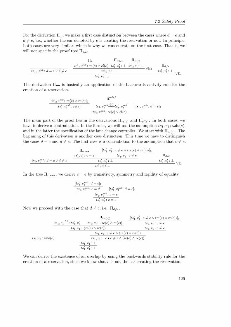
7.2 Safety Proof

For the derivation Π⊥, we make a first case distinction between the cases where d = e andd 6= e, i.e., whether the car denoted by e is creating the reservation or not. In principle,both cases are very similar, which is why we concentrate on the first case. That is, wewill not specify the proof tree Πd6=e.

ts1, vsub1 : d = e ∨ d 6= e

Π←−ts′1, v

sub1 : re(e) ∨ cl(e)

Πre(e)

ts′1, v′1 : ⊥

Πcl(e)

ts′1, v′1 : ⊥ ∨E3

ts′1, v′1 : ⊥

Πd 6=ets′1, v

′1 : ⊥ ∨E4

ts′1, v′1 : ⊥

The derivation Π←− is basically an application of the backwards activity rule for thecreation of a reservation.

[ts′1, vsub1 : re(e) ∧ re(c)]5

ts′1, vsub1 : re(e)

Πr(d),51

ts1, vsub1

r(d)−−→ts′1, vsub1 [ts1, vsub1 : d = e]4

ts′1, vsub1 : re(e) ∨ cl(e)

The main part of the proof lies in the derivations Πre(e) and Πcl(e). In both cases, wehave to derive a contradiction. In the former, we will use the assumption ts1, v1 : safe(e),and in the latter the specification of the lane change controller. We start with Πre(e). Thebeginning of this derivation is another case distinction. This time we have to distinguishthe cases d = c and d 6= c. The first case is a contradiction to the assumption that c 6= e.

ts1, vsub1 : d = c ∨ d 6= c

Πtrans

ts′1, v′1 : c = e

[ts′1, v′1 : c 6= e ∧ 〈re(e) ∧ re(c)〉]6

ts′1, v′1 : c 6= e

ts′1, v′1 : ⊥

Πd6=cts′1, v

′1 : ⊥ ∨E1

ts′1, v′1 : ⊥

In the tree Πtrans, we derive c = e by transitivity, symmetry and rigidity of equality.

[ts′1, vsub1 : d = c]1

ts′1, vsub1 : c = d [ts′1, v

sub1 : d = e]4

ts′1, vsub1 : c = e

ts′1, v′1 : c = e

Now we proceed with the case that d 6= c, i.e., Πd6=c.

ts1, v1 : safe(e)

ts1, v1r(d)−−→ts′1, v′1

Π〈re(e)〉ts1, v

′1 : 〈re(e) ∧ re(c)〉

ts1, v1 : 〈re(e) ∧ re(c)〉

[ts′1, v′1 : c 6= e ∧ 〈re(e) ∧ re(c)〉]6

ts′1, v′1 : c 6= e

ts1, v1 : c 6= e

ts1, v1 : c 6= e ∧ 〈re(e) ∧ re(c)〉ts1, v1 : ∃c • c 6= e ∧ 〈re(e) ∧ re(c)〉

ts1, v1 : ⊥ts′1, v

′1 : ⊥

We can derive the existence of an overlap by using the backwards stability rule for thecreation of a reservation, since we know that c is not the car creating the reservation.

129

7 Case study

[∆v′1]5

[ts1, vsub1 : re(e)]3


ts′1, vsub1 : re(c)

Πr(d),51

ts1, vsub1

r(d)−−→ts′1, vsub1 [ts1, vsub1 : d 6= c]1

ts1, vsub1 : re(c)

ts1, vsub1 : re(e) ∧ re(c)

ts1, v′1 : 〈re(e) ∧ re(c)〉

We are now finished with the case where a reservation of e was present on ts1, vsub1 and

turn our attention to the presence of a claim at this world, i.e., we create the derivationΠcl(e). In this part of the derivation, we will finally make use of our lane change controllerspecification. Like for the other case, we begin with a case distinction between d = c andd 6= c. The first case is derived similarly as before, and hence omitted. The idea for theother case is to derive an overlap between the claim of e and a reservation or claim of cand employ the controller specification to derive r(e)⊥. Then we can employ Substri toreplace e with d and get the desired contradiction.

ts1, vsub1 : d = c ∨ d 6= c

Πd=c

ts′1, v′1 : ⊥

ΠLC

ts1, v1 : r(e)⊥[ts′1, v

sub1 : d = e]4

ts1, v1 : d = e

ts1, v1 : r(d)⊥ ts1, v1r(d)−−→ts′1, v′1

ts′1, v′1 : ⊥ ∨E2

ts′1, v′1 : ⊥

In the derivation ΠLC, we use the controller specification and the fact the we could derivethat the potential collision check pc is satisfied.

Πpcc

ts1, v1 : ∃c • c 6= e ∧ 〈cl(e) ∧ (re(c) ∨ cl(c))〉

ts1, v1 : LC ts, v =⇒ ts1, v1ts1, v1 : ∀d • (∃c • pc(c, d)→ r(d)⊥)

ts1, v1 : ∃c • pc(c, e)→ r(e)⊥ts1, v1 : r(e)⊥

Now we can turn our attention to the derivation of the potential collision Πpcc. This issimilar to the case, where a reservation of e resides at the subview vsub1 , i.e., the final goalis to use the stability rule. But first, we have to introduce the existential quantifier, thesomewhere modality and replace v′1 by v1.

[ts′1, v′1 : c 6= e ∧ 〈re(e) ∧ re(c)〉]6

ts′1, v′1 : c 6= e

ts1, v1 : c 6= e

[∆v′1]5

[ts1, vsub1 : cl(e)]3

Πc

ts1, vsub1 : re(c)

ts1, vsub1 : re(c) ∨ cl(c)

ts1, vsub1 : cl(e) ∧ (re(c) ∨ cl(c))

ts1, v′1 : 〈cl(e) ∧ (re(c) ∨ cl(c))〉 ts1, v1

r(d)−−→ts′1, v′1ts1, v1 : 〈cl(e) ∧ (re(c) ∨ cl(c))〉

ts1, v1 : c 6= e ∧ 〈cl(e) ∧ (re(c) ∨ cl(c))〉ts1, v1 : ∃c • c 6= e ∧ 〈cl(e) ∧ (re(c) ∨ cl(c))〉

Finally, we arrive at the application of the stability rule in the derivation Πc.


ts′1, vsub1 : re(c)

Πr(d),51

ts1, vsub1

r(d)−−→ts′1, vsub1 [ts1, vsub1 : d 6= c]2

ts1, vsub1 : re(c)

130

7.2 Safety Proof

Now we constructed a well formed proof tree, where the only open assumptions are either

elements of Γ or of ts, v =⇒ ts1, v1, ts1, v1r(d)−−→ts′1, v′1, ts1, v1 : safe(e).

Lemma 7.2. The safety predicate is preserved if some car creates a claim, i.e.,

(Γ ∪ ts2, v2 : safe(e), ts, v =⇒ ts2, v2, ts2, v2c(d)−−→ts′2, v′2) ` ts′2, v′2 : safe(e) .

Proof. We begin like in the proof of Lemma 7.1 by presenting the root of the tree, tomotivate the upper parts of the derivation.

[ts′2, v′2 : ∃c • c 6= e ∧ 〈re(e) ∧ re(c)〉]5

[ts′2, v′2 : c 6= e ∧ 〈re(e) ∧ re(c)〉]4ts′2, v

′2 : 〈re(e) ∧ re(c)〉

Π⊥ts2, v2 : ⊥ts′2, v

′2 : ⊥ 〈〉E3

ts′2, v′2 : ⊥ ∃E4

ts′2, v′2 : ⊥ ¬I5

ts′2, v′2 : ¬∃c • c 6= e ∧ 〈re(e) ∧ re(c)〉

Now we have to show how to derive the contradiction on ts2, v2. This is done in the treeΠ⊥. Note the use of the view invariance over discrete transitions in the rule IV.

ts2, v2 : safe(e)

ts2, v2c(d)−−→ts′2, v′2

Π〈〉ts2, v

′2 : 〈re(e) ∧ re(c)〉

IVts2, v2 : 〈re(e) ∧ re(c)〉

[ts′2, v′2 : c 6= e ∧ 〈re(e) ∧ re(c)〉]4

ts′2, v′2 : c 6= e

ts2, v2 : c 6= e

ts2, v2 : c 6= e ∧ 〈re(e) ∧ re(c)〉ts2, v2 : ∃c • c 6= e ∧ 〈re(e) ∧ re(c)〉

ts2, v2 : ⊥

The tree Π〈〉 combines the results from the trees Πre(e)6=, Πre(e)= and Πre(c). We willonly show the trees concerning the variable e in detail, since Πre(c) is similar.

ts2, vsub2 : d 6= e ∨ d = e

Πre(e)6=


Πre(e)=

ts′2, vsub2 : re(e) ∨E1

ts2, vsub2 : re(e)

Πre(c)

ts2, vsub2 : re(c)

ts2, v′2 : re(e) ∧ re(c) [∆v′2

]3

ts2, v′2 : 〈re(e) ∧ re(c)〉

The trees Πre(e)6= and Πre(e)= are similar, with the exception that ts2, vsub2 : d 6= e has

to be substituted with ts2, vsub2 : d = e. The backwards stability rule for the creation of

claims is still applicable, since reservations are not changed while creating claims.



Πc(d),32

ts2, vsub2

c(d)−−→ts′2, vsub2 [ts2, vsub2 : d 6= e]1

ts2, vsub2 : re(e)

The derivation tree Πre(c) is similar to the tree consisting of Πre(e)=, Πre(e)6= and theapplication of a disjunction elimination ∨E2, where we substitute c for e.

131

7 Case study

Lemma 7.3. The safety predicate is preserved if some car withdraws one of its reserva-tions, i.e.,

(Γ ∪ ts3, v3 : safe(e), ts, v =⇒ ts3, v3, ts3, v3wd r(d)−−−−→ts′3, v′3) ` ts′3, v′3 : safe(e) .

Proof. The proof tree is structurally similar to the proof of Lemma 7.2, except that

all indices are changed to 3, all occurrences of ts2, v2c(d)−−→ts′2, v′2 are exchanged with

ts3, v3wd r(d)−−−−→ts′3, v′3 and all applications of

c(d)←−−S are substituted with applications ofwd r(d)←−−−−S.

Lemma 7.4. The safety predicate is preserved if some car withdraws its claim, i.e.,

(Γ ∪ ts4, v4 : safe(e), ts, v =⇒ ts4, v4, ts4, v4wd c(d)−−−−→ts′4, v′4) ` ts′4, v′4 : safe(e) .

Proof. Like the proof for Lemma 7.3, the proof tree is structurally similar to the proof ofLemma 7.2, with the appropriate changes.

Lemma 7.5. The safety predicate is preserved if time passes and accelerations change,i.e.,

(Γ ∪ ts5, v5 : safe(e), ts, v =⇒ ts5, v5, ts5, v5t−→ts′5, v′5) ` ts′5, v′5 : safe(e)

Proof. The root of the tree is similar to all the other derivations, i.e. we derive acontradiction on ts5, v5.

[ts′5, v′5 : ∃c • c 6= e ∧ 〈re(e) ∧ re(c)〉]3

Π〈〉ts5, v5 : 〈re(e) ∧ re(c)〉

[ts′5, v′5 : c 6= e ∧ 〈re(e) ∧ re(c)〉]2

ts′5, v′5 : c 6= e

ts5, v5 : c 6= e

ts5, v5 : c 6= e ∧ 〈re(e) ∧ re(c)〉ts5, v5 : ∃c • c 6= e ∧ 〈re(e) ∧ re(c)〉 ts5, v5 : safe(e)

ts5, v5 : ⊥ts′5, v

′5 : ⊥ ∃E2

ts′5, v′5 : ⊥ ¬I3

ts′5, v′5 : ¬∃c • c 6= e ∧ 〈re(e) ∧ re(c)〉

To derive the existence of an overlap on ts5, v5 in the tree Π〈〉, we use the definition of♦τ .

[ts′5, v′5 : c 6= e ∧ 〈re(e) ∧ re(c)〉]2ts′5, v

′5 : 〈re(e) ∧ re(c)〉 ts5, v5

t−→ts′5, v′5ts5, v5 : ♦τ 〈re(e) ∧ re(c)〉 ≡

ts5, v5 : ¬τ¬ 〈re(e) ∧ re(c)〉ΠDC

ts5, v5 : τ¬ 〈re(e) ∧ re(c)〉ts5, v5 : ⊥ ⊥E1

ts5, v5 : 〈re(e) ∧ re(c)〉In the following derivation ΠDC, we use the abbreviations

DC′ ≡ c 6= e→ (¬ 〈re(e) ∧ re(c)〉 → τ¬ 〈re(e) ∧ re(c)〉)and DC′d for DC′[e 7→ d].

132

7.3 Refining the Specification

ts, v : DC ts, v =⇒ ts5, v5

ts5, v5 : ∀c, d • DC′dts5, v5 : ∀d • DC′dts5, v5 : DC′

[ts′5, v′5 : c 6= e ∧ 〈re(e) ∧ re(c)〉]2

ts′5, v′5 : c 6= e

ts5, v5 : c 6= e

ts5, v5 : ¬ 〈re(e) ∧ re(c)〉 → τ¬ 〈re(e) ∧ re(c)〉 [ts5, v5 : ¬ 〈re(e) ∧ re(c)〉]1ts5, v5 : τ¬ 〈re(e) ∧ re(c)〉

Now we have constructed a well-formed derivation of the desired form.

We are now in the position to apply the invariance rule to get the desired result, i.e.,the safety predicate is an invariant under all transitions allowed by our controllers DCand LC.

Theorem 7.1. The safety predicate is an invariant for all cars using the controllerspecification given in Sect. 7.1, i.e.,

(ts, v : DC, ts, v : LC, ts, v : ∀e • safe(e), ∅) ` ts, v : ∀e •G safe(e) .

Proof. We can derive

(Γ, ∅) ` ts, v : safe(e)

with a single application of ∀E. Then we can employ Lemma 7.1 to Lemma 7.5, to getthe derivations needed for the application of G I, i.e.,

(Γ, ∅) ` ts, v : G safe(e) .

Observe that all application conditions of G I are satisfied, since each world tsi, vi onlyoccurs in the derivation of ts′i, v

′i : safe(e) and d (the car referred to in the dynamic

formulas) does not occur free in any element of Γ. As stated before, since e does notoccur free in any element of Γ, we can use ∀I to derive

(Γ, ∅) ` ts, v : ∀e •G safe(e) .


Now that we defined which rules a safe controller must adhere to, we give several examplesfor a more refined controller specification. However, the formulas LC and DC will still beat the heart of each of these specifications. Our modelling language is the combinationof traffic diagrams and EMLSL as presented in Chap. 6. Still, we will allow for manynon-deterministic choices of an actual controller implementation. In the following, weassume that the controller specification is a conjunction of both LC and DC as well asthe diagrams presented below.

First, we define several possible positive conditions for the creation of reservations.Note that the controller specification of Sect. 7.1 only restricts such transitions, but byno means ensures that any reservation will ever be created.

133

7 Case study

ego c[5,∞)

∃ c

r(ego)

(a) Reserving with Car Ahead

ego c

∃ c

r(ego)

(b) Reserving without Car Ahead

Figure 7.1: Positive Conditions for the Creation of Reservations

The diagram in Fig. 7.1a describes that the car ego may create a reservation, wheneverthe next car is at least 5 meters ahead. However, this condition will not ensure thecreation of any reservation, when no car c is present. Hence we also introduce the diagramin Fig. 7.1b, which explicitly states the absence of a car ahead of ego as a precondition.For reading these diagrams, recall that a diagram of the form

A B

is basically the implication A → B. Furthermore, by definition we know that Fφ ≡¬G¬φ, i.e., ¬Fφ ≡ G¬φ. So, using this equivalence and thinking of the faint temporalarrow as an invariance rather than an existence statement, the subdiagrams after thearrow can be thought of as an implication, where the left diagram implies the right one.Observe that we do not need to state that there exist no potential collisions for ego. Forif a potential collision existed as well as a situation satisfying e.g. Fig. 7.1a, the formulaLC implies that the creation of a reservation results in a contradiction, i.e., the transitionwould still not be allowed.

Figure 7.2 defines a liveness property for the withdrawal of reservations. The overallstructure is similar to the previous figures. However, the conclusion states only that therewill finally be a transition withdrawing one of the reservations. It does not ensure that aactual lane change happened and it does not require the withdrawal to happen within aspecified time frame.

For an upper bound for the withdrawal of a reservation, we would need a metricextension of the invariance modality. That is, the modality F [a,b]ϕ would ensure thatthere is an abstract transition, in which time between a and b passes and the resultingsnapshot satisfies ϕ. With the existing temporal modality i or the precise temporalarrows, we require that no discrete transitions apart from changes of accelerations occur.Hence we would needlessly (and unjustifiably) restrict the behaviour of all cars on thefreeway.

134


ego

ego

wd r(ego)

Figure 7.2: Withdrawal of Reservations

To specify that an actual lane change occurred, we would have to refer to the originallane of the car. In Fig. 7.2 however, we cannot distinguish anymore between the lane thecar started the lane change on and the target lane. We could try to overcome this problemby adding a layer denoting, e.g., that the upper lane contained the claim of ego in betweenthe unspecified space at the beginning of the sequence and the implication. However, thefaint temporal arrows are not expressive enough to state that the described withdrawal isthe first withdrawal of ego after the lane change. Still, the diagram describes a minimalliveness property every controller should satisfy.

We can also refine the behaviour of the distance controller for specific situations. Thetraffic diagrams in Fig. 7.3a and 7.3b describe behaviour of a distance controller whichadds more restrictions on DC. In particular, the diagrams ensure that whenever there isfree space in front of the car ego, this free space is preserved during time transitions. Thatis, similar to DC, the specifications of Fig. 7.3 do not restrict situations where overlapsoccur due to the creation of claims or reservations. The specification has to be split intotwo diagrams concerning situations outside and during a lane change manoeuvre, sincewe cannot distinguish the lanes during such a manoeuvre. If we just used Fig. 7.3a anddropped the condition that the car is not using two lanes at once, the specification wouldstill be satisfied if the free space on one lane was consumed, as long as the free space onthe other lane is preserved. Using both diagrams ensures the preservation of space inboth cases. Even though the diagrams seem to define a stronger controller at first sight,the property they ensure is weaker than DC. For example, if the reservation of a car cis directly adjacent to the reservation of ego, the diagrams do not guarantee anything,while DC still implies that the reservations will not overlap after an arbitrary time.

The diagrams given above only concretise the controller implemented in the car ego.For more concrete controller implementations for the rest of cars, we would have torepeat all these diagrams, replacing all occurrences of ego with a new variable d and

135

7 Case study

ego

ego

egoego

(a) Free Space Outside of a Lane Change

ego

ego

ego

ego

(b) Free Space During a Lane Change

Figure 7.3: Distance Controller Preserving Free Space in Front of Cars

quantifying d existentially for the sequences under the outermost negations. To avoidthis duplication, we could change the semantics of the quantifiers and remove the needfor the cars to be different from ego. Such a change would decrease the expressive powerof pure traffic diagrams, since ego could not be distinguished from other cars any more.However, in the combination with EMLSL, we could simply adjoin the inequality c 6= egofor each quantification of a variable c.

136

8Conclusion

Contents

8.1 Summary . . . . . . . . . . . . . . . . . . . . . . . . . . . . . . . 137

8.2 Future Work . . . . . . . . . . . . . . . . . . . . . . . . . . . . . 138

In this final chapter, we first summarise the content of the thesis in Sect. 8.1. Afterwards,in Sect. 8.2, we give several possibilities how the results of this work may be extended.

8.1 Summary

We presented an abstract model of freeway traffic, where space and its occupancy is themain focus. The dynamics of cars are mostly hidden within the model, and emphasis lieson the discrete changes cars may perform, in particular setting their turn signals andchanging lanes. Furthermore, we defined how the models are reduced to a finite part ofthe freeway, to give a notion of locality as basic parts the models.

Instances of these models serve as the semantic structures for the extended multi-lanespatial logic EMLSL. This logic takes methods from interval logics and typical modallogic, to form a many-dimensional multi-modal logic, which may be used to reason aboutfreeway traffic. Satisfiability of EMLSL formulas was shown to be undecidable, butnevertheless, we defined a proof system in the style of Natural Deduction, which wasproven to be sound. Several derived rules enhance the usability of the proof system.

To make the approach of this thesis more feasible to end-users, we presented the visuallanguage of Traffic Diagrams. To give an idea what types of properties are expressiblewith Traffic Diagrams, we gave exemplary diagrams which capture prominent featuresof the intended semantic model. The underlying structure of the depictions of TrafficDiagrams was formalised in terms of hypergraphs, which reflect both the diagrammaticelements, as well as important relations between these elements. We proved that each

137

8 Conclusion

diagram possesses a unique hypergraph as its type. Using these hypergraphs, we defineda semantics based on the same models as EMLSL. We sketched a possibility to decidesatisfiability of a subclass of Traffic Diagrams.

Since both EMLSL and Traffic Diagrams share the same semantic model, they may beused in combination to exploit the advantages of each language. We formalised such acombination by incorporating the formulas into the hypergraphs representing the syntaxof the diagrams. By showing the limits of Traffic Diagrams and defining a translationinto EMLSL, the diagrams were shown to be less expressive than the formulas.

Finally, we used EMLSL to present minimal specifications for two controller. The firstone avoids collisions while time passes, while the second one ensures a safe lane-change.This specification was proven to ensure safety for all possible transition sequences usingthe proof system for EMLSL. We then use different Traffic Diagrams to refine thisspecification, e.g., to guarantee a limited form of liveness.

8.2 Future Work

In this section, we describe possibilities to extend the work presented in the thesis. Eventhough most of these extensions affect the model itself, e.g., to incorporate notionsof robustness or different topologies, other extensions concern tool support and theidentification of new decidable subsets of the formalisms.

Different Models of Sensors As stated in Chap. 3, we only considered settings whereevery car knows both the position and safety envelope of all other cars within its view.Obviously, such a requirement needs perfect sensors installed in the cars. If we permitmore realistic implementations of sensors, i.e., a situation where each car knows its owndistance needed for an emergency braking and only the physical size of the other cars,our approach does not ensure safety of traffic anymore. Within such a setting explicitcommunication is needed for a safe lane-change protocol, as shown in previous work[Hil+11]. Hence to reason about safety in such a setting, we need to incorporate meansof describing communications between several agents within our logic. Furthermore, weprobably need methods to relate views of different owners to each other. That is, thecurrent emphasis on a single, distinguished car has to be more explicit within the logicitself, with additional syntactic elements to switch views within a single formula.

Robustness Another possibility to increase the realism of our model is to allow forincorrect sensor values, within certain bounds. That is, instead of the exact satisfactionrelation defined in Chap. 4, a more robust notion allowing for small deviances is needed.This also leads to the question, into which parts of the model such disturbances shouldbe introduced. It seems reasonable to at least allow for errors in distances measurements,since these are dependent on sensor readings. Similarly, no car can possibly ensure tochange its state at a single point in time, which implies that robustness within transitionsmay also be considered. In particular, that the discrete transitions of Chap. 3 do nottake any time has to be questioned.

138

8.2 Future Work

Synchronous Parallelism Even though traffic on freeways can be thought of as aninherently parallel system of multiple agents, our model is defined using an interleavingsemantics. That is, no two transitions occur exactly simultaneously. In particular, inevery trace, the order of consecutive discrete transitions is fixed, while the transitionsmay stem from different cars. However, in a system of multiple, autonomous agents, amodel of true concurrency is more realistic. Hence the labelled transition system impliedby our model could be replaced by either an event structure or a distributed transitionsystem [Lod+92], which both allow for the simultaneous occurrence of transitions.

Connecting the Abstract Model with Dynamics We presented only a simple definitionof the dynamics in Chap. 3. For concrete implementations, our approach has to beconnected with more concrete specifications, e.g., in terms of hybrid automata or simplydifferential equations. A concrete model of the dynamical behaviour of cars has to fulfilseveral constraints. It has to able to return the length needed for a safe emergencybraking to the upper level (i.e., it has to compute the values of the sensor function atleast for the current, distinguished car), and it has to ensure that each car only drives onthe lanes it reserved. Furthermore, the dynamical model has to ensure, that the cars aswell as the values of the sensor function only evolve continuously.

Increasing the Domain of Application To analyse different scenarios, the abstractmodel has to be changed severely. Even though, oncoming traffic may be incorporatedrather easily [HLO13], modelling urban traffic scenarios, i.e., crossings, is more of achallenge. The topology of the model has to be changed drastically to allow for differentstreets to cross. However, vastly different topologies may also be of interest to describeother traffic scenarios, for example airborne traffic, where air planes reserve corridors inthree-dimensional space. Furthermore, lanes which follow certain trajectories may beuseful to reason about shipping traffic.

Decidability As shown in Chap. 4, our main tool of reasoning, the logic EMLSL, isundecidable in general. It is not directly obvious, what restrictions on the model or thesyntax yield decidable subsets. A promising approach is to restrict the number of cars tobe finite, to get a translation into a decidable subset of Schafer’s Shape Calculus [Sch07].Restricting the number and nesting of chops is also sensible to use the “dove-tailing”approach of Gabbay [Gab98; Gab+03]. The satisfiability problem of atomic spatialdiagrams probably is decidable, as sketched in Chap. 5. However, the procedure stillhas to be formally proven correct, and enhanced to cope with a larger subset of TrafficDiagrams.

Tool Support Several parts of the work in this thesis suggest the implementation of atool, or rather a framework incorporating different tools. The proof system presented inChap. 4 could be implemented within a general theorem prover. Isabelle [Pau94] seemslike a suitable selection, since it is based on natural deduction, and since several labelleddeductive systems for modal- and interval logics have already been implemented within

139

8 Conclusion

Isabelle [BMV98; Ras02; Vig00]. For the diagrammatic system of Chap. 5, a graphicaleditor is of inherent importance, to ease the use and creation of diagrams. With such aneditor, an implementation of the translation given in Chap. 6 is sensible to gain a directconnection between the implementations of both. Then, techniques for heterogeneousreasoning as implemented in, e.g., the Diabelli system [UJ12] can probably be adaptedto our setting.

140

Bibliography

[AB96] G. Allwein and J. Barwise, eds. Logical Reasoning with Diagrams. OxfordUniversity Press, 1996.

[Abr10] J.-R. Abrial. Modeling in Event-B: System and Software Engineering. Cam-bridge University Press, 2010.

[AER98] M. Andries, G. Engels, and J. Rekers. “How to Represent a Visual Speci-fication”. In: Visual Language Theory. Ed. by K. Marriott and B. Meyer.Springer, 1998.

[All83] J. F. Allen. “Maintaining knowledge about temporal intervals”. In: Commu-nications of the ACM 26.11 (1983), pp. 832–843.

[APB07] M. Aiello, I. Pratt-Hartmann, and J. van Benthem, eds. Handbook of SpatialLogics. Springer, 2007.

[Bar+08] D. Barker-Plummer, J. Etchemendy, A. Liu, M. Murray, and N. Swoboda.“Openproof-a flexible framework for heterogeneous reasoning”. In: Diagram-matic Representation and Inference – International Conference on the Theoryand Applications of Diagrams – DIAGRAMS 2008. Ed. by G. Stapleton,J. Howse, and J. Lee. Vol. 5223. LNAI. Springer, 2008, pp. 347–349.

[BB13] R. Banach and M. Butler. “Cruise Control in Hybrid Event-B”. In: Inter-national Colloquium on Theoretical Aspects of Computing – ICTAC 2013.Ed. by Z. Liu, J. Woodcock, and Huibiao Z. Vol. 8049. LNCS. Springer, 2013,pp. 76–93.

[BB14] R. Banach and M. Butler. “A Hybrid Event-B Study of Lane Centering”.In: International Conference on Complex Systems Design & Management –CSD&M 2013. Ed. by M. Aiguier, F. Boulanger, D. Krob, and C. Marchal.Springer, 2014, pp. 97–111.

[BE90] J. Barwise and J. Etchemendy. “Information, Infons, and Inference”. In:Situation Theory and its applications. Ed. by R. Cooper, K. Mukai, andJ. Perry. Vol. 1. CSLI Lecture Notes Number 22. CSLI: Center for the Studyof Language and Information, 1990, pp. 33–78.

[BE92] J. Barwise and J. Etchemendy. “Hyperproof: Logical reasoning with dia-grams”. In: Working Notes of the AAAI Spring Symposium on Reasoningwith Diagrammatic Representations. 1992.

141

Bibliography

[BE96] J. Barwise and J. Etchemendy. “Heterogeneous Logic”. In: Logical Reasoningwith Diagrams. Ed. by G. Allwein and J. Barwise. Oxford University Press,1996, pp. 179–200.

[Bea06] J. M. L. Bean. “Ribbon Proofs: A Proof System for the Logic of BunchedImplications”. PhD thesis. 2006.

[Ben86] E. Bencivenga. “Free Logics”. In: Handbook of Philosophical Logic. Ed. byD. M. Gabbay and F. Guenthner. Vol. 166. Springer, 1986, pp. 373–426.

[BKK03] P. Baldan, B. Konig, and B. Konig. “A Logic for Analyzing Abstractionsof Graph Transformation Systems”. In: International Symposium on StaticAnalysis – SAS 2003. Ed. by R. Cousot. Vol. 2694. LNCS. Springer, 2003,pp. 255–272.

[BMV98] D. Basin, S. Matthews, and L. Vigano. “Natural Deduction for Non-ClassicalLogics”. In: Studia Logica 60 (1 1998), pp. 119–160.

[BRZ99] R. Barua, S. Roy, and Zhou C. “Completeness of Neighbourhood Logic”. In:Symposium on Theoretical Aspects of Computer Science – STACS 99. Ed. byC. Meinel and S. Tison. Vol. 1563. LNCS. Springer, 1999, pp. 521–530.

[Bya+09] A. B. Byachkov, C. Cattani, E. M. Nosova, and M. P. Yushkov. “The SimplestModel of the Turning Movement of a Car with its Possible Sideslip”. In:TECHNISCHE MECHANIK 29.1 (2009), pp. 1–12.

[CC01] L. Caires and L. Cardelli. “A spatial logic for concurrency (Part I)”. In:International Symposium on Theoretical Aspects of Computer Software –TACS 2001. Ed. by N. Kobayashi and B. C. Pierce. Vol. 2215. LNCS. Springer.2001, pp. 1–37.

[CC04] L. Caires and L. Cardelli. “A spatial logic for concurrency (Part II)”. In:Theoretical Computer Science 322.3 (2004), pp. 517–565.

[CG98] L. Cardelli and A. D Gordon. “Mobile ambients”. In: International Conferenceon Foundations of Software Science and Computation Structures – FoSSaCS1998. Ed. by M. Nivat. Vol. 1378. LNCS. Springer. 1998, pp. 140–155.

[Coo72] D. C. Cooper. “Theorem proving in arithmetic without multiplication”. In:Machine Intelligence 7.91–99 (1972), p. 300.

[CSS05] C. Caleiro, A. Sernadas, and C. Sernadas. “Fibring Logics: Past, Present andFuture”. In: We Will Show Them! Essays in Honour of Dov Gabbay, Volume1. Ed. by S. Artemov, H. Barringer, A. d’Avila Garcez, L. C. Lamb, andJ. Woods. Colledge Publications, 2005, pp. 363–388.

[CSS11] M. E. Coniglio, A. Sernadas, and C. Sernadas. “Preservation by fibring of thefinite model property”. In: Journal of Logic and Computation 21.2 (2011),pp. 375–402.

[Dau04a] F. Dau. The Logic System of Concept Graphs with Negation. Vol. 2892. LNAI.Springer, 2004.

142

Bibliography

[Dau04b] F. Dau. “Types and Tokens for Logic with Diagrams”. In: InternationalConference on Computational Science – ICCS 2004. Ed. by M. Bubak, G. D.van Albada, P. M. A. Sloot, and J. Dongarra. Vol. 3038. LNCS. Springer,2004, pp. 62–93.

[Dau09] F. Dau. “The Advent of Formal Diagrammatic Reasoning Systems”. In:International Conference on Formal Concept Analysis – ICFCA 2009. Ed. byS. Ferre and S. Rudolph. Vol. 5548. LNCS. Springer, 2009, pp. 38–56.

[DH01] W. Damm and D. Harel. “LSCs: Breathing Life into Message SequenceCharts”. In: Formal Methods in System Design 19 (Jan. 2001), pp. 45–80.

[DHO06] W. Damm, H. Hungar, and E.-R. Olderog.“Verification of Cooperating TrafficAgents”. In: International Journal of Control 79.5 (2006), pp. 395–421.

[DMR14] W. Damm, E. Mohlmann, and A. Rakow. “Component Based Design ofHybrid Systems: A Case Study on Concurrency and Coupling”. In: Inter-national Conference on Hybrid Systems: Computation and Control – HSCC2014. Ed. by M. Franzle and J. Lygeros. ACM, 2014, pp. 145–150.

[Dut95] B. Dutertre. “Complete Proof Systems for First Order Interval TemporalLogic”. In: IEEE Symposium on Logic in Computer Science – LICS 1995.Ed. by D. C. Kozen. IEEE Computer Society, 1995, pp. 36–43.

[EC82] E. A. Emerson and E. M. Clarke. “Using branching time temporal logic tosynthesize synchronization skeletons”. In: Science of Computer Programming2.3 (1982), pp. 241–266.

[ES99] M. Erwig and M. Schneider. “Visual Specification of Spatio-Temporal De-velopments”. In: IEEE International Symposium on Visual Languages – VL1999. IEEE Computer Society, 1999, pp. 187–188.

[Fab+11] J. Faber, S. Linker, E.-R. Olderog, and J.-D. Quesel. “Syspect - Modelling,Specifying, and Verifying Real-Time Systems with Rich Data”. In: Interna-tional Journal of Software and Informatics 5.1-2 (2011), pp. 117–137.

[FG92] M. Finger and D. M Gabbay. “Adding a temporal dimension to a logicsystem”. In: Journal of Logic, Language and Information 1.3 (1992), pp. 203–233.

[FM98] M. Fitting and R. L. Mendelsohn. First-Order Modal Logic. Springer, 1998.

[FR75] J. Ferrante and C. Rackoff. “A decision procedure for the first order theoryof real addition with order”. In: SIAM Journal on Computing 4.1 (1975),pp. 69–76.

[Gab+03] D. M. Gabbay, A. Kurucz, F. Wolter, and M. Zakharyaschev. Many-dimensional modal logics: Theory and applications. Vol. 148. Studies in logicand the foundations of mathematics. Elsevier, 2003.

[Gab96] D. M. Gabbay. Labelled deductive systems. Vol. 1. Oxford Logic Guides.Oxford University Press, 1996.

143

Bibliography

[Gab98] D. M. Gabbay. Fibring logics. Oxford Logic Guides. Oxford University Press,1998.

[Gen35] G. Gentzen. “Untersuchungen uber das logische Schließen. I”. In: Mathema-tische Zeitschrift 39 (1 1935), pp. 176–210.

[Haa98] V. Haarslev. “A Fully Formalized Theory for Describing Visual Notations”.In: Visual Language Theory. Ed. by K. Marriott and B. Meyer. Springer,1998.

[Ham96] E. Hammer. “Peircean Graphs for Propositional Logic”. In: Logical Reasoningwith Diagrams. Ed. by G. Allwein and J. Barwise. Oxford University Press,1996, pp. 129–147.

[Har88] D. Harel. “On Visual Formalisms”. In: Communications of the ACM 31.5(1988).

[Hil+11] M. Hilscher, S. Linker, E.-R. Olderog, and A. P. Ravn. “An Abstract Modelfor Proving Safety of Multi-lane Traffic Manoeuvres”. In: Formal Methodsand Software Engineering – International Conference on Formal EngineeringMethods – ICFEM 2011. Ed. by Z. Qiu S. Qin. LNCS. Springer, 2011, pp. 404–419.

[Hil14] M. Hilscher. Private communications. 2014.

[HLO13] M. Hilscher, S. Linker, and E.-R. Olderog. “Proving Safety of Traffic Manoeu-vres on Country Roads”. In: Theories of Programming and Formal Methods– Essays Dedicated to Jifeng He on the Occasion of His 70th Birthday. Ed.by Z. Liu, J. Woodcock, and Huibiao Z. Vol. 8051. LNCS. Springer, 2013,pp. 196–212.

[Hoa69] C. A. R. Hoare. “An Axiomatic Basis for Computer Programming”. In:Communications of the ACM 12.10 (1969), pp. 576–580.

[Hoe06] J. Hoenicke. “Combination of Processes, Data, and Time”. PhD thesis. Carlvon Ossietzky Universitat Oldenburg, 2006.

[How+02] J. Howse, F. Molina, S.-J. Shin, and J. Taylor. “On Diagram Tokens andTypes”. In: Diagrammatic Representation and Inference – InternationalConference on the Theory and Applications of Diagrams – DIAGRAMS2002. Ed. by M. Hegarty, B. Meyer, and N. H. Narayanan. Vol. 2317. LNAI.Springer, 2002, pp. 146–160.

[HP08] I. A. Hansen and J. Pachl, eds. Railway Timetable & Traffic – Analysis,Modelling, Simulation. Eurailpress, 2008.

[HP09] A. Habel and K.-H. Pennemann.“Correctness of high-level transformation sys-tems relative to nested conditions”. In: Mathematical Structures in ComputerScience 19 (02 Apr. 2009), pp. 245–296.

[HR10] A. Habel and H. Radke. “Expressiveness of graph conditions with variables”.In: Electronic Communications of the EASST 30 (2010).

144

Bibliography

[HS91] J. Y. Halpern and Y. Shoham. “A Propositional Modal Logic of Time Inter-vals”. In: Journal of the ACM 38.4 (Oct. 1991), pp. 935–962.

[Hsu+94] A. Hsu, F. Eskafi, S. Sachs, and P. Varaija. “Protocol design for an automatedhighway system”. In: Discrete Event Dynamic Systems 2.1 (1994), pp. 183–206.

[ITU96] International Telecommunication Union (ITU). Z.120. ITU-TS recommenda-tion Z.120: Message Sequence Chart (MSC). 1996.

[JKI99] H. Jula, E. B. Kosmatopoulos, and P. A. Ioannou. Collision AvoidanceAnalysis for Lane Changing and Merging. Tech. rep. UCB-ITS-PRR-99-13.California Partners for Advanced Transit and Highways (PATH), Universityof California at Berkeley, 1999.

[KE14] S. Kemper and C. Etzien. “A Visual Logic for the Description of HighwayTraffic Scenarios”. In: International Conference on Complex Systems Design& Management – CSD&M 2013. Ed. by M. Aiguier, F. Boulanger, D. Krob,and C. Marchal. Springer, 2014, pp. 233–245.

[Ken97] S. Kent. “Constraint diagrams: visualizing invariants in object-oriented mod-els”. In: ACM SIGPLAN Conference on Object-Oriented Programming, Sys-tems, Languages & Applications – OOPSLA 1997. Ed. by M. E. S. Loomis,T. Bloom, and A. M. Berman. ACM, 1997, pp. 327–341.

[Kle00] C. Kleuker. “Constraint Diagrams”. PhD thesis. Carl von Ossietzky Univer-sitat Oldenburg, 2000.

[Koo+08] P. Koonce, L. Rodegerdts, K. Lee, S. Quayle, S. Beaird, C. Braud, J. Bonneson,P. Tarnoff, and T. Urbanik. Traffic Signal Timing Manual. Tech. rep. U.S.Department of Transportation, Federal Highway Administration, 2008.

[LGS98] J. Lygeros, D. N. Godbole, and S. Sastry. “Verified hybrid controllers forautomated vehicles”. In: IEEE Transactions on Automatic Control 43.4(1998), pp. 522–539.

[LH13] S. Linker and M. Hilscher. “Proof theory of a multi-lane spatial logic”. In:International Colloquium on Theoretical Aspects of Computing – ICTAC2013. Ed. by Z. Liu, J. Woodcock, and Huibiao Z. Vol. 8049. LNCS. Springer,2013, pp. 231–248.

[Lin07] S. Linker. “Naturliches Schließen fur den Shape Calculus”. http://www.uni-oldenburg.de/fileadmin/user_upload/f2inform-csd/linker07.pdf.Minor thesis. Carl von Ossietzky Universitat Oldenburg, 2007.

[Lin10] S. Linker. “Diagrammatic Specification of Mobile Real-Time Systems”. In:Diagrammatic Representation and Inference – International Conference onthe Theory and Applications of Diagrams – DIAGRAMS 2010. Ed. by A. K.Goel, M. Jamnik, and N. H. Narayanan. Vol. 6170. LNAI. Springer, 2010,pp. 316–318.

145

http://www.uni-oldenburg.de/fileadmin/user_upload/f2inform-csd/linker07.pdf

http://www.uni-oldenburg.de/fileadmin/user_upload/f2inform-csd/linker07.pdf

Bibliography

[Lod+92] K. Lodaya, M. Mukund, R. Ramanujam, and P.S. Thiagarajan. “Modelsand logics for true concurrency”. In: Sadhana (Academy Proceedings inEngineering Sciences). Vol. 17. 1. Indian Academy of Sciences. 1992, pp. 131–165.

[LPN11] S. M. Loos, A. Platzer, and L. Nistor. “Adaptive Cruise Control: Hybrid,Distributed, and Now Formally Verified”. In: International Symposium onFormal Methods – FM 2011. Ed. by M. Butler and W. Schulte. Vol. 6664.LNCS. Springer, 2011, pp. 42–56.

[MA08] J. McDermott and G. Allwein. “A Formalism for Visual Security Proto-col Modeling”. In: Journal of Visual Languages & Computing 19.2 (2008),pp. 153–181.

[McD05] J. P. McDermott. A Formal Syntax and Semantics for the GSPML Language.Tech. rep. Naval Research Laboratory, Information Technology Division,2005.

[Min00] M. Minas. “Hypergraphs as a Uniform Diagram Representation Model”. In:Selected Papers of the International Workshop on Theory and Applicationof Graph Transformations – TAGT 1998. Ed. by H. Ehrig, G. Engels, H.-J.Kreowski, and G. Rozenberg. Vol. 1764. LNCS. Springer, 2000, pp. 281–295.

[Min67] M. L. Minsky. Computation: finite and infinite machines. Prentice-Hall, 1967.

[Mos85] B. C. Moszkowski. “A Temporal Logic for Multilevel Reasoning about Hard-ware”. In: Computer 18.2 (1985), pp. 10–19.

[MOT10] K. Mineshima, M. Okada, and R. Takemura. “Two Types of DiagrammaticInference Systems: Natural Deduction Style and Resolution Style”. In: Di-agrammatic Representation and Inference – International Conference onthe Theory and Applications of Diagrams – DIAGRAMS 2010. Ed. by A..Goel, M. Jamnik, and N. H. Narayanan. Vol. 6170. LNCS. Springer, 2010,pp. 99–114.

[MP95] Z. Manna and A. Pnueli. Temporal Verification of Reactive Systems: Safety.Springer, 1995.

[MPW92] R. Milner, J. Parrow, and D. Walker. “A Calculus of Mobile Processes, I”. In:Information and Computation 100.1 (Sept. 1992), pp. 1–40.

[MV95] M. Minas and G. Viehstaedt. “DiaGen: a generator for diagram editorsproviding direct manipulation and execution of diagrams”. In: IEEE Inter-national Symposium on Visual Languages – VL 1995. Ed. by V. Haarslev.IEEE Computer Society, 1995, pp. 203–210.

[MV97] M. Marx and Y. Venema. Multi-dimensional modal logic. Springer, 1997.

[Pau94] L. Paulson. Isabelle: A Generic Theorem Prover. Springer, 1994.

[Pla10a] A. Platzer. Logical Analysis of Hybrid Systems: Proving Theorems for Com-plex Dynamics. Springer, 2010.

146

Bibliography

[Pla10b] A. Platzer. “Quantified Differential Dynamic Logic for Distributed HybridSystems”. In: EACSL Conference on Computer Science Logic – CSL 2010.Ed. by A. Dawar and H. Veith. Vol. 6247. LNCS. Springer, 2010, pp. 469–483.

[Pnu77] A. Pnueli. “The Temporal Logic of Programs”. In: IEEE Symposium onFoundations of Computer Science – SFCS 1977. IEEE Computer Society,1977, pp. 46–57.

[PQ09] A. Platzer and J.-D. Quesel. “European Train Control System: A Case Studyin Formal Verification”. In: Formal Methods and Software Engineering –International Conference on Formal Engineering Methods – ICFEM 2009.Ed. by A. Cavalcanti and K. Breitman. Vol. 5885. LNCS. Springer, 2009,pp. 246–265.

[Pra06] D. Prawitz. Natural Deduction: A Proof-theoretical Study. Dover, 2006.

[Pri57] A. N. Prior. Time and Modality. Oxford University Press, 1957.

[Rad13] H. Radke. “HR* Graph Conditions Between Counting Monadic Second-Orderand Second-Order Graph Formulas”. In: Electronic Communications of theEASST 61 (2013).

[Ras+02] J. Rasga, A. Sernadas, C. Sernadas, and L. Vigano. “Fibring Labelled Deduc-tion Systems”. In: Journal of Logic and Computation 12.3 (2002), pp. 443–473.

[Ras01] T. M. Rasmussen. “Labelled Natural Deduction for Interval Logics”. In:EACSL Conference on Computer Science Logic – CSL 2001. Ed. by L.Fribourg. Vol. 2142. LNCS. Springer, 2001, pp. 308–323.

[Ras02] T. M. Rasmussen. “Interval logic. Proof theory and theorem proving”. PhDthesis. Technical University of Denmark, 2002.

[RCC92] D. A. Randell, Z. Cui, and A. G. Cohn. “A Spatial Logic based on Regionsand Connection”. In: International Conference on Principles of KnowledgeRepresentation and Reasoning – KR 1992. Ed. by B. Nebel, C. Rich, andW. Swartout. Morgan Kaufmann, 1992, pp. 165–176.

[Rey02] J. C. Reynolds. “Separation Logic: A Logic for Shared Mutable Data Struc-tures”. In: IEEE Symposium on Logic in Computer Science – LICS 2002.Ed. by G. D. Plotkin. IEEE Computer Society, 2002, pp. 55–74.

[RJB04] J. Rumbaugh, I. Jacobson, and G. Booch. The Unified Modeling LanguageReference Manual (2nd Edition). Pearson Higher Education, 2004.

[Roz97] G. Rozenberg, ed. Handbook of graph grammars and computing by graphtransformation: volume I. foundations. World Scientific Publishing, 1997.

[RS95] J. Rekers and A. Schurr. “A graph grammar approach to graphical parsing”.In: IEEE International Symposium on Visual Languages – VL 1995. Ed. byV. Haarslev. IEEE Computer Society, 1995, pp. 195–202.

[Sch01] R. C. Schlor. “Symbolic Timing Diagrams: A Visual Formalism for ModelVerification”. PhD thesis. Carl von Ossietzky Universitat Oldenburg, 2001.

147

Bibliography

[Sch05] A. Schafer. “A calculus for shapes in time and space”. In: InternationalColloquium on Theoretical Aspects of Computing – ICTAC 2004. Ed. by Z.Liu and K. Araki. Vol. 3407. LNCS. Springer, 2005, pp. 463–478.

[Sch07] A. Schafer. “Axiomatisation and decidability of multi-dimensional DurationCalculus”. In: Information and Computation 205.1 (2007). Special Issue:TIME 2005, pp. 25–64.

[Sch14] M. Schwammberger.“Semantik von Controllern fur sicheren Fahrspurwechsel”.Master’s Thesis. Carl von Ossietzky Universitat Oldenburg, 2014.

[Sha+13] Z. Shao, J. Liu, Z. Ding, M. Chen, and N. Jiang. “Spatio-Temporal PropertiesAnalysis for Cyber-Physical Systems”. In: Engineering of Complex ComputerSystems – ICECCS 2013. IEEE. 2013, pp. 101–110.

[Shi04] S.-J. Shin. “Heterogeneous Reasoning and its Logic”. In: Bulletin of SymbolicLogic 10.1 (2004), pp. 86–106.

[Shi95] S.-J. Shin. The logical status of diagrams. Cambridge: Cambridge UniversityPress, 1995.

[Sim94] A. K. Simpson. “The Proof Theory and Semantics of Intuitionistic ModalLogic”. PhD thesis. University of Edinburgh, 1994.

[SM07] G. Stapleton and J. Masthoff. “Incorporating Negation into Visual Logics: ACase Study Using Euler Diagrams”. In: Visual Languages and Computing(2007), pp. 187–194.

[Smi00] G. Smith. The Object-Z Specification Language. Springer, 2000.

[Sta+05] G. Stapleton, S. Thompson, A. Fish, J. Howse, and J. Taylor. “A NewLanguage for the Visualization of Logic and reasoning”. In: InternationalConference on Distributed Multimedia Systems – DMS 2005. Ed. by P. Coxand T. Smedley. Knowledge Systems Institute, 2005, pp. 287–292.

[Tob08] T. Toben. “Counterexample Guided Spotlight Abstraction Refinement”. In:International Conference on Formal Techniques for Networked and DistributedSystems -– FORTE 2008. Ed. by K. Suzuki, T. Higashino, K. Yasumoto, andK. El-Fakih. Vol. 5048. LNCS. Springer, 2008, pp. 21–36.

[UJ12] M. Urbas and M. Jamnik. “Diabelli: A heterogeneous proof system”. In:International Joint Conference on Automated Reasoning – IJCAR 2012.Ed. by B. Gramlich, D. Miller, and U. Sattler. Vol. 7364. LNAI. Springer,2012, pp. 559–566.

[UJ14] M. Urbas and M. Jamnik. “A Framework for Heterogeneous Reasoningin Formal and Informal Domains”. In: Diagrammatic Representation andInference – International Conference on the Theory and Applications ofDiagrams – DIAGRAMS 2014. Ed. by T. Dwyer, H. Purchase, and A. Delaney.Vol. 8578. LNAI. Springer, 2014, pp. 277–292.

[UML12] Unified Modeling Language (UML): Superstructure version 2.4.1. formal/2012-05-07. 2012. url: http://www.omg.org.

148

http://www.omg.org

Bibliography

[Urb+12] M. Urbas, M. Jamnik, G. Stapleton, and J. Flower.“Speedith: a diagrammaticreasoner for spider diagrams”. In: Diagrammatic Representation and Inference– International Conference on the Theory and Applications of Diagrams –DIAGRAMS 2012. Ed. by P. T. Cox, B. Plimmer, and P. Rodgers. Vol. 7352.LNAI. Springer, 2012, pp. 163–177.

[Vig00] L. Vigano. Labelled Non-Classical Logics. Kluwer Academic Publishers, 2000.

[WDP13] J. Wickerson, M. Dodds, and M. Parkinson. “Ribbon proofs for separationlogic”. In: Programming Languages and Systems – European Symposium onProgramming – ESOP 2013. Ed. by M. Felleisen and P. Gardner. Vol. 7792.LNCS. Springer, 2013, pp. 189–208.

[WW07] B. Wachter and B. Westphal. “The spotlight principle”. In: InternationalConference on Verification, Model Checking, and Abstract Interpretation –VMCAI 2007. Ed. by B. Cook and A. Podelski. Vol. 4349. LNCS. Springer.2007, pp. 182–198.

[ZHR91] Zhou C., C. A. R. Hoare, and A. P. Ravn. “A Calculus of Durations”. In:Information Processing Letters 40.5 (1991), pp. 269–276.

[ZHS93] Zhou C., M. R. Hansen, and P. Sestoft. “Decidability and undecidabilityresults for duration calculus”. In: Symposium on Theoretical Aspects ofComputer Science – STACS 1993. Ed. by P. Enjalbert, A. Finkel, and K.W.Wagner. Vol. 665. LNCS. Springer, 1993, pp. 58–68.

149

Index

Symbol Index

:, 27, 37, 27, 37

acc, 21

∗, 32`, 34τ , 34

clmV , 28CVar, 31a , 7, 32clm, 21cl , 32|=M , 99|= (HR∗ condition), 15|= (diagrams), 98|= (formulas), 33|= (labelled formulas), 38|= (relational formulas), 38|=S , 99cC , 105ciR, 105cl, 105cr, 105

∆, 38∆v′i

, 128Z⇒p, 12Z⇒∗, 13D, 75♦`, 34DC, 126dri, 39

E , 11ego, 32[·], 33∃(P w C, c), 14∃(h, c), 14E, 37

FX , 104

FL, 104F , 34Φ, 32ts, v : φ, 37w : ϕ, 9φr, 35

Γ, 38G , 32G, 11

halt, 62hcf, 39hri, 39

I, 20init, 60I, 6I, 6IVar, 6

lenV , 28L, 20L, 25l, 11LC, 127LVar, 32`, 32λ, 38

marker, 60·M, 113mv , 26mutex, 60

N, 5

, 6O, 11, 101

Per , 60Π∗,ji , 128

150

SYMBOL INDEX

P, 5pc, 126periodic, 61pos, 21`, 39

·Q, 114

R+ , 6resV , 28R∗, 6R, 6res, 21ρ, 37re, 32RVar, 32, 71ri, 39

[· 7→ ·], 9safe, 126〈·〉 (sequence), 6σ, 38〈·〉 (modality), 33spd , 21

t , 23acc(C,a)−−−−−→ , 23t−→ , 23c(C,n)−−−−→ , 22r(C)−−→ , 22wd c(C)−−−−−→ , 22wd r(C,n)−−−−−−→ , 23T S, 21TS, 21T, 20=⇒, 24, 37Θ, 32ts, 37TS, 37τ , 11θ, 32E, 37·T , 115

c(c)−−→, 37r(c)−−→, 37wd c(c)−−−−→, 37wd r(c)−−−−→, 37t−→, 37θ, 11T , 11TT , 81TNT , 81

V , 25V L, 25VX , 25v, 37v, 105v, 105ν, 32νI , 97νV , 32Var, 32, 70vcf, 39V, 11V, 37vri, 39vl, 105vr, 105

ω, 32

X, 25χ, 98⊕· 7→ ·, 6

ΩE , 27

151

Index

Subject Index

advanced driver assistance system, 108application (graph rewriting), 12arithmetic

Presburger, 106real, 106

assumption elimination, 8atom

equality, 32free, 35spatial, 32

attachment function, 11axiom (graph rewriting), 13

caraction, 71braking distance, 19physical size, 19safety envelope, 19, 27

chop-free, 11claim, 21, 72

creation, 23withdrawal, 23

composition, 6

derivation, 8, 39derivation (graph rewriting), 13diagram

spatial, 74Traffic Diagram, 75

distance arrow, 73distance controller, 126domain, 6

edge, 11EMLSL, 31expressivity, 111

flexible, 8, 35formula, 32

dynamic, 37labelled, 9, 37locality, 37

relational, 9, 37timing, 37

function, 6modification, 6

global contradiction, 9graph homomorphism, 11graph rewriting, 13

Traffic Diagrams, 83graph rewriting rule, 12graph substitution, 14

HR∗ condition, 13heterogeneous reasoning, 121horizon, 25hyperedge replacement, 13hypergraph, 11

image, 6implicit lengths, 98interlingua, 123interval, 6, 71

chop, 27variable, 6, 71

labelled natural deduction, 9EMLSL, 36

labelling algebra, 36lane change controller, 127lane separation, 73lane sequence, 73layer, 74

full, 74partial, 74

left-hand side, 12logic

computational tree logic (CTL), 7interval temporal logic (ITL), 7linear temporal logic (LTL), 7signed interval logic (SIL), 10temporal, 7

match, 12

152

SUBJECT INDEX

measure, 26modality

chop, 7, 32everywhere, 33invariance, 32somewhere, 33

modification, 32

natural deduction, 8nested condition, 13

potential collision check, 126precedence, 101preimage, 6production, see graph rewriting ruleproof, 8proof rule, see rule

range, 6relation, 6representation, 84reservation, 20, 72

creation, 23lemma, 55withdrawal, 23

right-hand side, 12rigid, 8, 36

dynamically, 36horizontally, 36vertically, 36

rule, 8activity, 46backwards activity, 47backwards stability, 47elimination, 9introduction, 9invariance/induction, 52stability, 46

run, 59

safety predicate, 126sane, see sanity conditionssanity conditions, 21

formalisation, 77satisfaction

HR∗ condition, 15EMLSL, 33labelled formula, 38relational formula, 38Traffic Diagram, 98

semanticsHR∗ condition, 15EMLSL, 33metric, 99spatial, 99Traffic Diagrams, 98

sensor function, 27sequence, 6single decomposition, 11soundness, 53space

free, 72unspecified, 72

subview, see viewsyntax

abstract (diagrams), 70concrete (diagrams), 70EMLSL, 32substitution, 9

temporal arrowdiscrete, 75duration, 75faint, 75precise, 74

temporal sequence, 75tentacle, 11term, 32

timing, 37topological sequence, 72topological situation, 72Traffic Diagrams, 69traffic snapshot, 21transformation, 115

metric, 113qualitative, 114

transition, 22abstract, 24dynamic, 22

153

Index

evolution, 23global, 22local, 22modality, 32spatial, 22

two-counter machine, 59type

non-terminal, 81terminal, 81

type function, 11typed hypergraph, see hypergraph

valuation, 32interval, 97locality, 38snapshot, 38

variable, 32, 70car, 31, 70implicit, 98lane, 32length, 32, 71timing, 37traffic snapshot, 37view, 37

vertex, 11view, 25

extension, 25lanes, 25length, 32moving, 26owner, 25, 32standard, 25subview, 25width, 32

visiting a vertex, 11

154

Curriculum Vitae

Curriculum Vitae

20/02/2015 Defense of the dissertation2011–2015 Research assistant in the group “Correct System Design”

lead by Ernst-Rudiger Olderogat the Carl von Ossietzky University

2009–2011 Member of the Research Training Group “TrustSoft”at the Carl von Ossietzky University of Oldenburg

2003–2008 Studies “Diplom Informatik”at the Carl von Ossietzky University of Oldenburg

2002–2003 Alternative civilian service2002 Abitur03/03/1983 Born in Uelzen, Germany

155

proofs for tra c safety - university of liverpoolslk/drafts/linpro15.pdf · foremost, i thank...

Documents