Propagation of Some Coherent and Partially Coherent

Laser Beams

Yangjian Cai

Division of Electromagnetic Engineering, School of Electrical Engineering, Royal

Institute of Technology, S-10044 Stockholm, Sweden

1

2

Abstract In this thesis, we investigate the propagation of some coherent and partially coherent

laser beams, including a dark hollow beam (DHB), an elliptical Gaussian beam (EGB), a

flat-topped beam and a twisted anisotropic Gaussian Schell-model (TAGSM) beam,

through a paraxial optical system or a turbulent atmosphere. Several theoretical models

are proposed to describe a DHB of circular or non-circular symmetry. Approximate

analytical formulas for a DHB and a partially coherent TAGSM beam propagating

through an apertured paraxial optical system are derived based on the generalized Collins

formula. Analytical formulas for a DHB, an EGB, a flat-topped beam and a partially

coherent TAGSM beam propagating in a turbulent atmosphere are derived in a tensor

form based on the extended Huygens-Fresnel integral formula. It is found that after a

long propagation distance these beams become circular Gaussian beams in a turbulent

atmosphere, and this is quite different from their propagation properties in free space. The

conversion of any of these beams to a circular Gaussian beam becomes quicker and the

beam spot in the far field spreads more rapidly for a larger structure constant of the

turbulent atmosphere, a shorter wavelength and a smaller waist size of the initial beam.

Lower coherence and larger twist have a stronger effect of anti-circularization of the

beam spot. Our analytical formulas provide a convenient way for studying the

propagation of various laser beams through a paraxial optical system or a turbulent

atmosphere. The concept of coincidence fractional Fourier transform (FRT) with an

incoherent or partially coherent beam is introduced, and the optical system for its

implementation is designed. The coincidence FRT is demonstrated experimentally with a

partially coherent beam, and the experimental results are consistent with the theoretical

results.

Keywords: dark hollow beam, elliptical Gaussian beam, flat-topped beam, twisted

anisotropic Gaussian Schell-model, partial coherent, propagation, paraxial optical system,

turbulent atmosphere, analytical formula, coincidence fractional Fourier transform

3

Preface This thesis is based on eight papers. It includes a brief introduction to the

propagation of some coherent or partially coherent laser beams, as well as the fractional

Fourier transform. Summaries of the eight papers are also given.

I wish to thank my families for their understanding and support. I wish to express

my gratitude to my supervisor Professor Sailing He for his excellent guidance and

encouragement. I thank my colleagues for helpful discussions on my research work.

Yangjian Cai

4

Some abbreviations DHB……………...dark hollow beam

EGB………………elliptical Gaussian beam

FRT……………….fractional Fourier transform

FSO……………….free-space optical

GSM………………Gaussian Schell-model

TAGSM…………...twisted anisotropic Gaussian Schell-model

5

List of papers I. Yangjian Cai and Sailing He, “Propagation of hollow Gaussian beams through

apertured paraxial optical systems,” Journal of Optical Society of America A, vol. 23, no. 6, 2006.

II. Yangjian Cai and Sailing He, “Propagation of various dark hollow beams in a turbulent atmosphere,” Optics Express, 14(4): 1353-1367, 2006.

III. Yangjian Cai and Li Hu, “Propagation of partially coherent twisted anisotropic Gaussian Schell-model beams through an apertured astigmatic optical system,” Optics Letters, 31(6): 685-688, 2006.

IV. Yangjian Cai and Sailing He, “Average intensity and spreading of an elliptical Gaussian beam propagating in a turbulent atmosphere”, Optics Letters, 31(5): 568-570, 2006.

V. Yangjian Cai, “Propagation of various flat-topped beams in a turbulent atmosphere,” Journal of Optics A: Pure and Applied Optics 8: 537-545 (2006).

VI. Yangjian Cai and Sailing He, “Propagation of a partially coherent twisted anisotropic Gaussian Schell-model beam in a turbulent atmosphere,”2006 (submitted to Applied Physics Letters).

VII. Yangjian Cai and Shiyao Zhu, “Coincidence fractional Fourier transform implemented with partially coherent light radiation,” Journal of Optical Society of America A, 22(9): 1798-1804, 2005.

VIII. Fei Wang, Yangjian Cai, and Sailing He, “Experimental observation of coincidence fractional Fourier transform with a partially coherent beam,” 2006 (submitted to Optics Express).

The following two relevant papers have also been published or accepted in referred

international journals, but are not included in the present thesis:

Yangjian Cai, Qiang Lin, and Shiyao Zhu, “Coincidence subwavelength fractional Fourier transform,” Journal of Optical Society of America A, 23(4): 835-841, 2006.

Yangjian Cai and Sailing He, “Partially coherent flattened Gaussian beam and its paraxial propagation properties,” Journal of Optical Society of America A, 2006 (in press)

6

Index

Abstract……………………………………………………………………………………2

Preface…………………………………………………………………………………….3

Some abbreviations………………………….……………………………………………4

List of papers……………………………………………………………………………...5

Index………………………………………………………………………………………6

1. Introduction……………………………………………………………………………10

1.1. Propagation of coherent laser beams……………………………………………10

1.1.1. Backgroud.………………………………………………………………...10

1.1.2. Collins formula for the case of a paraxial optical system……..…………..11

1.1.3. Extended Huygens-Fresnel integral formula for the case of a turbulent atmosphere….……………………………………………………………………14

1.2. Propagation of partially coherent laser beams…………………………………..15 1.2.1. Backgroud…………………………………………………………………15

1.2.2. Generalized integral formulas for propagation through a paraxial optical system or a turbulent atmosphere…………………………………..……………16

1.3. Fractional Fourier transform……………………………………………………18

1.3.1. Background………………………………………………………………18

1.3.2. Definition of fractional Fourier transform and its optical implementation19

2. Summaries of the papers………………………………………………………………21

2.1. Propagation of some coherent or partially coherent laser beams through an apertured optical system………………………………………………………..21

2.1.1. Dark hollow beams of circular and non-circular symmetries……………21

2.1.2. Propagation of various DHBs through an apertured optical system……..25

2.1.3 Propagation of a partially coherent TAGSM beam TAGSM beam through an apertured optical system……………………………………………………..30

2.2. Propagation of some coherent and partially coherent laser beams in a turbulent atmosphere……………………………………………………………………….34

7

2.2.1. Propagation of an elliptical Gaussian beam in a turbulent atmosphere…….34

2.2.2. Propagation of various DHBs in a turbulent atmosphere…………………..37

2.2.3. Propagation of various flat-topped beams in a turbulent atmosphere……...40

2.2.4. Propagation of a partially coherent TAGSM beam in a turbulent atmosphere……………………………………..…………………………..……....43

2.3. Coincidence fractional Fourier transform………………………………………...48

2.3.1. Coincidence fractional Fourier transform with incoherent or partially coherent light…………………………………………………………………….48

2.3.2. Experimental observation of coincidence fractional Fourier transform with partially coherent light…………………………………………………………..51

3. Original contributions………………………………………………………………...55

4. Conclusion and future work……………………………………………………….….56

References………………………………………………………………………………58

8

Figures and their page info

Fig.1 Optical system for performing the FRT. (a) one-lens system; (b) two-lens

system………………………………………………………………………………20

Fig. 2 Contour plots of the normalized irradiance distributions of a circular DHB for two

different values of n. (a) n=3; (b) n=10……………………………………………..22

Fig. 3 Contour plots of the normalized intensity distributions of an elliptical DHB for two

different sets of yx ww 00 , and xyw0 with N=10 and p=0.9. (a) 0 1xw mm= , 0 2yw mm= ,

0 2xyw mm= ; (b) 0 2xw mm= , 0 1yw mm= , 0 2xyw mm= ……………………………24

Fig. 4 Contour plots of the normalized intensity distribution of a rectangular DHB for two

different sets of H and N. (a) H=N=5; (b) H=N =15………………………………..25

Fig. 5 Cross line (y=0) of the normalized irradiance of a focused TAGSM beam at

z=60mm for different values of aperture widths……………………………………33

Fig. 6 Cross line (y=0) of the normalized irradiance of a focused TAGSM beam at

z=60mm for different values of initial transverse coherence width matrix

with 1 1 0.1a b mm= = ………………………………………………………………...34

Fig. 7. Evolution of the normalized average intensity (contour graph) of an EGB at

several different propagation distances in a turbulent atmosphere. (a) z=0; (b)

z=0.8km; (c) z=2km; and (d) z=4km…………………………………………..……37

Fig. 8 Cross line (y=0) of the normalized average intensity of a circular DHB at several

different propagation distances in a turbulent atmosphere (for two different values of

structure constant 2nC ). (a) z=0; (b) z=0.5km; (c) z=1.1km; (d) z=1.5km; (e) z=5km; (f)

z=10km……………………………………………………………………………...40

9

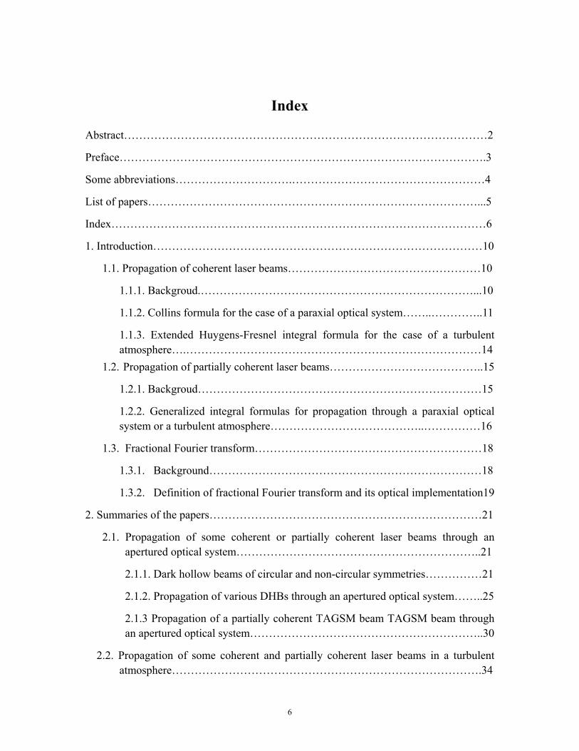
Fig. 9 Normalized irradiance distribution (contour graph) of a TAGSM beam at several

different propagation distances in a turbulent atmosphere (with 2 13 2/310nC m− −= ).

(a) z=0; (b) z=0.15km; (c) z=1km; (d) z=10km; (e) z=40km; (f) the free space case

(i.e., 2 0nC = ) with z=40km……………………………………………………...46

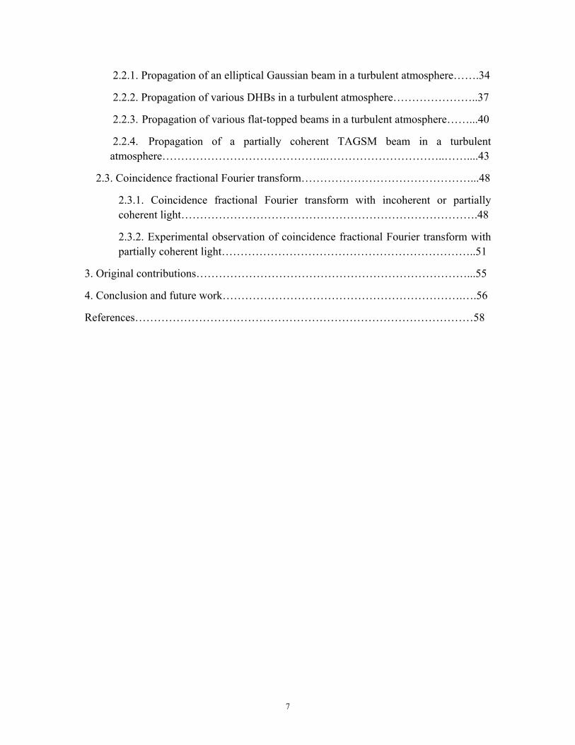
Fig. 10 Normalized irradiance distributions (contour graph) of TAGSM beams with

different initial levels of coherence and twist after propagating a fixed distance of

z=10km in various turbulent atmospheres. (a) ( ) ( )1 22 0.0166g mm− −=σ I ,

0µ = , 2 13 2/310nC m− −= ; (b) ( ) ( )1 22 0.0166g mm− −=σ I , 10.0002 ( )mmµ −= ,

2 13 2/310nC m− −= ; (c) ( ) ( )1 22g mm

− −=σ I , 0µ = , 2 13 2/310nC m− −= ; (d)

( ) ( )1 22 0.0166g mm− −=σ I , 0µ = , 2 14 2/310nC m− −= ……………………………..47

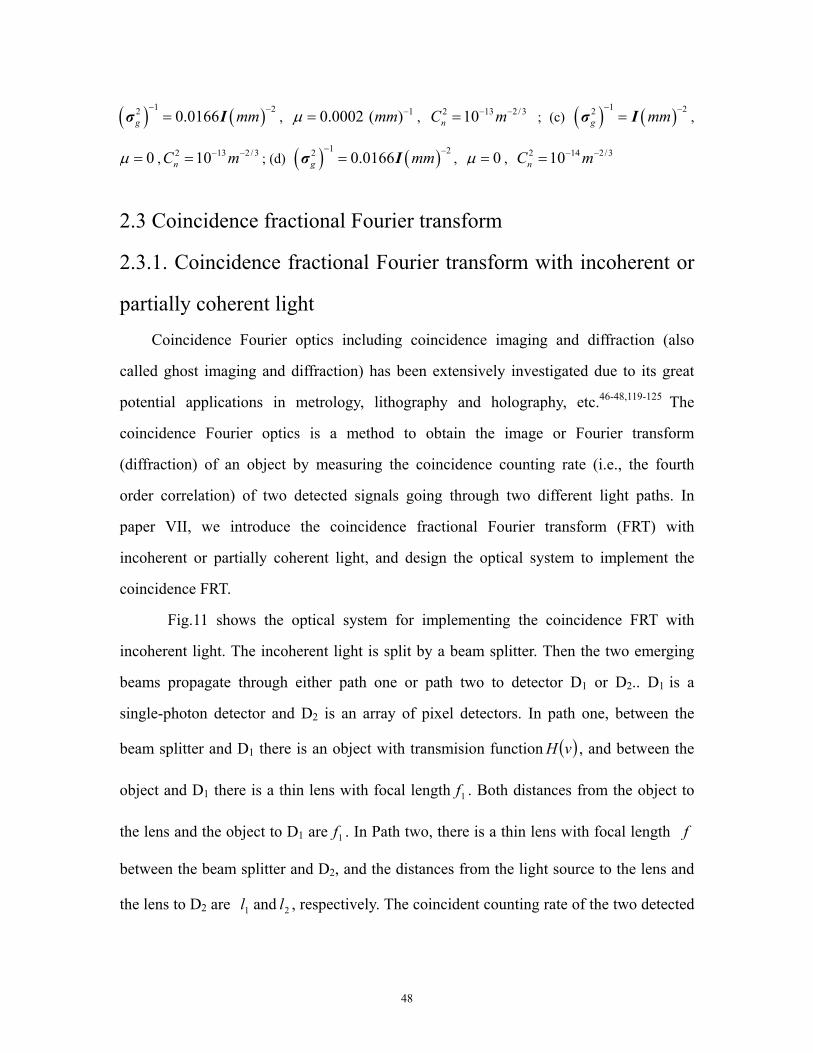
Fig.11 The optical system consisting of two thin lenses for implementing the coincidence

FRT with incoherent light………………………………………………………..49

Fig.12 Experimental setup for realizing a coincidence FRT with a partially coherent

light………………………………………………………………………………51

Fig.13 Experimental setup for measuring the coherence width of a partially coherent light

source…………………………………………………………………………….52

Fig.14 Square of the spectral degree of coherence [along ( 1 2x x− )] for a partially

coherent light source used in our experiment……………………………………53

Fig. 15 Experimental results of the coincidence FRT pattern for different fractional order

p for an object of double slits with a partially coherent beam ( 15g mσ µ= )……54

Fig. 16 Experimental results of the coincidence FRT pattern (with p=1) for an object of

double slits with partially coherent beams of different coherence width gσ ….…54

10

1. Introduction

1.1. Propagation of coherent laser beams

1.1.1. Backgroud In 1960, Maiman manufactured the first laser (ruby) in the world. Since then, lasers

have been extensively investigated both in theory and experiment, and have been widely

applied in many fields, such as free-space optical communications, material thermal

processing, inertial confinement fusion driven by lasers, laser biology and atomic

physics.1

The propagation and transformation of laser beams are the fundamental topics of

laser physics and laser applications.2 In the past decades, propagation of various laser

beams (including Gaussian beams, Laguerre-Gaussian beams, Hermite-Gaussian beams

Bessel Gaussian beams, and Hermite–sinusoidal-Gaussian beams, etc.) through a paraxial

optical system, free space or nonlinear media have been studied extensively.3-6 Many

methods such as the Wigner distribution function,7, 8 fast Fourier transform,9 Gaussian

beam decomposition,10 stable aggregate of flexible elements,11 and matrix and tensor

method,12-15 have been proposed to study the propagation and transformation of laser

beams.

Free-space optical (FSO) communication systems are becoming competitive in the

broadband access networks recently.16,17 Atmospheric turbulence plays a significant role

in FSO systems. Investigating the influences of atmospheric turbulence on the intensity

and spreading properties of a laser beam is necessary and important. Many researchers

have studied the spreading of laser beams in the turbulent atmosphere. Feizulin et al

studied the broadening of a spatially bounded laser beam.18 Young et al. studied the

spreading of a higher-order mode laser beam.19 The propagation and spreading of

11

partially coherent beams in a turbulent atmosphere have also been studied

extensively.20-24 Eyyuboğlu and Baykal investigated the properties of cosine-Gaussian,

cosh-Gaussian, Hermite–sinusoidal-Gaussian, Hermite-cosine-Gaussian and Hermite-

cosh-Gaussian laser beams in a turbulent atmosphere. 25-29 However, all these studies

treated axially symmetric beams or beams with profiles that can be expressed by

separable variables x and y. In a turbulent atmosphere the propagation of astigmatic

beams whose profile variables cannot be separated has not been investigated yet (except

in this thesis).

In the past several years, with the development of scientific technology, complicated

laser beams with special beam profiles such as a flat-topped beam,30-33 a dark hollow

beam34-36 and an astigmatic elliptical Gaussian beam37,38 are required in some

applications such as material thermal processing and atomic physics (atom guiding or

trapping). How to model these novel laser beams and analyze their propagation problems

have attracted more and more attentions. With these motivations, we propose several

theoretical models in this thesis to describe a dark hollow beam of circular or non-circular

symmetry, and investigate the propagation of various coherent laser beams through a

paraxial optical system or a turbulent atmosphere.

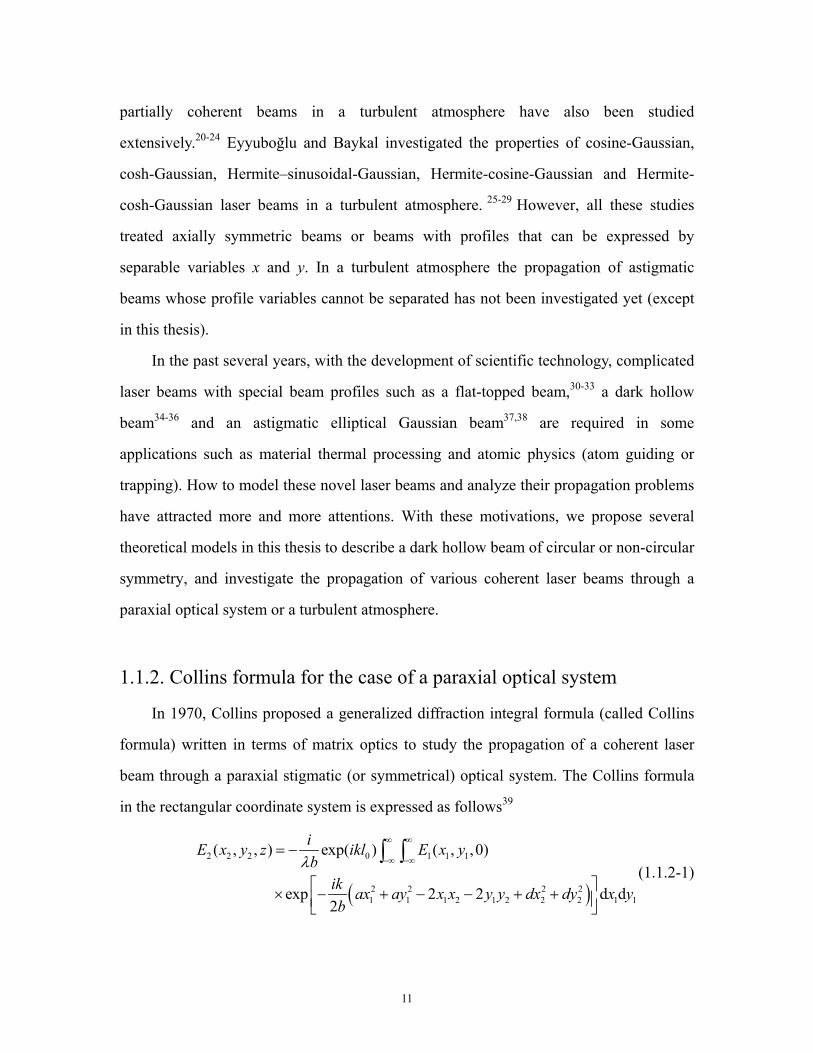
1.1.2. Collins formula for the case of a paraxial optical system

In 1970, Collins proposed a generalized diffraction integral formula (called Collins

formula) written in terms of matrix optics to study the propagation of a coherent laser

beam through a paraxial stigmatic (or symmetrical) optical system. The Collins formula

in the rectangular coordinate system is expressed as follows39

( )

2 2 2 0 1 1 1

2 2 2 21 1 1 2 1 2 2 2 1 1

( , , ) exp( ) ( , ,0)

exp 2 2 d d2

iE x y z ikl E x yb

ik ax ay x x y y dx dy x yb

λ∞ ∞

−∞ −∞= −

× − + − − + +

∫ ∫(1.1.2-1)

12

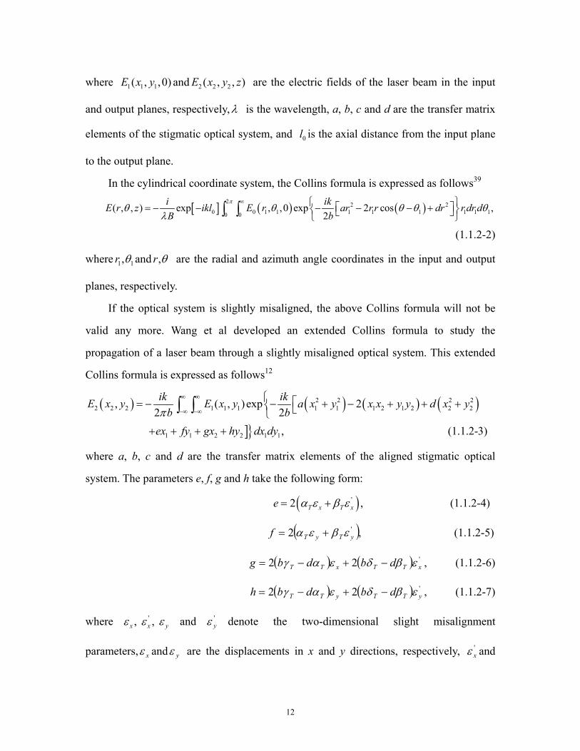
where 1 1 1( , ,0)E x y and 2 2 2( , , )E x y z are the electric fields of the laser beam in the input

and output planes, respectively,λ is the wavelength, a, b, c and d are the transfer matrix

elements of the stigmatic optical system, and 0l is the axial distance from the input plane

to the output plane.

In the cylindrical coordinate system, the Collins formula is expressed as follows39

[ ] ( ) ( )2 2 2

0 0 1 1 1 1 1 1 1 10 0( , , ) exp , ,0 exp 2 cos ,

2i ikE r z ikl E r ar r r dr r dr dB b

πθ θ θ θ θ

λ∞ = − − − − − + ∫ ∫

(1.1.2-2)

where 1 1,r θ and θ,r are the radial and azimuth angle coordinates in the input and output

planes, respectively.

If the optical system is slightly misaligned, the above Collins formula will not be

valid any more. Wang et al developed an extended Collins formula to study the

propagation of a laser beam through a slightly misaligned optical system. This extended

Collins formula is expressed as follows12

( ) ( ) ( ) ( )]}

2 2 2 22 2 2 1 1 1 1 1 1 2 1 2 2 2

1 1 2 2 1 1

, ( , ) exp 22 2

, (1.1.2-3)

ik ikE x y E x y a x y x x y y d x yb b

ex fy gx hy dx dyπ

∞ ∞

−∞ −∞

= − − + − + + + + + + +

∫ ∫

where a, b, c and d are the transfer matrix elements of the aligned stigmatic optical

system. The parameters e, f, g and h take the following form:

( )'2 ,T x T xe α ε β ε= + (1.1.2-4)

( ),2 'yTyTf εβεα += (1.1.2-5)

( ) ( ) '22 xTTxTT dbdbg εβδεαγ −+−= , (1.1.2-6)

( ) ( ) '22 yTTyTT dbdbh εβδεαγ −+−= , (1.1.2-7)

where ', , x x yε ε ε and 'yε denote the two-dimensional slight misalignment

parameters, xε and yε are the displacements in x and y directions, respectively, 'xε and

13

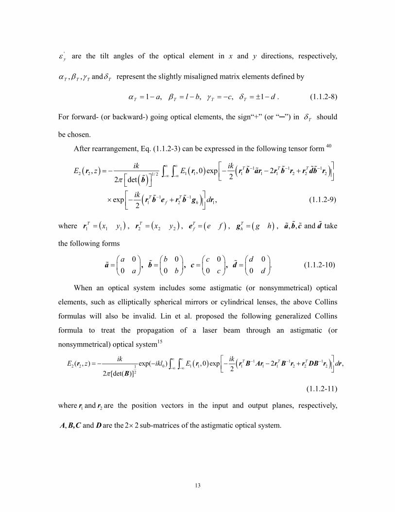
'yε are the tilt angles of the optical element in x and y directions, respectively,

TTT γβα ,, and Tδ represent the slightly misaligned matrix elements defined by

,1 aT −=α ,blT −=β ,cT −=γ dT −±= 1δ . (1.1.2-8)

For forward- (or backward-) going optical elements, the sign“+” (or “─”) in Tδ should

be chosen.

After rearrangement, Eq. (1.1.2-3) can be expressed in the following tensor form 40

( )( )

( ) ( )

( )

1 1 12 2 1 1 1 1 1 2 2 21/ 2

1 11 2 1

, ,0 exp 222 det

exp , (1.1.2-9)2

T T T

T Tf h

ik ikE z E

ik d

π

∞ ∞ − − −

−∞ −∞

− −

= − − − + × − +

∫ ∫r r r b ar r b r r db rb

r b e r b g r

where ( )111 yxT =r , ( )222 yxT =r , ( )Tf e f=e , ( )T

h g h=g , , ,a b c and d take

the following forms

0

0a

a

=

a , 0

0b

b

=

b , 0

0c

c

=

c , 0

.0d

d

=

d (1.1.2-10)

When an optical system includes some astigmatic (or nonsymmetrical) optical

elements, such as elliptically spherical mirrors or cylindrical lenses, the above Collins

formulas will also be invalid. Lin et al. proposed the following generalized Collins

formula to treat the propagation of a laser beam through an astigmatic (or

nonsymmetrical) optical system15

( ) ( )1 1 12 2 0 1 1 1 1 1 2 2 21

2

( , ) exp( ) ,0 exp 2 ,22 [det( )]

T T Tik ikE z ikl E dπ

∞ ∞ − − −

−∞ −∞

= − − − − + ∫ ∫r r r B Ar r B r r DB r rB

(1.1.2-11)

where 1r and 2r are the position vectors in the input and output planes, respectively,

DCB,A and , are the 2 2× sub-matrices of the astigmatic optical system.

14

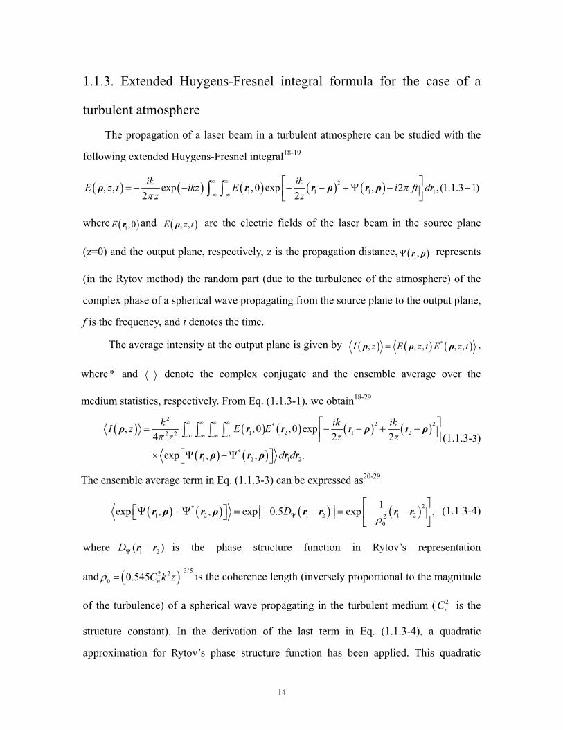
1.1.3. Extended Huygens-Fresnel integral formula for the case of a

turbulent atmosphere

The propagation of a laser beam in a turbulent atmosphere can be studied with the

following extended Huygens-Fresnel integral18-19

( ) ( ) ( ) ( ) ( )21 1 1 1, , exp ,0 exp , 2 , (1.1.3 1)

2 2ik ikE z t ikz E i ft d

z zπ

π∞ ∞

−∞ −∞

= − − − − +Ψ − − ∫ ∫ρ r r ρ r ρ r

where ( )1,0E r and ( ), ,E z tρ are the electric fields of the laser beam in the source plane

(z=0) and the output plane, respectively, z is the propagation distance, ( )1,Ψ r ρ represents

(in the Rytov method) the random part (due to the turbulence of the atmosphere) of the

complex phase of a spherical wave propagating from the source plane to the output plane,

f is the frequency, and t denotes the time.

The average intensity at the output plane is given by ( ) ( ) ( )*, , , , ,I z E z t E z t=ρ ρ ρ ,

where * and denote the complex conjugate and the ensemble average over the

medium statistics, respectively. From Eq. (1.1.3-1), we obtain18-29

( ) ( ) ( ) ( ) ( )

( ) ( )

22 2*

1 2 1 22 2

*1 2 1 2

, ,0 ,0 exp4 2 2

exp , , .

k ik ikI z E Ez z z

d d

π∞ ∞ ∞ ∞

−∞ −∞ −∞ −∞

= − − + −

× Ψ +Ψ

∫ ∫ ∫ ∫ρ r r r ρ r ρ

r ρ r ρ r r(1.1.3-3)

The ensemble average term in Eq. (1.1.3-3) can be expressed as20-29

( ) ( ) ( ) ( )2*1 2 1 2 1 22

0

1exp , , exp 0.5 exp ,DρΨ

Ψ +Ψ = − − = − −

r ρ r ρ r r r r (1.1.3-4)

where 1 2( )DΨ −r r is the phase structure function in Rytov’s representation

and ( ) 3/52 20 0.545 nC k zρ

−= is the coherence length (inversely proportional to the magnitude

of the turbulence) of a spherical wave propagating in the turbulent medium ( 2nC is the

structure constant). In the derivation of the last term in Eq. (1.1.3-4), a quadratic

approximation for Rytov’s phase structure function has been applied. This quadratic

15

approximation has been shown to be reliable in e.g. Ref. [20], and has been used widely

(see e.g. Refs. [20]-[29]).

1.2. Propagation of partially coherent laser beams

1.2.1. Backgroud A completely coherent laser beam does not exist in a strict sense. In a practical case,

most beams are partially coherent.41 In the past decades, especially since Wolf first found

that a partially coherent beam undergoes a spectral shift during its propagation in free

space, 42,43 partially coherent beams have been extensively studied both in experiment and

theory.41 Many interesting phenomena such as the spectral switch of partially coherent

light,44,45 reduced bit error rate in atmosphere communication,24 and ghost imaging and

diffraction with partially coherent light,46-48 superluminal propagation of partially

coherent pulses49 have been found to be related with the coherence of light. Partially

coherent light has been widely applied in practice, such as for optical projection, laser

scanning, improving the uniformity of the intensity distribution in inertial confinement

fusion and for the reduction of noise in photography.50,51

The Gaussian Schell-model (GSM) beam, one typical type of partially coherent

beams, plays an important role in the partial coherence theory. In 1975, Wolf and Carter

suggested the concept of the Gaussian quasi-homogeneous partially coherent source.52 A

bit later, the GSM source was introduced and fully developed by Wolf, Collet, Gori and

others,53-56 and has become known as the Wolf-Collett theorem in the literature. This idea

was extended by Friberg et al. to a GSM beam.57,58 A GSM beam has been successfully

demonstrated experimentally.59,60 In 1993, Simon and Mukunda introduced a new class of

partially coherent GSM beams incorporating a new twist phase quadratic in configuration

variables. This beam is called a twisted GSM (TGSM) beam.61-63 The twisted phase was

shown to be bounded in strength and can produce some nontrivial and observable effects

in the propagation of a GSM beam. TGSM beams have also been demonstrated

16

experimentally through an acousto-optic coherence control technique by Friberg et al.64

Propagation properties of GSM and TGSM beams have been extensively studied.65-68 The

commonly used method to study the propagation of GSM and TGSM beams is the

Wigner distribution function.61-63, 67-69 More recently, we have derived the tensor ABCD

law for the propagation of a TGSM beam through a paraxial optical system by using a

tensor method.70,71 In this thesis, we study the propagation of a TGSM beam through an

apertured paraxial optical system or a turbulent atmosphere by using the tensor method.

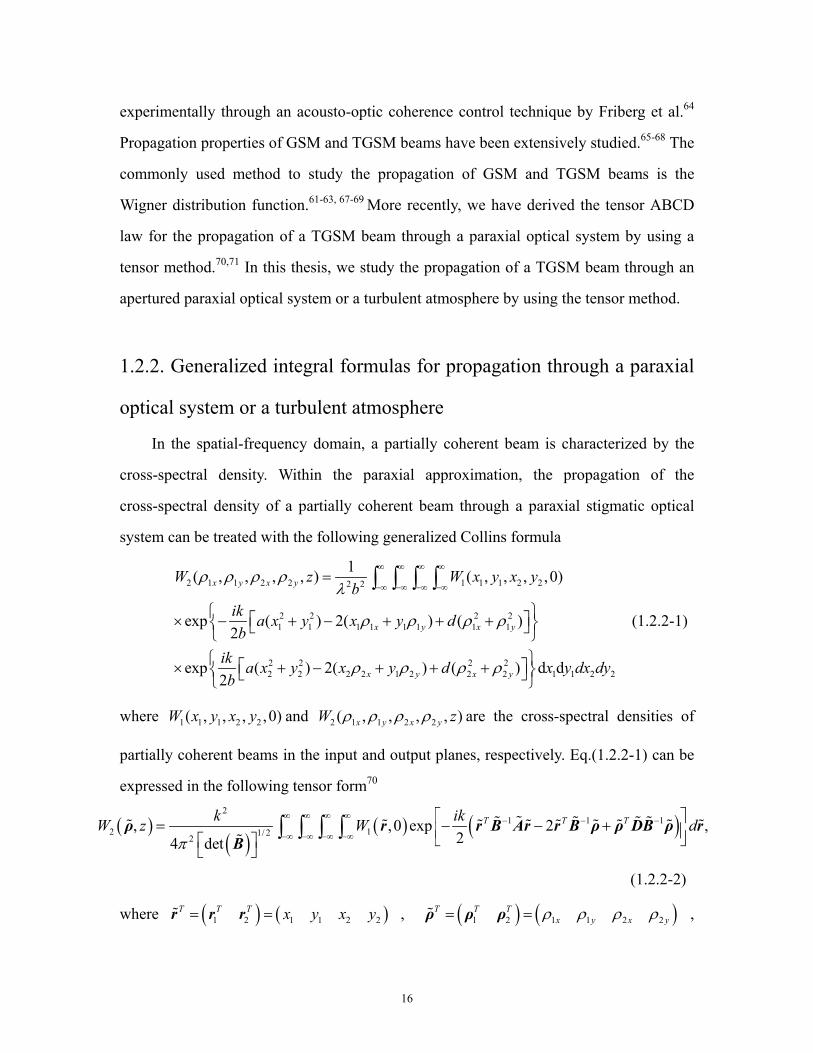
1.2.2. Generalized integral formulas for propagation through a paraxial

optical system or a turbulent atmosphere

In the spatial-frequency domain, a partially coherent beam is characterized by the

cross-spectral density. Within the paraxial approximation, the propagation of the

cross-spectral density of a partially coherent beam through a paraxial stigmatic optical

system can be treated with the following generalized Collins formula

2 1 1 2 2 1 1 1 2 22 2

2 2 2 21 1 1 1 1 1 1 1

2 2 2 22 2 2 2 1 2 2 2 1 1 2 2

1( , , , , ) ( , , , ,0)

exp ( ) 2( ) ( )2

exp ( ) 2( ) ( ) d d2

x y x y

x y x y

x y x y

W z W x y x yb

ik a x y x y db

ik a x y x y d x y dx dyb

ρ ρ ρ ρλ

ρ ρ ρ ρ

ρ ρ ρ ρ

∞ ∞ ∞ ∞

−∞ −∞ −∞ −∞=

× − + − + + + × + − + + +

∫ ∫ ∫ ∫

(1.2.2-1)

where 1 1 1 2 2( , , , ,0)W x y x y and 2 1 1 2 2( , , , , )x y x yW zρ ρ ρ ρ are the cross-spectral densities of

partially coherent beams in the input and output planes, respectively. Eq.(1.2.2-1) can be

expressed in the following tensor form70

( )( )

( ) ( )2

1 1 12 11/ 22

, ,0 exp 2 ,24 det

T T Tk ikW z W dπ

∞ ∞ ∞ ∞ − − −

−∞ −∞ −∞ −∞

= − − +

∫ ∫ ∫ ∫ρ r r B Ar r B ρ ρ DB ρ rB

(1.2.2-2)

where ( ) ( )1 2 1 1 2 2T T T x y x y= =r r r , ( ) ( )1 2 1 1 2 2

T T Tx y x yρ ρ ρ ρ= =ρ ρ ρ ,

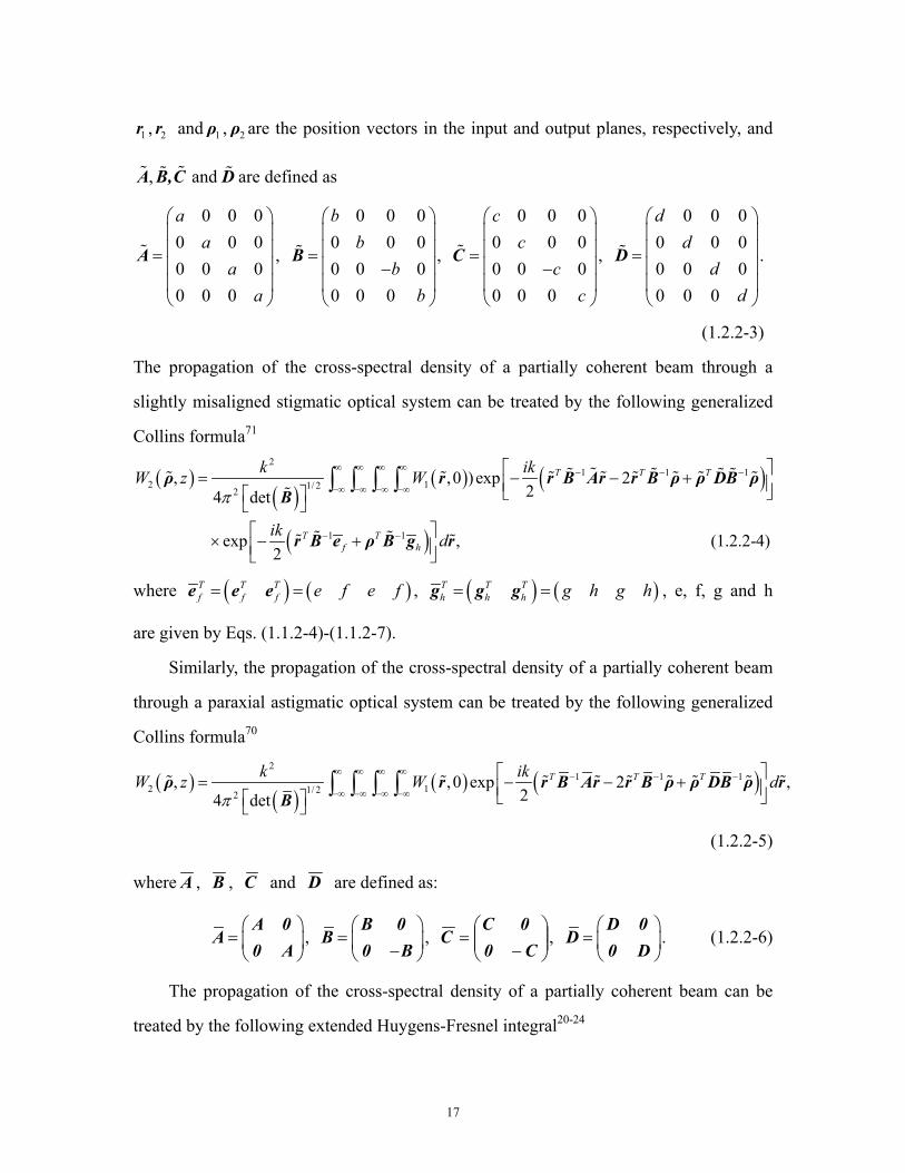
17

1r , 2r and 1ρ , 2ρ are the position vectors in the input and output planes, respectively, and

, and A B,C D are defined as

0 0 00 0 00 0 00 0 0

aa

aa

=

A ,

0 0 00 0 00 0 00 0 0

bb

bb

= −

B ,

0 0 00 0 00 0 00 0 0

cc

cc

= −

C ,

0 0 00 0 00 0 00 0 0

dd

dd

=

D .

(1.2.2-3)

The propagation of the cross-spectral density of a partially coherent beam through a

slightly misaligned stigmatic optical system can be treated by the following generalized

Collins formula71

( )( )

( ) ( )

( )

21 1 1

2 11/ 22

1 1

, ,0 )exp 224 det

exp , 2

T T T

T Tf h

k ikW z W

ik d

π

∞ ∞ ∞ ∞ − − −

−∞ −∞ −∞ −∞

− −

= − − + × − +

∫ ∫ ∫ ∫ρ r r B Ar r B ρ ρ DB ρB

r B e ρ B g r (1.2.2-4)

where ( ) ( )T T Tf f f e f e f= =e e e , ( ) ( )T T T

h h h g h g h= =g g g , e, f, g and h

are given by Eqs. (1.1.2-4)-(1.1.2-7).

Similarly, the propagation of the cross-spectral density of a partially coherent beam

through a paraxial astigmatic optical system can be treated by the following generalized

Collins formula70

( )( )

( ) ( )2

1 1 12 11/ 22

, , 0 exp 2 ,24 det

T T Tk ikW z W dπ

∞ ∞ ∞ ∞ − − −

−∞ −∞ −∞ −∞

= − − + ∫ ∫ ∫ ∫ρ r r B Ar r B ρ ρ DB ρ r

B

(1.2.2-5)

where A , B , C and D are defined as:

=

A 0A

0 A,

= −

B 0B

0 B,

−

=C0

0CC ,

=

D 0D

0 D. (1.2.2-6)

The propagation of the cross-spectral density of a partially coherent beam can be

treated by the following extended Huygens-Fresnel integral20-24

18

( ) ( )

( ) ( )

22 2

2 1 2 1 1 2 1 1 2 22 2

*1 1 2 2 1 2

( , , ) ( , ,0)exp4 2 2

exp , , , , , (1.2.2 7)

k ik ikW z Wz z z

z z d d

π∞ ∞ ∞ ∞

−∞ −∞ −∞ −∞

= − − + −

× Ψ +Ψ −

∫ ∫ ∫ ∫ρ ρ r r r ρ r ρ

r ρ r ρ r r

where 1 1 2( , ,0)W r r and 2 1 2 ( , , )W zρ ρ are the cross-spectral densities in the input and

output planes, respectively. Like in Section 1.1.3, in the Rytov method ( )1 1,Ψ r ρ

represents the random part (due to the turbulence of the atmosphere) of the complex

phase of a spherical wave propagating from the source plane to the output plane, and “<

>” denotes the average over the ensemble of the turbulent medium. Under a quadratic

approximation, the ensemble average term in Eq. (1.2.2-7) can be expressed as follows 20-24

( ) ( ) ( ) ( )2*1 1 2 2 1 2 1 22

0

1exp , , exp 0.5 exp ,DρΨ

Ψ +Ψ = − − = − −

r ρ r ρ r r r r (1.2.2-8)

where 1 2( )DΨ −r r and 0ρ take the same form as in Section 1.1.3.

1.3. Fractional Fourier transform

1.3.1. Background

In 1980, the concept of fractional Fourier transform (FRT) was proposed by

Namias as the generalization of the conventional Fourier transform, and was used as a

mathematical tool for solving some theoretical physical problems.72 McBride and Kerr

developed Namias’ definition and made it more rigorous.73 In 1993, Ozaktas, Mendlovic

and Lohmann introduced FRT into optics and designed several optical systems such as

some gradient-index fiber and lens system to achieve FRT.74-76 Since then, FRT has been

extensively investigated and found wide applications in information processing, motion

detection and analysis, holographic data storage, optical neural networking, optical image

encryption, beam analysis, beam smoothing and beam shaping, etc.77-79 Several devices

19

for the manipulation of optical beams based on the FRT have been proposed recently. The

FRT is applied to a / 2π converter, which is used to obtain focused Laguerre-Gaussian

beams from Hermite-Gaussian radiation modes.80 The design of a diffractive optical

element for beam smoothing in the fractional Fourier domain was proposed in Ref. [81].

Recently, the discrete FRT,82 scaled FRT,83 the fractional Hilbert transform,84 Fractional

Hankel transform 85 and multifractional correlation 86 have also been defined. In this

thesis, we introduce the concept of the coincidence FRT with an incoherent or partially

coherent beam, design the optical system for implementing the coincidence FRT, and

demonstrate experimentally the coincidence FRT with a partially coherent beam.

1.3.2 Definition of the fractional Fourier transform and its optical

implementation

Here we introduce briefly Lohmann’s definition of FRT. Lohmann defined the FRT

as follows74

( ) ( ) ( ) 1211

22

21

110

12 sin

2tan

expsin

dxxxfixx

fixE

fixE p ∫∫

++−−=

ϕλπ

ϕλπ

ϕλ, (1.3.2-1)

where ( )0 1E x and ( )2pE x are the fields in the input plane and the FRT plane, respectively,

ef is the “standard focal length”, and φ is defined by 2πφ p

= with p the fractional

order of the FRT. The value of p can be any arbitrary real number. When p takes the value

of 14 +n (n being any integer), the fractional Fourier field )( 2xE p reduces to the

traditional Fourier field in the plane of the focal plane of the lens with a focal length ef .

The factor 1/ sini fλ ϕ− in Eq. (1.3.2-1) ensures the energy conservation after the FRT

transform.

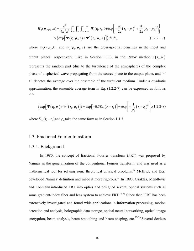
Many optical systems have been proposed to realize the FRT. Fig. 1 shows two

20

types of optical systems proposed by Lohmann for performing the FRT.

()

(a) (b)

Fig. 1 Optical system for performing the FRT. (a) one-lens system; (b) two-lens system.

Input plane

Input plane

( )2pE x( )1E x

φsin/f

( )2/tan φf ( )2/tan φf

( )2/tan/ φf( )2/tan/ φf

2( )pE x1( )E x

φsinf

FRT plane

FRT plane

21

2. Summaries of the Papers In this part the papers included in this thesis are summarized. These papers can be

divided into the following three categories: (1) Propagation of some coherent or partially

coherent beams through an apertured paraxial optical system (Papers I and III); (2)

Propagation of some coherent or partially coherent beams in a turbulent atmosphere

(Papers II and IV-VI); (III) Coincidence fractional Fourier transform with an incoherent

or partially coherent beam (Papers VII and VIII). In the first category, some theoretical

models for describing dark hollow beam (DHB) of circular or non-circular symmetry are

proposed, and analytical formulas for various DHBs and a partially coherent TAGSM

beam through an apertured paraxial optical system are derived. In the second category,

analytical formulas for an elliptical Gaussian beam (EGB), various DHBs, flat-topped

beams and a TAGSM beam propagating in a turbulent atmosphere are derived, and their

propagation properties are investigated. In the third category, coincidence FRT with an

incoherent or partially coherent beam is introduced, and is demonstrated experimentally

with a partially coherent beam.

2.1 Propagation of some coherent or partially coherent laser beams

through an apertured optical system

2.1.1 Dark hollow beams of circular or non-circular symmetries

Recently, dark-hollow beams (DHBs) have attracted more and more attention

because of their wide applications in modern optics and atomic optics.34 Various

techniques such as geometrical optical method, mode conversion, optical holography,

transverse-mode selection, hollow-fiber method, computer-generated holography and

nonlinear optical method have been used to generate DHBs.87-90 DHBs have been used in

atom guiding and trapping.35, 36 There exist several theoretical models to describe DHBs,

22

such as the *01TEM beam and the higher-order Bessel beam.35, 5, 91 In most of the literature,

the DHBs have been assumed to be of circular symmetry. However, in a practical case,

most DHBs are of non-circular symmetry. In Papers I and II, we propose several

theoretical models to describe DHBs of circular, elliptical and rectangular symmetries.

To describe a DHB of circular symmetry, we express its electric field at 0=z as

follows:

( )2 2

1 11 0 2 2

0 0

,0 expn

nr rE r Gw w

= −

, ,...2,1,0=n , (2.1.1-1)

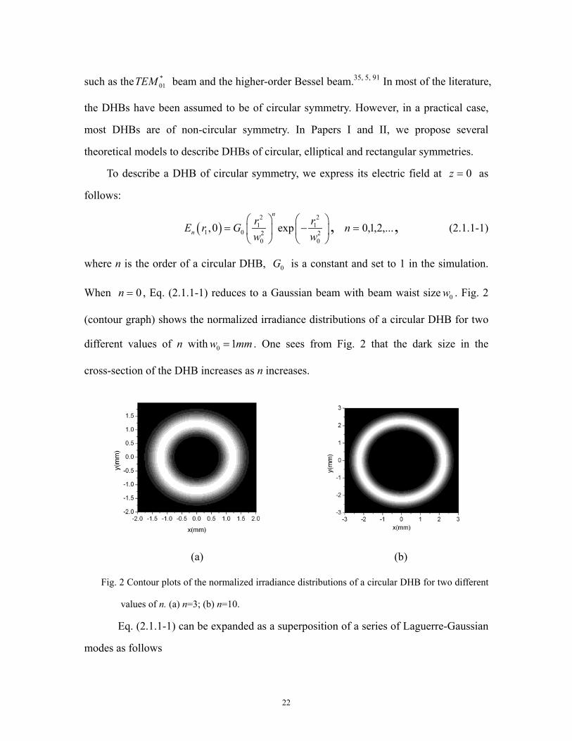
where n is the order of a circular DHB, 0G is a constant and set to 1 in the simulation.

When 0=n , Eq. (2.1.1-1) reduces to a Gaussian beam with beam waist size 0w . Fig. 2

(contour graph) shows the normalized irradiance distributions of a circular DHB for two

different values of n with 0 1w mm= . One sees from Fig. 2 that the dark size in the

cross-section of the DHB increases as n increases.

(a) (b)

Fig. 2 Contour plots of the normalized irradiance distributions of a circular DHB for two different

values of n. (a) n=3; (b) n=10.

Eq. (2.1.1-1) can be expanded as a superposition of a series of Laguerre-Gaussian

modes as follows

23

( ) ( )2 2

1 11 0 2 2

0 0 0

!,0 1 2 exp2

nm

n mnm

n r rnE r G Lm w w=

= − −

∑ , (2.1.1-2)

where nm

denotes a binomial coefficient and mL is the mth Laguerre polynomial.

To describe a DHB of elliptical symmetry, we express its electric field at 0=z in a

tensor form as follows:

1 11 0 1 1 1 1 1 1( ,0) exp , 0,1,2,3.........

2 2

nT T

nik ikE G n− − = − =

r r Q r r Q r (2.1.1-3)

where r is the position vector given by 1 ( )T x y=r , n is the order of an elliptical DHB,

11−Q is a 22× complex curvature tensor (a generalization of 1/q ) given by:

1 10 01

1 1 10 0

xx xy

xy yy

q qq q

− −−

− −

=

Q , (2.1.1-4)

where 20 01/ 2 /xx xq i kw= − , 2

0 01/ 2 /xy xyq i kw= − , 20 01/ 2 /yy yq i kw= − , 0 0 and x yw w are the

beam waists along x- and y-directions, respectively, xyw0 is the cross element related

with the orientation of the beam spot. Eq. (2.1.1-3) is called the n-th order elliptical DHB.

When 0=n , Eq. (2.1.1-3) reduces to the elliptical Gaussian beam with complex curvature

tensor 11−Q . Similarly, the elliptical DHB can be expressed as a superposition of a series of

elliptical Hermite-Gaussian modes.92

Recently, Mei et al proposed a new theoretical model to describe a circular DHB by

expressing its electric field as a superposition of a series of Gaussian beams.93 As an

extension of their model, we propose in Paper II another model to describe a DHB of

elliptical symmetry by expressing its electric field at z=0 as the following superposition

of a series of elliptical Gaussian beams

( ) ( ) 11 1

1 1 1 1 1 1 11

1,0 exp exp

2 2

nNT T

N n npn

N ik ikEnN

−− −

=

− = − − − ∑r r Q r r Q r , (2.1.1-5)

24

where 11n−Q and 1

1np−Q are given by

2 20 01

1

2 20 0

2 2

2 2x xy

n

xy y

n nikw ikw

n nikw ikw

−

=

Q , 2 20 01

1

2 20 0

2 2

2 2x xy

np

xy y

n nipkw ikpw

n nikpw ikpw

−

=

Q , (2.1.1-6)

and Nn

denotes a binomial coefficient, N is the order of a circular dark hollow beam,

and p is a real positive parameter satisfying 1p < . We can adjust the central dark size of

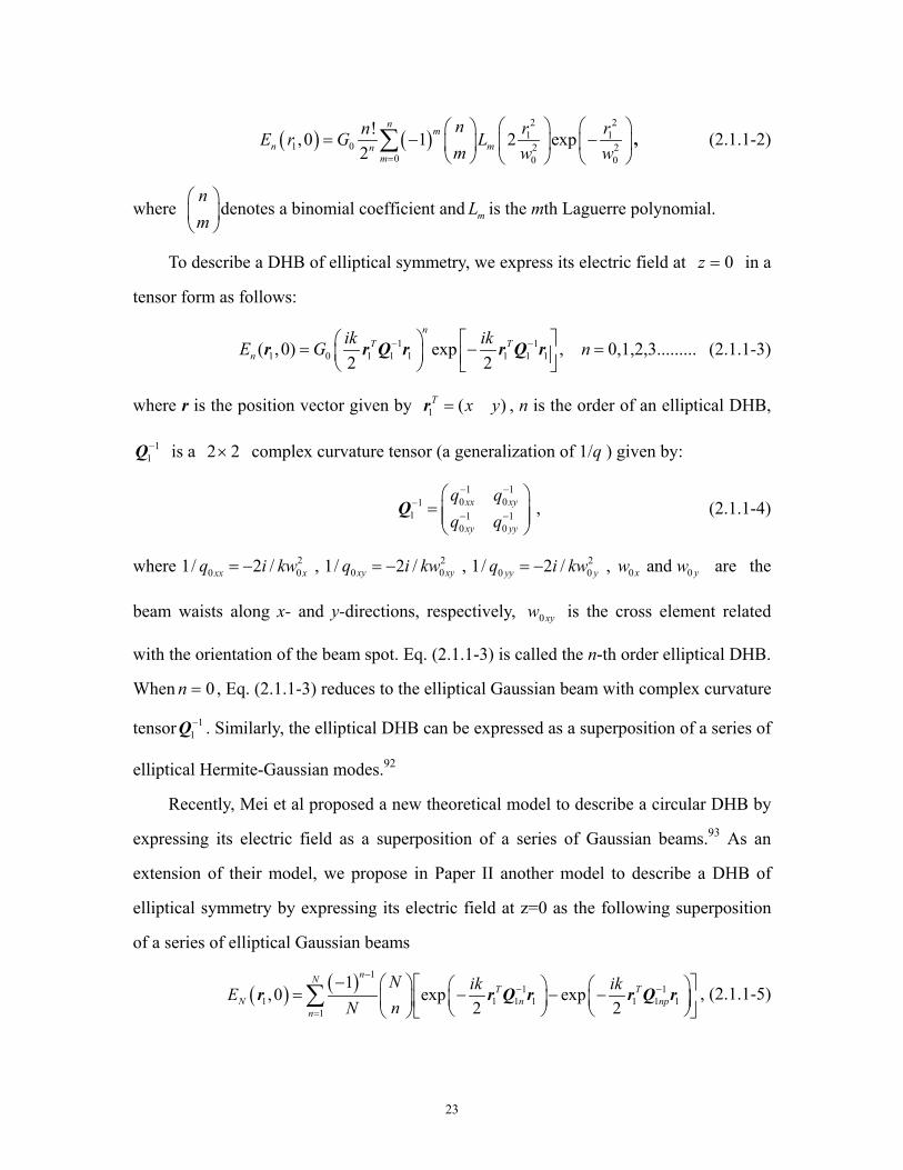
the DHB by varying p. Thus, p can be called a dark-size-adjusting parameter. Fig. 3

(contour graph) shows the normalized irradiance distributions of an elliptical DHB for

two different sets of yx ww 00 , and xyw0 with N=10 and p=0.9.

(a) (b)

Fig. 3 Contour plots of the normalized intensity distributions of an elliptical DHB for two

different sets of yx ww 00 , and xyw0 with N=10 and p=0.9. (a) 0 1xw mm= , 0 2yw mm= ,

0 2xyw mm= ; (b) 0 2xw mm= , 0 1yw mm= , 0 2xyw mm= .

Similarly, we also express the field of a DHB of rectangular symmetry at z=0 as the

following finite sum of elliptical Gaussian beams in Paper II

( ) ( ) 1 11 1 1 1 1 1

1 1

1, ,0 exp exp , (2.1.1-7)

2 2

h nH NT T

HN hn hnph n

H N ik ikE x yh nHN

+− −

= =

− = − − − ∑∑ r Q r r Q r

where H and N indicate the orders of a rectangular DHB and

25

201

120

2 0

20x

hn

y

hikw

nikw

−

=

Q , 201

120

2 0

20x

hnp

y

hikpw

nikpw

−

=

Q . (2.1.1-8)

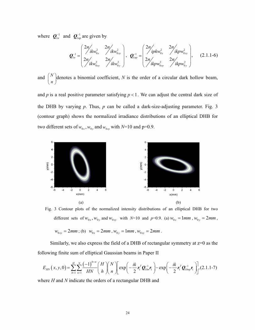
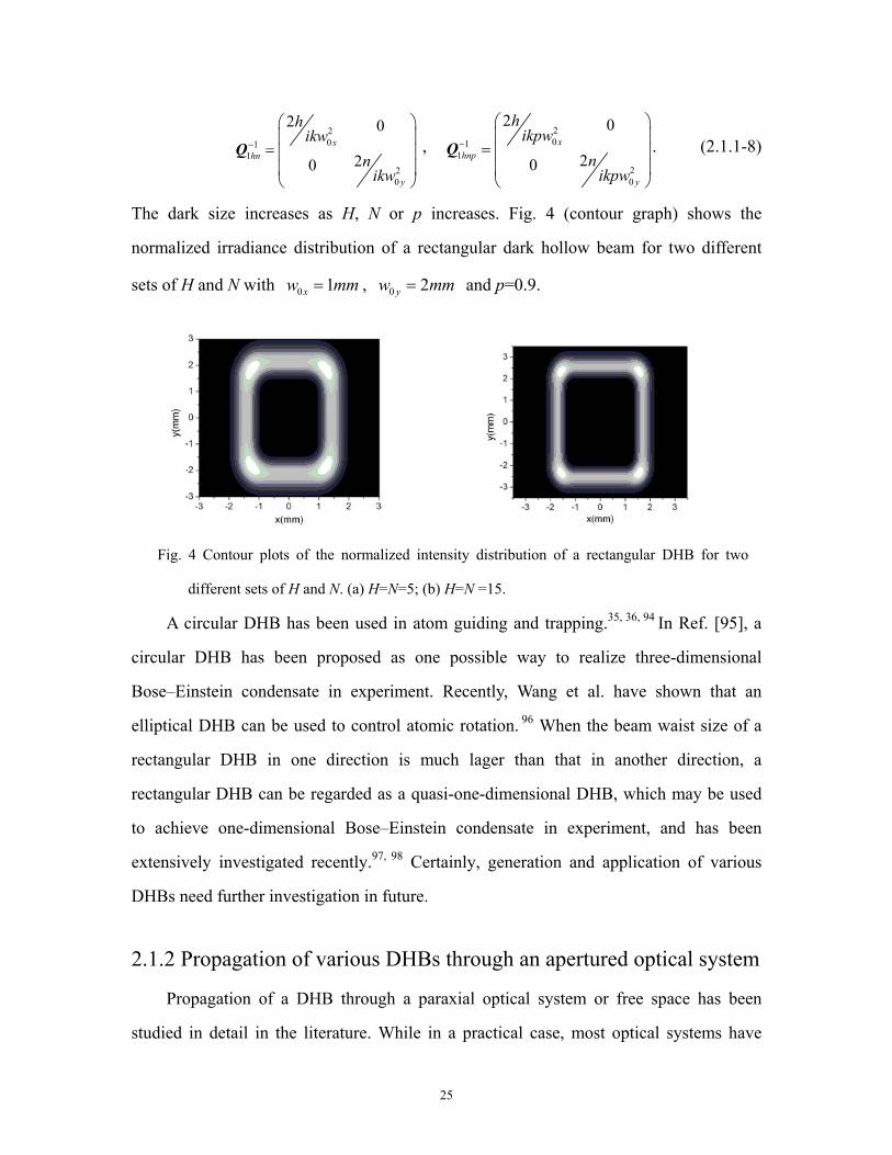
The dark size increases as H, N or p increases. Fig. 4 (contour graph) shows the

normalized irradiance distribution of a rectangular dark hollow beam for two different

sets of H and N with 0 1xw mm= , 0 2yw mm= and p=0.9.

Fig. 4 Contour plots of the normalized intensity distribution of a rectangular DHB for two

different sets of H and N. (a) H=N=5; (b) H=N =15.

A circular DHB has been used in atom guiding and trapping.35, 36, 94 In Ref. [95], a

circular DHB has been proposed as one possible way to realize three-dimensional

Bose–Einstein condensate in experiment. Recently, Wang et al. have shown that an

elliptical DHB can be used to control atomic rotation. 96 When the beam waist size of a

rectangular DHB in one direction is much lager than that in another direction, a

rectangular DHB can be regarded as a quasi-one-dimensional DHB, which may be used

to achieve one-dimensional Bose–Einstein condensate in experiment, and has been

extensively investigated recently.97, 98 Certainly, generation and application of various

DHBs need further investigation in future.

2.1.2 Propagation of various DHBs through an apertured optical system

Propagation of a DHB through a paraxial optical system or free space has been

studied in detail in the literature. While in a practical case, most optical systems have

26

finite size and are apertured. Thus it is necessary to take the aperture effect into

consideration. In fact, many interesting phenomena of light propagation through an

apetured paraxial optical system, such as focal shift and switch, spectral shift and switch,

have been reported.99,100, 44 In Paper I, we derive the analytical propagation formula for a

DHB of circular or non-circular symmetry through an apertured optical system.

In a cylindrical coordinate system, the propagation of a coherent laser beam through

a cirucular apertured ABCD optical system can be treated by the following Collins

formula (cf. Eq. (1.1.2-2)):

[ ] ( ) ( )12 2 20 0 1 1 1 1 1 1 10 0

( , ) exp ,0 exp 2 cos ,2

ai ikE r z ikl E r ar r r dr r dr dB b

πθ θ θ

λ = − − − − + ∫ ∫

(2.1.2-1)

where 1a denotes the radius of the aperture.

By introducing the following circular aperture function

( ) 1 11

1 1

1, , (2.1.2-2)

0, ,r a

H rr a

≤= >

We can rewrite Eq. (2.1.2-1) as

[ ] ( ) ( ) ( )2 2 2

0 0 1 1 1 1 1 1 1 10 0( , ) exp ,0 exp 2 cos ,

2i ikE r z ikl E r H r ar r r dr r dr dB b

πθ θ θ

λ∞ = − − − − + ∫ ∫

(2.1.2-3)

The aperture function in Eq. (2.1.2-2) can be expanded as the following finite sum of

complex Gaussian functions101, 102

( ) 21 12

1 1

expM

mm

m

BH r A ra=

= −

∑ , (2.1.2-4)

where mA and mB are the expansion and Gaussian coefficients, which can be obtained

directly from numerical optimization.101, 102 A table for mA and mB can be found in Refs.

[101] and [102]. Our numerical results show that the simulation accuracy improves as M

27

increases. Then substituting Eqs. (2.1.1-1) and (2.1.2-4) into Eq.(2.1.2-3), we obtain

(after some straightforward integration) the following approximate analytical formula for

a circular DHB through a circular apertured ABCD optical system

( )12

002 2 2

10 0 1

2 2

2 2 2 20 1 0 1

! 1( , ) exp exp2 2 2

2 2 exp .1 1

2 2

nMm

n mnm

nm m

ikG n Bikdr ikaE r z ikl Abw b w b a

kr krb bL

B Bika ikaw b a w b a

− −

=

= − − + +

−

+ + + +

∑

(2.1.2-5)

Substituting Eqs. (2.1.1-2) and (2.1.2-4) into Eq.(2.1.2-3), we obtain (after integration)

the following equivalent approximate analytical formula for a circular DHB through a

circular apertured ABCD optical system

( ) ( )21 00

0 10 1

21 0

22 2 2

0 1

22 2

2 02 20 1 0 1

2!( , ) exp 1

2 2

2

exp2 22 2

2

n

mn M

pn m nn

p m m

m

pm m

B B BAn ika qG nE r z ikl Ap B B BA

ika q

B DDik C rq ika k rL

B BB BB ikAA w Bq ika w a B

+= =

+ − = − −

+ +

+ +

−

+ + − +

∑∑

2 .

(2.1.2-6)

After some rearrangement, the circular aperture function given by Eq. (2.1.2-2) can

be expressed in the following tensor form

( )1 1 11

exp2

MT

m mm

ikH A=

= −

∑r r R r , (2.1.2-7)

with ( )1 1 1T x y=r and

21

1 020 1

mm

Bika

=

R . (2.1.2-8)

Then substituting Eqs. (2.1.1-3) and (2.1.2-7) into Eq. (1.1.2-11), we obtain (after some

vector integration and tensor operation) the following approximate analytical formula for

28

an elliptical DHB propagating through an apertured astigmatic ABCD optical system

( ) ( )

( ) ( ){

1/ 21 12 0 0 1 2 2 23

1 0

1/ 21 11 1 2 1 1

12 1

(2 )!( , ) exp det exp2 ( )!(2 )! 2

1 2 det 1 2 / det

M nTm

n m mnm p

p

p

T

An ikE z G ikl n p p

/ H

ik

−− −

= =

−− −

−

= − + + − −

× − + + − + +

× +

∑∑

m m

r A BQ BR r Q r

B AQ R Q I B AQ R Q I

r A B Q( ) ( )1 1

1 1 2 , (2.1.2-9)T

m

− − + + mR AQ B I + R Q r

where ( ) ( ) 11 1 12 1 1m m m

−− − − = + + + + Q C D Q R A B Q R , I is a 2 2× unit matrix.

Similarly, we can obtain the following approximate analytical formula for an elliptical

DHB propagating through an apertured slightly misaligned ABCD optical system

( ) ( )

( )

1/ 21 1

2 0 0 1 231 0

11 1 1 1 12 2 2 2 1 1

(2 )!( , ) exp det exp2 ( )!(2 )! 2

exp exp exp2 2 8

M nTm

n m gnm p

T T T T Tm m f f

An ikE z G ikl n p p

ik ik ik

−− −

= =

−− − − − −

= − + + − −

× − − + + + +

∑∑r a bQ bR r b g

r Q r r b a bQ bR e e b a bQ( )

( ) ( ){( ) ( ) ( ) ( )

1/ 21 1

1 1 2 1 1

1 112 1 1 1 2

1 2 det 1 2 / det

/ 2 / 2 , (2.1.2-11)

m f

p

p

TT

f m f

/ H

ik

−− −

− −−

× − + + − + +

× − + + + −

m m

m

bR e

b aQ R Q I b aQ R Q I

r e a b Q R aQ b I + R Q r e

where ( ) ( ) 11 1 12 1 1m m m

−− − − = + + + + Q c d Q R a b Q R .

When the aperture is rectangular, the aperture function can be expressed as follows

( ) 1 1 1 11 1

1 1 1 1

1, , ,, (2.1.2-12)

0, ,x a y b

H x yx a y b

≤ ≤= > >

where 12a and 12b denote the aperture widths in x- and y- directions, respectively. Eq.

(2.1.2-12) can also be expanded as the following finite sum of complex Gaussian

functions

( ) 2 21 1 1 12 2

1 11 1

, exp expM J

jmm j

m j

BBH x y A x A ya b= =

= − −

∑ ∑ , (2.1.2-13)

where mA , mB , jA and jB are the expansion and Gaussian coefficients. After some

rearrangement, Eq. (2.1.2-13) can be expressed in the following tensor form

29

( )1 1 11 1

exp2

M JT

m j mjm j

ikH A A= =

= −

∑∑r r R r , (2.1.2-14)

with

21

21

2 0

20

m

mjj

Bika

Bikb

=

R . (2.1.2-15)

Substituting Eqs. (2.1.1-3) and (2.1.2-14) into Eq. (1.1.2-11), we obtain (after integration)

the following approximate analytical formula for an elliptical DHB through a rectangular

apertured astigmatic ABCD optical system

( ) ( )

( ) ( ){

1/ 21 12 0 0 1 2 2 23

1 1 0

1/ 21 11 1 2 1 1

(2 )!( , ) exp det exp2 ( )!(2 )! 2

1 2 det 1 2 / det

M J nm j T

n mj mjnm j p

p

mj p mj

A An ikE z G ikl n p p

/ H

i

−− −

= = =

−− −

= − + + − −

× − + + − + +

×

∑∑∑r A BQ BR r Q r

B AQ R Q I B AQ R Q I

( ) ( )1 112 1 1 1 2 , (2.1.2-16)

TTmj mjk

− −− + + + r A B Q R AQ B I + R Q r

with ( ) ( ) 11 1 12 1 1mj mj mj

−− − − = + + + + Q C D Q R A B Q R . Similarly, we can obtain the

following approximate analytical formula for an elliptical DHB through a rectangular

apertured slightly misaligned ABCD optical system

( ) ( )

( )

1/ 21 1

2 0 0 1 231 1 0

11 1 12 2 2 2 1

(2 )!( , ) exp det exp2 ( )!(2 )! 2

exp exp exp2 2 8

M J nm j T

n mj gnm j p

T T T Tmj mj f f

A An ikE z G ikln p p

ik ik ik

−− −

= = =

−− − − −

= − + + − −

× − − + +

∑∑∑r a bQ bR r b g

r Q r r b a bQ bR e e b ( )

( ) ( ){( ) ( ) ( ) ( )

1 11

1/ 21 1

1 1 2 1 1

1 112 1 1 1 2

1 2 det 1 2 / det

/ 2 / 2 , (2.1.2-17)

Tmj f

p

mj p mj

TT

f mj mj f

/ H

ik

−

−− −

− −−

+ +

× − + + − + +

× − + + + −

a bQ bR e

b aQ R Q I b aQ R Q I

r e a b Q R aQ b I + R Q r e

with ( ) ( ) 11 1 12 1 1mj mj mj

−− − − = + + + + Q c d Q R a b Q R .

Under the condition of 1a − > ∞ and 1b − > ∞ , the approximate formulas derived

above reduce to the formulas for a DHB of circular or elliptical symmetry propagating

30

through an unapertured ABCD optical system. Numerical results of Paper I clearly show

that the results calculated by the above approximate analytical formulas are in a good

agreement with those calculated by using the numerical integral calculation. Through a

similar derivation, we can easily obtain the approximate analytical formula for a

rectangular DHB through an apertured ABCD optical system.

2.1.3 Propagation of a partially coherent TAGSM beam through an

apertured astigmatic optical system

A partially coherent twisted anisotropic Gaussian Schell-model (TAGSM) beam is

a typical model for describing a general astigmatic partially coherent beam.61-63 TAGSM

beams have been widely studied both theoretically and experimentally.64-68 In all the

previous research works about the propagation of a TAGSM beam through a paraxial

optical system, the optical system has been assumed to be unapertured (ideal case). In a

practical case, most optical systems are apertured. Thus it is necessary to study the

propagation of a TAGSM beam through an apertured optical system. While up to now,

the propagation of partially coherent light through an apertured optical system is

calculated through the time-consuming numerical integration. There is no suitable

analytical method for treating the propagation of a partially coherent beam through such a

system. In Paper III, we derive an approximate analytical formula for a TAGSM beam

propagating through an apertured astigmatic optical system by use of a tensor method.

The cross-spectral density of a TAGSM beam at z=0 can be expressed in the

following tensor form 70

11 0 1( ,0) exp

2TikW G − = −

r r M r , (2.1.3-1)

where ( )1 1 2 2T x y x y=r , 1

1−M is a 44× partially coherent complex curvature

tensor,

31

( ) ( ) ( )

( ) ( ) ( )

1 1 11 2 2 2

11

1 1 12 1 2 2

2

2

I g g

Tg I g

i i ik k k

i i ik k k

µ

µ

− − −−

−

− − −−

− − + = + − − −

R σ σ σ JM

σ J R σ σ, (2.1.3-2)

where 2Iσ is a 2 2× transverse spot width matrix, 2

gσ is a 2 2× transverse coherence

width matrix, 1−R is a 2 2× wave front curvature matrix, µ is a scalar real-valued

twist factor, J is a transpose anti-symmetry matrix given by

−

=0110

J , and 0G is a

constant and set to 1 in the simulation.

The propagation of a partially coherent beam through an apertured astigmatic ABCD

optical system can be treated by the following generalized Collins formula (cf. Eq.

(1.2.2-5))

( )( )

( ) ( ) ( ) ( )2

* 1 1 12 1 1 21/ 22

, ,0 exp 2 ,24 det

T T Tk ikW z W H H dπ

∞ ∞ ∞ ∞ − − −

−∞ −∞ −∞ −∞

= − − + ∫ ∫ ∫ ∫ρ r r r r B Ar r B ρ ρ DB ρ r

B

(2.1.3-3)

where ( )1H r is the aperture function.

When the aperture is circular with radius 1a and the circular aperture function

( )1H r is given by Eq. (2.1.2-2) or Eq. (2.1.2-2), we can express ( ) ( )*1 2H Hr r in Eq.

(2.1.3-3) in the following tensor form

( ) ( )* *1 2

1 1exp

2

M NT

m n mnm n

ikH H A A= =

= − ∑∑r r r B r , (2.1.3-4)

where

*21

2 mmn

n

BBika

=

I 0B

0 I, (2.1.3-5)

and I is a 2 2× unit matrix.

Substituting Eqs.(2.1.3-1) and (2.1.3-4) into Eq. (2.1.3-3) and after some integration,

we can obtain the following approximate analytical formula for a TAGSM through a

circular apertured astigmatic ABCD optical system

32

( ) 1/ 2* 1 T 12 1 2

1 1

( , ) det exp2

M M

m n mn mnm n

ikW z A A−

− −

= =

= + + − ∑∑ρ A BM BB Mρ ρ , (2.1.3-6)

where ( ) ( ) 11 1 12 1 1mn mn mn

−− − − = + + + + M C D M B A B M B .

If the hard aperture is rectangular and the aperture widths in x- and y- directions

are 12a and 12b , respectively, the aperture function is given by Eq. (2.1.2-12) or (2.1.2-14).

Similarly, we can express ( ) ( )*1 2H Hr r in Eq. (2.1.3-3) in the following tensor form

( ) ( )* * *1 2

1 1 1 1

exp2

M N P LT

m n p l mnplm n p l

ikH H A A A A= = = =

= − ∑∑∑∑r r r B r , (2.1.3-7)

where 21

21

* 21

* 21

/ 0 0 00 / 0 020 0 / 00 0 0 /

m

nmnpl

p

l

B aB b

ik B aB b

=

B . (2.1.3-8)

Substituting Eqs. (2.1.3-1) and (2.1.3-7) into Eq. (2.1.3-3) and after some integration, we

obtain the following approximate formula for a TAGSM through a rectangular apertured

astigmatic ABCD optical system

( ) 1/ 2* * 1 T 12 1 2

1 1 1 1

( , ) det exp ,2

M N M N

m n p l mnpl mnplm n p l

ikW z A A A A−− −

= = = =

= + + − ∑∑∑∑ρ A BM BB Mρ ρ

(2.1.3-9)

where ( ) ( ) 11 1 12 1 1mnpl mnpl mnpl

−− − − = + + + + M C D M B A B M B .

When 1a − > ∞ and 1b − > ∞ , the approximate formulas derived above can reduce to

the formulas for a TAGSM beam propagating through an unapertured astigmatic ABCD

optical system. Eqs.(2.1.3-6) and (2.1.3-9) are the main results of Paper III.

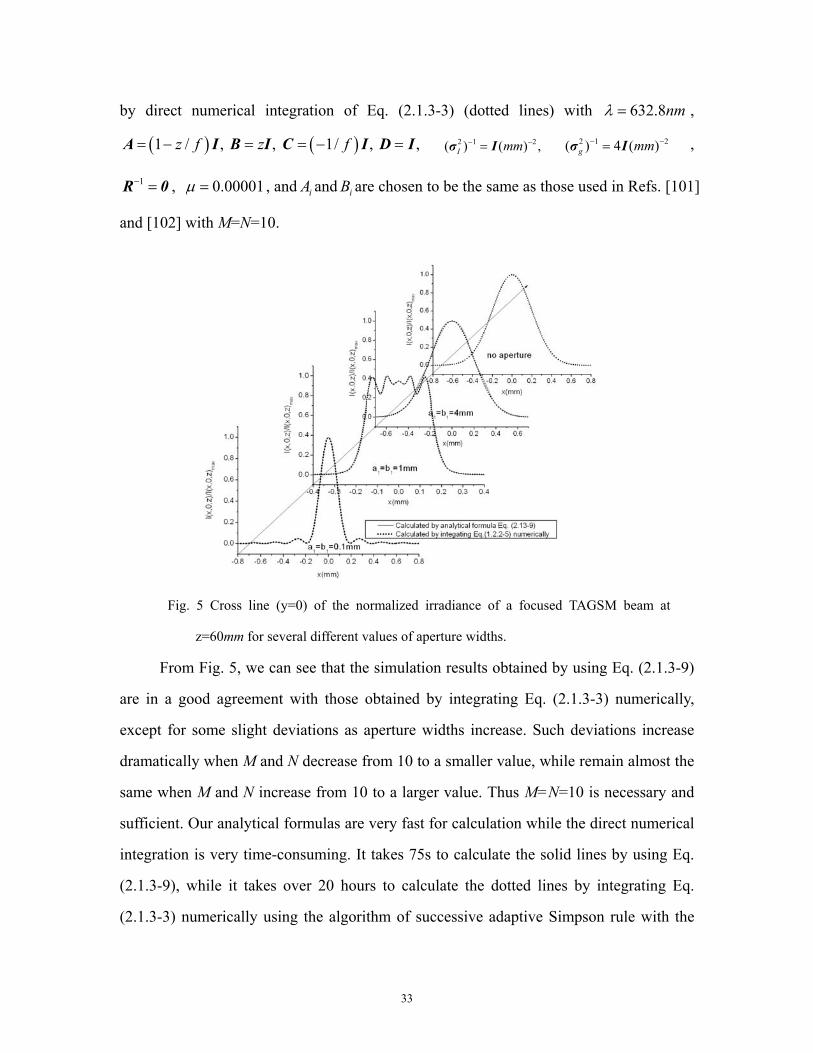
As numerical examples, we calculate and show in Fig. 5 the cross line (y=0) of the

normalized irradiance of a TAGSM beam at z=60mm after passing through a squarely

apertured ( 1 1a b= ) thin lens with focal length 50f mm= (located at z=0) for several

different values of aperture widths by using analytical formula (2.1.3-9) (solid lines) or

33

by direct numerical integration of Eq. (2.1.3-3) (dotted lines) with 632.8nmλ = ,

( ) ( )1 / , , 1/ , ,z f z f= − = = − =A I B I C I D I 2 1 2( ) ( ) ,I mm− −=σ I 2 1 2( ) 4 ( )g mm− −=σ I ,

1− =R 0 , 0.00001µ = , and iA and iB are chosen to be the same as those used in Refs. [101]

and [102] with M=N=10.

Fig. 5 Cross line (y=0) of the normalized irradiance of a focused TAGSM beam at

z=60mm for several different values of aperture widths.

From Fig. 5, we can see that the simulation results obtained by using Eq. (2.1.3-9)

are in a good agreement with those obtained by integrating Eq. (2.1.3-3) numerically,

except for some slight deviations as aperture widths increase. Such deviations increase

dramatically when M and N decrease from 10 to a smaller value, while remain almost the

same when M and N increase from 10 to a larger value. Thus M=N=10 is necessary and

sufficient. Our analytical formulas are very fast for calculation while the direct numerical

integration is very time-consuming. It takes 75s to calculate the solid lines by using Eq.

(2.1.3-9), while it takes over 20 hours to calculate the dotted lines by integrating Eq.

(2.1.3-3) numerically using the algorithm of successive adaptive Simpson rule with the

34

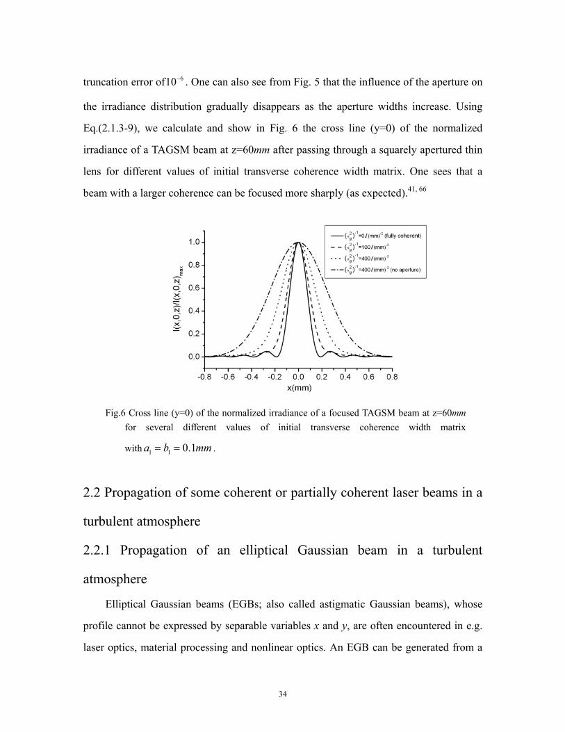
truncation error of 610− . One can also see from Fig. 5 that the influence of the aperture on

the irradiance distribution gradually disappears as the aperture widths increase. Using

Eq.(2.1.3-9), we calculate and show in Fig. 6 the cross line (y=0) of the normalized

irradiance of a TAGSM beam at z=60mm after passing through a squarely apertured thin

lens for different values of initial transverse coherence width matrix. One sees that a

beam with a larger coherence can be focused more sharply (as expected).41, 66

Fig.6 Cross line (y=0) of the normalized irradiance of a focused TAGSM beam at z=60mm

for several different values of initial transverse coherence width matrix

with 1 1 0.1a b mm= = .

2.2 Propagation of some coherent or partially coherent laser beams in a

turbulent atmosphere

2.2.1 Propagation of an elliptical Gaussian beam in a turbulent

atmosphere

Elliptical Gaussian beams (EGBs; also called astigmatic Gaussian beams), whose

profile cannot be expressed by separable variables x and y, are often encountered in e.g.

laser optics, material processing and nonlinear optics. An EGB can be generated from a

35

mode-locked laser beam, a frequency-double laser beam or a semiconductor laser beam

by e.g. focusing a Gaussian beam with a cylindrical lens. Since Arnaud and Kogelnik first

introduced an EGB in 1969,103 EGBs have been widely studied in both theoretical and

experimental aspects. Carter introduced the concept of a vectorial nonparaxial elliptical

Gaussian beam and derived the expression for the field components.104 The self-focusing

and rotating properties of an EGB in a nonlinear medium have also been analyzed.105

Alda et al. introduced a complex curvature tensor for the EGB and studied its propagation

through a complex optical system.15,106 Medhekar et al. studied the self-tapering of an

EGB in an elliptic-core nonlinear fiber.107 Freegarde et al. analyzed the second-harmonic

generation of type I with EGBs.108 Courtial et al. investigated an EGB with high orbital

angular momentum and its applications in rotating micron-sized particles.109 Mian et al.

analyzed the z-scan measurement with an EGB.110 More recently, Seshadri studied the

properties of an EGB in a uniaxial crystal.111 We have studied the propagation properties

of a decentered EGB in free space.112 The propagation properties of an EGB in a

turbulent atmosphere have not been studied before. In Paper IV, we study the average

intensity and spreading of an EGB in a turbulent atmosphere.

The propagation of a laser beam in a turbulent atmosphere can be treated by the

extended Huygens-Fresnel integral given by Eq. (1.1.3-3). After some rearrangement, we

can express Eq. (1.1.3-3) in the following tensor form

( )( )

( ) ( ) ( )2

* 1 1 11 21/ 22

, ,0 ,0 exp 224 det

exp , 2

T T

T

k ikI z E E

ik d

π

∞ ∞ ∞ ∞ − − −

−∞ −∞ −∞ −∞

= − − + × −

∫ ∫ ∫ ∫ρ r r r B r rB ρ ρ B ρΒ

r P r r (2.2.1-1)

where ( )1 2T T T=r r r , ( )T T T=ρ ρ ρ , and

,z

z

= −

I 0B

0 I 2

0

2 ,ikρ

− = −

I IP

I I (2.2.1-2)

and where I is a 2 2× unit matrix.

The electric field of a generalized EGB at z=0 can be expressed in the following

36

tensor form:

( ) 11 1 1 1,0 exp

2TikE − = −

r r Q r , (2.2.1-3)

where 11−Q is the complex curvature tensor. Then ( ) ( )*

1 2,0 ,0E Er r in Eq. (2.2.1-1) can

be expressed in the following tensor form

( ) ( ) ( )*2 2* 1 1 11 2 0 1 1 1 2 1 2 0 1,0 ,0 exp exp = exp

2 2 2T T Tik ik ikE E E E− − − = − −

r r r Q r r Q r r Q r

(2.2.1-4)

where( )

111

*1 11

−

−

−

= −

Q 0Q

0 Q.

Substituting Eq. (2.2.1-4) into Eq. (2.2.1-1), we obtain the following average

intensity of the EGB in the output plane after some vector integration

( ) ( ){ } ( )11/ 2 12 1 1

0 1 1, = det exp ,2

TikI z E−− −− − + + − + +

ρ I B Q P ρ Q P B ρ (2.2.1-5)

where I is a 4 4× unit matrix. Eq. (2.2.1-5) is convenient for use in analyzing the

propagation properties of the EGB in a turbulent atmosphere. In the absence of

turbulence ( 0ρ − > ∞ , i.e., 2 0nC = ), P =0 and consequently Eq. (2.2.1-5) reduces to the

well-established formula for an EGB propagating in free space. Eq. (2.2.1-5) is the main

result of Paper IV.

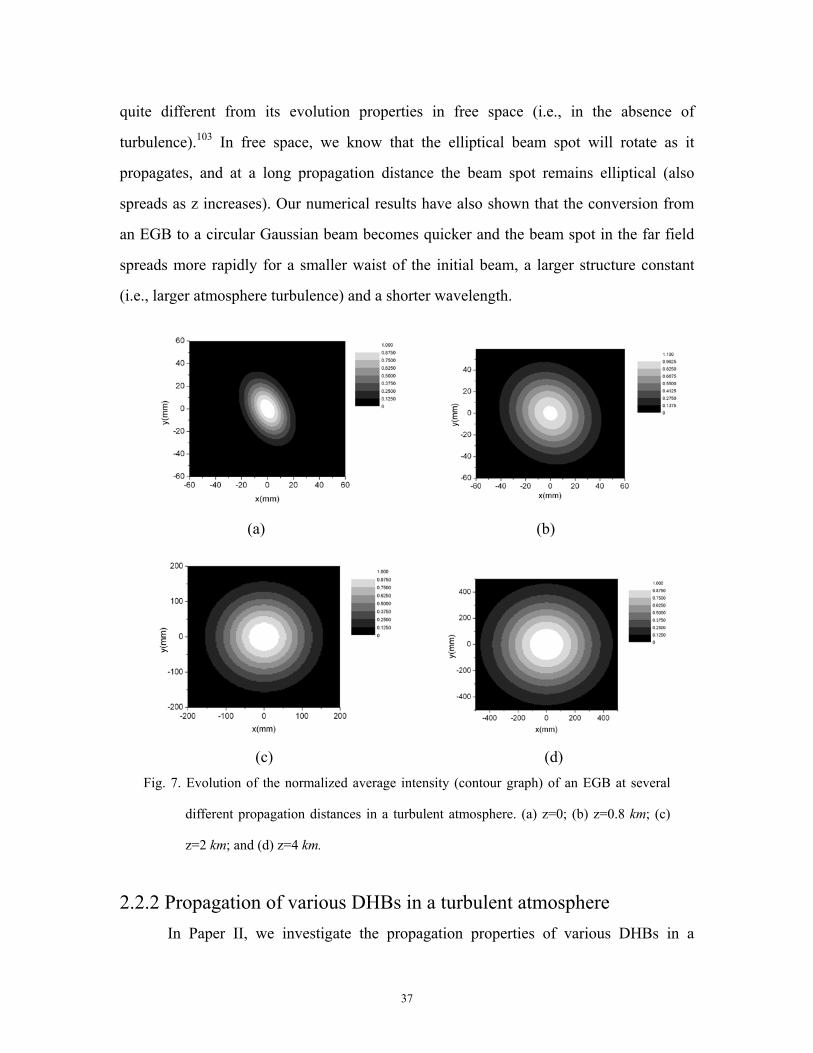
Using the formulae derived above, we illustrate numerically the intensity and

spreading properties of an EGB in a turbulent atmosphere. Fig. 7 (contour graph) shows

the evolution of the normalized average intensity of an EGB at several different

propagation distances in a turbulent atmosphere with 632.8nmλ = ,

0 020 , 30x yw mm w mm= = and 0 40xyw mm= , 2 13 2/310nC m− −= . From Fig. 7 one sees that

the ellipticity of the beam spot disappears gradually as z increases. The elliptical beam

spot gradually becomes a Gaussian (circular) beam spot (see Fig. 7(c)) after propagating

over a certain distance, and then spreads (see Fig. 7(d)) as z increases further. This is

37

quite different from its evolution properties in free space (i.e., in the absence of

turbulence).103 In free space, we know that the elliptical beam spot will rotate as it

propagates, and at a long propagation distance the beam spot remains elliptical (also

spreads as z increases). Our numerical results have also shown that the conversion from

an EGB to a circular Gaussian beam becomes quicker and the beam spot in the far field

spreads more rapidly for a smaller waist of the initial beam, a larger structure constant

(i.e., larger atmosphere turbulence) and a shorter wavelength.

(a) (b)

(c) (d)

Fig. 7. Evolution of the normalized average intensity (contour graph) of an EGB at several

different propagation distances in a turbulent atmosphere. (a) z=0; (b) z=0.8 km; (c)

z=2 km; and (d) z=4 km.

2.2.2 Propagation of various DHBs in a turbulent atmosphere

In Paper II, we investigate the propagation properties of various DHBs in a

38

turbulent atmosphere. Using Eq. (2.1.1-6), we can express ( ) ( )*1 2,0 ,0E Er r for a DHB

of circular or elliptical symmetry in the following tensor form

( ) ( ) ( )* 1 11 2 1 22

1 1

1 13 4

1,0 ,0 exp exp

2 2

exp exp , 2 2

n mN NT T

N N nm nmn m

T Tnm nm

N N ik ikE En mN

ik ik

+− −

= =

− −

− = − − − − − + −

∑∑r r r Q r r Q r

r Q r r Q r (2.2.2 1)−

where

( ) ( )

( ) ( )

1 11 11 1

* *1 21 11 1

1 11 11 1

* *3 41 11 1

, ,

, .

n n

nm nmm mp

np np

nm nmm mp

− −

− −

− −

− −

− −

− −

= = − − = = − −

Q 0 Q 0Q Q

0 Q 0 Q

Q 0 Q 0Q Q

0 Q 0 Q

(2.2.2-2)

Substituting Eq. (2.2.2-1) into Eq. (2.2.1-1), we obtain (after some vector integration) the

following expression for the average intensity of the DHB (of circular or elliptical

symmetry) propagating in a turbulent atmosphere

( ) ( ) [ ]

[ ] [ ]

[ ]

1/ 2 1 11 o12

1 1

1/ 2 1/ 21 1 1 12 o2 3 o3

1/4

1, = det exp

2

det exp det exp2 2

det

n mN NT

nmn m

T Tnm nm

N N ikI zn mN

ik ik

+− − −

= =

− −− − − −

−

− − − − − −

+

∑∑ρ S ρ Q ρ

S ρ Q ρ S ρ Q ρ

S 2 1 1o4exp , (2.2.2-3)

2T

nmik − − − ρ Q ρ

where

( )1i inm

−= + +S I B Q P , ( )111 1

oinm inm

−−− − = + + Q Q P B . (2.2.2-4)

Similarly, we can express ( ) ( )*1 2,0 ,0E Er r for a DHB of rectangular symmetry as

follows (using Eq. (2.1.1-7))

( ) ( ) ( )* 11 2 12 2

1 1 1 1

1 1 11 2 1 3 4

1,0 ,0 exp

2

exp exp exp , 2 2 2

h l n mH H N NT

HN HN hnlmh l n m

T T Thnlm hnlm hnlm

H H N N ikE Eh l n mN H

ik ik ik

+ + +−

= = = =

− − −

− = − − − − − + −

∑∑∑∑r r r Q r

r Q r r Q r r Q r (2.2.2-5)

39

where

( ) ( )

( ) ( )

1 11 11 1

* *1 21 11 1

1 11 11 1

* *3 41 11 1

, ,

, .

hn hn

hnlm hnlmlm lmp

hnp hnp

hnlm hnlmlm lmp

− −

− −

− −

− −

− −

− −

= = − − = = − −

Q 0 Q 0Q Q

0 Q 0 Q

Q 0 Q 0Q Q

0 Q 0 Q

(2.2.2-6)

Substituting Eq. (2.2.2-5) into Eq. (2.2.1-1), we obtain (after vector integration) the

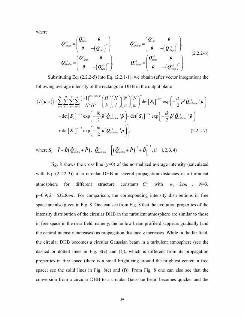
following average intensity of the rectangular DHB in the output plane

( ) ( ) [ ]

[ ] [ ]

1/ 2 1 11 o12 2

1 1 1 1

1/ 2 1/ 21 1 12 o2 3 o3

1, = det exp

2

det exp det exp2 2

h l n mH H N NT

hnlmh l n m

T Thnlm hnlm

H H N N ikI zh l n mN H

ik ik

+ + +− − −

= = = =

− −− − − −

− − − − − −

∑∑∑∑ρ S ρ Q ρ

S ρ Q ρ S ρ Q

[ ]

1

1/ 2 1 14 o4 det exp , (2.2.2-7)

2T

hnlmik− − −

+ −

ρ

S ρ Q ρ

where ( )1i ihnlm

−= + +S I B Q P , ( )111 1

o , ( 1, 2,3, 4)ihnlm ihnlm i−−− − = + + =

Q Q P B

Fig. 8 shows the cross line (y=0) of the normalized average intensity (calculated

with Eq. (2.2.2-3)) of a circular DHB at several propagation distances in a turbulent

atmosphere for different structure constants 2nC with 0 2w cm= , N=3,

p=0.9, 632.8nmλ = . For comparison, the corresponding intensity distributions in free

space are also given in Fig. 8. One can see from Fig. 8 that the evolution properties of the

intensity distribution of the circular DHB in the turbulent atmosphere are similar to those

in free space in the near field, namely, the hollow beam profile disappears gradually (and

the central intensity increases) as propagation distance z increases. While in the far field,

the circular DHB becomes a circular Gaussian beam in a turbulent atmosphere (see the

dashed or dotted lines in Fig. 8(e) and (f)), which is different from its propagation

properties in free space (there is a small bright ring around the brightest center in free

space; see the solid lines in Fig. 8(e) and (f)). From Fig. 8 one can also see that the

conversion from a circular DHB to a circular Gaussian beam becomes quicker and the

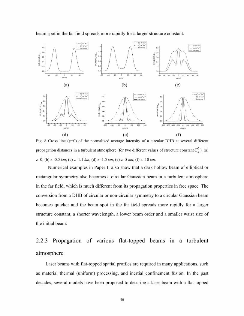
40

beam spot in the far field spreads more rapidly for a larger structure constant.

(a) (b) (c)

(d) (e) (f) Fig. 8 Cross line (y=0) of the normalized average intensity of a circular DHB at several different

propagation distances in a turbulent atmosphere (for two different values of structure constant 2nC ). (a)

z=0; (b) z=0.5 km; (c) z=1.1 km; (d) z=1.5 km; (e) z=5 km; (f) z=10 km.

Numerical examples in Paper II also show that a dark hollow beam of elliptical or

rectangular symmetry also becomes a circular Gaussian beam in a turbulent atmosphere

in the far field, which is much different from its propagation properties in free space. The

conversion from a DHB of circular or non-circular symmetry to a circular Gaussian beam

becomes quicker and the beam spot in the far field spreads more rapidly for a larger

structure constant, a shorter wavelength, a lower beam order and a smaller waist size of

the initial beam.

2.2.3 Propagation of various flat-topped beams in a turbulent

atmosphere

Laser beams with flat-topped spatial profiles are required in many applications, such

as material thermal (uniform) processing, and inertial confinement fusion. In the past

decades, several models have been proposed to describe a laser beam with a flat-topped

41

profile. The super-Gaussian beam is one of the models fulfilling the requirements.30 Gori

proposed another model called the flattened Gaussian beam, whose electric field can be

expanded as a finite sum of Laguerre-Gaussian modes or Hermite-Gaussian modes.31,113

More recently, Li proposed a new theoretical model to describe a flat-topped beam of

circular or non-circular symmetry by expressing its field as a finite sum of fundamental

Gaussian beams.32,33 We have introduced an elliptical flat-topped beam by expressing its

field as a sum of finite elliptical Gaussian beams in a tensor form.114 Coutts has generated

flat-topped beams with a copper vapour laser.115, 116 In practice, a laser beam generated by

an excimer laser is also flat-topped.117,118 Propagation of various flat-topped beam

through a paraxial optical system or free space has been studied extensively in the last

decade. In Paper V, we investigate the propagation of various flat-topped beams in a

turbulent atmosphere.

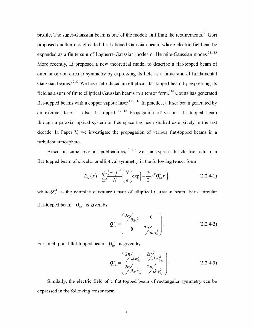
Based on some previous publications,32, 114 we can express the electric field of a

flat-topped beam of circular or elliptical symmetry in the following tensor form

( ) ( ) 11

11

1exp

2

nNT

N nn

N ikEnN

−−

=

− = −

∑r r Q r , (2.2.4-1)

where 11n−Q is the complex curvature tensor of elliptical Gaussian beam. For a circular

flat-topped beam, 11n−Q is given by

201

1

20

2 0

20n

nikw

nikw

−

=

Q . (2.2.4-2)

For an elliptical flat-topped beam, 11n−Q is given by

2 20 01

1

2 20 0

2 2

2 2x xy

n

xy y

n nikw ikw

n nikw ikw

−

=

Q . (2.2.4-3)

Similarly, the electric field of a flat-topped beam of rectangular symmetry can be

expressed in the following tensor form

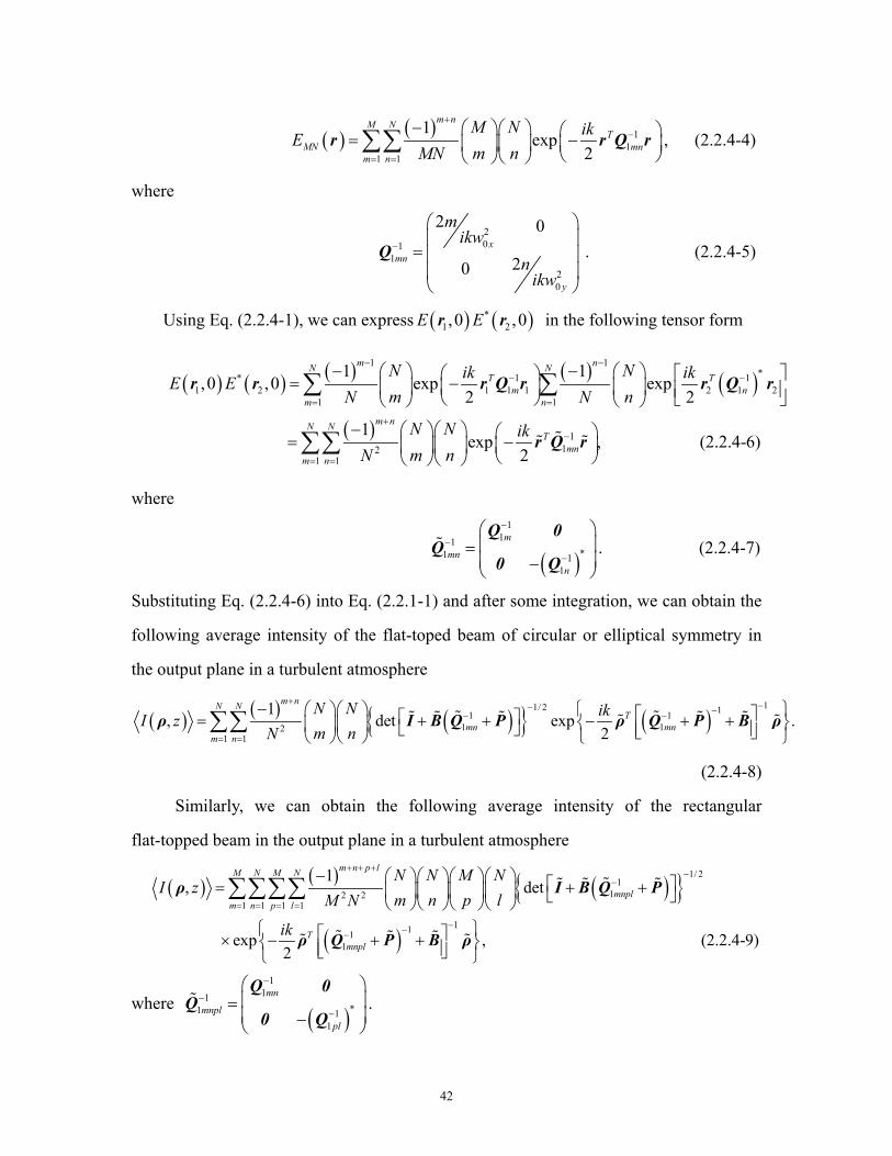
42

( ) ( ) 11

1 1

1exp

2

m nM NT

MN mnm n

M N ikEm nMN

+−

= =

− = −

∑∑r r Q r , (2.2.4-4)

where

201

120

2 0

20x

mn

y

mikw

nikw

−

=

Q . (2.2.4-5)

Using Eq. (2.2.4-1), we can express ( ) ( )*1 2,0 ,0E Er r in the following tensor form

( ) ( ) ( ) ( ) ( )

( )

1 1** 1 1

1 2 1 1 1 2 1 21 1

112

1 1

1 1,0 ,0 exp exp

2 2

1 exp ,

2

m nN NT T

m nm n

m nN NT

mnm n

N Nik ikE Em nN N

N N ikm nN

− −− −

= =

+−

= =

− − = −

− = −

∑ ∑

∑∑

r r r Q r r Q r

r Q r (2.2.4-6)

where

( )

111

*1 11

m

mnn

−

−

−

= −

Q 0Q

0 Q. (2.2.4-7)

Substituting Eq. (2.2.4-6) into Eq. (2.2.1-1) and after some integration, we can obtain the

following average intensity of the flat-toped beam of circular or elliptical symmetry in

the output plane in a turbulent atmosphere

( ) ( ) ( ){ } ( )11/ 2 11 1

1 121 1

1, det exp .

2

m nN NT

mn mnm n

N N ikI zm nN

+ −− −− −

= =

− = + + − + + ∑∑ρ I B Q P ρ Q P B ρ

(2.2.4-8)

Similarly, we can obtain the following average intensity of the rectangular

flat-topped beam in the output plane in a turbulent atmosphere

( ) ( ) ( ){ }( )

1/ 21

12 21 1 1 1

1111

1, det

exp , 2

m n p lM N M N

mnplm n p l

Tmnpl

N N M NI z

m n p lM N

ik

+ + +−

−

= = = =

−−−

− = + + × − + +

∑∑∑∑ρ I B Q P

ρ Q P B ρ (2.2.4-9)

where ( )

111

*1 11

mn

mnplpl

−

−

−

= −

Q 0Q

0 Q.

43

Eqs. (2.2.4-8) and (2.2.4-9) provide a convenient way for studying the

propagation properties of various flat-topped beams in a turbulent atmosphere. Numerical

results in paper V show that a flat-topped beam of circular or non-circular symmetry also

becomes a circular Gaussian beam in a turbulent atmosphere in the far field. The

conversion from a flat-topped beam of circular or non-circular symmetry to a circular

Gaussian beam becomes quicker and the beam spot in the far field spreads more rapidly

for a larger structure constant, a shorter wavelength, a lower beam order and a smaller

waist size of the initial beam.

2.2.4 Propagation of a partially coherent TAGSM beam in a turbulent

atmosphere

Propagation of partially coherent beams in a turbulent atmosphere has been

extensively studied in the past decades.20-23 More recently, Ricklin et al theoretically

analyzed the application of partially coherent Gaussian Schell-model (GSM) beams in

free-space communication, and found that applications of partially coherent beams can

result in a significant reduction in the bit error rate of an optical communication link as

compared with a coherent beam.24 The partially coherent beams considered in the

relevant literature are stigmatic and their profiles can be expressed by separable variables

x and y. Propagation of an astigmatic partially coherent beam in a turbulent atmosphere

has not been studied before. In Paper VI, we investigate the propagation properties of a

TAGSM beam (general astigmatic partially coherent beam) in a turbulent atmosphere.

The propagation formula for the cross-spectral density of a partially coherent beam

through a turbulent atmosphere is given by Eq. (1.2.2-7), which can be expressed in the

following tensor form after some rearrangement,

44

( )( )

21 1 1

2 11/ 22 ( , ) ( , ) exp 2

24 det

exp , 2

T T

T

k ikW z W z

ik d

π

∞ ∞ ∞ ∞ − − −

−∞ −∞ −∞ −∞

= − − + × −

∫ ∫ ∫ ∫ρ r r B r rB ρ ρ B ρΒ

r P r r (2.2.4-1)

where ( )1 2T T T=r r r , ( )1 2

T T T=ρ ρ ρ , B and P are given by Eq. (2.2.1-2)

Substituting Eq. (2.1.3-1) into Eq. (2.2.5-1), we obtain the following

cross-spectral density of the twisted AGSM in the output plane after some vector

integration,

( ) 1/ 21 12 1 2 ( , ; )= det exp ,

2TikW z w

−− − + + −

ρ I BM BP ρ M ρ (2.2.4-2)

where 12−M denotes the partially coherent complex curvature tensor in the output plane,

and is related to 11−M by the following formula

( )111 1

2 1

−−− − = + + M M P B . (2.2.4-3)

If we set 2 20I Iσ=σ I , 2 2

0g gσ=σ I , 1 0,− =R 0µ = , Eq. (2.2.4-2) reduces to the

propagation formula for a partially coherent isotropic GSM in the turbulent atmosphere.

If we set 2 20I Iσ=σ I , 2 0g =σ I , 1 0,− =R 0µ = , Eq. (2.2.4-2) reduces to the propagation

formula for a coherent Gaussian beam in the turbulent atmosphere.

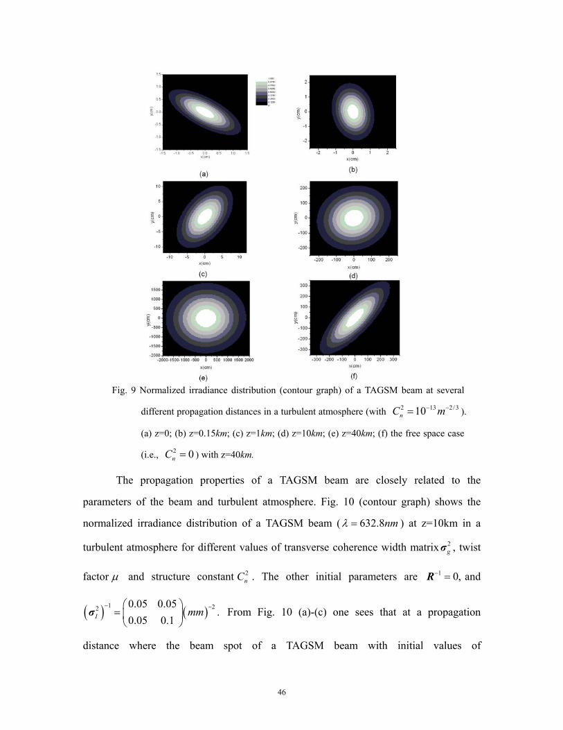
Fig. 9(a)-(e) (contour graph) show the normalized irradiance distribution of a

TAGSM beam ( 632.8nmλ = ) at several different propagation distances in a turbulent

atmosphere. The initial parameters at z=0 are 1 0,− =R ( ) 10.000005 mmµ −= ,

2 13 2/310nC m− −= , ( ) ( )1 22 0.05 0.05,

0.05 0.1I mm− − =

σ ( ) ( )1 22 0.05g mm− −=σ I . For comparison,

the far field irradiance distribution of a TAGSM beam in free space is also shown in Fig.

45

9(f). From Fig. 9(a)-(c) one sees that in the near field the propagation of a TAGSM beam

is similar to that in free space, for example, the elliptical beam spot TAGSM rotates

clockwise (it will rotates anti-clockwise if 0µ < ) gradually as z increases.16-22 While in

the far field (after stop rotating) the elliptical beam gradually becomes a circular beam

spot (see Fig. 9 (d)-(e)) and then spreads as z increases further, which means that the

TAGSM beam eventually becomes a partially coherent stigmatic (isotropic) beam under

the influence of the atmospheric turbulence. These interesting propagation properties are

quite different from those in free space. In free space, the beam spot of a TAGSM beam

remains elliptical in the far field and spreads as z increases (cf. Fig. 9 (a) and (f)). From

Eq. (2.2.4-3), we can find that 10−M in the output plane is determined by 1

s−M (source’s

complex curvature tensor), P (atmospheric turbulence) and B . In the near field, 1s−M

is much larger than P , the influence of the turbulence is small, and thus the propagation

properties (mainly determined by 1s−M and B ) are similar to those in free space. As z

increases further, P increases gradually and becomes eventually larger than 1s−M (then

the propagation properties are mainly determined by P and B ), and this leads to the

above interesting phenomena of the TAGSM beam propagating in a turbulent

atmosphere.

46

Fig. 9 Normalized irradiance distribution (contour graph) of a TAGSM beam at several

different propagation distances in a turbulent atmosphere (with 2 13 2/310nC m− −= ).

(a) z=0; (b) z=0.15km; (c) z=1km; (d) z=10km; (e) z=40km; (f) the free space case

(i.e., 2 0nC = ) with z=40km.

The propagation properties of a TAGSM beam are closely related to the

parameters of the beam and turbulent atmosphere. Fig. 10 (contour graph) shows the

normalized irradiance distribution of a TAGSM beam ( 632.8nmλ = ) at z=10km in a

turbulent atmosphere for different values of transverse coherence width matrix 2gσ , twist

factor µ and structure constant 2nC . The other initial parameters are 1 0,− =R and

( ) ( )1 22 0.05 0.05.

0.05 0.1I mm− − =

σ From Fig. 10 (a)-(c) one sees that at a propagation

distance where the beam spot of a TAGSM beam with initial values of

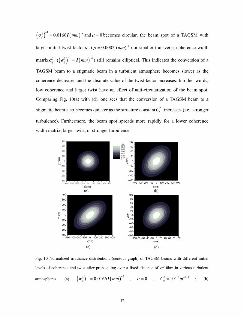
47

( ) ( )1 22 0.0166g mm− −=σ I and 0µ = becomes circular, the beam spot of a TAGSM with

larger initial twist factorµ ( 10.0002 ( )mmµ −= ) or smaller transverse coherence width

matrix 2gσ ( ( ) ( )1 22

g mm− −=σ I ) still remains elliptical. This indicates the conversion of a

TAGSM beam to a stigmatic beam in a turbulent atmosphere becomes slower as the

coherence decreases and the absolute value of the twist factor increases. In other words,

low coherence and larger twist have an effect of anti-circularization of the beam spot.

Comparing Fig. 10(a) with (d), one sees that the conversion of a TAGSM beam to a

stigmatic beam also becomes quicker as the structure constant 2nC increases (i.e., stronger

turbulence). Furthermore, the beam spot spreads more rapidly for a lower coherence

width matrix, larger twist, or stronger turbulence.

Fig. 10 Normalized irradiance distributions (contour graph) of TAGSM beams with different initial

levels of coherence and twist after propagating over a fixed distance of z=10km in various turbulent

atmospheres. (a) ( ) ( )1 22 0.0166g mm− −=σ I , 0µ = , 2 13 2/310nC m− −= ; (b)

48

( ) ( )1 22 0.0166g mm− −=σ I , 10.0002 ( )mmµ −= , 2 13 2/310nC m− −= ; (c) ( ) ( )1 22

g mm− −=σ I ,

0µ = , 2 13 2/310nC m− −= ; (d) ( ) ( )1 22 0.0166g mm− −=σ I , 0µ = , 2 14 2/310nC m− −=

2.3 Coincidence fractional Fourier transform

2.3.1. Coincidence fractional Fourier transform with incoherent or

partially coherent light Coincidence Fourier optics including coincidence imaging and diffraction (also

called ghost imaging and diffraction) has been extensively investigated due to its great

potential applications in metrology, lithography and holography, etc.46-48,119-125 The

coincidence Fourier optics is a method to obtain the image or Fourier transform

(diffraction) of an object by measuring the coincidence counting rate (i.e., the fourth

order correlation) of two detected signals going through two different light paths. In

paper VII, we introduce the coincidence fractional Fourier transform (FRT) with

incoherent or partially coherent light, and design the optical system to implement the

coincidence FRT.

Fig.11 shows the optical system for implementing the coincidence FRT with

incoherent light. The incoherent light is split by a beam splitter. Then the two emerging

beams propagate through either path one or path two to detector D1 or D2.. D1 is a

single-photon detector and D2 is an array of pixel detectors. In path one, between the

beam splitter and D1 there is an object with transmision function ( )vH , and between the

object and D1 there is a thin lens with focal length 1f . Both distances from the object to

the lens and the object to D1 are 1f . In Path two, there is a thin lens with focal length f

between the beam splitter and D2, and the distances from the light source to the lens and

the lens to D2 are 21 and ll , respectively. The coincident counting rate of the two detected

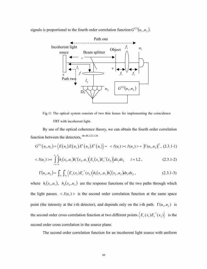
49

signals is proportional to the fourth order correlation function ( ) ( )212 ,uuG .

Fig.11 The optical system consists of two thin lenses for implementing the coincidence

FRT with incoherent light.

By use of the optical coherence theory, we can obtain the fourth order correlation

function between the detectors, 46-48,122-126

( ) ( ) ( ) ( ) ( ) 2(2)1 2 1 2 2 1 1 2 1 2, ( ) ( ) ( , ) , (2.3.1-1)G u u E u E u E u E u I u I u u u∗ ∗= = < >< > + Γ

( ) ( ) ( ) ( ) 2,1 ,,)( 212121 =>=< ∫ ∫∞

∞−

∞

∞−

∗∗ idxdxxExEuxhuxhuI ssiiiii , (2.3.1-2)

( ) ( ) ( )∫ ∫∞

∞−

∞

∞−=Γ 2122

*21112

*121 ,,)()(, dxdxuxhuxhxExEuu ss , (2.3.1-3)

where ( )111 ,uxh , ( )222 ,uxh are the response functions of the two paths through which

the light passes. >< )( iuI is the second order correlation function at the same space

point (the intensity at the i-th detector), and depends only on the i-th path. ),( 21 uuΓ is

the second order cross correlation function at two different points. )()( 2*

1 xExE ss is the

second order cross correlation in the source plane.

The second order correlation function for an incoherent light source with uniform

x

Object

( ) ( )212 ,uuG

z

Incoherent light souce

D2

Beam splitter

1l

1u

2u

v 1f 1f

1f

2l

f

Path one

Path two

50

intensity distribution 0I can be expressed as:

( ) ( ) ( )1 2 0 1 2s sE x E x I x xδ∗ = − . (2.3.1-4)

Substituting Eq. (2.3.1-4) and expressions for ( )1 1 1,h x u and ( )2 2 2,h x u into Eqs.

(2.3.1-1)-(2.3.1-3), we obtain

( )1 20 ( )I u I u< = >< >= ∞ , (2.3.1-5)

( ) ( )2 201 2 1 1 2 1 2 12

1

2( 0, ) exp , tan sinsin e ee

I i iu u H v v u v u dvf ff fπ π

λ φ λ φλ φ

∞

−∞

Γ = = + −

∫

(2.3.1-6)

where ( )1H v is the transmission function of the object. Here we have assumed that

1 2tan / 2 , tan / 2, / sin ,e e el f z l f f fφ φ φ= + = = (2.3.1-7)

where ef is called the “standard focal length”,74 φ is defined by 2/πφ p= , and p is the

desired fractional order of the FRT. Eq. (2.3.1-6) gives the FRT expression of the object.

The parameters for the optical system can be determined from Eq. (2.3.1-7) for the

desired ef and p. The visibility of the coincidence FRT pattern is defined as

( ) ( )2 (2)1 2 1 2 maxmax

0, / 0,V u u G u u= Γ = = . Since both ( )1 20 ( )I u I u< = >< > and

1 2( 0, )u uΓ = contribute to the coincident counting rate, the visibility of the FRT pattern

of an object is practically zero for an incoherent light since ( )1 20 ( )I u I u< = >< >= ∞ ..

To obtain an observable coincidence FRT, we need to consider how to increase the

visibility. This can be achieved by replacing the incoherent light with a partially coherent

light.

Here we consider a typical partially coherent light source, namely, a partially

coherent Gaussian Schell-model (GSM) source. The second order correlation function in

the GSM source plane has the following form:54-57

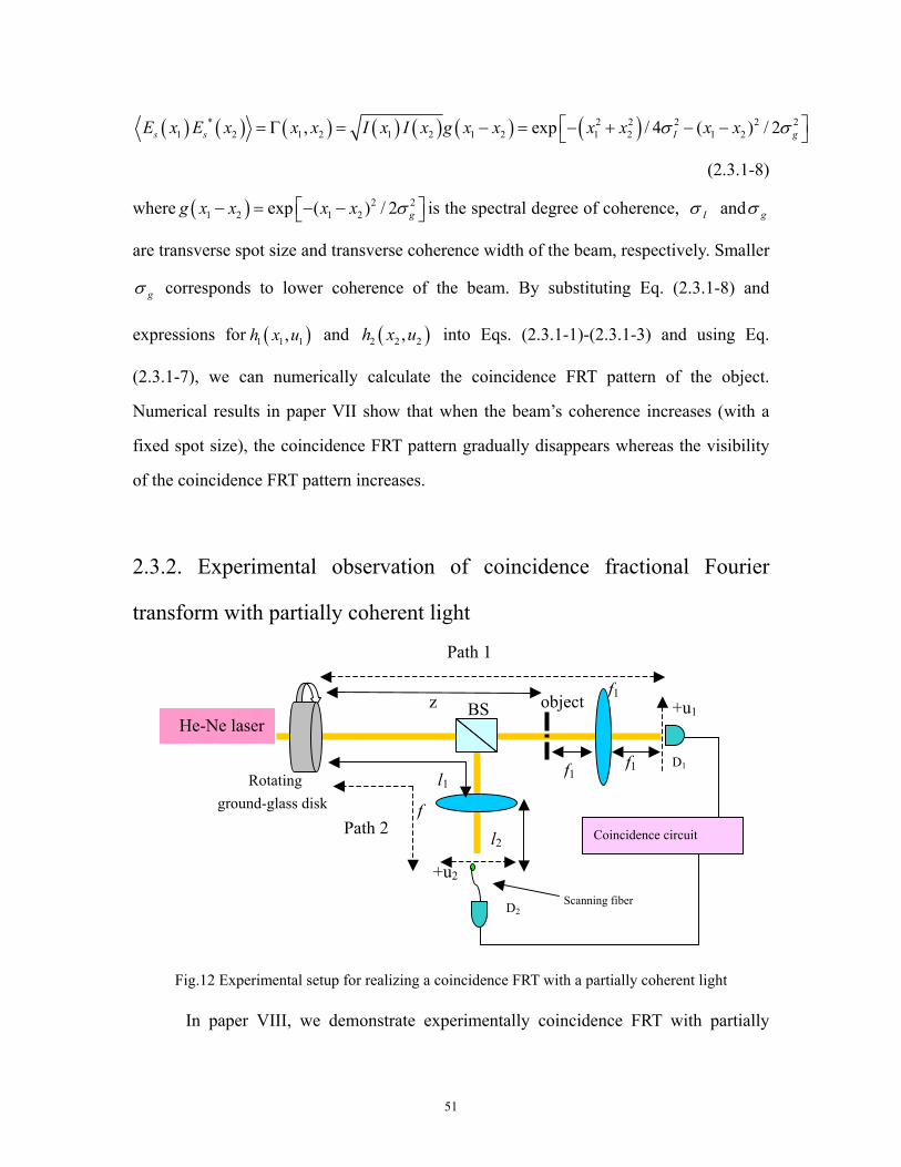
51

( ) ( ) ( ) ( ) ( ) ( ) ( )* 2 2 2 2 21 2 1 2 1 2 1 2 1 2 1 2, exp / 4 ( ) / 2s s I gE x E x x x I x I x g x x x x x xσ σ = Γ = − = − + − −

(2.3.1-8)

where ( ) 2 21 2 1 2exp ( ) / 2 gg x x x x σ − = − − is the spectral degree of coherence, Iσ and gσ

are transverse spot size and transverse coherence width of the beam, respectively. Smaller

gσ corresponds to lower coherence of the beam. By substituting Eq. (2.3.1-8) and

expressions for ( )1 1 1,h x u and ( )2 2 2,h x u into Eqs. (2.3.1-1)-(2.3.1-3) and using Eq.

(2.3.1-7), we can numerically calculate the coincidence FRT pattern of the object.

Numerical results in paper VII show that when the beam’s coherence increases (with a

fixed spot size), the coincidence FRT pattern gradually disappears whereas the visibility

of the coincidence FRT pattern increases.

2.3.2. Experimental observation of coincidence fractional Fourier

transform with partially coherent light

Fig.12 Experimental setup for realizing a coincidence FRT with a partially coherent light

In paper VIII, we demonstrate experimentally coincidence FRT with partially

z

f

+u1 BS object f1

f1 f1 Rotating ground-glass disk

D1

D2

l1

l2

He-Ne laser

+u2

Path 1

Path 2

Scanning fiber

Coincidence circuit

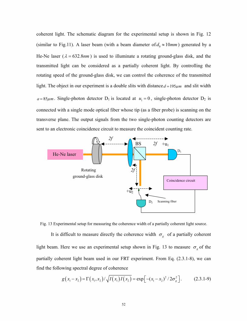
52

coherent light. The schematic diagram for the experimental setup is shown in Fig. 12

(similar to Fig.11). A laser beam (with a beam diameter of 0 10d mm≈ ) generated by a

He-Ne laser ( 632.8nmλ = ) is used to illuminate a rotating ground-glass disk, and the

transmitted light can be considered as a partially coherent light. By controlling the

rotating speed of the ground-glass disk, we can control the coherence of the transmitted

light. The object in our experiment is a double slits with distance 195d mµ= and slit width

85a mµ= . Single-photon detector D1 is located at 1 0u = , single-photon detector D2 is

connected with a single mode optical fiber whose tip (as a fiber probe) is scanning on the

transverse plane. The output signals from the two single-photon counting detectors are

sent to an electronic coincidence circuit to measure the coincident counting rate.

Fig. 13 Experimental setup for measuring the coherence width of a partially coherent light source.

It is difficult to measure directly the coherence width gσ of a partially coherent

light beam. Here we use an experimental setup shown in Fig. 13 to measure gσ of the

partially coherent light beam used in our FRT experiment. From Eq. (2.3.1-8), we can

find the following spectral degree of coherence

( ) ( ) ( ) ( ) 2 21 2 1 2 1 2 1 2, / exp ( ) / 2 gg x x x x I x I x x x σ − = Γ = − − . (2.3.1-9)

2f

+u1 BS 2f

Rotating ground-glass disk

D1

D2

+u2

Scanning fiber

He-Ne laser

2f

Coincidence circuit

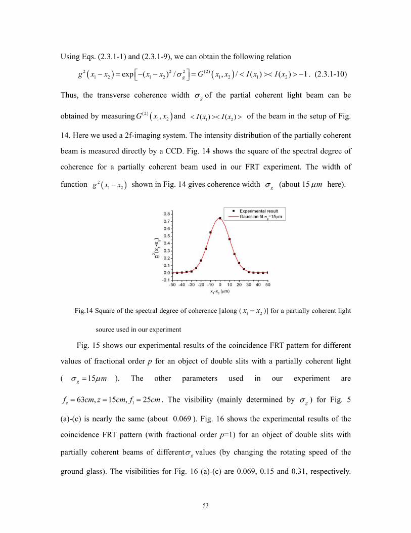
53

Using Eqs. (2.3.1-1) and (2.3.1-9), we can obtain the following relation

( ) ( )2 2 2 (2)1 2 1 2 1 2 1 2exp ( ) / , / ( ) ( ) 1gg x x x x G x x I x I xσ − = − − = < >< > − . (2.3.1-10)

Thus, the transverse coherence width gσ of the partial coherent light beam can be

obtained by measuring ( )(2)1 2,G x x and 1 2( ) ( )I x I x< >< > of the beam in the setup of Fig.

14. Here we used a 2f-imaging system. The intensity distribution of the partially coherent

beam is measured directly by a CCD. Fig. 14 shows the square of the spectral degree of

coherence for a partially coherent beam used in our FRT experiment. The width of

function ( )21 2g x x− shown in Fig. 14 gives coherence width gσ (about 15 mµ here).

Fig.14 Square of the spectral degree of coherence [along ( 1 2x x− )] for a partially coherent light

source used in our experiment

Fig. 15 shows our experimental results of the coincidence FRT pattern for different

values of fractional order p for an object of double slits with a partially coherent light

( 15g mσ µ= ). The other parameters used in our experiment are

163 , 15 , 25ef cm z cm f cm= = = . The visibility (mainly determined by gσ ) for Fig. 5

(a)-(c) is nearly the same (about 0.069 ). Fig. 16 shows the experimental results of the

coincidence FRT pattern (with fractional order p=1) for an object of double slits with

partially coherent beams of different gσ values (by changing the rotating speed of the

ground glass). The visibilities for Fig. 16 (a)-(c) are 0.069, 0.15 and 0.31, respectively.

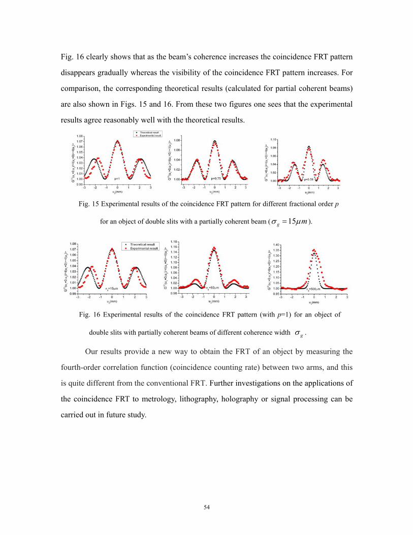
54

Fig. 16 clearly shows that as the beam’s coherence increases the coincidence FRT pattern

disappears gradually whereas the visibility of the coincidence FRT pattern increases. For

comparison, the corresponding theoretical results (calculated for partial coherent beams)

are also shown in Figs. 15 and 16. From these two figures one sees that the experimental

results agree reasonably well with the theoretical results.

Fig. 15 Experimental results of the coincidence FRT pattern for different fractional order p

for an object of double slits with a partially coherent beam ( 15g mσ µ= ).

Fig. 16 Experimental results of the coincidence FRT pattern (with p=1) for an object of

double slits with partially coherent beams of different coherence width gσ .

Our results provide a new way to obtain the FRT of an object by measuring the

fourth-order correlation function (coincidence counting rate) between two arms, and this

is quite different from the conventional FRT. Further investigations on the applications of

the coincidence FRT to metrology, lithography, holography or signal processing can be

carried out in future study.

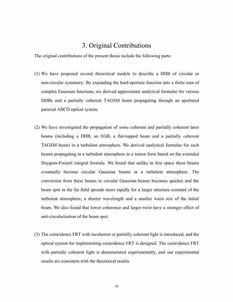
55

3. Original Contributions The original contributions of the present thesis include the following parts:

(1) We have proposed several theoretical models to describe a DHB of circular or

non-circular symmetry. By expanding the hard-aperture function into a finite sum of

complex Gaussian functions, we derived approximate analytical formulae for various

DHBs and a partially coherent TAGSM beam propagating through an apertured

paraxial ABCD optical system.

(2) We have investigated the propagation of some coherent and partially coherent laser

beams (including a DHB, an EGB, a flat-topped beam and a partially coherent

TAGSM beam) in a turbulent atmosphere. We derived analytical formulas for such

beams propagating in a turbulent atmosphere in a tensor form based on the extended

Huygens-Fresnel integral formula. We found that unlike in free space these beams

eventually become circular Gaussian beams in a turbulent atmosphere. The

conversion from these beams to circular Gaussian beams becomes quicker and the

beam spot in the far field spreads more rapidly for a larger structure constant of the

turbulent atmosphere, a shorter wavelength and a smaller waist size of the initial

beam. We also found that lower coherence and larger twist have a stronger effect of

anti-circularization of the beam spot.

(3) The coincidence FRT with incoherent or partially coherent light is introduced, and the

optical system for implementing coincidence FRT is designed. The coincidence FRT

with partially coherent light is demonstrated experimentally, and our experimental

results are consistent with the theoretical results.

56

4. Conclusion and Future Work In the present thesis, we have investigated the propagation of some coherent and partially

coherent laser beams. First we have proposed several theoretical models to describe a

DHB beam of circular or non-circular symmetry, and have derived approximate

analytical propagation formulas for a DHB or a TAGSM beam through an apertured

optical system. Our formulas avoid time-consuming numerical integration and provide a

convenient and effective way for studying the propagation of these beams through an

apertured paraxial ABCD optical system. Secondly, we have derived analytical formulas

for a DHB, an EGB, a flat-topped beam and a partially coherent TAGSM beam

propagating in a turbulent atmosphere based on the extended Huygens-Fresnel integral

formula. Our formulas provide a convenient way for treating the propagation of various

laser beams in a turbulent atmosphere. We have found some interesting propagation

properties of these beams in a turbulent atmosphere, which are quite different from their

propagation properties in free space. Finally, we have introduced the coincidence FRT

with an incoherent or partially coherent beam, and designed the optical system for its

implementation. We have demonstrated experimentally the coincidence FRT with a

partially coherent beam. The coincidence FRT provides a novel way to obtain the FRT

pattern of an object, and has great potential applications in metrology, lithography,

holography and signal processing, etc.

The following research can be carried out in future:

1. All the works in the present thesis were carried out under the paraxial condition. The

paraxial condition can be relaxed for a more general case. Some non-paraxial

propagation of these complicated laser beams and their applications in free-space

optical communication can be studied.

57

2. Astigmatic Gaussian beams can possess very high orbital momentum which is very

useful in atomic physics. It is anticipated that complicated astigmatic beams such

elliptical DHBs, elliptical flat-topped beams and TAGSM beams may also possess

high orbital momentum. Thus, further investigations on the orbital momentum of

these astigmatic laser beam and their interactions with atoms or micro-particles can

be done.

3. Recently, atom laser beams attract more and more attention. ABCD law for treating

the propagation of an atom laser beam has been derived. The beam quality for an

atom laser beam has also been defined. While the coherence properties of an

atom-laser beam has not been considered in the literature. Investigations of a partially

coherent atom-laser beam and its propagation are interesting.

4. Applications of coincidence FRT in metrology, lithography, holography and signal

processing need further investigation. Since it is very difficult to fabricate optical

components (such as lenses) working in x- orγ -ray regime, it would be interesting

and of practical significance to design some novel lensless optical system to

implement the coincidence FRT.

58

References 1. A. E. Siegman, Laser, University Science Books, Mill Valley, CA, 1986.

2. A. E. Siegman, Laser beams and resonators: Beyond the 1960s. IEEE. J. Special Topics in

Quantum Electron. XX, 100-110 (1999)

3. L. Allen, M. W. Beijersbergen, R. J. C. Spreeuw, and J. P. Woerdman. Orbital angular momentum

of light and the transformation of Laguerre-Gaussian laser modes. Phys. Rev. A, 45, 8185-8189

(1992)

4. A. E. Siegman. Hermite–gaussian functions of complex argumentas optical-beam eigenfunctions.

J. Opt. Soc. Am., 63, 1093–1094 (1973).

5. F. Gori, G. Guattari and C. Padovani. Bessel-Gaussian beams. Optics Comm. 64 491-495 (1987).

6. L. W. Casperson and A. A. Tovar. Hermite–sinusoidal-Gaussian beams in complex optical

systems. J. Opt. Soc. Am. A 15, 954–961 (1998).

7. M. J. Bastianns. The Wigner distribution function applied to optical signals and systems. Opt.

Commun. 25, 26-30 (1978).

8. R. Simon and G. S. Agarwal. Wigner representation of Laguerre–Gaussian beams. Opt. Lett. 25,

1313–1315 (2000).

9. T. J. Bruegge, M. P. Rimmer, and J. D. Targove. Software for free-space beam propagation. in

Optical Design and Analysis Software, R.C. Juergens, Eds, Proc. SPIE 3780, 14-22 (1999)

10. M. M. Popov. A new method of computation of wave fields using Gaussian beams. Wave Motion

4, 85-97 (1982)

11. M. A. Alonso and G. W. Forbes. Stable aggregates of flexible elements give a stronger link

between rays and waves. Opt. Exp. 10, 728-739 (2002)

12. S. Wang, L. Ronchi, Principles and Design of optical Array. In: E. Wolf editor. Progress in Optics,

vol.25, Amsterdan: Elsevier Science BV, 1988. p.279

13. J. A. Arnaud, Hamiltonian theory of beam mode propagation, in Progress in Optics, Vol XI, E.

Wolf, ed., North-Holland, Amsterdam, 1973, pp. 247-304.

59

14. J. A. Arnaud. Nonorthogonal optical waveguides and resonators. Bell Syst. Tech. J. 49,

2311-2348 (1970).

15. Q. Lin, S. Wang, J. Alda, and E. Bernabeu. Transformation of non-symmetric gaussian beam into

symmetric one by means of tensor ABCD law. Optik 85, 67-72 (1990).

16. C. C. Davis, I. I. Smolyaninov, and S. D. Milner. Flexible optical wireless link and networks.

IEEE Commun. Mag. 41, 51-57 (2003).

17. H. Izadpanah, T. Elbatt, V. Kukshya, F. Dolezal, and B. K. Ryu. High-availability free space

optical and RF hybrid wireless networks. IEEE Wireless Commun. 10, 45-55 (2003).

18. Z. I. Feizulin and Y. A. Kravtsov. Broadening of a laser beam in a turbulent medium. Radiophys.

Quantum Electron. 10, 33-35 (1967).

19. C. Y. Young, Y. V. Gilchrest, and B. R. Macon. Turbulence-induced beam spreading of

higher-order mode optical waves. Opt. Eng. 41, 1097-1103 (2002).

20. J. C. Leader. Atmospheric propagation of partially coherent radiation. J. Opt. Soc. Am. 68,

175-185 (1978).

21. S. C. H. Wang and M. A. Plonus. Optical beam propagation for a partially coherent source in the

turbulent atmosphere. J. Opt. Soc. Am. 69, 1297-1304 (1979).

22. T. Shirai, A. Dogariu, and E. Wolf. Mode analysis of spreading of partially coherent beams

propagating through atmospheric turbulence. J. Opt. Soc. Am. A 20, 1094-1102 (2003).

23. T. Shirai, A. Dogariu, and E. Wolf. Directionality of Gaussian Schell-model beams propagating

in atmospheric turbulence. Opt. Lett. 28, 610-612 (2003)

24. J. C. Ricklin and F. M. Davidson. Atmospheric turbulence effects on a partially coherent

Gaussian beam: implications for free-space laser communication. J. Opt. Soc. Am. A 19,

1794–1802 (2002).

25. H. T. Eyyuboğlu and Y. Baykal. Reciprocity of cos-Gaussian and cosh-Gaussian laser beams in

turbulent atmosphere. Opt. Express 12, 4659-4674 (2004).

26. H. T. Eyyuboğlu and Y. Baykal. Average intensity and spreading of cosh-Gaussian beams in the

turbulent atmosphere. Appl. Opt. 44, 976-983 (2005).

60

27. Y. Baykal. Correlation and structure functions of Hermite-sinusoidal-Gaussian laser beams in a

turbulent atmosphere. J. Opt. Soc. Am. A 21, 1290-1299 (2004).

28. H. T. Eyyuboğlu. Hermite-cosine-Gaussian laser beam and its propagation characteristics in

turbulent atmosphere. J. Opt. Soc. Am. A 22, 1527-1535 (2005).

29. H. T. Eyyuboğlu, “Propagation of Hermite-cosh-Gaussian laser beams in turbulent atmosphere.

Opt. Commun. 245, 37-47 (2005)

30. M. S. Bowers. Diffractive analysis of unstable optical resonator with super-Gaussian mirrors. Opt.

Lett. 19, 1319-21 (1992).

31. F. Gori. Flattened gaussian beams Opt. Commun. 107, 335-41 (1994).

32. Y. Li. Light beam with flat-topped profiles. Opt. Lett. 27, 1007-1009 (2002).

33. Y. Li. Flat-topped light beam with non-circular cross-sections. J. Mod. Opt. 50, 1957-1966

(2003).

34. J. Yin, W. Gao, and Y. Zhu. Generation of dark hollow beams and their applications. in Progress

in Optics, Vol. 44, E. Wolf, ed., North-Holland, Amsterdam, 2003, pp.119–204.

35. T. Kuga, Y. Torii, N. Shiokawa, T. Hirano, Y. Shimizu, and H. Sasada. Novel optical trap of

atoms with a doughnut beam. Phys. Rev. Lett. 78, 4713–4716 (1997).

36. X. Y. Xu, V. G. Minogin, K. Lee, Y. Z. Wang, and W. Jhe. Guiding cold atoms in a hollow laser

beam. Phys. Rev. A 60, 4796–4804 (1999).

37. J. A. Arnaud and H. Kogelnik. Gaussian light beams with general astigmatism. Appl. Opt. 8,

1687-1693 (1969).

38. S. Medhekar, S. Konar, and M. S. Sodha. Self-tapering of elliptic Gaussian beams in an

elliptic-core nonlinear fiber. Opt. Lett. 20, 2192-2194 (1995)

39. S. A. Collins. Lens-system diffraction integral written in terms of matrix optics. J. Opt. Soc. Am.

60, 1168–77 (1970)

40. Y. Cai and Q. Lin. Propagation of elliptical Gaussian beam through misaligned optical systems in

spatial domain and spatial-frequency domain. Opt. Laser Technol. 34 415–21 (2002)

41. L. Mandel and E. Wolf, Optical Coherence and Quantum Optics (Cambridge, New York, 1995)

61

42. E. Wolf. Invariance of spectrum on propagation. Phys. Rev. Lett. 56, 1370–1372 (1986).

43. E. Wolf. Non-cosmological redshifts of spectral lines. Nature 326, 363–365 (1987).

44. J. Pu, H. Zhang, and S. Nemoto. Spectral shifts and spectral switches of partially coherent light

passing through an aperture. Opt. Commun. 162, 57-63, (1999).

45. S. Anand, B. K. Yadav, H. C. Kandpal. Experimental study of the phenomenon of 1×N spectral

switch due to diffraction of partially coherent light. J. Opt. Soc. Am. A, 19, 2223-2228 (2002).

46. Y. Cai and S. Zhu. Ghost interference with partially coherent radiation. 29, 2716-2718 (2004)

47. Y. Cai and S. Zhu, Ghost imaging with incoherent and partially coherent light radiation. Phys.

Rev. E 71, 056607 (2005).

48. F. Ferri, D. Magatti, A. Gatti, E. Brambilla, M. Bache, and L. A. Lugiato. High-resolution ghost

image and ghost diffraction experiments with thermal light. Phys. Rev. Lett. 94, 183602 (2005).

49. L. Wang, N. Liu, Q. Lin and S. Zhu. Effect of coherence on the superluminal propagation of light

pulse through anomalously dispersivemedia with gain Europhys. Lett. 60, 834-40 (2002)

50. Y. Kato, K. Mima, N. Miyanaga, S. Arinaga, Y. Kitagawa, M. Nakatsuka, and C. Yamanaka.

Random phasing of high-power lasers for uniform target acceleration and plasma-instability

suppression. Phys. Rev. Lett. 53, 1057-1060 (1984).

51. A. Belendez, L. Carretero, and A. Fimia. The use of partially coherent light to reduce the

efficiency of silver-halide noise gratings. Opt. Commun. 98, 236-240 (1993).

52. E. Wolf, and W. H. Carter. Angular-distribution of radiant intensity from sources of different

degrees of spatial coherence. 13, 205-209 (1975).

53. E. Wolf and E. Collett. Partially coherent sources which produce same far-field intensity

distribution as a laser. 25, 293-296 (1978)

54. E. Collet and E. Wolf. New equivalence theorems for planar sources that generate the same

distribution of radiant intensity. J. Opt. Soc. Am. 69, 942-950 (1979)

55. F. Gori. Collet-Wolf sources and multimode lasers. Opt. Commun. 34, 301-305 (1978)

56. P. de Santis, F. Gori, G. Guattari, and C. Palma. An example of a Collett-Wolf source. Opt.

Commun. 29, 256-260 (1979)

62

57. A. T. Friberg, and R. J. Sudol. Propagation parameters of Gaussian Schell-model beams. Opt.

Commun 41, 383-387 (1982)

58. A. T. Friberg, and J. Turunen. Algebraic and Graphical propagation methods for Gaussian

Schell-model beams. Opt. Engineering. 25, 857-864 (1986)

59. Q. S. He, J. Turunen, and A. T. Friberg. Propagation and imaging experiments with Gaussian

Schell-model beams. Opt. Commun. 67, 245-250 (1988)

60. E. Tervonen, A. T. Friberg, and J. Turunen. Gaussian Schell-model beams generated with

synthetic acousto-optic holograms. J. Opt. Soc. Am. A. 9, 796-803 (1992)

61. R. Simon and N. Mukunda. Twisted Gaussian Schellmodel beams. J. Opt. Soc. Am. A 10,

95–109 (1993).

62. R. Simon, K. Sundar, and N. Mukunda. Twisted Gaussian Schell-model beams 1. symmetry

structure and normal-mode spectrum. J. Opt. Soc. Am. A 10, 2008 (1993).

63. K. Sundar, R. Simon, and N. Mukunda. Twisted Gaussian Schell-model beams 2. spectrum

analysis and propagation characteristics. J. Opt. Soc. Am. A 10, 2017 (1993).

64. A. T. Friberg, E. Tervonen, and J. Turunen. Interpretation and experimental demonstration of

twisted Gaussian Schell-model beams. J. Opt. Soc. Am. A 11, 1818-1826 (1994).

65. D. Ambrosini, V. Bagini, F. Gori, and M. Santarsiero. Twisted Gaussian Schell-model beams: a

superposition model. J. Mod. Opt. 41, 1391-1399 (1994).

66. A. T. Friberg, E. Tervonen, and J. Turunen. Focusing of twisted Gaussian Schell-model beams.

Opt. Commun. 106, 127-132 (1994).

67. R. Simon and N. Mukunda. Iwasawa decomposition in first-order optics: universal treatment of

shape-invariant propagation for coherent and partially coherent beams. J. Opt. Soc. Am. A 15,

2146–2155 (1998)

68. M. J. Bastiaans. Wigner-distribution function applied to twisted Gaussian light propagating in

first-order optical systems. J. Opt. Soc. Am. A. 17: 2475-2480 (2000)

69. M. J. Bastiaans. Application of the Wigner distribution function to partially coherent light. J. Opt.

Soc. Am. A. 3, 1227-1238 (1986)

63

70. Q. Lin and Y. Cai. Tensor ABCD law for partially coherent twisted anisotropic Gaussian-Schell

model beams. Opt. Lett. 27, 216–218 (2002).

71. Y. Cai, and Q. Lin. Propagation of partially coherent twisted anisotropic Gaussian Schell-model

beams through misaligned optical system. Opt. Commun. 211, 1–8 (2002).

72. V. Namias. The fractional Fourier transform and its application in quantum mechanics. J. Inst.

Math. Appl. 25, 241-265 (1973)

73. A. C. McBride and F. H. Kerr. On Namia’s fractional Fourier transforms. IMA J. App. Math. 39,

159-175 (1987)

74. A. W. Lohmann. Image rotation, Wigner rotation, and the fractional Fourier transform. J. Opt.

Soc. Am. A 10, 2181-2186 (1993)

75. D. Mendlovic and H. M. Ozaktas. Fractional Fourier transforms and their optical implementation:

I. J. Opt. Soc. Am. A 10, 1875-1881 (1993)

76. H. M. Ozaktas and D. Mendlovic. Fractional Fourier transforms and their optical implementation:

II. J. Opt. Soc. Am. A 10, 2522-2531 (1993)

77. A. W. Lohmann, D. Medlovic, and Z. Zalevsky. Fractional transformations in optics. in Progress

in Optics Vol. XXXVIII, E. Wolf, ed. (Elsevier, Amsterdam, 1998).

78. H. M. Ozaktas, Z. Zalevsky, and M. A. Kutay. The fractional Fourier Transform with

Applications in Optics and Signal Processing (Wiley, New York, 2001).

79. A. Torre. The fractional Fourier transform and some of its applications to optics, in Progress in

Optics Vol. XLIII, E. Wolf, ed. (Elsevier, Amsterdam, 2002).

80. A. A. Malyutin. Simple scheme for the astigmatic transformation of laser modes. Quantum

Electron. 33, 1015–1018 (2003).

81. Q. F. Tan, Y. B. Yan, G. F. Jin, and D. Y. Xu. True beamsmoothing in the fractional Fourier

transform domain. J. Mod. Opt. 50, 2147–2153 (2003).

82. C. Candan, M. A. Kutay and H. M. Ozaktas. The discrete fractional Fourier transform. IEEE T

Signal Proces 48, 1329-1337 (2000)

83. J. Hua, L. Liu and G. Li. Scaled fractional Fourier transform and its optical implementation. Appl.

64

Opt. 36, 8490-8492 (1997)

84. A.W. Lohmann, D. Mendlovic and Z. Zalevsky. Fractional Hilbert transform. Opt. Lett. 21, pp.

281-283 (1996)

85. C. J. R Sheppard and K. G. Larkin. Similarity theorems for fractional Fourier transforms and

fractional Hankel transforms. Opt. Commun. 154, 173-178 (1998)

86. B. Zhu and S. Liu. Multifractional correlation. Opt. Lett. 26, 578-580 (2001)

87. R. M. Herman and T. A. Wiggins. Production and uses of diffractionless beams. J. Opt. Soc. Am.

A 8, 932–942 (1991).

88. X. Wang and M. G. Littman. Laser cavity for generation of variable-radius rings of light. Opt.

Lett. 18, 767-770 (1993).

89. C. Paterson and R. Smith. Higher-order Bessel waves produced by axicon-type

computer-generated holograms. Opt. Commun. 124, 121-130 (1996).

90. V. Tikhonenko and N. N. Akhmediev. Excitation of vortex solitons in a Gaussian beam

configuration. Opt. Commun. 126, 108-112 (1996).

91. J. Arlt and K. Dholakia. Generation of high-order Bessel beams by use of an axicon. Opt.

Commun. 177, 297–301 (2000).

92. Y. Cai and Q. Lin. The elliptical Hermite–Gaussian beam and its propagation through paraxial

systems. Opt. Commun. 207, 139-147 (2002).

93. Z. Mei and D. Zhao. Controllable dark-hollow beams and their propagation characteristics. J. Opt.

Soc. Am. A 22, 1898-1902 (2005).

94. Z. Wang, Y. Dong and Q. Lin. Atomic trapping and guiding by quasi-dark hollow beams. J. Opt.

A: Pure Appl. Opt. 7, 147-153 (2005)

95. Z. Wang, Q. Lin and Y. Wang. Control of atomic rotation by elliptical hollow beam carrying zero

angular momentum. Opt. Commun. 240, 357-362 (2004)

96. J. Yin, W. Gao, H. Wang, Q. Long, and Y. Wang. Generations of dark hollow beams and their

applications in laser cooling of atoms and all-optical-type Bose–Einstein condensation. Chin.

Phys. 11, 1157–1169 (2002).

65

97. N. G. Parker, N. P. Proukakis, M. Leadbeater, C. S. Adams. Soliton-sound interactions in

quasi-one-dimensional Bose-Einstein condensates. Phys. Rev. Lett. 90, 220401 (2003)

98. F. K. Abdullaev, A.M. Kamchatnov, V.V. Konotop, V. A. Brazhnyi, “Adiabatic dynamics of

periodic waves in Bose-Einstein condensates with time dependent atomic scattering length,” 90,

230402 (2003)

99. Y. Li and E. Wolf. Focal shift in diffracted coverging spherical waves. Opt. Commun.39, 211-215

(1981).

100. Y. Li. Focal shift and focal switch in dual focus systems. J. Opt. Soc. Am. A. 14. 1297-1304

(1997).

101. J. J. Wen and M. A. Breazeale. A diffraction beam field expressed as the superposition of

Gaussian beams. J. Acoust. Soc. Am. 83, 1752–1756 (1988).

102. D. Ding and X. Liu. Approximate description for Bessel, Bessel–Gauss, and Gaussian beams

with finite aperture. J. Opt. Soc. Am. A 16, 1286-1293 (1999).

103. J. A. Arnaud and H. Kogelnik. Gaussian light beams with general astigmatism. Appl. Opt 8,

1687-1693 (1969).

104. W. H. Carter. Electromagnetic field of a Gaussian beam with an elliptical cross section. J. Opt.

Soc. Am. 62, 1195-1201 (1972).

105. F. Cornolti, M. Lucchesi, and B. Zambon, Elliptical Gaussian beam self-focusing in nonlinear

media. Opt. Commun. 75, 129-135 (1990)

106. J. Alda, S. Wang and E. Bernabeu. Analytical expression for the complex radius of curvature

tensor Q for generalized Gaussian beams Opt. Commun. 80 350–352 (1991)

107. S. Medhekar, S. Konar, and M. S. Sodha. Self-tapering of elliptic Gaussian beams in an

elliptic-core nonlinear fiber. Opt. Lett. 20, 2192-2194 (1995).

108. T. Freegarde, J. Coutts, J. Walz, D. Leibfried, and T. W. Hänsch, General analysis of type I

second-harmonic generation with elliptical Gaussian beams. J. Opt. Soc. Am. B 14, 2010-2016

(1997).

109. J. Courtial, K. Dholakia, L. Allen, and M. J. Padgett. Gaussian beams with very high orbitual

66

measurements angular momentum. Opt. Commun. 144, 210-213 (1997).

110. S. M. Mian, B. Taheri, and J. P. Wicksted. Effects of beam ellipticity on z-scan measurements. J.

Opt. Soc. Am. B 13, 856-863 (1996).

111. S. R. Seshadri. Basic elliptical Gaussian waves and beam. J. Opt. Soc. Am. A 20, 1818-1826

(2003).

112. Y. Cai and Q. Lin. Decentered elliptical Gaussian beam. Appl. Opt. 41, 4336-4340 (2002)

113. V. Bagini, R. Borghi, F. Gori, A. M. Pacileo and M. Santarsiero Propagation of axially

symmetric flattened Gaussian beams J. Opt. Soc. Am. A 13 1385–94 (1996)

114. Y. Cai and Q. Lin. Light beams with elliptical flat-topped profiles. J. Opt. A: Pure Appl. Opt. 6,

390-395 (2004).

115. D. W. Coutts. Time-resolved beam divergence from a copper-vapor laser with unstable resonator.

IEEE J. Quantum Electron. 31, 330-342 (1995)

116. D. W. Coutts. Double-pass copper vapor laser master-oscillator power-amplifier systems:

Generation of flat-top focused beams for fiber coupling and percussion drilling. IEEE J. Quantum

Electron.38, 1217-1224 (2002)

117. J. Turunen, P. Paallonen, M. Kuittinen, P. Laakkonen, J. Simonen, T. Kajava, and M. Kaivola.

Diffractive shaping of excimer laser beams. J. Mod. Opt. 47, 2467-2475 (2000).

118. Y. G. Basov. Divergence of excimer laser beams: a review. J. Comm. Tech. Elect. 46, 1-6

(2001)

119. B. Pittman, Y. H. Shih, D. V. Strekalov, and A. V. Sergienko. Optical imaging by means of

two-photon quantum entanglement. Phys. Rev. A 52, R3429-R3432 (1995)

120. D.V. Strekalov, A.V. Sergienko, D. N. Klyshko, and Y. H. Shih. Observation of two-photon

ghost interference and diffraction. Phys. Rev. Lett. 74, 3600-3603 (1995)

121. M. D. Angelo, M. V. Chekhova, and Y. H. Shih. Two-photon diffraction and quantum lithography.

Phys. Rev. Lett. 87, 013602 (2001)

122. J. Cheng and S. Han. Incoherent coincidence imaging and its applicability in x-ray diffraction.

Phys. Rev. Lett. 92, 093903 (2004)

67

123. A. Valencia, G. Scarcelli, M. D. Angelo and Y. Shih. Two-photon “ghost” imaging with thermal

light. Phys. Rev. Lett. 94, 063601 (2005)

124. G. Scarcelli, A. Valencia and Y. H. Shih. Two-photon interference with thermal light. Europhys.

Lett. 68, 618-624 (2004)

125. K. Wang and D. Cao. Sub-wavelength coincidence interference with classical thermal light.

Phys. Rev. A, 70, 041801 (2004)

126. J. Xiong, D. Cao, F. Huang, H. Li, X. Sun and K. Wang. Experimental observation of classical

sub-wavelength interference with thermal-like light. Phys. Rev. Lett. 94, 173601 (2005)