propagation of electromagnetic fields in the coastal ocean...

Radio Science, Volume 33, Number 4, Pages 967-987, July-August 1998

Propagation of electromagnetic fields in the coastal ocean with applications to underwater navigation and communication

Robert H. Tyler • and Thomas B. Sanford Applied Physics Laboratory, University of Washington, Seattle

Martyn J. Unsworth Geophysics Department, University of Washington, Seattle

Abstract. We examine the propagation of low-frequency electromagnetic (EM) waves in the coastal ocean produced by controlled or motional impressed sources. Four important modes are the direct, up-over-down, down-over-up, and "beach" modes. The analyses of these modes are complicated by the varying bathymetry in the coastal region. We derive criteria to determine (1) which modes are important for given parameters; (2) a "matched phase" condition describing both when the up-over-down and down-over-up modes interfere constructively in the shallow zone and when the beach mode becomes important; and (3) a low-frequency cutoff, below which the EM fields are not sensitive to the details of the coastal geometry. We verify the theoretically derived criteria with numerical examples and finally discuss the importance of our results in designing navigation and communications applications for subsurface vehicles and instruments.

1. Introduction

The propagation of low-frequency (<1 kHz) electromagnetic (EM) waves in the coastal ocean environment is of interest to underwater communication, navigation, the detection of submerged objects such as submarines or mines, and geophysical exploration of the continental shelves [Chave et al., 1990]. In the cases above, the source of the EM field is typically a controlled source located on the seafloor or at the sea

surface. The motion of the electrically conducting ocean through the Earth's magnetic field also gener- ates fields which are of interest in oceanography, since measurements of (typically) the electric field can be used to infer the ocean flow. These motionally induced EM fields (as well as fields caused by external sources) can also be sources of noise in controlled source studies.

While the basic modes of EM propagation have been studied for the open ocean, a similar description for the complex coastal environment has not previously been given. Such a description, however, is useful and timely, given the recent developments in

i Now at Institut ruer Meereskunde Abteilung Theoretische, Kiel, Germany.

Copyright 1998 by the American Geophysical Union.

Paper number 98RS00748. 0048-6604/98/98RS-00748511.00

shallow-water EM sensors [Petitt et al., 1993] and controlled source systems [Chave et al., 1988] de- signed specifically for use on the continental shelves.

The ocean is a very lossy medium for the propagation of EM energy because of the high electrical conductivity of seawater. In fact, the homogeneous solutions of the governing equations describe over- damped waves with scale-dependent damping effects that give the process a simple nonwavelike diffusive character. It is only when we consider a periodic source or boundary condition that we can observe wavelike phenomena, such as advancing wave fronts, that can be described using the traditional wave terminology.

Given the rapid spatial attenuation of EM waves in the ocean, special attention has been given to the interfaces of the ocean with the atmosphere and the seafloor. These interfaces act as leaky waveguides that allow EM signals of given energy to reach a range in the ocean much greater than for energy propagating along direct paths through the water. These "down-over-up" and "up-over-down" modes have been discussed at length in the literature [e.g., Moore and Blair, 1961; Bubenik and Fraser-Smith, 1978; Inan et al., 1986]. In addition, Chave et al. [1990] have discussed long-range EM propagation in a relatively resistive subcrustal channel. The direct, down-over- up, and up-over-down modes are depicted in Figure 1. Of course, the spatial attenuation of the EM fields

967

968 TYLER ET AL.: PROPAGATION OF ELECTROMAGNETIC FIELDS

air

beach mode up-over-down mode

ocean ' '? '"' ........................ \{I ,•, ', • ......... •/t V :direct mode• :

i '--.. ....................... ', ; ........

O EM source

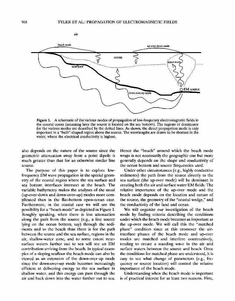
Figure 1. A schematic of the various modes of propagation of low-frequency electromagnetic fields in the coastal ocean (assuming here the source is located on the sea bottom). The regions of dominance for the various modes are described by the dotted lines. As shown, the direct propagation mode is only important in a "bulb"-shaped region above the source. The wavelengths are drawn to be shortest in the water, where the electrical conductivity is highest.

also depends on the nature of the source since the geometric attenuation away from a point dipole is much greater than that for an otherwise similar line source.

The purpose of this paper is to explore low- frequency EM wave propagation in the special geometry of the coastal region where the sea surface and sea bottom interfaces intersect at the beach. The

variable bathymetry makes the analyses of the usual (up-over-down and down-over-up) modes more complicated than in the flat-bottom open-ocean case. Furthermore, in the coastal case we will see the possibility for a "beach mode" as depicted in Figure 1. Roughly speaking, when there is less attenuation along the path from the source (e.g., a line source lying on the ocean bottom, say) through the sediments and to the beach than there is for the path between the source and the sea surface, regions in the air, shallow-water zone, and to some extent near- surface waters farther out to sea will see an EM

contribution arriving from the beach. In typical examples of a sloping seafloor the beach mode can also be viewed as an extension of the down-over-up mode since the down-over-up mode becomes increasingly efficient at delivering energy to the sea surface in shallow water, and this energy can pass through the air and back down into the water farther out to sea.

Hence the "beach" around which the beach mode

wraps is not necessarily the geographic one but more generally depends on the shape and conductivity of the ocean bottom and source frequencies used.

Under other circumstances (e.g., highly conductive sediments) the path from the source directly to the sea surface (the up-over mode) will be dominant in creating both the air and surface water EM fields. The relative importance of the up-over mode and the beach mode depends on the location and nature of the source, the geometry of the "coastal wedge," and the conductivity of the land and ocean.

We will organize our investigation of the beach mode by finding criteria describing the conditions under which the beach mode becomes as important as the up-over mode. We will call this the "matched phase" condition since at this crossover the air- interface phases of the beach mode and up-over modes are matched and interfere constructively, tending to create a standing wave in the air and surface waters between the source and beach. Once

the conditions for matched phase are understood, it is easy to see what change of parameters (e.g., frequency or source location) will control the relative importance of the beach mode.

Understanding when the beach mode is important is of practical interest for at least two reasons. First,

TYLER ET AL.: PROPAGATION OF ELECTROMAGNETIC FIELDS 969

potential navigation applications (such as for an autonomous underwater vehicle (AUV)) may require that the phase information of the EM field be interpreted. If the beach mode is important, however, the phases may be seen to arrive from the beach rather than from the source located farther out to sea, and this could be an obvious source of confusion. In this

case, it is desirable to know how to select the source location and/or frequency such that the beach mode is unimportant. For coastal underwater communications the phase information might not be important, but the desire may be simply to increase the signal strength at the receiver. In this case, it might be of interest that the beach mode will increase the shal-

low-water signal strengths beyond what would be obtained from just the up-over-down and down- over-up modes.

In the next section we give a brief description of the basics of EM propagation in a good conductor (read- ers familiar with this can skip this section). In section 3 we make theoretical estimates of the matched-

phase condition for idealized coastal geometries and give practical strategies for finding this condition for more complicated realistic cases. In section 4 we use a two-dimensional (2-D) numerical simulation to test the theoretically expected matched-phase condition and to illustrate the other ideas presented. Finally, in the last section we present our conclusions and describe some of the potential utility of coastal EM propagation.

2. EM Propagation in a Good Conductor Ocean water has an electrical conductivity ranging

from about 2 to 6 S/m. The conductivity of the underlying sediments may be as large as 0.1-1.0 S/m (for very wet sediments) or several orders of magnitude less than this. The air is essentially an insulator. We will be interested in EM effects within the coastal

region where all three media are present. We will mainly treat two-dimensional (2-D) problems involving a vertical/offshore slice through the coastal domain with variables and parameters along the coast assumed uniform. In the formulations we allow for

both motional and controlled impressed sources since both can be included in the same way.

2.1. Transverse Electric (TE) Mode

2.1.1. Formulation. To derive a governing equation for the electric field strength E (V/m), we start with two of Maxwell's equations:

OrB + V x E = 0, (1)

at(geE) +/xJ - V x B = 0, (2)

where B is the magnetic flux density (in teslas), J is the electric current density (A/m2),/x is the magnetic permeability (H/m), and • is the electric permittivity (F/m). We take the curl of (1) and the time derivative of (2) and combine to remove B:

OtOt(txeE) + ot(/xJ) + V x V x E = 0. (3)

We will assume that an induced electric current Ji and an impressed (controlled source) current Jp comprise the total electric current J - Ji + Jp. Ji is related to E by Ohm's law for a moving conductor'

Ji: cr(E + u x B)• cr(E + u x F) (4)

where u is the ocean velocity (m/s), o-is the electrical conductivity (S/m), and in arriving at the approxima- tion shown, we assume the total magnetic field B, which includes the secondary magnetic fields induced within the ocean, can be replaced by the very much larger Earth's main magnetic field F.

Using (4) in (3) gives

OtOt(tx•:E) + 0t(/xo-E) + V x V x E

: -Ot(la, cru X F + /XJp) (5)

with the sources appearing on the right-hand side of the equation.

Let us consider the case where o-is independent of time, the material media is not magnetic (/x - /Xo, where/x o is the vacuum magnetic permeability), and there are no variations in the y direction. The y component of equation (5) reduces to

- O,OtE + OrE - KV2E = OtJo (6)

where K - (/ZOO-) -• and we have defined E = E- y and Jo = (rru x F + Jp)-y (y is the unit vector in the y direction). Given the electric current Jo due to controlled and motional sources, the transverse electric field E is found using the appropriate boundary conditions.

2.1.2. Frequency domain. For a forcing current Jo with a sinusoidal temporal dependence of the form e -itøt (i - X/T- 1, co is the forcing frequency (per second), and t is time (seconds)), we seek solutions for E having a similar time dependence. (The physical quantities are understood to be the real parts of the


complex expressions.) After carrying out the temporal differentiation in (6), we have

V2E + t<2E = -itolXoJo (7) and

where

K 2= to2e/,o + itolXoO' (8)

is the complex wave number, or propagation constant. The behavior of the solutions to (7) will depend on

the relative importance of the real and imaginary parts of K. When displacement currents dominate conduction currents Ie/l >> 1, the real part of K is much larger than the imaginary part, and the solution is wavelike. When << 1 (conduction currents dominate), the homogeneous part of (7) becomes a diffusion equation. With the periodic forcing term included, however, the solution will still exhibit wavelike behavior.

To model (7) numerically, we would decompose it into two equations assuming E = E R + iEi, Jo = JoR + iJoI, and •2 = (•:2)R + i(•:2)i.

V2ER + (t<2)iEi = tolXoJoi + (t<2)iEi . (9)

V2Ei + (t<2)REi = --tolXoJoR -- (t<2)iER ' (•o)

In terms of (9) and (t0), the previous discussion can be stated as follows: Equations (9) and (t0) are wave equations coupled through conduction-current terms (involving (g 2)i); when the conduction current is small relative to the displacement current, (9) and (t0) are uncoupled wave equations; when the conduction current dominates, however, (9) and (t0) become "perfectly" coupled.

2.1.3. Plane wave solution. So far, in deriving (7), we assumed an axis of invariance (y). Now we also assume that there are no variations in the x

direction and consider plane waves propagating in the -z direction (z taken to be increasing upward from the sea surface, where it is zero). Physically, this could represent EM waves of ionospheric origin propagating into the ocean from the sea surface.

The solution to (7) for this case is

E = Eo ey/a cos(mz - tot) (•)

where E o is the value (which we take to be real) at the sea surface,

1/2

[(1 + Q-2)1/2 _ 111/2, (12)

m = to [(1 + Q-2)1/2 + 111/2. (13)

Above, Q = toe/o-, in older literature termed the "quality factor," measures the relative importance of displacement and conduction currents. (For periodic forcing, Q can also be thought of as the ratio of the relaxation time of the conducting medium to the period of the forcing, or the number of cycles the wave completes before it is attenuated to 1/e its value.) The parameters/5, m are related to g by K = +_ (m + i/a). Physically, m represents the (real) wave number, while a is the e-folding decay scale (also called the "skin depth").

We now discuss the results above using typical parameter values. The electrical conductivity of seawater ranges from about t to 6 S/m, and the relative electric permittivity is about 80 (Sr • 80; e = 8r8o • 7.1 x 10 -•ø F/m). Therefore, for forcing frequencies co << 109 Hz, we have Q << 1 and 15 -• = m - (•OtXotr/2) •/2. As we will further see, this constrains the forcing frequencies to an operational range which we take to be about 10 -2 to 10 2 Hz. At these frequencies the sediments and rock below the ocean (with tr > 10 -•) are also relatively good conductors, and the results above for seawater apply. (An implicit assumption has been that the electrical conductivity can be represented by its scalar "static" value. That is, it is assumed that the frequencies of interest are much lower than the natural frequencies of the microscopic oscilla- tions of the material medium and that the medium is

electrically isotropic. At light frequencies and higher the formulas presented here would give incorrect skin depths for the ocean of the order of millimeters. In fact, light propagates many meters in the ocean. The correct calculation would involve use of the general complex conductivity.) The conductivity of the lower atmosphere is highly variable and nonuniform but is about 12 orders of magnitude less than that of seawater. Also, because for air e • eo, Q-• << 1, 15 • 0, and m • •o(tXoeo)•/2 = toc -1 (or phase velocity = •o/m = Co (vacuum light speed), as expected for free space). The results for the electrical parameters in seawater and the sediments are extended in Table 1 and Table 2.

TYLER ET AL.' PROPAGATION OF ELECTROMAGNETIC FIELDS 971

Table 1. Sediment Electrical Properties (for Frequencies 10 -2 -• 10 2 Hz) Parameter Approximate Form Numerical Value

Conductivity o- Permittivity e Quality factor Q = Skin depth/5 Wave number m

Wavelength X - 2,r/m Complex wave number k Phase velocity c -

eo -• 80eo

(2/co/.ro o-) 1/2 (co/.ro o-/2) 1/2 2rr/5

_+(1 + i)m = +-(icol. roO') 1/2 (2co/cr/.ro) 1/2

10 -5 -• 1 S/m 8.854 x 10-12 F/m 5 x 10 -13 --> 5 x 10 -4 50--> 1.5 x 106 m 7 x 10 -7 --> 0.02 m -1 300--> 107 m

125•4 x 106m/s

2.2. Magnetic Vector Potential In the previous section we formulated the electro-

dynamic processes in terms of the electric field. This is useful since the electric field is one of the EM

quantities that is often measured. However, when we consider constructing a numerical model, the electric field has a complication since it can be due to two types of EM processes and a model of these processes must be understood and specified before the problem, together with proper boundary conditions, can be correctly formulated for computation. Specifically, the electric field can be written as

E: -OtA- V•, (14)

where A is the magnetic vector potential and 4> is the electric potential. Electric fields can be induced by EM time fluctuations (described by the first term on the right-hand side of (14)) but also can exist due to the establishment of spatial charge densities (the second term). This distinction should be better clari- fied for many problems using the electric field formulation with material media. In the case we will con-

sider in this paper, for example, of an alongshore line source located on the sea bottom off the coast, use of a 2-D transverse electric field formulation together with natural boundary conditions will implicitly imply that the alongshore spatial charge densities are uniform, and this is equivalent to assuming E - -0 t A. If

the case we are attempting to model is located inside a bay, for example, this may be a poor assumption since the alongshore electric field will be partially supported by alongshore spatial charge densities. If the line source is in electrical contact with the me-

dium, the alongshore spatial charge density assumption may also be incorrect because of resistivity effects. Next we will describe a formulation that is

more powerful than that based on the electric field (TE mode) and avoids the inherent ambiguities of the electric field formulation.

Maxwell's equations and Ohm's law for a moving conductor can be combined to give

OtA - u X V X A + V& - KI•2A

= -KV(V. A) - KO,(•Vq•)

where E]2[ ]=V2[ ]-Ot(la,•Ot[ ]).Thetrans- verse electric (TE) mode described in section 2.1 is just a special case of (15). This can be shown as follows. Under the Coulomb gauge, and assuming •, • are independent of time, the right-hand side of (15) vanishes. Allowing again for impressed motional and controlled sources Jo - rru x F + Jp, (15)becomes

OtA - u X V X A + V& - KI•2A = Jo/cr. (16)

We can obtain 2-D formulations as follows: Typi- cally, we can neglect motional self-induction because

Table 2. Ocean Electrical Properties (for Frequencies 10 -2 -• 10 2 Hz) Parameter Approximate Form Numerical Value

Conductivity cr Permittivity e - 80eo Quality factor Q = toe/or Skin depth/5 (2/cO/XoCr) 1/2 Wave number m (cO/XoCr/2) 1/2 Wavelength X = 2,r/m 2rr/5 Complex wave number k _+(1 + i)m - __+(icOp, oO') 1/2 Phase velocity c = to/m (2to/O.•o) 1/2

1 -• 6 S/m 7.0832 x 10 -1ø F/m 10 -11 -• 5 x 10 -7 25 -• 2500 m 0.04 -• 4 x 10 -4 1/m 160-• 1.6 x 103 m

65 -• 6.5 x 104 m/s

9'72 TYLER ET AL.: PROPAGATION OF ELECTROMAGNETIC FIELDS

the motionally generated magnetic field b = !7 x A << F. Also, we assume that owing to the small ratio of the vertical to horizontal ocean scales, the OyOy component of the diffusion term is negligible. Equation (16) becomes

1

OtAy q- Oyd)- gI•2Ay =-Jo. (17)

When we differentiate (17) with respect to time and assume OyCk = 0, we obtain an equation which is equivalent to the usual TE formulation (equation (6)) but with the source of the electric field unambigu- ously identified as Ey = -OtAy. Hence, for cases where it can be assumed that 0yqb = 0, the vector potential formulation might be viewed as similar to the TE formulation but more general since it allows for steady electric current sources.

3. Which Modes Dominate and Where?

As we discussed in the introduction, the study of propagation of EM energy over all but small distances in the coastal region is inherently a study of propagation along the indirect paths. That is, for regions except those very near the source, the dominant EM energy will arrive through indirect paths involving the sediments, air, or both (as in the beach mode presented in this paper).

The importance of the various modes (direct, up- over-down, down-over-up, and beach), which are shown schematically in Figure 1, depend on the parameters describing the sediment and water conductivity, the geometry of the coast, and the location and nature of the EM source (transmitter). Typically, the up-over-down mode will be important at least in the surface waters, and it is convenient to compare the importance of the other modes to this one. In the following, we will first make simple preliminary statements for the usual direct and down-over-up modes, and then we give greater attention to details in examining the beach mode. Many of these details also apply to the other modes.

Theoretical results from the previous section were used in making qualitative estimates of path attenuation for the various modes. These estimates, together with some allowance for spreading, were con- sidered in producing the schematic depicting the expected regimes of dominance for the coastal modes shown in Figure 1.

3.1. Direct Mode Versus Up-Over-Down Mode

As depicted in Figure 1, we see that for the example of a source (assumed here to be a line source parallel to the coast) located on the seafloor, the direct mode is important only within a "bulb"-shaped region above the source. The direct mode can dominate the up-over-down mode only within a range roughly less than the sum of the source and receiver depths. The bulb-shaped region is narrow toward the bottom because the down-over-up mode provides energy to the deep waters more efficiently since the path through the sediments is generally less resistive than that of the direct path through the water. The maximum width of the bulb is about an ocean depth.

If the source is located at the surface, the bulb is inverted and is narrower at the stem and wider near

the seafloor than the bulb shape shown. For a source at middepth the shape becomes more circular (but wider at the bottom).

3.2. Down-Over-Up Mode Versus Up-Over-Down Mode

The importance of the down-over-up mode relative to the up-over-down depends much on the location of the source in the water column. For a source at the

surface the down-over-up mode will never dominate because the sediments are more conductive than the

air. For a source at middepth the down-over-up mode will usually only be important at receiver locations which are below the level where the sum of the

receiver and source heights above the seafloor equals the sum of source and receiver depths.

When the source is located on the seafloor, the down-over-up mode can dominate over much of the water column. With poorly conducting sediments, this range may extend nearly to the sea surface. Usually, however, the up-over-down mode will remain dominant within the surface waters. The exception to this is if the variations in bathymetry are such that the receiver is in much shallower water than the source.

In this case, the down-over-up mode may dominate even in the surface regions (but only where the water is shallow), and the up-over-down mode is not important in this region.

We can attempt to better quantify these estimates by making comparisons of the EM attenuation along each path using simple ideas as presented in section 2. In this approach, the two modes are compared by simply comparing the number of skin depths along each path. It should be noted that this approach draws on ideas of plane wave attenuation (which are


not truly valid in these cases involving nonhomoge- neous conductivity), and similarly, no quantitative consideration is given to the geometric attenuation.

For a source a distance Ah above the sea bottom, the down-over-up mode is expected only to be dominant below levels where the height above the seafloor Az satisfies

Az • h - Ah - x/rrs/rrwr/2, (18)

where r is the horizontal distance to the source and o- s and o- w are the conductivities of the sediments and water, respectively. This follows from simple compar- ison of the resistance along the path down from the source, into the sediments, and back up, and the direct path through the water.

3.3. Beach Mode Versus Up-Over-Down Mode

The statements made above concerning the other modes are fairly intuitive and can be understood in simple terms using ideas of plane wave propagation and attenuation as presented in the last section. Neglected in this, however, are effects due to geometric attenuation (spreading) and the inhomogeneous conductivity. These effects become increasingly important for the beach mode and will be briefly con- sidered when discussing the importance of this mode.

As we will see later, the EM amplitudes in the shallow shore region can be larger than those closer to the source. While this can be partially understood as simply a convergence of the up-over-down and down-over-up modes near the beach, this is not a complete description. First, even when both of these modes are important and converge in the shallow- water zone, they must be in phase in this region in order to interfere constructively and give larger amplitudes. Second, part of the energy in this region is due to the beach mode, which describes energy which has passed through the sediments to the beach and then reenters the water. Below we will derive a

matched phase condition which simultaneously gives the conditions for which the up-over-down and down- over-up modes are in phase in the shallow water and beach region and describes when the beach mode becomes important.

3.3.1. Conditions for matched phase. If either the air or sediment modes operated separately, we would expect the EM phase in the air to be roughly uniform locally. This is because it is difficult for EM waves traveling out of a homogeneous region of a good conductor and into a poor conductor to show interference even when the waves arrive at the inter-

face with differing phase. This is because in the conductor the skin depth is of a small scale comparable to the wavelength. Any waves arriving at the interface that might have a phase different than the phase of waves taking the shortest path to the interface are necessarily weaker and unable to interfere effectively.

Considering a line EM source located on the sea bottom at depth h, simple geometric arguments suggest that the "source area" (the region through which the bulk of the energy arrives at the surface) for the air directly above the source is essentially a strip of sea surface of width of the order l, where

I=28w 1+ . (19)

For h << 8w, l = 28w, while for 8w << h, l = 2X/-•w h. Notice that an implicit assumption here is that l < d (where d is the distance between the source and beach), which requires that the frequencies used are not so low that the strip width l overlaps the land. Although much of the discussion below still applies for lower frequencies when l < d, it can be appreci- ated that the ocean geometry and various EM modes (in fact, even the presence of the ocean) become less important as the frequencies are decreased and the ocean dimensions become much less than the EM

wavelengths in the sediments or air. For the lowest frequencies we might even ignore the ocean and find reasonable solutions with a half-space model.

We can make an estimate of the frequency (which we will call •oa) below which the coastal geometry becomes unimportant by setting l in (19) equal to d and solving for the frequency using the relationship relating the skin depth to frequency given in Table 1. The result is

I•o rrwd 2 -• + 1 +

l•o O'w d2

-2

1 + 2 = (20) tZ o O'w d2

For d = 1000 m and o- w = 4.0 S/m, this requires frequencies less than about 0.25 Hz.

At the beach an estimate of the horizontal scale on

which the down-over mode feeds the atmosphere is estimated by the EM skin depth in the sediments. When we include this mode with the up-over-down mode, the phase in the air will no longer be uniform


except for the case where the waves following the path up through the ocean and the waves following the path through the sediments and beach arrive at the air in phase. (The fact that the two air/interface locations are separated in space would not be important for the low frequencies we consider since the air wavelengths are much greater than the domain of interest.) When waves arriving along both paths arrive at the air in phase, we will refer to this as matched phase. This will lead both to constructive interference and the tendency to create a standing wave in the air and near-surface waters between the source and

beach.

When discussing "constructive interference," we must keep in mind that the process is diffusive and only "wavelike" if the driving source is periodic. For similar reasons we cannot expect harmonics of the matched-phase condition; while it is true that if the ratio of the number of EM wavelengths along the two paths were an integer the arrival phases would match, energy from one path would now be significantly attenuated relative to the other. Hence the matched-

phase condition here also requires that the two paths give EM amplitudes of roughly comparable magnitude (they will not be precisely the same magnitude since the spatial attenuation and other factors along the two paths are not the same).

Now we will estimate the necessary conditions for matched phase. For this discussion we will assume that the source is located on the ocean bottom at

depth h. A simple matching of the two propagation travel times along each path would give the condition

rs d x/•s rw h •w 1, (21)

where h is the depth to the source and *s and *w are the travel times through the sediment and water paths, respectively. The quantity *s/*w (here set equal to 1 for the matched phase condition) is more generally a dimensionless number describing the relative importance of the beach mode to the up-over mode.

The condition given in (21) was restricted to the case where the sediment EM wavelength was small. This is because the EM energy traveling through the sediments must wrap around the beach to enter the air. However, the scale for this wrapping effect to occur should depend on the EM wavelength of the medium. Hence an improvement to the estimate given in (21) which increases d by an amount equal to one half the wavelength is

2 ) 1/21 d + rr = 1. (22) to/.•o rr s

Aside from perhaps better accuracy, the condition in (22) is also frequency dependent, allowing the possibility of tuning a system to attain matched phase (this also can be done by moving the source but might not be as convenient). Note, however, that this "tuning" capability has some important limits due to other considerations as described below.

Taking the other parameters as specified, we can solve (22) for ro = rOmp to obtain the following expression for the matched-phase frequency:

27r 2 romp-- (h •w - dx/-•s) -2 (h •w > dx/-•s ) (23)

/•o

The additional constraint below (23) stems from the fact that the choice of the source frequency can only be used to increase the beach-mode path from the minimum path given by the source-to-beach distance. For example, assuming the source is located on the sea bottom, if we consider a coastal-wedge region, the condition above tells us that to have matched

phase the slope (h/d) must be sufficiently steep, satisfying

h/d > x/crs/crw. (24)

Provided (24) is satisfied, (23) can be used to tune the system to attain matched phase. Then, when frequencies greater than rOmp are used, a stronger beach mode arises; for lower frequencies the direct up-over path begins to dominate.

Above we have discussed the conditions for which

the phase and amplitudes of the EM waves arriving at the beach, and at the air directly above the source, are similar. We also stated that when this condition

occurs, the EM phase between these points in the air will show a standing wave node (described by a region of closed phase contours). (In fact, it is not possible to produce a standing wave node in the air unless the beach mode is important. In contrast, when the up-over-down and down-over-up modes are the important modes, a standing wave node can only occur below the sea surface in the water. Hence the location

of the standing wave node is an indicator of which modes are important.) This statement must now be qualified since its truth depends on the particular shape of the sea bottom and the source frequency used.


If the shape of the sea bottom is such that it drops off quickly from the beach and then begins to level out approaching the source (positive curvature), the matched-phase criteria should be as stated above. If, however, the sea bottom has negative curvature, paths connecting the sediments and air through the shallow-water zone also become important. Essen- tially, the EM waves coming through the sediments wrap around and up to the air somewhat sooner (offshore) than at the geographic beach.

A realistic sea bottom can be quite complicated. Provided, however, that the sea bottom continually deepens in moving from the beach to the source location, we can summarize that when the bottom shape has an effect, it is to move the effective beach location offshore. Because of these sea bottom shape effects, for many realistic cases the frequency that gives a standing wave node in the air region between the source and beach will be, in practice, somewhat lower than the matched-phase frequencies defined above.

There are some other effects we have not included.

One is that due to the differences in geometric attenuation for the two paths. As we described above, l given by (19) is an estimate of the scale describing the radiation to the atmosphere above the source, while a similar scale for the radiation at the beach is

given by the sediment skin depth. These scales, which are not generally equal, should be important in describing the geometric attenuation away from the two radiating surfaces. Hence, while this might not formally affect the matched-phase criteria, we do expect that it will affect the location of the standing wave node above the sea surface and will have an

effect on the relative magnitudes. Finally, while the up-over mode propagates from

the source to the sea surface through a rather homo- geneously conductive ocean, the propagation path through the sediments involves not only the conductivity inhomogeneities of the sediments, but also, propagation along this path occurs near the interface of a good conductor (the ocean), and energy is lost to this interface.

A strategy for a practical determination of the matched-phase frequency (if need be) is then to use the criteria given by (23) to make the initial guess and then, if necessary, compensate for the bottom shape effects by lowering the frequency until the standing- wave node is attained in the air between the source

and beach. While in the numerical cases we present next, consideration of the effects due to the differing

spatial attenuation scales and sediment/ocean interface losses does not appear crucial in producing the predicted standing-wave node, we do see beach mode amplitudes slightly reduced relative to those of the up-over mode.

3.3.2. When is the beach mode important? In this section the conditions under which the beach

mode becomes important have been described in detail, together with various caveats that we will now relax to give a simple but loose estimate of the dimensionless number describing the relative importance of the beach mode. The appropriate dimensionless number 'rw/'r s was described in (23) and is extended here to include sources which are not on the

seafloor but are raised by a height Ah above the seafloor. The result is

rw • a + (25)

where t5 s - (2/tOtXoO's) •/2 is the skin depth in the sediments. The beach mode is unimportant only when 'rw/'r s is either <<1 or negative.

The beach mode, when important will usually only be important in waters near the surface. This is because when the beach mode is important, the down-over-up mode (which feeds the beach mode) must also be important. In these cases, the down- over-up mode will dominate over at least the lower half of the water column.

3.3.3. The beach mode acting in reverse. We have concentrated so far on sources located on or

near the seafloor. If the source is at or near the

surface, the beach mode previously discussed is not important, but a new version (one with a reversed sense of propagation) can be expected. In this case, it is the near-seafloor locations rather than the surface

locations which are most affected.

In this reversed beach mode, energy travels from the source to the beach, seaward through the sediments, and reenters the water through the seafloor. Since this version does not first travel through the sediments, it can be more effective at delivering EM energy to the nearshore bottom waters. Another difference is that this reversed mode will have little

competition from the down-over-up mode (compared with the competition for the usual beach mode from the up-over-down mode). In this case, no standing wave in the seabed is expected. Rather, any competition (for influence near the sea bottom) comes again from the up-over-down mode.


In the simplest estimate the reversed beach mode will be important relative to the up-over-down mode for receiver locations where

hr - Ahr o'•• --> (26) dr + Ahr '

where d r is the distance of the receiver to the beach, h r is the water depth at the receiver, and Ah r is the height of the receiver above the seafloor.

The reversed beach mode would appear then to be dominant throughout the near-seafloor region (Ah r • 0) when the slope of the seafloor is greater than V'•rs/•r w. The up-over-down mode will still generally dominate in the upper half of the water column. Note that in this last case, assuming a uniform slope, the condition for the importance of the reversed beach mode is the same as the condition

(21) for the earlier "regular" beach mode. This is because with a uniform slope, hr/d r = h/d describing the bottom source.

4. Numerical Validation

Now we will consider a few numerical examples that will serve both to illustrate the coastal EM modes

and to validate some of the theoretical conditions, particularly that of matched phase, derived in the last section. A periodic (e-itot) and infinitely long electric line current of unit amplitude (1 A) lies on the seafloor and is parallel to the coast. There are assumed to be no alongshore variations in the various parameters as well as the spatial charge densities (so the alongshore component of V0 is zero). Physically, this model is appropriate for a source where the source electric currents are insulated from the seawa-

ter or where the galvanic electric currents are neglected relative to the induced currents. The alongshore (y axis) component of the electric field is then simply Ey = -OtAy , and solutions for the 2-D equation (17) for Ay can be easily used to obtain the magnetic and alongshore electric fields.

The value used for o- s should roughly reflect the average sediment conductivity over a sediment depth of about an EM wavelength (hence the value that should be used can be frequency dependent), or, if the distance between the source and beach is smaller

than the skin depth, this scale for averaging the conductivity might be used. The conductivity of the continental margins is usually much more complicated than that of the deep-sea floor. While there may

be a very thin conductive layer of porous sediments near the sea bottom, deeper the conductivity of the continental rock may be several orders of magnitude less. Furthermore, the continental shelves are regions of intense geological activity, and the inhomogeneities in the conductivity will often preclude a 1-D description of the conductivity below the ocean. Be- cause of this and the wide diversity of continental shelf types, it seems that an appropriate range for the average conductivity o- s required here could be between o- s = 1 S/m (for a source close to the beach over very porous and thick sediments) and o- s : 10-5 S/m (for a source distant from the beach and/or over resistive continental rock with little or no sedi-

ment layer). The basis of the finite element numerical solver (partial differential equation, two-dimensional) we use to obtain solutions for Ay has been described by Sewell [1985].

For the first example we will consider the case of relatively high sediment conductivity (o- s - 0.1 S/m) for which the up-over-down mode dominates all regions except those very near the source. Through- out this paper we will take the seawater conductivity to be o- w - 4 S/m. We will assume here that the source operating at 250 Hz is located on the sea bottom 1 km away from and parallel to the beach and that the sea bottom has the simple flat-bottom geometry shown in Figure 2. We plot solutions for Ey = iooAy in Figure 2. In Figure 2a we plot the base-10 log of the magnitude, and in Figure 2b we plot the phase. The source is located at x = 0 m, y - -100 m, while the beach is located atx - -1000 m,y - 0 m. Simple Neuman boundary conditions are imposed at the edges of the domain (x, y - + 10 km). The water region is shown shaded. Superimposed on these figures is a line below which the equality/inequality of (18) is satisfied. This line gives the predicted separa- tion between the regions of dominance of the two modes and is in fair agreement with the solution. This can be seen by noticing that the solution phase lines which indicate down-over-up dominance appear at an angle to the seafloor (as opposed to the up-over-down phases, which are parallel to the sea surface) are confined to the predicted region below the line drawn. Also, in a bulb-shaped region above the source the phase lines describe the important direct mode, as predicted.

To test the matched-phase criteria derived in the previous section, we will first consider a flat-bottom ocean rising steeply to the beach as a wall (as in the last example). In this case, the matched-phase fre-


5O

0

-50

-100

-150

-2OO -151

Iog10(E (V/m)) -8.26

•. '•""•"--"•-'•'•""---• ..... • ..... :' 'i'•. ,••,•'--'i'•.•--• •".'•" :• .... •'•'- ................. •'•i•i •..•'•.:"-• .... •':.'I-'

1

t0 - 1000 -500 0

distance to source (m) a

phase (degrees)

-100

-150

-200 - -1500 -1000 -500 0

distance to source (m) b

Figure 2. (a) The log-10 magnitude of the electric field and (b) the phase due to a line source of frequency 250 Hz on a rectangular coastal sea bottom of high conductivity (rr s -- 0.1 S/m). The superimposed bold lines denote the regions below which the down-over-up mode is theoretically expected to dominate. To obtain decibel scale for amplitudes, multiply by 20.

quency should be given by (23) without need of further corrections (e.g., bottom shape). The sediment conductivity is crs = 0.01 S/m. Condition (23) then gives the matched-phase frequency as OOmp = 15 70.8 rad/s = 250 Hz.

The results for the phase shown in Figure 3b

indeed indicate a standing-wave node in the air between the source and beach, as predicted (if the figure is extended farther upward, the phase contours join to form a region of closed phase contours describing the node).

In the next example, we consider the wedge geom-


log 10(E (V/m)) 5

.............. *• ..... ..•-•.-•.•E ...... • ß • •-• ............. • ....... •%• .................. :•. • •:• • • • . :>' -:• ..... • ...... ...•.•... --' •. • .... ---.:. '• ....... - -

• ........ • •-• ............ •....-.••.•••••••••.•••,,••••,•.:•..,....:. •.,•,.••.:•...:.•. > •:5 •

-150[ ,/ / , .......... / / I

- 1500 - 1000 -500 0 distance to source (m)

a

5O

-2OO -1500

-50

-100

-150

phase (degrees)

,.-., ]•l• 60 -6o o

/

/ - 1000 -500 0


Figure 3. Same as in Figure 1 except sediment conductivity is 0.01 S/m. This case shows that the beach mode is important, particularly in determining the phase field in the surface waters.

etry whereby the ocean bottom slopes uniformly from the beach to the source (and continues on with the same slope to the offshore boundary, where again, Neuman boundary conditions are imposed). The rest of the geometry is the same as in the last example. Since the source depth and distance to the beach are the same as in the last problem, the predicted

matched-phase frequency without corrections for the ocean bottom shape is again 250 Hz (the condition (24) is also satisfied as required). The results are shown in Figures 4a and 4b. Indeed, a node appears in the air, demonstrating that both the up-over and beach modes are important. Note, however, that the node appears farther seaward relative to the case


Iog10(E (V/m)) ß -• me,_ _7 19

i '-t J'•dV I ......... ' ' -- I

7.56

................................... ;. •..,, :•..• .......................... ..................................... o. u.w•!.•,..•,....•.:,..,..•..,.,,:•,....,,.,.•..:...,.:.;,•., ........... •...:,,.,: •.• ......... •.:•>.•:•.• ..•.• ,:...•:,•.• ....... ...... • 6.68

36 -50

-1oo / / / 05

-150

-200 -1500 -1000 -500 0

distance to soume (m) a

phase (degrees)

' 0 60 -2' 0 •0

0 •:•d i / /

30 0 -lOO

30

-150

-200 ...... - 1500 - 1000 -500 0


Figure 4. (a) The log-10 magnitude of the electric field and (b) the phase due to a line source (250 Hz) on the coastal sea bottom for the case of a sloping sea bottom. The sediment conductivity is 0.01 S/m. To obtain decibel scale for amplitudes, multiply by 20.

shown in Figure 3. This indicates a slightly dominant beach mode phase and can be understood from the arguments given earlier related to the bottom shape since the wedge (with zero bottom curvature) has less bottom curvature than the case in Figure 3 (which has positive curvature).

Regarding the amplitudes, the increase of energy in the shallow zone for this case can, of course, be partially understood as simply due to the down- over-up mode being more effective in shallower water. These large shallow-water amplitudes, however, are also due to the fact that the matched-phase


-6

-6.5

-7

-7.5

o -8.5

-9

-9.5

-lo

i i

i

i

/

/

/

/

-10.5 ; 2•00 -10•00 • • • • • -1600 -14 0 -1 -800 -600 -400 -200 0 200

distance to source (m)

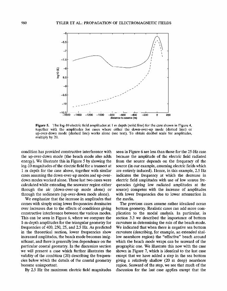
Figure 5. The log-10 electric field amplitudes at 1 m depth (solid line) for the case shown in Figure 4, together with the amplitudes for cases where either the down-over-up mode (dotted line) or up-over-down mode (dashed line) works alone (see text). To obtain decibel scale for amplitudes, multiply by 20.

condition has provided constructive interference with the up-over-down mode (the beach mode also adds energy). We illustrate this in Figure 5 by showing the log-10 magnitudes of the electric field for a transect at 1 m depth for the case above, together with similar cases assuming the down-over-up modes and up-over- down modes worked alone. These last two cases were

calculated while extending the seawater region either through the air (down-over-up mode alone) or through the sediments (up-over-down mode alone).

We emphasize that the increase in amplitudes that comes with simply using lower frequencies dominates over increases due to the effects of conditions giving constructive interference between the various modes.

This can be seen in Figure 6, where we compare the 1-m-depth amplitudes for the triangular geometry for frequencies of 400, 250, 25, and 2.5 Hz. As predicted in the theoretical section, lower frequencies show increased amplitudes, the beach mode becomes insig- nificant, and there is generally less dependence on the particular coastal geometry. In the discussion section we will present a case which further illustrates the validity of the condition (20) describing the frequencies below which the details of the coastal geometry become unimportant.

By 2.5 Hz the maximum electric field magnitudes

seen in Figure 6 are less than those for the 25-Hz case because the amplitude of the electric field radiated from the source depends on the frequency of the source (in our example, assuming electric fields which are entirely induced). Hence, in this example, 2.5 Hz indicates the frequency at which the decrease in electric field amplitudes with use of low source frequencies (giving low radiated amplitudes at the source) competes with the increase of amplitudes with lower frequencies due to lower attenuation in the media.

The previous cases assume rather idealized ocean bottom geometry. Realistic cases can add more complication to the modal analysis. In particular, in section 3.3 we described the importance of bottom curvature in determining the role of the beach mode. We indicated that when there is negative sea bottom curvature (describing, for example, an extended shallow nearshore region) the "effective" beach around which the beach mode wraps can be seaward of the geographic one. We illustrate this now with the case shown in Figure 7, which is identical to the last case except that we have added a step in the sea bottom giving a relatively shallow (20 m deep) nearshore region. Seaward of the step, we see that much of the discussion for the last case applies except that the


-5.5

-6.5

-7.5

-8.5

-9 -1600

2.5 Hz

-1 O0 -1 O0 -800 -600 -400 -200 0 200 distance to source (m)

Figure 6. The log-10 magnitudes of the electric field at 1 m depth for four source frequencies for the case similar to that of Figure 4. Only for the lowest frequencies do the amplitudes decrease monotonically away from the source. To obtain decibel scale for amplitudes, multiply by 20.

beach mode now wraps through the shallow water near the step rather than at the geographic beach. Within the shallow zone, however, the situation is more complicated and illustrates the necessary consideration that must be given to the seafloor shape when energy arriving through the sediments is involved.

5. Summary and Discussion We have attempted to describe the propagation

modes of EM energy in the complicated geometry of the coastal wedge. In the coastal waters and sur- rounding sediments and air, EM energy can travel along at least four different paths. The first is simply a direct path through the water between the source and receiving position. This path is usually only important very near the source. Two other modes are the well-known up-over-down and down-over-up modes. A fourth mode, which is specific to the coastal

geometry, involves a path through the sediments, into the air, back seaward, and in the case of a submerged receiver, back into the water. In the air, EM energy appears to be radiated from a patch of ocean directly above the source and a patch of land/water near the beach. Depending on the relative importance of the beach and up-over modes, EM waves in the air and surface waters can be observed to have advancing phases either toward the beach or away from it (though in the surface waters the phase advance is still dominantly vertical and from the surface).

In section 2 we reviewed the theory of EM propagation in a domain including good conductors and derived a useful formulation involving the vector potential which allows for general (including steady and motional) sources. Useful parameters such as the skin depth were derived for propagation in a homogeneous conductor, and these parameters were useful in indicating which coastal modes will dominate. However, the coastal region is certainly not a homogeneous region, and various other factors needed to be included in the analyses. In particular, while phase propagation and amplitude attenuation are related in a simple manner for a homogeneous medium, this is not true for the case of the coastal case involving propagation along several indirect paths.

For low frequencies, propagation becomes less dependent on the details of the coastal geometry. In (20) we gave the cutoff frequency below which the coastal geometry becomes unimportant. In the examples presented assuming a source on the seafloor at 100 m depth and 1 km away from the beach, this cutoff frequency is 0.25 Hz.

Very near the source the EM energy will be dominated by that due to propagation directly through the seawater. Farther away, energy arrives by one or more of the other modes, and we have attempted to describe when and where each of these modes are important. We gave a dimensionless number (equation (25)) describing when the beach mode is expected to be important. These conditions giving an important beach mode involve not only the geometry and conductivities of the coastal region but also the source frequency.

In section 4 we gave numerical results for a few cases which verified the theoretical predictions regarding the behavior and importance of the various modes. The operating frequencies for a practical problem will be constrained by the high attenuation of high frequencies. Low frequencies, on the other hand, aside from being undesirable because of the


log 10(E (V/m))

-7 47 -7.

-so -oo

-150

-200 -1500 -1000 -500 0

distance to source (m) a

phase (degrees)

6 0 0

"• - 1 O0 30 ..... •"•*•:•

-150 -30

-200 • • ....... •' ......... • - 1500 - 1000 -500 0


Figure 7. (a) The log-10 magnitude of the electric field and (b) the phase due to a line source of frequency 250 Hz for a complicated wedge with step. To obtain decibel scale for amplitudes, multiply by 20.

low bit rate (in communication applications), will show a decreased dependence on the specific ocean geometry. This creates an EM field which is easier to interpret (and potentially useful for navigation), but the gradients in the amplitude and phase are now smaller. Because of this, typical operating frequencies

would likely fall in the range between about 10 -2 and 10 3 Hz.

The results we have presented assume highly idealized cases and should be regarded with caution when considering more complicated practical applications. Still, we will finish by giving a rough descrip-


tion of some potential applications of coastal EM propagation and, in particular, describe how to strengthen or weaken the various propagation modes discussed.

5.1. Applications (Navigation) Where the Phase Field Must Be Interpreted

In applications such as underwater navigation, where it may be desirable to have an EM phase field which can be interpreted simply, we would likely want to choose the configuration such that the beach mode can be neglected. In fact, the simplest configuration would involve low frequencies such that the particular nature of the sea bottom becomes unimportant. The condition describing this "sufficiently low" frequency was given in (18). For a case similar to that shown in Figure 7, this frequency (calculated using (20) is •og = 0.25 I-Ii; the corresponding solutions for this low frequency are shown in Figure 8 together with solutions for a higher frequency of 25 Hi. Operating together, these two frequencies might be used to give a navigation grid which is not critically dependent on the details of the geometry and is nearly orthogonal, at least near the sea bottom. Because the vertical

coordinate might be easily observed by other means (e.g., a pressure sensor), one of these low frequencies alone might suffice to describe the range from the source. The grid of phase lines shown in Figure 8 can be made more orthogonal by increasing the higher of the two frequencies (25 Hi), but this comes at the expense of having more dependence on the details of the coastal geometry.

The simplest higher-frequency phase field to interpret would be one for which the up-over-down mode dominates (but in this case a source near the surface may be required). The up-over-down mode will be easier to interpret since the phase lines propagating from the "flat" sea surface are not deformed by the sea bottom. To illustrate this, we show in Figure 9 a case identical to that shown in Figure 7 except that the source is located at the sea surface. We should

note that the phase very near the bottom and in the near-beach region can be affected by the reversed beach mode in this case, in the same way a bottom source and associated beach mode can affect the

phase in the near-surface and near-beach region. This higher-frequency surface source and associ-

ated up-over-down mode will typically just show phase propagation downward from the sea surface and alone would not likely satisfy the system needs (of creating a navigation grid, for example) unless more

than one frequency or source was used or the EM information was combined with compass, altimeter, pressure, or other information. (We note that while the up-over-down mode would primarily only give grid information that describes depth (which can be easily obtained from a pressure sensor), a grid with the down-over-up mode would be more related to distance above the seafloor.) Moreover, for many applications it may be more practical to locate the source on the seafloor. In this case, the down-over-up mode would be involved. In any case, the down- over-up and up-over-down modes will usually have phases that are easier to interpret than the beach mode, and (if operations above or near the sea surface, or very near the beach are required) we would likely want to select the system configuration to deemphasize this mode. How do we do this?

As described in previous sections, the importance of the beach mode can be controlled to some degree by the choice of source frequency. The most practical and safest way of removing this mode, however, is simply to choose the configuration such that beach mode is not important for any frequency. This can be done by referring to the dimensionless number given in (25).

5.2. Underwater Communications

Finally, we can try to give a rough evaluation of the potential for communications applications in the coastal region when the beach mode is included. A similar evaluation was performed for the case of the subcrustal waveguide by Chave et al. [1990]. These authors gave estimates for a proposed standard model of the substructure conductivity. A standard model for the coastal region does not exist and may not be attainable. Nonetheless, we can present some estimates that may give a general idea of the communications potential using EM waves in the coastal region.

We consider the case shown in Figure 4 and envision the source being used as a transmitter to communicate with an AUV in the shallow region close to shore. We will assume the source current to

be 100 A. We will calculate the signal-to-noise ratio at the receiver location assuming, for simplicity, that at the source frequency here of 250 Hz, the dominant noise is due to amplifiers and the electrodes and is of order 1 nV/m per •. (At lower frequencies the noise due to motional and telluric currents will cer-

tainly become important.)


Iog10(E (V/m)) , -6.23

001 , / /

, ' ' •, ' ..... / 6.18 -200 -1500 -1000 -500 0


50

--- -50

(D

i- -100

-150

-2OO - 15OO

phase (degrees) ...... i I I

40.2

157.7 ....... ""*"'•' '"*' '

-1000 -500 0

distance to soume (m) b

40.2

Figure 8. (a) The log-10 magnitude of the electric field and (b) the phase due to a line source of frequency 0.25 Hz for a complicated wedge with step. Shown also are similar plots for magnitude (Figure 8c) and phase (Figure 8d) for a frequency of 25 Hz. As predicted, the case of 0.25 Hz does not depend on the details of the coastal geometry. The case of 2.5 Hz (not shown) is also fairly independent, and frequencies of 0.25-2.5 Hz could be used to determine range for navigation applications. The case of 25 Hz is clearly too high to determine range since the phase field becomes too dependent on the shape of the sea bottom. These higher frequencies, however, could provide information about the height above the seafloor and when used in combination with a lower frequency would produce a navigation grid. To obtain d½cib½l scale for amplitudes, multiply by 20.

TYLER ET AL.- PROPAGATION OF ELECTROMAGNETIC FIELDS 985

5O

-'-" -50 E

i -100

-150

-200 - 1500

log I O(E (V/m))

' ' -7 6 ':

_

i

- 1 ooo -5oo o

distance to source (m) c

phase (degrees)

-2O -3O

.......

5'_

-150

-200 - 1500 - 1000 -500 0

distance to source (m) d

Figure 8. (continued)

With the same notation as Chave et al. [1990] the power signal-to-noise ratio is

.4 2 SNR: -- (27)

4S, bf

where,4 is the source amplitude at the receiver, Sn is the noise spectral density, and Af is the bandwidth.

Estimates of the EM noise due to ionospheric

currents, microseisms, wind waves, and swell are given by Chave and Cox [1982]. The strongest noise is in shallow water since the externally induced electric currents are attenuated with depth. Also, the effects are stronger for the lower frequencies, having an electric field power spectral density S n of about 10 -14 to 10 -15 (V/m)2/Hz at 100 m depth and at 10 -2 Hz, and decrease to about 10 -22 (V/m)2/Hz at 10 Hz.


50

0

-5o-

-100 -

-150 -

-200 -1500

Iog10(E (V/m))

..... _.r//••-••• , .86 ...... • .4; - -•,':.,ii ! ............... ••• • . •••.• ..... ,,,• .......

- 1000 -500 0


50

-50

-1001

-150

-2o0 -1500 - 1000


phase (degrees)

.................. . ..

6 , -30 -40

-500 0

b

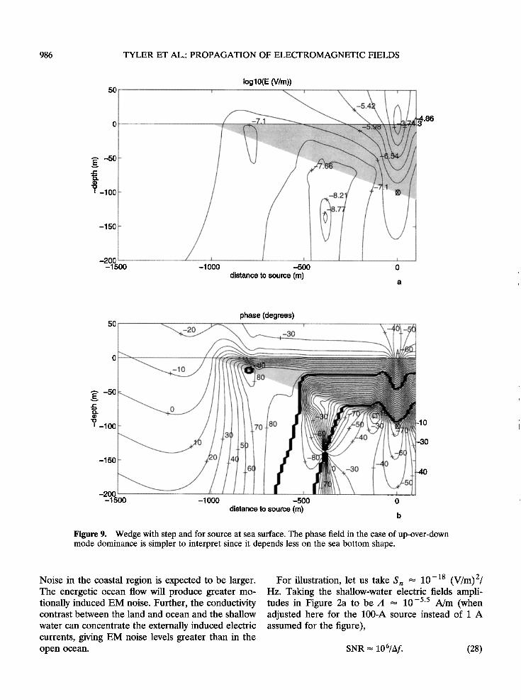
Figure 9. Wedge with step and for source at sea surface. The phase field in the case of up-over-down mode dominance is simpler to interpret since it depends less on the sea bottom shape.

Noise in the coastal region is expected to be larger. The energetic ocean flow will produce greater motionally induced EM noise. Further, the conductivity contrast between the land and ocean and the shallow

water can concentrate the externally induced electric currents, giving EM noise levels greater than in the open ocean.

For illustration, let us take S• = 10 -18 (V/m)2/ Hz. Taking the shallow-water electric fields amplitudes in Figure 2a to be A = 10 -5'5 A/m (when adjusted here for the 100-A source instead of I A assumed for the figure),

SNR = 106/Af. (28)


This ratio (which obviously remains large even for the largest Nyquist bandwidth) may suggest good possibilities for shallow-water EM communication at these frequencies, even for less favorable cases involving smaller source strengths, greater distance to the beach, higher sea floor conductivity, or increased geometric attenuation from realistic 3-D sources and receivers.

The signal strengths above are somewhat optimistic since they are calculated from our results assuming a line source. More realistic sources (e.g., a dipole source) will generally show faster spatial attenuation away from the source.

Also, we emphasize that the EM noise in the coastal region is expected to be larger than in the open ocean and probably quite regional. Aside from the usual near-surface noise sources (e.g., Schumann resonances) which will generally be present in the ocean, there may also be large artificial noise sources as well as concentration effects due to the coastal

conductivity contrast. As pointed out by a reviewer, the nature of the

noise source will also affect the relative importance of the various modes for a practical application. For example, in regions where atmospheric noise levels are large, the down-over-up mode may become more practical than other modes because it is somewhat shielded by the conductive water layer.

Acknowledgments. This study was conducted with sup- port from the Office of Naval Research under grant N00014-96-1-0246.

References

Bubenik, D. M., and A. C. Fraser-Smith, ULF/ELF electromagnetic fields generated in a sea of finite depth by a submerged vertically directed harmonic magnetic dipole, Radio Sci., 13, 1011-1020, 1978.

Chave, A.D., and C. S. Cox, Controlled electromagnetic sources for measuring electrical conductivity beneath the oceans, 1, Forward problem and model study. J. Geophys. Res., 87, 5327-5338, 1982.

Chave, A.D., S.C. Constable, and R. N. Edwards, Electrical Exploration Methods for the Seafloor, vol. 2, chap. 12, pp. 931-965, Soc. of Explor. Geophys., Tulsa, Okla., 1988.

Chave, A.D., J. R. Booker, C. S. Cox, P. L. Gruber, L. W. Hart, H. F. Morrison, J. G. Heacock, and D. Johnson, Report of a workshop on the geoelectric and geomagnetic environment of the continental margins, technical report, Scripps Inst. of Oceanogr., Univ. of Calif., La Jolla, 1990.

Inan, A. S., A. C. Fraser-Smith, and J. O. G. Villard, ULF/ELF electromagnetic fields generated along the seafloor interface by a straight current source of infinite length, Radio Sci., 21,409-420, 1986.

Moore, R. K., and W. E. Blair, Dipole radiation in a conducting half-space, J. Res. Natl. Inst. Stand. Technol., 65D, 547-563, 1961.

Petitt, R. A. J., J. H. Filloux, H. H. Moeller, and A.D. Chave, Instrumentation to measure electromagnetic fields on the continental shelves, Proc. IEEE, 1, 1164- 1168, 1993.

Sewell, G., Analysis of a Finite Element Method.' PDE/ PROTRAN, 154 pp., Springer-Verlag, New York, 1985.

T. B. Sanford, Applied Physics Laboratory, University of Washington, 1013 NE 40th Street, Seattle, WA 98105. (e-mail: [email protected])

R. H. Tyler, Institut fuer Meereskunde Abteilung Theo- retische, Duesternbrooker Weg 20, 24105 Kiel, Germany. (e-mail: [email protected])

M. J. Unsworth, Geophysics Department, University of Washington, Box 351650, Seattle, WA 98195-1650. (e-mail: [email protected])

(Received September 22, 1997; revised February 12, 1998; accepted March 6, 1998.)

propagation of electromagnetic fields in the coastal ocean...

Documents