~haptrr 1

GLOBAL POSmONlN6 SYSTf:M IN NAVIGATION AND

M£TEOROL06V

1.0 History of Navigation Systems

Navigation is a very ancient skill or art of planning, reading, and controlling the

movement of a craft or vehicle from one place to another. The word navigate is derived

from the Latin roots navis meaning "shipll and agere meaning IIto move" or "to direct". All

navigational techniques involve locating the navigator's position compared to known

locations or patterns. Fundamental navigation skill requires usage of our eyes, good

judgment ability and landmarks for moving from one place to another. However, in some

cases where a more accurate knowledge of our position, intended course, or transit time to a

desired destination is required, navigation aids other than landmarks are used. Methods of

navigation have changed through history. Each new method has enhanced the navigator's

ability to complete his voyage. One of the most important judgments the navigator must

make is the best method to use. A few types of navigation methods are listed below:

1. Pilotage: Essentially relies on recognizing landmarks to know the position. It

involves navigating in restricted waters with frequent determination of position relative

to geographic and hydrographic features.

2. Dead reckoning: Relies on a prior position, along with some form of heading

information and some estimate of speed.

3. Celestial navigation: Uses time and the angles between local vertical and celestial

objects (e.g., sun, moon, or stars). It involves reducing celestial measurements to lines

of position using tables, spherical trigonometry, and almanacs.

4. Radio navigation: Uses radio waves (from artificial source) to determine position by

either radio direction finding systems or hyperbolic systems, such as Decca, Omega and

LORAN-C. The latest satellite based radio navigation includes the Global Positioning

System (GPS).

2

5. Inertial navigation: Relies on the information on initial position, velocity and

attitude; thereafter measures the real time attitude and accelerations. A brief account

of this system is presented in the next section.

1.1 Inertial Navigation

Inertial Navigation System (INS) operates on the basis of Newton's laws of motion.

Newton's fIrst law of motion states that a body will continue to be in the state of rest or

moving with uniform velocity unless acted by an external force (inertia). The sensors used in

this system makes use of the property of inertia to measure accelerations and turn rates in a

fixed reference frame (an inertial reference frame) in which Newton's laws of motion are

valid. Once the acceleration is measured, it would be possible to calculate the change in

velocity and position by performing successive integrations of the acceleration w.r.t. time.

Since only changes in position and velocity are obtained using measurements, the

determination of initial position and velocity are very crucial in accurate navigation by INS.

The inertial sensors measure the vector-valued variables, rotation rate and acceleration,

usmg:

(a) Gyroscopes: These are sensors for measuring rotation; e.g. rate gyroscopes measure

rotation rate, and displacement gyroscopes measure rotation angle.

(b) Accelerometers: These are sensors for measuring acceleration. However, accelerometers

cannot measure gravitational acceleration.

Broadly, INS consists of two sections:

(a) An inertial measurement unit (IMU) or inertial reference unit (IRU) containing a cluster

of sensors: accelerometers (usually three) and gyroscopes (also three in number). These

sensors are rigidly mounted to a common base to maintain the same relative orientations.

(b) Navigation computers (one or more) which calculate the gravitational acceleration (not

measurable by accelerometers) and doubly integrate the net acceleration to maintain an

estimate of the position of the host vehicle.

The two systems of IMU are Gimbals and Strapdown for the INS. Gimbals have been

used for isolating gyroscopes from rotations of their mounting bases since the time of

Foucault. They have been used for isolating an inertial sensor cluster in a gimbaled IMU

since about 1950. At least three gimbals are required to isolate a subsystem from the host

vehicle rotations about three axes, roll, pitch, and yaw. A fourth gimbal is required for

3

vehicles with full freedom of rotation about all three axes: such as high-perfonnance

aircraft. In Strapdown type of INS, the inertial sensor cluster is "strapped down" to the

frame of the host vehicle, without using intervening gimbals for rotational isolation.

Strapdown INS generally requires more powerful navigation computers than their gimbaled

counterparts as this system computer must integrate the full (six degree of freedom)

equations of motion to estimate the position.

The main advantages of INS over other navigation systems are, (1) it is autonomous

and does not rely on any external aids or on visibility conditions, (2) it can operate in tunnels

or underwater as well as any where else, (3) it is inherently well suited for integrated

navigation, guidance, and control of the host vehicle, (4) its IMU measures the derivatives of

the variables to be controlled (e.g. position, velocity, and attitude) and (5) it is immune to

jamming and inherently stealthy, because it neither receives nor emits detectable radiation

and requires no external antenna which could be detected by radar.

The disadvantages of INS are that the mean-squared navigation errors increase with

time. The Acquisition, Operation and Maintenance costs for INS are order of magnitude

larger than that in radio navigation aids like GPS. The INS weight which is generally high

has a multiplying effect on vehicle system design, because it requires increased structure and

propulsion weight as well. The power requirements are much larger than the GPS receivers.

The heat dissipation, which is proportional to and shrinks with high power consumption is

also a limitation of INS. The relatively high cost of INS was one of the major factors that

lead to the development of Global Positioning System or GPS. The synergism of GPS and

INS has improved the INS performance, and also made it cost effective. The use of

integrated GPSIINS for mapping the gravitational field near the earth's surface has also

enhanced INS perfonnance by providing more detailed and accurate gravitational models.

INS also benefits GPS perfonnance by carrying the navigation solution during loss of GPS

signals and allowing rapid reacquisition when signals become available. Some of the

applications of GPSIINS integrated systems could be perfonned neither by GPS nor by INS

stand-alone e.g. the low-cost systems for precise automatic control of vehicles operating at

the surface of the earth, including automatic landing systems for aircraft, and autonomous

control of surface mining equipment, surface grading equipment, and fann equipment.

Chayt(f 1 4

1.2 Radio Navigation

Various types of radio navigation aids that exist today are either ground-based or

space-based systems. For most part, the accuracy of ground-based radio navigation aids is

proportional to their operating frequency. Highly accurate systems generally transmit at

relatively short wavelengths, and the user must remain within the line of sight (LOS), where

as systems broadcasting at 10'" frequencies (longer wavelengths) are not limited to LOS ~nd

are less accurate navigation systems.

1.2.1 GPS Overview

Satellite based navigation was born when U.S. Navy decided in the early 1960s to

create a system for the purpose of precise navigation. Early space-based systems e.g.

TRANSIT of U.S. Navy and TSIKADA of Russian system provided two dimensional high­

accuracy positioning service. The limitations of both these systems were that each position

fixing required approximately 10 to 15 minutes of receiver data processing for estimating

the user's position. Though these attributes were well suited for ship navigation because of

its low velocities, it was not suitable for aircraft and high-dynamic platform. This led to the

development of the Global Positioning System (GPS) by U.S., which presently is a

synonym to the satellite based navigation. Subsequently in the early 1970s, development of

this satellite system for three-dimensional positioning was initiated with the following aims:

1. Global coverage

2. Continuous/all weather operation

3. Ability to serve as a precise dynamic platform (high precision and reliable accuracy).

The fust operational GPS prototype satellite was launched in February 1978. The

operational GPS system of today is virtually identical to the one proposed in 1970s. In fact

now they have expanded their functionality to support additional military capabilities; the

satellite orbits are slightly modified, but the receiver designed to work with the original four

satellites still performs the function. Presently there are 24(+6 in back up) GPS satellites,

each continuously transmits navigation signal for positioning purpose.

The fundamental navigation technique using GPS is to accomplish one-way ranging

from the GPS satellites which are broadcasting their estimated positions. A minimum of four

satellites which are simultaneously available in the field of view are used for this purpose by

matching the incoming signal (generated using atomic clocks) with a user-generated replica

ch'!?tc'r 1 5

signal and measure the difference phase of the incoming signal against the user's crystal

clock. With four satellites and appropriate geometry, the four unknowns (typically, latitude,

longitude. altitude and a correction to the user's clock) are determined from these

measurements. Subsequent position of each satellite is informed (and regularly updated)

from the range measurements carried out at five monitoring stations located at Colorado

Springs, Ascension Island, Diego Garcia, Kwajalein. and Hawaii. Using sophisticated

prediction algorithms. these master control stations estimate the satellite location. and

subsequently make necessary corrections for the satellite clock. With these closed loop

corrections, the satellite positions are inferred within an average mu error of 2-3 m

[Parkinson-Spilker et aI., 1996] .

The Global Positioning System consists of three segments: the space segment. the

control segment, and the user segment, as shown in Figure 1.1. The space segment consists

of 24(+6) satellites. each of which is continuously transmitting a ranging signal that includes

navigation message stating its current position and time correction. The control segment

tracks each satellite and periodically uploads to the satellite its prediction of future position

and clock time cOlTections. These predictions are then continuously transmitted by the

satellite to the user as a pan of the navigation message. The user receiver tracks the ranging

signaJs of selected satellites and calculates three-dimensionaJ position and local time.

Space Segment (Salellites)

Segment

User Segment (Receiver)

Figure 1.1: Pictorial representatIon of the three segments in the GPS based navigation system

Chayt(T 1· 6

1.2.2 G PS Ranging Signal

The GPS ranging signal is broadcasted at two frequencies: a primary signal (L]) at

1.57542 GHz and a secondary broadcast (L2) at 1.2276 GHz. On these two carrier

frequencies the satellites broadcast the ranging codes and navigation data using a

modulation technique called Code Division Multiple Access (CDMA). Thus each satellite

transmits on these frequencies, but with different ran(7ing codes than those employed by

other satellites. These codes are selected because they have low cross-correlation properties

with respect to one another. Each satellite generates a short code referred to as the

coarse/acquisition or CIA code and a long code denoted as the precision or P(Y) code.

The CIA code is a short Pseudo Random Noise (PRN) code in the primary signal (L!)

that broadcast at a bit rate of 1.023 MHz. This is the principal civilian ranging signal, and it

is always broadcasted in unencrypted form. The positioning attained using this signal is

called the Standard Positioning Service (SPS). Although moderately degraded, the SPS is

always available to all the users worldwide free of cost without any restrictions on its usage.

This service is specified to provide accuracy better than 13 m in the horizontal plane and 22

m in the vertical plane (global average) at 95% 2drms [Kaplan and Hegarty, 2006]. The

term dnns refers to distance root mean square which is a common measure used in

navigation and 2drms refers to the radius of a circle which contains at least 95% of all

possible fixes that can be obtained with a system. However, to boost up GPS usage in future

civilian navigation services, it is proposed to have the CIA code at some more frequencies.

The P(Y) code, sometimes called the protected code, is a very long code (actually

segments of a 200-day code) that is broadcast at ten times the rate of CIA, 10.23 MHz.

Because of its higher modulation bandwidth, the code ranging signal is somewhat more

precise. This, though reduces the noise in the received signal does not improve the

inaccuracies caused by biases. This signal provides the Precise Positioning Service (PPS),

which is specified to provide a predictable accuracy of at least 22 m in the horizontal plane

and 27.7 m in the vertical plane at 95% of 2dnns [Kaplan and Hegarty, 2006]. The specified

velocity measurement accuracy is 0.2 mls (95%) [Kaplan and Hegarty, 2006]. This code is

primarily intended for military applications as well as for the use of selected government

agencies. Civilian use is permitted, but only with special approval of the U.S. Department of

Defense (DoD). Because of this, the military has encrypted this signal to prevent the

unauthorized users from accessing this information. This ensures that this unpredictable

7

code (to the unauthorized user) cannot be spoofed. This mechanism is called antispoofing

(AS). When encrypted the P code becomes Y code, hence the name PCY).

For managing certain critical situations, the accuracy of the C/ A code is degraded

intentionally by desynchronizing the satellite clock (dithering), or by incorporating small

errors in the broadcast ephemeris (epsilon), which is called selective availability (S/A).

However, the process of S/A has b~en discontinued since I May 2000 by the V.S.

government.

1.2.3 GPS Ranging using Time of Arrival Measurements

The GPS uses the concept of time of arrival (TOA) ranging to determine the user

position. This concept entails measuring the time taken by the transmitted signal (e.g., from

a foghorn, radio beacon, or satellite in case of GPS) from a known location to reach the user

receiver. This time interval, referred to as the signal propagation time, is then multiplied by

the speed of the signal to estimate the emitter-to-receiver distance.

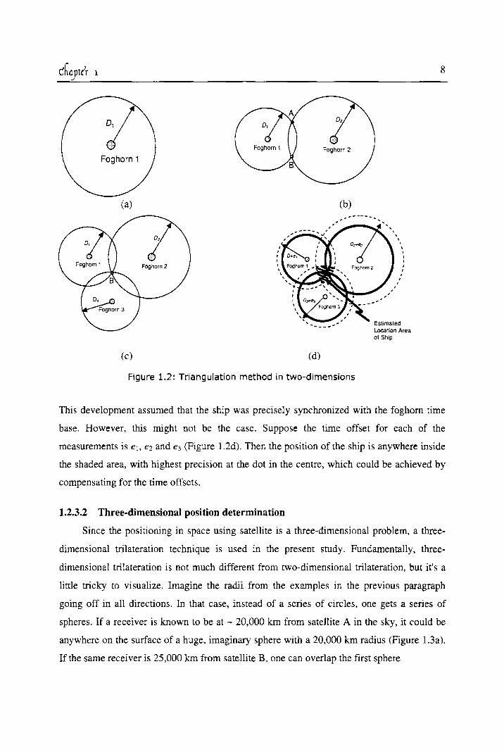
1.2.3.1 Two-dimensional position determination

Consider the case of a ship vessel (receiver) trying to determine its position using a

foghorn (transmitter). The ship should have an accurate clock and the mariner should have

an approximate knowledge of the ship's location. The foghorn whistle is sounded precisely

on the minute mark of the ship clock which is synchronized to foghorn clock. The mariner

records the elapsed time from minute mark to the foghorn whistle being heard. This

propagation time multiplied by speed of sound is the distance from foghorn to the ship.

Based on measurement from one such foghorn, mariner's distance (D]) to foghorn is

calculated. With this the mariner can locate his position anywhere on the circle, as denoted

in Figure I.2a. If mariner simultaneously measured the time range from second foghorn in

same way, assuming transmissions are synchronized to a conunon time base and mariner

knows the transmission times, the ship will be at range D2 from the foghorn 2 (see Figure

l.2b). Therefore, the ship relative to the foghorns is at one of the intersections of the range

circles (point A and B). Since mariner has approximate knowledge of ship's location, the

ambiguity between location A and B can be resolved. If not, then measurement from a third

foghorn is needed (see Figure 1.2c). This method also known as "Triangulation" (or

trilateration), is being used for navigation since time unknown.

(a) (b) , ... ----- ..

.. _----

(c) (d)

Figure 1.2: Triangulation method in two-dimensions

, , I ,

, I ,

I

Estimated Location Area of Ship

8

This development assumed that the ship was precisely synchronized with the foghorn time

base. However, this might not be the case. Suppose the time offset for each of the

measurements is el, e2 and e3 (Figure 1.2d). Then the position of the ship is anywhere inside

the shaded area, with highest precision at the dot in the centre, which could be achieved by

compensating for the time offsets.

1.2.3.2 Three-dimensional position determination

Since the positioning in space using satellite is a three-dimensional problem, a tbree­

dimensional trilateration technique is used in the present study. Fundamentally, tbree­

dimensional trilateration is not much different from two-dimensional trilateration, but it's a

little tricky to visualize. Imagine the radii from the examples in the previous paragraph

going off in an directions. In that case, instead of a series of circles, one gets a series of

spheres. If a receiver is known to be at - 20,000 km from satellite A in the sky, it could be

anywhere on the surface of a huge, imaginary sphere with a 20,000 km radius (Figure l.3a).

If the same receiver is 25,000 km from satellite B, one can overlap the first sphere

(al

(cl

Perfect circle formed from locating two satellites

Possible Locations of GPS Receiver

(dl

Figure 1.3 : Triangulation method in three~dlmenslons

9

with another, larger sphere. The spheres intersect in a perfect circle and the circle of

intersection implies that the GPS receiver lies somewhere in a partial ring on the earth

(Figure l .3b & c). With the help of a third satellite. one gets a third sphere, which intersects

this circ le at two points (Figure 1.3d). The Earth itse lf can act as a fourth sphere -- only one

of the two possible points will actually be on the surface of the planet. so the point in the

space can be eliminated. However. if the receiver is not on the earth surface then it generally

looks for four or more satellites , to improve accuracy and provide precise altitude

information. In order to make this simple calculation, the GPS receiver should know ( I) the

location of at least four satellites above the receiver and (2) the distance between receiver

and each of those satellites. Thus GPS receiver measures the time taken by the transmitted

signal from the different satellites (A, B, and C) to reach the receiver and triangulates for the

10

exact position. While three satellites are essential to detennine latitude and longitude. a

fourth satellite is necessary to determine altitude.

1.3 Different Constellations for Satellite Navigation

Similar to GPS, there are various other satellite based navigation systems which are

either being developed or planned for the global navigation satellite system (GNSS). The

pioneer among them is the Russian GLObal'naya NAvigatsionnaya Sputnikovaya Sistema

(GLONASS), and the European Global Satellite Navigation System (GALILEO).

GLONASS is currently operational and is maintained by Russian ministry of defense.

Similar to the GPS, the GLONASS is a space based navigation system providing global, all

weather access to precise position, velocity and time infonnation to a properly equipped

user. Each GLONASS satellite transmits two carrier frequencies in L-band. The primary

(L1) band ranges from 1.6025 GHz to 1.6155 GHz at an interval of 0.5625 MHz, while

secondary (L2) band from 1.2464 GHz to 1.2565 GHz at an interval of 0.4375 MHz (i.e. 24

channels are available in each band). Each frequency is modulated by 5.11 MHz precision

(P-code) signal or 0.511 MHz CIA signal. Overall, same message code is modulated over

different carrier frequencies for different satellites. As on 2003, out of the intended 24

satellites envisaged only eleven were operational. The twelfth satellite was added in

December 2004 [Ramjee and Ruggieri, 2005]. Hence, this constellation is not operating with

its full capability. However, India has recently agreed to launch a few of their future

satellites [http://www.india.mid.rulsummits/old_07.html] to make the constellation fully

operational.

Moving from ideas and concepts conceived in the 1990s, the European Union (EU)

along with European Space Agency (ESA) intends to operate the GALILEO under

international civil control. This constellation will have 27(+) satellites depending on the

level of international cooperation, the associated ground infrastructure and regional

augmentations. The first phase of launching for GALILEO was accomplished in December

2005 [http://news.bbc.co.ukl2Ihilscience/nature/4555298.stm]. A detail comparison of GPS,

GLONASS and GALILEO systems is presented in Table 1.1. Meanwhile, China has come

out with COMPASS as their regional navigation system. The COMPASS will have a

constellation of 30 non-geostationary satellites and five geo-stationary satellites (GEOs) at

58.750 E, 800 E, 1I0S E, 1400 E, and 1600 E [Hein et al. 2007]. In addition to the global

11

satellite based navigation systems already underway, two regional satnav systems are also

being developed by Japan and India. These systems are Quasi-Zenith Satellite System

(QZSS) of Japan and Indian Radio Navigation Satellite System (IRNSS) of India [Hein et al.

2007]. All these regional systems will be inter-operable and inter-compatible for the

development of a fully operational GNSS.

Table 1.1: A Detail Comparison of the GPS, GLONASS and GALILEO Features

Item GPS GLONASS GALILEO

Operator Department of Ministry of Defence,

EU andESA Defence, USA Russia

Total no of 30 24 27-30

satellites Current status 31 satellites 14 satellites 1 satellites Altitude 20,200 km 19,100 km 23,616 km No. of Orbits 6 3 3 Orbit period 11 hr. 58 min. 11 hr. 15 min. 14 hr. 24 min. Orbit inclination 55° 65° 56° Operating

Ll = 1.575 L1 ;; 1.602-1.615 1.164-1.1215 (E5)

frequencies L2 = 1.227 Lz = 1.246-1.256

1.260-1.300 (~) (GHz) 1.559-1.592 (ETL1-E1)

Clock rate 10 Mbits/sec

i) CIA code 1.023 Mbits/sec 0.511 Mbits/sec 5.11 Mbits/sec 10.23 Mbits/sec 5.11 Mbits/sec 2.046 Mbits/sec

ii) P code 1.023 Mbits/sec

Coordinate WGS-84 ECEF SGS-90 (PZ-90) ECEF ITRFox (IERS)

system GPS time

GLONASS time Time synchronized

synchronized with UTC GST (TAl), UTC (TAl)

with UTC

CIA code: Safety-of-life

Open service. Safety-of-Iife Civilian

applications. Navigation service. Commercial

Service offered application. service. Search and

service. Public regulated rescue. Sub-meter real

P-code: Military time accuracy for

service. Search and Rescue application.

mobile users service.

1.4 Navigation Requirements and Differential GPS (DGPS)

Navigation requirement is the performance of the navigation system, necessary for

operation within a defined airspace. The required navigation performance (RNP) is a part of

a broader concept called "Performance-based Navigation," a method of implementing routes

and flight paths that differs from earlier concepts. This procedure not only has an associated

performance specification which an aircraft must meet before the path is flown, but must

also monitor the achieved performance and provide an alert in the event when this fails to

chayt(f 1 12

meet the specification. RNP equipped aircraft can safely operate routes with less separation

than previously required which is significant because it increases the number of aircraft that

can safely use a particular airspace and therefore accommodate the increasing demand for

air traffic capacity.

1.4.1 Required Navigation Performance (RNP)

The International Civil Aviation Organization (ICAO) developed the RNP approach in

early 1990s and it has become a standard for airspace utilization nowadays. The RNP is a

statement of the navigation perfonnance necessary for operation within a defined airspace.

The main required navigation parameters defined in RTCA [1999] are the following:

(a) Accuracy: It is the degree of confonnance of the estimated or measured position and/or

the velocity of a platfonn at a given time with its true position or velocity. Radio navigation

perfonnance accuracy is usually specified as "Predictable", "Repeatable" and "Relative".

(b) Integrity: It is the ability of the system to provide timely warnings to the user when it

should not be used for navigation purpose. To achieve this, the system has to provide an

alert limit, defined as the maximum error allowable in the user computed position. This alert

limit can be specified in horizontal (HAL) as well as in the vertical (V AL).

(c) Continuity: This is the capability of the total system (including all the elements

necessary to maintain aircraft position within the defined airspace) to perfonn its function

without non-scheduled interruptions during the intended operations.

(d) Availability: This is the percentage of time that a system is performing the required

function under stated conditions. Signal availability is the percentage of time that navigation

signals transmitted from external sources are available to the user.

As an example the required RNP parameters for a GNSS aviation operation are

presented in Table 1.2. This table details about the ICAO requirements from en-route to

Category III (CAT Ill) precision approach operations. All the four main parameters for RNP

along with the alert limit and time-to-alert are provided for each phase of flight operation.

The critical accuracy in vertical direction is not required until the aircraft reaches the

Approach for Vertical Guidance (APV -I and II) operation. The APV s are new classes of less

stringent vertically guided approaches, which have been defined to enable the full utility of

the perfonnance that near-term satellite based augmentation system (SBAS) can provide.

ch")'I'" 1 13

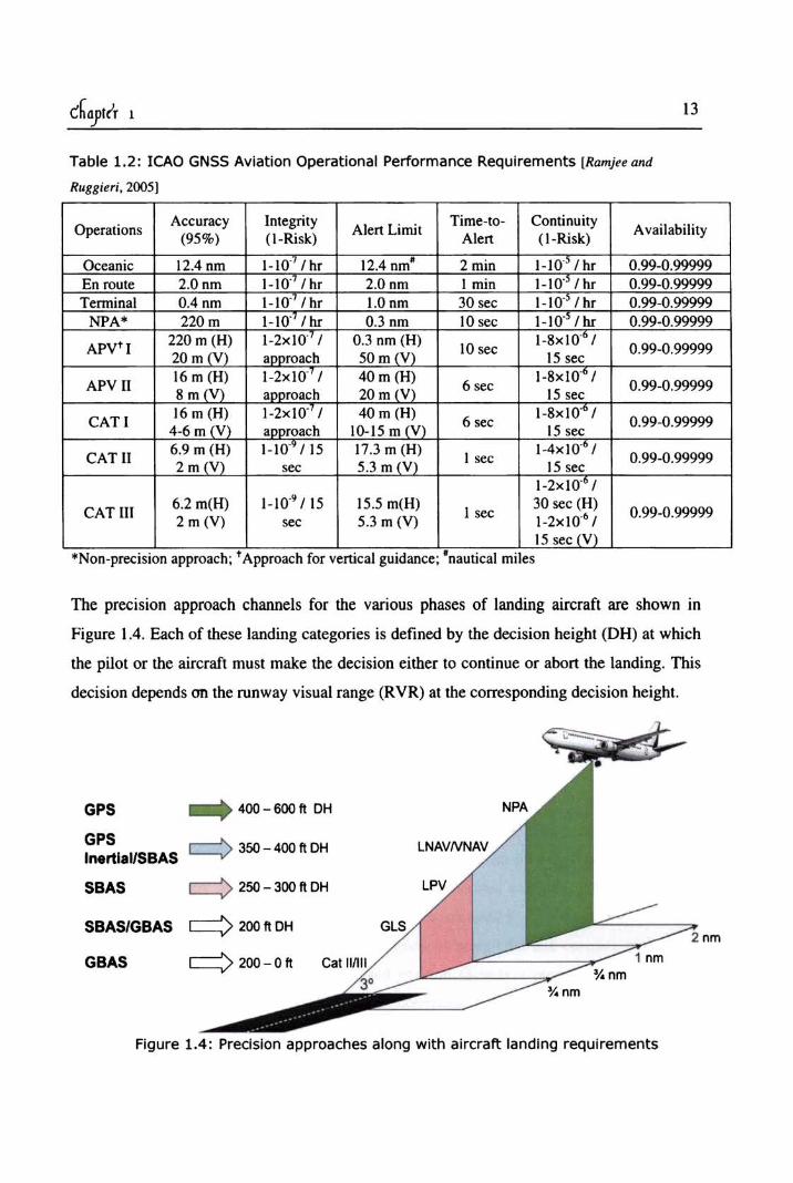
Table 1.2: ICAO GNSS Aviation Operational Performance Requirements (Ramjee and

Ruggieri. 2005 )

Operations Accuracy Integrity

A lert Limit Time-to- Continuity

Availability (95%) (I-Risk) Alert (I-Risk)

Oceanic 12.4 om 1- 10' I hr 12.4 nm' 2min 1-10' I hr 0.99-0.99999 En route 2.0nm 1- 10' I hr 2.0 om I min 1- 1O" /h, 0.99-0.99999 Terminal 0.4 om 1-10' I h, I.Oom 30 sec 1- 10' t hr 0.99-0.99999

NPA· 220 m 1-10' IIrr 0.3 om 10 sec 1-10" /1rr 0.99-0.99999

APVtI 220 m (H) 1-2xlO' I 0.3 om (H) lO sec

1-8x 1O ' 1 0.99-0.99999

20 m (V) approach 50 m (V) 15 sec

APv n 16 m (H) 1-2x lO' I 40 m (H) 6 sec

1-8xlO<1 0.99-0.99999

8 m (V) approach 20 m (V) 15 sec

CAT I 16 m (H) 1-2xlO' I 40 m (H)

6 sec J-8xlO I

0.99-0.99999 4-6 m (V) aooroach 10-15 m (V) 15 sec

CAT 11 6.9 m (H) 1-10' 115 17.3 m (H)

I sec 1-4x IO' I

0.99-0.99999 2 m (V) sec 5.3 m (V) 15 sec 1-2x IO'() I

CAT III 6.2 ro(H) 1-10" 1 15 15.5 m(H)

I sec l O sec (H)

0.99-0.99999 2 m (V) sec 5.l m (V) 1_2xIO·6 /

15 sec (V) . . • *Non-preclslon approach: t Approach for verucal gUidance; nautical miles

The precision approach channels for the various phases of landing aircraft are shown in

Figure 1.4. Each of these landing categories is defined by the decision height (OH) at which

the pilot or the aircraft must make the decision either to continue or abort the landing. This

decision depends on the runway visual range (RVR) at the corresponding decision height.

GPS _ 400-600ft OH

GPS lnertlal/SBAS

c:::::> 350 - 400 ft OH LNAVNNAV

SBAS c:::::> 250 - 300 ft OH lPV

SBAS/GBAS c:::::> 200 ft OH nm

GBAS c:::::> 200 - 0 ft nm

nm

Figure 1.4: Precision approaches along with aircraft landing requirements

14

The three categories of most stringent approach and landings: CAT I, CAT n, and CAT III

are achievable by ground based augmentation system (GBAS). For CAT I the corresponding

values of DH and RVR are 200 ft and >2,400 ft respectively. The same for CAT II (CAT

Ill) are 100 ft (50 ft) and >1200 ft (700 ft).

1.4.2 Differential GPS

A stand-alone GPS has limitations in providing the continuity, availability, integrity

and accuracy to allow for its use as the sole means of navigation for all phases of flight. In

order to meet the operational requirements, augmentation must be applied to basic GPS

signals to eliminate the errors. In augmentation, a supplementary navigation method called

Differential GPS (DGPS) is used to improve significantly the accuracy and integrity of the

stand-alone GPS. The basic categories of augmentation proposed are Satellite~based

augmentation system (SBAS) and Ground-based augmentation system (GBAS).

In the late 1980s, the United States Coast Guard started the development of a Marine

DGPS (MDGPS) system to meet maritime navigation requirements in the United States. In

1989, radio-beacon located on Montauk Point, New York, was modified to broadcast DGPS

corrections in the RTCM SC-I04 (Radio Technical Commission for Maritime Services

Study Committee-l 04) message format. By February 1997, fifty four radiobeacons were

modified to provide DGPS correction for most of the U.S. coastal regions and inland

waterways. In the same year, the coverage was further enhanced throughout the entire

United States. This was named as Nationwide Differential GPS (NDGPS) system. The

MDGPS essentially utilize the code-based Local area DGPS (LADGPS) techniques. The

network for MDGPSINDGPS includes Reference Stations (RS) to monitor GPS and

generate differential corrections. Each RS has two GPS receivers for redundancy along with

collocated Integrity Monitors (IM). Each IM includes another pair of GPS receivers and

radiobeacon receivers to monitor the corrections broadcasted by the same site. The IM

compute their positions and the differential corrections using GPS and compare with their

known (surveyed) positions. If the computed position exceeds a preset tolerance, faulty

satellite is removed from the differential correction calculation after notifying as

"unhealthy" for the user. A frame relay network is used such that two central control

stations, which are manned 24 hours a day, 7 days a week, can monitor the status of all the

sites. The specified accuracy of the MDGPSINDGPS systems is 10 m, 2drms, within

15

coverage areas . Typical accuracies are much better (1 - 3 m). The specified availability is

99.9% for dual coverage areas and 99.7% for areas with single coverage. Later ICAO

developed standards for lbe .wo Iypes of code· based OGPS sySlems (SBAS and GBAS) for

civil aircraft navigation applications.

L4.2.1 S.teltite-based augmentation system (SBAS)

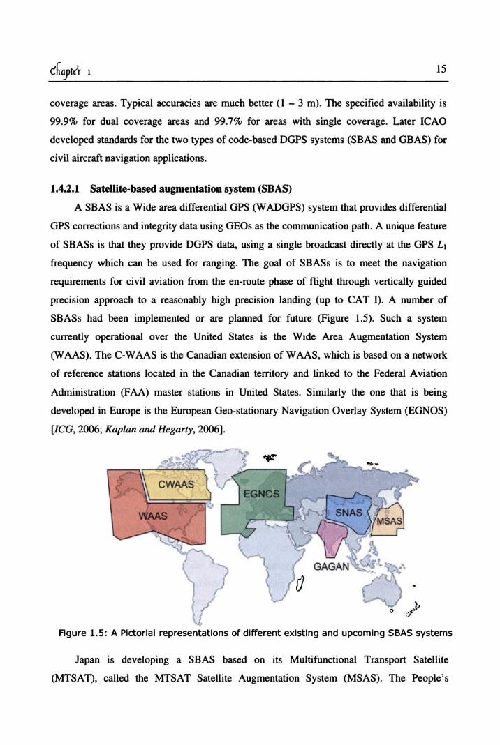
A SBAS is a Wide area differential GPS (W ADGPS) system that provides differential

GPS corrections and integrity data using GEOs as the communication path. A unique feature

of SBASs is that they provide DGPS data, using a single broadcast directly at the GPS LI

frequency which can be used for ranging. The goal of SBASs is to meet the navigation

requirements for civil aviation from the en-route phase of flight through vertically guided

precision approach to a reasonably high precision landing (up to CAT I) . A number of

SBASs had been implemented or are planned for future (Figure 1.5). Such a system

currently operational over the United States is the Wide Area Augmentation System

(WAAS). The C-WAAS is the Canadian ex:tension ofWAAS. which is based on a network

of reference stations located in the Canadian territory and linked to the Federal Aviation

Administration (FAA) master stations in United States. Similarly the one that is being

developed in Europe is the European Geo-stationary Navigation Overlay System (EGNOS)

[ICG, 2006; Kaplan and Hegarty, 2006J.

-- • CWAAS

Figure 1.5: A Pictorial representations of different existing and upcoming S8AS systems

Japan is developing a SBAS based on its Multifunctional Transport Satellite

(MTSAT), called lbe MTSAT Sa.ellj.e Augmen.a.jon SySlem (MSAS). The People's

(hoytir 1 16

Republic of China launched a series of experimental satellites. "Beidou", for mastering the

satellite based navigation technology. The Chinese SBAS strategy is encapsulated in the

Satellite Navigation Augmentation System (SNAS) [Ramjee and Ruggieri, 2005]. India is

also developing its own SBAS called GAGAN (GPS Aided Geo Augmented Navigation)

and it is under the control of the Indian Space Research Organisation and the Airports

authority of India [Kibe. 2003] with planned operational capability by 2009. The other

upcoming regional augmentation systems are the Russian System of Differential Corrections

and Monitoring (SDCM) and the IRNSS of India [leG, 2006; Kaplan and Hegarty, 2006].

In years to come, these regional systems will operate simultaneously and emerge as a Global

Navigation Satellite System to support a broad range of activities in the global navigation

sector. Thus regional augmentation systems will have to play major role in GNSS. The

potential of GNSS will be further enhanced through a focused attention on the coordination

among these regional augmentation systems through maintaining its accuracy. integrity,

reliability and inter-operability everywhere on the globe. Under the proposed framework for

the real-time position determination with high accuracy (- 0.2-0.5 m), the EUPOS

(European Position Determination System) is aimed using DGNSS (Differential GNSS) by

maintaining huge network (- 800 DGNSS reference stations with distance between them

less than 100 km) of ground based stations [Rosenthal, 2007].

All SBAS systems are comprised of four major sub-elements, viz. the monitoring

receivers, central processing facilities, satellite uplink facilities, and one or more

geostationary satellite in orbit. For GAGAN the monitoring receivers are referred to as

Indian Reference Station (INRES), the central processing facilities are known as Indian

Master Control Centre (INMCC) and land uplink facility as Indian Land Up link Station

(INLUS). The GAGAN sub-elements and the functionality provided by them are

summarized in Figure 1.6. As can be seen, the navigation signals received by the user,

transmitted from GPS are also received by monitoring networks or INRES operated by the

SBAS service providers. Each site within the monitoring networks generally includes a

number of GNSS receivers (for redundancy) that provide Ll CIA code and L2 P(Y) code

pseudorange and carrier-phase data to the central processing facilities or INMCC. At

INMCC the data from the entire network are processed to develop estimates of each GPS

satellite's true position, associated clock error, corrections based on the differences between

the networks estimates of these parameters and the values in the broadcast GPS navigation

17

data, and estimate of Ionospheric and Tropospheric delay error across the service area.

These estimates and integrity infonnation are then forwarded to the satellite up-link facilities

GPS l1~

!\Aa 1;'IIItES (RIM )

C DAND 0 LJ ,LS

o GEO • P$l1 / L2

i All INRES (RIM)

INLUS

Figure 1.6: The GAGAN sub-elements and its functionality

(INLUS). From INLUS the signal is continuously transmitted to a geostationary satellite via

C-band, which is further transmitted to the user at L! and Ls frequencies . The timing of the

signal is done in a very precise manner such that the signal appears as though it was

generated on board the satellite as a GPS ranging signal.

1.4.2.2 Ground-based augmentation system (GRAS)

In a Ground-based augmentation system, SPS is augmented with a ground reference

station to improve the performance of the navigation services in a local area. The only

operational GBAS is the Large Area Augmentation System (LAAS) of the U.S. Federal

Aviation Administration. This can support all phases of flight within its coverage area,

including precision approach, landing. departure, and surface movement. In GB AS system.

Pseudolites (PL) or integrity beacons (low· power ground based transmitters) are configured

to emit GPS·like signals for improving accuracy. integrity. and availability of GPS

[Parkinson and Spliker, 1996; Van Dierendonck. 1990; Elrod and Van Dierendonck. 1993;

EJrod et al., 1994}. The improvement in accuracy can thus be obtained by enhancing the

local geometry, measured according to a lower Vertical Dilution of Precision (VDOP) which

chayttT 1 18

is very crucial for aircraft precision approach and landing. The accuracy and integrity is

further improved by using PL integral data link to support DGPS operations and integrity

warning broadcast. Furthennore, the PL provides additional ranging source to augment the

GPS constellation for enhancing its availability. The PL operates at the Ll frequency and is

modulated with an unused PRN code, in order not to be confused with a satellite signal. A

second GPS antenna mounted on the aircraft is used to acquire the PL signal. The presence

of two PLs which are generally placed within several miles of a runaway threshold along the

nominal approach path reduces the requirement of visible satellites for DGPS operations to

four, and centimeter-Ievel position accuracy can be achieved [Schuchman et al., 1989; Elrod

and Van Dierendonck, 1993; Cohen et al., 1994].

1.5 Errors in GPS Signal

Accuracy of the position detennined by GPS is ultimately expressed as the product of

a geometry factor and a pseudorange error factor. Error in GPS solution is estimated by the

fonnula: (error in GPS solution) = (geometry factor) x (pseudorange error factor). The

pseudorange is the actually measured range which includes the errors that limit the GPS

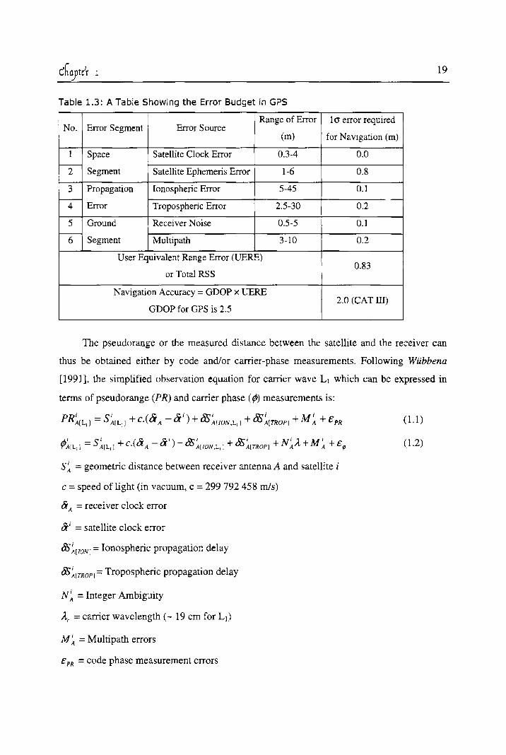
stand alone system to achieve the RNP up to the stringent CAT III condition. A detailed list

of different sources of error in GPS ranging along with the range of these errors as well as

the contribution from each error required to bring it down for navigation purpose (at CAT III

level) is presented in Table 1.3. With appropriate assumptions, the pseudorange error factor

is the satellite User Equivalent Range Error (UERB), which comprises of the components

from all the three segments of the GPS system. The Space segment comprises of the satellite

clock error and broadcasted ephemeris error. The ground segment has error contribution due

to receiver noise and the multipath effect. The errors introduced by the propagation of GPS

signal through the intervening atmosphere are the Ionospheric error and the Tropospheric

(neutral atmospheric) error. All these errors are combined by root-sum-squared (RSS) to

yield the UERE. The RSS addition for UERB is justified under the assumption that the

errors can be treated as independent random such that the 1-sigma total error is the RSS of

the individual I-sigma values. The geometry factor, which expresses the composite effect of

the relative satellite/user geometry on the GPS solution error, is generally known as the

Geometric Dilution of Precision (GDOP). The GDOP value for a GPS system is 2.5, thus

UERE value of 0.83 can achieve a CAT III level of position accuracy.

19

Table 1.3: A Table Showing the Error Budget in GPS

No. Error Segment Error Source Range of Error 1 er error required

(m) for Navigation (m)

I Space Satellite Clock Error 0.3-4 0.0 -

2 Segment Satellite Ephemeris Error 1-6 0.8

3 Propagation Ionospheric Error 5-45 0.1

'4 Error Tropospheric Error 2.5-30 0.2 -

5 Ground Recei ver Noise 0.5-5 0.1 c---

6 Segment Multipath 3-10 0.2

User Equivalent Range Error (UERE) 0.83

or Total RSS

Navigation Accuracy = GDOP x UERE 2.0 (CAT Ill)

GDOP for GPS is 2.5

The pseudorange or the measured distance between the satellite and the receiver can

thus be obtained either by code and/or carrier-phase measurements. Following Wubbena

[1991], the simplified observation equation for carrier wave Ll which can be expressed in

terms of pseudorange (PR) and carrier phase (,) measurements is:

s~ = geometric distance between receiver antenna A and satellite i

c = speed of light (in vacuum, c = 299792458 m/s)

£0 A = receiver clock error

£oi = satellite clock error

&'~[lONI = Ionospheric propagation delay

&' ~[TROPl = Tropospheric propagation delay

N~ = Integer Ambiguity

Ac = carrier wavelength (- 19 cm for L 1)

M ~ = Multipath errors

E PR = code phase measurement errors

(1.1)

(1.2)

20

EIP ::: carner phase measurement errors

Understanding of the significance of these errors is important in applications that require

very high accuracy. Each of these errors is briefly discussed in the following subsections.

1.5.1 Satellite Clock Error

The atomic clocks in GPS satellites, although highly accurate, are not perfect. The drift

of these clocks from GPS system time, results in pseudorange error. The GPS time is a

composite time scale derived from the times kept by clock at GPS monitoring stations along

with the onboard satellite clock, which is used as the reference time. The GPS time which is

set at OOh on 6th Jan 1980 and presently ahead of UTC by 14 seconds has not been perturbed

by leap seconds. The atomic clocks stability is about 1 to 2 parts in 1013 over a period of one

day. This means the satellite clock error is about 0.864 to 17.28 ns, which introduces

arround a 0.3-4 m error in ranging [Kaplan and Hegarty, 2006]. The Master control station

determines the clock errors of each satellite and transmits clock correction parameters to the

satellites for re-broadcasting to the user along with the navigation message.

1.5.2 Ephemeris Error

Ephemerides of all satellites are computed and up linked to the satellites along with

other navigation data for re-broadcasting to the user. These ephemerides (in satellite

navigation messages) are predicted from previous GPS observations at the ground control

station. The satellite ephemeris error is the difference between the actual position and

velocity of a satellite and those predicted by the broadcast ephemeris model. The residual

satellite position error is in the range 1-6 m [Warren and Raquet, 2002].

1.5.3 Multipath

This refers to the phenomenon of a signal reaching the receiver antenna through two or

more paths. Typically an antenna receives the direct signal along with one or more of its

reflections from structures in the vicinity and also from ground. The reflected signal is

delayed and usually weak compared to the direct signal. The multipath though affects the

code as well as the carrier phase measurements; the magnitude of this error differs

significantly. The error due to multipath effect is usually within 3-10 m [Kaplan and

Hegarty, 2006]. A primary remedy for avoiding multipath is to place the antenna away from

21

reflectors, which may not be practical always. The affect of mUltipath can then be reduced

by suitably designing the antenna consequently lowering the contribution from side lobes. In

benign environments, such as open field, placing an antenna closer to the ground can

decrease observed multipath errors because when the antenna is near to ground the signals

experiences shorter excess path delays that tend to produce smaller multipath errors. Choke

ring antennas are the special kind of antp.nnas which are successful in mitigating the

multipath arrivals from the ground or low-elevation scatterers.

1.5.4 Receiver Noise

The code and carrier phase measurements are affected by random noise, which is

usually referred to as receiver noise. This includes the noise introduced by antenna,

amplifiers cables and the receiver. The receiver noise varies with the signal strength, which

in turn varies with the satellite elevation angle. The dominant source of error in pseudorange

measurements is the thermal noise jitter and the effects of interference. The CIA code

composite receiver noise and resolution error contribution are slightly larger than that for

P(Y) code because the former has a smaller rms bandwidth than the latter.

1.5.5 GPS Signal Propagation Errors

The Microwaves as they propagate through the atmosphere undergo scattering,

attenuation and refraction. As the GPS signal lies in the L-band of the Microwave frequency

domain, the contribution of signal delay due to scattering and attenuation is negligible. So

the delay in the GPS signal when it traverses through the atmosphere is mainly due to the

refractive nature of the intervening atmosphere. However, the L-band is aptly chosen

frequency band as the refractive effect of ionosphere is moderate, and that of neutral

atmosphere is least, at these frequencies. For GPS application, the atmospheric regions of

interest for error budget are mainly the neutral atmosphere and ionosphere. The effect of

neutral atmosphere ranges from the surface of the earth up to approximately 100 km in

altitude, where as that of the ionosphere ranges from 75 km and more. The delay caused by

the ionized region of the atmosphere is called the Ionospheric delay and that by the neutral

atmosphere is Tropospheric delay (as 98% of the neutral atmosphere is contained in the

troposphere ).

22

1.5.5.1 Microwave propagation in the atmosphere

The earth's atmosphere is a heterogeneous medium with significant variations of its

physical parameters such as temperature, pressure and humidity, etc, prominently in vertical

direction. When microwave propagates through such a medium, it introduces a small

retardation as well as bending of the ray path. The velocity (v) of an electromagnetic wave

in a medium having a refrl'ctive index n, is written as v = cln where c is its velocity in

vacuum. For most of the physical media, n > 1, which implies that the speed of the

propagating electromagnetic (EM) wave is less than that in vacuum. The value of n is

characterized by permeability (1) and dielectric constant (E) of the medium. The expression

for v can then be written as v = cl ~ j.iE . If )lo and Eo are the permeability and dielectric

constant of free space, respectively, then c = ~ 110 Eo' For a refractive medium (E > Eo), the

wave propagates with a velocity which is less than that in free space (i.e. v < c).

In general, the index of refraction is a complex quantity with its real component

representing the non-absorbing part of the medium and the imaginary part representing the

attenuation of electromagnetic waves by the medium. In microwave domain the refractive

index of air is a function of temperature, pressure and humidity. As all these three

parameters decrease with increase in altitude, n also decreases with altitude. At standard

temperature and pressure, n "" 1.0003 [Pett),. 2004]. It approaches unity with increasing

altitude. As a result, the ray path bends towards the earth surface due to refraction. The

decrease in velocity and bending of ray-path introduces an error in the measured range

which is taken as the product of the velocity of the wave in free space and time taken by the

wave to trace the in-between region. A typical i11ustration of the propagation of radio waves

in the atmosphere from a transmitter in the sate11ite to the observer on the earth's surface is

presented in Figure 1.7. As virtual1y there is no atmosphere above the ionosphere, the ray

does not undergo any pronounced deviation in this region. Neglecting the horizontal

variability. the atmosphere can be divided into a number of concentric layers each of

thickness ds, with ni as the refractive index for each layer. The time taken by a ray to travel

from a distant satellite to receiver is equal to ~t = l/e Inds and the apparent range R = e x

~t. The error in the estimated range (~R) due to extra time (~t) incurred by the refraction

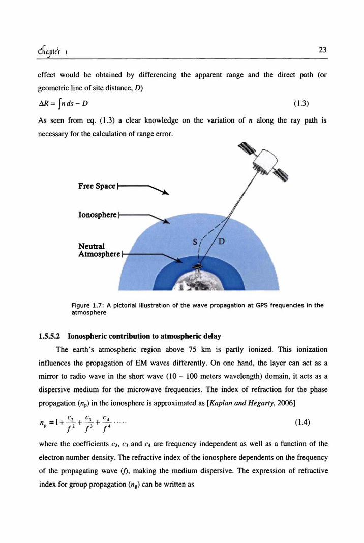
23

effect would be obtained by differencing the apparent range and the direct path (or

geometric line of site distance, D)

!1R. = Inds - D ( 1.3)

As seen from eq. (1.3) a clear knowledge on the variation of n along the ray path is

necessary for the calculation of range error.

Free Space t-I ---'-:....

Ionosphere 1----... ........... ------;4, Neutral

Figure 1.7: A pictorial illustration of the wave propagation at GPS frequencies In the atmosphere

1.5.5.2 Ionospheric contribution to atmospheric delay

The earth's atmospheric region above 75 km is partly ionized. This ionization

influences the propagation of EM waves differently. On one hand, the layer can act as a

mirror to radio wave in the short wave (10 - lOO meters wavelength) domain, it acts as a

dispersive medium for the microwave frequencies. The index of refraction for the phase

propagation (np) in the ionosphere is approximated as [Kaplan and Hegarty, 2006]

Cl C] c~ n = 1+-+-· +_ ..... , f' f' f'

(1.4)

where the coefficients q, Cl and C4 are frequency independent as well as a function of the

electron number density. The refractive index of the ionosphere dependents on the frequency

of the propagating wave (j). making the medium dispersive. The expression of refractive

index for group propagation (ng) can be written as

dn ng =np + f--P

df

Substituting eq. (1.4) in eq. (1.5) ng can be written as

c2 2c3 3c4 n =1------····· g f2 f3 f4

Neglecting the higher order terms one can write

24

(1.5)

(1.6)

(1.7)

The coefficient c2 is estimated as c2 = -40.3 ne HZ2, where ne is the electron number

density. Then eq. (L 7) can be rewritten as

-1- 40.3n. np - 2

f -1 40.3ne n. - + 0

C f-

The phase and group velocities are then estimated as:

c v =---­p 1- _40_.3_n_e

f2

c v =----g 40.3ne

1+ 2

f

(1.8)

(1.9)

In case of microwave propagating through the ionosphere, it experiences a group retardation

and phase advance. a phenomenon referred to as ionospheric divergence. The refractive

index of the ionosphere varies inversely with the square of radio frequency and so

ionospheric refraction is more significant at lower frequencies (below S-band) [Kaplan and

Hegarty. 2006]. The range error associated with the microwave propagation through the

ionosphere is

(1.10)

where f ne dl is the electron density along the path length. referred to as the total electron

count (TEC). Since the TEC is generally referenced to the vertical direction through the

ionosphere, for other elevation angles the M iono is to be multiplied by an obliquity factor

(OF) or mapping function given as

(1.11)

25

where hI is the height of maximum electron density (- 350 km), re is the radius of earth and

cA is the elevation angle. With addition of the OF the path delay expression becomes

=-0 40.3 TEC F 12 (1.12)

This dispersive behavior of ionosphere to microwave propagation is used for estimating the

ionospheric delay by making the '1leasurements at two frequencies say Lr and L2•

Differencing the pseudorange measurements made on both Lt and L2 frequencies enables

the estimation of delays in both the Lt and L2. Thus to account for the ionospheric delay one

uses the following expressions for Ll and L2

(l.13a)

(1.13b)

where PLt

and PL, are the pseudorange observations at L\ and L2• For various civilian

applications including navigation, single-frequency receivers are used. Then it is obvious

that one cannot use eq. (1.13) or the dual frequency technique to estimate the ionospheric

delay. Consequently, models of the ionosphere are to be employed to correct for the

ionospheric delay. One important example of such a model is the Klobuchar model, which

removes (on average) about 50% of the ionospheric delay at mid-latitudes through a set of

coefficients included in the GPS navigation message [Kaplan and Hegarty, 2006]. Another

method of removing the ionospheric delay in a single frequency receiver for navigation is by

providing near-real time TEC values from the reference stations (consisting of minimum

three dual frequency receivers). These dual frequency receivers estimate the TEC for each

reference station in-and-around the user and provide the TEC infonnation to the user

through broadcasting via a geostationary (communication) satellite link. To achieve this

more efficiently, one has to have a dense network of reference stations.

Thus to summarize, the ionosphere is characterized by a large concentration of free

electrons that cause a variation of the channel refractive index and, consequently, of the

wave propagation velocity in the medium. In particular, the ionosphere effects on the GPS

signals mainly result in 1) a combination of group delay and carrier phase advance, which

varies with the paths and electron density encountered by the signal in crossing the

26

ionosphere, and 2) scintillation, which can bring the signal amplitude and phase to fluctuate

rapidly at certain latitudes and even cause loss of lock. Other effects related to the

ionosphere, such as Faraday's rotation and ray bending that changes the arrival angle, are

not significant for the GPS frequencies. In the GPS frequency bands, the Ionospheric path

delay in zenith direction might vary from 2-50 ns, in a diurnal fashion that is quite variable

and unpredictable from day-to-day. At lower elevation angles, the delay might inrrease up to

three times the value at the zenith. This implies that the Ionospheric error can contribute in

the range of 5-45 m [Ramjee and Ruggieri, 2005]. The ionosphere being a dispersive

medium (frequency dependent), dual (or multi) frequency observations helps to reduce this

delay. Note that as the present study is focused only on the effect of neutral atmosphere in

microwave ranging, the refraction effects in the ionosphere will not be considered in

subsequent discussions.

1.5.5.3 Contribution of neutral atmosphere to atmospheric delay

Most of the neutral constituents in the atmosphere reside in the lower part of the

earth's atmosphere. The neutral density decreases exponential1y with increase in altitude

following the hydrostatic eqUilibrium. Though the concentration of the major neutral

constituents (N2, 02, Ar, etc) decreases with altitude almost all the water vapor and bulk of

the dry gases are found in the troposphere which ranges from sea level (",0 m) to - 12 - 16

km. In this region, the temperature in general decreases almost linearly with increase in

altitude with a fixed lapse rate. The altitude extent of the troposphere varies with latitude.

The region separating the troposphere from the atmosphere above it is known as tropopause

where the temperature gradient is very small and approaches close to zero. The region above

the tropopause, where the atmospheric temperature starts increasing with altitude, is referred

to as stratosphere. In addition to the major constituents, the neutral atmosphere also contains

significant amount of trace constituents like CO2, 0 3 and water vapor. All these gases in the

atmosphere, except water vapor are non-polar molecules, while water vapor is polar in

nature. A polar molecule will have a pennanent electric dipole moment and it aligns itself to

the applied electromagnetic field, while a non-polar molecule do not have a pennanent

electric dipole moment and this will be induced when an external electromagnetic field is

applied. While the non-polar gas molecules are well mixed in the atmosphere and obey the

hydrostatic equations, water vapor is not well mixed.

27

As the refractive index of air is greater than unity, the wave propagation through this

medium undergoes group retardation. In addition to that the ray-path is curved because of

the refractive bending. The group retardation and bending of the ray affect the net apparent

path length traveled by the wave and can be estimated as the integral of the refractive index

(n) profile (eq. 1.3) along the curved path. If '5' is the curved path and 'D' is the direct path

lengtl} then the extra path length estimated through ranging is t\Rtropo = Js n.ds - D = Js (n­

l).ds + [5-D]. Considering the wave propagation in vertical, as there is no refractive bending

'5' will be identically equal to 'D'. Then the extra path encountered in the zenith direction,

usually referred to as zenith tropospheric delay (ZTD) is r (n -l).ds , where the integral is

taken for the entire neutral atmosphere. The equation can be written in terms of the

refractivity (N) of the air as ZTD = 10-6 X IN ds = 10.6

X [INo ds + INw ds] where No and Nw

represents the hydrostatic (dry) and non-hydrostatic (wet) component of refractivity,

respectively. The net tropospheric delay in the zenith direction thus has two parts, one

governed by the non-polar gases (hydrostatic), which is usually referred to as zenith

hydrostatic delay (ZHD) and the other contributed by water vapor which is referred to as the

zenith wet delay (ZWD). While the hydrostatic (dry) component constitutes about 90% of

the total delay, the non-hydrostatic (wet) part constitutes the remaining 10%. More details

on tropospheric delay due to refraction and its estimation are presented in Chapter 2.

The refraction of the Microwaves at GPS frequencies as it passes through the entire

neutral atmosphere is referred to as tropospheric delay [Misra and Enge, 2001; Barry and

Chorley, 1998]. The GPS signals when it traverses through the troposphere it induces delay

effects in the order of 2-30 m [Ramjee and Ruggieri, 2005]. These effects depend on the

density of atmospheric gases as well as the zenith angle at which the ray propagates.

Complete information on different atmospheric parameters like pressure (P), temperature (T)

and water vapor partial pressure (e) is essential to estimate this delay. At GPS frequencies,

the delay caused by troposphere is one order in magnitude less than that caused by the

ionosphere. But this delay is almost the same for both LJ and L2 frequencies. Since it is not

frequency dependent (non-dispersive), this effect cannot be eliminated using dual (or multi)

frequency measurements. However, this can only be accounted for through modeling. The

existing global models are successful in predicting the dry part of the delay with an accuracy

of approximately 1 cm and the wet part with - 5 cm [Kaplan and Hegarty, 2006].

(haYfer 1 28

1.6 A Review of Different Models for Estimating Tropospheric Delay

Different empirical meteorological models are developed for the estimation of the

ZHD and ZWD on a global basis. Saastamoinen [1972] evolved a simple relation between

ZHD and surface pressure (Ps) taking into account the variation due to gravity and height

for different latitudes. The claimed accuracy of the Saastamoinen model is within 0.4 km for

all the latitudes and seasons. Later on Davis et af. [1985] and Elgered et al. [1991] proposed

similar expressions for ZHD with a slightly different value for the coefficients. All these

models are developed under the assumption that the dry atmosphere is in hydrostatic

equilibrium and follows the equation of state. However, since water vapor does not follow

the hydrostatic conditions and can remain heterogeneously distributed in the atmosphere,

similar models for ZWD were not attempted until Ifadis [1986] and Mendes and LangZey

[1998] developed simple empirical relation connecting ZWD with Ps, surface temperature

(Ts) and surface water vapor partial pressure (es). A slightly different model for ZHD and

ZWD was arrived by Hopfield [1971], based on a different refractivity model. A brief

outline of these models is presented in the following subsections.

1.6.1 Linear Models for ZHD and ZWD

Saastamoinen [1972] showed that although the refractivity at any point in a dry

atmosphere depends on pressure and temperature, the height integral of this dry refractivity

profile would be a simple linear function of surface pressure. The main assumption in this

model is that the dry atmosphere is in hydrostatic equilibrium and the equation of state

dP =- g(h)·p(h)·dH g (1.14)

is true. Here the acceleration due to gravity (g) is a function of height (h), p is the density of

the air and Hg is the geopotential height (in m) or the vertical coordinates with reference to

earth's Mean Sea Level (MSL). If g is assumed to be a constant with a weighted mean value

gm then eq. (1.14) can be written as

1 dP p=-_.-gm dH g

(1.15)

This equation along with the ideal gas law (P = pRdT) can be used to estimate the ND value

as

N = [k P]=k -R .p=-k -R ._1 __ dP D IT 1 d 1 ,I dH

gm g

(1.16)

chayte'r 1 29

where k\ = 77.6 KJhPa, is hydrostatic refractivity constant [Bevis et al., 1992], P is pressure

(hPa), and Rd is gas constant of dry air (J kg- l Kl). Then the ZHD can be written as

( 1.17)

where R* is the universal gas constant (=8314.3 j kmorl K i), Md is the molecular weight of

dry air (= 28.9644 kg/kmol) and the gm is defined as

00

jP(h). g(h)· dh hs gm = -'--00----- ( 1.18)

jP(h)'dh hs

and can be interpreted as the gravity at the centroid of the atmospheric column

[Saastamoinen, 1972]. The value of gm depends on latitude through the relation [Davis et al.,

1985]

gm = 9.8062' (1- 0.00265· cos 2cp- 0.00031- he) (1.19)

where cp is the ellipsoidal latitude and the he is the height of the center of the atmospheric

column above the ellipsoid (in km), which is linearly modeled by Saastarnoinen as

he = 7.3 + 0.9 X h; where h is the height of the antenna site above the ellipsoid (km).

Substituting this in eg. (1.19) the expression for gm can be written as

gm = 9.784· (1- 0.00266· cos 2cp- 0.00028· h)

Then from eg. (1.17)

ZHD = 0.0022767· Ps 1- 0.00266· cos 2cp - 0.00028· h

(1.20)

( 1.21)

This model is very popular due to its simplicity. The rms error budget using Saastamoinen

model [Elgered et al., 1991] shows that the error in the refractivity constant contributes to

about 2.4 mm in ZHD. The uncertainty in gm has only a marginal influence of 0.2 mm and

the uncertainty of the universal gas constant and the variability of the dry mean molar mass

contributes approximately 0.1 mm in the estimation of ZHD. Thus, in this model along with

surface pressure measurements the height of the station and its latitude are used for the

computation of the gravity correction. Though a similar model was not tried for ZWD in the

30

earlier attempts mainly due to the heterogeneity of the distribution of water vapor in the

atmosphere, later Chao [1972], Berman [1976], and Saastamoinen [1972] tried to develop

models for the wet component but with obsolete value of refractivity constants. All these

models were either station or season specific and had biases of up to 10-20 % depending on

the site.

Ifadis [1986] proposed a model for the zenith wet delay as a function of Ps, Ts and es

in the following form.

ZWD = 0.554 .10-2 - 0.88 .10-4

• (Ps -1000)

e +0.272.10-4 ·e~ +2.771---.l...

, Ts

Mendes and Langley L 1998] derived a linear relation for ZWD in the form

ZWD = 0.122 +0.00943· es

(1.22)

(1.23 )

relating zenith wet delay and partial water vapor pressure at the surface using data from

about 50 stations, most of which are located in USA and Canada.

Though meteorological parameters at surface are correlated reasonably well with the

range error, these surface models are not efficient enough to account for the complete

integral effect of atmospheric refraction in vertical direction [Bock and Doeiflinger, 2000].

In case, if the required range is from a particular altitude in the atmosphere, the refraction

effect for the altitude above, only need to be accounted for. In this context, Hopfield [1971]

tried to develop a model accounting for the variation of atmospheric refractivity with

altitude through an analytical function.

1.6.2 Hopfield Model for ZHD and ZWD

Hopfield [19691 developed an analytical model for the altitude profile of refractive

index based on surface refractivity (Ns) and a term called the "characteristic height" which is

different for the hydrostatic and non-hydrostatic component of refractivity. These

characteristic heights are defined as the altitude above which the atmospheric refraction

effect is negligible. This implies that the values of ND and Nw become negligible above the

respective characteristic heights. Once the mean annual pattern of characteristic height is

modeled for a station, it is possible to estimate the range error directly from surface

refractivity. These analytical relations are arrived based on following approach.

31

The equation for hydrostatic equilibrium (eq. 1.14) that follows from the ideal gas laws

of Boyle-Mariotte and Gay-Lussac can be expressed in differential form by expressing the

density as p=_P_ in the form R,-T

P dP g dP=-g ·--·dh (::} -=---·dh

Rd -T P Rd·T (1.24)

The altitude profile of the temperature in the troposphere can be approximated to be linear

with a constant temperature lapse rate (/1) in the form T = Ts + f3 . h, where Ts is

temperature at the surface (or antenna height), h is the height above MSL and T is a function

of altitude. Substituting this in eq. (1.24) the differential equation takes the form

dP == g ·dh

R . (T + (3- h) d S

( 1.25) P

Integrating this equation for altitude region 0 to h where the atmospheric pressure decreases

from Ps to P

( 1.26)

Now, let us recall the hydrostatic refractivity formula:

(1.27)

The total density of air, p is the sum of density of dry air (Pd) and that of water vapor (Pw)

given as

( 1.28)

where Mw is the molecular weight of water (=18.016 kg/kmol). If one considers that Pd» e

and Pd' Md» e .Mw then it is acceptable to approximate that Md"" Mw. Then the p becomes

Substituting this in eg. (1.27) the expression for ND becomes

N = k . R . P = k . R . _P- = k . P D ! dId R.T I T

d

Substituting for P and T

g

N =k·-=k· .p. P 1 (Ts +j3.h»)-R,;.P

D ] T ] Ts + j3 . h S Ts

which can be further simplified to

g

N =k . P =k . Ps .( Ts ).(T5 +f3' h)]-R"'/3 o 1 TIT T +f3·h T

S 5 5

- (Ts +f3'h)]-(!+~~p) _ (j3.h]TJ -Nso ' -N so ' 1+--

Ts Ts

32

(1.29)

( 1.30)

( 1.31)

(1.32)

p where N SD = k] . _S . For a default temperature lapse rate of j3 = -6.81 Klkm and a mean

Ts

gravity acceleration of g = 9.806 m/s2 the exponent becomes 11 = 4.02 ::::: 4 that is adopted for

the Hopfield two-quartic model. Another modification is made by substitution of

j3 =-----

1 1 I -·T -h j3 s 00

I h --·T 00 j3 S

0.33) -----=

where Ts is the surface temperature in QC; hO~ is the characteristic height of the dry

atmosphere for temperature of OQC (in km) and hD is the characteristic height of the dry

atmosphere (in km). The variation of ho (in km) with Ts (in QC) is modeled from global

radiosonde data as

hD = 40.136+0.14872xTs (1.34 )

As stated above employing a value of 4 for 11, ND is simplified as

N =N '(1_~)4 D so h

o (1.35)

eg. (1.32) can then be integrated analytically to yield ZHD as

33

hlr[ h )4 h ZHD=10-6 ·N· 1-- dh=1O·6·N .-.!2... so h SD 5

o D

(1.36)

It is clear that a number of approximations lead to this simple formula. Apart from the fact

that the air is treated as an ideal gas which is not too critical, the assumption of a constant

temperature lapse rate is one important approximation that should be stressed as well as the

fact that the gravity is not modeled in terms of its dependence on the height, as was done for

Saastamoinen model.

Hopfield [1969] assumed that the non-hydrostatic component of N also follows the

similar relationship but with a different value for the characteristic height. Thus in analogous

to eq. (1.35) an expression for the non-hydrostatic component can be written as

( 1.37)

where hw is the wet characteristic height. The wet delay then can be written as

hr[' h )4 h ZWD = 10.6 . N . 1 - - dh = 10.6

• N . ~ sw h .sw 5

o w (1.38)

Mendes and Langley [1998] found a relation between the surface temperature (in QC) and hw

(in km) of the form

hw =7.508+0.002421.exp(~) 22.90

0.39)

The estimation of the ZWD based on Hopfield method needs only the information about es

and Ts [Hopfield. 1969J. As hw is not well correlated with Ts. there will be some uncertainty

in the estimation of ZWD using this model. Analysis shows that a 10% error in the value of

hw can introduce an error of < 1 % in the estimated value of ZTD and hence can be neglected

for application purpose.

Even though all these empirical models are considered as global, most of these are

experimentally derived using the available radiosonde data from European and North

American continents [Satirapod and Chalermwattanachai, 2005]. The accuracy of these

empirical models has been assessed by comparing model output with true values estimated

by ray-tracing the atmospheric profiles. It has been shown that ZHD models are typically

accurate up to 2-3 mm at mid-latitudes [lanes et al., 1991], and estimates of ZWD from

surface meteorological data exhibit typical errors of up to 3-5 cm [Askne and Nordius, 1987;

chaytc'r 1 34

lanes et al., 1991; Elgered, 1992] and up to 5-8 cm during the passage of weather fronts

[Elgered, 1993; lchikawa, 1995].

1.7 Projecting the Zenith Tropospheric Delay to Slant Direction

The tropospheric delay is shortest in zenith direction and increases with zenith angle.

In many cases for the use of GPS in navigation and meteorology it becomes necessary to use

the data from higher zenith angle mainly because of the fact that usage of a high zenith angle

expands the observation geometry in navigation application while increases the amount of

data availability in meteorological applications. Many investigators [Ware et al., 1997;

Flares et al., 2000; Braun et al., 2001; Mac Danald and Xie, 2000] have elaborately studied

the effect of very high zenith angles in GPS slant observations in relation to meteorological

applications. Studies have shown that though the tropospheric delay is - 2 m in the zenith

direction, it increases to over - 20 m at high zenith angle [Ramjee and Ruggieri, 2005;

Dodson et al., 1999a], thus exceeds the criteria set for optimum positioning for civil

navigation [Kaplan and Hegarty, 2006]. In general the tropospheric delay at a given zenith

angle (x), referred to as slant total delay (M), which is related to zenith delay as

M = ZHD x MFh(x) + ZWD x MFw(x) (1.40)

This projection of zenith path delay into a slant direction is performed by application of a

mapping function (MF) or obliquity factor. The first part in eq. (1.40) is the hydrostatic

component of slant delay (SHD) and the second part represents the non-hydrostatic

component of slant delay (SWD). Thus the mapping functions are defined as

MF ( ) = SHD h X ZHD

MF ( ) _ SWD w X - ZWD

(1.41a)

(1.41b)

Tracing the ray-path through the refractivity profiles (derived from the radiosonde data)

provides an estimate of mapping function [Rocken et al. 2001], which is also know as direct

mapping function (or true value of MF). Simplest analytical function for MF is the cosecant

function. The upper limit of use of this function for many applications is - 60° (zenith

angle). In higher zenith angles, Marini [1972] showed that for a spherically symmetric

atmosphere the MF can be approximated by a continued fraction, which was later on

modified by Herring [1992], Niell [1996] etc. Niell [2000] also proposed an isobaric

35

hydrostatic mapping function (IMF) which uses only one meteorological input parameter

(the height of the 200 hPa isobar). The most commonly used MF among the analysts is Niell

mapping function (NMF) [Ni ell, 1996] the coefficients for which are determined from site

coordinates and the day of the year using a look-up table. Recently, a Global Mapping

Function (GMF), based on data from the global ECMWF numerical weather model was

developed by Boehm et al. [2006a]. The coefficients of GMF were obtained from the

expansion of the Vienna Mapping Function (VMF1) parameters [Boehm et al. 2006b] into

spherical harmonics on a global scale. In the following section three of these global MFs are

discussed in detail.

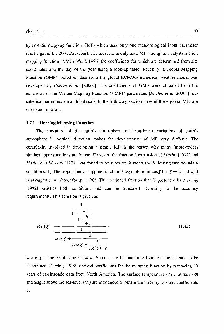
1.7.1 Herring Mapping Function

The curvature of the earth's atmosphere and non-linear variations of earth's

atmosphere in vertical direction makes the development of MF very difficult. The

complexity involved in developing a simple MF, is the reason why many (more-or-less

similar) approximations are in use. However, the fractional expansion of Marini [1972] and

Marini and Murray [1973] was found to be superior. It meets the following two boundary

conditions: 1) The tropospheric mapping function is asymptotic in cosX for X ~ 0 and 2) it

is asymptotic in l/cosX for X ~ 90 0• The continued fraction that is presented by Herring

[1992] satisfies both conditions and can be truncated according to the accuracy

requirements. This function is given as

MF(X)

1+ ab 1+-­

l+c 1

a cos(X)+-_·· b

cos(X)+ ----­cos(X) + c

(1.42)

where X is the zenith angle and a, band c are the mapping function coefficients, to be

determined. Herring [1992 J derived coefficients for the mapping function by ray tracing 10

years of rawinsonde data from North America. The surface temperature (Ts), latitude (rp)

and height above the sea-level (Ho) are introduced to obtain the three hydrostatic coefficients

as

36

a = (1.2320 + 0.0139 . cos( qJ) - 0.0209· Ho + 0.00215 . (Ts -10» .10-3

b = (3.1612 - 0.1600· cos(qJ) - 0.0331· Ho + 0.00206· (Ts -10) .10-3 (1.43)

C = (171.244 - 4.293· cos( qJ) - 0.149· Ho - 0.0021· (Ts -10») .10-3

and three wet components as

a = (0.583 - 0.011' cos(qJ) - 0.052 . Ho + 0.0014· (Ts -10).10-3

b = (1.402-0.102· cos(qJ) -0.101· Ho +0.0020· (Ts -10») .10-3 (1.44)

C = (45.85 -1.91· cos(qJ)-1.29· Ho +0.015· (Ts -10») .10-3

1.7.2 Niell Mapping Function

Nieli [1996] used the same continued fraction with an additional term for height

correction to project the zenith hydrostatic delay into slant direction. This function is known

as NieII hydrostatic mapping function (NMFh) and is given as

1+~~ bhl-d

]+-""-1 +Cilyd 1

MF;,0:)=---------+ --U hyd cos(i)

cos(i) + ... cos(i) + ---~~ ~~ cos(i)+ --'-"-- cos(i) +

cos(i)+Chyd cos(i)+chgr

h

1000 ( 1.45)

Where ahgr, bh!ir and Ch!:r are the coefficients for height correction, h is the height of the

station above mean sea level. The coefficienls, ahyd, bhyd and Chyd, are estimated for any given

day-of-year by using a periodic function (of first harmonic) in the form,

[2Jr(dOY -doy )J

a(rp,doy)=a(rp)ayg -a(rp)"mp xcos 365.25 0 (1.46a)

for latiudes Icp 5. 15° and Icp ~ 75° and

a(rp, doy) = a( 'I) a'K + [a( rpi+1 ) "vg - a( rpi) aVK ].m

[ 2Jr(doy - dOYO>]

- (a(rp) amp + [a(rpi+[ ) amp - a(rpJamp] .m) X cos 365.25 (l.46b)

for 15° < Icp < 75°, with doyo being set to 28 days for the northern and 211 for the southern

hemisphere. Again, the latitude dependent coefficients are interpolated linearly, but the

seasonal variations are subtracted from the average values. The values for selected latitudes

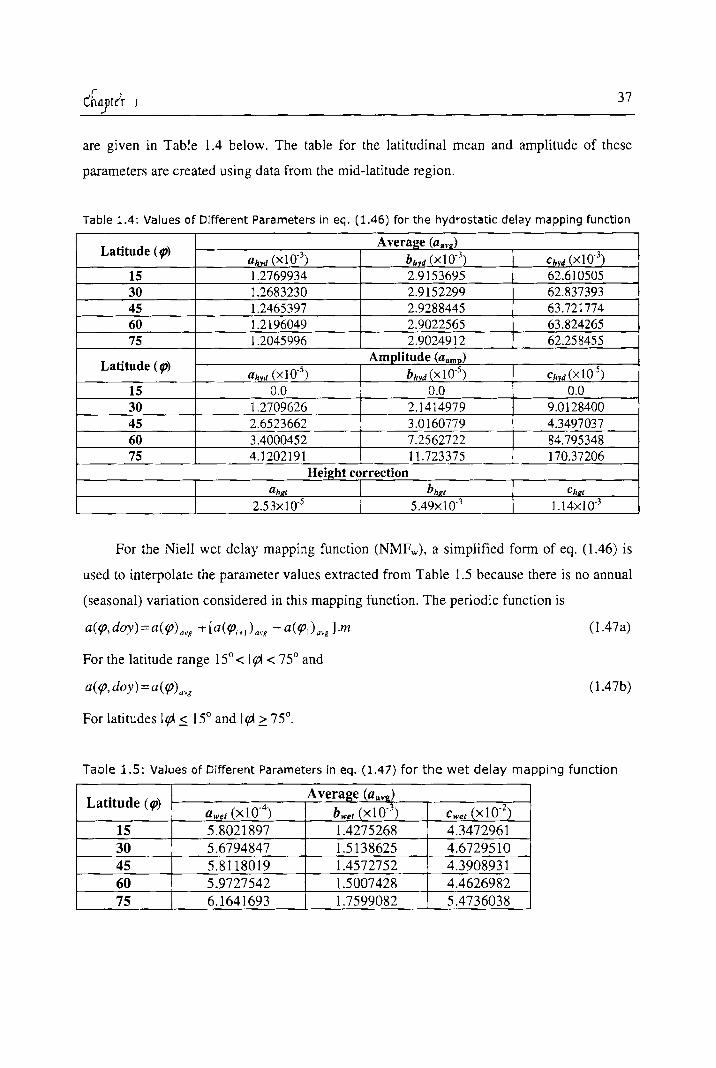
37

are given in Table 1.4 below. The table for the latitudinal mean and amplitude of these

parameters are created using data from the mid-latitude region.

Table 1.4: Values of Different Parameters in eq. (1.46) for the hydrostatic delay mapping function

Latitude (tp) A vera2e (am)

ahvd (x 1 0.3) bhvd (x 1 0.3) Chyd (x 1 0.3

)

15 1.2769934 2.9153695 62.610505 30 1.2683230 2.9152299 62.837393 45 1.2465397 2.9288445 63.721774 60 1.2l96049 2.9022565 63.824265 75 1.2045996 2.9024912 62.258455

Latitude (tp) Amplitude (aamD)

ahvd (x 10.5) bifyd (x 10's ) Chyd (x lO-5) 15 0.0 0.0 0.0 30 1.2709626 2.1414979 9.0128400 45 2.6523662 3.0160779 4.3497037 60 3.4000452 7.2562722 84.795348 75 4.1202191 11.723375 170.37206

Height correction ahJlI blW Ch.zl

2.53x10,5 5.49xl0·3 1.14xlO·3

For the Nie11 wet delay mapping function (NMFw), a simplified form of eq. (1.46) is

used to interpolate the parameter values extracted from Table 1.5 because there is no annual

(seasonal) variation considered in this mapping function. The periodic function is

(1.47a)

For the latitude range 15° < ItP < 75° and

a( <p, doy) = a( <P)avg (1.47b)

For latitudes I tP ::; 15° and I tP ~ 75°.

Table 1.5: Values of Different Parameters in eq. (1.47) for the wet delay mapping function

Latitude (tp) Average (aavl!)

awet (x 10'4) bWel (x 10'3) Cwet (x 10'2) 15 5.8021897 1.4275268 4.3472961 30 5,6794847 1.5138625 4.6729510 45 5.8118019 1.4572752 4.3908931 60 5.9727542 1.5007428 4.4626982 75 6.1641693 1.7599082 5.4736038

As there is no height correction term in the wet delay the NMFw reduces to

ah,'d 1+------bh)'d

1+--1 + C"yd

MFw(X) = ------=----ahyd

cos(x) + b hyd cos(x) + .

cos (X) + C hyd

1.7.3 Global Mapping Function

38

(1.48)

The Global mapping function (GMF), which uses the same continued fraction as that

in NMF (eq. 1.45), is modeled with sufficient accuracy for zenith angles up to 87°. The

parameters a, band c, which are different for the hydrostatic and wet components are

computed from Numerical Weather Models. Using a 15° x 15° global grids of monthly mean

profiles for pressure, temperature and humidity from 40 years' ECMWF (European Centre

for Medium-range Weather Forecasts) reanalysis data (ERA40), the coefficients ahyd and awer

are determined. Taking pre-defined (empirical) expression for bhyd, Chyd, bwer. and ewer; the

coefficients ahyd and a Wel are derived through a single ray-trace at 3.3° initial elevation angle

(86.7° zenith angle) and by simply inverting the continued fraction form [Boehm et al.

2006a]. These hydrostatic coefficient (ahyd) at surface are then scaled down to mean sea level

(ao) using the height correction given by Niell [1996]. The mean values of 'ao' and its

amplitude are fitted using a periodic function (eq. 1.46a), to the time-series of the 'a'

parameters at each grid point. This global grid of the mean values, ao, and of its amplitude,

for both the hydrostatic and wet coefficients in the continued fraction form are expanded

into special spherical harmonic coefficients up to degree and order 9 in a least square

adjustment. This expansion is given as

9 n

ao = I I Pmn (sin qJ).[Anm . cos(m· A) + Bnn! . sin(m· A)] (1.49) n:O m:O

The hydrostatic and wet coefficients of 'a' for a given site coordinates and day-of-year can

then be determined using eq. (1.46).

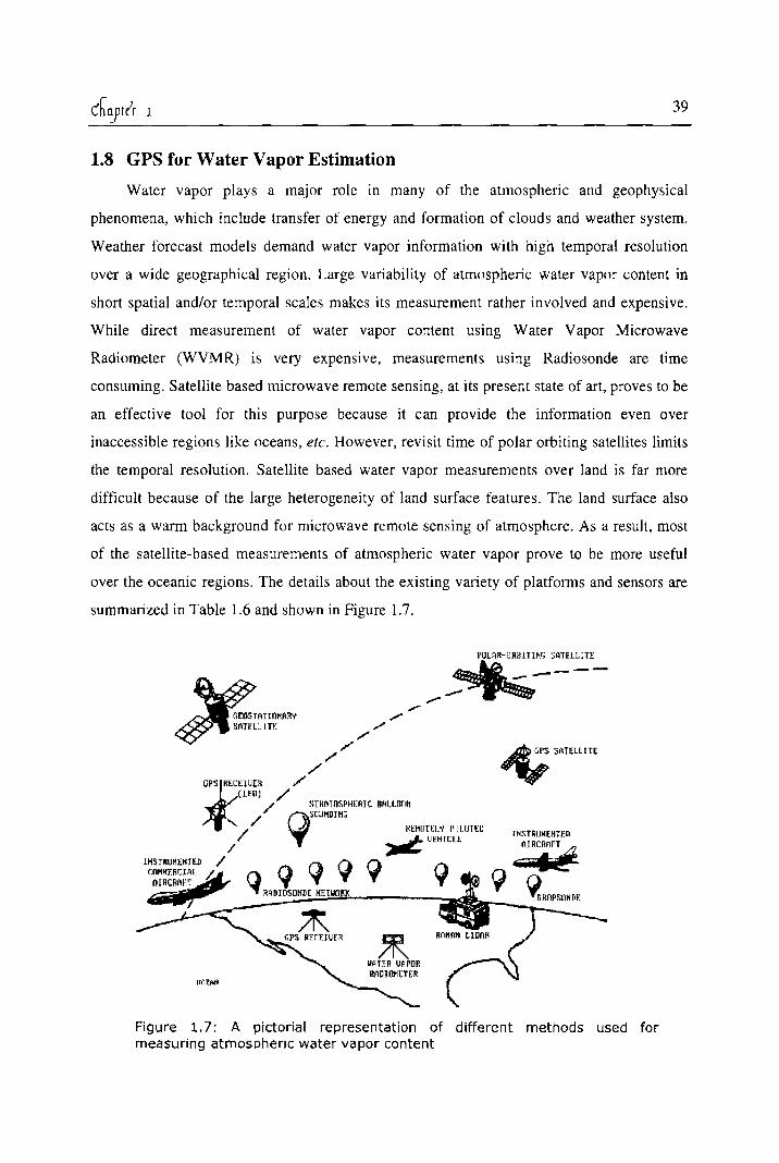
39

1.8 GPS for Water Vapor Estimation

Water vapor plays a major role in many of the atmospheric and geophysical

phenomena, which include transfer of energy and formation of clouds and weather system.

Weather forecast models demand water vapor information with high temporal resolution

over a wide geographical region. Large variability of atmospheric water vapor content in

short spatial and/or temporal scales makes its measurement rather involved and expensive.

While direct measurement of water vapor content using Water Vapor Microwave

Radiometer (WVMR) is very expensive, measurements using Radiosonde are time

consuming. Satellite based microwave remote sensing, at its present state of art, proves to be

an effective tool for this purpose because it can provide the information even over

inaccessible regions like oceans, etc. However, revisit time of polar orbiting satellites limits

the temporal resolution. Satellite based water vapor measurements over land is far more

difficult because of the large heterogeneity of land surface features. The land surface also

acts as a warm background for microwave remote sensing of atmosphere. As a result, most

of the satellite-based measurements of atmospheric water vapor prove to be more useful

over the oceanic regions. The details about the existing variety of platforms and sensors are

summarized in Table 1.6 and shown in Figure 1.7.

*':~'-"...--­/

./

,;' ,/

/

,.-./

l'PS RECEIU[lI /'

LEO) / / STRIlTOSPHI:HIC O~I.Ul(lH

/

/ 9S0UHDIHG REHnTELV PIWTrO / .",.t; UEHIClr

lHSTHUNIOHTED / () 9 COMHI:RCIAI. ~ Cl (} () y nIRCRilH~ .., Y tiiSii!V RADIDSOHD[ HETIIDRX

~'flULLlTE

INSTRIIHEHTf.D

:IR~

9 ~RnrsoNPE

Fig ure 1. 7: A pictorial representation of different methods used for measuring atmospheric water vapor content

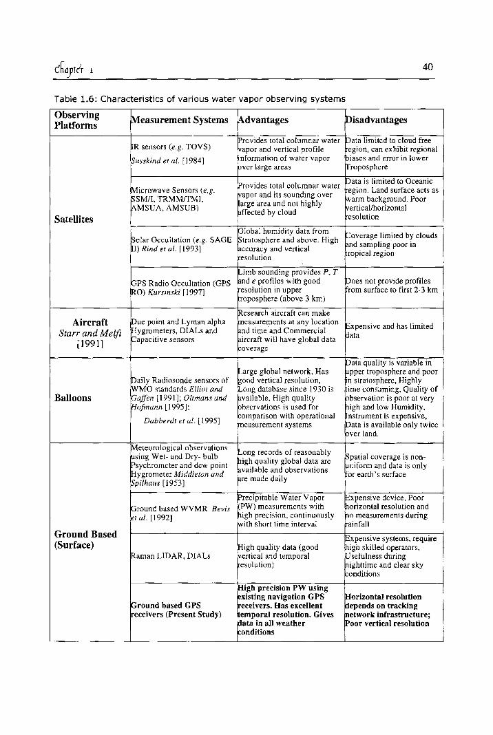
c~aJt(r 1 40

Table 1.6: Characteristics of various water vapor observing systems

Observing lMeasurement Systems Advantages !Disadvantages Platforms

Provides total columnar water lData limited to cloud free R sensors (e.g. TOVS) \lapor and vertical profile egion, can exhibit regional

~usskinde{al. [1984] ·nformation of water vapor ~iases and error in lower pver large areas [rroposphere

lMicrowave Sensors (e.g. Provides total columnar water lData is limited to Oceanic

~apor and its sounding over egion. Land surface acts as

~SMlI, TRMM/TMI, arge area and not highly iwarm background. Poor

lAM SUA, AMSUB) ~frected by cloud

ivertical/horizontal

Satellites esolution

~olar Occultation (e.g. SAGE plobal humidity data from ~ovcrage limited by clouds ~tratosphere and above. High

I) Rind et al. [1993] accuracy and vertical ~lnd sampling poor in

esolution ropical region

i'-'imb sounding provides P, T roes not provide profiles pPS Radio Occultation (GPS and e profiles with good

IRO) Kursinski [1997] esolution in upper rom surface to first 2-3 km roposphere (above 3 km)

lDue point and Lyman alpha ~esearch aircraft can make

Aircraft ~easurements at any location !Expensive and has limited

Starr and Melfi iHygrometers, DIALs and ~nd time and Commercial ~ata [1991 ] ~apacitive sensors ~ircraft will have global data

overage

lData quality is variable in

!Daily Radiosonde sensors of i'-'arge global network, Has iupper troposphere and poor ~ood vertical resolution, ·n stratosphere, Highly

IWMO standards Elliot and J..,ong database since 1930 is ime consuming, Quality of Balloons paffell [1991]; Oltmansand ~vailable, High quality pbservation is poor at very

lfIo/mann [1995]; pbscrvations is used for ~igh and low Humidity,

Dabberdt et al. [1995] omparison with operational nstrument is expensive,

measurement systems !Data is available only twice pver land.

!Meteorological observations Long records of reasonably

~patial coverage is non-~sing Wet- and Dry- bulb high quality global data are IPsychrometer and dew point iuniform and data is only !Hygrometer Middleton and

available and observations or earth's surface

~pilhaus (1953] fire made daily

Precipitable Water Vapor ~xpensive device, Poor

pround based WVMR Bevis PW) measurements with ~orizontal resolution and

~t ul. [1992] ~igh precision, continuously ,",0 measurements during with short time interval ainfall

Ground Based ~xpensive systems, require (Surface) High quality data (good high skilled operators,

iRaman LlDAR, DIALs vertical and temporal ~sefulness during esolution) righttime and clear sky

onditions

High precision PW using ~orizontal resolution

~round based GPS existing navigation GPS eceivers. Has excellent ~epends on tracking

eceivers (Present Study) emporal resolution. Gives network infrastructure; data in all weather Poor vertical resolution onditions

chaytcr 1 41

A local network of GPS receivers is an effective alternative for water vapor remote sensing

over the land [Businger et al., 1996] and this recently developed technique proves to be very

effective in measuring Precipitable Water vapor (PW), which is the height of the liquid

water column when the entire water vapor in a vertical column of the atmosphere is

condensed, as clouds and precipitation do not significantly affect the propagating GPS

signals at 19 and 24 cm wavelengths. Rocken et al. [1993; 1995; 1997] demonstrated the

capability of ground based GPS system for measuring PW with an accuracy of few

millimeters. Emardson et al. [1998] and Tregoning et al. [1998] also have reported similar

measurements of PW from GPS observations. However, most of these studies have been

carried out over the mid-latitude regions where the average PW is <20 mm. This points the

importance of PW measurements using GPS over tropical region, where the atmospheric

water vapor content is relatively large and perpetual cloud cover and precipitation severely

affect other remote sensing techniques.

The sensitivity of atmospheric refractivity to the presence of water vapor makes it

possible for ground-based GPS receivers to provide time series data on PW above the

receiver site. The wet component of propagation delay in microwaves, for a ground based

GPS receiver, is nearly proportional to the total amount of the water vapor (integrated) along

the signal path. In the case of liquid water and ice, the hydrogen bond between water

molecules greatly reduces the contribution of the dipole moment to the delay [Schiiler

2002}. Because of this, the presence of precipitation and cloud ice does not discernibly

affect the GPS measurement of water vapor. If the position of the receiver is accurately

known and the Ionospheric delay has been accounted with a fairly good accuracy, then it

will be possible to estimate the altitude integrated columnar water vapor overlying the

receiver from the GPS signals, making use of the data on surface pressure and temperature

at the same location [Bevis et al. 1992, 1994; Rocken et al. 1993, 1995; Duan et al. 1996].

As the Integrated water vapor is a representative of the total latent heat available in the

column, it can be used as a potential tool in numerical weather prediction (NWP) models

[Kuo et al., 1993, 1996] and weather analysis.

1.9 Motivations of this Study

Global Positioning System (GPS), with its high integrity, continuous availability and

reliability, revolutionized the navigation system based on radio ranging. With four or more

42

GPS satellites in view, a GPS receiver can find its location anywhere over the globe with

accuracy of few meters [Parkinson-Spilker et aI., 1996]. High accuracy - within

centimeters, or even millimeters is achievable by correcting the GPS signal with external

augmentation system. The use of satellite for critical application like navigation has become

a reality through the development of these augmentation systems (like W AAS, SDCM, and

EGNOS, etc.) with a primary objective of providing essential integrity information needed

for navigation service in their respective regions. Apart from these, many countries have

initiated developing space-based regional augmentation systems like GAGAN and IRNSS of

India, MS AS and QZSS of Japan, COMPASS of China, etc. In future, these regional

systems will operate simultaneously and emerge as a Global Navigation Satellite System or

GNSS to support a broad range of activities in the global navigation sector.

Among different types of error sources in the GPS precise positioning, the

propagation delay due to the atmospheric refraction is a limiting factor on the achievable

accuracy using this system. The W ADGPS, aimed for accurate positioning over a large area

though broadcasts different errors involved in GPS ranging including ionosphere and

troposphere errors, due to the large temporal and spatial variations in different atmospheric

parameters especially in lower atmosphere (troposphere), the use of these broadcasted

tropospheric corrections are not sufficiently accurate. This necessitated the estimation of

tropospheric error based on realistic values of tropospheric refractivity. Presently available

methodologies for the estimation of tropospheric delay are mostly based on the atmospheric

data and GPS measurements from the mid-latitude regions, where the atmospheric

conditions are significantly different from that over the tropics. No such attempts were made

over the tropics. In a practical approach when the measured atmospheric parameters are not

available analytical models evolved using data from mid-latitudes for this purpose alone can

be used. The major drawback of these existing models is that it neglects the seasonal

variation of the atmospheric parameters at stations near the equator. At tropics the model

underestimates the delay in quite a few occasions. In this context, the present study is afirst

and major step towards the development of models for tropospheric delay over the Indian

region which is a prime requisite for future space based navigation program (GAGAN and

IRNSS). Apart from the models based on the measured surface parameters, a region specific

model which does not require any measured atmospheric parameter as input, but depends on

43

latitude and day of the year was developed for the tropical region with emphasis on Indian

sector.

Large variability of atmospheric water vapor content in short spatial and/or temporal

scales makes its measurement rather involved and expensive. A local network of GPS

receivers is an effective tool for water vapor remote sensing over the land. This recently

developed technique proves to be an effective tool for measuring PW. The potential of using

GPS to estimate water vapor in the atmosphere at all-weather condition and with high

temporal resolution is attempted. This will be useful for retrieving columnar water vapor

from ground based GPS data. A good network of GPS could be a major source of water

vapor information for Numerical Weather Prediction models and could act as surrogate to

the data gap in microwave remote sensing for water vapor over land.

****