Propellant Injector Influence on Liquid-PropellantRocket Engine Instability

Pavel P. Popov,∗ William A. Sirignano,† and Athanasios Sideris‡

University of California, Irvine, Irvine, California 92697

DOI: 10.2514/1.B35400

The avoidance of acoustic instabilities, which may cause catastrophic failure, is demanded for liquid-propellant

rocket engines. This occurs when the energy released by combustion amplifies acoustic disturbances; it is therefore

essential to avoid such positive feedback. Although the energy addition mechanism operates in the combustion

chamber, the propellant injector system may also have considerable influence on the stability characteristics of the

overall system, with pressure disturbances in the combustion chamber propagating back and forth in the propellant

injector channels. The introduced time delaymay affect stability, depending on the ratio of thewave propagation time

through the injector to the period of the combustion chambers acousticmodes. This study focuses on transverse-wave

liquid-propellant rocket engine instabilities using a two-dimensional polar coordinate solver (with averaging in the

axial direction) coupled to one-dimensional solutions in each of the coaxial oxygen–methane injectors. A blockage in

one (or more) of the injectors is analyzed as a stochastic event that may cause an instability. A properly designed

temporary blockage of one or more injectors can also be used for control of an oscillation introduced by any physical

event. The stochastic and design variables parameter space is explored with the polynomial chaos expansionmethod.

Nomenclature

Achem = chemical rate constant, m3∕�s · kg�Aentrance = cross-sectional area of nozzle entrance, m2

Athroat = cross-sectional area of nozzle throat, m2

A, B = constants, defined in Eq. (2)a = speed of sound, m∕sa, b = chemical rate constantscp = specific heat at constant pressure, J∕K · kgcv = specific heat at constant volume, J∕K · kgD = mass diffusivity, m2∕sE = energy release rate, J∕kg · sj = index for Cartesian coordinatesL = chamber length, mL�·� = general differential operatorp = pressure, newton m−2

Q�d�l = Smolyak quadrature of lth order in d dimensionsR = chamber radius, mRs = mixture specific gas constant, J∕kg · KRi = inner radius of coaxial jet, mRo = outer radius of coaxial jet, mRu = universal gas constant, J∕kg · mole∕Kr = radial position, ms = specific entropy, J∕K · kgT = temperature, Kt = time, sU = coaxial jet velocity, m∕sur = radial velocity component, m∕suθ = tangential velocity component, m∕sYi = mass fraction of species iα, β = Schvab–Zel’dovich variablesγ = ratio of specific heatsϵ = activation energy, J∕kg · moleη = local radial coordinate for the injector grids

θ = azimuthal positionν = kinematic viscosity, m2∕sνT = turbulent kinematic viscosity, m2∕sξ = sample space coordinate of random variablesρ = density, kg · m−3

τF = first tangential mode period, sΨ�·� = Legendre polynomialsωi = reaction rate of species i, s−1

0 = undisturbed stateh· j ·i = inner product

Subscripts

F = fueli = index for chemical speciesj = index for Cartesian coordinatesm = properties in the intake manifoldO = oxidizer0 = undisturbed state

I. Introduction

W E ADDRESS the problem of liquid-propellant rocket engine(LPRE) combustion instability, which is a well-known

phenomenon in rocket operation. The high-energy release by com-bustion can, in certain conditions, reinforce acoustic oscillations,causing them to grow to destructive amplitudes. LPRE combustioninstability provides a very interesting nonlinear dynamics problem,as shown by both theory and experiment [1–3].

The combustion chamber, like any partially confined volume filledwith gas, has an infinite number of natural acoustic resonant modes.In some operational domains, linear theory can predict that any smalldisturbance in the noise range can grow to a finite-amplitude limit-cycle acoustic oscillation driven by the combustion process. Inanother type of operational domain, any disturbance, whether in thenoise range or substantially larger, will decay in time; the only limitcycle is the steady-state equilibrium. A third type of operationaldomain is one where both an unstable and a stable limit-cycleoscillation exist. That is, noise and larger disturbances up to somethreshold level will decay with time. However, above that thresholdlevel, disturbances will develop in time toward the stable limit-cycleoscillation, which has an amplitude higher than the threshold levelgiven by the unstable limit cycle. Our attention herewill focus on thisbistable operating domain of the engine where the triggering ispossible and both an unstable limit-cycle and a greater-amplitudestable limit cycle exist. Neighboring operating domains with

Presented as Paper 2014-0134 at the 52nd AIAA Aerospace SciencesMeeting, National Harbor, MD, 13–17 January 2014; received 3 April 2014;revision received 21 July 2014; accepted for publication 23 July 2014;published online 3 November 2014. Copyright © 2014 by the authors.Published by the American Institute of Aeronautics and Astronautics, Inc.,with permission. Copies of this paper may be made for personal or internaluse, on condition that the copier pay the $10.00 per-copy fee to the CopyrightClearance Center, Inc., 222 Rosewood Drive, Danvers, MA 01923; includethe code 1533-3876/14 and $10.00 in correspondence with the CCC.

*Postdoctoral Fellow; ppopov@uci.edu. Member AIAA.†Professor. Fellow AIAA.‡Professor.

320

JOURNAL OF PROPULSION AND POWER

Vol. 31, No. 1, January–February 2015

Dow

nloa

ded

by U

C I

RV

INE

on

Nov

embe

r 24

, 201

6 | h

ttp://

arc.

aiaa

.org

| D

OI:

10.

2514

/1.B

3540

0

D-149

different design parameters (e.g., mean pressure, mass flow, andmixture ratio) can be unconditionally stable (i.e., with no limit-cycleoscillation) or unconditionally unstable (i.e., with a stable limit-cycleoscillation). This is shown in Fig. 1, which shows calculation resultsbased on analyses given by Sirignano and Popov [3] and Popov et al[4]. It provides a stability diagram for a range of the injector velocityand reactant mixture fraction parameter variables. The top left graphshows values of the stable and unstable first tangential mode limitcycles as a function of the injector velocity. The top right graph showsvalues of the stable and unstable first tangential mode limit cycles as afunction of the inner injector radius, for a fixed outer injector radius(stoichiometric proportions are achieved for an inner injector radiusof 0.898 cm). The bottom graph shows a plot of stability regime typesas a function of both mixture fraction and injector velocity. For areduced injector velocity and very rich or very lean reactant mixtures,the overall system is unconditionally stable; and for an increasedinjector velocity at a stoichiometric mixture fraction, the overallsystem is unconditionally unstable.The design parameters remain constant with time; consequently,

drift will not occur from one domain to another during engineoperation.There are two general types of acoustical combustion instability:

“driven” instability and “self-excited” instability, as noted by Culick[5], who describes evidence in some solid-propellant rockets of thedriven type where noise or vortex shedding causes kinematic waves(i.e., waves carried with the moving gas) of vorticity or entropy totravel to some point where an acoustical reflection occurs. Thereflected wave causes more noise or vortex shedding after travelingback, and a cyclic character results. These driven types do not rely onacoustical chamber resonance and are much smaller in amplitude,since the energy level is limited by the driving energy. The frequencyof oscillation for cases where vortex shedding is a factor depends ontwo velocities: the sound speed and the subsonic, kinematic speedof the vortex. Consequently, the frequency is lower than a purelyacoustic resonant frequency. Oscillations of this type are found in thelongitudinal mode. To the best of our knowledge, these have neverbeen observed in LPRE operation or in any transverse-mode insta-

bility and, when occurring in solid rockets or ramjets, the amplitudesaremuch lower than the values of concern for LPRE. So, theywill notbe addressed in this research.Interest in propellant combinations of hydrocarbon fuel and

oxygen, stored as liquids, is returning in the LPRE field. Theanalysis and results here will address situations where the methaneand oxygen propellants are injected coaxially as gasses. Thesepropellants will have elevated temperatures at the injectors becausethey have been used before injection, either for partial combustion forgas generation to drive a turbo pump or as a coolant. In particular,the inlet temperature and the mean combustion-chamber pressurewere carefully chosen to place the mixture in the supercritical (i.e.,compressible fluid) domain. Therefore, realism is maintained herewhen the chamber flow is treated as gaseous.The dynamic coupling of the injector system with the combustion

chamber of a liquid-propellant rocket engine has been a topic ofinterest for many decades. Two types of instabilities are known tooccur. The chugging instability mode has nearly uniform but time-varying pressure in the combustion chamber. The combustion cham-ber acts as an accumulator or capacitor, whereas the inflowingpropellant mass flux oscillates because the oscillating chamberpressure causes a flux-controlling oscillatory pressure drop acrossthe injector. This low-frequency instability was characterizedby Summerfield [6]. The second type of coupling involves a high-frequency oscillation at a near-resonant chamber mode frequency.Here, the resonant frequency has beenmodestly adjusted because theacoustic system involves some portion of the internal volume of theinjector as well as the combustion chamber and convergent nozzlevolumes.Crocco andCheng [7] discussed both types of instability forone-dimensional (longitudinal) oscillations. Interesting discussionsof coupled injector-system acoustics by Nestlerode, Fenwick, andSack and by Harrje and Reardon can be found in pages 106–126 ofthe well-known NASA SP-194 [1]. More recent overviews andanalyses are provided by Hutt and Rocker [8] and DeBenedictus andOrdonneau [9]. Yang et al. [10] provided several interesting papers onthe design and modeling of rocket injector systems. Our work willfocus on the high-frequency coupling of the transverse chamber

150 200 250 3000

20

40

60

80

100

120

140

160

180

Injector velocity (m/s)

Lim

it-cy

cle

ampl

itude

(at

m)

Stable limit cycleUnstable limit cicle

0.05 0.06 0.07 0.08 0.09 0.1 0.110

20

40

60

80

100

120

140

160

Injector inner radius (m)

Lim

it-cy

cle

ampl

itude

(at

m)

Stable limit cycleUnstable limit cicle

0 0.5 1 1.5 2 2.5 3100

150

200

250

300

Mixture Fraction

Inje

ctor

Vel

ocity

(m

/s)

Unconditionally stable regimeTriggered instability regimeUnconditionally unstable regimeEstimated onset of triggered instability regimeEstimated onset of conditionally unstable regime

Fig. 1 System stability as a function of injector velocity and inner radius (mixture ratio).

POPOV, SIRIGNANO, AND SIDERIS 321

Dow

nloa

ded

by U

C I

RV

INE

on

Nov

embe

r 24

, 201

6 | h

ttp://

arc.

aiaa

.org

| D

OI:

10.

2514

/1.B

3540

0

oscillations with the injector but will differ from previous works intwoways. These previousworksmostly used linear analysis, whereaswe shall address the nonlinear dynamics. Furthermore, the analysishere will consider disruptions of the injector flow, both as potentialtriggers of nonlinear instability and as potential mechanisms forarresting a developing instability.The disturbances that trigger combustion instability can result

from fluid-mechanical disruptions in the propellant injection process,shedding in the combustion chamber of large rogue vortices thateventually flow through the choked nozzle [11], extraordinary excur-sions in local burning rates, or a synergism among such events. In thepresentwork,wewill consider the first of the aforementioned types ofdisturbances, namely, disturbances due to blockage in one or more ofthe injector ports. Such blockages are characterized by their mag-nitude, location, duration, and delay between each other. Typically,the rocket engineer does not know these characteristics a priori;therefore, these parameters bear uncertainty and may be described asstochastic variables. Thus, this nonlinear dynamics problem mayproperly be viewed as stochastic. In particular, the magnitude andduration of a blockage and, for the involvement ofmore than one port,the time delay between injector blockages are viewed as randomvariables.To obtain an accurate solution to this stochastic problem in an

efficient computational manner, we employ a polynomial chaosexpansion (PCE) [12,13] that expresses the solution as a truncatedseries of polynomials in the random variables (RVs) characterizinginjector blockage. The use of PCEs in terms of Hermite polynomialsof Gaussian RVs was introduced by Wiener [14], and their con-vergence properties were studied by Cameron and Martin [15].Nonlinear oscillations present a challenging application for PCEmethods, as they have difficulty with approximating the long-termsolution of dynamical equations; indeed, convergence of the PCE isnot uniform with respect to the time variable. As it will be discussedlater in detail, it is possible to capture the triggering of unstableoscillations with a modest number of terms in the PCE and do so at acomputational cost considerably smaller than a more traditionalMonte Carlo approach. Unlike the authors’ previous work [4], whichuses PCE exclusively for spanning the parameter space of randominjector channel blockages, the present research also uses the PCEmethodology to explore the parameter space of a single designvariable, namely, the length of the injector channel, which hassignificant influence on the stability characteristics of the overallsystem.In recent previous papers [3,4], a more detailed background and

literature review was presented for combustion instability researchand stochastic analysis. Consequently, a less detailed review isprovided here.In this paper, an analysis is presented of nonlinear transverse-mode

combustion instability in a circular LPRE combustion chamber withacoustic coupling to a quasi-steady exit flow through many short,convergent, choked nozzles distributed over the exit cross section. Inthis way, it is similar to previous analyses [3,4]. Although the nozzleconfiguration deviates from practical designs, it has a long history ofuse in experiments and theory on account of its convenience [1,7]. Anew aspect involves the nonlinear acoustic couplings with flowsin the propellant injectors upstream of the chamber. In addition,triggering is examined through a stochastic analysis following ourprevious approach [4]. In practice, propellant flow through the in-jector can be in the same liquid phase as the stored propellant: in agaseous form mixed with combustion products because of upstreamflow through a preburner used for a propellant turbopump, orin gaseous form because the liquid propellant was used as acombustion-chamber-wall coolant upstream. We consider heregaseous coaxial flow of the pure propellants methane and oxygen,based on the last scenario.The remainder of this paper is organized as follows: the governing

equations for the wave dynamics and the jet mixing and reaction areintroduced in Sec. II. The polynomial chaos expansion approx-imation to the stochastic solution is also described in Sec. II.Section III provides the details of the numerical solution and analyticexpressions for the stochastic disturbances to the flow that possibly

can trigger the large-amplitude transverse acoustic oscillation.Results are presented in Sec. IV.

II. Governing Equations

A. Deterministic Analysis

The present analysis focuses on pure tangential modes ofoscillation without significant longitudinal effects. We neglect theviscous and diffusion terms in the development of thewave equation,as these processes act onmuch smaller length scales than those of theacoustic waves in the combustion chamber. The wave equation forpressure is averaged in the axial x direction to yield the followingtwo-dimensional evolution equation for the longitudinal average ofpressure [3]:

∂2p∂t2� Ap�γ−1�∕2γ ∂p

∂t− Bp�γ−1�∕γ

�∂2p∂r2� 1

r

∂p∂r� 1

r2∂2p∂θ2

�

� �γ − 1�γ

1

p

�∂p∂t

�2

� �γ − 1� ∂E∂t

� γp�γ−1�∕γ�∂2�p1∕γu2r�

∂r2� 2

r

∂�p1∕γu2r�∂r

� 2

r

∂2�p1∕γuruθ�∂r∂θ

� 2

r2∂�p1∕γuruθ�

∂θ

� 1

r2∂2�p1∕γu2θ�

∂θ2−1

r

∂�p1∕γu2θ�∂r

�(1)

where r and θ are the radial and azimuthal coordinates, respectively;p denotes pressure; u denotes velocity; and γ is the specific heat ratio.E is the energy release rate, and A and B are constants dependent onthe steady-state temperature and pressure, and the ratio between thethroat and entrance areas of the nozzle:

B � a20

p�γ−1�∕γ0

A � KBL

K � γ � 1

2γ

Athroat

Aentrance

�γ

R

�1∕2�γ � 1

2

�−��γ�1�∕2�γ−1�� p�γ−1�∕2γ0

T1∕20

(2)

with p0, T0, and a0 denoting, respectively, the pressure, temperature,and speed of sound of the undisturbed chamber; and Athroat andAentrance are, respectively, the throat and entrance areas of the nozzle.Neglecting viscous dissipation and turbulence–acoustic inter-

actions, the two momentum equations are averaged in the axialdirection to yield [3]

∂ur∂t� ur

∂ur∂r� uθ

1

r

∂ur∂θ

−u2θr� C

p1∕γ∂p∂r� 0

∂uθ∂t� ur

∂uθ∂r� uθ

1

r

∂uθ∂θ� uruθ

r� C

rp1∕γ∂p∂θ� 0 (3)

with C � p1∕γ0 ∕ρ0.

It is desirable to use a physically reasonable but simple descriptionof the wave dynamics for the gaseous flow in each of the severalcoaxial injectors. More elaborate studies of individual injectors aregiven in [16–20]. In the injector feed pipes, variations in thetangential direction are neglected; pressure and velocity evolve viathe equations

∂2p∂t2

− a2∂2p∂x2� a2 ∂

2�ρu2�∂x2

−∂a2

∂t∂�ρu�∂x

(4)

∂u∂t� u ∂u

∂x� −

1

ρ

∂p∂x

(5)

322 POPOV, SIRIGNANO, AND SIDERIS

Dow

nloa

ded

by U

C I

RV

INE

on

Nov

embe

r 24

, 201

6 | h

ttp://

arc.

aiaa

.org

| D

OI:

10.

2514

/1.B

3540

0

which are solved on 10 separate one-dimensional grids, one for eachseparate injector channel. To ensure a sufficient pressure drop fromthe intake manifold to the injector channels so that pressure fluc-tuations in the channels do not cause reverse flow, each injector pipeis modeled as being connected to the intake manifold via an orifice ofarea AO smaller than the area AI of the injector itself. Denoting theintakemanifold pressure and sound speed aspm andam, respectively;andwith the convention that the injector channels each have lengthLIand span the interval [−LI , 0] in the x direction, the velocity at theorifice exit, assuming isentropic flow, is equal to

uorifice � cD × am

�����������2

γ − 1

s �����������������������������������������������1 −

�p�−LI; t�pm

��γ−1�∕γs(6)

where CD ∈ �0; 1� is a discharge coefficient accounting for flowfriction and separation. By conservation ofmass, themeanvelocity atthe intake manifold end of the injector channel is equal to

u�−LI; t� � cDAOAIam

�����������2

γ − 1

s �����������������������������������������������1 −

�p�−LI; t�pm

��γ−1�∕γs(7)

To obtain the energy release rate E, we introduce the Shvab–Zel’dovich variableα � YF − νYO, whereYF andYO are the fuel andoxidizer mass fractions, respectively, with ν being the fuel-to-oxygenmass stoichiometric ratio. The variable

β � �Q∕�cpTo��YF − T∕To � �p∕po��γ−1�∕γ

is introduced. The variables α, β, and YF evolve by the following setof scalar transport equations:

∂α∂t� ux

∂α∂x� uη

∂α∂η

−D�∂2α∂η2� 1

η

∂α∂η� ∂2α

∂x2

�� 0 (8)

∂β∂t� ux

∂β∂x� uη

∂β∂η

−D�∂2β∂η2� 1

η

∂β∂η� ∂2β

∂x2

�� 0 (9)

and

∂YF∂t� ux

∂YF∂x� uη

∂YF∂η

−D�∂2YF∂η2� 1

η

∂YF∂η� ∂2YF

∂x2

�� ωF

(10)

In the preceding equation, x and η are, respectively, the axial andradial coordinates of one of several axisymmetric cylindrical gridscoaxial with each injector, and the source term on the right-hand sideof Eq. (10), following a one-step irreversible Arrhenius chemicalmechanism, has the form

ωF � AchemρYOYFe−ϵ∕RuT

� AchempoνRsTo

p

po

YF�YF − α��Q∕cpTo�YF − β� �p∕po��γ−1�∕γ

× exp

�ϵ∕RuTo

�Q∕cpTo�YF − β� �p∕po��γ−1�∕γ�

(11)

where Achem is the chemical rate constant; ϵ is the activation energy;andRs andRu are, respectively, themixture specific and universal gasconstants. The present source term formulation has been comparedwith the classic Westbrook and Dryer one-step mechanism [21,22],which uses nonunitary exponents for the preexponential factors YO,YF, and no significant difference was observed for the present case.The axial and radial velocities in Eqs. (8–10) are obtained from a

solution of the variable-density Reynolds-averaged Navier–Stokesequations

ρ

�∂ux∂t� ux

∂ux∂x� uη

∂ux∂η

�� −

∂pl∂x� ρνT

�∂2ux∂x2� 1

η

∂∂η

�η∂ux∂η

��(12)

ρ

�∂uη∂t� ux

∂uη∂x� uη

∂uη∂η

�� −

∂pl∂η

� ρνT

�∂2uη∂x2� 1

η

∂∂η

�η∂uη∂η

�−uηη2

�(13)

which are solved on each injector grid, where pl�x; η; t� is a localhydrodynamic pressure for which the mean is by definition 0 andwhich has considerably lower magnitude than the injector pressurep�t� obtained from Eq. (1). The density in Eqs. (12) and (13) isobtained from the species scalars and the long-wavelength pressurep�t� at the injector’s location, so that the overall procedure for solvingEqs. (12) and (13) is elliptic.The turbulent viscosity νT and diffusivityD are evaluated based on

the turbulent viscosity approximation for a self-similar jet [23] with aturbulent Prandtl number of 0.7, yielding

νT �U�t�Ro35

(14)

D � U�t�Ro24.5

(15)

where U�t� is the magnitude of the vector formed by the jet exitvelocity and the local transverse-wave-induced velocity.

B. Galerkin Approximation of a Stochastic Partial DifferentialEquation System with Uncertainty in the Initial Conditions

We use the polynomial chaos expansion method, previouslyapplied by the authors in [4] to a similar problem dealing only withthe combustion-chamber wave dynamics. Let the perturbation fromsteady-state operating conditions be uniquely determined by a vector,ξ, of independent random variables or geometrical parameters, suchas the length of the injector pipe.Then, the solution of the system of partial differential equations

(PDEs) from the previous subsection, consisting of the fieldsp, ui, α,β, and YF may be expressed as a set of fields, in the forms �p; ui� �n�r; θ; t; ξ� and �α�j�; β�j�; Y�j�F � � m�x; η; t; ξ�, with the superscript�j� denoting each of the 10 injectors, and so the systemof Eqs. (1) and(3) forms two multivariate PDE systems [4]:

L1�n; r; θ; t; ξ� � f1�r; θ; t;m; ξ� (16)

L2�m; x; η; t; ξ� � f2�x; η; t;n; ξ� (17)

where Eq. (16) governs the evolution of p, ur, and uθ on a two-dimensional r − θ grid. Equation (17) governs the evolution of 10sets (one for each injector) of the fields α, β, and YF on two-dimensional x − η grids, coaxial with the injector axes. L1 and L2

are the differential operators representing Eqs. (1) and (3) andEqs. (8–10) respectively, and f1, f2 are source terms. Note thatEqs. (16) and (17) are coupled via the dependence on m of f1, thesource term in the evolution equation of n (due to the pressure beingdependent on the energy release) and, conversely, via the dependenceon n of f2 (due to the YF source term being dependent on pressure).We shall employ the stochastic Galerkin methodology toapproximate the solution of Eq. (16). For an in-depth introductionto the stochastic Galerkin technique, the reader is referred to [12,13].A truncated polynomial chaos expansion consists of the

approximations

POPOV, SIRIGNANO, AND SIDERIS 323

Dow

nloa

ded

by U

C I

RV

INE

on

Nov

embe

r 24

, 201

6 | h

ttp://

arc.

aiaa

.org

| D

OI:

10.

2514

/1.B

3540

0

n�r; θ; t; ξ� ≈XPk�0nk�r; θ; t�Ψk�ξ�

m�x; η; t; ξ� ≈XPk�0mk�x; η; t�Ψk�ξ� (18)

whereΨk�ξ� areP� 1Legendre polynomials in the random vector ξ.In particular, for the present case that uses uniform random variables,Ψk�ξ� are all possible n-dimensional products, of a degree up to l forthe lth-order PCE expansion, in the Legendre polynomials of thecomponent scalars of ξ. For a fixed simulation end time TF andadditional smoothness assumptions, this representation of the samplespace implies exponential [13] convergencewith respect to the order,l, of the PCE expansion. The number of polynomials,P� 1, is equalto �n� l�!∕�n!l!�. For the low-dimensional sample space used in thisstudy, the PCE methodology has substantially better computationalefficiency than a more standard Monte Carlo procedure [4].Substituting the approximation of Eq. (18) into Eqs. (16) and (17),

and taking the inner product denoted by h· j ·i over the range of ξwitheach of the polynomials Ψk�ξ�, yields

�L1

�r; θ; t; ξ;

XPk�0nk�r; θ; t�Ψk�ξ�

�jΨi�ξ�

�

� hf1�r; θ; t;m; ξ�jΨi�ξ�i (19)

�L2

�x; η; t; ξ;

XPk�0mk�x; η; t�Ψk�ξ�

�jΨi�ξ�

�

� hf2�x; η; t;n; ξ�jΨi�ξ�i (20)

which are two systems ofP� 1 deterministic equations, each similarto the system of equations [Eqs. (1–10)], which can be solvednumerically for each of the P� 1 coefficients nk�r; θ; t� andmk�x; η; t� using the same discretization schemes used for theapproximation of a deterministic solution to Eqs. (1–10).A sparse grid based on Smolyak’s quadrature rule is used to deal

with the integration of the nonlinear terms when evaluating the innerproducts of Eqs. (19) and (20). In particular, we use Q�1�i f to denotethe ith order of a univariate nested quadrature rule [24], i.e.,

Q�1�i f �Xj

qi;jf�xi;j� (21)

where qi;j and xi;j are, respectively, the weights and nodes of the ith-order univariate quadrature, with Q�1�0 f being identically zero.We use Q�d1� ×Q�d2�g to denote the product of the multivariate

quadratures Q�d1� and Q�d2�: the first of which integrates on the firstd1 arguments, and the second Qd2 of which integrates on the last d2arguments of a multivariate function g. Then, the d-dimensional, lthorder of the sparse Smolyak quadrature, denoted Q�d�l f, is definedrecursively as

Q�d�l f �Xli�1�Q�1�i −Q�1�i−1� ×Q

�d−1�l−i�1f (22)

With thismultidimensional quadrature, we can approximate the innerproduct of, for example, the source term ωF by expressing it as afunction ofm�ξ� and n�ξ�, which are obtained from the polynomialexpansion [Eq. (18)]. This gives us ωF�ξ�, and the inner producthωF�ξ�jΨk�ξ�i is approximated by

hωF�ξ�jΨk�ξ�i ≈Q�d�l �ωF�ξ�Ψk�ξ�� (23)

where the lth-order quadrature Q�d�l is used to integrate on the d-dimensional sample space variable ξ.

The use of the Smolyak quadrature yields, for smooth functions f,exponential convergence of the numerical error with respect to theorder l of the quadratureQ�d�l f. Further, since it is based on only thosepoints of the d-dimensional product of the univariate quadratures

Q�1�l which yield product quadratures of order l or less (whereas astandard d-dimensional product of the univariate quadratures yields

product quadratures of order ld), the Smolyak quadrature Q�d�l finvolves evaluation on considerably fewer points than a simpleproduct of univariate quadratures. To match the accuracy of theSmolyak quadrature to that of the PCE, we use the same order forboth; for the seventh-order four-dimensional case considered next, asimple product of the seventh-order 15-point nested univariatequadratures would require 154 � 50; 625 points, whereas theSmolyak quadrature yielded by Eq. (22) requires only 641 points.

III. Simulation

Combustion instability was studied over a range of operatingconditions for a 10-injector design by [3]. With varying mixtureratio or mass flow, three zones of stability type were found: stableoperation under any perturbation; linearly (spontaneously) unstablewith infinitesimal perturbation (noise) resulting in nonlinear limit-cycle oscillation; and an operating zonewhere triggering occurs witha disturbance above a threshold magnitude, leading to a nonlinearlimit-cycle oscillation, while a perturbation below the thresholddecays. Here, our stochastic analysis will focus on this last operatingregime where triggering action is possible.The present simulation uses a cylindrical chamber of axial length

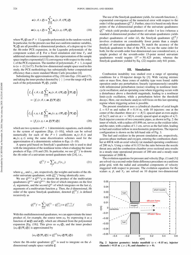
L � 0.5 m and radius R � 0.14 m, with 10 injectors: one at thecenter of the chamber; three at r � R∕2, spaced apart at even anglesof 2π∕3; and six at r � 3R∕4, evenly spaced apart at angles of π∕3.Each injector consists of two concentric pipes, as shown in Fig. 2: theinner of which, with a radius of 0.898 cm, serves as the oxidizer inlet;and the outer, with a radius of 1.1 cm, serves as the fuel inlet, leadingto fuel and oxidizer inflow in stoichiometric proportions. The injectorconfiguration is shown on the left-hand side of Fig. 3.The fuel and oxidizer in the present simulation are, respectively,

gaseous-phase methane and oxygen, entering the combustion cham-ber at 400 K with an axial velocity (at standard operating conditions)of 200 m∕s. Using a value of 0.115 for the ratio between the nozzlethroat area and the combustion-chamber cross-sectional area resultsin a steady-state operational pressure of 200 atm and a steady-statetemperature of 2000 K.The evolution equations for pressure and velocity [Eqs. (1) and (3)]

are solved via a second-order finite difference procedure on a uniformpolar grid, with the radial and azimuthal components of velocitystaggered with respect to pressure. The evolution equations for thescalars α, β, and YF are solved on 10 disjoint two-dimensional

−0.4 −0.2 0 0.2 0.4 0.6−0.05

−0.04

−0.03

−0.02

−0.01

0

0.01

0.02

0.03

0.04

0.05

x(m)

r(m

)

diffusion flame

diffusion flame

fuel

fuel

short nozzle

centerline

oxygen

Fig. 2 Injector geometry: intake manifold (x < −0.15 m), injectorchannels (−0.15 m ≤ x ≤ 0), and chamber (x > 0).

324 POPOV, SIRIGNANO, AND SIDERIS

Dow

nloa

ded

by U

C I

RV

INE

on

Nov

embe

r 24

, 201

6 | h

ttp://

arc.

aiaa

.org

| D

OI:

10.

2514

/1.B

3540

0

cylindrical grids (neglecting field variations in the azimuthal var-iable): each coaxial with the axis of the respective injector. For moredetails on the solution procedure for the deterministic system, thereader is referred to [3].The evolution equations for pressure and velocity in the injector

channels [Eqs. (4–7)] are solved on 10 separate one-dimensionalgrids for each injector channel (see Fig. 3). These solutions depend onthe tangential pressure and velocity solutions of Eqs. (1) and (3) fordetermination of the pressure value at the end of the injector channeland provide the injector outlet velocities for the evolution equationsfor the scalars α, β, and YF.In this study, we explore perturbations from standard operating

conditions due to blockages in the flow from the intake manifold tothe injector channels. Upstream of the injector channels, there existturbopumps and flow turns. These features can produce cavitation orshed vortices. Those disturbances can advect downstream and causeblockages entering the injector, which are modeled simply by abruptchanges in the discharge coefficient of Eq. (7) applied at the upstreamend of the injector channel. Specifically, we use an area ratio ofAO∕AI � 0.5 between the intake manifold orifice and the injectorchannel’s cross section. An unobstructed flow ismodeled byCD � 1for the discharge coefficient, and blockages are modeled as tem-porary decreases of the discharge coefficient to a certain minimalvalue. Specifically, a blockage of duration τB and peak mass flowreduction of k ∈ �0; 1� correspond to a decrease in the dischargecoefficient as a function of time according to the formula

cD � 1 − k sin �πt∕τB�2 (24)

We note that such a temporary reduction of the discharge coefficientcauses a decrease and subsequent increase in the propellant flow ratefor the corresponding injector, leading to a full sinusoidal cycle in therate of change of energy release, ∂E∂t , which appears as a source term inEq. (1). Thus, a blockage of period τ is expected to excite thecombustion chamber’s acoustic modes of similar period. To test thepossibility for excitation of higher tangential mode instabilities,deterministic simulations with a square pulse in the dischargecoefficient were also performed. Such a pulse contains higher-

frequency components, which specifically excite a second tangentialmode of considerable amplitude in the transient to the limit cycle.This component, however, decays by the time the limit cycle isachieved so that, for pulses with higher-frequency components, thelimit cycle (if one is achieved and the oscillation does not decay tothe standard operating conditions) is still dominated by the firsttangential acoustic mode of this chamber for the chosen designparameters.In addition to injector blockages as a source for triggered

instability, we explore their use as a mechanism for the reduction of agrowing instability. Specifically, we apply a controlled blockage aftera moderate interval of time (accounting for the delay inherent indetection of an instability and response to it) has elapsed since thetriggering event.

IV. Results

In this section, we explore the types of blockages that lead to thedevelopment of instabilities and their subsequent suppression. First,we present PCE simulations exploring a parameter space of possibleinjector disturbances that lead to instability. Then, we present resultsfrom simulations in which subsequent blockages, intentionallygenerated as part of a control mechanism, yield a return of thegrowing instability to the standard operating conditions.

A. Conditions Leading to the Development of a Limit Cycle

Here, we explore instabilities caused by a blockage in two adjacentinjector channels, namely, injectors 9 and 10, as identified in Fig. 3, inthe outer injector ring. We use the PCE methodology to obtainsolutions for a four-dimensional random variable ξ � �ξ1; ξ2; ξ3; ξ4�.The components ξ1; : : : ; ξ4 are independent and uniformlydistributed on the interval [0,1]; they determine the blockageduration and magnitude as defined in Eq. (24), the delay between theblockages of injectors 9 and 10, as well as the design parameter of theinjector length. Specifically, we have that ξ1 � k and τB ��0.5� ξ2�τF, where k and τB are, respectively, the blockage mag-nitudes and duration, as defined in Eq. (24); the delay between the

−0.1 −0.05 0 0.05 0.1

−0.1

−0.05

0

0.05

0.1

x(m)

y(m

)Polar grid for pressure/velocity

−0.02

0

0.02 −0.02

−0.01

0

0.01

0.02

0

0.001

0.002

0.003

0.004

0.005

0.006

0.007

0.008

0.009

0.01

loca

l y v

alue

(m)

Axisymmetric cylindrical grid for injectors

local x value(m)

Injector gridInner radius = 0.898 cmOuter radius = 1.1 cm

η

x

r

1θ

2

3

4

5

6

7

8

910

Fig. 3 Polar grid for chamber pressure and velocity. Axisymmetric grids for injector flows.

POPOV, SIRIGNANO, AND SIDERIS 325

Dow

nloa

ded

by U

C I

RV

INE

on

Nov

embe

r 24

, 201

6 | h

ttp://

arc.

aiaa

.org

| D

OI:

10.

2514

/1.B

3540

0

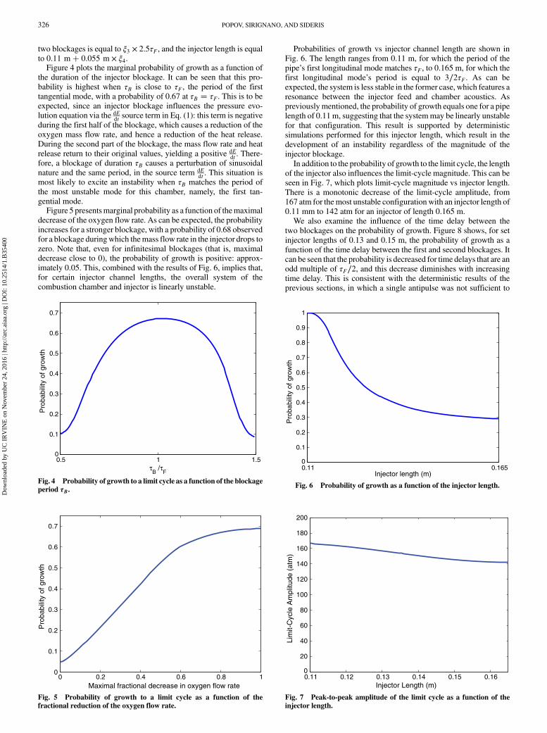
two blockages is equal to ξ3 × 2.5τF, and the injector length is equalto 0.11 m� 0.055 m × ξ4.Figure 4 plots the marginal probability of growth as a function of

the duration of the injector blockage. It can be seen that this pro-bability is highest when τB is close to τF, the period of the firsttangential mode, with a probability of 0.67 at τB � τF. This is to beexpected, since an injector blockage influences the pressure evo-lution equation via the dE

dt source term in Eq. (1): this term is negativeduring the first half of the blockage, which causes a reduction of theoxygen mass flow rate, and hence a reduction of the heat release.During the second part of the blockage, the mass flow rate and heatrelease return to their original values, yielding a positive dE

dt . There-fore, a blockage of duration τB causes a perturbation of sinusoidalnature and the same period, in the source term dE

dt . This situation ismost likely to excite an instability when τB matches the period ofthe most unstable mode for this chamber, namely, the first tan-gential mode.Figure 5 presentsmarginal probability as a function of themaximal

decrease of the oxygen flow rate. As can be expected, the probabilityincreases for a stronger blockage, with a probability of 0.68 observedfor a blockage duringwhich themass flow rate in the injector drops tozero. Note that, even for infinitesimal blockages (that is, maximaldecrease close to 0), the probability of growth is positive: approx-imately 0.05. This, combined with the results of Fig. 6, implies that,for certain injector channel lengths, the overall system of thecombustion chamber and injector is linearly unstable.

Probabilities of growth vs injector channel length are shown inFig. 6. The length ranges from 0.11 m, for which the period of thepipe’s first longitudinal mode matches τF, to 0.165 m, for which thefirst longitudinal mode’s period is equal to 3∕2τF. As can beexpected, the system is less stable in the former case, which features aresonance between the injector feed and chamber acoustics. Aspreviously mentioned, the probability of growth equals one for a pipelength of 0.11m, suggesting that the systemmay be linearly unstablefor that configuration. This result is supported by deterministicsimulations performed for this injector length, which result in thedevelopment of an instability regardless of the magnitude of theinjector blockage.In addition to the probability of growth to the limit cycle, the length

of the injector also influences the limit-cycle magnitude. This can beseen in Fig. 7, which plots limit-cycle magnitude vs injector length.There is a monotonic decrease of the limit-cycle amplitude, from167 atm for themost unstable configurationwith an injector length of0.11 mm to 142 atm for an injector of length 0.165 m.We also examine the influence of the time delay between the

two blockages on the probability of growth. Figure 8 shows, for setinjector lengths of 0.13 and 0.15 m, the probability of growth as afunction of the time delay between the first and second blockages. Itcan be seen that the probability is decreased for time delays that are anodd multiple of τF∕2, and this decrease diminishes with increasingtime delay. This is consistent with the deterministic results of theprevious sections, in which a single antipulse was not sufficient to

0 0.2 0.4 0.6 0.8 10

0.1

0.2

0.3

0.4

0.5

0.6

0.7

Pro

babi

lity

of g

row

th

Maximal fractional decrease in oxygen flow rate

Fig. 5 Probability of growth to a limit cycle as a function of thefractional reduction of the oxygen flow rate.

0.11 0.1650

0.1

0.2

0.3

0.4

0.5

0.6

0.7

0.8

0.9

1

Injector length (m)

Pro

babi

lity

of g

row

th

Fig. 6 Probability of growth as a function of the injector length.

0.11 0.12 0.13 0.14 0.15 0.160

20

40

60

80

100

120

140

160

180

200

Injector Length (m)

Lim

it-C

ycle

Am

plitu

de (

atm

)

Fig. 7 Peak-to-peak amplitude of the limit cycle as a function of theinjector length.

0.5 1 1.50

0.1

0.2

0.3

0.4

0.5

0.6

0.7

τB /τ

F

Pro

babi

lity

of g

row

th

Fig. 4 Probability of growth to a limit cycle as a function of the blockageperiod τB.

326 POPOV, SIRIGNANO, AND SIDERIS

Dow

nloa

ded

by U

C I

RV

INE

on

Nov

embe

r 24

, 201

6 | h

ttp://

arc.

aiaa

.org

| D

OI:

10.

2514

/1.B

3540

0

arrest the instability once it had grown considerably. We note that, inFig. 8, although the overall probability of growth is larger for themore unstable, shorter injector length, this case also yields a largerdecrease in the growth probability for delay times of 3τF∕2and 5τF∕2.The time delay between the two blockages also determines the type

of first tangential limit cycle, when one develops. In particular, when

the time delay is close to 0 (modulo τF), the limit cycle has the shapeof a standing wave; whereas for time delays closer (modulo τF) toτF∕6 and 5τF∕6, the limit cycle has the form of a spinning wave,traveling in the counterclockwise direction and clockwise direction,respectively.Figure 9 shows, for the injector length of 0.135 m, a pressure

contour plot of the fully developed limit cycle in the polar, axiallyaveraged acoustic solver grid, as well as a contour plot of temperaturein one of the cylindrical injector grids at standard operating con-ditions. The somewhat irregular shape of the pressure contour plot isdue to the fact that the limit cycle contains acoustic modes of loweramplitude, in addition to the first tangential: specifically, a secondtangential mode and a subharmonic; the reader is referred to [3] for adetailed spectral description of the acoustic limit cycle for thisconfiguration. On the temperature contour plot, a diffusion flame isseen to develop in the mixing layer between oxidizer, fuel, and hotcoflow streams.Figure 10 shows a snapshot of the pressure and velocity distri-

butions in one of the injectors at r � 3∕4R: a longitudinal acousticwave of length four times the injector length can be observed. Thisresult is consistent with a classical quarter-wave tube with one openend and one closed end.To explore interactions between other injector pairs, we perform a

set of lower-dimensional PCE simulations, in which the blockageduration is set to equal τF, and the rest of the sample space variablesvary in the same fashion as the simulation presented previously.Table 1 presents the sensitivity of each possible injector pair, in termsof the overall possibility of growth. As can be seen on this table, themost sensitive cases are those that feature at least one injector on theouter ring.We also note that the central injector has little effect on the

x(m)

y(m

)

−0.1 −0.05 0 0.05 0.1

−0.1

−0.05

0

0.05

0.1

160

180

200

220

240

260

280

300

x(m)

r(m

)

0.05 0.1 0.15 0.2 0.25 0.3 0.35 0.4

0.002

0.004

0.006

0.008

0.01

0.012

0.014

0.016

0.018

500

1000

1500

2000

2500

3000

3500

Pressure (atm) Temperature (K)

Fig. 9 Limit-cycle chamber pressure (left). Temperature on cylindrical grid at standard operation (right).

0 0.05 0.1150

200

250

x(m)

P(a

tm)

0 0.05 0.150

100

150

x(m)

u(m

/s)

Fig. 10 Axial plot of instantaneous pressure in outer injector at limit cycle (left). Axial plot of axial velocity in the injector at the same time (right).

0 0.5 1 1.5 2 2.50

0.1

0.2

0.3

0.4

0.5

0.6

0.7

Time delay of second blockage, normalized by τF

Pro

babi

lity

of g

row

th

Injector length 0.15mInjector length 0.13m

Fig. 8 Probability of growth as a function of the time delay between thetwo blockages.

POPOV, SIRIGNANO, AND SIDERIS 327

Dow

nloa

ded

by U

C I

RV

INE

on

Nov

embe

r 24

, 201

6 | h

ttp://

arc.

aiaa

.org

| D

OI:

10.

2514

/1.B

3540

0

stability of the system, with no possibility of growth to a limit cyclewhen both blockages occur in this injector.

B. Potential for Active Control and Suppression of the DevelopingLimit Cycle

In the previous subsection, we observed that blockages in one ormore of the offcenter injectors may lead to the development of aninstability.Here,we consider the potential for active control via inten-tionally generated blockages, in order to reduce a growing instabilityback to the initial operating conditions. We do not necessarily ad-vocate that injector blockagewould be an optimal or even acceptablemethod of control. Rather, the point is to show that a designeddisruption can be effective in countering a developing instability.First, we shall consider a set of deterministic simulations in whichtwo or more “pulses” are introduced into the chamber.Specifically, we shall denote a single pulse to be a blockage in

injector 9 (as labeled in Fig. 3), of duration τF and peak mass flowreduction of 90%, followed by a blockage in injector 10, of the sameduration and mass flow reduction. The time delay between these twoblockages is τF∕6, which, combined with the durations for τF chosenhere, causes the development of a traveling first tangential limit cycle.We are interested in using a similar pair of blockages (or more than

one pair) in order to suppress the growing instability and return the

system to standard operating conditions. To this end, simulationshave been performed in which an additional pair of blockages ininjectors 9 and 10 have been introduced to the system, with a timedelay from the first pair ranging between τF and 10τF (note that theminimal time delay of τF is dictated by the chosen blockagedurations). We consider these subsequent blockages to be “anti-pulses,” which can be viewed as a potential control mechanism forbringing the system back into its normal operating condition.It has been found that the subsequent pair of blockages can bring

the system back to the original operating conditions, but only if itoccurs soon after the first pulse and is approximately τF∕2 out ofphase with it. As can be seen in Fig. 11, a single antipulse with adelay of 3τF∕2 can arrest the growth of the developing instability.However, antipulses of longer time delay from the initial perturbation(even when they are τF∕2 out of phase with it) can only reduce themagnitude of the developing instability, after which it startsgrowing again.In Fig. 11, we see that, even though single antipulses with a delay

of 5τF∕2 and larger are unsuccessful in causing a decay to 200 atm,they do reduce the energy of the growing instability. This suggeststhat a combination ofmore than one antipulse can stabilize the systemeven after a long time delay. To explore this possibility, we havechosen the case with an antipulse for which the time delay is 17τF∕2,

Table 1 Summary of probabilities and types of instability encountered for all possibleinjector pairs (not including mirrored configurations)

Injector pair Probability of growth Standing wave Spinning wave

1-1 (both inner ring) 0 No No1-2 (inner/middle ring) 0.271 Yes No2-2 (same injector in middle ring) 0.245 Yes No2-3 (separate injectors in middle ring) 0.326 Yes Yes1-5 (inner and outer ring) 0.482 Yes No2-6 (middle and outer ring) 0.619 Yes Yes2-7 (middle and outer ring) 0.563 Yes Yes2-8 (middle and outer ring) 0.507 Yes No9-9 (same injector outer ring) 0.498 Yes No9-10 (separate injectors in outer ring) 0.671 Yes Yes9-5 (separate injectors in outer ring) 0.622 Yes Yes9-6 (opposite injectors in outer ring) 0.573 Yes No

0 0.002 0.004 0.006 0.008 0.01 0.0120

2

4

6

8

10

12

14x 10

3

Simulation time (s)

Single pulse (causing growth to instability)

Two antipulses that jointly cause grown instability to decay

Single antipulse (5/2 τF delay) that fails to arrest the grown instability

Single antipulse (3/2 τF delay) that arrests the instability before it has grown too much

L m

easu

re (

atm

)2

2

Fig. 11 L2 norm of pressure deviation from the standard operating condition of 200 atm, for a set of deterministic simulations with one or more injectorblockages in the outer ring.

328 POPOV, SIRIGNANO, AND SIDERIS

Dow

nloa

ded

by U

C I

RV

INE

on

Nov

embe

r 24

, 201

6 | h

ttp://

arc.

aiaa

.org

| D

OI:

10.

2514

/1.B

3540

0

and we have run a set of simulations adding an additional antipulse,with a delay of 19τF∕2 to 29τF∕2.The addition of the second antipulse can bring about a decay to

equilibrium, provided that it follows quickly after the first. Inparticular, additional antipulses for which the delay is either close to19τF∕2 or 21τF∕2 (the latter of which is shown in Fig. 11), canreinforce the first antipulse sufficiently to cause a decay to 200 atm.From these results, it can be concluded that a blockage in the

injector can act not only as a destabilizing mechanism but also as acontrol mechanism aimed at returning the combustion chamberback to its normal operating conditions once an instability has beendetected. Based on the results of the simulations presented here, thereare two possible avenues toward achieving this goal: either a singleblockage-induced antipulse that is introduced sufficiently quicklyafter the destabilizing event or a set of antipulses, close in time to eachother, to jointly reduce the energy of a higher-amplitude instability,after a longer time delay.Figure 12 provides contour plots of the simulation with a 3τF∕2

antipulse. In it, we can see the original spinning wave caused by thefirst pair of blockages and its disruption by the antipulse. The top leftplot shows the initial traveling wave caused by the first pair ofblockages. The top right plot shows the second blockage pairdisrupting the traveling wave. The bottom plot shows the decayingwave after antipulse caused by the second blockage pair. Theresulting pressure wave, in the shape of a first tangential spinningwave, has a magnitude below the triggering value and thus decays tozero amplitude at the mean value of 200 atm.To encompass a larger parameter space, we also present results for

a PCE simulation that, similar to the aforementioned deterministicresults, deals with two pairs of blockages, each of which takes placein injectors 9 and 10 with a time delay of τF∕6 between them. Thesample space variables are the magnitude of the first pair of block-

ages, which varies uniformly between 0 and 1; the magnitude of thesecond pair, similarly varying between 0 and 1; and the time delaybetween the two pairs ranging from 0 to 5τF∕2. First, we shallconsider the conditional probability that the second pulse will returnthe system to equilibrium, conditional upon the first pulse beingstrong enough to set up a limit cycle. Figure 13 plots the conditionalprobability of decrease to equilibrium as a function of the magnitudeof the second pulse pair: as can be expected, this probability increasesfor a stronger antipulse.

x(m)

y(m

)

−0.1 −0.05 0 0.05 0.1

−0.1

−0.05

0

0.05

0.1

170

180

190

200

210

220

230

x(m)

y(m

)

−0.1 −0.05 0 0.05 0.1

−0.1

−0.05

0

0.05

0.1

190

195

200

205

210

215

x(m)

y(m

)

−0.1 −0.05 0 0.05 0.1

−0.1

−0.05

0

0.05

0.1

194

196

198

200

202

204

206

Pressure (atm) Pressure (atm)

Pressure (atm)

Fig. 12 Pressure for decay toward normal conditions caused by antipulse of time delay 3τF∕2.

0 0.5 1 1.5 2 2.50

0.1

0.2

0.3

0.4

0.5

0.6

0.7

0.8

0.9

1

Delay between pulses

Con

ditio

nal p

roba

bilit

y of

dec

ay to

equ

ilibr

ium

Fig. 13 Conditional probability of decay to equilibrium as a function ofthe delay between pulse and antipulse.

POPOV, SIRIGNANO, AND SIDERIS 329

Dow

nloa

ded

by U

C I

RV

INE

on

Nov

embe

r 24

, 201

6 | h

ttp://

arc.

aiaa

.org

| D

OI:

10.

2514

/1.B

3540

0

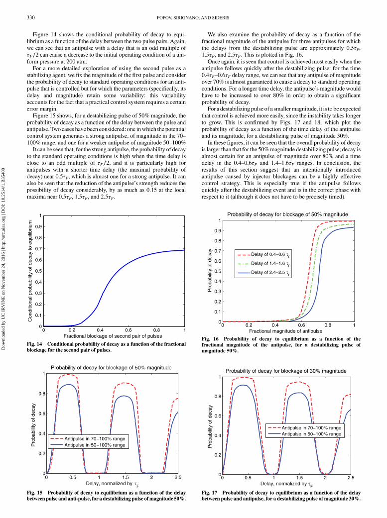
Figure 14 shows the conditional probability of decay to equi-librium as a function of the delay between the two pulse pairs. Again,we can see that an antipulse with a delay that is an odd multiple ofτF∕2 can cause a decrease to the initial operating condition of a uni-form pressure at 200 atm.For a more detailed exploration of using the second pulse as a

stabilizing agent, we fix the magnitude of the first pulse and considerthe probability of decay to standard operating conditions for an anti-pulse that is controlled but for which the parameters (specifically, itsdelay and magnitude) retain some variability: this variabilityaccounts for the fact that a practical control system requires a certainerror margin.Figure 15 shows, for a destabilizing pulse of 50% magnitude, the

probability of decay as a function of the delay between the pulse andantipulse. Two cases have been considered: one inwhich the potentialcontrol system generates a strong antipulse, of magnitude in the 70–100% range, and one for a weaker antipulse of magnitude 50–100%It can be seen that, for the strong antipulse, the probability of decay

to the standard operating conditions is high when the time delay isclose to an odd multiple of τF∕2, and it is particularly high forantipulses with a shorter time delay (the maximal probability ofdecay) near 0.5τF, which is almost one for a strong antipulse. It canalso be seen that the reduction of the antipulse’s strength reduces thepossibility of decay considerably, by as much as 0.15 at the localmaxima near 0.5τF, 1.5τF, and 2.5τF.

We also examine the probability of decay as a function of thefractional magnitude of the antipulse for three antipulses for whichthe delays from the destabilizing pulse are approximately 0.5τF,1.5τF, and 2.5τF. This is plotted in Fig. 16.Once again, it is seen that control is achievedmost easily when the

antipulse follows quickly after the destabilizing pulse: for the time0.4τF–0.6τF delay range, we can see that any antipulse of magnitudeover 70% is almost guaranteed to cause a decay to standard operatingconditions. For a longer time delay, the antipulse’s magnitude wouldhave to be increased to over 80% in order to obtain a significantprobability of decay.For a destabilizing pulse of a smallermagnitude, it is to be expected

that control is achieved more easily, since the instability takes longerto grow. This is confirmed by Figs. 17 and 18, which plot theprobability of decay as a function of the time delay of the antipulseand its magnitude, for a destabilizing pulse of magnitude 30%.In these figures, it can be seen that the overall probability of decay

is larger than that for the 50%magnitude destabilizing pulse; decay isalmost certain for an antipulse of magnitude over 80% and a timedelay in the 0.4–0.6τF and 1.4–1.6τF ranges. In conclusion, theresults of this section suggest that an intentionally introducedantipulse caused by injector blockages can be a highly effectivecontrol strategy. This is especially true if the antipulse followsquickly after the destabilizing event and is in the correct phase withrespect to it (although it does not have to be precisely timed).

0 0.5 1 1.5 2 2.50

0.2

0.4

0.6

0.8

1

Delay, normalized by τF

Pro

babi

lity

of d

ecay

Probability of decay for blockage of 50% magnitude

Antipulse in 70−100% rangeAntipulse in 50−100% range

Fig. 15 Probability of decay to equilibrium as a function of the delaybetweenpulse and anti-pulse, for a destabilizing pulse ofmagnitude 50%.

0 0.2 0.4 0.6 0.8 10

0.1

0.2

0.3

0.4

0.5

0.6

0.7

0.8

0.9

1

Fractional magnitude of antipulse

Pro

babi

lity

of d

ecay

Probability of decay for blockage of 50% magnitude

Delay of 0.4−0.6 τF

Delay of 1.4−1.6 τF

Delay of 2.4−2.5 τF

Fig. 16 Probability of decay to equilibrium as a function of thefractional magnitude of the antipulse, for a destabilizing pulse ofmagnitude 50%.

0 0.5 1 1.5 2 2.50

0.2

0.4

0.6

0.8

1

Delay, normalized by τF

Pro

babi

lity

of d

ecay

Probability of decay for blockage of 30% magnitude

Antipulse in 70−100% rangeAntipulse in 50−100% range

Fig. 17 Probability of decay to equilibrium as a function of the delaybetween pulse and antipulse, for a destabilizing pulse of magnitude 30%.

0 0.2 0.4 0.6 0.8 10

0.1

0.2

0.3

0.4

0.5

0.6

0.7

0.8

0.9

1

Fractional blockage of second pair of pulses

Con

ditio

nal p

roba

bilit

y of

dec

ay to

equ

ilibr

ium

Fig. 14 Conditional probability of decay as a function of the fractionalblockage for the second pair of pulses.

330 POPOV, SIRIGNANO, AND SIDERIS

Dow

nloa

ded

by U

C I

RV

INE

on

Nov

embe

r 24

, 201

6 | h

ttp://

arc.

aiaa

.org

| D

OI:

10.

2514

/1.B

3540

0

V. Conclusions

The method of stochastic simulation via polynomial chaosexpansion for a LPRE combustion chamber, previously developedand described by Popov et al. [4], has been extended to include theeffects of the injector feed system. A single blockage in the oxygenflow of an offcenter injector can cause the development of a standingwave first-tangential-mode limit cycle. Subsequent blockages,introduced either by accident or intentionally, can either modify thenature of the limit cycle to a traveling wave or bring about a decay ofthe limit cycle to the initial operating uniform pressure of 200 atm.The capability of subsequent antipulses to bring about a decay of

the instability decreases, as more time elapses since the triggeringevent. For a case in which considerable time has elapsed sincetriggering, and the instability has grown in magnitude, a singleantipulse is not sufficient to cause a decay of the instability, but twoantipulses closely following each other may have the desired effect.It is found that the length of the injector channels have considerable

influence on the stability characteristics of the system. When thechannel’s first longitudinal resonant mode is close in period to thefirst tangential mode of the combustion chamber, the injectors have adestabilizing effect, with higher probability for the development of alimit cycle, and a higher magnitude of the limit cycle than when theperiod of the injector’s first longitudinal mode equals 3τF∕2.Overall, stochastic simulation via the PCE method provides a

useful tool for the analysis of this highly complex system and fordetermining possible routes to control the development ofinstabilities in the LPRE combustion chamber.

Acknowledgments

This research was supported by the U.S. Air Force Office ofScientific Research under grant FA9550-12-1-0156 with MitatBirkan as the Program Manager.

Reference

[1] Harrje, D., and Reardon, F. (eds.), “Liquid Propellant RocketCombustion Instability,”NASA TR-SP-194, U.S. Government PrintingOffice, 1972, Chap. 3.

[2] Oefelein, J. C., and Yang, V., “Comprehensive Review of Liquid-Propellant Combustion Instabilities in F-1 Engines,” Journal of

Propulsion and Power, Vol. 9, No. 5, 1993, pp. 657–677.doi:10.2514/3.23674

[3] Sirignano, W. A., and Popov, P. P., “Two-Dimensional Model forLiquid-Rocket Transverse Combustion Instability,” AIAA Journal,Vol. 51, No. 12, 2013, pp. 2919–2934.doi:10.2514/1.J052512

[4] Popov, P. P., Sideris, A., and Sirignano,W. A., “StochasticModelling ofTransverse Wave Instability in a Liquid Propellant Rocket Engine,”

Journal of Fluid Mechanics, Vol. 745, April 2014, pp. 62–91.doi:10.1017/jfm.2014.96

[5] Culick, F. E. C., Unsteady Motions in Combustion Chambers for

Propulsion Systems, AGARDograph AG-AVT-039, NATO,Neuilly-sur-Seine, France, 2006.

[6] Summerfield, M., “A Theory of Unstable Combustion in LiquidPropellant Rocket Motors,” Journal of the American Rocket Society,Vol. 21, No. 5, 1951, pp. 108–114.doi:10.2514/8.4374

[7] Crocco, L., and Cheng, S.-I., Theory of Combustion Instability in LiquidPropellant Rocket Motors, AGARD Monograph 8, Butterworths,London, 1956.

[8] Hutt, J. J., and Rocker, M., “High-Frequency Injector-CoupledCombustion Instability,” Liquid Rocket Engine Combustion Instability,edited byYang,V., andAnderson,W.,Vol. 169, Progress inAstronauticsand Aeronautics, AIAA, Washington, D.C., 1995, pp. 345–376.

[9] DeBenedictus, M., and Ordonneau, G., “High Frequency InjectionCoupled Combustion Instabilities Study of Combustion Chamber/FeedSystem Coupling,” Joint Propulsion Conference, AIAA Paper 2006-4721, 2006.

[10] Yang, V., Habiballah, M., Hulba, J., and Popp, M. (eds.), Liquid RocketCombustion Devices: Aspects of Modeling, Analysis, and Design,Vol. 200, Progress in Astronautics and Aeronautics Series, AIAA,Reston, VA, 2005, Chaps. 1, 2, 4.

[11] Swithenbank, J., and Sotter, G., “Vortex Generation in Solid PropellantRocket,” AIAA Journal, Vol. 2, No. 7, 1964, pp. 1297–1302.doi:10.2514/3.2535

[12] Xiu,D., andKarniadakis, G., “TheWiener-AskeyPolynomialChaos forStochastic Differential Equations,” SIAM Journal on Scientific

Computing, Vol. 24, No. 2, 2002, pp. 619–644.doi:10.1137/S1064827501387826

[13] Xiu, D., Numerical Methods for Stochastic Computations: A Spectral

Method Approach, Princeton Univ. Press, Princeton, NJ, 2010, Chap. 6.[14] Wiener, N., “The Homogeneous Chaos,” American Journal of

Mathematics, Vol. 60, No. 4, 1938, pp. 897–936.doi:10.2307/2371268

[15] Cameron, R., and Martin, W., “The Orthogonal Development ofNonlinear Functionals in Series of Fourier-Hermite Functionals,”Annals of Mathematics, Vol. 48, No. 2, 1947, pp. 385–392.doi:10.2307/1969178

[16] Chehroudi, B., “Recent Experimental Efforts on High-PressureSupercritical Injection for Liquid Rockets and Their Implications,”International Journal of Aerospace Engineering, Vol. 2012, 2012,Paper 121802.doi:10.1155/2012/121802

[17] Davis, D. W., and Chehroudi, B., “Measurements in an Acoustically-Driven Coaxial Jet Under Supercritical Conditions,” Journal of

Propulsion and Power, Vol. 23, No. 2, 2007, pp. 364–374.doi:10.2514/1.19340

[18] Davis, D. W., and Chehroudi, B., “Shear-Coaxial Jets from a Rocket-Like Injector in a Transverse Acoustic Field at High Pressures,” 44th

AIAA Aerospace Sciences Meeting, AIAA Paper 2006-0758, 2006,pp. 9173–9190.

[19] Leyva, I. A., Chehroudi, B., and Talley, D., “Dark Core Analysis ofCoaxial Injectors at Sub-, Near-, and Supercritical Pressures in aTransverse Acoustic Field,” 43rd AIAA/ASME/SAE/ASEE Joint

Propulsion Conference and Exhibit, AIAA Paper 2007-5456, 2007,pp. 4342–4359.

[20] Tucker, P. K., Menon, S., Merkle, C. L., Oefelein, J. C., and Yang, V.,“Validation of High-Fidelity CFD Simulations for Rocket InjectorDesign,” 44th AIAA/ASME/SAE/ASEE Joint Propulsion Conference

and Exhibit, AIAA Paper 2008-5226, 2008.[21] Westbrook, C. K., and Dryer, F. L., “Simplified Reaction Mechanisms

for the Oxidation of Hydrocarbon Fuels in Flames,” Combustion

Science and Technology, Vol. 27, Nos. 1–2, 1981, pp. 31–43.doi:10.1080/00102208108946970

[22] Westbrook, C. K., and Dryer, F. L., “Chemical Kinetic Modeling ofHydrocarbon Combustion,” Progress in Energy and Combustion

Science, Vol. 10, No. 1, 1984, pp. 1–57.doi:10.1016/0360-1285(84)90118-7

[23] Pope, S. B., Turbulent Flows, Cambridge Univ. Press, NewYork, 2000,p. 162.

[24] Petras, K., “Smolyak Cubature of Given Polynomial Degree with FewNodes for Increasing Dimension,” Numerische Mathematik, Vol. 93,No. 4, 2003, pp. 729–753.doi:10.1007/s002110200401

E. KimAssociate Editor

0 0.2 0.4 0.6 0.8 10

0.1

0.2

0.3

0.4

0.5

0.6

0.7

0.8

0.9

1

Fractional magnitude of antipulse

Pro

babi

lity

of d

ecay

Probability of decay for blockage of 30% magnitude

Delay of 0.4−0.6 τF

Delay of 1.4−1.6 τF

Delay of 2.4−2.5 τF

Fig. 18 Probability of decay to equilibrium as a function of thefractional magnitude of the antipulse, for a destabilizing pulse ofmagnitude 30%.

POPOV, SIRIGNANO, AND SIDERIS 331

Dow

nloa

ded

by U

C I

RV

INE

on

Nov

embe

r 24

, 201

6 | h

ttp://

arc.

aiaa

.org

| D

OI:

10.

2514

/1.B

3540

0