properties of non-equilibrium states: dense colloidal
TRANSCRIPT

Properties of Non-Equilibrium
States:
Dense Colloidal Suspensions
under Steady Shearing
Dissertation
zur Erlangung des akademischen Grades des Doktors der
Naturwissenschaften an der Universitat Konstanz im FachbereichPhysik, Lehrstuhl Prof. Dr. Matthias Fuchs,
vorgelegt von
Matthias Helmut Gunter Kruger.
Tag der Einreichung: 9. Februar 2009
Tag der mundlichen Prufung: 9. April 2009
1. Referent: Prof. Dr. Matthias Fuchs2. Referent: Prof. Dr. Jorg Baschnagel

ii

Acknowledgments
A lot of people contributed to this thesis in different ways. First, I would like to thankProf. Matthias Fuchs for the opportunity to work under his supervision. I profittedenormously from his instructions and our discussions. He was always available whenI needed help. I also thank him for being very exacting concerning my results, whichforced me to optimize my arguments and helped me to separate helpful from meaninglessideas.
I am grateful to Prof. Jorg Baschnagel, the second referee of the thesis, for variousdiscussions. He made it possible for me to spend two inspiring months in his group atthe Institut Charles Sadron in Strasbourg for which I thank him.
I acknowledge financial support from the “Deutsche Forschungsgemeinschaft” in theInternational Research Training Group (IRTG) “Soft Condensed Matter”. The IRTGgave me the opportunity to participate in various seminars and workshops. I wouldalso like to thank the “Studienstiftung des deutschen Volkes” for its support and thepossibility to participate in several seminars for doctoral students.
I acknowledge the discussions with Dr. Joseph M. Brader on all kinds of topics as wellas the competitions on the badminton court. It was simply good to hear his opinion aboutthings. I also thank Dr. Thomas Voigtmann. For me, he is the “MCT-encyclopedia” ontwo legs and he immediately understands my points in our discussions.
Special thanks go to all my colleagues in the group who enriched the daily life. Dr. Tho-mas Voigtmann, Dr. Joseph M. Brader and Christof Walz are acknowledged for a criticalreading of the manuscript. I thank Fabian Weyßer for discussions within our beginningtheory-simulation collaboration.
I also acknowledge discussions with Prof. Jean-Louis Barrat, Prof. Michael E. Cates,Prof. Udo Seifert, Dr. Andrea Gambassi, Dr. Patrick Ilg and Dr. Igor Gazuz. Theyhelped me find my way through the FDT-violation jungle.
The members of the Baschnagel-group in Strasbourg made my stay there a greatpleasure for which I thank especially the young generation. I also acknowledge theinspiring discussions with Dr. Joachim Wittmer.
My parents, Dr. Ekkehard und Gisela Kruger, supported me in uncountable manyways for which I want to thank them.
Final and special thanks go to Anja Ging for her support, especially during the lastweeks. She is also acknowledged for a critical reading of the manuscript and commentsfrom the literature-studies point of view.
iii

iv

Contents
1 Introduction 11.1 Preamble . . . . . . . . . . . . . . . . . . . . . . . . . . . . . . . . . . . . 1
1.2 The System: Dense Colloidal Particles under Shear . . . . . . . . . . . . . 21.3 Microscopic Starting Point . . . . . . . . . . . . . . . . . . . . . . . . . . . 3
1.3.1 Low Density Limit – Taylor Dispersion . . . . . . . . . . . . . . . . 51.4 Integration Through Transients (ITT) Approach . . . . . . . . . . . . . . 6
1.5 Correlation Functions . . . . . . . . . . . . . . . . . . . . . . . . . . . . . 71.6 Mode Coupling Theory: Dynamics and Shear Stress . . . . . . . . . . . . 8
1.6.1 Density Correlations . . . . . . . . . . . . . . . . . . . . . . . . . . 81.6.2 Glass Transition and β-Analysis . . . . . . . . . . . . . . . . . . . 10
1.6.3 α-Scaling . . . . . . . . . . . . . . . . . . . . . . . . . . . . . . . . 111.6.4 Shear Stress . . . . . . . . . . . . . . . . . . . . . . . . . . . . . . . 12
1.6.5 Schematic Models . . . . . . . . . . . . . . . . . . . . . . . . . . . 12
2 Transient, Two-Time, and Stationary Correlators 152.1 Approximating the Exact Starting Point . . . . . . . . . . . . . . . . . . . 15
2.2 The Waiting Time Derivative . . . . . . . . . . . . . . . . . . . . . . . . . 172.3 Discussion of the Two-Time Correlator . . . . . . . . . . . . . . . . . . . . 20
2.4 Plotting the Waiting Time Dependent Curves Differently: Hypothesis ofNo Crossings . . . . . . . . . . . . . . . . . . . . . . . . . . . . . . . . . . 21
2.5 The Waiting Time Derivative Reconsidered . . . . . . . . . . . . . . . . . 23
2.5.1 Constraint for ∂∂tw
Cf(t, tw)∣∣∣tw=0
. . . . . . . . . . . . . . . . . . . . 23
2.5.2 Small-Shear Derivation Supporting the Approximation in Sec. 2.2 232.5.3 Why Our Findings for the Waiting Time Derivative Are Physically
Plausible . . . . . . . . . . . . . . . . . . . . . . . . . . . . . . . . 24
3 Incoherent Density Fluctuations 26
3.1 Previous Theoretical Studies on the Mean Squared Displacements underShear . . . . . . . . . . . . . . . . . . . . . . . . . . . . . . . . . . . . . . 26
3.2 Equation of Motion for the Transient Incoherent Correlator . . . . . . . . 273.3 β-Analysis . . . . . . . . . . . . . . . . . . . . . . . . . . . . . . . . . . . . 33
3.4 α-Scaling Equation . . . . . . . . . . . . . . . . . . . . . . . . . . . . . . . 343.5 Stationary Versus Transient Initial Decay Rate . . . . . . . . . . . . . . . 37
3.6 Mean Squared Displacements . . . . . . . . . . . . . . . . . . . . . . . . . 38
3.6.1 Neutral Direction . . . . . . . . . . . . . . . . . . . . . . . . . . . . 383.6.2 Gradient Direction . . . . . . . . . . . . . . . . . . . . . . . . . . . 39
v

Contents
3.6.3 Flow Direction . . . . . . . . . . . . . . . . . . . . . . . . . . . . . 403.6.4 Cross Correlation . . . . . . . . . . . . . . . . . . . . . . . . . . . . 42
3.7 Schematic Models . . . . . . . . . . . . . . . . . . . . . . . . . . . . . . . 44
3.7.1 (γ)-Sjogren Model . . . . . . . . . . . . . . . . . . . . . . . . . . . 443.7.2 Mean Squared Displacements . . . . . . . . . . . . . . . . . . . . . 44
3.8 Stationary Mean Squared Displacements . . . . . . . . . . . . . . . . . . . 48
4 Fluctuation Dissipation Relations under Steady Shear 51
4.1 Fluctuation Dissipation Theorem (FDT) and – Ratio (FDR) . . . . . . . 514.2 Previous Studies on the FDT in Non-Equilibrium . . . . . . . . . . . . . . 52
4.2.1 The General Formula for the Susceptibility in Non-Equilibrium . . 534.2.2 FDT Violation for a Single Driven Particle . . . . . . . . . . . . . 53
4.2.3 FDT Violation in Spin Glasses – Effective Temperature . . . . . . 53
4.2.4 Universal FDRs X = 12 in Spin Models . . . . . . . . . . . . . . . . 54
4.2.5 Simulation Results for the FDR under Shear and Further Works . 56
4.3 Linear Response and Susceptibility . . . . . . . . . . . . . . . . . . . . . . 564.4 Violation of Equilibrium FDT – Exact Starting Point . . . . . . . . . . . 58
4.5 Mode Coupling Approach . . . . . . . . . . . . . . . . . . . . . . . . . . . 59
4.5.1 Zwanzig-Mori Formalism – FDT Holds at t = 0 . . . . . . . . . . . 594.5.2 Second Projection Step . . . . . . . . . . . . . . . . . . . . . . . . 60
4.5.3 Markov Approximation – Long Time FDR . . . . . . . . . . . . . 614.5.4 FDT Violation Quantitative – Numbers for the FDR . . . . . . . . 62
4.5.5 FDT Violation Qualitative – Schematic Model F(FDR)12 . . . . . . . 66
4.5.6 FDR for Incoherent Fluctuations . . . . . . . . . . . . . . . . . . . 68
4.6 X = 12 Approach . . . . . . . . . . . . . . . . . . . . . . . . . . . . . . . . 72
4.6.1 The First Term as the Waiting Time Derivative . . . . . . . . . . . 72
4.6.2 The Other Terms . . . . . . . . . . . . . . . . . . . . . . . . . . . . 73
4.6.3 FD Relation under Shear . . . . . . . . . . . . . . . . . . . . . . . 734.6.4 Universal X = 1
2 Law . . . . . . . . . . . . . . . . . . . . . . . . . 74
4.6.5 Plotting the Final Susceptibilities . . . . . . . . . . . . . . . . . . . 744.6.6 FDR as Function of Shear Rate . . . . . . . . . . . . . . . . . . . . 76
4.6.7 FDR as Function of Wavevector . . . . . . . . . . . . . . . . . . . 76
4.6.8 Direct Comparison to Simulation Data . . . . . . . . . . . . . . . . 784.6.9 Universal FDR in the β-Regime . . . . . . . . . . . . . . . . . . . . 79
4.6.10 What Makes us Believe That Xf(t → ∞) ≤ 12 in the Glass? . . . . 80
4.6.11 Equilibrium FDT for Eigenfunctions . . . . . . . . . . . . . . . . . 81
4.6.12 FDT for the MSDs – Einstein Relation under Shear . . . . . . . . 824.7 Summary . . . . . . . . . . . . . . . . . . . . . . . . . . . . . . . . . . . . 85
5 Properties of the Stationary Correlator 875.1 Properties in Equilibrium . . . . . . . . . . . . . . . . . . . . . . . . . . . 87
5.2 Smoluchowski Versus Newtonian Dynamics . . . . . . . . . . . . . . . . . 875.3 Attempts to Show Properties for the Correlator under Shear . . . . . . . . 88
5.4 Splitting the SO Into Hermitian and Anti-Hermitian Part . . . . . . . . . 88
vi

Contents
5.5 Connection to the Susceptibility – The Comoving Frame . . . . . . . . . . 90
6 FDT-Violation: Final Discussion 936.1 Deterministic versus Stochastic Motion . . . . . . . . . . . . . . . . . . . . 936.2 What Does X(t → ∞) ≤ 1
2 Mean? . . . . . . . . . . . . . . . . . . . . . . 936.3 The Thesis in Short: A Toy Model . . . . . . . . . . . . . . . . . . . . . . 94
6.3.1 Shear Melts the Glass . . . . . . . . . . . . . . . . . . . . . . . . . 956.3.2 Dynamics . . . . . . . . . . . . . . . . . . . . . . . . . . . . . . . . 956.3.3 Mobility . . . . . . . . . . . . . . . . . . . . . . . . . . . . . . . . . 966.3.4 Long Time FDR . . . . . . . . . . . . . . . . . . . . . . . . . . . . 986.3.5 The Comoving Frame . . . . . . . . . . . . . . . . . . . . . . . . . 986.3.6 The Waiting Time Derivative . . . . . . . . . . . . . . . . . . . . . 99
7 Summary and Outlook 100
8 Zusammenfassung 102
A 104
B 106
C 109
Bibliography 111
vii


1 Introduction
1.1 Preamble
Paul is very drunk. He has lost control over his feet and his steps are random anduncorrelated. Because of this, it seems likely that Paul will move into the wrong directionand not find his way home. But since he is a physicist, he takes advantage of a veryfortunate coincidence: The street has a slight gradient pointing directly to his home. Heknows he is safe because, due to this gradient in the street, his walk is not completelyrandom. He will adopt a small mean velocity which will eventually lead him home.After some time he reaches a pedestrian crossing, where lots of people cross the street,their velocities being perpendicular to his. The density of the pedestrians is very highover an appreciably wide band. Paul enters the pedestrian band (he has no meansto prevent it). In the band he encounters many collisions with the pedestrians, theyare pushing him in arbitrary directions. Sometimes they even push him uphill, awayfrom his home. He realizes that his dynamics is now very fast due to the pushes by thepedestrians. But these pushes seem to be hardly influenced by the gradient of the street,his average velocity remains roughly unchanged. He starts wondering: “Am I violatingsome fundamental physics law?”
The expert reader has noticed that in the example above, the drunken walker missesthe heat bath, which is one of the important essences of the law he is violating; thefluctuation dissipation theorem (FDT). It is indeed a fundamental law that describesthe relation between thermal fluctuations (the random steps of the drunken walker)and the response to a small external force (the mean velocity due to the gradient inthe street). The law holds in equilibrium. In systems out of equilibrium, it does nothold in general. The drunken walker realizes that his fluctuations are stronger when heenters the (driven) pedestrian region, while his average velocity is roughly unchanged.The ratio of response and fluctuations is different compared to the case without thepedestrians.
In this thesis, we will investigate the violation of the fluctuation dissipation theo-rem for dense Brownian particles under shear near the glass transition. The study ismotivated by simulations [1] of this system, where a very peculiar violation of the the-orem was found: The non-equilibrium state seems to be characterized by a so calledeffective temperature that replaces the real temperature in the fluctuation dissipationtheorem. During the theoretical investigation of this phenomenon, it turned out thatthe description involves different correlation functions describing the fluctuations in thesheared system. After a general introduction of the system in this chapter, we willhence first study these different correlation functions and investigate their similaritiesand differences. Following this, we will study a specific class of observables, namely the
1

1 Introduction
fluctuations of a tagged particle and its mean squared displacement. These variableswere the focus of investigation in the simulations in Ref. [1]. In Chap. 3, we will studytheir dynamics which is necessary to be able to study their FDT version in Chap. 4.Considering the dynamics, we will additionally encounter an interesting effect, the par-ticle motion parallel to the shear direction is not diffusive at long times. This is knownas Taylor dispersion for low particle densities. But how will this relation look near theglass transition? In Chap. 4 we will finally turn to the fluctuation dissipation theoremand study its version for the system under shear. To a first approximation we find auniversal law for glassy states, which has intriguing similarities to the ones that werefound in non-equilibrium spin models. Our studies will yield results which are in goodagreement with the simulation results, differing only in one detail. This detail is impor-tant though, since our findings contradict the interpretation of this violation in terms ofan effective temperature. After this approximative treatment of the response functions,a more general and exact relation is derived in Chap. 5. It shows that the violation ofthe equilibrium FDT is connected to the non-Hermiticity of the time evolution opera-tor and gives further insights into the system under shear. In the last chapter finally,the physical reason for the violation of the equilibrium FDT will be illuminated. Thechapter closes with the study of a very simple toy model which allows to illustrate manyphenomena encountered in this thesis, thus contributing to their understanding.
1.2 The System: Dense Colloidal Particles under Shear
The system under consideration is a suspension of over-damped spherical Brownianparticles, so called colloids, interacting with each other via – in the simplest case – a hardsphere potential. At high density, this suspension is one of the most simple viscoelasticsystems, i.e., under external deformation it exhibits both dissipative behavior, like aNewtonian fluid, and elastic behavior, like a solid [2]. It is therefore often referred toas soft (metastable) solid and shows many interesting phenomena which will be brieflydiscussed below.
The Brownian particles are typically in the size range from a few nm to µm, i.e.,they are much larger than water molecules but still small enough to feel the thermalfluctuations. Since the observation timescale of the colloids is much larger than thetimescale on which the water molecules fluctuate, one can introduce an idealized picture,where the colloids are subject to short, random forces. The colloids thus perform randomwalks. Quantum effects play no role. Due to their mutual interactions, their motion ishindered and the dynamics is slowed down in comparison to an isolated particle. Thiseffect is the more drastic the higher the density of particles. At a certain density, theparticles hinder each other so much that they cannot get past each other any more andthe system freezes in; it undergoes a transition from an ergodic to a non-ergodic state,called the glass transition, which was verified for colloidal particles experimentally [3–9].If the system is monodisperse, i.e., all particles have the same size, it will crystallizebefore the glass transition density is reached. To avoid crystallization, one can forexample use particles with a small degree of polydispersity. In the glassy state, each
2
1.3 Microscopic Starting Point
particle is trapped in a cage formed by the surrounding particles. It is very hard oreven impossible to calculate the transition density exactly because it is a collectivephenomenon and cannot be treated by considering the motion of a single particle whilekeeping the other ones fixed. An approximate theory that very successfully describesthe glass transition is the mode coupling theory (MCT) [10].
Another phenomenon connected to the glass transition is aging; if the density of theparticles is increased rapidly (“quenched”) to the glassy phase (or if, for soft particlesthe temperature is rapidly decreased below the transition temperature), the system fallsout of equilibrium. It is not in the global energy minimum which it can reach onlyvery slowly due to its glassy nature. The outcome of measurements will depend on theamount of time elapsed since the quench; the system changes slowly with time, it “ages”.The described phenomenology can be found e.g. in Ref. [11].
While the glass transition of hard spheres (or of super-cooled liquids) has been studiedfor many years, it is still a great challenge to describe systems close to the glass transitionunder external driving. We will consider the simplest external driving, namely a steadyhomogeneous shear flow. This is currently also the subject of experimental studies [12–14]. We will consider space translationally invariant systems, where the gradient of theflow velocity of the particles is constant, i.e., we do not consider phenomena like shearbanding [15], where this is not the case. Also, the increase of the viscosity at highershear rates, the so called shear thickening [16] attributed to hydrodynamic interactions,and the jamming transition at somewhat higher densities and shear rates [11, 17] willnot be issues for our small-shear studies. For small shear rates, one usually observesshear thinning, i.e., the viscosity decreases with shear rate. Aging effects are absentin the time translationally invariant steady state under shear. See e.g. the reviews inRefs. [18, 19].
The sheared system under consideration hence reaches a steady state, but it is outof equilibrium. This causes many new and interesting phenomena. The system undershear is ergodic even when the un-sheared system is glassy, i.e., due to the shear, theparticles can explore all (phase-) space. The dynamics of the system is governed by shearat arbitrary small shear rates. Due to this, many observables are non analytic in shearrate which leads to non-trivial limiting values. The most famous example is the yieldstress, which will be introduced in Sec. 1.6.4. As we will see in Chap. 4, the violation ofthe fluctuation dissipation theorem also shows such a non-trivial limit in glassy states.
1.3 Microscopic Starting Point
We consider a system of N spherical particles of diameter d, dispersed in a solvent,see Fig. 1.1. The system has volume V . The particles have bare diffusion constantsD0 = kBTµ0, with mobility µ0 and kBT is the thermal energy. The interparticle forceacting on particle i (i = 1 . . . N) at position ri is given by Fi = −∂/∂riU(rj), where Uis the total potential energy. In an experimental system, also hydrodynamic interactionsbetween the particles are present [20]; if particle i moves, it causes the surroundingsolvent to move as well. The moving solvent affects the motion of the other particles,
3

1 Introduction
y
z x
Figure 1.1: The considered system: A dense colloidal suspension under shear. The spacialdirections are referred to as flow (x), gradient (y) and neutral (z) direction.
which in turn affects the solvent velocity and on this way particle i again. We will neglecthydrodynamic interactions to keep the theoretical description as simple as possible. Also,one assumes that they are less important for the slow glassy systems under consideration[18]. We will compare our results mostly to computer simulations, where hydrodynamicinteractions are absent.
The external driving, viz. the shear, acts on the particles via the solvent flow velocityv(r) = γyx, i.e., the flow points in x-direction and varies in the y-direction. γ is theshear rate. Due to the solvent velocity, the friction force of the solvent on particle i isnot proportional to its velocity, but proportional to the difference of this velocity to thesolvent velocity at ri. This leads to the equation of motion for the particles, namely theLangevin equation that misses in the over-damped system an inertia term,
∂ri
∂t− v(ri) = (Fi + fi) µ0. (1.1)
Different particles are coupled by the forces Fi. fi is the random force, representing thethermal activations by the solvent molecules. It satisfies (α and β denote directions)
⟨
fαi (t)fβ
j (t′)⟩
= 2kBT
µ0δαβδijδ(t − t′). (1.2)
Eq. (1.2) expresses that the random forces in different directions, on different particles,and at different times are uncorrelated. The pre-factor must be chosen such that the ran-dom force obeys the fluctuation dissipation theorem. One can show that from Eq. (1.2)the mean squared displacement of a free particle equals 2D0t. For the theoretical de-scription of the system it is more handy to use an equivalent formulation to Eq. (1.1),namely the Smoluchowski equation. It is an equation for the particle distribution func-
4

1.3 Microscopic Starting Point
tion Ψ(Γ ≡ ri, t) [20, 21],
∂tΨ(Γ, t) = Ω Ψ(Γ, t),
Ω = Ωe + δΩ =∑
i
∂i · [∂i − Fi − κ · ri] , (1.3)
with κ = γxy for the case of simple shear. Ω is called the Smoluchowski operator (SO)and it is built up by the equilibrium SO, Ωe =
∑
i ∂i · [∂i − Fi] of the system withoutshear and the shear term δΩ. We introduced dimensionless units d = kBT = D0 = 1,which will be used throughout the thesis unless stated otherwise. In contrast to Eq. (1.1),Eq. (1.3) has the advantage that it contains no random element. Nevertheless, it cannotbe solved exactly for the many particle system [22]. Without shear, the system reachesthe equilibrium distribution Ψe, i.e., ΩeΨe = 0. Under shear, the system is assumed toreach the stationary distribution Ψs with ΩΨs = 0. Ensemble averages in equilibriumand in the stationary state are denoted
〈. . . 〉 =
∫
dΓΨe(Γ) . . . , (1.4a)
〈. . . 〉(γ) =
∫
dΓΨs(Γ) . . . , (1.4b)
respectively. In the stationary state, the distribution function is constant but the systemis still not in thermal equilibrium due to the non-vanishing probability current jsi [21],
jsi = [−∂i + Fi + κ · ri]Ψs. (1.5)
In thermal equilibrium at γ = 0 the probability current vanishes, i.e., the system obeysdetailed balance [21]. In the steady state only the divergence of the current vanishes,not the current itself,
∑
i
∂i · jsi = −ΩΨs = 0. (1.6)
1.3.1 Low Density Limit – Taylor Dispersion
For the case of a single particle under shear, the Smoluchowski equation for the proba-bility density P (r, r0, t) can be solved and shall be shortly sketched here because we willcompare some of our results to the low density case. It reads (with restored units) [20]
∂
∂tP (r, r0, t) =
(
D0∂ · ∂ − γy∂
∂x
)
P (r, r0, t). (1.7)
For initial condition P (r, r0, 0) = δ(r − r0) one finds analytically,
P (r, r0, t) =1
8π3/2
√
D03t3(
γ2t2
12 + 1) exp
(−(
γ2t2
3 + 1)
(y − y0)2
4D0t(
γ2t2
12 + 1)
+γt(x − x0 − γty0)(y − y0) − (x − x0 − γty0)
2
4D0t(
γ2t2
12 + 1) − (z − z0)
2
4D0t
)
. (1.8)
5

1 Introduction
From this one can determine the mean squared displacements (MSDs) of the particle inthe different directions,
⟨(z − z0)
2⟩(γ)
=⟨(y − y0)
2⟩(γ)
= 2D0 t, (1.9a)⟨(x − x0)
2⟩(γ)
= 2D0 t + y20 γ2t2 +
2
3D0 γ2 t3. (1.9b)
〈(x − x0)(y − y0)〉(γ) = D0 γ t2. (1.9c)
The mean squared displacements in directions perpendicular to the shear flow are un-affected by it. In x-direction the MSD is not diffusive but grows with power t3 for longtimes. The physical reason is that a fluctuation of the particle in gradient direction leadsto an increase of the velocity in x-direction, because the flow velocity is a function ofy. The MSD in x-direction also contains a ballistic term due to the average velocityof the particle of γy0. The non-diffusive motion in flow direction is called Taylor dis-persion [23–26]. There is an additional correlation between the x- and y-direction asseen in (1.9c), which is not present without shear. In Chap. 3 we will derive the Taylordispersion for systems near the glass transition.
1.4 Integration Through Transients (ITT) Approach
In contrast to the equilibrium distribution, Ψe ∝ e−U/kBT , the stationary distributionis not known, and stationary averages will be calculated with the following trick [21].Considering instantaneous switch-on of the external shearing, we have
Ω(t) =
Ωe before switch-on,Ω after switch-on.
(1.10)
The formal solution of the Smoluchowski equation (1.3) for the distribution at time twafter switch-on of the rheometer is then given by
Ψ(tw) = eΩtwΨe = Ψe +
∫ tw
0ds eΩs Ω Ψe. (1.11)
When averaging with Ψ(tw), one can perform partial integrations to get
∫
dΓΨ(tw) · · · =
∫
dΓΨe · · · +∫ tw
0ds
∫
dΓΨeσxyeΩ†s . . . . (1.12)
σxy = −∑i Fxi yi is a microscopic stress tensor element and Ω† =
∑
i[∂i+Fi+ri·κT ]·∂i isthe adjoined SO that arose from partial integrations. In Eq. (1.12) it acts on everythingwhich is averaged with Ψ(tw). Averages in the stationary state are finally obtained byletting tw go to infinity,
〈. . . 〉(γ) =
∫
dΓΨe · · · +∫ ∞
0ds
∫
dΓΨeσxyeΩ†s . . . . (1.13)
The stationary distribution is hence expressed as integration over the transient dynamics.
6
1.5 Correlation Functions
1.5 Correlation Functions
The time dependent correlation of the fluctuation δf of a function f(ri), δf = f−〈f〉1,with the fluctuation of a function g(ri) is a measure for the dynamics of the system.We will mostly consider auto-correlations, δg = δf , but give the definitions in generalterms. General correlations will carry subscripts fg, auto-correlations the single subscriptf. The following correlation functions are derived via the joint probability W2(Γ t,Γ′ 0)that the system is at point (Γ, t), after it was in a state Γ′ at t = 0. It is given by [21]
W2(Γ t,Γ0) = P (Γt|Γ′0)Ψ0(Γ′) = eΩ(Γ)tδ(Γ − Γ′)Ψ0(Γ
′), (1.14)
because the conditional probability P obeys the Smoluchowski equation [22]. Ψ0(Γ′)
denotes the distribution at the time when the correlation is started (t = 0). The so far
unspecified correlation function C(0)fg of f and g is then given by
C(0)fg (t) =
∫
dΓ
∫
dΓ′W2(Γ t,Γ′ 0)δf∗(Γ′)δg(Γ). (1.15)
In the time translationally invariant stationary state, we measure the time dependentcorrelation following from Ψ0(Γ
′) = Ψs(Γ′),
Cfg(t) =⟨
δf∗eΩ†tδg⟩(γ)
. (1.16)
It is the correlation which is mostly considered in experiments and simulations of shearedsuspensions. At this point, we would like to introduce three more correlation functions,
which will appear in this thesis. The first is the transient correlator C(t)fg , which is
observed when the external shear is switched on at t = 0. For it, we have Ψ0(Γ′) = Ψe(Γ
′)in Eq. (1.14) leading to
C(t)fg (t) =
⟨
δf∗eΩ†tδg⟩
. (1.17)
It probes the dynamics in the transition from equilibrium to steady state and is thecentral object of the MCT-ITT approach for colloidal suspensions under shear [21, 27].It is a nontrivial statement that the expression in Eq. (1.17) is actually the quantityobserved in experiments or simulations when switching on the shear at t = 0. Intuitively,one would expect that the distribution with which to average in (1.17) must be timedependent. This intuition is wrong. In the general case, where the correlation is starteda period tw, namely the waiting time, after the rheometer was switched on, one observesthe two-time correlator Cfg(t, tw), see Fig. 1.2. We have Ψ0(Γ
′) = Ψ(Γ′, tw) in Eq. (1.14)and with Eq. (1.12), Cfg(t, tw) follows,
Cfg(t, tw) =⟨
δf∗eΩ†tδg⟩
+ γ
∫ tw
0ds⟨
σxyeΩ†sδf∗eΩ†tδg
⟩
. (1.18)
1The average of f is taken with the respective distribution of the correlation, e.g. with Ψs for thestationary correlation.
7

1 Introduction
shear−rate
time
0
switch−on
correlationstarted
correlationmeasured
ttw
Figure 1.2: Definition of the waiting time tw and the correlation time t after switch-on ofthe rheometer.
This correlator will be discussed in Chap. 2. Without shear, one finally observes theequilibrium correlation derived from setting Ω to Ωe and Ψ0(Γ
′) = Ψe(Γ′),
C(e)fg =
⟨
δf∗eΩ†etδg
⟩
. (1.19)
We will see in Sec. 1.6 that this correlator does in general not decay to zero in glassystates, it reflects the non ergodicity of the system.
1.6 Mode Coupling Theory: Dynamics and Shear Stress
In this section we will discuss the dynamics of colloidal suspensions near the glass tran-sition under shear and shortly sketch the equations of motion and the major propertiesof their solutions.
1.6.1 Density Correlations
The central quantity in mode coupling theory (MCT) is the density q =∑
i eiq·ri
with particle positions ri, the Fourier transform of the particle density in real space(r) =
∑
i δ(r − ri). It is assumed to be the relevant variable to describe the glassydynamics of the system. In the MCT-ITT approach for colloidal suspensions undershear [21, 27, 28], see also the recent review [18], the starting point is the normalizedtransient correlator for the densities, δf = δg = q, which reads
Φq(t) =1
NSq
⟨
∗qeΩ†tq(t)
⟩
. (1.20)
Sq = 〈∗qq〉/N is the static structure factor of the system without shear [29]. Φq(t)is called the coherent density correlator, coherent denoting the fact that the densitiescontain sums over all particles. Φq(t) is hence a collective quantity. The incoherent
8

1.6 Mode Coupling Theory: Dynamics and Shear Stress
density correlator in contrast contains only the density of one tagged particle. On theright hand side one uses the advected wavevector,
q(t) = q − q · κt, (1.21)
which appears due to translational invariance of the considered infinite system [21].Note that the correlator for non-interacting particles with zero diffusivity, D0 = 0,is unity for all times [18], i.e., via the advected wavevector the average shear-motionof the particles is subtracted. The equation of motion for Φq(t) is derived within theZwanzig-Mori projection operator formalism [30–33], see Ref. [34]. It is generally used toseparate the slow degrees of freedom of the system from the fast degrees which simplifiesthe description of the relevant slow dynamics. Consider the motion of a single colloidin water. In principle, one would have to take into account the movement of eachsingle water molecule and its interaction with the colloid. But if we are interested inthe dynamics of the colloid only, i.e., in the slow dynamics, we can rewrite the set ofnumerous coupled equations into one single equation for the colloid, namely into theLangevin equation, where the motion of the water molecules is implemented as randomforce, see Eq. (1.1). In MCT, one assumes that the important slow variables of thesystem are the density fluctuations and therefore uses the projector
P = q〉〈∗qq〉−1〈∗q (1.22)
which projects on the subspace containing the slow variables. P has complement Q =1−P . After some calculation steps which will be demonstrated in more detail in Chap. 3for the incoherent case, this leads to the following equation of motion [21, 27]
∂tΦq(t) + Γq(t)
Φq(t) +
∫ t
0dt′ mq(t, t′)∂t′Φq(t′)
= 0, (1.23)
where
Γq(t) = −
⟨
∗q(t)Ω
†eq(t)
⟩
Sq=
q2(t)
Sq(1.24)
is the initial decay rate, which is time dependent under shear. From Eq. (1.23) we have∂tΦq(t)|t=0 = −Γq(0). The memory function mq(t, t′) causes the slow decay of thecorrelator at high densities. Under shear, it decays to zero also for glassy states due tothe advection of the wavevectors. It depends explicitely on t and t′ instead of t− t′ as inMCT for the quiescent system [35, 36]. It is approximated as functional of the correlatoritself to close the equation
mq(t, t′) = Fq(t, t′,Φ(t − t′)). (1.25)
Then the only input parameter to the theory is the equilibrium structure factor Sq.The MCT approach for systems without shear is reviewed in Refs. [37–42]. A slightlydifferent equation of motion for the dynamics under shear within MCT was derived inRefs. [43, 44].
9

1 Introduction
1.6.2 Glass Transition and β-Analysis
Eq. (1.23) and the version without shear have been subject of intense research over thelast decades. They contain the glass transition from an ergodic to a non-ergodic system.The transition density was found to be at packing fraction of φc = nc
π6d3 ≈ 0.52 [35],
with number density n = N/V . This is quite close to the experimental finding ofφc ≈ 0.58. While this transition is a collective effect, i.e., it happens for all wavevectorsq at the same density, the shape of Φq(t) (for both with and without shear) depends onq. For densities below the glass transition, the correlator for the system without sheardecays to zero with time scale τ , the so called α-relaxation time. The effect of shear doesthen depend on the dressed Peclet or Weissenberg number Pe = γτ . For small shearrates, the effect vanishes,
limγ→0
Φq(t) → Φ(e)q (t), liquid. (1.26)
Above or at the critical density, the correlator without shear stays on the plateau char-acterized by the non-ergodicity parameter fq,
limt→∞
Φ(e)q (t) = fq, glass. (1.27)
At the transition, fq jumps discontinuously from zero to a finite value. The system undershear is always ergodic and Φq(t) decays to zero for any finite γ. Since glassy systemsare frozen in without shear, the final decay from the plateau to zero is governed solely byshear, for arbitrarily small γ → 0. The dressed Peclet number is always infinity becauseτ is formally infinity. This brings about the interesting phenomena observed for shearmolten glasses.
The bare Peclet number Pe0 = γ d2/D0 (or γ/Γ in the schematic model introducedbelow) describes the separation of the short time decay onto the plateau from the longtime decay to zero. For Pe0 → 0, the two dynamics are well separated. In the following,γ → 0 refers to Pe0 → 0 in glassy and to Pe → 0 in liquid states.
The so called β-analysis provides more insight into the dynamics near the criticalplateau f c
q . For φ near φc and γ → 0 , the transient correlator is expanded around thecritical plateau value f c
q [21],
Φq(t) = Φq(t) = f cq + hqG(t). (1.28)
G(t) is called β-correlator. It is a nontrivial finding that the correlator in Eq. (1.28) isisotropic in space under shear. Inserting this into Eq. (1.23), one finds for |G(t)| ≪ 1the β-equation of motion,
ε − c(γ)(γt)2 + λG2(t) =∂
∂t
∫ t
0dt′G(t − t′)G(t′). (1.29)
Where ε = Cε = C(φ − φc)/φc with C ≈ 1.3 describes the distance from the transitionpoint and the other parameters, λ ≈ 0.73 and c(γ) ≈ 0.7 can be directly calculated fromthe functional Fq and the static equilibrium structure factor. Note that the terms of
10

1.6 Mode Coupling Theory: Dynamics and Shear Stress
order G0 and G1 cancel in Eq. (1.29) at the critical point. This is explained in greatdetail in Ref. [10]. The short time behavior of G(t) must be matched to the shorttime dynamics of the correlator, G(t → 0) = (t0/t)
a, where the matching time t0 isdetermined by the initial decay rate Γq. The critical exponent a obeys (with the Γ-function) λ = Γ2(1 − a)/Γ(1 − 2a). From Eq. (1.29), we see that the β-correlator is oforder
√ε and γt, a fact which we will use in Chap. 3 when expanding the incoherent
correlator around the critical plateau. See Ref. [27] for more details on the two parameterscaling relation for γt and ε. The β-correlator takes for ε = 0 the solution for long times[27],
G(ε = 0, t ≫ t0) = −√
c(γ)
λ − 12
|γ|t ≡ −t, (1.30)
Eq. (1.30) describes the initialization of the final shear induced decay from the plateauto zero. For ε > 0, one has to consider two time regimes. For intermediate times, onehas
G(ε > 0, t0 ≪ t ≪ tb) =
√
ε
1 − λ
[
1 − c(γ)
2
(t
tb
)2
+ . . .
]
, (1.31)
describing the initial decay from the plateau of height f = f c + hq
√
ε/(1 − λ) down tozero. tb =
√ε/|γ| is the upper limit of this regime, where the expansion in (1.31) breaks
down. For longer times, the β-correlator merges into a law equivalent to the one forε = 0,
G(ε > 0, t ≫ tb) = −t. (1.32)
The shear independent decay from the plateau for the liquid case can be found inRefs. [10, 45, 46].
1.6.3 α-Scaling
We saw that the β-correlator G(t) for ε ≥ 0, γ → 0 and γt = const. is a functionof t ∝ |γ|t, i.e., the timescale for the final decay is linear in inverse shear rate andindependent of the initial decay rate (i.e. D0). The correlator Φq(t) reaches a scalingfunction Φ+
q (t). Approximating mq(t, t′) ≈ mq(t − t′), the scaling equation for Φ+q (t) is
found after partial integrations [27],
Φ+q (t) = m+
q (t) − d
dt
∫ t
0dt′m+
q (t − t′)Φ+q (t′). (1.33)
Here m+q (t) is given by mq(t − t′) evaluated with Φ+
q (t). The initial condition forEq. (1.33) is Φ+
q (t = 0) = fq. Eqs. (1.30-1.32) give the short time terms for Φ+q (t),
and one has for ε = 0,Φ+
q (t → 0) = f cq − hq t. (1.34)
The linear scaling of the final relaxation time with γ−1 is called yield scaling, because itleads to the yield stress as described in Sec. 1.6.4 below. In Chap. 3, where we discussthe incoherent correlator, we will derive an α-scaling equation without approximating
m(s)q (t, t′) as function of t − t′.
11

1 Introduction
1.6.4 Shear Stress
One of the central quantities to be measured in rheological experiments is the shearstress σ [13, 47, 48] that is related to the shear viscosity η by
σ = γη. (1.35)
σ is the average value of the stress tensor element σxy = −∑i Fxi yi,
σ =1
V〈σxy〉(γ) . (1.36)
Via the ITT approach (1.13), this leads to an exact non-linear Green Kubo [49] relation,
σ = γ
∫ ∞
0dt
1
V
⟨
σxyeΩ†tσxy
⟩
≡ γ
∫ ∞
0dt g(t). (1.37)
It is non-linear because the shear modulus
g(t) =1
V
⟨
σxyeΩ†tσxy
⟩
(1.38)
contains the shear rate in any order. In liquid states, the stress reaches the linear responseresult for small shear rates, σ = γη(γ = 0), where the SO in Eq. (1.38) is replaced by
the equilibrium operator. In the glass, no linear response exists because 〈σxyeΩ†
etσxy〉does not decay to zero and the integral in Eq. (1.37) does not exist. In mode couplingapproximations, g(t) is approximated as function of the transient correlator Φq(t) [27],
σ ≈ γ
2
∫ ∞
0dt
∫d3k
(2π)3k2
xky(−t)ky
kk(−t)
S′kS
′k(−t)
S2k
Φ2k(−t)(t). (1.39)
The scaling of the correlator Φ+q (t) for ε ≥ 0 leads to a constant stress in Eq. (1.39) for
γ → 0, the yield stress σ+. It follows because∫∞0 dt f(γt) = γ−1
∫∞0 dt f(t). Eq. (1.39)
was recently generalized for time dependent shear [50] and arbitrary flow fields [51].
1.6.5 Schematic Models
It is convenient to consider a simplified version of Eq. (1.23), the so called F(γ)12 -model,
where the q-dependence is neglected and the schematic correlators Φ(e)(t) and Φ(t) forthe quiescent and the sheared system are derived. The equation of motion reads [27]
Φ(t) + Γ
Φ(t) +
∫ t
0dt′m(γ, t − t′)Φ(t′)
= 0, (1.40)
where the only information about the shear rate is hidden in the memory function,
m(γ, t) =1
1 + (γt/γc)2
[(
vc1 + ε
1 − f c
f c
)
Φ(t) + vc2Φ
2(t)
]
. (1.41)
12

1.6 Mode Coupling Theory: Dynamics and Shear Stress
0
0.1
0.2
0.3
0.4
0.5
0.6
0.7
0 2 4 6 8 10
Φ (t
)
log10 Γt
ε > 0: Φ(e)
Φε < 0: Φ(e)
Φ
Figure 1.3: Normalized transient correlators in the F(γ)12 -model for a glassy (ε = 10−4) and
a fluid state (ε = −10−4). Shear rates are γ/Γ = 10−10,−8,−6,−4,−2 from right to left. Alsothe equilibrium correlators Φ(e) are shown.
m(0, t) is used to calculate quiescent correlators [52]. For finite γ the memory functionwill eventually decay to zero due to the γ-dependent pre-factor. Throughout the text,we will use the much studied values of vc
2 = 2 and vc1 = vc
2(√
4/vc2 − 1) ≈ 0.828 giving a
critical non-ergodicity parameter of f c = 0.293 and (1−f c)/f c = 2.41. Positive values ofε correspond to glassy, negative values to liquid states. The parameter γc in Eq. (1.41)has been introduced recently in order to adjust the strain, at which the cages of thearrested state break due to the shear. It is necessary in comparisons with experiments[13]. In most parts of this thesis, γc is an unimportant rescaling of the shear rate γ,and we will use γc = 1 if not stated otherwise. In Chap. 3, the initial decay rate willintroduce another timescale into the mean squared displacements and the shape of thecurves will then depend on γc. The numerical algorithm to solve the above equation hasbeen developed many years ago in the group of W. Gotze. It is described in Refs. [53–56].Fig. 1.3 shows Φ(e)(t) and Φ(t) for a glassy and a fluid state close to the glass transition.We see that for large shear rates, γ ≫ τ−1, the fluid and glassy correlators are almostidentical. For small shear rates, γ ≪ τ−1, the fluid curves collapse onto the un-shearedcurve, while in the glass, the final relaxation is governed solely by shear and the un-sheared curve stays on the plateau forever. For short times the curves are independentof shear for not too large shear rates.
13

1 Introduction
-10 -8 -6 -4 -2 0log10 Pe0
-2.0
-1.6
-1.2
-0.8
-0.4
0.0
0.4
0.8
log 10
σ0.00 0.02 0.04 0.060.0
0.2
0.4
0.6
ε<0
ε>0
ε
σ+
Figure 1.4: Steady shear stress σ as function of bare Peclet number Pe0 = γ/Γ in the F(γ)12 -
model. Shown are ε = 0 (solid line) and ε = ±4nε1 with n = −1, 0, . . . , 4 and ε1 = 10−3.79.From Ref. [27].
In this schematic model, Eq. (1.39) for the steady shear stress is simplified to
σ = vσγ
∫ ∞
0dtΦ(t)2. (1.42)
Fig. 1.4 shows the resulting flow curves, i.e., the shear stress σ as function of shear ratefor different separations ε. The discussed properties are observed, i.e. a linear responseregime with σ = γη(γ = 0) in the fluid and the non analytic behavior, characterized bya yield stress in the glass.
Another model introduced in Ref. [27] is the isotropically sheared hard sphere model(ISHSM). In this model, the dynamics is assumed to be isotropic in space for the con-sidered small shear rates. This simplifies the analysis of (1.23) and can compared to the
F(γ)12 -model predict the wavevector dependence of the density correlators.This closes the introductory chapter and we will turn to the phenomena studied by
the author during the last three years.
14

2 Transient, Two-Time, and StationaryCorrelators
In Sec. 1.6, we introduced the properties of the transient (density) correlator, measuringthe fluctuations after switch-on of the rheometer at t = 0. It is the quantity whichenters the generalized Green Kubo relation for the stress in Eq. (1.39). In this chapterwe discuss its difference to the stationary correlator Cfg(t) which measures fluctuationsin the steady state. We will therefore derive an approximation for the general waitingtime dependent correlator Cfg(t, tw), which for zero waiting times equals the transient,and for very long waiting times equals the stationary correlator, compare Fig. 1.2,
Cfg(t, 0) = C(t)fg (t), Cfg(t,∞) = Cfg(t). (2.1)
For the following approximations, we will restrict ourselves to the case of f = g forfunctions without explicit advection, f = f(yi, zi).
2.1 Approximating the Exact Starting Point
In simulations of super-cooled soft spheres [14], the dependence of Cf(t, tw) on the wait-ing time was explicitly tested. Before discussing the findings, we want to point outthe difference between the simulated system and our Smoluchowski dynamics. In thesimulations, the external shear was implemented by the Lees Edwards boundary condi-tions [57] of the simulation box only, i.e., after switch-on, the shear velocity diffuses intothe system. In our equations, the shear velocity profile is switched on instantaneouslythroughout the system. This difference can be important for the effects after switch on.Apart from that, the dependence on waiting time was found to be largest at intermediatetimes. Also, Cf(t, tw) decreases with tw for fixed t. These findings are contained in ourequations, as we shall see. The exact expression for the two-time correlator is given inEq. (1.18). We will apply an identity obtained in the Zwanzig-Mori projection operatorformalism (see Eq. 11 in Ref. [58] and also Ref. [59]) with1 Pf = δf〉〈δf∗δf〉−1〈δf∗ andcomplement Qf to get
Cf(t, tw) = C(t)f (t) + γ
∫ tw
0ds⟨
σxyeΩ†sδf∗δf
⟩ 1
〈δf∗δf〉C(t)f (t)
+
∫ t
0dt′γ
∫ tw
0ds
⟨
σxyeΩ†sδf∗Qfe
QfΩ†Qf(t−t′)QfΩ
†δf⟩
〈δf∗δf〉 C(t)f (t′). (2.2)
1We use this projector instead of the density projector (1.22) to achieve expressions which hold forarbitrary slow variable f .
15

2 Transient, Two-Time, and Stationary Correlators
The identity thus gave us two contributions to the difference of the two correlators.The first represents the renormalization at t = 0 proportional to the change of the initialvalue 〈δf∗δf〉(γ,tw)−〈δf∗δf〉. In the case of coherent density fluctuations and tw → ∞ itcorresponds to the distorted structure factor [60, 61]. In Ref. [60], only this term for thedifference of the correlators is considered. It vanishes for example for incoherent densityfluctuations, since δf∗δf = s∗
q sq = 1 holds, see Chap. 3. The author is not aware of
any other theoretical approach for the difference between the considered correlators.For the second term, the t-dependent difference between the correlators, we use the
Hermitian and idempotent projector on the stresses,
Pσ = σxy〉〈σxyσxy〉−1〈σxy. (2.3)
With it, Eq. (2.2) is approximated to
Cf(t, tw) ≈ C(t)f (t) + γ
∫ tw
0ds⟨
σxyeΩ†sδf∗δf
⟩ 1
〈δf∗δf〉C(t)f (t)
+
∫ t
0dt′γ
∫ tw
0ds
⟨
σxyeΩ†sσxy
⟩
〈σxyσxy〉
⟨
σxyδf∗QeQΩ†Q(t−t′)QΩ†δf
⟩
〈δf∗δf〉 C(t)f (t′). (2.4)
We factorized the s- and t-dependent average into a product of an s-dependent part anda t-dependent part. The last term can be simplified by using the identity which gave usEq. (2.2), but now backwards. The right hand side of Eq. (2.4) is exactly given by
Cf(t, tw) = C(t)f (t) + γ
∫ tw
0ds⟨
σxyeΩ†sδf∗δf
⟩ 1
〈δf∗δf〉C(t)f (t)
+γ
∫ tw
0ds
⟨
σxyeΩ†sσxy
⟩
〈σxyσxy〉⟨
σxyδf∗eΩ†tδf
⟩
. (2.5)
The performed projection with Pσ can be interpreted as “coupling at s = 0” in theintegrand, i.e., Eq. (2.5) is exact in first order in tw which will be shown in Sec. 2.2.
Let us have a closer look at the second term, the time dependent difference betweenthe correlators, which was observed in the mentioned simulations. We see that the firstfactor is the normalized integrated shear modulus
σ(tw) ≡ γ
∫ tw
0ds
〈σxyeΩ†sσxy〉
〈σxyσxy〉, (2.6)
containing as numerator the familiar stationary shear stress, see Eq. (1.38) and Refs. [13,21, 47, 48, 62]. For hard spheres, the instantaneous shear modulus diverges [27] givingσ = 0 and Eq. (2.5) predicts that transient and stationary correlators agree up to therenormalization at t = 0. This remains a paradox because the term in first order intw does not vanish for hard spheres. One can avoid this problem by introducing asmall short-time cut-off. It might be possible to find a way to repair this divergence byletting the cut-off go to zero at the end [63]. In the following, we will approximate the
16

2.2 The Waiting Time Derivative
s-dependent normalized shear modulus by the transient correlator of the F(γ)12 -model in
Eq. (1.40) [64],
〈σxyeΩ†sσxy〉
〈σxyσxy〉≈ Φ(s)
3, (2.7)
where the factor of three accounts for the different plateau heights of the respectivenormalized functions. We will abbreviate σ(tw = ∞) = σ throughout the thesis. Thesecond term, the time dependent contribution,
⟨
σxyδf∗eΩ†tδf
⟩
, (2.8)
will be important in Chap. 4 again. Since it is a central term of this thesis we willdedicate the following section to it.
2.2 The Waiting Time Derivative
The term (2.8) was the focus of study of the author. In the following, it will be referredto as waiting time derivative, because from Eq. (1.18) follows exactly
γ⟨
σxyδf∗eΩ†tδf
⟩
=∂
∂twCf(t, tw)
∣∣∣∣tw=0
. (2.9)
The term describes the initial change of the two-time correlator with tw. We now seethat Eq. (2.5) is exact for small tw,
C(t, tw) = C(t)f + γ
⟨
σxyδf∗eΩ†tδf
⟩
tw + O(t2w). (2.10)
In this order, the static renormalization vanishes since
〈σxyδf∗δf〉 = 0. (2.11)
δf∗δf is symmetric, while σxy is antisymmetric in x and y. We will now turn to ap-proximating the waiting time derivative. Via partial integrations, one can show (recallδΩ†δf = 0)
γ⟨
σxyδf∗eΩ†tδf
⟩
=⟨
δf∗ δΩ† eΩ†tδf⟩
= C(t)f (t) −
⟨
δf∗ Ω†e eΩ†tδf
⟩
. (2.12)
Eq. (2.12) shows the connection of the waiting time derivative to time derivatives ofcorrelation functions. The full time derivative of the transient correlator is split intotwo terms, one containing the equilibrium operator Ω†
e, the other one containing theshear term δΩ†. We will reason the following: The term containing Ω†
e is the derivativeof the short time, shear independent dynamics of the transient correlator down on theplateau, i.e., the derivative of the dynamics governed by the equilibrium SO Ωe. Theterm containing δΩ†, i.e., the waiting time derivative, follows then as the time derivativewith respect to the shear governed decay down to zero.
17

2 Transient, Two-Time, and Stationary Correlators
The equilibrium derivative Ω†eδf∗ in the last term of (2.12) is not conserved and de-
correlates quickly as the particles loose memory of their initial motion even withoutshear. In this case, the latter term is the time derivative of the equilibrium correlator,
C(e)f (t). A shear flow switched on at t = 0 should make the particles forget their initial
motion even faster, prompting us to use the approximation eΩ†t ≈ eΩ†etPfe
−Ω†et eΩ†t. We
then find⟨
δf∗Ω†ee
Ω†tδf⟩
≈⟨
δf∗Ω†ee
Ω†etδf
⟩ 1
〈δf∗δf〉⟨
δf∗e−Ω†eteΩ†tδf
⟩
. (2.13)
The last average in this equation is not known. Applying the same approximation tothe transient correlator, we have
⟨
δf∗eΩ†tδf⟩
≈⟨
δf∗eΩ†etδf
⟩ 1
〈δf∗δf〉⟨
δf∗e−Ω†eteΩ†tδf
⟩
. (2.14)
Combining the two equations, we find for the last term in Eq. (2.12)
⟨
δf∗Ω†ee
Ω†tδf⟩
≈ C(e)f (t)
C(t)f (t)
C(e)f (t)
. (2.15)
This term is then assured to decay faster than in equilibrium2. Now we can give thefinal formula for the waiting time derivative,
⟨
δf∗δΩ†eΩ†tδf⟩
=∂
∂twCf(t, tw)
∣∣∣∣tw=0
≈ C(t)f (t) − C
(e)f (t)
C(t)f (t)
C(e)f (t)
. (2.16)
The author regards this equation as very precise for small shear rates in glassy statesas will be argued in Sec. 2.5. Eq. (2.16) is the central approximation of this thesisfrom which further relations will follow in Chap. 4. We see the properties of the twoterms in (2.12). For the fast decay of the transient correlator onto the plateau, we have
C(t)f (t) = C
(e)f (t) + O(γt). The last term in (2.12) is hence equal to the time derivative
of the correlator for these short times and the waiting time derivative is zero. This isphysically expected: The short time decay is independent of tw for small tw. For the finalshear induced decay down to zero, the equilibrium correlator stays on the plateau andits derivative is negligible. The last term in (2.12) is hence zero and the waiting timederivative is equal to the time derivative of the transient correlator. This connectionbetween the two derivatives is nontrivial and unexpected. To emphasize this, we call thetwo terms short time and long time derivative, respectively,
C(t,s)f ≡ 〈δf∗ Ω†
e eΩ†tδf〉 ≈ C(e)f (t)
C(t)f (t)
C(e)f (t)
, (2.17)
C(t,l)f ≡ 〈δf∗ δΩ† eΩ†tδf〉 ≈ C
(t)f (t) − C
(e)f (t)
C(t)f (t)
C(e)f (t)
. (2.18)
2In liquid states with γ ≫ τ−1, the fraction accounts for the fact that the term in (2.15) decays fasterthan in equilibrium.
18

2.2 The Waiting Time Derivative
0
0.2
0.4
0.6
0.8
1
2 3 4 5 6 7 8log10 Γ t
•C(t,s)/
•C(t)
•C(t,l)/
•C(t)
Figure 2.1: Short and long time derivatives normalized by the full time derivative for aglassy state (ε = 10−3) and γ/Γ = 10−8. The dashed dotted line shows for comparison thetransient correlator divided by 2.
In Fig. 2.1, we show the short and long time derivatives for a glassy state (ε = 10−3)and shear rate γ/Γ = 10−8. The transient and equilibrium correlators were calculatedvia Eq. (1.40). One sees that the full time derivative is equal to the short time derivativeat short times and equal to the long time derivative at long times. There is a sharptransition region. For small shear rates the position of this transition seems to dependon the timescale of the internal relaxation onto the plateau rather than on shear rate.With Eq. (2.11) we see that the short time derivative is zero at t = 0. Since theanti-symmetric terms in δf∗ exp(Ω†t)δf grow with γt, it is clear that the waiting timederivative is small for γt ≪ 1, just as is expressed by Eq. (2.18).
19

2 Transient, Two-Time, and Stationary Correlators
0
0.05
0.1
0.15
0.2
0.25
0.3
0.35
5 6 7 8 9
C(t,
t w)
log10 Γt
··γ tw = 0·γ tw = 10-2
·γ tw = 5 10-2
·γ tw = 10-1
·γ tw = 5 10-1
·γ tw = ∞
Figure 2.2: The two-time correlator via Eq. (2.19) for a glassy state (ε = 10−3) at shearrate γ/Γ = 10−8.
2.3 Discussion of the Two-Time Correlator
Now we are able to study the waiting time dependence of the two-time correlatorCf(t, tw). Its final approximation is given by
C(t, tw) ≈ C(t)f (t) + γ
∫ tw
0ds
⟨
σxyeΩ†sδf∗δf
⟩
〈δf∗δf〉 C(t)f (t) +
σ(tw)
γ
∂
∂twC(t, tw)
∣∣∣∣tw=0
,
≈ C(t)f (t) + γ
∫ tw
0ds
⟨
σxyeΩ†sδf∗δf
⟩
〈δf∗δf〉 C(t)f (t) +
σ(tw)
γ
(
C(t)f − C
(e)f (t)
C(t)f (t)
C(e)f (t)
)
.
(2.19)
In Fig. 2.2, we show the final decay of the two-time correlator for different waiting
times. For this we again use the transient correlator from the F(γ)12 -model, Eq. (1.40),
and calculate σ(tw) via (2.7). The waiting time dependence at t = 0 is neglected. Onesees that the two-time correlator and the transient correlator agree for γtw ≪ 1, andthat the stationary correlator is reached on a timescale γtw = O(1). Note that thisdependence on waiting time is another example for a nonanalytic quantity in the glass,since it does not vanish for γ → 0. The dependence on waiting time is in good agreementwith the simulations in Ref. [14]. Neglecting the correction at t = 0, we have
Cf(t, t1) ≥ Cf(t, t2) t1 ≤ t2, (2.20)
20

2.4 Plotting the Waiting Time Dependent Curves Differently: Hypothesis of No Crossings
0
0.2
0.4
0.6
0.8
1
1.2
1 2 3 4 5 6 7 8
C(t)
log10 Γ t
C(t)(t)C(t)
Figure 2.3: The transient and stationary correlators for separation parameters ε =−10−3, 0, 10−3 from top to bottom and shear rates γ/Γ = 10−2n with n = 1, 2, 3, 4. Theupper and middle curves are shifted by 0.8 and 0.4 respectively.
from our approximations. This follows because the waiting time derivative is negative3.Eq. (2.20) is attributed to the fact that in the case of the transient correlator, all particlesare mobilized simultaneously at a certain strain. In the steady state, the particles escapetheir cages every now and then, uncorrelated to the correlation time t. The steadycorrelator decays hence earlier from the glassy plateau. We would like to comment onthe fact that the shear modulus in the microscopic approximation in (1.39) is slightlynegative for long times [14, 27], which together with Eq. (2.19) would yield a correlatorsmaller than the stationary one for a short window in tw with γtw . 1. It would beinteresting to see whether this can be observed in simulations.
In Fig. 2.3 we show the transient and the stationary correlators for different densitiesand shear rates. The glassy and critical curves are qualitatively similar, the differencebetween the correlators is nonanalytic. In the liquid, the difference vanishes as γ → 0.
2.4 Plotting the Waiting Time Dependent Curves Differently:
Hypothesis of No Crossings
In this section, we will speculate. We saw that the waiting time dependent correlatorCf(t, tw) as approximated in Eq. (2.5) obeys Eq. (2.20). Here we show C(t − tw, tw)
3This holds because the derivative of the transient correlator is smaller than the time derivative of theequilibrium correlator. While this is reasonable, it cannot be shown rigorously.
21

2 Transient, Two-Time, and Stationary Correlators
0
0.05
0.1
0.15
0.2
0.25
0.3
0.35
5 6 7 8 9
C(t-
t w,t w
)
log10 Γt
··γ tw = 0·γ tw = 10-2
·γ tw = 5 10-2
·γ tw = 10-1
·γ tw = 5 10-1
Figure 2.4: The two-time correlator C(t−tw, tw) via Eq. (2.19) for a glassy state (ε = 10−3)at shear rate γ/Γ = 10−8. The short time decay of the curves for tw > 0 is compressed dueto the logarithmic axis.
instead of C(t, tw), see Fig. 2.4. The different curves do not cross each other and wehave from the plot
Cf(t − t1, t1) ≤ Cf(t − t2, t2) t1 ≤ t2, (2.21)
i.e., the curves are ordered in opposite manner compared to Fig. 2.2. The author believesthat Eq. (2.21) is true due to the following argument: Fig. 2.4 shows the functions as theyappear in reality: We switch on the shear and start measuring the transient correlator.Then, after a time tw, we start measuring Cf(t− tw, tw). At any time t, both correlatorsdescribe the same system in the same state, i.e., the very same particles and there isgood reason to believe that the correlator which was started first will always be smaller4.The particles cannot “overtake” themselves. Despite this intuitive reasoning, the authorwas not able to prove Eq. (2.21), although it seemed possible at the beginning [63]. Butwhy do we care so much about this relation? This will become clear in Sec. 2.5.1, wherewe will see that we can learn more about the waiting time derivative assuming thatEq. (2.21) holds.
4We assume that the correlators are positive with negative derivative.
22

2.5 The Waiting Time Derivative Reconsidered
2.5 The Waiting Time Derivative Reconsidered
2.5.1 Constraint for ∂∂tw
Cf(t, tw)∣∣∣tw=0
We will show that the waiting time derivative is bound by the time derivative of thetransient correlator. Its definition is given by
∂
∂twCf(t, tw)
∣∣∣∣tw=0
= limδt→0
Cf(t, δt) − Cf(t, 0)
δt. (2.22)
For comparison, the time derivative of the transient correlator is given by
∂
∂tCf(t, 0) = lim
δt→0
Cf(t + δt, 0) − Cf(t, 0)
δt. (2.23)
From Eq. (2.21) we conclude that
Cf(t + δt, 0) ≤ Cf(t, δt). (2.24)
From this relation we see that the waiting time derivative is larger than the time deriva-tive,
∂
∂twCf(t, tw)
∣∣∣∣tw=0
≥ ∂
∂tCf(t, 0). (2.25)
Note that this means that the absolute value of the waiting time derivative is smallerthan the time derivative, if both are negative. In our approximation in (2.18), the greaterthan or equal to sign in (2.25) becomes an equals sign at long times in glassy states andthe constraint is perfectly obeyed. In Fig. 2.1, the dashed line is always smaller than orequal to unity.
2.5.2 Small-Shear Derivation Supporting the Approximation in Sec. 2.2
The author tried to prove that the waiting time derivative is equal to the time derivativeof the transient correlator for long times at small shear rates in the glass as displayedby Eq. (2.16). A rigorous proof might not exist, but a convincing derivation shall bepresented here. Again, the term of consideration reads
⟨
δf∗ δΩ† eΩ†tδf⟩
. (2.26)
The following derivation starts by considering the variance of C(t)f upon a small change
in shear rate while keeping γt fixed,
C(t)f (γ + δγ, t − t
γδγ) =
⟨
δf∗ (Ω†e +
γ + δγ
γδΩ†) e
(Ω†e+ γ+δγ
γδΩ†)(t− t
γδγ)
δf
⟩
δγ≪γ=
⟨
δf∗ (Ω†e +
γ + δγ
γδΩ†) eΩ†
e(t− tγ
δγ)+δΩ†tδf
⟩
. (2.27)
23

2 Transient, Two-Time, and Stationary Correlators
In the second step we neglected terms of order δγ2. For long times, the dynamics isindependent of the bare diffusion coefficient D0 (which is set to unity) multiplying theequilibrium operator. For these times, it is hence not important whether the equilibriumoperator in the exponent is multiplied by t or by t − t
γ δγ as long as tγ δγ ≪ t holds. We
can write
C(t)f (γ + δγ, t − t
γδγ)
D0t/d2→∞,γt=c=
⟨
δf∗ (Ω†e +
γ + δγ
γδΩ†) eΩ†
et+δΩ†tδf
⟩
. (2.28)
The important connection follows: For long times, we can identify the term in Eq. (2.26)with the following fraction,
⟨
δf∗ δΩ† eΩ†tδf⟩
D0t/d2→∞,γt=c= γ lim
δγ→0
C(t)f (γ + δγ, t − t
γ δγ) − C(t)f (γ, t)
δγ. (2.29)
We remember that the transient correlator for long times is a function of γt, see Sec. 1.6.3and Ref. [27], to see the following relations at γ → 0, γt = const.,
C(t)f (t) = C
+(t)f (γt),
C(t)f (t) = γ
∂
∂γtC
+(t)f (γt).
The waiting time derivative then follows with Eq. (2.29) for long times,
⟨
δf∗ δΩ† eΩ†tδf⟩
= C(t)f (t). (2.30)
We have thus shown that the approximation (2.16) for the waiting time derivative isvery good for long times, i.e., it equals the time derivative of the transient correlator.
2.5.3 Why Our Findings for the Waiting Time Derivative Are PhysicallyPlausible
Let us consider the physical implications of our approximation in Eq. (2.16). Again, welook at the formal expression for the waiting time derivative and the time derivative,
∂
∂twCf(t, tw)
∣∣∣∣tw=0
= limδt→0
Cf(t, δt) − Cf(t, 0)
δt, (2.31)
and,∂
∂tCf(t, 0) = lim
δt→0
Cf(t + δt, 0) − Cf(t, 0)
δt. (2.32)
At long times in glassy states, these two equations and Eq. (2.16) imply
Cf(t, δt) = Cf(t + δt, 0). (2.33)
In glassy states in the limit of small shear rates, the particles wait in their cages (whilethe transient correlator is on the plateau) for these cages to break for the first time
24

2.5 The Waiting Time Derivative Reconsidered
Figure 2.5: The particle is rattling in its cage built by the other particles. After a longtime, it has explored the whole cage and the correlator does not decay any more. Thedecay sets in when the cages break for the first time due to shear and the correlator decaysindependently of the exact starting point t = 0.
δttt=0
γ.
C(t, δ t)
C(t + δt, 0)
Figure 2.6: The two functions which are equal at long times. At time t, the external shearhas been present for a period t + δt in both cases.
due to shear. In this situation, the value of the correlator is independent of the exactpoint when the correlation was started (at t = 0 or at t = −δt), since for all thesestarting times the particles have exploited their cages for a long time, see Fig. 2.5. Theonly thing that matters is the time when the cages break up for the first time dueto shear. And this first cage break happens at the same time t for the two functionsin Eq. (2.33), see Fig. 2.6. This is why they are equal at long times. This physicalexplanation for Eq. (2.33) supports our approximation in Eq. (2.16). In Sec. 4.6, we willsee the consequences for the fluctuation dissipation theorem following from Eq. (2.16).
25

3 Incoherent Density Fluctuations
From general considerations to very concrete calculations; this chapter is about incoher-ent density fluctuations, i.e., density fluctuations of a tagged particle. These are studiedhere for the first time for glassy systems under shear within MCT. If the tagged particleand the bath particles are identical, the dynamics of every bath particle is on averageidentical to the dynamics of the tagged particle. This leads to much better statistics ofincoherent quantities in simulations and experiments compared to coherent ones. This isthe reason why in simulations and experiments mostly incoherent quantities are consid-ered which makes their theoretical description a necessary contribution. In Sec. 3.2, wewill derive exact equations of motion for the incoherent transient density correlator andthen perform approximations to close these equations. This will be in almost completeanalogy to the derivation for the coherent transient density correlator shown in Ref. [60].This technical derivation is mainly interesting for the details-loving reader, while thereader, who is mostly interested in the physical implications and results following fromthis derivation, might want to skip to Sec. 3.3. There, an expansion of the solution ofthese equations near the critical plateau, the so called β-analysis, is presented. After thiswe will derive the equations of motion for the mean squared displacement (MSD) of thetagged particle, an important quantity which has been studied extensively in simulations[14, 65–67] and theoretically for non-Brownian particles [68, 69] or in an expansion inpacking fraction and Peclet number [70]. We will show a new type of Taylor dispersionin glassy states compared to the low density case in Eq. (1.9) [23]. We want to brieflydiscuss other theoretical approaches to the mean squared displacements under shear.
3.1 Previous Theoretical Studies on the Mean SquaredDisplacements under Shear
Additionally to the low density case, see Eq. (1.9), there have been theoretical studies ofthe diffusivities of non-Brownian particles, i.e., particles with very small diffusivity D0.This is e.g. the case for very viscous solvents or very low temperatures. This systemis interesting for many reason, e.g. it is not a priori clear that diffusion actually exists,because the motion of the particles is in principle deterministic. Also, the encounterof two particles does not lead to a displacement of the two perpendicular to the sheardirection if hydrodynamic interactions are taken into account due to the reversibility ofthe Stokes flow. See Ref. [68] and the references therein.
In Ref. [68] is is shown that for interacting non-Brownian particles the same relationsbetween the mean squared displacements hold as in the low density limit in Eq. (1.9).This is achieved by splitting the velocities of the particles into a) the drift velocity and
26

3.2 Equation of Motion for the Transient Incoherent Correlator
b) the velocity due to interactions. It is then argued that for the probability distributionof a tagged particle, a Fokker-Planck or master equation holds. The resulting solutionfor the particle distribution is very similar to Eq. (1.8) and the connection between thedifferent directions follows as for low densities [68],
〈zz〉 = 2Dzzt, (3.1a)
〈yy〉 = 2Dyyt, (3.1b)
〈xx〉 = 2Dxxt + 2Dxy γt2 +2
3Dyy γ
2t3, (3.1c)
〈xy〉 = 2Dxyt + Dyy γt2. (3.1d)
Eq. (1.9) follows with Dαα = D0 and Dxy = 12 γy2
0. Note that no short time diffusionexists for non-Brownian particles. In Ref. [68], also expressions for the diffusivity matrixare derived in terms of microscopic quantities which can be evaluated with the help ofsimulations. We will in our microscopic approach, using the N -particle distribution,show that the relations (3.1) between the different directions also hold for the colloidalsystem at the glass transition.
3.2 Equation of Motion for the Transient Incoherent Correlator
The transient incoherent density correlator is defined by Eq. (1.17) choosing the variableδf = s
q = eiq·rs with the particle position rs. In contrast to the coherent case, thenormalization of the correlator is unity since δf∗δf = 1 holds. Why do we deriveequations of motion for the transient and not for the stationary correlator which ismeasured in experiments? In the coherent case this is justified by the generalized GreenKubo relations for the stress, Eq. (1.39) and the fact that the transient correlator canbe achieved with the equilibrium structure factor as only input. Here it is just a naturalcontinuation to derive the equation for the transient incoherent correlator, since we willbe able to use many insights gained from the coherent case. We recall that if qx is finitewe have to use the advected wavevector,
q(t) = q− γtqxey (3.2)
in the transient incoherent density correlator,
Φsq(t) =
⟨
e−iq·rseΩ†teiq(t)·rs
⟩
=⟨
s∗q eΩ†ts
q(t)
⟩
. (3.3)
The advected wavevector appears in Eq. (3.3) because of translational invariance of theinfinite system, this is explained in detail in Refs. [21, 60]. Correlators with wavevectorsother than q(t) on the right hand side vanish. Due to this advection, the density cor-relator is, strictly speaking, no autocorrelation function for qx 6= 0. It can be rewrittenusing e−δΩ†teiq·rs = eiq(t)·rs ,
Φsq(t) =
⟨
e−iq·rseΩ†te−δΩ†teiq·rs
⟩
. (3.4)
27

3 Incoherent Density Fluctuations
We see that Φsq(t) is an autocorrelation function with respect to the time evolution of
U(t) = eΩ†te−δΩ†t = eΩ†et+δΩ†te−δΩ†t. (3.5)
It is worth noting that, if Ω†e and δΩ† commuted, we would have Φs
q(t) = Φs(e)q (t), the
equilibrium correlator. This is, of course, not the case. The following derivation of theequation of motion for Φs
q(t) is analogous to the coherent case [60] and we will thereforebe very brief. The time dependence of the evolution operator U(t) can be found bydifferentiation,
∂tU(t) = eΩ†t(Ω† − δΩ†)e−δΩ†t = eΩ†t Ω†e e−δΩ†t. (3.6)
We see that the equilibrium operator appears, a fact which is bewildering at first sight(and keeps being so also at second sight). To proceed, it is reasonable to define a wellbehaved operator as was suggested in Ref. [60],
Ω†a(t) = eδΩ†tΩ†
ee−δΩ†t, (3.7)
with δΩ† =∑
i ri ·κT · (∂i +Fi). δΩ† is the adjoined of −δΩ† in the equilibrium average.
It follows that Ω†a(t) is Hermitian in the equilibrium average,
⟨
f∗Ω†a(t)g
⟩
=⟨
(e−δΩ†tf∗)Ω†ee
−δΩ†tg⟩
=⟨
(Ω†ee
−δΩ†tf∗)e−δΩ†tg⟩
=⟨
gنa(t)f
∗⟩
. (3.8)
And with f = g the above equation also shows that the time dependent eigenvalues ofن
a(t) are real and negative, see Eq. (5.1). Because of
〈s∗q eδΩ†t = 〈e−iq·rseδΩ†t = 〈e−iq(t)·rs = 〈s∗
q(t), (3.9)
Ω†a(t) has identical matrix elements as the equilibrium operator for the case of density
fluctuations, only the densities are replaced by their time dependent analogs as we willsee when regarding the initial decay rate.
The equations of motion are derived in the spirit of the Zwanzig-Mori projection op-erator formalism [34], where we use the time dependent single particle density projector
P s(t) =∑
q
sq(t)〉〈s∗
q(t) (3.10)
with complement Qs(t) = 1 − P s(t). We abbreviate P s(0) = P s. With this, Eq. (3.6)can be rewritten such that the well behaved operator appears
∂tU(t) = eΩ†t (P s(t) + Qs(t))Ω†e e−δΩ†t = U(t) (P sΩ†
a(t) + Ω†r(t)), (3.11)
Ω†r(t) = eδΩ†tQs(t)Ω†
ee−δΩ†t. (3.12)
At γ = 0, Ω†r(t) is perpendicular to density fluctuations, which is not the case for γ 6= 0.
The part which is not perpendicular can be split off by writing
Ω†r(t) = Ω†
Q(t) + Ω†Σ(t). (3.13)
28

3.2 Equation of Motion for the Transient Incoherent Correlator
The first part is perpendicular to density fluctuations, P sنQ(t) = 0, while the other one
is not. The two parts read
Ω†Q(t) = eδΩ†tQs(t)Ω†
ee−δΩ†t, (3.14a)
Ω†Σ(t) = eδΩ†tΣ(t)Qs(t)Ω†
ee−δΩ†t, (3.14b)
with the function Σ(t) given by [60]
Σ(t) = γ
∫ t
0dt′e−δΩ†t′σxye
δΩ†t′ . (3.15)
Because of Σ(t), the second part of Ω†r(t) couples to density fluctuations. As is done in
the equilibrium case, a reduced time evolution operator is employed which satisfies
∂t Ur(t, t′) = Ur(t, t
′)Ω†r(t). (3.16)
Its formal solution is given in terms of a time ordered exponential, where operators areordered from left to right as time increases [71],
Ur(t, t′) = e
R t
t′dsΩ†
r(s)− . (3.17)
We still need the connection between reduced and full evolution operators given by
U(t) = Ur(t, 0) +
∫ t
0dt′U(t′)P sΩ†
a(t′)Ur(t, t
′). (3.18)
Taking its time derivative leads to the useful operator relation,
∂tU(t) = Ur(t, 0)Ω†r(t) + U(t)P sΩ†
a(t) +
∫ t
0dt′U(t′)P sΩ†
a(t′)Ur(t, t
′)Ω†r(t). (3.19)
The equation of motion for the correlator now follows by sandwiching the expressionsabove with density fluctuations. As already noted, the operator Ω†
r(t) is not perpendic-ular to density fluctuations and the first term on the right hand side does not vanish asit does at γ = 0. The equation of motion hence contains an extra term,
∂tΦsq(t) + Γs
q(t)Φsq(t) +
∫ t
0dt′M s
q(t, t′)Φsq(t′) = ∆s
q(t). (3.20)
The extra term ∆sq(t) reads
∆sq(t) =
⟨
e−iq·rsUr(t, 0)Ω†r(t)e
iq·rs
⟩
, (3.21)
it vanishes only at time t = 0 and grows to lowest order like γt. One of the advantages ofthe present formulation compared to the earlier one in Ref. [21] is that the initial decay
29

3 Incoherent Density Fluctuations
rate is positive; it is equal to the equilibrium initial decay rate for advected wavevectors(we already saw that Ω†
a has negative semi-definite spectrum),
Γsq(t) = Γ
s(e)q(t) = −
⟨
e−iq·rsΩ†a eiq·rs
⟩
= −⟨
e−iq(t)·rsΩ†e eiq(t)·rs
⟩
= q2(t) ≥ 0. (3.22)
The memory function M sq(t) contains on the left hand side the well behaved operator
Ω†a,
M sq(t, t′) = −
⟨
s∗q Ω†
a(t′)Ur(t, t
′)Ω†r(t)
sq
⟩
. (3.23)
If we knew an approximation for M sq(t, t′) in terms of the correlator itself, the equation
would be closed apart from ∆sq(t). But MCT approximations for Eq. (3.23) are not
desirable because they do not take into account that M sq(t, t′) in Eq. (3.20) is a fast
function in terms of γ-power counting. Also, as is shown in Ref. [21], approximatingM s
q(t, t′) in Eq. (3.20), one would have to be very careful to receive an equation whichdescribes slow dynamics. This is not the case for Eq. (3.26) below. The described issueis well known and appears also in quiescent MCT, see e.g. Ref. [72]. We will discussthis again in Sec. 4.5.2. We perform a second projection step following Ref. [21]. Todecompose the reduced SO appearing in Ur(t, t
′), we use the projector
P s(t) = sq〉
1
〈s∗q Ω†
a(t)sq〉
〈s∗q Ω†
a(t), (3.24)
with complement Qs(t). While P s(t) is, strictly speaking, not a projector because it isnot Hermitian, it is still idempotent, P s(t)P s(t) = P s(t). It is applied in the followingway (note the similarity to Eq. (4.34)),
Ω†r(t) = Ω†
r(t)(Qs(t) + P s(t)) = Ω†
i (t) + Ω†r(t)
sq〉
1
〈s∗q Ω†
a(t)sq〉
〈s∗q Ω†
a(t). (3.25)
With this, one can show the connection of M sq(t, t′) to another memory function, ms
q(t, t′),
which is governed by the irreducible operator Ω†i (t) [73, 74]. As is shown in Ref. [60],
the equation of motion can, after applying the theory of Volterra integral equations [75],be written as
∂tΦsq(t) + Γs
q(t)
Φsq(t) +
∫ t
0dt′ms
q(t, t′)∂t′Φsq(t′)
= ∆sq(t), (3.26)
with the new memory function
msq(t, t′) =
1
Γq(t)Γq(t′)
⟨
sq∗Ω†
a(t′)Ui(t, t
′)Ω†r(t)
sq
⟩
. (3.27)
It is governed by the irreducible operator,
Ui(t, t′) = e
R t
t′ds Ω†
i (s)− . (3.28)
30

3.2 Equation of Motion for the Transient Incoherent Correlator
Eq. (3.26) has an extra term compared to Eq. (1.23), which arose from ∆sq(t) in Eq. (3.20),
∆sq(t) = 〈s∗
q Ui(t, 0)Ω†r(t)
sq〉. (3.29)
It also vanishes only at t = 0 and grows in leading order like γt. It does hence notinfluence the fast decay onto the plateau for γ → 0. This exact set of equations for theincoherent transient density correlator is now suitable for approximations in order to geta closed equation for Φs
q(t). The integral in Eq. (3.26) contains the time derivative ofΦs
q(t), its product with msq(t, t′) has the right γ-powers after MCT approximations for
msq(t, t′).
The first simplification concerns the “unpleasant” term ∆sq(t) arising from the stress
expression Σ(t) in Eq. (3.15). In Ref. [60] it is suggested to set Σ(t) ≡ 0 in leadingapproximation, this leads immediately to ∆s
q(t) ≡ 0. We note the identity
eδΩ†t = eδΩ†t(1 + Σ(t)), (3.30)
and hence eδΩ†t = eδΩ†t with Σ(t) ≡ 0. Approximating Σ(t) ≡ 0 leads also to a simpli-
fication of the memory function msq(t, t′) because Ω†
r reduces to Ω†Q(t). With this, the
time evolution Ui(t, t′) becomes
UQi (t, t′) = e
R t
t′ds Ω†
Q(s)Qs(s)
− . (3.31)
It is finally in the space perpendicular to density fluctuations, P sUQi (t, t′) = P s =
UQi (t, t′)P s. For the memory function follows
msq(t, t′) =
1
q2(t)q2(t′)
⟨
s∗q(t′)Ω
†ee
−δΩ†t′Ui(t, t′)eδΩ†tQs(t)Ω†
esq(t)
⟩
, (3.32)
≈ 1
q2(t)q2(t′)
⟨
s∗q(t′)Ω
†e Qs(t′) e−δΩ†t′UQ
i (t, t′)eδΩ†tQs(t)Ω†e
sq(t)
⟩
.(3.33)
The Qs(t′) on the left hand side can easily be verified; inserting P s(t′) at the sameposition leads to zero. For the following mode coupling approximations, the pair densityprojector is used, which is assumed to describe the slow dynamics in the glassy regime.In contrast to the coherent case, the pair projector in the incoherent case consists of theproduct of coherent and incoherent fluctuations [10]. This has a physical reason; thefluctuation of the tagged particle depends on the collective dynamics, i.e., the dynamicsof the surrounding bath particles. Technically this is achieved by the projector,
P s2 (t) =
∑
p,k,p′,k′
sp(t)k(t)〉〈s∗
p′(t)∗k′(t)
〈s∗p′(t)
∗k′(t)
sp(t)k(t)〉
≈∑
p,k
sp(t)k(t)〉〈s∗
p(t)∗k(t)
NSk(t). (3.34)
Note that in contrast to the coherent pair projector, the two densities can be distin-guished here and the wavevectors are not ordered. No counting factor will appear. Thememory function (3.33) is written,
msq(t, t′) ≈ 1
q2(t)q2(t′)
⟨
s∗q(t′)Ω
†e Qs(t′)P s
2 (t′) e−δΩ†t′UQi (t, t′)eδΩ†tP s
2 (t)Qs(t)Ω†e
sq(t)
⟩
,
(3.35)
31

3 Incoherent Density Fluctuations
and in accordance with Ref. [60], the appearing four point correlation function is ap-proximated as the product of correlators with full dynamics,
⟨
s∗p(t′)
∗k(t′)e
−δΩ†t′UQi (t, t′)eδΩ†ts
p′(t)k′(t)
⟩
≈ NSk(t′)Φsp(t′)(t − t′)Φk(t′)(t − t′) δp,p′δk,k′ . (3.36)
This factorization of the four point function is the major approximation used also inquiescent MCT [10]. The remaining parts of the vertex are now found easily, since theyare identical as in equilibrium using the advected wavevectors instead of the time inde-pendent ones. The vertex in equilibrium reads (we have already inserted the restrictionof p = k− q),
Vqk =
⟨
sk−q−k Qs Ω†
esq
⟩
NSk=
1
Vk · q cs
k, (3.37)
where csq = 〈s∗
q q〉/(nSq) is the direct single particle correlation function [29], n = N/Vis the density as before. The sum over bath particles does not contain the tagged particle,and we have cs
q = (Sq − 1)/(nSq) if the tagged particle is identical to the bath particles.Summarizing, we find the following approximate equation of motion for the incoherenttransient density correlator,
∂tΦsq(t) + Γs
q(t)
Φsq(t) +
∫ t
0dt′ms
q(t, t′)∂t′Φsq(t′)
= 0, (3.38)
with
msq(t, t′) ≈ 1
N
∑
k
k(t) · q(t)
q2(t)
k(t′) · q(t′)
q2(t′)n2cs
k(t)csk(t′)Sk(t′) Φs
k(t′)−q(t′)(t − t′)Φk(t′)(t − t′).
Changing the summation index from k to k′ = k(t′) and immediately renaming thedummy variable from k′ to k, we get
msq(t, t′) =
1
N
∑
k
k(t − t′) · q(t)
q2(t)
k · q(t′)
q2(t′)n2cs
k(t−t′)cskSk Φs
k−q(t′)(t− t′)Φk(t− t′). (3.39)
This final form depends only explicitely on t′. This dependence comes only from thetime dependence of q(t) as can be seen by writing ms
q(t, t′) = msq(t′)(t − t′) with
msq(t − t′) =
1
N
∑
k
k(t − t′) · q(t − t′)
q2(t − t′)
k · qq2
n2csk(t−t′)c
skSk Φs
k−q(t − t′)Φk(t− t′). (3.40)
Through the pair density projector, the dynamics of the incoherent correlator is coupledto the coherent correlator. Eq. (3.38) can therefore only be solved if the correspondingequation for the coherent dynamics has been solved before. It is clear that a (largeenough) tagged particle can only move if the surrounding particles move. There is acertain percolation threshold for the size of the tagged particle, below which it is mobile
32

3.3 β-Analysis
even if the bath is arrested [76]. We will in the following only consider the case where thesize of the tagged particle is larger than this threshold. Then, at γ = 0, the dynamicsof the tagged particle follows the dynamics of the bath particles [10, 77, 78], i.e., thetagged particle is trapped if, and only if, the bath is in the glassy state. In the followingsection, we will discuss the dynamics near the critical plateau under shear.
The memory function (3.39) depends on t′ and t − t′. This complicates the followinganalysis because the convolution theorem cannot be applied. It probably originatesfrom the fact that we investigate the transient regime which is not time translationallyinvariant. An equation for the stationary correlator should contain a memory functiondepending on t − t′ only.
3.3 β-Analysis
In this section, we will analyze the β-dynamics of the incoherent correlator, i.e., thedynamics near the critical plateau value f sc
q of the un-sheared correlator,
limt→∞
Φs(e)q (t) = f s
q , glass. (3.41)
f sq jumps discontinuously from zero to a finite value at the transition, given the size of
the tagged particle is not too close to the percolation threshold [10]. In Sec. 1.6, weintroduced the following expansion of the coherent transient density correlator Φq(t)near the plateau,
Φq(t) = f cq + hqG(t) (3.42)
with a q-independent β-correlator G(t) obeying the β-equation,
ε − c(γ)(γt)2 + λG2(t) =d
dt
∫ t
0dt′G(t − t′)G(t′). (3.43)
According to Ref. [27], the coherent dynamics near the critical plateau is hence isotropicin space even under shear. See Ref. [27] and Sec. 1.6 for the solutions of G(t). In thefollowing β-analysis for the incoherent transient correlator, we will consider only thecase of ε ≥ 0, because for ε < 0, the dynamics is independent of shear for γ → 0 andthe equilibrium discussion is recovered [77]. For 0 ≤ ε ≪ 1 and γt ≪ 1, the incoherentcorrelator is expanded near the critical plateau
Φsq(t) = f sc
q + (1 − f scq )2Gs
q(t). (3.44)
The detailed calculation can be found in appendix A. We find that the correlator nearthe critical plateau contains an isotropic part given by the coherent β-correlator G(t) as
well as an anisotropic part G(s,aniso)q (t),
Φsq(t) = f sc
q + hsq
(
G(t) + G(s,aniso)q (t)
)
. (3.45)
33

3 Incoherent Density Fluctuations
The critical amplitude hsq is equal to the one at γ = 0 [77]. For the anisotropic term, we
use the explicit form of the memory function in Eq. (3.39) and find,
G(s,aniso)q (t) = G(q) γt + O(γt)2. (3.46)
The terms of order (γt)2 must be omitted in the linear equation for Gsq(t). The function
G(q) reads
G(q) =(1 − f sc)2
hsq
1
N
∑
k
n2cc
sck Sc
kfckf sc
|k−q|
∂
∂γt
k(t) · q(t)
q2(t)
k · qq2
csck(t)
∣∣∣∣γt=0
. (3.47)
It is worth noting that a possible anisotropic contribution in the coherent β-correlatorwould not change Eq. (3.45) because it would vanish in Eq. (A.7).
We evaluate (3.47) numerically in spherical coordinates for k using ∆k = 0.2, kmax =40 and ∆θ = ∆φ = π/100. The directions in q-space are also characterized by sphericalcoordinates,
qx = q sin(θ) cos(φ), (3.48a)
qy = q sin(θ) sin(φ), (3.48b)
qz = q cos(θ). (3.48c)
Fig. 3.1 shows the anisotropic part of the β-correlator at wavevector q = 7 as func-tion of φ. We find a behavior proportional to cos(φ) sin(φ) for all angles θ and showexemplary two values, θ = π/2 corresponding to qz = 0, and θ = π/4. In Fig. 3.2,we show the dependence on θ for φ = π/4. The anisotropic part is proportional tosin2(θ). Overall we hence find the expected [79] “quadrupole”-dependence proportionalto sin2(θ) cos(φ) sin(φ) ∝ qx qy. For qxqy > 0, the dynamics is slightly slower than onaverage and for qxqy < 0 it is slightly faster. In Fig. 3.3, we show the dependence of theanisotropic part on the lengths of q. It decreases slowly with q. The maximum value ofthe anisotropic part in all the figures is at about 0.25γt. For the isotropic part, we haveG(t)/(γt) ≈ −2, see Sec. 1.6.2. The sum of both is hence negative for all directions andthe anisotropic part is a correction in the range of 10 to 20 percent.
The anisotropy of the dynamics is not unexpected. Fig. 3.4 shows the low densitysolution of the Smoluchowski equation under shear, see Eq. (1.8). Shown are the linesin the z = 0-plane on which P (r, r0 = 0, t = 1) = 1/100 holds, i.e., the equal-probabilitydensity lines for the particle which was at the origin at t = 0. We have set γ = D0 = 1.With shear, the dynamics is faster for some regions (approximately where xy > 0) andslower for others (approximately where xy < 0) compared to the case of γ = 0. It isalso interesting to note that the distortion of the structure factor under shear is in linearorder in shear rate also proportional to qxqy [61, 80] for liquid states.
3.4 α-Scaling Equation
For ε ≥ 0 and γ → 0 with γt = const., the β-correlator discussed in the previoussection is a function of γt only, see also Ref. [27] and Sec. 1.6 for the isotropic part G(t).
34
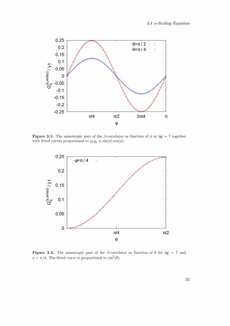
3.4 α-Scaling Equation
-0.25-0.2
-0.15-0.1
-0.05 0
0.05 0.1
0.15 0.2
0.25
π/4 π/2 3π/4 π
Gq(s
,ani
so) /
· γ t
φ
θ=π / 2θ=π / 4
Figure 3.1: The anisotropic part of the β-correlator as function of φ at |q| = 7 togetherwith fitted curves proportional to qxqy ∝ sin(φ) cos(φ).
0
0.05
0.1
0.15
0.2
0.25
π/4 π/2
Gq(s
,ani
so) /
· γ t
θ
φ=π / 4
Figure 3.2: The anisotropic part of the β-correlator as function of θ for |q| = 7 and
φ = π/4. The fitted curve is proportional to sin2(θ).
35

3 Incoherent Density Fluctuations
0.16
0.18
0.2
0.22
0.24
0.26
0 5 10 15 20
Gq(s
,ani
so) /
· γ t
q
θ=π/2, φ=π/4
Figure 3.3: Dependence of the anisotropic part of the β-correlator on the lengths q of thewavevector.
-2
-1.5
-1
-0.5
0
0.5
1
1.5
2
-2.5 -2 -1.5 -1 -0.5 0 0.5 1 1.5 2 2.5
y
x
Figure 3.4: Lines with constant single particle probability density P (r, r0 = 0, t = 1) =1/100, see Eq. (1.8). Without shear (solid line), the line forms a circle. With shear (dashedline), the circle is stretched. The dynamics is enhanced for some regions and reduced forothers. Dashed dotted line shows x = y.
36

3.5 Stationary Versus Transient Initial Decay Rate
The incoherent density correlator reaches a scaling function Φs+q (t) in this limit, with
t =√
c(γ)/(λ − 12)γt. To derive the equation for Φs+
q (t), we start with the convolution
integral in Eq. (3.38),∫ t
0ms
q(t, t′) ∂t′Φsq(t′). (3.49)
In Eq. (3.40), we saw explicitely the dependence1 of msq(t, t′),
msq(t, t′) = ms
q(γt′)(t − t′). (3.50)
It depends only on γt′ rather than on t′. It does so via the advected wavevector. Thatmeans that the dependence on t′ already obeys the yield scaling law. Using this, we canrewrite the integral in Eq. (3.49) to
−msq(t) +
d
dt
∫ t
0dt′ms
q(γt′)(t − t′)Φsq(t′)
−∫ t
0dt′
∂q(γt′)
∂t′·(
∂
∂q(γt′)ms
q(γt′)(t − t′)
)
Φsq(t′). (3.51)
We now see that the correlator for long times obeys the scaling equation (with γt =√
(λ − 12)/c(γ) t = ct),
Φs+q (t) = ms+
q (t) − d
dt
∫ t
0dt′ms+
q(ct′)(t − t′)Φs+
q (t′)
+
∫ t
0dt′
∂q(ct′)
∂t′·(
∂
∂q(ct′)ms+
q(ct′)(t − t′)
)
Φs+q (t′). (3.52)
This equation is difficult to solve because it contains the derivative of the correlator withrespect to wavevector, but it shows that the correlator indeed shows yield scaling if thememory function does not depend on t−t′ only. The reason is that the advected wavevec-tors causing the deviation from t− t′ naturally show yield scaling. Using Eqs. (3.45) and(1.30), we hence find at ε = 0,
Φs+q (t → 0) = f sc
q − hsq t, (3.53)
with hsq = hs
q(1 + G(q)c) with G(q) in Eq. (3.47). It can be straight forwardly shownthat (3.53) solves the α-scaling equation Eq. (3.52) for short times. This closes ourdiscussion of the dynamics of the incoherent density correlator.
3.5 Stationary Versus Transient Initial Decay Rate
Before turning to the mean squared displacements, let us briefly discuss a somewhatdifferent topic. In simulations of hard spheres under shear, it is unclear whether the
1q(γt) is equal to q(t) defined earlier. We apologize for this inconsistency.
37

3 Incoherent Density Fluctuations
initial decay rate of incoherent density fluctuations perpendicular to the shear directiondepends on shear rate [66]. This question can be answered by regarding the expressionsfor the initial decay rate in the stationary state for qx = 0,
Γ(s,γ)q = −
⟨
e−iq·rsΩ†eiq·rs
⟩(γ)= −
⟨
e−iq·rsΩ†eiq·rs
⟩
−γ
∫ ∞
0ds⟨
σxyeΩ†se−iq·rsΩ†eiq·rs
⟩
.
(3.54)The first term on the right hand side is equal to q2. The second one vanishes,
γ
∫ ∞
0ds⟨
σxyeΩ†se−iq·rsΩ†eiq·rs
⟩
= γ
∫ ∞
0ds⟨
σxyeΩ†s(−q2 + iq ·F)
⟩
= 0. (3.55)
The first term in the brackets is a constant and vanishes [60]. The second term containsFz and Fy. It can be rewritten to
γ
∫ ∞
0ds⟨
σxyeΩ†sFz/y
⟩
=⟨Fz/y
⟩(γ) −⟨Fz/y
⟩= 0. (3.56)
It is clear that the average value of the force on the tagged particle perpendicular to theflow must vanish in both averages, and the difference is hence zero as well. We concludethat the initial decay rate in the steady state is equal to the transient initial decay rate.The latter is equal to the one of the un-sheared system for qx = 0 and hence independentof shear rate,
Γ(s,γ)q = −
⟨
e−iq·rΩ†eiq·r⟩(γ)
= −⟨
e−iq·rΩ†eiq·r⟩
= q2. (3.57)
3.6 Mean Squared Displacements
In this section, we will derive equations for the mean squared displacement (MSD) of atagged particle for the different spatial directions and show their asymptotic solutionsfor long times. We will first rewrite the memory function ms
q(t, t′) into a product of thepart which depends only on the difference t − t′ and the part which depends explicitelyon t and t′,
msq(t, t′) =
∑
k
k(t − t′) · q(t)
q2(t)
k · q(t′)
q2(t′)F (k,q(t′), t − t′), (3.58)
where the function F depends still explicitely on t′ via the wavevector q(t′), see Eq. (3.39).However, this dependence will vanish in the low q limit as used for the calculation of theMSDs. Since the MSD will be anisotropic, as was already seen in the low density case,(1.9), we will discuss the different directions separately.
3.6.1 Neutral Direction
The calculation for the neutral direction is in strong analogy to the equilibrium case[77, 81]. We expand the correlator in qz to get
Φsqez
(t) = 1 − q2
2δz2(t) + O(q4), (3.59)
38

3.6 Mean Squared Displacements
where δz2(t) is the transient mean squared displacement of the particle in z-direction,corresponding to the average square of the traveled distance of the particle in simulationsor experiments. Its equation of motion is achieved by inserting (3.59) into (3.38) keepingonly the terms of order q2. The equation is then integrated over time to get,
− 1
2δz2(t) + t − 1
2
∫ t
0dt′∫ t′
0dt′′m0
z(t′ − t′′)∂t′′δz
2(t′′) = 0, (3.60)
with the memory function in the low q limit
m0z(t) =
∑
k
kzkz F (k,0, t). (3.61)
Since m0z(t) has only one time-argument, one can rewrite the above equation using the
standard trick of partial integrations and δz2(t = 0) = 0,
δz2(t) +
∫ t
0dt′m0
z(t − t′)δz2(t′) = 2t. (3.62)
Eq. (3.62) now looks similar to the equilibrium case [77]. The long time limit of thesolution corresponds to the small-z part of its Laplace transform δz2(z) =
∫∞0 e−z tδz2(t).
The convolution theorem can be applied. We find for t → ∞,
limt→∞
δz2(t) =2t
1 + m0z(z = 0)
. (3.63)
In contrast to the equilibrium case, m0z(z = 0) is always finite under shear, as we
saw in Sec. 3.3, and the MSD is always diffusive at long times. In the glass, we havelimγ→0 m0
z(z = 0) ∝ |γ|−1 (compare the α-scaling equation Eq. (3.52)) leading to thescaling relation at small shear rates,
limt→∞
δz2(t) = 2βz |γ|t, (3.64)
where the coefficient βz = (|γ|m0z(z = 0))−1 is asymptotically independent of shear rate.
We see that the long time diffusivity is then independent of the short time diffusivityD0.
3.6.2 Gradient Direction
The gradient direction is similar to the neutral direction, we only treat it separately herebecause the MSDs in flow-, i.e. in x-direction will be coupled to the one in y-direction.The correlator is expanded in qy,
Φsqey
(t) = 1 − q2
2δy2(t) + O(q4). (3.65)
The equation of motion for the MSD in gradient direction reads
δy2(t) +
∫ t
0dt′m0
y(t − t′)δy2(t′) = 2t, (3.66)
39

3 Incoherent Density Fluctuations
with the memory function
m0y(t) =
∑
k
ky(t)ky F (k,0, t). (3.67)
As expected, the long time limit of δy2(t) is given by
limt→∞
δy2(t) =2t
1 + m0y(z = 0)
. (3.68)
This leads to a scaling relation similar to Eq. (3.64) for glassy states at low shear rates,
limt→∞
δy2(t) = 2βy|γ|t. (3.69)
We have no reason to expect that the coefficients βy and βz are equal. These have beenfound slightly different in simulations [65, 82].
3.6.3 Flow Direction
The derivation of the MSD in flow direction is more involved. We first have to identifythe term that describes the average squared distance of the particle to its position att = 0 measured in experiments or simulations. The connection of the density correlatorfor q = qex to measured quantities is a general nontrivial question. Let us recall thetranslational invariant correlator for the x-direction
Φsqex
(t) =⟨
e−iqxseΩ†teiqxse−γtiqys
⟩
. (3.70)
In the small density limit, the quantity δx2(t), measured in experiments as the averagevalue of (x(t) − x(0))2 follows from taking the q → 0-limit of Φs
qex(t), as we will see
below. We hence conclude that this holds also at higher densities and write
Φsqex
(t) = 1 − 1
2q2δx2(t) + O(q4). (3.71)
The equation for δx2(t) is gained by expanding the equation for the correlator Φsq(t) in
qx and by integrating with respect to t,
δx2(t) +
∫ t
0dt′∫ t′
0dt′′∑
k
(kx − γt′ky(t
′ − t′′)) kx − γt′′ky
1 + (γt′′)2F (k,0, t′ − t′′)∂t′′δx
2(t′′)
= 2
∫ t
0dt′
Γsqex
(t′)
q2. (3.72)
As promised, we would like to consider the low density limit before we start analyzingthis equation. In this limit, the memory function vanishes, and we have
δx2(t) = 2
∫ t
0dt′
Γsqex
(t′)
q2= 2t +
2
3γ2t3, (3.73)
40

3.6 Mean Squared Displacements
i.e., we recover the low density limit of Eq. (1.9) without the term proportional to y20.
This is due to the fact the we consider translational invariant terms and the calculatedexpectation values cannot depend on initial conditions.
The memory function in Eq. (3.72) is not a function of the difference of its argumentsonly and we cannot use the convolution theorem. It is nevertheless still possible todetermine the leading long time behavior, in which we are interested here. For this wewrite
limt→∞
δx2(t) = at3 + bt2 + ct + . . . . (3.74)
The form (3.74) can be justified knowing that the function F in Eq. (3.72) always decaysto zero. A term t4 (or higher powers in t, or fractional powers) does not exist since theinitial decay rate does not contain such a term. The long time behavior is hence governedby the initial decay rate, a fact which is interesting because the long time behavior ofthe correlator Φs
q(t) is independent of the initial decay rate, see the α-scaling equation(3.52). This is due to the fact that the limits of t → ∞ and q → 0 do not commute.
We first determine the coefficient a. For this, the leading long time (large t′ and t′′)terms in the double integral are needed which are independent of the coefficient b. Theequation for b, on the other hand, will contain the coefficient a and can hence only besolved afterwards. The leading term of the first bracket is −γt′ky(t
′ − t′′), the leadingterm of the fraction is given by −ky/(γt′′). With this, we get
at3 +
∫ t
0dt′∫ t′
0dt′′γt′m0
y(t′ − t′′)
∂t′′at′′3
γt′′=
2γ2
3t3. (3.75)
We note that m0y(t) appears. This equation can be treated with the following formulae
for Laplace transforms [83],
L∫ t
0dt′f(t′)
(z) =1
zLf(t) (z), (3.76a)
Ltf(t) (z) = − ∂
∂zLf(t) (z). (3.76b)
Using this, we find that the two integrals in the expression above contain also one termof order t2 (because ∂zm
0y(z) is finite as z → 0), which is neglected in this order. We
find
a =2γ2
3 + 3m0y(z = 0)
. (3.77)
Let us celebrate: We found the Taylor dispersion for Brownian particles at the glasstransition. The intriguing result is that the coefficient for the t3 term is connected tothe long time diffusion coefficient in y-direction in the same way as in the low densitylimit. We can write
δx2(t) =2
3δy2(t)γ2t2 + O(t2), (3.78)
which holds identically in the low density limit, Eq. (1.9), and was also found in Ref. [68]for non-Brownian particles, see Sec. 3.1. We see that this relation comes about because
41

3 Incoherent Density Fluctuations
the long time terms in the memory function in Eq. (3.75) are given by the memoryfunction for the y-direction. This is physically very plausible if we recall the reason forthe t3-term: If the particle diffuses in y-direction, it gets a “boost” in x-direction due tothe shear flow. It is hence not surprising that the t3 term is proportional to δy2(t), butthe result that the very same relation holds as in the low density limit is nontrivial andunexpected. Another interesting point is that we find a new type of Taylor dispersionin the glass at small shear rates. It is in contrast to the low density limit independentof the bare diffusivity D0 (set to unity here) and obeys the yield scaling law,
δx2(t) =2
3βy γ
2|γ|t3 + O(t2), (3.79)
with the same βy as in Eq. (3.69). This is in agreement to recent simulations [65, 66].We should not forget to consider the next order leading term. We will need this term
later in order to calculate the xy cross correlation. For the equation for the coefficientb, we have to collect all terms proportional to t2 at long times, (note that some of thepossible contributions vanish in the sum over k due to symmetries2),
2b + 2bm0y(z = 0) − 3a∂zm
0y(z = 0) − 3a
m0xy(z = 0)
γ= 0. (3.80)
The promised dependence of b on a appears. Also, the diagonal memory function enters,
m0xy(t) =
∑
k
ky(t)kx F (k,0, t). (3.81)
We find for b,
b =3a
2
(∂zm
0y(z = 0)
)+
m0xy(z=0)
γ
1 + m0y(z = 0)
. (3.82)
We found a term proportional to t2, which is not present in the low density limit. Itcomes about because the memory function is not a function of t− t′. The actual value ofthe pre-factor b has to be determined in full microscopic calculations. We also want torecall that we are currently calculating the transient MSD. The stationary MSD mightnot have a term of order t2 even if the transient has one.
3.6.4 Cross Correlation
In the system under shear, there is a correlation between x and y which is not presentwithout shear, see Eq. (1.9). In order to calculate this, we go to the small q limit for thedirection
q(t = 0) =
qq0
. (3.83)
2Although the memory function including the correlators is not isotropic under shear, it is still sym-metric with respect to the origin, k = 0, since the system is symmetric with respect to the origin.
42
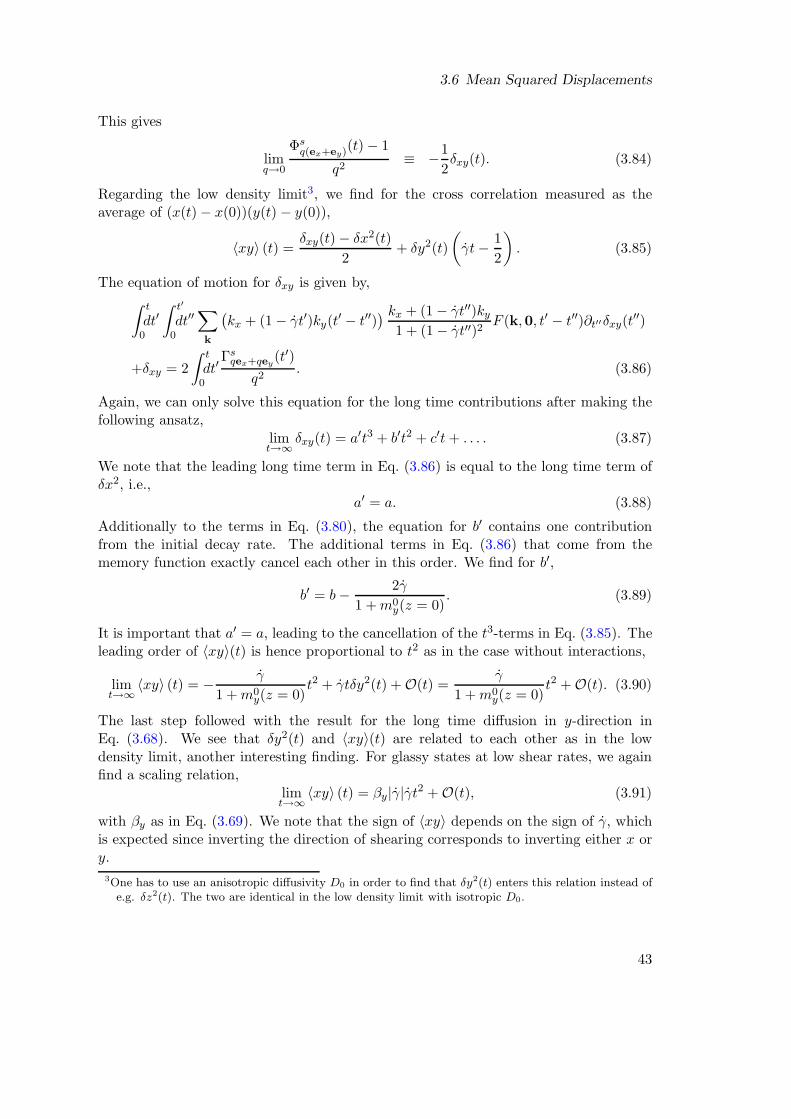
3.6 Mean Squared Displacements
This gives
limq→0
Φsq(ex+ey)(t) − 1
q2≡ −1
2δxy(t). (3.84)
Regarding the low density limit3, we find for the cross correlation measured as theaverage of (x(t) − x(0))(y(t) − y(0)),
〈xy〉 (t) =δxy(t) − δx2(t)
2+ δy2(t)
(
γt − 1
2
)
. (3.85)
The equation of motion for δxy is given by,
∫ t
0dt′∫ t′
0dt′′∑
k
(kx + (1 − γt′)ky(t
′ − t′′)) kx + (1 − γt′′)ky
1 + (1 − γt′′)2F (k,0, t′ − t′′)∂t′′δxy(t
′′)
+δxy = 2
∫ t
0dt′
Γsqex+qey
(t′)
q2. (3.86)
Again, we can only solve this equation for the long time contributions after making thefollowing ansatz,
limt→∞
δxy(t) = a′t3 + b′t2 + c′t + . . . . (3.87)
We note that the leading long time term in Eq. (3.86) is equal to the long time term ofδx2, i.e.,
a′ = a. (3.88)
Additionally to the terms in Eq. (3.80), the equation for b′ contains one contributionfrom the initial decay rate. The additional terms in Eq. (3.86) that come from thememory function exactly cancel each other in this order. We find for b′,
b′ = b − 2γ
1 + m0y(z = 0)
. (3.89)
It is important that a′ = a, leading to the cancellation of the t3-terms in Eq. (3.85). Theleading order of 〈xy〉(t) is hence proportional to t2 as in the case without interactions,
limt→∞
〈xy〉 (t) = − γ
1 + m0y(z = 0)
t2 + γtδy2(t) + O(t) =γ
1 + m0y(z = 0)
t2 + O(t). (3.90)
The last step followed with the result for the long time diffusion in y-direction inEq. (3.68). We see that δy2(t) and 〈xy〉(t) are related to each other as in the lowdensity limit, another interesting finding. For glassy states at low shear rates, we againfind a scaling relation,
limt→∞
〈xy〉 (t) = βy|γ|γt2 + O(t), (3.91)
with βy as in Eq. (3.69). We note that the sign of 〈xy〉 depends on the sign of γ, whichis expected since inverting the direction of shearing corresponds to inverting either x ory.
3One has to use an anisotropic diffusivity D0 in order to find that δy2(t) enters this relation instead ofe.g. δz2(t). The two are identical in the low density limit with isotropic D0.
43

3 Incoherent Density Fluctuations
3.7 Schematic Models
In order to illustrate the results we gained in the previous sections of this chapter, weintroduce a schematic model for the incoherent transient density correlator Φs
q(t), wherethe q dependence is dropped. We will therefore advance the so called Sjogren model [84]for the incoherent transient density correlator without shear and afterwards introduceschematic equations for the MSDs.
3.7.1 (γ)-Sjogren Model
The equation of motion for Φs(t) in the (γ)-Sjogren model reads
Φs(t) + Γ
Φs(t) +
∫ t
0dt′ms(γ, t − t′)Φs(t′)
= 0. (3.92)
The memory function is approximated in analogy to (3.39) and (1.41),
ms(γ, t) =1
1 + (γt/γsc )
2vsΦ
s(t)Φ(t). (3.93)
The original Sjogren model is given with ms(0, t). The additional advection of thevertex in (3.39) is modeled by the shear dependent pre-factor. The coupling of thetagged particle to the surrounding particles is represented by the parameter vs. One canshow that the non-ergodicity parameter f s of Φs(t) is connected to the parameter of thecoherent correlator by
f s = 1 − 1
vsf. (3.94)
For vs < 1/f , the incoherent correlator is decoupled from the coherent one, correspondingto the percolation threshold discussed above. The tagged particle is then small enoughto move through the glassy matrix of host particles. For the standard values vc
1 and vc2
used in the F(γ)12 -model, this threshold value for vs is roughly vs = 3.4 at ε = 0. We will
use4 vs = 5. The parameter γsc plays a role analogous to γc in Eq. (1.41), i.e., it tunes
the strain γt, at which the cages break. Again, see Refs. [53, 55, 56] for the numerical
algorithm to solve Eq. (3.92), which is similar to the one for the F(γ)12 -model. Fig. 3.5
shows Φs together with Φ for a glassy state and γsc = 1. We see that the final decay of
the incoherent correlator is faster than the decay of the coherent correlator due to theadditional advection in the incoherent vertex.
3.7.2 Mean Squared Displacements
For the MSDs, we use the simplest possible equations that contain our findings of Sec. 3.6.They will be isotropic in the plane perpendicular to the flow and ez shall denote any
4This value is rather small compared to studies of the original Sjogren model [63], but the author foundthe final shear induced relaxation to get slower with increasing values of vs making smaller values ofγs
c necessary to observe the linear part in the MSD in Sec. 3.7.2.
44

3.7 Schematic Models
0
0.1
0.2
0.3
0.4
0.5
0.6
0.7
0.8
0 1 2 3 4 5 6 7 8 9
Φ
log10 Γ t
ΦΦs
Figure 3.5: Transient coherent and incoherent correlators from the F(γ)12 -model and the
(γ)-Sjogren model for a glassy state (ε = 10−3) at shear rates of γ/Γ = 10−8, 10−6, 10−4,10−2 from right to left. Lines on the right hand side mark the non-ergodicity parameters.
direction in the yz-plane. The schematic equation reads (compare Eq. (3.62)),
δz2(t) +
∫ t
0ms(t − t′)δz2(t) = 2t, (3.95)
where the memory function ms(t− t′) is given in Eq. (3.93). In the microscopic equation(3.62) the limit of q → 0 of the memory function appears. This limit cannot be performedin the schematic model and there is no reason to introduce a difference between thememory function at q → 0 and at finite q. From Eq. (3.95), the diffusive long time limitof the MSD in z-direction follows directly,
limt→∞
δz2(t) =2t
1 + ms(z = 0). (3.96)
For the x-direction, we use a schematic version of Eq. (3.72), which can be simplifiedbecause ms(t, t′) = ms(t − t′),
δx2(t) +
∫ t
0ms(t − t′)δx2(t) = 2t +
2
3γ2t3. (3.97)
The long time limit follows,
limt→∞
δx2(t) =2t + 2
3 γ2t3
1 + ms(z = 0), (3.98)
45

3 Incoherent Density Fluctuations
-1
0
1
2
3
4
5
6
5.5 6 6.5 7 7.5 8 8.5 9 9.5
log 1
0 <(
r(t)-
r)2 >
log10 Γ t
x - direction−z - direction
Figure 3.6: The MSD in flow direction and perpendicular for γ/Γ = 10−8 and ε = 10−3.
γsc−2 = 10n with n = 0, . . . , 5 from right to left. The dotted curves show the long time
behavior according to Eq. (3.98).
i.e., b = 0 in Eq. (3.74), in contrast to the microscopic calculation. We already stressed inSec. 3.6.3 that b 6= 0 appears due to the two arguments t and t′ of the memory function.See again Refs. [53, 55] for the numerical algorithm to solve Eqs. (3.95) and (3.97).While in all our calculations concerning coherent quantities, the parameter γc can bescaled out, the parameter γs
c cannot be scaled out concerning the MSDs. This is due tothe fact that a new timescale, namely γ−1, enters via the initial decay rate in x-directionin Eq. (3.97). Fig 3.6 shows the MSDs for different values of γs
c at γ/Γ = 10−8 andε = 10−3. For γs
c = 1, the dynamics of the system is slow compared to the initial decayrate, and the term proportional to t in Eq. (3.98) cannot be observed. For smaller valuesof γs
c , the linear term becomes more and more pronounced. In the following, we willuse the value of γs
c = 1/10, as was done in Ref. [13] for the coherent case. In Fig. (3.7)we show the MSDs for different shear rates for a glassy state. The different shear rateslook qualitatively similar, we observe the diffusive behavior for the z-direction and theTaylor behavior for the x-direction. In Fig. 3.8, the curves are shown as function ofstrain γt, where the yield scaling of Eq. (3.69) and (3.79) is observed, i.e., for γ → 0,the curves fall on top of each other. The liquid case is of interest also, as shown inFig. 3.9. At small shear rates, the MSD perpendicular to the shear direction becomesindistinguishable from the γ = 0 case. But the Taylor dispersion is still present, i.e., theMSD in x-direction still shows a term t3 at long times. Only the pre-factor shows noyield scaling any more, i.e, ms(z = 0) in Eq. (3.98) becomes independent of shear rate.
46

3.7 Schematic Models
-0.5
0 0.5
1 1.5
2 2.5
3 3.5
4
0 1 2 3 4 5 6 7 8 9
log 1
0 <(
r(t)-
r)2 >
log10 Γ t
x - direction−z - direction
Figure 3.7: The MSD in flow direction and perpendicular for ε = 10−3 and γsc = 1/10.
Shear rates are γ/Γ = 10−8,−6,−4,−2 from right to left. The dotted curves show the longtime behavior according to Eq. (3.98).
-0.5 0
0.5 1
1.5 2
2.5 3
3.5 4
4.5
-2 -1.5 -1 -0.5 0 0.5 1
log 1
0 <(
r(t)-
r)2 >
log10 •γ t
•γ / Γ = 10-8
= 10-6
= 10-4
= 10-2
Figure 3.8: The MSD in flow direction and perpendicular for ε = 10−3 and γsc = 1/10 as
function of strain γt. For γ → 0, the long time part of the curves fall on top of each other.
47

3 Incoherent Density Fluctuations
-2
0
2
4
6
8
10
0 2 4 6 8 10 12
log 1
0 <(
r(t)-
r)2 >
log10 Γ t
x - direction−z - direction
Figure 3.9: The MSD in flow direction and perpendicular for ε = −10−3 (fluid). Shearrates are γ/Γ = 10−10,−8,−6,−4,−2 from right to left. The dotted curves show the long timebehavior according to Eq. (3.98).
We note that the MSD in x-direction is an example for a quantity which can distinguishthe shear from the no shear case even in the fluid at low shear rates.
3.8 Stationary Mean Squared Displacements
Let us recall that we so far calculated the transient mean squared displacements, i.e.,γ = 0 for t < 0 and γ 6= 0 for t ≥ 0. Before we discuss the difference between these andthe stationary ones, let us emphasize their commonality: A very long time after switch-on of the rheometer the time derivative of the transient MSD must reach the timederivative of the corresponding stationary MSD. This is true because at these very longtimes the transient correlator describes the stationary state and the long time diffusivitymust be the one of the steady state. All the results for the respective leading order (∝ tperpendicular and ∝ t3 parallel to the flow) we achieved in the previous section are validfor the stationary MSDs as well, with the same pre-factors. Our ITT approach of firstderiving the transient quantities and then deriving the stationary ones from them, provesto be a simplification and advantage here: For the long time diffusivity, the second stepis not necessary, it follows directly from the equation for the transient MSD.
Nevertheless, at intermediate times, there is a difference, as measured in Ref. [14]. Inthe following, the notation δ(γ)z2(t) and δ(e)z2(t) for stationary and equilibrium MSDswill be used to distinguish them from the transient ones. The stationary MSD can easily
48

3.8 Stationary Mean Squared Displacements
be derived via Eq. (2.19) for the respective correlator. At t = 0 the MSDs are triviallyzero, i.e., the first term in (2.19) vanishes. For the directions perpendicular to the flow(again denoted z), we find
δ(γ)z2(t) ≈ δz2(t) − 2σ
γlimq→0
Φsqez
(t) − Φs(e)qez (t)
Φsqez
(t)
Φs(e)qez (t)
q2. (3.99)
The limit q → 0 is easily performed since the derivatives are of order q2 and the q = 0
value of the fraction Φsqez
(t)/Φ(s,e)qez (t) is equal to unity,
δ(γ)z2(t) ≈ δz2(t) +σ
γ∂t
(
δz2(t) − δ(e)z2(t))
. (3.100)
From Eq. (3.100) we have that the stationary MSD is larger than the transient oneif δz2(t) is larger than δ(e)z2(t), which is expected and observed in experiments andsimulations. It cannot be shown rigorously.
Using the schematic model in Eq. (3.95) and the normalized stress σ from Eq. (2.7),we can visualize the two different MSDs. We want to emphasize that we use γs
c = 1,because otherwise the modulus, as approximated in Eq. (3.100), would relax too slowlycompared to the memory function ms(t), giving a too large σ. Another option wouldbe to use γs
c = 1/10 and γc = 1/10 in Eq. (1.40), i.e., we need γsc = γc here. In
Fig. 3.10 we show the result for a glassy state and different shear rates. The discussedrelation is observed. Fig. 3.10 is in excellent qualitative agreement to the simulationsand experiments reported in Ref. [14]. The transient MSD follows the quiescent oneuntil γt/γs
c ≈ 0.1 and joins the steady one at γt/γsc ≈ 1, which is also in good agreement
with the simulations and experiments. A last comment; in the simulations and, lesspronounced, also in the experiments in Ref. [14], the transient MSD is super-diffusivefor intermediate times. This behavior is connected to the overshoot of the transientshear stress. Such a behavior can only result from Eq. (3.95) if ms(t) is negative forintermediate times and needs further theoretical studies. The stress overshoot is notcontained in the schematic model by construction.
49

3 Incoherent Density Fluctuations
-0.4-0.2
0 0.2 0.4 0.6 0.8
1 1.2 1.4
0 1 2 3 4 5 6 7 8 9
log 1
0 <(
r(t)-
r)2 >
log10 Γ t
quiescenttransient
stationary
Figure 3.10: Quiescent, transient and stationary MSDs perpendicular to the flow directionin the schematic model for ε = 10−3 (glass) and γs
c = 1. Shear rates are γ/Γ = 10−8,−6,−4,−2
from right to left.
50

4 Fluctuation Dissipation Relations underSteady Shear
In this chapter, we study the fluctuation dissipation theorem (FDT) [22, 85] under shear.This was the focus of study of the author during the last three years and was motivatedby the findings in the simulations in Ref. [1] and the interpretation of these findings interms of an effective temperature. After the introduction, Secs. 4.1–4.4, this chapter willbe split into two parts. First, we will in Sec. 4.5 show a treatment of the new terms inthe FDT within the Zwanzig-Mori projection operator formalism. In Sec. 4.6 we willshow the connection of one of the new terms to the waiting time derivative discussed inChap. 2, which will lead to interesting and special predictions. In both approaches wefind the same qualitative features of the FDT under shear, namely the response functionis smaller at long times as estimated by the equilibrium FDT and the ratio betweenresponse and fluctuation functions is nearly constant in time. The reader primarilyinterested in the final results and opinion of the author may want to skip Sec. 4.5. Thereader who wants to see that the results presented in Sec. 4.6 are backed by a detailedanalysis within MCT is referred to Sec. 4.5.
4.1 Fluctuation Dissipation Theorem (FDT) and – Ratio(FDR)
In thermal equilibrium, the response of a system to a small external force follows directlyfrom thermal fluctuations of the unperturbed system. This connection is the essence ofthe fluctuation dissipation theorem (FDT) which lies at the heart of linear response
theory. In our framework, the FDT in equilibrium connects the correlator C(e)fg (t) with
the response function, the susceptibility χ(e)fg (t) (defined below), and reads with restored
units
χ(e)fg (t) =
−1
kBT
∂
∂tC
(e)fg (t). (4.1)
Eq. (4.1) will be proven when deriving the microscopic form of the susceptibility forSmoluchowski dynamics in Sec. 4.3. It states that the relaxation of a small fluctuation isindependent of the origin of this fluctuation: Whether induced by a small external forceor developed spontaneously by thermal fluctuations, the relaxation cannot distinguishthese cases.
The most famous example for the FDT is given by the Einstein relation for the diffu-sivity of a free Brownian particle. One can consider two experiments, see Fig. 4.1: First,we watch the particle perform the random walk and measure the average mean squared
51
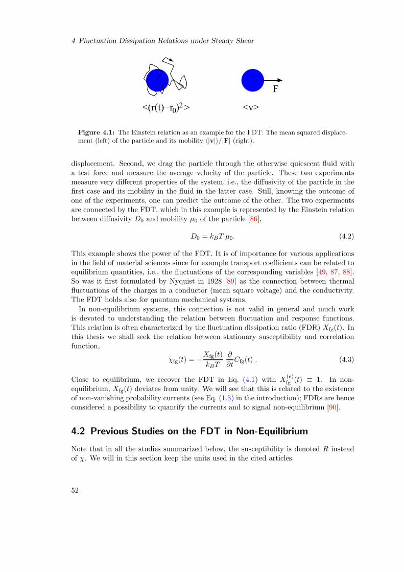
4 Fluctuation Dissipation Relations under Steady Shear
F
<v><(r(t)−r )2 >0
Figure 4.1: The Einstein relation as an example for the FDT: The mean squared displace-ment (left) of the particle and its mobility 〈|v|〉/|F| (right).
displacement. Second, we drag the particle through the otherwise quiescent fluid witha test force and measure the average velocity of the particle. These two experimentsmeasure very different properties of the system, i.e., the diffusivity of the particle in thefirst case and its mobility in the fluid in the latter case. Still, knowing the outcome ofone of the experiments, one can predict the outcome of the other. The two experimentsare connected by the FDT, which in this example is represented by the Einstein relationbetween diffusivity D0 and mobility µ0 of the particle [86],
D0 = kBT µ0. (4.2)
This example shows the power of the FDT. It is of importance for various applicationsin the field of material sciences since for example transport coefficients can be related toequilibrium quantities, i.e., the fluctuations of the corresponding variables [49, 87, 88].So was it first formulated by Nyquist in 1928 [89] as the connection between thermalfluctuations of the charges in a conductor (mean square voltage) and the conductivity.The FDT holds also for quantum mechanical systems.
In non-equilibrium systems, this connection is not valid in general and much workis devoted to understanding the relation between fluctuation and response functions.This relation is often characterized by the fluctuation dissipation ratio (FDR) Xfg(t). Inthis thesis we shall seek the relation between stationary susceptibility and correlationfunction,
χfg(t) = −Xfg(t)
kBT
∂
∂tCfg(t) . (4.3)
Close to equilibrium, we recover the FDT in Eq. (4.1) with X(e)fg (t) ≡ 1. In non-
equilibrium, Xfg(t) deviates from unity. We will see that this is related to the existenceof non-vanishing probability currents (see Eq. (1.5) in the introduction); FDRs are henceconsidered a possibility to quantify the currents and to signal non-equilibrium [90].
4.2 Previous Studies on the FDT in Non-Equilibrium
Note that in all the studies summarized below, the susceptibility is denoted R insteadof χ. We will in this section keep the units used in the cited articles.
52

4.2 Previous Studies on the FDT in Non-Equilibrium
4.2.1 The General Formula for the Susceptibility in Non-Equilibrium
The general linear response susceptibility for non-equilibrium states with Fokker-Planckdynamics [22] has been derived by Agarwal in 1972 [91]. It is Eq. (4.28) for our Smolu-chowski dynamics, which will be the starting point of our analysis. The susceptibility isgiven in terms of microscopic quantities, which cannot be identified with a measurablequantity in general in contrast to the equilibrium case.
4.2.2 FDT Violation for a Single Driven Particle
For a single driven Brownian particle in a periodic potential, the FDT violation for thevelocity correlation has been studied in Ref. [92]. The susceptibility for fluctuations ofthe velocity x of the particle is defined as
Rx(t − τ) =δ〈x(t)〉pδfp(τ)
∣∣∣∣fp=0
, (4.4)
where 〈. . . 〉p denotes the average under the probe force fp on the particle. They find
TRx(t − τ) = 〈x(t)x(τ)〉 − 〈x(t)vs(x(τ))〉, (4.5)
where 〈. . . 〉 is the average in the unperturbed driven system. The last term in Eq. (4.5)is the term violating the equilibrium FDT. vs(x) is the local mean velocity at positionx given by the probability current corresponding to Ψ−1
s jsi in Eq. (1.5). It is found thatthe equilibrium FDT is restored if the velocity fluctuations are measured with respectto vs(x), i.e. for v(t) = x(t) − vs(x(t)),
TRv(t − τ) = 〈v(t)v(τ)〉. (4.6)
The local mean velocity depends on the position of the particle in the potential. Wewill come back to this in Chap. 5. These derivations have successfully been comparedto the experimental realization of the system [93]. The authors achieved to measure thediffusivity, the mobility and the theoretical expressions for the violating term separatelyto show that the derived expressions hold.
4.2.3 FDT Violation in Spin Glasses – Effective Temperature
We want to briefly summarize the violation of the equilibrium FDT as derived in spin-glass calculations following Ref. [94]. A so called p-spin model is considered with Hamil-tonian containing the interactions,
H =∑
j1<···<jp
Jji...jp si . . . sjp. (4.7)
J is the coupling between the continuous variables si. The Langevin equations for thespins si read,
∂si(t)
∂t= −µ(t)si(t) −
δH
δsi(t)+ fdrive
i (t) + ηi(t). (4.8)
53

4 Fluctuation Dissipation Relations under Steady Shear
They contain the damping µ(t), the external drive (corresponding to the shear) fdrivei (t)
and a Gaussian noise term ηi(t). The equations are coupled via the Hamiltonian. Inelaborate approximation steps, which are known to hold for “mean field like” systems,the above equation is then written as two coupled equations for the correlation C(t, t′) =∑
i〈si(t)si(t′)〉 and the response R(t, t′) =
∑
i〈δsi(t)/δηi(t′)〉.
Without external drive, the system shows a transition from equilibrium above Tc
to an aging system below Tc. With external drive, time translational invariance andergodicity are recovered. For small external driving, the solutions for R and C are thensplit into a short time and a long time contribution. While the short time contributionsare connected by the equilibrium FDT, the slow parts are found to be related as
Rs(τ) = − 1
Teff
dCs(τ)
dτ. (4.9)
The equilibrium form of the FDT is restored with pre-factor 1/Teff instead of 1/T . Thevalue of Teff is found to agree with the one of the corresponding calculation for the agingsystem. We note that in the initial equations of motion, the susceptibility is coupled tothe correlation function, i.e., as far as the author can judge, one can only solve for bothfunctions simultaneously. This introduces the susceptibility in a natural way in contrastto the mode coupling theory for colloidal systems, where the correlation function isderived without knowing the susceptibility. It remains questionable, whether the meanfield closure leaves enough freedom for relations between R and C different from thesimple one in Eq. (4.9). While the prediction in Eq. (4.9) deserves appreciation, we willshortly summarize why the study of the FDT for sheared colloidal suspensions is stillnecessary.
The presented approach (MCT-ITT) for dense colloidal suspensions under shear is veryspecific to the system under consideration, the sheared fluid. It starts from microscopicexpressions containing the actual particle positions as functions of space and time, andthe external shear is implemented with its geometric specialties in contrast to Eq. (4.8).The derived observables are directly related to quantities measured in experiments andsimulations. As a consequence, specific properties of different observables can be derived,MCT-ITT predicts e.g. a yield stress which is not contained in the spin glass approach.The non-equilibrium FDT can hence also be studied for different observables, measuredin simulations, and possible differences for different variables can be detected, as willbe shown. Also, the general exact expression for the susceptibility connects it to theprobability current, thereby giving deeper insight into the nature of the FDT violation.
4.2.4 Universal FDRs X = 12
in Spin Models
Interesting universal FDRs were found in different spin models under coarsening [95–99]and under shear [100], where, at the critical temperature, a universal value of X = 1
2(with corrections [101]) in the long time limit was found. Since we will also find a value ofthe long time FDR close to 1
2 , we want to exemplary consider the derivation in Ref. [95]more closely. Considered is the ferromagnetic Ising chain with Glauber dynamics [102].
54

4.2 Previous Studies on the FDT in Non-Equilibrium
The Hamiltonian for the spins σn = ±1 reads
H = −J∑
n
σnσn+1. (4.10)
The Glauber dynamics consists of picking at every time step δt = 1/N a site i at randomand updating its spin according to the stochastic rule
σn(t) →
+1 with probability 1+tanh(hn(t)/kBT )2 ,
−1 with probability 1−tanh(hn(t)/kBT )2 .
(4.11)
The update probability for the spin depends on the two neighboring sites,
hn(t) = J(σn−1(t) + σn+1(t)). (4.12)
For high temperatures, the updated spin is random, whereas for low temperatures, itstrongly follows its neighbors. Starting from a random initial condition and quenchingthe system to a low temperature, the system relaxes to its paramagnetic equilibrium. Therelaxation time τeq diverges exponentially as approaching T = 0, the critical temperatureof the system. At T = 0, the updated spin will take the value of its neighbors if theseare equal and will be updated randomly if these are different. Domains of positive andnegative spins grow forever. Generally, one observes an aging regime for τ ∼ tw ≪ τeq
with t = τ + tw the correlation time and tw the waiting time, both measured after thequench. The two-time autocorrelation function is introduced as
C(t, tw) = 〈σn(t)σn(tw)〉. (4.13)
Due to translational invariance, it does not depend on n. The susceptibility R is givenas the change of the average of spin n with external field Hn(t) entering the local fieldin Eq. (4.12),
hn(t) = J(σn−1(t) + σn+1(t)) + Hn(t). (4.14)
R follows as
R(t, tw) = Tδ〈σn(t)〉δHn(tw)
∣∣∣∣H=0
. (4.15)
The fluctuation dissipation ratio is defined as
X(t, s) =R(t, tw)
∂C(t, tw)/∂tw. (4.16)
Interestingly, one uses the derivative with respect to waiting time. For time transla-tionally invariant states, one has C(t, tw) = C(t− tw) and the derivative with respect towaiting time is equal to minus the time derivative. Eq. (4.3) follows. In the regime whereall times are large, τ ∼ tw ∼ τeq ≫ 1, one finds the FDR in closed form (τeq = 2/µ2),
X(tw + τ, tw) =e−µ2tw + µ
√πtw erf(µ
√tw)
[2(tw + τ)/(2tw + τ)]e−µ2tw + µ√
πtwerf(µ√
tw). (4.17)
55

4 Fluctuation Dissipation Relations under Steady Shear
There are many time regimes with different values of the FDR between unity and 12 . In
the aging regime 1 ≪ tw ≪ τeq, the FDR for long times τ ≫ tw approaches the limitingvalue of
X∞ =1
2. (4.18)
At T = 0 this value holds for arbitrarily large waiting times tw. Unfortunately, it is notapparent from the derivation why the FDR takes this special value.
4.2.5 Simulation Results for the FDR under Shear and Further Works
As presented in Chap. 1, colloidal dispersions exhibit slow cooperative dynamics athigh concentrations and can arrest into metastable soft solids (glasses). Recall thatwhen putting these glassy states under shear, the final decay of the correlation fromthe plateau to zero is governed solely by shear, however small the shear rate. In thesestates, a very unexpected ‘restoration’ of the equilibrium FDT was found in computersimulations by Berthier and Barrat [1, 103, 104], which initiated the presented studies:During the final shear governed decay, the FDR measured in the vorticity direction, i.e.,the z-direction in our coordinate system, is different from unity, but constant in time.This ratio was also found to be independent of observable, which lead to the notion ofan effective temperature Xf = T/Teff describing the non-equilibrium state. The findingsare summarized by
χf(t) =
−1
kBT∂∂t Cf(t) short times,
−1kBTeff
∂∂t Cf(t) long times.
(4.19)
The corresponding spin glass calculations have been discussed in Sec. 4.2.3. Teff wasfound to be larger than the real temperature, which translates into an FDR smallerthan unity. Further simulations with shear also saw Teff > T [105–108], but the variabledependence was not studied in as much detail as in Ref. [1], and partially other definitionsof Teff were used. As mentioned in Sec. 4.2.3, it is argued in Refs. [1, 94, 109] that Teff inEq. (4.19) agrees with the effective temperature connected with the FDT violation in thecorresponding aging system [110, 111]. This has not yet been demonstrated for differenttemperatures. The fluctuation dissipation relation of aging systems using MCT wasinvestigated in Ref. [112]. Recently Teff was also connected to barrier crossing rates [113]replacing the real temperature in Kramers escape problem [22]. A theoretical approachfor the effective temperature under shear in the so called “shear-transformation-zone”(STZ) model is proposed in Ref. [114]. Different techniques (with different findings) tomeasure FDRs in aging colloidal glasses were used in Refs. [115–117]. No experimentalrealization of an FDT study of colloidal suspensions under shear is known to the author.An overview over the research situation (in 2003) can be found in Ref. [90].
4.3 Linear Response and Susceptibility
As pointed out in the example of the Einstein relation, the susceptibility describes theresponse of the system to an external perturbation. We will consider susceptibilities
56

4.3 Linear Response and Susceptibility
in the stationary state, i.e., the external steady shear flow was turned on a very longtime ago. The force necessary to shear the system is finite, see Sec. 1.6.4, i.e., the term‘linear response’ does not correspond to the shear, but to the small test force he(t)acting on the particles. It tests their linear response. Because the system is alwaysergodic due to shearing, the linear response will always exist in contrast to un-shearedglasses [118, 119], where a finite force is needed to mobilize the particles. Formally, thesusceptibility χfg(t) describes the linear response of the stationary expectation value ofg to the external perturbation he(t) shifting the internal energy U to U − f∗ he(t). Inthe following we will use dimensionless units again,
〈g〉(γ,he) (t) − 〈g〉(γ) =
∫ t
−∞dt′χfg(t − t′)he(t
′) + O(h2e) . (4.20)
Note that the definition above is equivalent to the definitions used in the articles sum-marized in Sec. 4.2, we can also write
χfg(t − t′) =δ 〈g〉(γ,he) (t)
δhe(t′)
∣∣∣∣∣he=0
. (4.21)
To derive the microscopic form of the susceptibility, we consider the change of the sta-tionary distribution function Ψs under the external perturbation. The SO changes toΩ − ∆Ω(Γ, t) with [21] (recall Γ = ri)
∆Ω(Γ, t) =∑
i
∂i ·(
∂
∂rif∗(Γ)
)
he(t). (4.22)
The linear change of Ψs due to the external force is then
Ψ(t) = Ψs + ∆Ψ(t) + O(h2e). (4.23)
With this, we can linearize the Smoluchowski equation,
∂
∂t(Ψs + ∆Ψ(t)) = (Ω − ∆Ω(t))(Ψs + ∆Ψ(t)) + O(h2
e). (4.24)
Using ∂∂tΨs = ΩΨs = 0, we have
∂
∂t∆Ψ(t) = Ω∆Ψ(t)− ∆Ω(t)Ψs + O(h2
e). (4.25)
Eq. (4.25) can be viewed as a homogeneous equation for ∆Ψ(t) with inhomogeneity∆Ω(t)Ψs. The solution for Ψ(t) is given by [91]
Ψ(t) = Ψs −∫ t
−∞dt′eΩ(t−t′)∆Ω(t′)Ψs + O(h2
e). (4.26)
Calculating the difference of the expectation values,
〈g〉(γ,he) (t) − 〈g〉(γ) =
∫
dΓΨ(t)g −∫
dΓΨsg, (4.27)
57

4 Fluctuation Dissipation Relations under Steady Shear
we arrive at the final expression for the susceptibility after partial integrations,
χfg(t) =
⟨∑
i
∂f∗
∂ri· ∂ie
Ω†tg
⟩(γ)
. (4.28)
If one replaces Ψs by Ψe and Ω† by Ω†e in Eq. (4.28), the equilibrium FDT in Eq. (4.1)
follows by partial integrations,
χ(e)fg (t) =
⟨∑
i
∂f∗
∂ri· ∂ie
Ω†etg
⟩
= −⟨
f∗Ω†ee
Ω†etg⟩
= − ∂
∂tC
(e)fg (t). (4.29)
4.4 Violation of Equilibrium FDT – Exact Starting Point
In the considered non-equilibrium system, where detailed balance is broken and a nonzerostationary probability current jsi = iΨs = [−∂i + Fi + κ · ri]Ψs exists, the equilibriumFDT (4.1) is extended as we see now. The above expression, Eq. (4.28), can be rewritten
(with adjoint current operator †i ) to
∆χfg(t) = χfg(t) + Cfg(t) = −⟨∑
i
†i ·
∂f∗
∂rieΩ†tg
⟩(γ)
. (4.30)
Note that the new term in the FDT, ∆χfg(t), in the following called violating term, isdirectly proportional to the stationary probability current. A deviation of the fluctuationdissipation ratio (FDR), Eq. (4.3), from unity, the value close to equilibrium, arises.While the extended FDT in Eq. (4.30) has been known since the work of Agarwal [91],we will analyze it for driven metastable (glassy) states and show that the additive ∆χfg(t)correction [92, 93, 120] leads to the nontrivial multiplicative correction, i.e., a constantFDR at long times, which was found in the simulations. Specifically, we will look atautocorrelations, g = f of functions without explicit advection, f = f(yi, zi), where
the flow-term in the current operator †i in (4.30) vanishes. For variables depending on
xi, the equilibrium FDT is already violated at low densities as seen from the Einsteinrelation: The mean squared displacement grows cubically in time, see Eq. (1.9), whilethe mobility of the particle is constant and equal to µ0 for y0 = 0.
Stationary averages are as always calculated via the ITT approach (1.13). ITT simpli-fies the following analysis because averages can now be evaluated in equilibrium, whileotherwise non-equilibrium forces would be required [121]. E.g. due to ∂iΨe = FiΨe, theexpression (4.30) vanishes in the equilibrium average and reduces to
∆χf(t) = −γ
∫ ∞
0ds
⟨
σxy eΩ†s∑
i
(∂i + Fi) ·∂f∗
∂rieΩ†t f
⟩
. (4.31)
Eq. (4.31) is still exact and we will follow two approaches to approximate it. First,we will analyze it for the case of density fluctuations using Zwanzig-Mori projection
58

4.5 Mode Coupling Approach
formalisms and MCT approximations in Sec. 4.5. In Sec. 4.6, we present the connectionof the dominating contribution of ∆χf(t) to the waiting time derivative in Sec. 2.2 aspresented in Ref. [64]. Both approaches lead to qualitatively similar findings, namelythe time independent FDR at long times smaller than unity. They strongly supporteach other since there is not a single contradicting detail, only the exact numbers aredifferent, the signs of the respective terms are equal. Additionally, the latter approachpredicts a long time FDR in glasses of Xf(t → ∞) ≤ 1
2 . As already mentioned in theoutline of this chapter, the reader interested only in the final results of this thesis cansafely skip Sec. 4.5.
4.5 Mode Coupling Approach
4.5.1 Zwanzig-Mori Formalism – FDT Holds at t = 0
We consider the violating term for coherent density fluctuations, δf = f = q =∑
i eiq·ri
with qx = 0. Normalized equilibrium, transient and stationary correlators, as defined in
Sec. 1.5, are denoted Φ(e)q (t), Φq(t) and Cq(t). Stationary averages are normalized with
the distorted static structure factor S(γ)q = 〈∗qq〉(γ)/N , the initial value of the stationary
correlator in Eq. (2.5) [61]. The FDT-analysis for incoherent density fluctuations, whichwill be strongly analogous, follows in Sec. 4.5.6. It would, in principle, be possible toanalyze both cases at once, but we do not want to unnecessarily complicate the notation.Also, the cases now appear in chronological order, as they were studied by the author.The term of consideration, Eq. (4.31), reads in this case
∆χq(t) =−γ
NS(γ)q
∫ ∞
0ds
⟨
σxyeΩ†s∑
i
(∂i + Fi) ·∂∗q∂ri
eنtq
⟩
.
Since we are left with an equilibrium average, it is useful to express ∆χq(t) in terms of
Φq(t) = 〈∗qeΩ†tq〉/(NSq). We use an identity obtained in the Zwanzig-Mori projectionoperator formalism [59] (see Eq. (11) in Ref. [58] and compare Eq. (2.2)) to find theexact relation
∆χq(t) =
∫ t
0dt′ Nq(t − t′)Φq(t′), (4.32)
Nq(t) =−γ
NS(γ)q
∫ ∞
0ds
⟨
σxyeΩ†s∑
i
(∂i + Fi) ·∂∗q∂ri
QeQنQtQنq
⟩
,
with Q = 1 − P projecting on a subspace perpendicular to density fluctuations, P isdefined in (1.22). Eq. (4.32) also contains a second term, ∆χq(t = 0)Φq(t), the staticcoupling at t = 0. It vanishes in (4.32), i.e., ∆χq(0) = 0, as can be shown; ∆χq is real[60], and we can write ∆χq(0) = 1
2(∆χq(0) + ∆χ∗q(0)). The integration over s can then
be performed,
∆χq(0) =1
2
−γ
NS(γ)q
∫ ∞
0ds⟨
σxyeΩ†sΩ†∗qq
⟩
=1
2
−γ
NS(γ)q
[⟨
σxyeΩ†s∗qq
⟩]s=∞
s=0= 0.
(4.33)
59

4 Fluctuation Dissipation Relations under Steady Shear
The primitive vanishes at s = ∞, because the real parts of the eigenvalues of Ω† arenegative. The one at s = 0 vanishes due to symmetry. It has thus been shown that theequilibrium FDT is exactly valid at t = 0.
4.5.2 Second Projection Step
It is necessary to perform a second projection step following Cichocki and Hess [74],before using MCT approximations for the memory function Nq. Such a second projectionstep is also performed to achieve the equation of motion for the correlator, see Chap. 3.Regarding Eq. (4.32), one sees that Nq(t) is very similar to ∆χq(t) itself, up to oneoperator Ω† and the projectors Q. Due to this Ω†, one can expect that Nq(t) behavessimilar as a time derivative of ∆χq(t). MCT approximations applied to Nq(t) would notyield such a behavior. It is achieved only after the following second step. The adjoinedof the Smoluchowski operator is formally decomposed as
Ω† = Ωi + Ω†q〉〈∗qΩ†q〉−1〈∗qΩ†. (4.34)
The function Nq(t) is then connected to a new function nq(t) governed by Ωi. Thefollowing identity can be proven by differentiation,
Nq(t)/Γq = nq(t) −∫ t
0dt′ Nq(t′)mq(t − t′), (4.35)
nq(t) =−γ
NS(γ)q Γq
∫ ∞
0ds
⟨
σxyeΩ†s∑
i
(∂i + Fi) ·∂∗q∂ri
QeQΩiQtQΩ†q
⟩
, (4.36)
mq(t) =Sq
Nq4
⟨
∗qΩ†QeQΩiQtQΩ†q
⟩
. (4.37)
The initial decay rate Γq = q2/Sq is time independent because of qx = 0, compareEq. (1.24). mq is identified as the memory function, which appears in the equation ofmotion of the transient correlator. It is related to the transient correlator for qx = 0exactly by [21]
Φq(t) +q2
Sq
Φq(t) +
∫ t
0dt′mq(t − t′)Φq(t′)
= 0. (4.38)
We will later be interested in the Laplace transform, mq(z) =∫∞0 e−ztmq(t), which at
z = 0 is in the limit of slow dynamics given with Eq. (4.38) by [77],
mq(z = 0) = Φq(z = 0). (4.39)
The benefit of the second projection step can now be illuminated by regarding Nq(z),which is given via Eq. (4.35) by
Nq(z) =nq(z)
1/Γq + mq(z). (4.40)
60

4.5 Mode Coupling Approach
The divergent behavior of mq(z = 0) as γ → 0 in the glass will support Nq with anadditional power of γ compared to nq. For a slow glassy function, such an additionalpower of γ signals a time derivative. The properties of mq(z) are well known [27]. Itdecays on a timescale (τ−1 + γ)−1, where τ is the timescale of the structural relaxation.In the glass, it is formally infinity leading to the yield scaling, see Secs. 1.6.3 and 3.4.We have
mq(z → 0) ∼
11/τ+z+|γ| liquid,
1z+|γ| glass.
(4.41)
As will be shown below by MCT approximations, nq(z) has the following properties,
nq(z → 0) ∼
γ2τ1/τ+z+|γ| liquid,
|γ|z+|γ| glass.
(4.42)
These lead via Eq. (4.40) to the following behavior for Nq(z = 0) in the limit of γ → 0,
limγ→0
Nq(z = 0) =
O(γ2) liquid,O(|γ|) glass.
(4.43)
The time integrated violating term ∆χq finally follows at small shear rates,
limγ→0
∆χq(z = 0) =
O(γ2) liquid,O(1) glass.
(4.44)
Eq. (4.44) is in accordance with simulations and with the physically expected propertyof χq to be always finite at z = 0. The response should not diverge. The powers in γabove are the benefit of the second projection step.
In both the liquid and the glass, the violating term ∆χq is symmetric in γ, reflect-ing the fact that fluctuations in z- and y-direction are independent of the direction ofshearing. While ∆χq is analytic in γ in the fluid, it is nonanalytic in the glass.
4.5.3 Markov Approximation – Long Time FDR
Using a special projection step, we have shown in the previous section that the functionNq(z = 0) is of order |γ| in the glass, i.e., we have reason to assume that Nq(t) decaysfast in time compared to Φq(t) which diverges at z = 0 like |γ|−1. With this assump-tion, Eq. (4.32) can be written using the δ-function, Nq(t) ≈ Nq(z = 0) δ(t). For thesusceptibility follows
χq(t) ≈ − ∂
∂tCq(t) + Nq(z = 0)Φq(t). (4.45)
According to Eq. (4.45), the equilibrium FDT is violated if Nq(z = 0) is nonzero. Forshort times, γt ≪ 1, we have |Nq(z = 0)| ≪ |Cq(t)| and the equilibrium FDT holds.Nq(z = 0) is of order |γ|, see (4.43), Cq(t) is of order Γq. For long times, γt ≈ 1, Cq(t)
61

4 Fluctuation Dissipation Relations under Steady Shear
is also of order |γ|, the two terms are comparable in size and the equilibrium FDT isviolated. The long time FDR is additionally independent of time, if Cq(t) and Φq(t)decay exponentially for long times with the same timescale. Approximating the twocorrelators to be equal and relaxing exponentially in glassy states,
limt→∞
Cq(t) ≈ Φq(t) ≈ fqe−aq|γ|t, (4.46)
we find the FD relation in the glass,
χq(t) =
− ∂
∂tCq(t) γt ≪ 1,
−(
1 +Nq(z=0)|γ|aq
)∂∂tCq(t) γt = O(1).
(4.47)
The long time FDR
Xq(t → ∞) = 1 +Nq(z = 0)
|γ|aq
(4.48)
is time independent and also independent of shear rate for γ → 0. It is hence non-analytic in the glass as pointed out before. As we will see later, Nq(z = 0) is negativein MCT approximations and the FDR is smaller than unity. All these findings are inagreement with the simulation results in Ref. [1].
In Sec. 4.5.5, we present a schematic model which allows to calculate the convolutionin Eq. (4.32) and compare the results to the Markov approximation in Eq. (4.45). Wewill see that Eq. (4.45) is quite accurate but there are slight differences to the fullconvolution.
4.5.4 FDT Violation Quantitative – Numbers for the FDR
We will now perform MCT approximations for the memory functions nq(t) and mq(t).While the approximation for the latter is possible on ‘standard routes’ [60], the functionnq(t) in (4.36) is more involved. It contains two evolution operators, one for the corre-lation time t and one for the transient time s, which entered through the ITT approach.It furthermore contains derivatives with respect to s, as is shown by rewriting (4.36)via the following identity, which holds for general functions f(yi, zi) and g(ri). It isimportant to note that without identifying these s-derivatives, the correct γ-dependenceof ∆χq(t) would not be achieved1,
∑
i
(∂i + Fi) ·∂f∗
∂ri
g =1
2
[
Ω†f∗g − f∗Ω†g + (Ω†f∗)g]
. (4.49)
1Remembering our arguments in Sec. 4.5.2, the reader realizes that finding the correct γ-dependencewas one of the major tasks in this approach.
62

4.5 Mode Coupling Approach
This leads to three contributions for nq(t),
nq(t) = n(1)q (t) + n
(2)q (t) + n
(3)q (t),
n(1)q (t) =
−γ
2NS(γ)q Γq
∫ ∞
0ds⟨
σxyeΩ†sΩ†∗qU(t)Ω†q
⟩
,
=γ
2NS(γ)q Γq
⟨
σxy∗qU(t)Ω†q
⟩
, (4.50a)
n(2)q (t) =
γ
2NS(γ)q Γq
∫ ∞
0ds⟨
σxyeΩ†s∗qΩ†U(t)Ω†q
⟩
, (4.50b)
n(3)q (t) =
−γ
2NS(γ)q Γq
∫ ∞
0ds⟨
σxyeΩ†s(Ω†∗q)U(t)Ω†q
⟩
, (4.50c)
U(t) = QeQΩiQtQ.
A large benefit from Eq. (4.49) is that the s-integration in n(1)q could be done directly.
n(1)q will turn out to be the dominating term and will be connected to the waiting
time derivative from Chap. 2 in Sec. 4.6. We can now approximate the formally exactexpressions for nq in (4.50) and mq (4.37) by projection onto densities. Again, thisphysical approximation amounts to assuming that these are the only slow variables,sufficient to describe the relaxation of the local structure in the glassy regime. The
special form of the functions n(2,3)q makes it necessary to use also the triple density
projector. The detailed derivation of the expressions below can be found in appendix
B. We show that the functions n(2)q and n
(3)q have a term in common with different sign,
which cancels, see Eq. (B.12). n(2)q and n
(3)q denote the functions without these terms.
We want to stress again that in the following expressions for n(2)q and n
(3)q , derivatives
with respect to s show up due to the SOs in the exact expressions,
n(1)q (t) =
γS2q
4nq2S(γ)q
∫d3k
(2π)3V
(1)qk(−t)V
(2)qk Φk(−t)(t)Φk(−t)−q(t), (4.51a)
n(2)q (t) =
γS2q
4nq2S(γ)q
∫ ∞
0ds
∫d3k
(2π)3V
(1)qk(−s)V
(2)qk(t)Φq(s)
([∂
∂s− k′(−s) · ∂
∂k
]
Φk(−s)(s)Φk(−s)−q(s)
)
Φk(t)Φk−q(t), (4.51b)
n(3)q (t) =
−γS2q
4nq2S(γ)q
∫ ∞
0ds
∫d3k
(2π)3V
(1)qk(−s)V
(2)qk(t)
(∂
∂sΦq(s)
)
Φk(−s)(s)Φk(−s)−q(s)Φk(t)Φk−q(t), (4.51c)
V(1)qk = kx(ky − qy)
S′q−k
q − kSk + kxky
S′k
kSq−k,
V(2)qk = q · ((k − q)nck−q + knck).
With q − k = |q− k| and k(t) = k − k · κ t as before. ck is the equilibrium direct
63

4 Fluctuation Dissipation Relations under Steady Shear
-0.35
-0.3
-0.25
-0.2
-0.15
-0.1
-0.05
0
0.05
0 5 10 15 20
n q(1,2
,3) (z
=0)
q
nq(1)
−nq(2)
−nq(3)
Σi nq(i)
Figure 4.2: The three memory functions for q = qez. Shown are the time-integrated
functions, nq(z = 0) =∫∞
0 dt′nq(t′).
-0.3
-0.25
-0.2
-0.15
-0.1
-0.05
0
0.05
0.1
0 5 10 15 20
n q(1,2
,3) (z
=0)
q
nq(1)
−nq(2)
−nq(3)
Σi nq(i)
-1/2 fq0.05 hq
Figure 4.3: The three memory functions for q = qey. Shown are the time-integrated
functions, nq(z = 0) =∫∞
0dt′nq(t′). According to our arguments in Sec. 4.6.1, n
(1)q (z = 0)
should coincide with −1/2fq. This would lead to Xq = 12 in Fig. 4.4. For the dashed line
see the discussion in Sec. 4.6.2.
64

4.5 Mode Coupling Approach
correlation function connected to the structure factor via the Ornstein-Zernicke equationSk = 1/(1 − nck) [29]. The memory function mq is to lowest order in γ approximatedby
mq(t) =Sq
2nq4
∫ ∞
0dt
∫d3k
(2π)3Sk(−t)−qSk(−t)V
(2)qk V
(2)qk(−t)Φk(−t)(t)Φk(−t)−q(t). (4.52)
From the expressions in (4.51) one can now see the earlier proposed properties, Eq. (4.42).The function nq can schematically be written
nq(t) = a γγ tf(t) + b
∫ ∞
0ds γγs g(s)h(t). (4.53)
The first term in (4.53) corresponds to n(1)q , the second term to n
(2,3)q . f(t), g(t), h(t)
are functions of t/τ in the liquid and γt in the glass. Eq. (4.42) follows. The factthat the terms in (4.53) start linearly with t and s respectively comes because V (2) inEq. (4.51) is symmetric in kx, V (2) = V (2)(k2
x), and because V (1) at time t = 0 (or s = 0)
is anti-symmetric in kx, V (1)(−kx) = −V (1)(kx), and the property n(1)q (t → 0) ∼ γ2t
follows after integration over d3k. The linear increase with time follows for example from
ky(t) = ky − γtkx. We see that n(1)q has a very different form compared to n
(2,3)q , but the
Laplace transforms at z = 0 are similar.For the numerical evaluation of Eqs. (4.51) and (4.52), the transient correlator Φq(t)
and the static structure factors Sq and S(γ)q are needed. As a purely technical simpli-
fication, we use the isotropic approximation [27], which reads for long times in glassystates
Φq(t) ≈ Φq(t) = fq e−c
hqfq
|γ|t, (4.54)
with the non ergodicity parameter fq and the amplitude hq. Eq. (4.54) is in accordancewith the expansion near the critical plateau, see Sec. 1.6.2. The parameter c is related tothe parameters in the β-equation, c =
√
c(γ)/(λ − 1/2), we use c = 3 [27]. For the staticequilibrium structure factor, we use the Percus-Yevick closure [29], and approximate
Sq = S(γ)q , which holds astonishingly well at small shear rates [1], although the structure
is nonanalytic [61]. In the limit of small shear rates, the contribution of the short timedecay of the correlators to the above expressions vanishes. The above expressions wereevaluated using spherical coordinates with grid kmax = 50, ∆k = 0.05 and ∆θ = ∆φ =π/40 or smaller. The time grid in both t and s was γt = 2i/4/1010, starting from i = 90corresponding to γt ≈ 6 10−4.
Figs. 4.2 and 4.3 show the Laplace transforms of the memory functions, n(1,2,3)q (z = 0),
for the z- and the y-direction respectively, at the critical packing fraction. It can be seenthat the sum of all three functions is negative, this will lead to an FDR smaller than
unity. Also, the sum is very nearly equal to n(1)q , since n
(2,3)q are smaller and in addition
to this partially cancel each other. We do not show the function mq, which is withEqs. (4.54) and (4.39) given by
mq(z = 0) =f2
q
chq|γ|. (4.55)
65

4 Fluctuation Dissipation Relations under Steady Shear
0.6
0.7
0.8
0.9
1
0 5 10 15 20 25 30
Xq(
t→∞
)
q
z-direction
y-direction
Figure 4.4: Long time FDR as function of wavevector q for density fluctuations in z- andy-direction in the limit of small shear rates. The packing fraction is the critical one, φ = φc.
We verified this by comparison to the result of Eq. (4.52). Now we can compute thevalue of the long time FDR in Eq. (4.48), which is given with (4.54) and (4.40),
Xq(ε ≥ 0, γ → 0) = limγ→0
1 +fqnq(z = 0)
|γ| c hqmq(z = 0). (4.56)
This is shown in Fig. 4.4 for the parameters given above and nq(z = 0) ≈ n(1)q (z = 0).
The FDR ranges between zero and unity for all wavevectors in accordance with Ref. [1].Its dependence on wavevector is stronger than found in Ref. [1], where a q-independentFDR was proposed. Given the complexity of the involved functions, the results are stillsatisfying. In Sec. 4.6, we will show that the findings of Chap. 2 lead to a q-independentFDR in first approximation and to q-dependent corrections.
4.5.5 FDT Violation Qualitative – Schematic Model F(FDR)12
In this section, we simplify our equations for the susceptibility by dropping the q-dependence. This will not yield quantitative results as in Sec. 4.5.4, but we can learnabout the qualitative shape of the involved functions, because we can explicitely take intoaccount the convolution in Eq. (4.45) and test the validity of the Markov approximation.We will again approximate stationary and transient correlators to be equal and given
by the F(γ)12 -model in (1.40). For mq(t) in (4.37), m(t) in (1.40) is taken, see Eq. (4.38).
We only need a schematic version of nq(t) which was already sketched in (4.53). We use
66

4.5 Mode Coupling Approach
nq(t) ≈ n(1)q (t), i.e., b = 0 in Eq. (4.53). The actual form of n
(1)q (t) is chosen following
m(t), i.e., it grows linear with γt and has a pre-factor which gets smaller for growingtime, modeling the advection in the vertex. We state all the functions again for clarity,
χ(t) = − ∂
∂tΦ(t) +
t∫
0
dt′N(t − t′)Φ(t′), (4.57a)
N(t)/Γ = n(t) −t∫
0
dt′ N(t′)m(t − t′), (4.57b)
0 = Φ(t) + Γ
Φ(t) +
t∫
0
dt′ m(t − t′)Φ(t′)
, (4.57c)
m(t) =1
1 + (γ t)2[vc1 Φ(t) + (vc
2 + ǫ)Φ2(t)], (4.57d)
n(t) = v3−γγt
1 + v4 (γ t)2[vc1 Φ(t) + (vc
2 + ǫ)Φ2(t)]. (4.57e)
Eq. (4.57b) for N(t) has the form of Eq. (3.95), i.e., it can be solved with the algorithmused for the MSDs. The numerical treatment of the convolution in (4.57a) is then straightforward since the “moments” of N and Φ are already known. The shape of the resultingsusceptibility depends on the parameters v3 and v4, which are positive according to ourquantitative analysis. If we choose v3 = 7 and v4 = 10 (and the standard values for vc
1
and vc2, see Eq. (1.40)), the long time FDR is nearly time independent. In Fig. 4.5, we
show the susceptibility as well as Φ for a glassy state and different shear rates. In theparametric plot (inset), one sees straight lines for long times, indicating time independentFDRs. Also shown are the results for the Markov approximation in Eq. (4.45), i.e.,
χ(t) = − ∂
∂tΦ(t) + N(z = 0)Φ(t). (4.58)
We see that the convolution in (4.57b) is quite well followed by the Markov approxima-tion, there are deviations at intermediate times where the FDT violation initiates. Theshape of the susceptibilities is in good agreement to the simulation results [1].
In Fig. 4.6, we show the long time FDR as a function of shear rate evaluated by fittingthe long time slope in the parametric plot. The long time FDR is analytic in shearrate in the fluid, but shows the nonanalytic behavior in the glass. As was discussedin the previous sections, this dependence on γ is nontrivial and was achieved throughthe ITT approach and by establishing the probability current in Eq. (4.30) as quicklydecaying quantity. The latter was achieved by the identification of the different termswith derivatives with respect to the transient time s. A more detailed discussion of theFDR will follow in Sec. 4.6.
67

4 Fluctuation Dissipation Relations under Steady Shear
0.1 0.2 0.3 0.4 0.5 0.6 0.7 0.8 0.9
1
-1 0 1 2 3 4 5 6 7 8 9log10 Γt
Φ
χ’
1-Φχ’
χ’Mark
0.6
0.7
0.8
0.9
0 0.1 0.2 0.3 0.4
·γ / Γ = 10-8
= 10-4
Figure 4.5: The transient correlator Φ(t) and the susceptibility χ(t) from the schematic
model F(FDR)12 for a glassy state (ε = 10−3) and shear rates γ/Γ = 10−8,−6,−4. Shown are
integrated quantities, 1 − Φ(t) and χ′(t) =∫ t
0dt′χ(t′). Inset: Parametric plot for the same
susceptibilities together with long time fitted time independent FDRs. The curve for thethird shear rate would lie just between these two. Dashed dotted lines mark the result fromthe Markov approximation.
4.5.6 FDR for Incoherent Fluctuations
How does the FDR look like for incoherent fluctuations which where most intensivelystudied in Ref. [1]? For this, we have δf = s
q = eiq·rs , with qx = 0 as before. We thencan write the violating term as in Eq. (4.32) to
∆χsq(t) =
∫ t
0dt′ N s
q(t − t′)Φsq(t′). (4.59)
The formal approach is identical to the coherent case, i.e., the memory function N sq(t) is
expressed in terms of another function nsq(t). Doing this, the relations (4.40 – 4.44) hold
with evident changes in notation. Also the schematic model holds similarly2. What stillmisses is the quantitative analysis of the function ns
q(t) which will give us the numbers
2In principle one would have to use the (γ)-Sjogren model for the correlators, but the resulting plotswould be equivalent to the ones achieved in the F F DR
12 -model.
68

4.5 Mode Coupling Approach
0.3
0.4
0.5
0.6
0.7
0.8
0.9
1
-10 -9 -8 -7 -6 -5 -4
X(t→
∞)
log10 ·γ / Γ
ε = + 10-3ε = + 10-4
ε = 0
ε = - 10-4
ε = - 10-3
Figure 4.6: Long time FDR as function of shear rate in the schematic model F(FDR)12 for
glassy (ε ≥ 0) and liquid (ε < 0) states.
for the long time FDR. nsq(t) is also split up into three terms according to Eq. (4.49)
nsq(t) = n
(s,1)q (t) + n
(s,2)q (t) + n
(s,3)q (t),
n(s,1)q (t) =
−γ
2Γsq
∫ ∞
0ds⟨
σxyeΩ†sΩ†s∗
q U (s)(t)Ω†sq
⟩
,
=γ
2Γsq
⟨
σxys∗q U s(t)Ω†s
q
⟩
, (4.60a)
n(s,2)q (t) =
γ
2Γsq
∫ ∞
0ds⟨
σxyeΩ†ss∗
q Ω†U s(t)Ω†sq
⟩
, (4.60b)
n(s,3)q (t) =
−γ
2Γsq
∫ ∞
0ds⟨
σxyeΩ†s(Ω†s∗
q )U s(t)Ω†sq
⟩
, (4.60c)
U s(t) = QseQsΩ(i,s)QstQs.
The irreducible operator Ω(i,s) is related to Ω† as in Eq. (4.34) with q replaced by sq,
and Γsq = q2. We approximate these terms in the same way as was done in the coherent
case in Sec. 4.5.4, see Appendix C. Figs. 4.7 and 4.8 show the Laplace transforms ofthe three memory functions at z = 0 for q = q ez and q = q ey at the critical density inthe limit of γ → 0. The results are consistent with the coherent case, i.e., the respectivefunctions have the same sign and the sum of the three functions is negative and almostequal to the first one alone. This does not hold for q . 7 for both directions, but
69

4 Fluctuation Dissipation Relations under Steady Shear
-0.25
-0.2
-0.15
-0.1
-0.05
0
0.05
0.1
0 5 10 15 20
n qs (z=0
)
q
nq(s,1)
−nq(s,2)
−nq(s,3)
Σi nq(s,i)
Figure 4.7: The three contributions to the memory function nsq
for the z-direction. Shown
are the time-integrated functions, nsq(z = 0) =
∫∞
0dt′ns
q(t′).
-0.5
-0.4
-0.3
-0.2
-0.1
0
0.1
0.2
0 5 10 15 20
n qs (z=0
)
q
nq(s,1)
−nq(s,2)
−nq(s,3)
Σi nq(s,i)
-1/2 fqs
0.05 hqs
Figure 4.8: The three contributions to the memory function nsq
for the y-direction. Shown
are the time-integrated functions, nsq(z = 0) =
∫∞
0 dt′nsq(t′). According to our arguments
in Sec. 4.6.1, n(s,1)q (z = 0) should coincide with −1/2fs
q . This would lead to Xq = 12 in
Fig. 4.9. For the dashed line, see the discussion in Sec. 4.6.2.
70

4.5 Mode Coupling Approach
0.5
0.6
0.7
0.8
0.9
1
0 5 10 15 20 25 30
Xq(
t→∞
)
q
z-direction inc.z-direction coh.y-direction inc.
y-direction coh.
Figure 4.9: Long time FDR Xq for the z- and the y-direction as function of q. The resultsfor the coherent case are shown for comparison.
the difference between nsq(z = 0) and n
(s,1)q (z = 0) is larger for the z-direction. It is
interesting to note that the functions n(s,2)q and n
(s,3)q are almost isotropic, while n
(s,1)q
is smaller in z- compared to the y-direction. In the following section, we will neglect
the sum of n(s,2)q and n
(s,3)q . What are the consequences of the observation that the
sum is not negligible for small q? Fortunately, we will see in Eq. (4.79) that the FDR
Xq(t → ∞) does not depend on n(s,2)q , although it is part of the violating term. We will
also see that the long time FDR approaches 12 if n
(s,3)q (z = 0) goes to zero since it is
directly proportional to the term in Eq. (4.81).Fig. 4.9 shows the long time FDR Xq calculated via Eq. (4.56). We observe that the
dependence on q is much smoother than in the coherent case. For large values of q,the coherent and the incoherent values collapse. While this is expected, it is still worthnoting that our approximations give this, because the respective vertices for coherentand incoherent case are quite different.
71

4 Fluctuation Dissipation Relations under Steady Shear
4.6 X = 12 Approach
In this section, we follow the approach to the FDR under shear for general functionsf , which was presented in Ref. [64]. f is not explicitely advected, f = f(yi, zi). Westart again at the exact expression (4.31) for the violating term, which can be split upaccording to Eq. (4.49),
∆χf =−γ
2
∫ ∞
0ds
⟨
σxyeΩ†s∑
i
(∂i + Fi) ·∂f∗
∂rieΩ†tf
⟩
=−γ
2
∫ ∞
0ds⟨
σxyeΩ†s[Ω†f∗ − f∗Ω† + (Ω†f∗)]eΩ†tf
⟩
. (4.61)
4.6.1 The First Term as the Waiting Time Derivative
The first term in (4.61) can be integrated over s and reads (without the factor 12)
γ⟨
σxyδf∗eΩ†tδf
⟩
=⟨
δf∗δΩ†eΩ†tδf⟩
=∂
∂twCf(t, tw)
∣∣∣∣tw=0
, (4.62)
where we use again δf = f − 〈f〉, the constant 〈f〉 cancels in (4.61). Eq. (4.62) statesthe intriguing connection of the term to the two-time correlator as discussed in Chap. 2.In Sec. 2.2, we found the following approximation for the waiting time derivative,
⟨
δf∗δΩ†eΩ†tδf⟩
=∂
∂twCf(t, tw)
∣∣∣∣tw=0
≈ C(t)f (t) − C
(e)f (t)
C(t)f (t)
C(e)f (t)
, (4.63)
and we saw that it can be interpreted as the long time derivative C(t,l)f (t) of the transient
correlator. The author regards (4.63) as very accurate for small shear rates, see thearguments given in Sec. 2.5.
Let us briefly compare this result to our findings in Sec. 4.5. We found (after theMarkov approximation) the term (4.63) for density fluctuations to be equal to
1
2
⟨
δf∗δΩ†eΩ†tδf⟩∣∣∣∣f=q
=n
(1)q (z = 0)
mq(z = 0)Φq(t). (4.64)
This holds as well for the incoherent case. With Eq. (4.54) for Φq(t), the term above is
equal to Φq(t) for long times if n(1)q (z = 0) = −1
2fq holds. This is additionally shown in
Figs. 4.2 and 4.8 of the previous section3. n(1)q (z = 0) and −1
2fq do not agree, but theyhave same size and sign and similar shape. We conclude that both approaches give verysimilar results, the current one with Eq. (4.63) being more precise.
3We show it only in the curves for the y-direction, it should hold for the z-direction as well.
72

4.6 X = 12 Approach
4.6.2 The Other Terms
The second term in Eq. (4.61) has a physical interpretation as well: It is the timederivative of the difference between stationary and transient correlator, see Eq. (1.18).With our approximation for the two-time correlator in Eq. (2.19), we have, neglectingthe renormalization at t = 0,
γ
2
∫ ∞
0
⟨
σxyeΩ†sf∗Ω†eΩ†tf
⟩
≈ σ
γ
∂
∂t
(
C(t)f (t) − C
(e)f (t)
C(t)f (t)
C(e)f (t)
)
. (4.65)
How does this compare to the findings in Sec. 4.5? We found for this term for longtimes,4
γ
2
∫ ∞
0ds⟨
σxyeΩ†sf∗Ω†eΩ†tf
⟩∣∣∣∣f=q
=n
(2)q (z = 0)
mq(z = 0)Φq(t). (4.66)
In order to have both approximations equal, we need n(2)q (z = 0) = 1
2 σchq. This curvewith σc = 0.1 is additionally shown in Figs. 4.2 and 4.8 in the previous section. Theterms have the same sign and a comparable size, which must be appreciated given the
complexity of the microscopic form of n(2)q (z = 0). The q-dependence is different. The
comparison to simulations in the future might give clarity about the q-dependence ofthe difference between transient and stationary correlators.
Let us turn to the last term in Eq. (4.61). It has no physical interpretation andhas to remain the only piece missing in our FDT puzzle. Nevertheless, we have theapproximation given in Sec. 4.5, where we found that it nearly cancels with the secondterm. Note that the terms exactly cancel each other at t = 0. We will see that neglectingthe sum of these two terms will lead to excellent agreement with the simulation resultsin Ref. [1].
4.6.3 FD Relation under Shear
Neglecting the subdominant terms in Eq. (4.61), we write
∆χf(t) ≈1
2
∂
∂twCf(t, tw)
∣∣∣∣tw=0
≈ 1
2
(
C(t)f (t) − C
(e)f (t)
C(t)f (t)
C(e)f (t)
)
=1
2C
(t,l)f . (4.67)
Eq. (4.67) states the connection of two very different physical mechanisms: The violationof the equilibrium FDT and the waiting time dependence of the two-time correlator. Itcan be tested in simulations, were both quantities are accessible independently. Theconnection of the violating term to time derivatives captures the additional dissipationprovided by the coupling to the stationary probability current in Eq. (4.30). The lastexpression stresses that the extra term in the FDT can indeed be connected to a time
4Eq. (4.66) holds only exactly for the incoherent case. In the coherent case, it neglects contributionsfrom t = 0-couplings.
73
4 Fluctuation Dissipation Relations under Steady Shear
derivative of a correlation function, but no such simple relation occurs as in equilibrium.We can hence finally write our FD relation
χf(t) ≈ −Cf(t) +1
2
(
C(t)f (t) − C
(e)f (t)
C(t)f (t)
C(e)f (t)
)
, (4.68a)
= −Cf(t) +1
2C
(t,l)f . (4.68b)
As discussed in Chap. 2, the long time derivative in (4.68) is zero for short times γt ≪ 1and the equilibrium FDT holds. For long times in glassy states, i.e., for γ → 0, andt → ∞ with γt = const., the long time derivative equals the time derivative of thetransient correlator. A non-trivial FDR follows. Summarized we find in the glass
limγ→0
χf(t) =
−Cf(t) γt ≪ 1,
−Cf(t) + 12C
(t)f (t) γt = O(1).
(4.69)
Eq. (4.68) states the relation between the susceptibility and correlation functions forthe non-equilibrium system under shear. It is nontrivial because it gives qualitativelydifferent results for short times compared to long times. We would like to emphasizethat it has no adjustable parameters.
4.6.4 Universal X = 12
Law
It is interesting to note that approximating stationary and transient correlator to be
equal [27], C(t)f (t) ≈ Cf(t), we find the universal X = 1
2 -law for long times,
limγ→0
χf(t → ∞) = −1
2Cf(t). (4.70)
The FDR, in this case, takes the universal value limγ→0 Xf(t → ∞) = X(univ)(γt) = 12 ,
independent of f . This is in good agreement with the findings in Ref. [1], and correspondsto an effective temperature of Teff/T = 2 for all observables. The initially additivecorrection in Eq. (4.30) hence turns then into a multiplicative one, which does notdepend on rescaled time during the complete final relaxation process. The deviationfrom the value 1
2 of the long time FDR will come from the difference between stationaryand transient correlators, which was discussed in Chap. 2.
As summarized in Sec. 4.2, there are many spin models that yield the same value atthe critical temperature. In Chap. 6, we will further discuss this special value of theFDR.
4.6.5 Plotting the Final Susceptibilities
Now we are ready to discuss the FDRs in detail. Therefore, we again employ the
schematic F(γ)12 -model in (1.40) to calculate normalized transient (Φ(t)) and quiescent
density correlators. The stationary correlator C is calculated in a second step via
74

4.6 X = 12 Approach
0.2
0.4
0.6
0.8
1
-1 0 1 2 3 4 5 6 7 8 9log10 Γ t
1-f
n=1
2 3 4
coherent
1-Cχ’
0.7
0.8
0.9
6 7 log10 Γ t
1-Cχ’
1-Φχ’(X=1/2)
Figure 4.10: C(t) from the F(γ)12 -model with Eq. (2.19) and χ(t) via Eq. (4.68) for a
glassy state (ε = 10−3) and γ/Γ = 10−2n with n = 1...4. Shown are integrated correlation,
1 − C(t) and response χ′(t) =∫ t
0χ(t′)dt′. Inset shows additionally the transient correlator
Φ for comparison and the X(univ) = 12 susceptibility for γ/Γ = 10−8.
Eqs. (2.19) and (2.7)5. Fig. 4.10 shows the resulting χ together with C for a glassystate at different shear rates. For short times, the equilibrium FDT is valid, while forlong times the susceptibility is smaller than expected from the equilibrium FDT. Thisdeviation is qualitatively similar for the different shear rates. For the smallest shear rate,
we also plot χ calculated by Eq. (4.68) with C(t)f replaced by Cf , from which the univer-
sal X(univ)(γt) = 12 follows. In the parametric plot (Fig. 4.11), this leads to two perfect
lines with slopes −1 and −12 connected by a sharp kink at the non ergodicity parameter
f . For the other (realistic) curves, this kink is smoothed out, but the long time part isstill well described by a straight line, i.e., the FDR is still almost constant during thefinal relaxation process. We predict a non-trivial time-independent FDR Xf(γt) =const.
if C(t)f (and with Eq. (2.19) also Cf) decays exponentially for long times, because ∆χf
then decays exponentially with the same exponent. The line cuts the FDT line below ffor γ → 0. All these findings are in excellent agreement with the data in Ref. [1]. TheFDR itself is of interest also, as function of time (inset of Fig. 4.11). A rather sharptransition from 1 to 1
2 is observed when Φ ≈ C is approximated, which already takesplace at γt ≈ 10−3, a time when the FDT violation is still invisible in Fig. 4.10. For therealistic curves, this transition happens two decades later. Strikingly, the huge differenceis not apparent in the parametric plot.
Fig. 4.12 shows C(t) and χ(t) for a fluid state. For large shear rates, these curves are
5We neglect the renormalization at t = 0 in Eq. (2.19), which is exact for incoherent fluctuations.
75

4 Fluctuation Dissipation Relations under Steady Shear
0.6
0.7
0.8
0 0.1 0.2 0.3 0.4
χ’
C
coherent
f
X=1
X=1/2, ·γ = 10-8·γ = 10-8·γ = 10-2
0.4
0.6
0.8
X
-4 -3 -2 -1 log10 ·γ t
Figure 4.11: Parametric plot of correlation C(t) versus response χ′(t) =∫ t
0χ(t′)dt′ from
Fig. 4.10 (ε = 10−3) together with constant non-trivial FDR (straight lines) at long times.The vertical solid line marks the plateau f . Inset shows the FDR X(t) as function of strainfor the same susceptibilities.
similar to the glassy case, while for γ → 0, the equilibrium FDT holds for all times. In theparametric plot (inset of Fig. 4.12) one sees that the long time FDR is still approximatelyconstant in time for the case γ ≈ τ−1, where the long time dynamics is influenced, butnot dominated, by shear, because shear relaxation and structural relaxation compete.
4.6.6 FDR as Function of Shear Rate
Fig. 4.13 shows the long time FDR as a function of shear rate for different densitiesabove and below the glass transition, determined via fits to the parametric plot in theinterval [0 : 0.1]. In the glass X(t → ∞) is nonanalytic while it goes to unity in the fluidas γ → 0 (compare Fig. 4.12), where we verified that the FDT-violation starts quadraticin γ, as is to be expected due to symmetries. For all densities, the FDR decreases withincreasing shear rate. For constant shear rate, it decreases with the density. This is alsoin agreement with the simulations.
4.6.7 FDR as Function of Wavevector
Due to the difference of transient and stationary correlator, the long time FDR fromEq. (4.68) in general depends on the variable f . This can be quantified by approximatingthe long time transient correlator as (compare Eq. (4.54))
C(t)f (t → ∞) ≈ ff e−af |γ|t, (4.71)
76

4.6 X = 12 Approach
0.2
0.4
0.6
0.8
1
-1 0 1 2 3 4 5 6 7 8 9log10 Γ t
n=1
2 3 4
coherent
1-Cχ’
0.6
0.7
0.8
0.9
0 0.1 0,2 0.3 C
χ’ ·γ / Γ = 10-8
10-6
10-4
10-2
Figure 4.12: C(t) and χ(t) via Eq. (4.68) for a fluid state (ε = −10−3) and γ/Γ = 10−2n
with n = 1...4. Shown are integrated correlation, 1 − C(t) and response χ′(t) =∫ t
0χ(t′)dt′.
Inset shows the parametric plot for the different shear rates.
With Eqs. (4.68) and (2.19), the long time FDR follows,
Xf(t → ∞) =12 − af σ
1 − af σ. (4.72)
Fig. 4.14 shows the long time FDR for coherent and incoherent density fluctuations atthe critical density. We used the isotropic long time approximations (4.54) and (C.7)respectively and c σ = 0.1 from Eq. (2.7). The incoherent case was most extensivelystudied in Ref. [1]. The FDR in Fig. 4.14 is isotropic in the plane perpendicular tothe shear direction but not independent of wave vector q, contradicting the idea of aneffective temperature as proposed in Refs. [1, 94] and others. In Fig. 13 of Ref. [1], thetrend given in Fig. 4.14 might be visible, i.e., the FDR seems to decrease slightly withincreasing wavevector.
For σ af ≥ 12 , the long time FDR in Eq. (4.72) is negative, a condition eventually
reached for density fluctuations. The curves in Fig. 4.14 will eventually cross zero.According to our considerations in Chap. 6 and the available simulation data, a negativeFDR is unphysical. Where does it come from? Inserting Eq. (4.71) into Eq. (2.19) wesee that for σ af = 1
2 , we have
Cf(t → ∞) =1
2C
(t)f (t → ∞). (4.73)
At the zero of Xf , the stationary correlator is half the value of the transient correlator
77

4 Fluctuation Dissipation Relations under Steady Shear
0.4
0.5
0.6
0.7
0.8
0.9
1
-10 -9 -8 -7 -6 -5 -4 -3
X(t→
∞)
log10 ·γ / Γ
ε = 0
ε = - 10-4
ε = - 10-3 ε = - 10-2
ε > 0
coherent
Figure 4.13: Long time FDR as function of shear rate for glassy (ε = 10−n) and liquid(ε = −10−n) states with n = 2, 3, 4. X(t → ∞) is determined from fits to the parametricplot as shown in Figs. 4.10 and 4.12.
for long times. There are three possibilities: Either the stationary correlator is never assmall as half the value of the transient one. This would mean our approximation for thetwo-time correlator in Eq. (2.19) is not good for large σaf . Or the two neglected termsin ∆χf(t) (i.e., their sum) are important at large σaf . Or, finally, the FDR can indeedbe negative.
4.6.8 Direct Comparison to Simulation Data
Despite the dependence of the long time FDR on wavevector, Eq. (4.68) is not in con-tradiction to the data in Ref. [1], as can be seen by direct comparison to their Fig. 11.
For this, we need the quiescent as well as the transient correlator as input. C(e)q has
been measured in Ref. [122], suggesting that it can be approximated by a straight linebeginning on the plateau of Cq(t). In Fig. 4.15 we show the resulting susceptibilities.
There is no adjustable parameter, when C(t)q ≈ Cq is taken. For the other curve, we
calculated C(t)q (t) from Eq. (2.19) using σ = 0.01 (in LJ units) as fit parameter. The
agreement is striking. In the inset we show the original Cq from Ref. [1] together with our
construction of C(e)q and the calculated C
(t)q , which appears very reasonable compared
with recent simulation data on Cf(t, tw) [14].
78

4.6 X = 12 Approach
0.35
0.4
0.45
0.5
0 2 4 6 8 10 12 14
Xq(
t→ ∞
)
qd
coherentincoherent
Figure 4.14: Long time FDR as function of wavevector q for coherent and incoherentdensity fluctuations at the critical density (ε = 0).
4.6.9 Universal FDR in the β-Regime
Let us assume the transient correlator near the critical plateau reads for variable f withthe β-correlator from Eq. (1.29),
C(t)f (t) = f c
f + hfG(t). (4.74)
Using Eq. (2.19) for the stationary correlator, we find (neglecting the renormalizationat t = 0),
Cf(t) = f cf + hf
[
G(t) +σ
γ
(
G(t) − G(e)(t))]
, (4.75)
where G(e)(t) is the β-correlator of the un-sheared system. For the susceptibility followswith Eq. (4.68),
χf(t) = −hf
[1
2
(
G(t) + G(e)(t))
+σ
γ
(
G(t) − G(e)(t))]
. (4.76)
The FDR in this regime is universal, i.e., independent of f , but time-dependent,
Xf(t) =
[12
(
G(t) + G(e)(t))
+ σγ
(
G(t) − G(e)(t))]
[
G(t) + σγ
(
G(t) − G(e)(t))] . (4.77)
This is an interesting and testable prediction.
79

4 Fluctuation Dissipation Relations under Steady Shear
0
0.2
0.4
0.6
0.8
1
10-1 100 101 102 103
t [LJ units]
1-Cq
χq’
incoherent
X=1/2
0
0.2
0.4
0.6
0.8
C/C(0)
10-1 100 101 102 103
t [LJ units]
CqC(t)
q
Cq(e)
Figure 4.15: Comparison to simulation data for incoherent density fluctuations in theneutral direction (wave vector q = 7.47ez) at temperature T = 0.3 (Tc = 0.435) andγ = 10−3. Circles and squares are the data (including units) from Fig. 11 in Ref. [1], lines
are 1 − Cq from Fig. 8 in Ref. [1], and the response χ′
q(t) =
∫ t
0χq(t′)dt′ calculated via
Eq. (4.68). The dashed line shows χ′
qwith approximation C
(t)q ≈ Cq. Inset shows the
different correlators, see main text.
4.6.10 What Makes us Believe That Xf(t → ∞) ≤ 12
in the Glass?
In Fig. 4.13, we see that the FDR for long times in glassy states is smaller than 12 .
Does this prediction hold when we take into account the two terms in (4.61), which weneglected? To answer this, we rewrite our FD relation (4.30) in an exact way,
χf(t) = −1
2
⟨
f∗Ω†eΩ†tf⟩(γ)
− 1
2
⟨
(Ω†f∗)eΩ†tf⟩(γ)
. (4.78)
The author likes this form because it explicitely shows that the FDT violation occursbecause Ω† is not Hermitian in the stationary average. If it was, the two terms abovewould be equal and the equilibrium FDT would hold. Eq. (4.78) can be rewritten usingthe ITT approach (1.13) for the second term (a constant 〈f〉 cancels in (4.78))
χf(t) = −1
2Cf(t) −
1
2
⟨
(Ω†f∗)eΩ†tδf⟩
− 1
2γ
∫ ∞
0ds⟨
σxyeΩ†s(Ω†f∗)eΩ†tδf
⟩
. (4.79)
With (2.15), we have that the second term in (4.79), the short time derivative, is zeroat long times,
χf(t → ∞) = −1
2Cf(t) −
1
2γ
∫ ∞
0ds⟨
σxyeΩ†s(Ω†f∗)eΩ†tδf
⟩
. (4.80)
80

4.6 X = 12 Approach
term-# 1 2 3
microscopic 12
⟨
f∗δΩ†eΩ†tf⟩
12
⟨
f∗Ω†eΩ†tf⟩δ
−12
⟨
(Ω†f∗)eΩ†tf⟩δ
physical 12
∂∂tw
Cf(t, tw)∣∣∣tw=0
12
∂∂t
[
Cf(t) − C(t)f (t)
]
–
Sec. 4.6 ≈ 12
∂∂tC
(t)f (t) < 0 1
2σγ
∂∂t
∂∂tC
(t)f (t) > 0 –
Sec. 4.5 ≈ ∝ −γΦq(t) < 0 ∝ γΦq(t) > 0 ∝ −γΦq(t) < 0
Eq. (4.80) withsimulations < 0
Table 4.1: The three contributions to the violating term ∆χf . The table summarizes theknowledge gained about these terms and their approximations in the different approachesat long times in glassy states. 〈. . . 〉δ denotes the average with Ψs − Ψe. From the negativesign of the third term and Eq. (4.80) follows Xf(t → ∞) < 1
2 .
The last term in Eq. (4.80) is the third violating term in Eq. (4.61). Interestingly, thesecond violating term in Eq. (4.61) is missing here. It is part of ∆χf , but the susceptibility
does not depend on it. This is because it is connected to Cf − C(t)f , see Sec. 4.6.2. It is
clear now that in order to get values of the FDR smaller than 12 , we must have at long
times
− 1
2γ
∫ ∞
0ds⟨
σxyeΩ†s(Ω†f∗)eΩ†tδf
⟩
< 0, γt = O(1). (4.81)
We have reasons to believe that Xf(t → ∞) < 12 occurs at least at higher densities, see
the discussion of the FDR in Chap. 6 and Ref. [1]. It is very unlikely that (4.81) changesits sign as a function of density, as long as it is not too far away from the glass transition.We can hence assume that the inequality in (4.81) holds for all densities. If it does, itfollows from Eq. (4.80) for glassy states,
Xf(t → ∞) ≤ 1
2. (4.82)
Note that our approximations for density fluctuations in Sec. 4.5 agree with Eq. (4.81).Tab. 4.1 summarizes the knowledge gained about the three different terms.
4.6.11 Equilibrium FDT for Eigenfunctions
There are functions f for which the equilibrium FDT holds, i.e, which are in somesense perpendicular to the current in Eq. (4.30). These are the eigenfunctions f = φn
of the SO, Ω†φn = λnφn. It can be seen from Eq. (4.78) which holds for arbitraryf = f(xi, yi, zi). Using that also Ω†φ∗
n = λnφ∗n, we see that the susceptibility obeys the
equilibrium FDT. f = φn is a special case since Cf(t) = C(t)f (t)6 up to the normalization
at t = 0 and both follow a single exponential. The finding that the equilibrium FDTholds for f = φn is an interesting prediction from our equations. It can shed new light
6Because of this, it is clear that the waiting time derivative, the dominating violating term, vanishes.
81

4 Fluctuation Dissipation Relations under Steady Shear
on the discussion concerning effective temperatures, because eigenfunctions do clearlynot obey the generalized FDT in Eq. (4.19). The only problem with eigenfunctions ofΩ† (except for the trivial one with λn = 0) is that they share an unfortunate propertywith the Yeti: Nobody has ever seen one.
4.6.12 FDT for the MSDs – Einstein Relation under Shear
Let us finally consider the mobility of a tagged particle. In equilibrium, it is connectedto the diffusivity by the Einstein relation, see Eq. (4.2) for the single particle case. Forhigher densities, the mobility is time dependent. At short times, it equals the mobilityof the isolated particle7 (neglecting hydrodynamic interactions), while at long times, ittakes a value smaller than the one of the isolated particle [20, 123]. In glassy stateswithout shear it is zero for long times [77, 118]. The time dependent mobility µ(t) isgiven by the q → 0 value of the incoherent susceptibility,
µ(t) = limq→0
χsq(t)
q2. (4.83)
In equilibrium, µ(t) equals the time derivative of the MSD with pre-factor 12 for the
one dimensional case. Under shear, we use our approximation for the susceptibilityin Eq. (4.68) to derive the mobility. It involves the expression in Eq. (3.99) and reads(Recall the notation for transient, stationary and equilibrium MSD, δz2, δ(γ)z2 and δ(e)z2
from Chap. 3. The z-direction is any direction perpendicular to the shear.),
µz(t) = limq→0
χsqez
(t)
q2≈ 1
2∂tδ
(γ)z2(t) − 1
4∂t
(
δz2(t) − δ(e)z2(t))
. (4.84)
Note that in Eq. (4.68) (and hence in (4.84)) the two subdominant terms in ∆χf areneglected. Fig. 4.16 shows the stationary MSD (see Sec. 3.8) together with the timeintegrated mobility for a glassy state at different shear rates. The mobility is finiteunder shear. The FDT violation is qualitatively equal as for the correlators, i.e., atshort times, the equilibrium FDT holds while at long times, it is violated. The response,i.e., the mobility is smaller than estimated from the equilibrium FDT. At long times,the FDR XMSD is constant in time, as is seen in the parametric plot in Fig. 4.17. Wealso show the mobility from Eq. (4.84) with transient replaced by stationary MSD, fromwhich the ideal X = 1
2 -law follows. It leads to a sharp kink in the parametric plot. Themobility at long times is constant,
limt→∞
µz(t) = µ∞z =
1
2X∞
MSD∂tδ(γ)z2. (4.85)
This equation can be rewritten to arrive at the Einstein relation for the long time diffu-sivity D∞
z in the glass under shear (we restore the units only for this equation),
D∞z = kBT
µ∞z
X∞MSD
. (4.86)
7This holds also for the steady state under shear for directions perpendicular to the shear flow, seeSec. 3.5. At t = 0, the equilibrium FDT is valid.
82

4.6 X = 12 Approach
-0.4-0.2
0 0.2 0.4 0.6 0.8
1 1.2 1.4
0 1 2 3 4 5 6 7 8 9
log 1
0 δ(• γ)
− z2
log10 Γ t
Stationary MSD2 µ’−z(t)
Figure 4.16: Stationary MSDs and twice the integrated mobility µ′
z(t) =∫ t
0 dt′µz(t′)
perpendicular to the flow direction for a glassy state (ε = 10−3). Shear rates are γ/Γ =10−8,−6,−4,−2 from right to left.
0
1
2
3
4
5
6
7
8
10 8 6 4 2 0
2 µ’− z
δ(•γ)−z2
ideal ·γ / Γ=10-8·γ / Γ=10-8·γ / Γ=10-2
Figure 4.17: Parametric plot of integrated mobility versus the stationary MSD for a glassystate (ε = 10−3).
83

4 Fluctuation Dissipation Relations under Steady Shear
0.01
0.1
1
0.1 1 10 100 1000t [LJ Units]
MSDIntegrated Mobility
IM Theoretical, X=1/2IM Theoretical
10-2
10-1
100
10-1 100 101 102 103
t [LJ Units]
Stat.Tran.
Eq.
Figure 4.18: Comparison to simulation data for the diffusivity and the mobility in theneutral direction at temperature T = 0.3 (Tc = 0.435) and γ = 10−3. Circles and squaresare the data (including units) from Fig. 16 in Ref. [1]. Lines are the integrated mobility cal-culated via Eq. (4.84). The dashed dotted line shows the approximation δz2(t) ≈ δ(γ)z2(t).For the other line, we used the same value for σ as in Fig. 4.15. Note that the agreementbetween the long time part of the simulation results and the theoretical values for the mo-bility are independent of our construction of the un-sheared MSD and the value of σ. Insetshows the different MSDs, see main text.
Now we turn to the value of X∞MSD. As discussed in Sec. 3.8, we have to require that
transient and stationary MSDs have equal time derivatives for long times (γt ≫ 1). Thisleads to the interesting result that the FDR, as approximated in Eq. (4.84) takes thevalue X∞
MSD = 12 then. In Fig. 4.17, the lines fitted to the long time FDR at γ/Γ = 10−8
have slope −12 , for both the ideal and the realistic case.
What about the subdominant terms we neglected? The second term in Eq. (4.61)is, in this case, the time derivative of the difference between stationary and transientMSDs. This difference vanishes at very long times. We already noted that this termis not important, since it does not influence the value of X∞
MSD. In Eq. (4.79) we sawthat only the last term in Eq. (4.61) leads to a deviation of the FDR from the value12 . But setting the two terms equal leads in this case to the vanishing of both of them(since the first one vanishes), and the FDR for very long times is equal to 1
2 accordingto Eq. (4.79). We do not have a reason to believe that the last term in Eq. (4.61) isactually zero in the MSD-case, but in the accuracy of our approach it takes this value.
Following this discussion, it is interesting to compare Eq. (4.84) directly to the simu-lation results in Ref. [1]. This is done in Fig. 4.18, following closely the analysis corre-
84

4.7 Summary
-1
-0.5
0
0.5
1
1.5
0 2 4 6 8
log 1
0 δ(• γ)
− z2
log10 Γ t
0
2
4
6
8
2 IM
MSD 8 6 4 2 0
·γ / Γ=10-8
10-6
10-4
10-2
Figure 4.19: Stationary MSDs and integrated mobility perpendicular to the flow directionfor a fluid state (ε = −10−3). Shear rates are γ/Γ = 10−8,−6,−4,−2 from right to left. Insetshows the parametric plot for the different shear rates. For the smallest shear rate, it isalmost indistinguishable from the equilibrium-FDT line.
sponding to Fig. 4.15. We construct a quiescent MSD which is constant for long timesand calculate the transient one via Eq. (3.100). These are shown in the inset. Notethat we use the same value of σ as in Fig. 4.15, which appears slightly too large inthe present case. The long time mobility fits very well to the simulation results. Notethat this implies that the long time FDR takes the value of 1
2 in the simulations withinaccuracy. The long time mobility as calculated from (4.84) is independent of our choiceof the height of the non-ergodicity parameter and of the fitted value for σ. The agree-ment for long times is hence true without any fit parameter and gives strong support forEq. (4.84).
Last, we consider the FDT violation for the MSDs on the fluid side. We find theexpected behavior, i.e., for small shear rates, the equilibrium FDT is restored for alltimes, see Fig. 4.19.
4.7 Summary
We presented two independent approaches to investigate the relation between suscepti-bilities and correlation functions for colloidal suspensions at the glass transition. Bothapproaches lead to very similar results, namely a nearly time independent, positive FDRat long times smaller than unity. Let us summarize the second approach in more detail.
85

4 Fluctuation Dissipation Relations under Steady Shear
We find that the long time FDR is nearly isotropic in the plane perpendicular to theshear flow and takes the universal value X(γt) = 1
2 in glasses at small shear rates inthe simplest approximation. This would agree with the interpretation of an effectivetemperature. Nevertheless, corrections arise from the difference of the stationary to thetransient correlator and depend on the considered observable. They alter Xf to valuesXf ≤ 1
2 in the glass. Our findings are in great agreement with the simulations differingonly in the dependence of the FDR on observable which contradicts the notion of aneffective temperature.
Our finding of values close to the universal X(γt) = 12 points to intriguing connections
to critical systems discussed in Sec. 4.2. Open questions concern establishing such aconnection and to address the concept of an effective temperature, which was developedfor ageing and driven mean field models.
Finally, we showed the connection of the dominant part of the violating term tothe waiting time derivative of Cf(t, tw), i.e., the connection of two completely differentphysical quantities. This connection can be tested in simulations. Because we identifiedall but one contributions of the violating term with independently measurable quantities,all our approximations are testable independently in simulations. The difference of themeasured ∆χf in FDT simulations to the sum of the measured terms of ∆χf in waitingtime simulations yields the contribution of the last term in ∆χf .
86

5 Properties of the Stationary Correlator
In this chapter, some properties of the correlation function Cf in the stationary stateshall be discussed. This is necessary because many known properties of the correlationfunction in equilibrium cannot be shown in non-equilibrium. We will also gain newinsights into the susceptibility under shear, we will connect it to the dynamics in theframe comoving with the stationary probability current.
5.1 Properties in Equilibrium
The adjoined SO Ω†e is Hermitian with respect to the equilibrium average [21], i.e.,
⟨
f∗Ω†eg⟩
=⟨
gنef
∗⟩
= −⟨∑
i
∂f∗
∂ri· ∂g
∂ri
⟩
. (5.1)
Many important properties follow from this equation, as we will shortly sketch in orderto be able to understand which mechanisms do not work in the steady state under shear.By choosing g = f = φn, with φn being an eigenfunction of Ω†
e, i.e.,
Ω†eφn = λnφn, (5.2)
it follows from Eq. (5.1) that Ω†e is negative semi-definite, λn ≤ 0. One can also show
with Eq. (5.1) that the eigenfunctions φn build an orthogonal set [22], i.e., for normalizedfunctions holds
〈φ∗nφm〉 = δnm. (5.3)
Using this, the auto-correlation of f can be written by expanding δf =∑
n cnφn as,
C(e)f (t) =
⟨
δf∗eΩ†etδf
⟩
=∑
n
c∗ncneλnt. (5.4)
It is thus shown that C(e)f (t) is a sum of exponential functions with positive pre-factors,
hence it is positive at all times and its n-th derivative has sign (−1)n. Its spectrum, i.e.,its Fourier transform is positive, too [124].
5.2 Smoluchowski Versus Newtonian Dynamics
We want to emphasize one more issue concerning the equilibrium state. The operator Ω†e
is Hermitian, while for Newtonian dynamics the time evolution operator iL, the Liouville
87

5 Properties of the Stationary Correlator
operator [125], is anti-Hermitian with respect to the corresponding average. This dif-ference is important; in the literature, the correlation function under time translationalinvariance is often stated as [22, 125]
C(e)f,t′ =
⟨δf∗(t′)δf(t + t′)
⟩, (5.5)
with δf(t) formally written as δf(t) = eiLtf . The time t′ is arbitrary in the time inde-pendent equilibrium state. With these definitions, it is immediately clear that Eq. (5.5)in Newtonian dynamics reduces to the definition of the correlation function
C(e)f,t′ = C
(e)f =
⟨δf∗eiLtδf
⟩. (5.6)
In Smoluchowski dynamics, we would attempt to define δf(t) = eΩ†etδf . It follows that
C(e)f,t′ =
⟨δf∗(t′)δf(t + t′)
⟩=⟨
δf∗eΩ†e(t+2t′)δf
⟩
= C(e)f (t + 2t′). (5.7)
The last result is, of course, not useful and we conclude that the notation introducedwith Eq. (5.5) cannot be used for Smoluchowski dynamics. The reason for this differenceis probably that the Smoluchowski dynamics is not time reversible: If one inverts allvelocities, the system does not go back in time.
5.3 Attempts to Show Properties for the Correlator underShear
Recall the correlation function in the steady state
Cf(t) =⟨
δf∗eΩ†tδf⟩(γ)
. (5.8)
The operator Ω† is not Hermitian in the stationary average. One can still performan expansion of the function δf in eigenfunctions of Ω†. But the eigenfunctions buildonly a biorthogonal set [21, 22, 126] and the pre-factors of the exponential functionscorresponding to Eq. (5.4) cannot be shown to be positive, i.e., the correlator cannot beshown to be positive at all times.
Does the correlator have positive spectrum? There exists a proof for the positivespectrum based on time translational invariance in a notation as in Eq. (5.5) [124].Since we cannot write our correlator like Eq. (5.5) for Smoluchowski dynamics, thisproof does not work. The question remains, if time translational invariance is sufficientin order to have positive spectra.
5.4 Splitting the SO Into Hermitian and Anti-Hermitian Part
Subsequent to realizing that many proofs fail under shear due to the non–Hermiticityof the SO, we want to split it into its Hermitian and its anti–Hermitian part. Before
88

5.4 Splitting the SO Into Hermitian and Anti-Hermitian Part
we can define the adjoined of an operator, we have to specify the corresponding scalarproduct. We have already introduced the SOs Ω and Ω†. These two are adjoined in theunweighted scalar product defined as [20–22]
∫
dΓg(Γ)Ωf∗(Γ) =
∫
dΓf∗(Γ)Ω†g(Γ). (5.9)
As we saw above, the equilibrium operator Ω†e is Hermitian in the scalar product con-
taining the equilibrium distribution,
∫
dΓΨe(Γ)g(Γ)Ω†ef
∗(Γ) =
∫
dΓΨe(Γ)f∗(Γ)Ω†eg(Γ). (5.10)
The SO for the system under shear is Hermitian with respect to no known scalar product[127], neither with respect to the equilibrium nor the stationary weight. To get somemore insight, it therefore appears useful to derive the adjoined of Ω† in the stationary
average, defined by
⟨
g Ω† f∗⟩(γ)
=
∫
dΓΨs(Γ)g(Γ)Ω†f∗(Γ) =
∫
dΓΨs(Γ)f∗(Γ) Ω†g(Γ) =⟨
f∗ Ω† g⟩(γ)
.
(5.11)We already stressed that it is neither identical to Ω nor Ω†. It is given by
Ω† =∑
i
∂2i + 2 (∂i ln Ψs) · ∂i − Fi · ∂i − ∂i · κ · ri. (5.12)
Now we can split the SO into an Hermitian and an anti-Hermitian part with respect tostationary averaging,
Ω† =1
2(Ω† + Ω†)︸ ︷︷ ︸
Ω†H
+1
2(Ω† − Ω†)︸ ︷︷ ︸
Ω†A
. (5.13)
The two parts are found to be
Ω†H =
∑
i
∂2i + (∂i ln Ψs) · ∂i , (5.14a)
Ω†A =
∑
i
−(∂i ln Ψs) · ∂i + Fi · ∂i + ∂i · κ · ri . (5.14b)
Ω†H is very similar to the equilibrium SO Ω†
e, but the forces Fi = ∂i ln Ψe are replaced bythe non-equilibrium forces ∂i ln Ψs. In the following section we will show the intriguingconnection of Ω†
H to the susceptibilities discussed in Chap. 4. As expected, the anti-Hermitian part contains the shear part δΩ† as well as the difference between equilibriumand non-equilibrium forces. It is easy to show that the eigenvalues of Ω†
A are imaginary
and the eigenvalues of Ω†H are real. This holds for any anti-Hermitian or Hermitian
89

5 Properties of the Stationary Correlator
operator, respectively [22]. In the given case, Ω†H can furthermore be shown to have
negative semi-definite spectrum as does the equilibrium operator, because we have1
⟨
f∗Ω†Hg⟩(γ)
= −⟨
∂f∗
∂ri· ∂g
∂ri
⟩(γ)
. (5.15)
If the correlation function is real for all times, Cf(t) = C∗f (t), which can be shown e.g.
for density fluctuations [60], we can show that the initial decay rate is negative since theanti-Hermitian part does not contribute,
R⟨
f∗Ω†f⟩(γ)
=⟨
f∗Ω†Hf⟩(γ)
= −⟨
∂f∗
∂ri· ∂f
∂ri
⟩(γ)
≤ 0. (5.16)
This has not been shown before. For higher order terms in t, such an argument is notpossible since they contain contributions of Ω†
A. We have thus shown that a real corre-lator initially always decays, i.e., the external shear does not enhance the fluctuationsin some way.
5.5 Connection to the Susceptibility – The Comoving Frame
In the previous section, we saw that the adjoined SO can be split up into an Hermitianand an anti-Hermitian part. While this is not surprising, because it is possible for everyoperator, the result for the Hermitian part is indeed surprising in the given case. First, itintriguingly appears in the susceptibility defined in (4.20), which can be exactly writtenas
χfg = −⟨
f∗Ω†H eΩ†tg
⟩(γ). (5.17)
Let us spend some time to consider this relation. The response of the system is not givenby the time derivative with respect to the full dynamics but by the time derivative withrespect to the Hermitian, i.e., the “well behaved” dynamics. Our finding in Chap. 4,that the equilibrium FDT holds at t = 0, is found again comparing with Eq. (5.16).
There is another interesting coincidence which is connected to this. The system isout of equilibrium because of the stationary probability current2 jsi . This current isnontrivial since it has 3N components. Eq. (5.17) can be rewritten to
χfg = −⟨
f∗(Ω† − Ω†A) eΩ†tg
⟩(γ). (5.18)
Regarding now the anti-Hermitian part, (5.14b), in more detail, we see that it can beexactly expressed by the probability current,
Ω†A = Ψ−1
s
∑
i
jsi · ∂i. (5.19)
1The stationary distribution Ψs must be positive and (5.15) is negative for f = g.2See the definition of jsi before Eq. (4.30).
90

5.5 Connection to the Susceptibility – The Comoving Frame
It follows that we can write the susceptibility,
χfg = −⟨
f∗
(
∂t − Ψ−1s
∑
i
jsi · ∂i
)
eنtg
⟩(γ)
. (5.20)
The derivative in the brackets can be identified as the convective or comoving derivativewhich is often used in fluid dynamics [128]. It measures the change of the function in theframe comoving with the probability current. That means the equilibrium FDT holds
in the frame comoving with the probability current. This was also found for the velocityfluctuations of a single driven particle in Ref. [92], as presented in Sec. 4.2. The differencein our system is that the probability current, i.e., the local mean velocity, speaking withthe authors of Ref. [92], does not depend on the spatial position x, but on the relativeposition of the particles because it originates from particle interactions.
We see that the Hermitian part of the SO is the operator which governs the dynamicscomoving with the 3N dimensional probability current. After these interesting insights,it might be worthwhile to study the correlator defined with the Hermitian operator, thecomoving correlator,
C(H)f (t) ≡
⟨
δf∗eΩ†H
tδf⟩(γ)
. (5.21)
Because Ω†H is Hermitian in the stationary average with negative eigenvalues, just as the
equilibrium SO in the equilibrium average, the comoving correlator has all the propertieswhich were inferred from this fact in Sec. 5.1, i.e., it is real, positive and has positivespectrum. Its n-th derivative has sign (−1)n. It seems to be one possibility for thedefinition of a proper correlator, since it is well behaved and is still connected to the fulldynamics of the system. To find this connection would be a great achievement. With it,one would be able to study the properties of the correlator Cf(t). The problem is, thatvery desirable things are mostly very hard to find [129]. Up to the present, the authorwas only able to find this relation approximative. This shall not be reported, becausewe are only interested in exact relations in this chapter.
Let us finish with interpretations of the comoving correlator. Xf describes the tendencyof particles to move with the stationary current. If Xf = 1, the stationary current
vanishes, and we have Cf = C(H)f . If the particle trajectories are completely constraint
to follow the current, we have X = 0, because a small external force cannot change
these trajectories and χf = 0. In this case, C(H)f = const. since the particles do not
move in the comoving frame. As examples for the latter case serve the experiments inRefs. [130, 131]. They consider a rather dilute suspension of colloids in a highly viscoussolvent. The bare diffusion coefficient is approximately zero, i.e., on the experimentaltimescale the particles do not move at all without shear. As far as the author canjudge, this is the system of non-Brownian particles introduced in Sec. 3.1. Shearing thissuspension, the particles move with the flow and one observes diffusion in the directionsperpendicular to the shearing due to interactions. A very small external force doesnot change the trajectories of the particles (on the timescale of the experiment) due tothe high viscosity. We expect Xf = 0 in this case and that the comoving correlator
91

5 Properties of the Stationary Correlator
is constant, as is the equilibrium correlator in the un-sheared system. The studies inthe references above do not consider the susceptibility, the focus is put on the questionwhether the system is chaotic or not.
92

6 FDT-Violation: Final Discussion
In this chapter, we gather the insights we gained in the previous chapters in orderto understand the physical reasons for the violation of the equilibrium FDT. One canapproach this discussion from various sides. We want to focus on the clearest approach.Afterwards, we will consider a simple toy model which helps us to understand many ofthe phenomena which we encountered in this thesis.
6.1 Deterministic versus Stochastic Motion
We saw in Chap. 5 that the susceptibility measures the fluctuations of the particles inthe frame comoving with the probability current jsi . We conclude that we can split thedisplacements of the particles into two meaningful parts. First, the stochastic motionin the frame comoving with the probability current. Second, the motion following theaverage probability current, which is deterministic. This is illustrated in Fig. 6.1. InFig. 6.1 b), the red particle has moved upwards, this is also on average true for this timewindow. The movement upwards is hence deterministic. Fig. 6.1 refers to the low densitylimit because the dynamics is less illustrative at the glass transition. But the pictureis similar. Due to the interactions, the particle displacements have a deterministic partwhich is not measured by the susceptibility. The susceptibility is thus smaller thanexpected from the equilibrium FDT because it measures only part of the dynamics.We have Xf ≤ 1. It is hard to imagine how a system must be built up in order toexhibit an FDR larger than unity. We want to stress that the mixing of deterministicand stochastic parts lead to random, un-deterministic displacements at long observationtimes. But given the particle positions at time t one can in principle calculate thedeterministic part of the displacements up to time t + δt.
6.2 What Does X(t → ∞) ≤ 12 Mean?
Let us quantify the above discussion as far as possible. For this we recall Eq. (5.20),
χfg = −⟨
f∗
(
Ω† − Ψ−1s
∑
i
jsi · ∂i
)
eنtg
⟩(γ)
. (6.1)
We see that we can formally split the time derivative of the stationary correlation func-tion into two pieces, the stochastic one, measured by the susceptibility, and the deter-ministic one due to the probability current,
∂tCf(t) =⟨
f∗Ω†H eΩ†tg
⟩(γ)+⟨
f∗Ω†A eΩ†tg
⟩(γ)≡ ∂
(sto)t Cf(t) + ∂
(det)t Cf(t). (6.2)
93
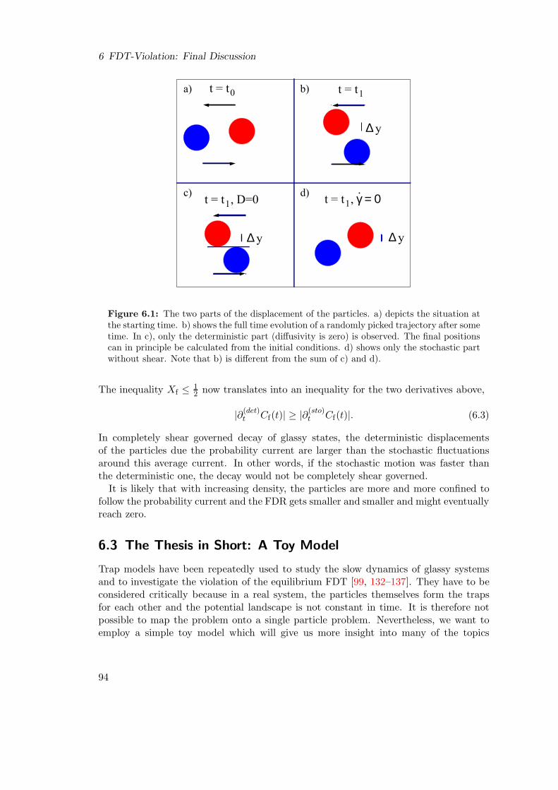
6 FDT-Violation: Final Discussion
0t = t
.1 1t = t , γ = 0
∆ y
t = t , D=0
∆ y
t = t1
∆ y
a) b)
c) d)
Figure 6.1: The two parts of the displacement of the particles. a) depicts the situation atthe starting time. b) shows the full time evolution of a randomly picked trajectory after sometime. In c), only the deterministic part (diffusivity is zero) is observed. The final positionscan in principle be calculated from the initial conditions. d) shows only the stochastic partwithout shear. Note that b) is different from the sum of c) and d).
The inequality Xf ≤ 12 now translates into an inequality for the two derivatives above,
|∂(det)t Cf(t)| ≥ |∂(sto)
t Cf(t)|. (6.3)
In completely shear governed decay of glassy states, the deterministic displacementsof the particles due the probability current are larger than the stochastic fluctuationsaround this average current. In other words, if the stochastic motion was faster thanthe deterministic one, the decay would not be completely shear governed.
It is likely that with increasing density, the particles are more and more confined tofollow the probability current and the FDR gets smaller and smaller and might eventuallyreach zero.
6.3 The Thesis in Short: A Toy Model
Trap models have been repeatedly used to study the slow dynamics of glassy systemsand to investigate the violation of the equilibrium FDT [99, 132–137]. They have to beconsidered critically because in a real system, the particles themselves form the trapsfor each other and the potential landscape is not constant in time. It is therefore notpossible to map the problem onto a single particle problem. Nevertheless, we want toemploy a simple toy model which will give us more insight into many of the topics
94

6.3 The Thesis in Short: A Toy Model
a
b
Figure 6.2: The toy model: The particle is trapped in wells of width a with infinitely highpotential barriers. The center-to-center distance of the wells is denoted b.
discussed in this thesis. As far as the author knows, this model has not been introducedbefore. The model for glassy states is depicted in Fig. 6.2: The particle, surroundedby solvent (diffusivity D0 = kBTµ0), is trapped in an infinite potential well of width a.This potential well is one in a row of infinitely many with center-to-center distances b.Since these potential wells look very much like water glasses, the particle is literally “inthe glass”. The particle performs a stochastic motion in this well, and a very long timeafter we measured its position, its probability distribution P (x) is constant within thewell and zero outside. We neglect the dimensions of the particle and restore physicalunits.
6.3.1 Shear Melts the Glass
Now we introduce the shear, i.e., a mechanism which lifts the particle over the potentialbarriers; At time t = τ, 2τ, 3τ, . . . , we introduce shear steps; The particle is put intoone of the neighboring wells according to its current position: If it is on the left side ofthe well, it gets to the well on the left hand side, if it is on the right hand side, it getsinto the well on the right hand side. We hence consider a direction perpendicular to theshear flow, where its influence is symmetric. The position at which the particle entersthe new well is not important, it shall be distributed randomly. The resulting dynamicshas some similarities to a Cauchy process [138].
6.3.2 Dynamics
The dynamics in our model shares many properties of colloidal suspensions. We regardthe limit of small shear rates, it corresponds to τ ≫ a2/D0, i.e., the time between twoshear steps is much longer than it takes the particle to relax in the well.
Short Times
At short times, the mean squared displacement of the particle is the one of a free particle,
limt→0
〈(x − x(0))2〉 = 2D0t. (6.4)
95

6 FDT-Violation: Final Discussion
Intermediate Times
For times τ > t ≫ a2/D0, the dynamics of the particle is glassy, i.e., the MSD isconstant on the plateau. This plateau value can be derived from the constant probabilitydistribution of the particle in the well, P (x) = 1/a,
〈(x − x(0))2〉 =1
a2
∫ a/2
−a/2dx(0)
∫ a/2
−a/2dx(x − x(0))2 =
a2
6, τ > t ≫ a2/D0. (6.5)
We notice that in accordance with the glassy dynamics of colloidal suspensions, theplateau value is independent of D0 and temperature. Note that the average over initialconditions is important in Eq. (6.5). The initial conditions are distributed with P (x) aswell.
Long Times
At every shear step the particle jumps to the left or right with equal probability, per-forming a random walk with step-length b and number of steps t/τ 1. After many steps,the contribution of the plateau value to the MSD becomes negligible,
〈(x − x(0))2〉 = b2 t
τ, t ≫ τ. (6.6)
The long time dynamics is independent of temperature and short time diffusivity D0,as is the long time decay of the density correlator for colloidal glasses, compare thediscussion in Sec. 1.6. The timescale is set by the period τ .
6.3.3 Mobility
To calculate the fluctuation dissipation ratio X, we have to find the mobility µ(t) ofthe particle in response to a small test force F acting on the particle. We assume thatthis test force does not influence the game rules defined above: At the shear step, theparticle gets to the left if it is on the left hand side of the well, and to the right, if it is onthe right hand side of the well. Recall the FDT (the Einstein relation) in equilibrium,
µ(t) =1
2kBT
∂
∂t〈(x − x(0))2〉. (6.7)
It is more convenient to study the integrated version,
1
F〈(x − x(0))〉(F ) =
1
2kBT〈(x − x(0))2〉. (6.8)
〈. . . 〉(F ) denotes an average under the influence of the external force.
1We ignore the fact that the movement is discontinuous.
96

6.3 The Thesis in Short: A Toy Model
F.
Figure 6.3: The long time probability distribution of the particle in the well without (red)and with external force (blue). This probability function for the real hard sphere system iscalculated as function of external force within mode coupling theory in Ref. [118].
Short Times
At short times the particle obeys the FDT (6.8) and the mean traveled distance is
limt→0
1
F〈(x − x(0))〉(F ) = µ0t =
1
kBTD0t. (6.9)
Intermediate Times
The external force influences the probability distribution of the particle in the well, seeFig. 6.3. It is more likely to find the particle in the right hand side of the well than onthe left hand side. The probability distribution PF (x) for τ > t ≫ a2/D0 follows theBoltzmann distribution [20], which, in linear order of the external force, reads,
PF (x) =
1a
(
1 + F xkBT
)
−a/2 < x < a/2,
0 else,τ > t ≫ a2/D0. (6.10)
The mean traveled distance is easily derived,
1
F〈(x − x(0))〉(F ) =
1
a
∫ a/2
−a/2dx(0)
∫ a/2
−a/2dxPF (x)(x − x(0)) =
a2
12kBT. (6.11)
Comparing with Eq. (6.5), the Einstein relation (6.8) holds for all times t < τ as ex-pected.
Long Times
Due to the distorted probability distribution PF (x) in Eq. (6.10), the particle will morelikely jump to the right at the shear step at t = τ . The rate R for jumps to the rightminus the rate for jumps to the left follows,
R =
∫ a/20 PF (x)dx −
∫ 0−a/2 PF (x)dx
∫ a0 PF (x)dx
=a
4
F
kBT+ O(F 2). (6.12)
97

6 FDT-Violation: Final Discussion
At every shear step, the particle travels on average the distance bR. For t ≫ τ , theinitially traveled distance in the well is negligible and we have
1
F〈(x − x(0))〉(F ) =
a b
4kBT
t
τ, t ≫ τ. (6.13)
The mobility of the particle is finite at long times and independent of the diffusivity D0.
6.3.4 Long Time FDR
Comparing Eqs. (6.13) and (6.6), we see that the Einstein relation does not hold for longtimes. The long time FDR X(t ≫ τ) is different from unity,
X(t) =
1 t < τ,12
ab t ≫ τ.
(6.14)
The FDT violation at long times comes from the fact that the shear steps are ‘unbend-able’, i.e., their step-length is not influenced by the external force. Once the position ofthe particle in the well has been identified at the shear step, the dynamics is determin-istically going to the appointed well. In some cases even to the left well, i.e., against theexternal force. The external force has no means to prevent this. We believe that thesame happens in the real system under shear.
We note that X(t ≫ τ) is independent of temperature because the potential bar-riers are infinitely high. We found the same for the hard sphere system in Chap. 4.In simulations of soft spheres, this is not true because the temperature also governsthe glass transition. We observe that the FDR in our model depends on the ratio of“stochastic diffusion length” a and “deterministic diffusion length” b. This illuminatesour interpretation in Sec. 6.1.
We note that X(t ≫ τ) reaches 12 if b goes to a. b < a (leading to 1 > X > 1
2) isphysically not reasonable, therefore there is an excluded region for the value of the FDRin the glass, as we found for the real system. This range coincides with the one we foundin Chap. 4.
The model allows to discuss two more effects: In the real system at increasing density,the cages become smaller and smaller, i.e., in our model we have a decreasing value ofab and X(t ≫ τ) decreases in accordance with the real system in Fig. 4.13. In the toymodel, it eventually reaches zero being always positive.
For increasing shear rates, i.e., decreasing τ , the particle has less time to relax in thewell and the effect of the external force decreases, this leads to a decreasing value ofX. This is also in agreement with our calculation in Chap. 4, see Fig. 4.13 and thesimulations in Ref. [1]. We believe that the decrease in the real colloidal system hasthe same origin, i.e., the particle has less time to adjust its distribution in the cage inresponse to the force.
6.3.5 The Comoving Frame
Our simple model also allows to illustrate the dynamics in the frame comoving with theprobability current because the latter is simply given by the shear steps between the
98

6.3 The Thesis in Short: A Toy Model
1 2 3 4 56 7 8
1 2 46 8
label 1 2 3 4 5 6 7 8
time 0 τ − δt τ + δt 2τ − δt 2τ + δt 3τ − δt 3τ + δt 4τ − δt
Figure 6.4: The real dynamics (top) and the dynamics in the comoving frame (bottom).The positions correspond to times given in the table. The particle diffuses in the well andis at position 2 when the shear step happens. This shear step takes the particle to position3 from where it diffuses to position 4 from where it is taken away by the next shear stepand so on. On the bottom, we show the movement in the comoving frame. Positions 2 and3, 4 and 5, and 6 and 7 coincide. The traveled distance is shorter, but the particle will getinfinitely far away in contrast to the case without shear steps.
potential wells. Fig. 6.4 illustrates the dynamics in the comoving frame. It is slowerthan in the rest-frame but still ergodic in contrast to the case without shear steps. Wesee that in the comoving frame, the position of the well is changed at every shear step.It is clear that the mobility of the particle obeys the FDT at all times in this system.
6.3.6 The Waiting Time Derivative
Our relation for the waiting time derivative in Eq. (2.18) is the central approximation ofthis thesis. The toy model can give further insight into this approximation although itdoes not contain the difference between stationary or transient dynamics. How can weintroduce a small waiting time tw in the toy model? For tw = δt, we simply have shearsteps at t = τ − δt, 2τ − δt, . . . , i.e., they are shifted by −δt. This is in agreement to thereal system, where for tw = δt the cages break at tbreak − δt if they break at tbreak fortw = 0. With this and Sec. 6.3.2 we find
limδt→0
⟨(x − x(0))2
⟩(t, tw = δt) =
⟨(x − x(0))2
⟩(t, tw = 0) t < τ − δt,
⟨(x − x(0))2
⟩(t + δt, tw = 0) t ≫ τ.
(6.15)
The derivative with respect to waiting time at tw = 0 is zero for t < τ and equal tothe time derivative for t ≫ τ , i.e., it is the long time derivative in accordance to ourapproximation in Chap. 2. Of course, the way we introduced the waiting time into themodel was chosen such that this result is achieved, but it still illustrates our intuitiveargument in Sec. 2.5.3.
99

7 Summary and Outlook
In this thesis, different properties of colloidal suspensions near the glass transition undershear are analyzed. We saw that the difference between the transient and the stationarycorrelator is largest at intermediate times. This effect is attributed to the fact that in thecase of the transient correlator, all particles are mobilized simultaneously at a certainstrain, whereas in the steady state, the particles escape their cages every now and then,uncorrelated to the correlation time t. Hence, the steady correlator decays earlier fromthe glassy plateau. We saw that the dependence on waiting time after switch-on can bevery accurately described for small waiting times. This prediction awaits experimentaltests. The same is true for our formula for long waiting times, which one might also beable to improve in the future.
A tagged particle shows anisotropic dynamics under shear. This anisotropy is verysimple near the critical plateau, it shows the expected “quadrupole”-behavior: Twoopposite poles on the unit sphere in wavevector space have slightly faster dynamics, theother two poles have slightly slower dynamics. This prediction also awaits experimentaltests. We saw that the mean squared displacement of the tagged particle is anisotropicas well. In the direction of the shear flow it shows a term that grows cubically in time.The amplitude of this term is connected to the diffusivity in the gradient direction asis the case for low densities where the phenomenon is known as Taylor dispersion. Thisholds even for glassy states where all terms show the characteristic yield scaling withshear rate. We found agreement to recent simulations.
Focus was put on the violation of the fluctuation dissipation theorem. We saw thatthe largest of the terms that violate the FDT can be related to the difference betweentransient and stationary correlators. This led us to a universal non-equilibrium ratiobetween response and fluctuations in the simplest approximation, namely an FDR ofX = 1
2 for glassy states at long times. This is in agreement with the notion of aneffective temperature proposed previously. Intriguingly, this value was also found indifferent spin models before. Looking more closely, we find corrections to this valuewhich depend on observable and which alter X to values smaller than 1
2 in glassy states.This dependence on observable contradicts the notion of an effective temperature. Weidentified all but one of the terms that violate the fluctuation dissipation theorem withwell defined measurable quantities. With this, all our approximations can in principle betested independently. It would be a great joy for the author if someone would identifythe last one of the violating terms with a measurable quantity in the future.
Studying the microscopic form of the susceptibility, we found that it contains not thefull Smoluchowski operator (SO) in front of the time evolution exponential, which wouldgive the time derivative, but only part of it. The SO is not Hermitian under shear andit is exactly its Hermitian part which enters the susceptibility. The Hermitian part can
100

be shown to represent the dynamics in the frame comoving with the 3N -dimensionalprobability current. We concluded that the equilibrium FDT holds in the comovingframe.
Finally we attributed the violation of the equilibrium FDT to the deterministic part ofthe dynamics to which the susceptibility is not sensitive. The deterministic part is givenby the dynamics following the average probability current. This led us to the conclusionthat the deterministic part is as large as the stochastic part at X = 1
2 , illuminating thespecialty of this value. We argued that the FDR must always be less than unity. Ina very simple toy model, which shares many properties of the real colloidal system, wewere able to study the FDT violation more closely. We saw that the violation appearsdue to the deterministic part of the dynamics and we were able to visualize the dynamicsin the comoving frame.
101

8 Zusammenfassung
In der vorliegenden Arbeit werden Eigenschaften von kolloidalen Glasern unter dem Ein-fluß von Scherung untersucht. Dieses System ist im Nichtgleichgewicht und erreicht einenstationaren Zustand, wenn man ausreichend lang eine konstante Scherung anlegt. Ins-besondere wird das Fluktuations-Dissipations-Theorem (FDT) studiert. Dieses gilt imGleichgewicht und verbindet die Antwort des Systems auf eine kleine externe Kraft mitden thermischen Fluktuationen des ungestorten Systems. Im Nichtgleichgewichtssystemunter Scherung ist das FDT verletzt. In Computersimulationen [1] wurde gefunden, dassdas FDT in gescherten Glasern auf sehr spezielle Weise verletzt ist. Das Gleichgewichts-FDT scheint zu gelten wenn man die Temperatur des Systems durch einen anderen Wertersetzt, die so genannte effektive Temperatur.
Die Arbeit beginnt mit der Analyse verschiedener Korrelationsfuntionen. Dies istnotig, da sich die Kenntnis der Unterschiede zwischen diesen als erforderlich fur dasStudium des FDT herausstellte. Der transiente Korrelator beschreibt thermische Fluk-tuationen, deren Messung beim Einschalten der externen Scherung beginnt. Beginnt dieMessung eine Zeitspanne nach dem Einschalten der Scherung, d.h. nach der sogenanntenWartezeit, so wird der Zwei-Zeiten-Korrelator gemessen. Im Limes großer Wartezeitenerreicht dieser den stationaren Korrelator, der die Fluktuationen im stationaren Zus-tand beschreibt. Der Unterschied zwischen diesen Korrelatoren wird untersucht, wobeiinsbesondere eine sehr genaue Beschreibung der Abhangigkeit des Korrelators von derWartezeit fur kurze Wartezeiten erreicht wird. Diese Beschreibung fur kurze Wartezeitenkann in Computersimulationen getestet werden.
Im dritten Kapitel wird die Dynamik eines einzelnen markierten Teilchens studiert,eine Erwartungsgroße, die im Bezug auf die Verletzung des FDTs im vierten Kapitelvon Bedeutung sein wird: In den Computersimulationen wird besonders die Verletzungdes FDT fur einzelne markierte Teilchen untersucht. Unsere Untersuchungen ergeben,dass das mittlere Verschiebungsquadrat des Teilchens in Richtung des Scherflusses furlange Zeiten nicht wie in Diffusionsprozessen linear in der Zeit wachst, sondern kubisch.Dies ist fur kolloidale Losungen niedriger Dichte bekannt als Taylor Dispersion. Wirfinden, dass der kubische Term mit der Diffusion des Teilchens in Gradientenrichtungverknupft ist. Diese Verknupfung ist identisch zu derjenigen, die bei niedrigen Dichtenauftaucht. Dies gilt sogar fur Glaser, wo alle Diffusionskonstanten die charakteristischelineare Skalierung mit der Scherrate zeigen.
Das Studium der Verletzung des FDTs unter Scherung ergibt, dass der Term, der dengroßten Beitrag zur Verletzung liefert, mit der Abhangigkeit des Zwei-Zeiten-Korrelatorsvon der Wartezeit verknupft ist. Wir verbinden somit zwei vollig verschiedene experi-mentelle Meßgroßen. Das fuhrt uns auf ein universelles Nichtgleichgewichts-Verhaltnisvon Antwortfunktion und Fluktuationen in der einfachsten Naherung, das Fluktuations-
102

Dissipations-Verhaltnis (FDR) X nimmt den Wert X = 12 an. Dies ist in Ubereinstimmung
mit der vorgeschlagenen Beschreibung mithilfe einer effektiven Temperatur. Der WertX = 1
2 wurde interessanterweise vorher auch in kritischen Spin-Modellen gefunden.Wenn man genauer hinschaut, gibt es Korrekturen zu diesem Wert, die von der studiertenObservablen abhangen. Diese Abhangigkeit widerspricht der Interpretation einer effek-tiven Temperatur. Es ergibt sich, dass das FDR in Glasern kleiner als 1
2 ist.Anschließend untersuchen wir die mikrospkopische Form der Suszeptibilitat genauer.
Wir finden, dass die Antwortfunktion nicht durch die volle Zeitableitung der Korre-lationsfunktion gegeben ist, wie das im Gleichgewicht der Fall ist, sondern nur durcheinen Teil der Ableitung. Dieser Teil kann interpretiert werden als Ableitung im System,das sich mit dem stationaren Wahrscheinlichkeitsstrom mitbewegt. Dieser Wahrschein-lichkeitsstrom hat 3N Komponenten, wobei N die Teilchenzahl ist. Wir folgern, dassman die Dynamik des Systems in einen stochastischen und einen deterministischen Teil(gegeben durch den Wahrscheinlichkeitsstrom) aufteilen kann, wobei die Antwortfunk-tion nur den stochastischen Teil misst. Sie ist damit kleiner, als man vom Gleichgewichts-FDT erwarten wurde. Der spezielle Wert von X = 1
2 kann damit so interpretiert werden,dass stochastischer und deterministischer Teil genau gleich groß sind. Zuletzt betrachtenwir ein einfaches Spielzeug-Modell, das viele Eigenschaften glasartiger kolloidaler Sus-pensionen teilt. Es erlaubt uns, die Verletzung des FDTs zu studieren. Wir sehen, dassdiese Verletzung vom deterministischen Anteil der Dynamik verursacht wird.
103

A β-Analysis
For 0 ≤ ε ≪ 1 and γt ≪ 1, the correlators are expanded near the critical plateau
Φq(t) = f cq + (1 − f c
q )2Gq(t), (A.1a)
Φsq(t) = f sc
q + (1 − f scq )2Gs
q(t), (A.1b)
where the isotropic Gq(t) for the coherent correlator is known, Gq = Geq, with eq theeigenvector with eigenvalue unity of the stability matrix of the coherent memory function[10, 27]. Eq. (3.42) is recovered by (1−f c
q )2 eq = hq. We rename the incoherent memoryfunction in traditional MCT notation1,
msq(t, t′) = Fq(t, t′,Φk,Φs
p). (A.2)
It is for γ = 0 given by Feq (Φ
(e)k ,Φ
s(e)p ). Expanding it around the critical value, where
superscripts c and e denote critical parameters and equilibrium respectively, one has
Fq(t, t′,Φk,Φsp) = Fc,e
q (f c, f sc) +∑
k
Cc,eq,kGk(t − t′) +
∑
k
Cc,e,sq,k Gs
k(t − t′)
+∆F (γ)q (t, t′, f c
q , f scp ) + . . . . (A.3)
The last term, ∆F (γ)q , is the contribution in lowest order in γt and γt′ of the advection
in the vertices. The Taylor coefficients read
Cc,eq,k =
∂Fc,eq (f, f s)
∂f
∣∣∣∣fc,fsc
(1 − f ck)2, (A.4a)
Cc,e,sq,k =
∂Fc,eq (f, f s)
∂f s
∣∣∣∣fc,fsc
(1 − f sck )2. (A.4b)
Only the critical Taylor coefficients appear in Eq. (A.3), because higher order terms areof order ε [10] and hence of order G2. With Eq. (A.3), the equation of motion, Eq. (3.38)becomes for long times (divided by (1 − f sc
q )),
f scq
1 − f scq
−Fc,eq (f c, f sc) + Gs
q(t) =∑
k
Cc,eq,kGk(t) +
∑
k
Cc,e,sq,k Gs
k(t)
+∆F (γ)q (t, 0, f c
q , f scp ) + . . . . (A.5)
1Fq is different from the function introduced in Eq. (1.25). We do not want to use the superscript s
here because of the many superscripts it will carry below.
104

The first two terms cancel each other since they fulfill the equation for the plateau valuef s
q [77],f s
q
1 − f sq
= Feq (f, f s). (A.6)
Eq. (A.5) is not singular at the critical density [10] and we can solve the linear equationfor Gs
q,∑
k
(δq,k − Cc,e,sq,k )Gs
k(t) =∑
k
Cc,eq,kGk(t) + ∆F (γ)
q (t, 0, f cq , f sc
p ). (A.7)
We notice that the anisotropic part of Gsk(t) is eigenfunction of the eigenvalue zero of
the matrix Cc,e,sq,k , because it is antisymmetric in qx and qy as we will see below. The
isotropic and the anisotropic part of the equation separate. We find that the solution ofthe isotropic part is given by the coherent β-correlator with a q-dependent pre-factor,
G(s,iso)q (t) = es
qG(t). The equation for this pre-factor is given by
∑
k
(δq,k − Cc,e,sq,k )es
k =∑
k
Cc,eq,kek. (A.8)
Eq. (A.8) is identical to the corresponding equation for the equilibrium case in Ref. [77].The critical amplitude for the incoherent correlator is thus given by its equilibrium value,
hsq = (1 − f sc
q )2esq. (A.9)
Eq. (3.47) for the anisotropic term follows with (we insert the pre-factor of (1−f scq )2/hs
q
to be able to compare the anisotropic part directly to G(t)),
(1 − f scq )2
hsq
∆F (γ)q (t, 0, f c
q , f scp ) ≡ G(s,aniso)
q (t) = G(q) γt + O(γt)2. (A.10)
105

B Approximations for nq(t)
We show the derivation of the expressions for the memory functions used in Sec. 4.5 indetail. The time dependent pair density projector is given by [60],
P2(t) =∑
k>p,k′>p′
k(t)p(t)〉〈∗k′(t)∗p′(t)
〈∗k(t)
∗p(t)k′(t)p′(t)〉
≈∑
k>p
k(t)p(t)〉〈∗k(t)∗p(t)
N2Sk(t)Sp(t). (B.1)
The triple density projector is used less often in the literature [139–141]. It followsdirectly from the pair projector,
P3(t) =∑
k>p>n,k′>p′>n′
k(t)p(t)n(t)〉〈∗k′(t)∗p′(t)
∗n′(t)
〈∗k(t)
∗p(t)
∗n(t)k′(t)p′(t)n′(t)〉
≈∑
k>p>n
k(t)p(t)n(t)〉〈∗k(t)∗p(t)
∗n(t)
N3Sk(t)Sp(t)Sn(t). (B.2)
The memory function n(1)q has only one time evolution operator and can hence be ap-
proximated via “standard” routes with the projector P2(t) [60],
n(1)q (t) ≈ γ
2NS(γ)q Γq
⟨
σxy∗qQP2(−t)U(t)P2Ω
†q
⟩
. (B.3)
For the appearing time dependent four point correlation function, the MCT factorizationapproximation is used
〈∗k′(−t)∗k′(−t)−qU(t)kk−q〉 ≈ N2Sk(−t)Sk(−t)−qΦk(−t)(t)Φk(−t)−q(t)δk,k′ . (B.4)
At the left hand side appears the expression
V(1)qk =
⟨σxy
∗qQkq−k
⟩
NSq≈ kx(ky − qy)
S′q−k
q − kSk + kxky
S′k
kSq−k. (B.5)
On the right hand side, we have the standard vertex
V(2)qk
=
⟨kq−kQΩ†q
⟩
NSk−qSk= q · ((k − q)nck−q + knck). (B.6)
In the derivation of Eqs. (B.5) and (B.6), the convolution approximation for the staticthree point correlation function was used [10],
〈qk−qk〉 ≈ NSq Sk−q Sk. (B.7)
106

Improvements for this formula have been discussed in Refs. [61, 142, 143]. The approx-imation for the function mq(t) is achieved in a similar way, the vertex (B.6) appearingon both sides of the time evolution operator [60]. The term of order γ, which appearsin the left vertex when approximating Eq. (4.37), is neglected.
The treatment of n(2,3)q is more involved. We first separate the time evolution operator
in t with pair projectors to get,
n(2)q (t) ≈ γ
2NS(γ)q Γq
∫ ∞
0ds⟨
σxyeΩ†s∗qΩ† QP2U(t)P2(t)QΩ†q
⟩
, (B.8)
n(3)q (t) ≈ −γ
2NS(γ)q Γq
∫ ∞
0ds⟨
σxyeΩ†s(Ω†∗q)QP2U(t)P2(t)QΩ†q
⟩
. (B.9)
After doing this, we are on the left hand side of the projectors left with the two respectiveexpressions, ⟨
σxyeΩ†s∗qΩ† Qq−kk
⟩
, (B.10)
and ⟨
σxyeΩ†s(Ω†∗q)Qq−kk
⟩
. (B.11)
Writing Q as 1 − P , we realize that the term containing P is identical for both terms(they are real),
⟨
σxyeΩ†s(Ω†∗q) q
⟩ 1
NSq
⟨∗qq−kk
⟩, (B.12)
with opposite sign. These terms cancel each other. We are left with the two expressions,
⟨
σxyeΩ†s∗qΩ†q−kk
⟩
, (B.13)
and ⟨
σxyeΩ†s(Ω†∗q)q−kk
⟩
. (B.14)
Now there is in principal more than one option to treat these terms, but we will arguethat only one option is applicable. The standard way, i.e., the usage of P2 right and leftof the time evolution operator is not preferable since it would not preserve the derivativewith respect to s. As already mentioned, this derivative is necessary for the correctγ-dependence. Also, this treatment would lead to a static five point correlation, whosefurther treatment would be delicate. Another option would be to use only one pairprojector on the left hand side of the evolution operator. This would lead us to a timedependent five point correlation which is even more delicate. That is why we chose touse the triple densities projector P3. The first of the expressions, Eq. (B.13) is writtenas
⟨
σxyeΩ†s∗qΩ†q−kk
⟩
≈⟨
σxyP3(−s)eΩ†s∗qΩ†q−kk
⟩
. (B.15)
It is now clear that we have to demand that the wavevectors in the triple projectortake the values of the wavevectors on the right hand side. Due to this constraint,
107

B
the summation over wavevectors in Eq. (B.2) contains only one term and no counting
factor appears. The left hand side is just the Vertex V(1)qk in Eq. (B.5) for s–dependent
wavevectors. Note that in (B.5), the projector Q does not make any difference. Theappearing six point s-dependent correlation function is approximated as,
〈∗q∗k(−s)
∗k(−s)−q
eΩ†sqΩ†kk−q〉N3SqSk(−s)−qSk(−s)
≈ Φq(s)
([∂
∂s− k(−s) · ∂
∂k
]
Φk(−s)(s)Φk(−s)−q(s)
)
.
(B.16)This approximation rests on the observation that the operator Ω† acts as an s derivative.Φk(−s)(s) and Φk(−s)−q(s) depend on s via the decay of the correlator and via the s–
dependent wavevectors. Since Ω† in (B.16) represents the s–derivative with respectto correlator dynamics, we have to subtract the change in s due to the change of thewavevectors. The term in Eq. (B.14) is treated analogously with the triple densityprojector. Here, the approximation for the appearing six point correlation function ismore straight forward, since Φq(s) has no wavevector advection,
〈∗q∗k(−s)
∗k(−s)−q
eΩ†s(Ω†q)kk−q〉N3 Sq Sk(−s)−q Sk(−s)
≈(
∂
∂sΦq(s)
)
Φk(−s)(s)Φk(−s)−q(s). (B.17)
The expressions in Eqs. (4.51a – 4.51c) follow.
108

C Approximations for nsq(t)
The terms in Eq. (4.60) are approximated similarly to the coherent analogues, using
the pair density projector in Eq. (3.34). The approximation for n(s,1)q (t) is then straight
forward following Eqs. (B.3-B.5). Regarding the vertex, there occur simplifications,
V(s,1)qk =
⟨σxy
s∗q Qsks
q−k
⟩= kxky
S′k
k. (C.1)
The right hand side of the vertex is identical to Eq. (3.37),
V(s,2)qk
=
⟨
sk−q−k Qs Ω†
esq
⟩
Sk= k · qn cs
k. (C.2)
For the memory functions n(s,2)q (t) and n
(s,3)q (t) we first use the projector P s
2 accordingto Eqs. (B.8) and (B.9). We note that the term corresponding to Eq. (B.12), whichcancels, vanishes here in both terms independently, see the discussion around Eq. (3.55).We arrive at the expressions equivalent to Eqs. (B.13) and (B.14), reading
⟨
σxyeΩ†ss∗
q Ω†sq−kk
⟩
, (C.3)
and⟨
σxyeΩ†s(Ω†s∗
q )sq−kk
⟩
. (C.4)
On first sight, it seems not necessary to use the triple density projector here, since thedensities on the right hand side might reduce to a pair density and the dependence onsq might drop out. The author did not find a way to perform this simplification while
conserving the interpretation of the derivative with respect to s, which is necessary toachieve the correct γ-dependence. We hence use the triple density projector
P s3 (t) ≈
∑
k>p>n
sk(t)
sp(t)n(t)〉〈s
k(t)sp(t)n(t)
NSn(t), (C.5)
109
C
according to Eq. (B.15). The discussions around Eqs. (B.16) and (B.17) hold. We finallyarrive at
n(s,1)q (t) =
γ
2nq2
∫d3k
(2π)3V
(s,1)qk(−t)V
(s,2)qk Φk(−t)(t)Φ
sk(−t)−q(t), (C.6a)
n(s,2)q (t) =
γ
2nq2
∫ ∞
0ds
∫d3k
(2π)3V
(s,1)qk(−s)V
(s,2)qk(t)Φ
sq(s)
([∂
∂s− k′(−s) · ∂
∂k
]
Φk(−s)(s)Φsk(−s)−q(s)
)
Φk(t)Φsk−q(t), (C.6b)
n(s,3)q (t) =
−γ
2nq2
∫ ∞
0ds
∫d3k
(2π)3V
(s,1)qk(−s)V
(s,2)qk(t)
(∂
∂sΦs
q(s)
)
Φk(−s)(s)Φsk(−s)−q(s)Φk(t)Φs
k−q(t). (C.6c)
We evaluate these expressions numerically, using the approximation (4.54) for the co-herent correlator and a similar approximation for the incoherent one, motivated bythe solution for the correlator near the critical plateau in Eq. (3.53). We neglect theanisotropic part and write for long times in glassy states
Φsq(t) ≈ Φs
q(t) = f sq exp
(
−hs
q
f sq
c |γ|t)
. (C.7)
We use again c = 3. We consider the case where the tagged particle has the same sizeas the bath particles, for which cs
q = (Sq − 1)/(nSq) holds. For the numerical evaluationof (C.6), we use the grid kmax = 25, ∆k = 0.2, ∆θ = π/40 and ∆φ = π/20 (z-direction)and ∆θ = π/20 and ∆φ = π/64 (y-direction) or smaller to account for the differentsymmetries in the different directions. The time was discretized as in the coherentcase.
110

Bibliography
[1] L. Berthier and J.-L. Barrat. J. Chem. Phys. 116, 6228 (2002).
[2] R. G. Larson. The Structure and Rheology of Complex Fluids (Oxford UniversityPress, New York, 1999).
[3] P. N. Pusey and W. Van Megen. Nature 320, 340 (1986).
[4] P. N. Pusey and W. van Megen. Phys. Rev. Lett. 59, 2083 (1987).
[5] W. van Megen and P. N. Pusey. Phys. Rev. A 43, 5429 (1991).
[6] W. van Megen and S. Underwood. Phys. Rev. Lett. 70, 2766 (1993).
[7] W. van Megen and S. Underwood. Phys. Rev. E 49, 4206 (1994).
[8] W. van Megen, T. C. Mortensen, J. Muller, and S. R. Williams. Phys. Rev. E 58,6073 (1998).
[9] P. Hebraud, F. Lequeux, J. Munch, and D. J. Pine. Phys. Rev. Lett. 78, 4657(1997).
[10] W. Gotze. Liquids, freezing and glass transition ed J.-P. Hansen, D. Levesque andJ. Zinn-Justin (Amsterdam, 1991) p 287.
[11] Soft and fragile Matter ed M. E. Cates and M. R. Evans (Scottish UniversitiesSummer School in Physics & Institute of Physics Publishing, Bristol & Philadel-phia).
[12] R. Besseling, E. R. Weeks, A. B. Schofield, and W. C. K. Poon. Phys. Rev. Lett.
99, 028301 (2007).
[13] J. J. Crassous, M. Siebenburger, M. Ballauff, M. Drechsler, D. Hajnal, O. Henrich,and M. Fuchs. J. Chem. Phys. 128, 204902 (2008).
[14] J. Zausch, J. Horbach, M. Laurati, S. Egelhaaf, J. M. Brader, Th. Voigtmann, andM. Fuchs. J. Phys.: Condens. Matter 20, 404210 (2008).
[15] J. K. G. Dhont. Phys. Rev. E 60, 4534 (1999).
[16] J. Bender and N. J. Wagner. J. Rheol. 40, 899 (1996).
[17] C. B. Holmes, M. E. Cates, M. Fuchs, and P. Sollich. J. Rheol. 49, 237 (2005).
111
Bibliography
[18] M. Fuchs. Advances in Polymer Science Submitted, ArXiv:0810.2505 (2008).
[19] J. Bergenholtz. Current Opinion in Colloid & Interface Science 6, 484 (2001).
[20] J. K. G. Dhont. An Introduction to Dynamics of Colloids (Elsevier science, Ams-terdam, 1996).
[21] M. Fuchs and M. E. Cates. J. Phys.: Cond. Mat. 17, 1681 (2005).
[22] H. Risken. The Fokker-Planck Equation (Springer, Berlin, 1984).
[23] E. D. Elrick. Austral. J. Phys. 15, 283 (1962).
[24] G. I. Taylor. Proc. Roy. Soc. A 219, 186 (1953).
[25] G. I. Taylor. Proc. Roy. Soc. A 223, 446 (1954).
[26] G. I. Taylor. Proc. Roy. Soc. A 225, 473 (1954).
[27] M. Fuchs and M. E. Cates. Faraday Discuss. 123, 267 (2003).
[28] M. Fuchs and M. E. Cates. Phys. Rev. Lett. 89 (2002).
[29] J.-P. Hansen and I. R. McDonald. Theory of Simple Liquids – 2nd ed. (Academicpress limited, London, 1986).
[30] R. Zwanzig. J. Chem. Phys. 33, 1338 (1960).
[31] R. Zwanzig. Phys. Rev. 124, 983 (1961).
[32] H. Mori. Phys. Rev. 112, 1829 (1958).
[33] H. Mori. Prog. Theor. Phys. 33, 423 (1965).
[34] R. Zwanzig. Nonequilibrium Statistical Mechanics (Oxford University Press, 2001).
[35] U. Bengtzelius, W. Gotze, and A. Sjolander. J. Phys. C.: Solid State Phys. 17,5915 (1984).
[36] E. Leutheusser. Phys. Rev. A 29, 2765 (1984).
[37] W. Gotze and L. Sjogren. Rep. Prog. Phys. 55, 241 (1992).
[38] M. Fuchs. Transp. Theory Stat. Phys. 24, 855 (1995).
[39] H. Z. Cummins. J. Phys.: Condens. Matter 11, A95 (1999).
[40] M. E. Cates. Annales Henri Poincare 4, 647 (2003).
[41] S. P. Das. Rev. Mod. Phys. 76, 785 (2004).
[42] D. R. Reichman and P. Charbonneau. J. Stat. Mech. page P05013 (2005).
112

Bibliography
[43] K. Miyazaki and D. R. Reichman. Phys. Rev. E 66, 050501 (2002).
[44] K. Miyazaki, D. R. Reichman, and R. Yamamoto. Phys. Rev. E 70, 011501 (2004).
[45] T. Franosch, M. Fuchs, W. Gotze, M. R. Mayr, and A. P. Singh. Phys. Rev. E 55,7153 (1997).
[46] W. Gotze. Z. Phys. B 60, 195 (1985).
[47] M. Fuchs and M. Ballauff. J. Chem. Phys. 122, 094707 (2005).
[48] M. Fuchs and M. Ballauff. J. Chem. Phys. 125, 204906 (2006).
[49] R. Kubo, M. Toda, and N. Hashitsume. Statistitical Physics 2 (Springer, Berlin,1985).
[50] J. M. Brader, Th. Voigtmann, M. E. Cates, and M. Fuchs. Phys. Rev. Lett. 98,058301 (2007).
[51] J. M. Brader, M. E. Cates, and M. Fuchs. Phys. Rev. Lett. 101, 138301 (2008).
[52] W. Gotze. Z. Phys. B 56, 139 (1984).
[53] Th. Voigtmann. Schematische Modelle der Modenkopplungstheorie mit Hop-
pingterm (Diploma Thesis, Technische Universitat Munchen, 1998).
[54] M. Fuchs, W. Gotze, I. Hofacker, and A. Latz. J. Phys.: Condens. Matter 3, 5047(1991).
[55] Th. Voigtmann and M. Fuchs, unpublished.
[56] D. Hajnal. Scaling laws in the Rheology of Colloidal Dispersions (Diploma Thesis,Universitat Konstanz, 2007).
[57] A. W. Lees and S. F. Edwards. J. Phys. C.: Solid State Phys. 5, 1921 (1972).
[58] M. Fuchs and K. Kroy. J. Phys.:Condens. Matter 14, 9223 (2002).
[59] W. Gotze and A. Latz. J. Phys.:Condens. Matter 1, 4169 (1989).
[60] M. Fuchs and M. E. Cates. J. Rheol. Submitted (2008).
[61] O. Henrich, O. Pfeifroth, and M. Fuchs. J. Phys: Condens. Matter 19, 205132(2007).
[62] D. Hajnal, O. Henrich, J. J. Crassous, M. Siebenburger, M. Drechsler, M. Ballauffand M. Fuchs. AIP Conference Proceedings 1027, 674 (2008).
[63] Th. Voigtmann, private communication.
[64] M. Kruger and M. Fuchs. Phys. Rev. Lett. 102, 135701 (2009).
113

Bibliography
[65] F. Varnik. Complex Systems ed M. Tokuyama and I. Oppenheim (Amer. Inst. ofPhysics, 2008) p 160.
[66] F. Weysser, private communication.
[67] D. R. Foss and J. F. Brady. J. Fluid. Mech. 410, 243 (1999).
[68] A. Sierou and J. F. Brady. J. Fluid. Mech. 506, 285 (2004).
[69] A. M. Leshansky and J. F. Brady. J. Fluid. Mech. 527, 141 (2005).
[70] J. F. Morris and J. F. Brady. J. Fluid. Mech. 312, 223 (1996).
[71] K. Kawasaki and J. D. Gunton. Phys. Rev. A 8, 2048 (1973).
[72] M. Fuchs. Die α-Relaxation einfacher Flussigkeiten (PhD Thesis, Technische Uni-versitat Munchen, 1993).
[73] K. Kawasaki. Physica A 215, 61 (1995).
[74] B. Cichocki and W. Hess. Physica A 141, 475 (1987).
[75] F. G. Tricomi. Integral Equations (Interscience Publishers, New York, 1957).
[76] T. Franosch and W. Gotze. J. Phys.: Condens. Matter 6, 4807 (1994).
[77] M. Fuchs, W. Gotze, and M. R. Mayr. Phys. Rev. E 58, 3384 (1998).
[78] W. Gotze and L. Sjogren. J. Math. Anal. Appl. 195, 230 (1995).
[79] M. Fuchs, private communication.
[80] J. Bergenholtz, J. F. Brady, and M. Vivic. J. Fluid Mech. 456, 239 (2002).
[81] Th. Voigtmann, A. M. Puertas, and M. Fuchs. Phys. Rev. E 70, 061506 (2004).
[82] J. Zausch, private communication.
[83] G. Doetsch. Einfuhrung in Theorie und Anwendung der Laplace-Transformation
(Birkhauser, Stuttgart, 1970).
[84] L. Sjogren. Phys. Rev. A. 33, 1254 (1986).
[85] D. Forster. Hydrodynamic Fluctuations, Broken Symmetry, and Correlation Func-
tions (Benjamin, Reading, MA, 1975).
[86] A. Einstein. Annalen der Physik 17, 459 (1905).
[87] F. Schwabl. Statistische Mechanik (Springer, Berlin, 2000).
[88] F. Schwabl. Quantenmechanik fur Fortgeschrittene (Springer, Berlin, 2000).
114

Bibliography
[89] H. Nyquist. Phys. Rev. 32, 110 (1928).
[90] A. Crisanti and F. Ritort. J. Phys. A 36, R181 (2003).
[91] G. S. Agarwal. Z. Physik 252, 25 (1972).
[92] T. Speck and U. Seifert. Europhys. Lett. 74, 391 (2006).
[93] V. Blickle, T. Speck, C. Lutz, U. Seifert, and C. Bechinger. Phys. Rev. Lett. 98,210601 (2007).
[94] L. Berthier, J.-L. Barrat, and J. Kurchan. Phys. Rev. E 61, 5464 (2000).
[95] C. Godreche and J. M. Luck. J. Phys. A: Math. Gen. 33, 1151 (2000).
[96] C. Godreche and J. M. Luck. J. Phys. A: Math. Gen. 33, 9141 (2000).
[97] P. Calabrese and A. Gambassi. Phys. Rev. E 65, 066120 (2002).
[98] P. Mayer, L. Berthier, J. P. Garrahan, and P. Sollich. Phys. Rev. E 68, 016116(2003).
[99] P. Sollich, S. Fielding, and P. Mayer. J. Phys.: Condens. Matter 14, 1683 (2002).
[100] F. Corberi et al. J. Phys A: Math. Gen. 36, 4729 (2003).
[101] P. Calabrese and A. Gambassi. J. Stat. Mech.: Theo. Exp. page P07013 (2004).
[102] R. J. Glauber. J. Math. Phys. 4, 294 (1963).
[103] L. Berthier and J.-L. Barrat. Phys. Rev. Lett. 89, 095702 (2002).
[104] J.-L. Barrat and L. Berthier. Phys. Rev. E 63, 012503 (2000).
[105] C. S. O’Hern, A. J. Liu, and S. R. Nagel. Phys. Rev. Lett. 93, 165702 (2004).
[106] T. K. Haxton and A. J. Liu. Phys. Rev. Lett. 99, 195701 (2007).
[107] F. Zamponi, G. Ruocco, and L. Angelani. Phys. Rev. E 71, 020101 (2005).
[108] I. K. Ono, C. S. O’Hern, D. J. Durian, S. A. Langer, A. J. Liu, and S. R. Nagel.Phys. Rev. Lett. 89, 095703 (2002).
[109] J.-L. Barrat. J. Phys.: Condens. Matter 15, S1 (2003).
[110] J.-L. Barrat and W. Kob. Europhys. Lett. 46, 637 (1999).
[111] W. Kob and J.-L. Barrat. Eur. Phys. J. B 13, 319 (1999).
[112] A. Latz. J. Phys.: Condens. Matter 12, 6353 (2000).
[113] P. Ilg and J.-L. Barrat. Europhys. Lett. 79, 26001 (2007).
115

Bibliography
[114] J. S. Langer and M. L. Manning. Phys. Rev. E 76, 056107 (2007).
[115] N. Greinert, T. Wood, and P. Bartlett. Phys. Rev. Lett. 97, 265702 (2006).
[116] B. Abou and F. Gallet. Phys. Rev. Lett. 93, 160603 (2004).
[117] C. Maggi, R. d. Leonardo, J. C. Dyre, and G. Ruocco ArXiv:0812.0740 (2009).
[118] I. Gazuz, A. M. Puertas, Th. Voigtmann, and M. Fuchs. Phys. Rev. Lett. Submit-ted, ArXiv 0810.2627 (2008).
[119] P. Habdas, D. Schaar, A. C. Levitt, and E. R. Weeks. Europhys. Lett. 67, 477(2004).
[120] T. Harada and S. i. Sasa. Phys. Rev. Lett. 95, 130602 (2005).
[121] G. Szamel. Phys. Rev. Lett. 93, 178301 (2004).
[122] F. Varnik. J. Chem. Phys. 125, 164514 (2006).
[123] H. Zhang and G. Nagele. J. Chem. Phys. 117, 5908 (2002).
[124] J. A. McLennan. Introduction to Non-equilibrium Statistical Mechanics (PrenticeHall, New York, 1988).
[125] B. J. Berne and R. Pecora. Dynamic Light Scattering: With Applications to Chem-
istry, Biology and Physics (Dover Publications, Mineola, NY, 2000).
[126] M. Morse and H. Feshbach. Methods of Theoretical Physics, part 1 (McGraw-Hill,New York, 1953).
[127] R. Graham. Z. Physik B - Cond. Mat. 40, 149 (1980).
[128] L. D. Landau and E. M. Lifshitz. Course of Theoretical Physics, Volume 6: Fluid
Mechanics (Pergamon Press, Oxford, 1959).
[129] Monty Python, Monty Python and the Holy Grail, Scotland 1975.
[130] D. J. Pine, J. P. Gollub, J. F. Brady, and A. M. Leshansky. Nature 438, 997(2005).
[131] J. P. Gollub and D. J. Pine. Physics Today 59, 8 (2006).
[132] J. P. Bouchaud. J. Phys. I 2, 1705 (1992).
[133] A. Barrat and M. Mezard. J. Phys. I 5, 941 (1995).
[134] C. Monthus and J. P. Bouchaud. J. Phys. A 29, 3847 (1996).
[135] B. Rinn, P. Maass, and J. P. Bouchaud. Phys. Rev. Lett. 84, 5403 (2000).
[136] S. Fielding and P. Sollich. Phys. Rev. Lett. 88, 050603 (2002).
116

Bibliography
[137] S. M. Fielding, P. Sollich, and M. E. Cates. J. Rheol. 44, 323 (2000).
[138] C. W. Gardiner. Handbook of Stochastic Methods (Springer, Berlin, 1985).
[139] J. Schofield and I. Oppenheim. Physica A 181, 89 (1992).
[140] J. Schofield and I. Oppenheim. Physica A 187, 210 (1992).
[141] W. Gotze and L. Sjogren. J. Phys. C: Solid State Phys. 17, 5759 (1984).
[142] R. J. Baxter. J. Chem. Phys. 41, 553 (1964).
[143] J.-L. Barrat, J.-P. Hansen, and G. Pastore. Phys. Rev. Lett. 58, 2077 (1987).
117