protection for sale di er in crisis vs. economic stability ... · does \protection for sale"...

$: Protection for Sale di er in crisis vs. economic stability ... · Does \Protection for Sale" di er in crisis vs. economic stability times? (Evidence from ... import demand elasticity$
Does “Protection for Sale” differ in crisis vs. economic

stability times? (Evidence from Putin’s Russia)

Darya Gerasimenko∗

August 8, 2014

Preliminary draft - please do not quote without author’s permission.

Abstract

This paper assesses government trade policy making in crisis versus economic sta-

bility times using the Russian import tariff data (2001, 2005, 2009 and 2010) at the

industry level in Grossman and Helpman (1994) “Protection for sale” analytical

framework. I analyse the “Putin-Medvedev tandem” period starting in 2000 using

both tariff and non-tariff measures. The welfare mindedness of the government in

crisis (2009 and 2010) appears to be smaller relatively to the preceding economic

stability period in 2005. In other words, in crisis the government puts relatively

more weight on contributions from lobbyists. This result is driven by industry (or

firms) lobbying to obtain state support in hard times of financial difficulty and

by the government return to industrial policy. The residual regression analysis

supports this argument.

Keywords: Trade Policy, Tariff, Crisis, Protectionism, Protection for Sale, Wel-

fare, Russia

JEL Classification: D60, F13, F14, O24

Many thanks are due to Simon Evenett, Patrick Emmenegger, Marco Helm,

Patrick Low, Marcelo Ollareaga, Conny Wunsch as well as seminar participants

at the University of St. Gallen for their useful comments and suggestions; any

remaining errors are the author’s responsibility.

∗University of St.Gallen. E-mail: [email protected].

1 Introduction

In the last thirty years economists have paid increasing attention to determinants of trade

policy. Well known in the political economy literature Grossman and Helpman (1994)

“Protection for Sale” (PFS) model aims to explain the structure of trade policy. This

model emphasizes the influence of special interest groups (SIG) on government policy

by means of “political contributions” in a representative democracy. Organized interest

groups represent industries and are offering contributions, which politicians value for

their potential use in elections. The government chooses trade policy which maximizes

a weighted sum of aggregate welfare and total contributions from SIGs. The relative

preference of a government for aggregate welfare over contributions from a lobbyist is

known in the literature as the parameter “a” or “welfare mindedness” of the government.

Despite the parameter “a” is simplified in the government objective function, it contains

an interesting information when it is observed in dynamics (for various years) or across

different countries.

The empirical verification of the PFS model was conducted in several papers. Gold-

berg and Maggi (1999) and Gawande and Bandyopadhyaya (2000) present the first two

empirical studies using the United States non-tariff industry-level data. Both papers find

as predicted by Grossman-Helpman model that protection to organized sectors is nega-

tively related to import penetration and import demand elasticity. Goldberg and Maggi

(1999) state that the weight on the welfare in the government objective function is many

times larger than the weight on contributions in the United States in 1983. The paper

by McCalman (2004) uses the PFS model to analyze the Australian trade liberalization

process. The author concludes that the process of liberalization in the country was driven

by an increase in the parameter “a”- the government valuation of welfare. The paper

by Gawande et al. (2009) presents the institutional determinants of differences in gov-

ernment trade policy formation (the value of “a”) around the world based on the PFS

theoretical framework. The authors compare the values of the parameter “a” across 54

countries and find the substantial variation in the government behavior (“a”) around the

world. Thus, one of the notable findings of this paper suggests that the quality of the

system of checks and balances embedded in the decision-making process correlates with

1

higher welfare-mindedness of governments. Mitra et al. (2002) study the case of Turkey

in democracy vs. dictatorship periods. They conclude that the weight the government

puts on the welfare (“a”) is higher for democratic period than for dictatorship times.

Evans and Sherlund (2011) use the PFS model to examine the relationship between anti-

dumping decisions and the political contributions of Political Action Committees (PACs)

in the US. Gawande et al. (2012) analyse the consequences of the lobbying competition

between upstream and downstream producers. They find that the inclusion of lobbying

competition into the PFS model brings the value of “a” in the government objective

function down. Thus, one can observe a variety of research questions in trade policy

determination which are studied through the theoretical framework of the PFS model.

During the Global Crisis (2008-2010) governments around the world resorted to pro-

tectionist commercial policies. The patterns and the structure of protectionist policies

for 2008-2010 were analyzed in Evenett et al. (2011), Evenett (2011), and Aggarwal and

Evenett (2012), and Kee et al. (2013). The studies show that the commercial policy

choices in the recent crisis are somewhat different, both in the structure of measures used

as well as in the volume of trade affected. Aggarwal and Evenett (2012) especially em-

phasize the selective nature (among industries, firms etc.) of the government protection

and return to industrial policies during 2009-2011. All those changes give rise to a ques-

tion if the government mechanism of trade policy making in crisis is different from the

economic stability times and if so, how. I aim to approach this research question through

analytical potential of the PFS model. The objective of this paper therefore is to test

the predictions of the PFS model as well as to estimate the structural parameter “a”,

the weight put by government on the welfare (relative to contributions) in the govern-

ment objective function over several years. The main question to be answered is to what

extent (quantitatively) trade policy making is different in crisis vs. economic stability

times. What are the other factors which affect trade policy making during crisis?

This study contributes to the existing literature on trade policy formation threefold.

First, this paper uses the PFS theoretical framework to study trade policy making during

recent global crisis. Second, the model was originally developed to describe trade policy

making in the western representative democracies. Therefore, it is interesting to see how

general the PFS model is and if this model has an explanatory power for trade policy

2

making in other forms of governance and political regimes such as “Putin-Medvedev

tandem”.1 Third, by conducting the residual regression analysis I offer additional insights

beyond the PFS variables which further explain the structure of protection during recent

crisis.

Russian Federation was chosen for three main reasons. First, it is important to keep

in mind that “protection for sale” presents a country which determines trade policy en-

dogenously. Membership in the World Trade Organization (WTO) could violate the

condition of endogeneity of trade policy making in the model. The WTO member coun-

tries are bound by various commitments which substantially limit their policy space and

commercial policy responses in crisis. The WTO membership therefore implies exoge-

nous character of trade policy anti-crisis responses. Russia, however, was the only G20

country which was not a member of the WTO during current crisis. Russia also sus-

pended its WTO accession process for 2009-2010 to implement anti-crisis and industrial

policies (see Gerasimenko (2012)). Therefore, one can state that the trade policy mak-

ing during crisis in Russia was indeed determined endogenously as required by the PFS

model specification. Second, during current crisis many governments used “murky pro-

tectionism” measures instead of import tariffs. However, the model does not necessarily

hold if protectionist measures other than tariffs (and subsidies) are imposed. Therefore,

Russia is a good empirical test for the PFS model as this country indeed actively used

import tariffs as anti-crisis measures in years 2009-2010 (see, Global Trade Alert database

for 2009-2010 years). Third, investigating trade policy in Russia from 2001 onwards is

especially interesting as it provides an overlook of the welfare mindedness of the same

government (“Putin-Medvedev tandem”) over time in various economic situations, i.e.

both in stability period and in crisis times. This paper uses import tariff data for 2001,

2005, 2009, and 2010.

The findings show that the government weight on welfare in the government’s objective

function “a” is estimated to be larger than the weight on contributions across all years

of analysis. However, the welfare mindedness of the government “a” in crisis (2009 and

2010) appears to be smaller relatively to the preceding economic stability period in 2005.

1Even western democracies have different mechanisms of trade policy making depending on the gov-ernment system, in the countries other than western democracies this variety is even wider.

3

In other words, in crisis the government puts relatively more weight on contributions

from lobbyists. This result is driven by industry lobbying to obtain state support in hard

times of financial difficulty and by the government return to industrial policy. Indeed,

the residual regression analysis supports this argument.

The structure of the paper is as follows. Section II reviews the Grossman-Helpman

theoretical model. Section III presents the econometric specification and describes the

data. Section IV provides the empirical results and robustness checks. Section V discusses

further findings. Section VI concludes.

2 Review of the Grossman-Helpman “Protection for

sale” model

The Grossman - Helpman’s “Protection for Sale” model is adopted in this paper for several

reasons. First, the PFS model provides clear predictions for the cross-sectoral structure

of the tariff protection. Second, the model states that the cross-sectional differences in

protection can be explained by three variables: if the industry is organized or not, import

penetration ratio, and import demand elasticity. Those variables introduce a background

intuition for further empirical examination of the determinants of trade protection in

various settings.

The model predicts as follows from Equation (3), all other things being equal: (i)

protection exists for all organized industries (i.e. if I = 1), (ii) if all citizens are members

of an organized special interests group (αL = 1), the political equilibrium is free trade,

therefore the departure from free trade arise because SIGs can exploit non-members, (iii)

protection level is high if inverse import penetration ratio ( yimi

) of industry i is high and

industry is organized (i.e. if I = 1), (iv) protection level is high if the absolute value of

the import demand elasticity |ei| is small.

First, I check whether predictions of the PFS model are consistent with the Russian

import tariff data for 2001, 2005, 2009 as well as for 2010. Second, the model pro-

vides microeconomic foundations to the behavior of lobbies and politicians (the way it

is designed). Thus, the PFS model could help to see if there are substantial systemic

4

differences in the behavior of the government (the welfare mindedness of the government

“a”) in crisis and economic stability times in the determination of trade policy. Residual

analysis identifies additional explanatory variables for the cross-sectional differences in

protection outside the PFS model setting.

“Protection for sale” model considers an economy, where prices are given endoge-

nously. Individuals are assumed to have identical preferences. This economy produces a

numeraire good with labor as input under constant returns to scale. The other n non-

numeraire goods use labor and specific input to a particular industrial sector. A quasi-

linear utility function is assumed for an individual as shown in Equation (1). The model

assumes that the politicians use only tariffs and subsidies as trade policy instruments. In

the politically organized sectors, a specific factor owners can lobby the government for

the trade protection of their own sectors and even lower protection for the other ones.

Organized interest groups can offer political contributions which politicians value for their

potential use in the coming elections. Therefore, a politician maximizes a weighted sum

of total political contributions and aggregate social welfare, as she knows that her reelec-

tion depends both on money for reelection campaign and the utility level of an average

voter achieved. It is a two staged non-cooperative game. At the first stage lobbies simul-

taneously chose their political contribution schedules, at the second - government sets

trade policy. The government redistributes the revenue from this policy uniformly to all

its citizens.

I borrow here from Goldberg and Maggi (1999) the simpler version of the G-H model

which yields the same predictions as the original model. The society consists of a con-

tinuum of individuals and those individuals have identical preferences, given by:

U = c0 +n∑

i=1

ui(ci) (1)

where c0 is consumption of numeraire good, ci is consumption of good i and ui is an

increasing concave utility function.

The government objective function is a combination of welfare of the society (W ) and

5

contributions by lobbyists (Ci):

UG = aW + (1− a)n∑

i∈L

Ci (2)

where a ∈ [0; 1] captures the weight of welfare, and (1− a) represents the weight that

government puts on contributions from lobby groups.

After calculating the equilibrium trade policy Goldberg and Maggi (1999) present the

simple equation of PFS model describing the determinants of trade policy:

ti1 + ti

=Ii − αLa

1−a + αL

∗ yimi

1

ei(3)

where ti is an ad-valorem tariff on good i, ei is the import demand elasticity of good

i, αL is a fraction of population represented by a lobby, a ∈ [0; 1] captures the weight of

welfare in the government policy, Ii equals 1 if industry is organized (and 0 otherwise),

yi represents domestic output for good i, and mi is imports from the world.

In this paper, I use industrial information on 57 industries at three digits ISIC Revision

3 code from UNIDO INDSTAT4 database. It is the most-detailed aggregation of industry

data available. I have analyzed in total 266 business associations which are registered in

the Chamber of Commerce and Industry of Russia (RF CCI) as well as in the Russian

Union of Industrialist and Entrepreneurs (RSPP) and concluded that all industries are

represented by one or more business associations and therefore all industries in my data

set get the value I = 1 at this level of aggregation. Furthermore, the oligarchic nature

of the Russian economy allows to assume that the ownership of a specific factor is highly

concentrated in all sectors which implies for simplicity that αL = 0. Those assumptions

were also used in Gawande et al. (2009) as well as in Gawande et al. (2012) where

the authors assumed that all sectors in 54 analyzed countries were politically organized

at this level of disaggregation, and the proportion of the population of a country that

is represented by lobbies was negligible. Taking into account the assumptions described

above the version of the PFS model for the Russian case yields the following form derived

from Equation (3):

6

ti1 + ti

=(1− a)

a∗ yimi

1

ei(4)

I use this simplified version of the PFS model for the estimation with the Russian

data for 2001, 2005, 2009 and 2010.

3 The Empirical Strategy and Data

3.1 The Empirical Strategy

The paper by Baldwin and Evenett (2012) provides comparison of the commercial policy

reactions of governments around the world in various crises, i.e. global depression of 1930s,

Asian crisis of 1997 as well as the latest world economic downturn in 2008. Although the

Asian crisis did not have the volume of the latest downturn and had different origins and

roots, it still had the enormous effect on Russia and other economies. The falling demand

on oil in Asian markets in 1997 led to falling oil price and as a result to the bankruptcy

of the Russian government in August 1998. President Putin was elected in March 2000

and took the office in May 2000 right after the Russia’s economic crisis (17 August 1998).

The years 1999-2001 became economic recovery times “blessed” by increasing oil prices as

a result of economic recovery of the Asian economies. After GDP collapse of 5.3 percent

in 1998, Russia has demonstrated the economic growth of about 6 percent on average

between 1999 and 2002. It is well known that this growth was led by rapid devaluation of

the Russian domestic currency (ruble) in August 1998, high price of the energy exports

as well as by low cost of energy inside Russia. Since 2000 the set of prudent laws has

followed as a result of the crisis learning. High import prices due to domestic currency

depreciation in combination with the new legislation have stimulated the development of

the domestic import substituting industries and particularly the food-processing domestic

industry. For the first estimation I use the import tariff schedule for the year 2001 to test

the PFS model, the times right after the Russian economic crisis.

The evidence from the business surveys from 2002 onwards have shown the significant

improvements in the Russian business environment in that time, which led to the relative

7

economic stability period in 2004-2007, when a series of so called “national projects”

were under consideration by the Russian government. In March 2004 Vladimir Putin

was elected as President for his second term. He has served as President of the Russian

Federation from May 2000 to 2008 and from May 2012 onwards. In September 2005

Vladimir Putin announced “Human Capital Development Programme” which includes

a set of the national priority projects in the following areas: health system, education,

housing, as well as agriculture. Most of those programmes were actively introduced from

2006 onwards, until the world economic crisis in 2008-2009. The year 2005 is the second

period that I use for the empirical analysis in this paper. This is the year of the rela-

tive economic stability which became possible through the accumulation of the excessive

oil income in the Russia’s Stabilization Fund. In 2008 Putin took the office of Prime

Minister while Dmitry Medvedev became President for 2008-2012 period. This political

cooperation between Putin and Medvedev is known as “Putin-Medvedev tandem” and

represents one political line of executive power over more than 12 years.

Since the global financial crisis 2008, governments around the world have implemented

various measures to stimulate their economies. The measures that states have been tak-

ing were not limited to macroeconomic stimulation only. The Global Trade Alert (GTA)

initiative has collected the evidence for the years 2008-2012 on government interven-

tions around the world in the area of commercial policy and particular trade policy. As

described in Aggarwal and Evenett (2012), those interventions in crisis era have been in-

dustry specific and often discriminatory in nature. Moreover, using an extensive database

of non-macroeconomic interventions (GTA database) during the crisis, the authors pro-

vided the qualitative evidence on various forms of selectivity such as promotion of certain

sectors, certain firms within sectors, the selectivity against foreign commercial interest

among major economic powers. Therefore, the revival of interest to industrial policy in

recent years based on this trend of government selectivity is no surprise. Indeed, the

government selectivity in various forms is the main feature of industrial policy, which

seems to become the trend of a crisis trade policy making around the world. Russian

Federation is not an exception, it also combined its anti-crisis management with the an-

nounced economic modernization programme (industrial policy) from 2008 onwards (see

Gerasimenko (2012)).

8

The evidence presented above leads to two competing hypotheses on the welfare mind-

edness of the Russian Government in 2001-2010. Thus, the common political trend in

the form of “Putin-Medvedev tandem” from 2000 onwards leads the hypothesis H0.

Hypothesis H0: there is no change in government welfare mindedness (parameter “a”

) of the Russian government in 2001-2010 during “Putin-Medvedev tandem” despite the

difference in economic performance of the country during this time period.

However, the government selectivity in anti-crisis policies shown in the GTA database

might lead to an alternative hypothesis H1.

Hypothesis H1: there is a change in “a” in a crisis (including post crisis recovery)

vs. economic stability times. The intuition here comes from the observation of anti-crisis

policies around the world from 2008 onwards including the Russian case (see Gerasimenko

(2012)).

The trend of this change in parameter “a” could be as follows: the government weight

on the welfare of the society parameter “a” in its objective function during crisis as well

as in post-crisis recovery is relatively lower than the government weight on the welfare in

economic stability times. The intuition here comes from the sectors and firms selectivity

observation in Global Trade Alert database over the last years. I argue that the owners of

the production factors, facing financial difficulty in crisis times and the reduced demand

both at home and abroad, would appeal to get support in any form available at the

government disposal such as subsidies (bailouts), import tariffs, government procurement,

export subsidies and others. Therefore, one could observe an increase of the weight

on contributions from lobbies in crisis relative to the economic stability times in the

government objective function .

The empirical part is based on Equation (4). However, its estimation brings about

two technical problems. The first one is the endogeneity of the import demand elasticity

variable ei. Therefore, this variable is moved in the estimation of Equation (6) to the left-

hand side. The second issue is the potential endogeneity of the inverse import penetration

ratio yimi

. As Trefler (1993) showed, import tariffs have an effect on (inverse) import pen-

etration ratio, implying that yimi

has to be treated as an endogenous variable. Therefore, I

also estimate a two-stage OLS model using a set of instrumental variables for the inverse

import penetration ratio yimi

to solve this endogeneity problem. The econometric model

9

has the following form:

tit1 + tit

ei =(1− at)at

∗ yitmit

+ εit (5)

= βtyitmit

+ εit (6)

yitmit

= φtZit + εi (7)

βt = (1− at)/at (8)

i = 1, ...n and time period t = 2001, 2005, 2009, 2010.

Vector Zi consists of variables that I use in the specification for the inverse import

penetration ratio in Equation (7). Those variables are the number of employees, wages,

and value added per industry for 2001, 2005, 2009, and 2010. It is still important to

use even a non-perfect IV test to have at least two econometric settings to compare the

results. The error terms εi and εi are assumed to be distributed normally.

The “Protection for Sale” model in this form implies that βt > 0. I will then use

those parameter estimates β for each year to compute the implied weight of welfare in

the government objective (a) relative to the government weight on political contributions

(1− a) per year and at the second stage I will compare parameter “a” over the years of

“Putin-Medvedev tandem” in crisis vs. economics stability times.

I use separate estimations per year (not polled OLS) in order to keep as much original

information on import tariffs and tariff lines as possible. Each year of analysis uses a

different classification of the HS code schedule (HS 1996, HS 2002, HS 2007). Thus,

bringing them into one classification and estimating the model in a polled way would

result in an unnecessary loss of valuable information.

10

3.2 Data

Russian Federation was the only G-20 member which at the beginning of the global

recession in 2008 was not a member of the World Trade Organization (WTO) after 16

years of WTO accession process as discussed in Gerasimenko (2012). The trade policy

it performed during crisis is noteworthy. Having made the choice to stay outside the

WTO system during the latest global recession, Russia has demonstrated a change in its

priorities from a multilateral framework towards anti-crisis management, regional reform

(the Custom Union creation stopped the Russia’s WTO accession process for around one

year), and industrial development (modernization of the economy identifying the priority

industries). Those policy choices were happening while the price of oil collapsed from

120 US dollar to less than 40 US dollars per barrel during the crisis in 2008. Russia was

ranked first in the Global Trade Alert (GTA) database as the country that had introduced

the largest amount of discriminatory measures; it was also positioned amongst the top

(protectionist) countries according to other rankings contained in the GTA database for

2009-2010. The Customs Union Code (common import tariff schedule), effective from

1 January 2010 introduced the Russian crisis-related measures into trade policy of two

other states, namely Belarus and Kazakhstan. In order to adjust to the new Customs

Union (the CU) import tariff schedule Russia increased import tariffs (further from the

2009 level) on 14 percent and decreased on 4 percent of its tariff lines at 10 digits level.

Belarus decreased import tariffs on 18 percent and increased on 7 percent of its import

tariff lines. The Kazakh story is even more interesting: it had to decrease import tariffs

on 45 percent and increased on 10 percent of its tariff lines from 1 January 2010. This

fact shows that Kazakhstan had to do the largest adjustments of its import tariff policy

for the Customs Union. The implementation of the Customs Union import tariff schedule

was later used as a bargaining tool for the Russian WTO accession process which was

resumed from September 2010 onwards. The final Russian WTO accession documents

were signed in Geneva on 16 December 2011. The manipulation with the Customs Union

creation during crisis gave time to the Russian Government to use necessary policies to

handle the main phase of the crisis and to set up the modernization priorities. It also

showed the Russia’s intention to accede the WTO only on appropriate conditions and on

11

its own time schedule. The Russian Federation became the WTO member on 22 August

2012. From the moment of accession (August 2012) Russia reduced “anti-crisis” import

tariffs which were introduced in 2009 and 2010 Gerasimenko (2012).

Import tariff data (ti) for Russia is available for the year 2001 (the beginning of the

first Putin’s President term right after the Russian economic crisis), 2005 (the beginning

of his second Putin’s term and economic stability times), 2009 (anti-crisis management)

as well as for the year 2010 (the Common Import tariff of the Customs Union of Russia,

Belarus and Kazakhstan). Import tariffs were aggregated by the author from 10-digit to

6-digit level HS code by simple average as well as by median.2 The import tariff data for

2001 at the 10-digit HS code level is taken from the Tariff Download Facility of the World

Trade Organization. The data for 2005, 2009, and 2010 are extracted at the 10-digit HS

code from the official legal documents.

The import demand elasticity variable (ei) is taken from Kee et al. (2008) and defined

there as “the percentage change in the quantity of an imported good when the price of

this good increases by 1 percent, holding the prices of all other goods, productivity and

endowments of the economy constant.”

The inverse import penetration ratio ( yimi

) is the value of domestic output divided by

the value of imports. The imports data is taken from UN Comtrade database, extracted

at the 6-digit HS code and aggregated by the author at the 3-digit ISIC Revision 3 code.

The output data is available from UNIDO Industrial Statistics Database (INDSTAT4

- 2013 edition) at the 3-digit ISIC Revision 3 for 2001, 2005, 2009 and 2010. There

are 57 industries at the 3 digits ISIC Revision 3 code. The list of those industries is

presented in the appendix in Tables A.5 and A.6. I match the data from the 3-digit ISIC

Revision 3 coding with the HS 6-digit code using transformation table from the World

Bank webpage.

The data for the imports and exports values for Russia, Belarus and Kazakhstan in

the residuals regression analysis are taken from UN Comtrade database at the 6-digit

level HS code.

Industrial Statistics Database (INDSTAT4 - 2013 edition) at the 3-digit level of ISIC

2All four years of the analysis originally have different versions of the HS codes, which makes it morereasonable to estimate it year by year in order not to loose or distort the original information.

12

Revision 3 provides instrumental variables for the two stage OLS in Equation (7) such

as the number of employees, wages, and value added per industry for 57 industries. The

data are available for 2001, 2005, 2009,and 2010.

The variables “Announced Industrial Policy”, “Announced Modernization”, “An-

nounced Import Substitution” as well as “Number of protectionist (red) measures other

than import tariffs per industry (2009-2010)” are from the Global Trade Alert database

as well as from Gerasimenko (2012).

The descriptive statistics is presented in Table 1. The correlation tables for “Protec-

tion for Sale” variables as well as for the industry variables are presented in Appendix in

Tables A.1 and A.2.

Table 1: Summary Statistics

2001 2005 2009 2010

Variable Mean SD Mean SD Mean SD Mean SD

Mean-Tariff (in %) 10.96 6.1 10.59 6.2 10.10 6.9 9.08 6.7

Median-Tariff (in %) 10.00 na 10.00 na 10.00 na 9.17 na

Imp.-Penetration-Ratio 0.50 0.6 0.37 0.4 0.51 0.5 0.55 0.6

Imp.-Demand-Elasticity 7.04 17.5 7.04 17.5 7.04 17.5 7.04 17.5

Organisational Dummy 1 0 1 0 1 0 1 0

4 Empirical Results

4.1 Description of Estimation Results

The estimation results are presented in Table 2. The results support the predictions of

the model with respect to organized sectors (as I only use I = 1 in my specification)

where protection is negatively related to import penetration. First, I estimate Equation

6 ignoring the potential endogeneity of the inverse import penetration ratio. It is called

Model M1 in Table 2. The estimations for all βt coefficients are positive and highly signif-

icant (at 1 percent level) for 2001, 2009 and 2010 and significant at 5 percent level for the

year 2005. The value of parameter “a” is calculated separately for each year using those

13

coefficients βt in Equation 8. The estimated welfare mindedness of government (param-

eter “a”) is higher than the government weight on contributions for Russia for all years

(a2001 = 0.9419, a2005 = 0.9741, a2009 = 0.9633, a2010 = 0.9556). This result is in line with

the respective literature described in the introduction section of this paper. Moreover,

one can notice the decreasing trend in the welfare mindedness of the government during

crisis relative to non-crisis times. To rephrase it, in 2009-2010 the Russian government

puts more weight on contributions from industries (1-a) than on welfare of the society

(a) relative to the times of the economic stability in 2005.

As the second step, I turn to the two-stage OLS method to account for endogeneity

of the inverse import penetration ratio ( yimi

) by using instrumental variable (IV-Model

(M2) in Table 2). I regress inverse import penetration ratio on various industry specific

variables such as the number of employees, wages, and value added per industry for

each year as indicated in Equation 7. Again, the estimates of βt are positive and highly

significant (at 1 percent level) for 2001, 2009 and 2010 and significant at 10 percent level

result for 2005. The values of parameter “a” decrease but the pattern remains unchanged

(a2001 = 0.8931, a2005 = 0.9631, a2009 = 0.9405, a2010 = 0.9381). The Instrumental

Variable estimation method accounts for potential bias and provides more precision in

estimating β. The price of the IV approach, however, is a doubled value of standard errors

relative to the simple OLS approach, however in my case it only changes the significance

level of the estimation in the year 2005 from 5 to 10 percent. The trend of change in

parameter “a” remains the same - the decreasing value of “a” during anti-crisis policies

both for 2009 and even further decrease for the Customs Union schedule of 2010.

Table 2 presents the regression results with clustered standard errors. The results

with normal standard errors are shown for comparison in the appendix of this paper in

Table A.3. The estimates for coefficients as well as for the corresponding parameters “a”

in that table are the same as in Table 2, but standard errors decreased for both, the OLS

and IV models, and the significance at 1 percent level holds for all the models for all

years. However, it is more reasonable to do the estimation using the clustered standard

errors approach as we should take into account that the tariffs at the HS 6-digit level

are structured by the industry groups at the 3-digit ISIC level and the variation in the

dependent variable (output) is also only available at the 3-digit ISIC level. This clustered

14

approach leads to reduced significance level but more reliable results.

Table 2 presents the pattern of the parameter change (“a”) over 2001-2010. Therefore,

the Hypothesis H0 of no change in “a” during the “Putin-Medvedev tandem” can be

rejected. The alternative hypothesis (H1) seems to find support in the Russian data used

for this analysis.

As it is described above, Vladimir Putin came into power in 2000 during the times of

anti-crisis policies and economic recovery of Russia. It explains the low level of param-

eter “a” in 2001 which can be described as the time of the intensive domestic industry

development caused by depreciated domestic currency and expensive imports. However,

with the stabilization of the economic situation in 2005 the value of welfare mindedness

of the Russian government (“a”) had increased. The government has started putting

more weight on the welfare of the society. The accumulation of the oil money and the

stabilization of economic and political situation allowed for various government actions

including a set of national projects which were described above. However, the falling price

of oil in 2008 due to the world economic downturn again corrected the reality and forced

Russian government to enter the anti-crisis management in its fastest form - trade policy

manipulations. This fact is reflected (the way the PFS model is designed) in the welfare

mindedness decrease during the active phase of the anti-crisis management. This result is

driven by industry or firms active lobbying to get state support in hard times of economic

difficulty and government return to industrial policy (modernization programme of the

Russian economy).

If one compares the parameter “a” in 2009 and 2010 where the a2009 > a2010, this result

could be driven by the rapid creation of the Customs Union and the implementation of

the common external import tariff. As it was described above all three countries had to

adjust their import tariff schedules to the common external import tariff. Thus, Russia

also had to take into account the trade and industrial policy interests of its partners,

which could drive the value of the parameter “a” further down in 2010. The exogenous

aspect of the CU creation contradicts the endogenous nature of the PFS model, however,

one could notice that Russia had to do the smallest adjustments of its import tariff

schedule of 2009 relatively to its partners. This fact could justify further investigation of

the 2010 external import tariff schedule of the CU within the PFS model by taking into

15

Table 2: Regression Results with Clustered Standard Errors at HS 6 digits (by Industryat ISIC 3 digits)

Model

M1 M2 (IV) M3 M4 (IV)

β2001 0.0617*** 0.1197*** 0.0618*** 0.1199***

(0.0143) (0.0242) (0.0144) (0.0243)

t-statistics 4.31 4.94 4.30 4.93

R2 0.0782 na 0.0782 na

Observations 4164 4164 4164 4164

β2005 0.0265** 0.0383* 0.0266** 0.0383*

(0.0125) (0.0205) (0.0125) (0.0205)

t-statistics 2.12 1.87 2.13 1.87

R2 0.0579 na 0.0579 na

Observations 4085 4085 4085 4085

β2009 0.0381*** 0.0633*** 0.0381*** 0.0634***

(0.0081) (0.0225) (0.0081) (0.0225)

t-statistics 4.70 2.81 4.70 2.81

R2 0.0741 na 0.0740 na

Observations 3938 3938 3938 3938

β2010 0.0465*** 0.0660*** 0.0465*** 0.0661***

(0.0081) (0.0223) (0.0081) (0.0223)

t-statistics 5.76 2.96 5.76 2.96

R2 0.0881 na 0.0879 na

Observations 3959 3959 3959 3959

Corresponding Values for Parameter “a”

a2001 0.9419 0.8931 0.9418 0.8929

a2005 0.9741 0.9631 0.9741 0.9631

a2009 0.9633 0.9405 0.9633 0.9404

a2010 0.9556 0.9381 0.9555 0.9380

Notes: Robust standard errors in parentheses. *** p < 0.01, ** p < 0.05, * p < 0.10

16

account the CU story in the residual regression analysis later in this paper.

In general the trend the parameter “a” change supports hypothesis of this paper -

the government weight on welfare during crisis “a” is relatively lower than the weight on

welfare in economic stability times.

4.2 Robustness Checks

In order to check the robustness of my results I use the median import tariffs at the

6-digit HS code instead of simple mean to cut off the outliers (tariff picks) to check if

they drive the results described in the previous section. I estimate again the same two

econometric specifications using median import tariff, Model (M3) and Model (M4) with

instrumental variables in Table 2 with clustered standards errors as well as in Table A.3

with normal standard errors. The results remain the same.

To check if this difference in parameter “a” is statistically significant, the clustered

(by industry) bootstrap method is used to avoid misrepresentation of some industries in

the bootstrap estimation samples. The Monte Carlo simulation is repeated 700 times

for four models in Table 2. and the results are presented in Table 3. The value of the

parameter “a” remains the same with the same trend for “a” over all years. As the

second step I check if the difference in “a” over time is statistically significant by using

the two-sided t-test. The results are presented in the lower section of Table 3. Thus,

we can reject hypothesis that a2001 = a2005 = a2009 = a2010, or in other words, one can

reject hypothesis that there is no change of parameter “a” over time. Moreover, the result

shows that the difference in “a” in consecutive periods is significant at 1 percent level.

This test supports the trend in parameter “a” change described in the previous section

of the paper. The results of the normal (not clustered) bootstrap are presented in Table

A.4. The difference of the results between the clustered bootstrap and normal bootstrap

methods is marginal. The trend is robust.

Further robustness checks are presented in Table A.7 and Table A.8 in the Appendix.

I did one more aggregation of the left- hand side of the Equation 6 from the HS 6-digit

tariff level to 3-digit ISIC code by industry to check if the results hold. The aggregation

of the import tariffs are presented in Table A.5 and Table A.6. I use only simple average

17

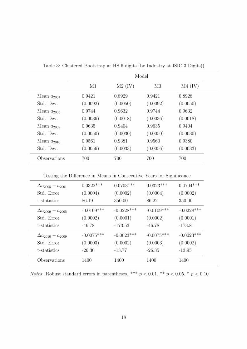
Table 3: Clustered Bootstrap at HS 6 digits (by Industry at ISIC 3 Digits))

Model

M1 M2 (IV) M3 M4 (IV)

Mean a2001 0.9421 0.8929 0.9421 0.8928

Std. Dev. (0.0092) (0.0050) (0.0092) (0.0050)

Mean a2005 0.9744 0.9632 0.9744 0.9632

Std. Dev. (0.0036) (0.0018) (0.0036) (0.0018)

Mean a2009 0.9635 0.9404 0.9635 0.9404

Std. Dev. (0.0050) (0.0030) (0.0050) (0.0030)

Mean a2010 0.9561 0.9381 0.9560 0.9380

Std. Dev. (0.0056) (0.0033) (0.0056) (0.0033)

Observations 700 700 700 700

Testing the Difference in Means in Consecutive Years for Significance

∆a2005 − a2001 0.0322*** 0.0703*** 0.0323*** 0.0704***

Std. Error (0.0004) (0.0002) (0.0004) (0.0002)

t-statistics 86.19 350.00 86.22 350.00

∆a2009 − a2005 -0.0109*** -0.0228*** -0.0109*** -0.0228***

Std. Error (0.0002) (0.0001) (0.0002) (0.0001)

t-statistics -46.78 -173.53 -46.78 -173.81

∆a2010 − a2009 -0.0075*** -0.0023*** -0.0075*** -0.0023***

Std. Error (0.0003) (0.0002) (0.0003) (0.0002)

t-statistics -26.30 -13.77 -26.35 -13.95

Observations 1400 1400 1400 1400

Notes : Robust standard errors in parentheses. *** p < 0.01, ** p < 0.05, * p < 0.10

18

tariffs. To do the median approach aggregation at 3-digit ISIC level does not make sense

as it will not be different from the simple mean ISIC 3 aggregation. By introducing such

an aggregation (simple mean at the 3-digits ISIC), the import tariff variation among

industries is further reduced. I estimate the same regressions presented in Equations 6

and 7. The results and trends remain robust. However, the values of the parameters “a”

go up for both models (the simple OLS and the IV Model) for all years. The Adjusted

R2 also increases. All those increases can be explained by the reduction of observations

due to the aggregation as well as by decrease in variation among the values of the left

hand side variable (as presented in Tables A.5 and A.6). The bootstrap results for the

3-digit ISIC import tariff aggregation are shown in Table A.8. The values of “a” and

the trend are robust. Therefore, one can reject the hypothesis that there is no change

of parameter “a” over time. Moreover, the result shows that the difference in “a” in

consecutive periods is again significant at 1 percent level.

5 More findings and analysis

Despite the change in parameter “a” over years does not seem to be large as indicated in

the lower section of Table 2, it is important to assess the quantitative significance of the

change in the welfare mindedness of the Russian government “a”. To do so, I calculate

the impact of this change on the average tariff level in Russia across all years of the

analysis. This calculation is based on Equation 4 and conducted by dividing the average

value of a variable in one year by the average value of the same variable in the previous

year, i.e. the value for the year 2005 is divided by the value in 2001. As there is no

variation in ei over years in my setting, this variable is eliminated:

tit1+titti(t−1)

1+ti(t−1)

=

(1−at)at

(1−a(t−1))

a(t−1)

∗yitmit

yi(t−1)

mi(t−1)

(9)

i = 1, ...n and time period t = 2001, 2005, 2009, 2010 and (t − 1) implies the previous

period.

Thus, if it had been a shift in the parameter “a” (from 0.8931 to 0.9631) alone, the

tariffs would have fallen as predicted by the PFS Model by around 57 percent (and by

19

Table 4: Quantitative Significance of Parameter “a” change over years

t/(1 + t) (1− a)/a (1− a)/a in IV Model yi/mi

2005/2001 0.9678 0.4283 0.3200 1.7328

2009/2005 0.9496 1.4350 1.6523 0.7985

2010/2009 0.9060 1.2196 1.0428 0.9265

68 percent in the IV Model) between 2001 and 2005. In fact one observes only about

3 percent average import tariff dercease in the Russian data set. Even more interesting

result is presented for the year pair 2009/2005 in Table 4. The decrease in parameter “a”

alone from 0.963 to 0.94 predicts import tariff increase by 43 percent (or by 65 percent in

the IV Model). However, one observes almost 5 percent average import tariff reduction

(not increase). With the creation of the Custom Union, as indicated in Table 2, there is

further decrease in the welfare mindedness of the government from 0.94 to 0.938, which

predicts an increase of the average import tariff level by 22 percent (or by 4 percent in

the IV Model). In fact, the data show a 10 percent decrease (not increase) of an average

import tariff level in 2010. This observation gives a sense of substantial quantitative

significance of the parameter change for the average protection level.

The critics, however, might point out that import tariffs were not the only forms of

protectionism which Russia used in 2009 and 2010. One could argue that the structure of

protection in the tariff schedule remains representative, i.e. the industries which are extra

protected by various commercial policy tools already have slightly higher import tariffs

in the tariff schedule. Therefore, to study the structure of protection using the import

tariff schedule is not wrong, but this approach might under-predict the actual level of

protection for certain industries. Moreover, it is important to remember that PFS model

was originally designed for import tariffs and subsidies only. Russia, however, used also

other forms of protection in 2009-2010 as stated in Gerasimenko (2012). Therefore, it is

appropriate to use Russian import tariff schedules to test the PFS model but at the same

time it is necessary to find a way to deal with the potential under-prediction of the actual

protection level, such as the residuals regression analysis demonstrated in the paper.

20

Another interesting observation is related to the Harmonized System (HS) classifica-

tions of import tariffs. Not only they are updated every four years at the UN level, the

regular changes are made at the 10-digit HS code by governments at home. Thus, in

order to bring down the average import tariff rate one creates “fake” import tariff lines

at the 10-digit HS level such as “other” and give them the import tariff value 0. On

paper, this manipulation brings an average import tariff level down, but de facto import

tariff can even go up for the particular good at interest. This trick was observed in the

Russian import tariff schedule as well. Those “average import tariff” manipulations are

well known in the trade policy world. Therefore, to work with the average import tariff

level, when the whole tariff schedule is included in analysis, might in fact under-predict

the actual (real) level of protection.

The next step is to conduct the residual regression analysis of the estimated models

(M1, M2, M3, M4) presented in Table 2 of this paper. I run residual analysis separately

for the import tariff schedule for December 2009 and for the Customs Union Import

tariff schedule of 2010 (valid from 1 January 2010). As shown in Table 5, the Russian

exports in 2008 are significant at 1 percent level in explaining residuals in all four models.

The variable “Number of protectionist measures other than import tariffs per industry”

(a proxy for the government attention to the industry) is significant at 1 percent level

as well as whether the Russian government has announced the industry to be a part

of its industrial policy programme (dummy variable “Announced Industrial policy”).

However, if I split the “Announced Industrial policy” variable into two more detailed other

dummy variables - “Announced modernization” and “Announced Import-Substitution”

(ISI), the results for 2009 import tariff schedule show positive significant (at 1 percent

level) results only for “Announced Import-Substitution” (ISI). This suggests that the

PFS model under-predicts tariff level where the Russian government has ISI policy in

mind. To rephrase it, the government uses other than import tariffs types of measures

to protect those industries. Indeed, this statement finds support in Gerasimenko (2012),

where a set of special industrial policy programmes for those industries is listed in the

appendix.

The Customs Union import tariff schedule residual regression analysis is presented in

Table 6. The question is why and in which way the presence of the Customs Union could

21

affect the residuals in Table 2 in 2010? Whether the interests of other CU members can

partly explain the residuals from the 2010 CU common import tariff schedule estimated

for Russia? Earlier in this paper, it was shown that all three countries had to adjust their

import tariff schedules of 2009 to different extent in order to implement the common ex-

ternal import tariff of the CU. The most serious adjustments (55 percent of its tariff lines)

were made by Kazakhstan. Moreover, from March 2010 Kazakhstan has also introduced

industrial policy strategy - “State Programme for the Accelerated Industrial Develop-

ment for 2010-2014”. This programme also identifies the priority industries, which are

supported by subsidies, export support measures, as well as import tariffs, and other non-

tariff measures. From October 2010, Kazakhstan has also announced “The Programme

for the Trade Development for 2010-2014”. Not surprisingly, the Kazakhstan’s exports

are significant in explaining the 2010 residuals for Russia. Also many experts would say

that the Customs Union import tariff schedule is mainly Russian import tariffs interests,

the finding suggests, however, that exports of Kazakhstan can partly explain the tariff

levels of the Customs Union (exports in this case are the proxy for the industrial policy

interests). The significant negative coefficient implies that the import tariff level in 2010

is slightly over-predicted where the Kazakh export interests are present. Belarus import

tariffs in 2009 were relatively more synchronized with the Russian import tariff schedule.

This explains why the Belorussian tariff adjustments for the 2010 CU common external

tariff did not need to be large (25 percent of tariff lines). Russia did import tariff adjust-

ments for 18 percent of its tariff lines in order to implement the CU common import tariff

schedule which is analyzed in the paper as the import tariff schedule of Russia for 2010.

“Announced Industrial Policy by Russia” variable is in 2010 again significant at 1 percent

level. However, if I split this variable into two as for the year 2009, than both, “Announced

modernization” and “Announced Import-Substitution” (ISI), are significant with positive

coefficients. This implies that in 2010 the PFS model under-predicts the tariff level of the

Customs Union schedule where the Russian Government has both modernization and ISI

policy in mind. Thus, the measures other than import tariffs are introduced to support

industries listed in those variables which is again in line with the findings presented in

Gerasimenko (2012). Indeed, in 2010 more measures were introduced for the industries

listed as priority industries for the modernization programme.

22

The low R2 for both, 2009 and 2010 regressions, suggests that there could be many

other factors which determine trade policy making such as foreign direct investments

(FDIs) per industry, internal investments, exchange rate manipulations and others.

The question for further research is whether the higher parameter “a” leads to eco-

nomic stability or the economic stability leads to higher welfare mindedness of the gov-

ernment. Theoretically the causality should work both ways, which implies that without

external shocks to the system the parameter “a” has impact on economic performance as

well as the economic performance has subsequent impact on the value of the parameter

“a”. However, if one looks at the role of the an external shock such as the global eco-

nomic crisis, then the argument could go this way: an external economic shock triggers

declining economic situation, that could lead to a decrease of the government welfare

mindedness (parameter ‘a”) simply by reflecting the needs of the problematic industries

during crisis (1-a)- it is the way the PFS model is designed. There could be, of course,

other explanations of the change in “a” such as the declining economic situation (without

external shock) or the socio-political differences of Medvedev and Putin regimes or all of

them at the same time. It would be interesting to look at this model in a yearly dynamics

if these data become available. Based on the results of this paper, one can state that

the value of welfare mindedness of government (parameter “a”) and economic situation

in the country could be correlated.

23

Table 5: Residual Analysis for the Year 2009 (Import Tariff Schedule from December 2009)

Model

M1 M1 M2 M2 M3 M3 M4 M4

Russian Export Value 2008 (in USD) -4.8E-11*** -4.3E-11*** -7.7E-11*** -7.1E-11*** -4.8E-11*** -4.3E-11*** -7.7E-11*** -7.1E-11***

(3.0E-12) (3.0E-12) (2.9E-12) (3.0E-12) (3.0E-12) (3.0E-12) (2.9E-12) (3.0E-12)

Nb. of Measures per Industry (from GTA) -0.03076*** -0.0200*** -0.0254*** -0.0138** -0.0302*** -0.0196*** -0.0249*** -0.0133*

(0.0065) (0.0067) (0.0066) (0.0070) (0.0066) (0.0068) (0.0067) (0.0070)

Reference: Announced Industrial Policy (Not)

Announced Industrial Policy (Yes) 0.5169*** 0.5804*** 0.5186*** 0.5823***

(0.0577) (0.0593) (0.0578) (0.0594)

Announced Modernization 0.0874 0.1124 0.0906 0.1156

(0.0660) (0.0826) (0.0663) (0.0828)

Announced Import-Substitution (ISI) 0.6466*** 0.7219*** 0.6479*** 0.7233***

(0.0695) (0.0704) (0.0696) (0.0704)

Constant 0.3628*** 0.3084*** 0.1702*** 0.1110** 0.3606*** 0.3064*** 0.1677*** 0.1086**

(0.0503) (0.0518) (0.0520) (0.0540) (0.0506) (0.0521) (0.0524) (0.0543)

Observations 3938 3938 3938 3938 3938 3938 3938 3938

R2 0.0347 0.0415 0.0434 0.0510 0.0346 0.0413 0.0434 0.0508


24

Table 6: Residual Analysis for the Year 2010 (Customs Union Schedule from April 2010)

Model

M1 M1 M2 M2 M3 M3 M4 M4

Russian Export Value 2009 (in USD) -1.2E-10 -1.2E-10 -1.9E-10 -2.0E-10 -1.4E-10 -1.4E-10 -2.1E-10 -2.2E-10

(3.1E-10) (3.1E-10) (3.2E-10) (3.1E-10) (3.2E-10) (3.2E-10) (3.2E-10) (3.2E-10)

Nb. of Measures per Industry (from GTA) -0.0166*** -0.0079 -0.0148** -0.0059 -0.0163*** -0.0076 -0.0145** -0.0056

(0.0059 ) (0.0064) (0.0060) (0.0065) (0.0059) (0.0064) (0.0060) (0.0065)

Reference: Announced Industrial Policy (Not)

Announced Industrial Policy (Yes) 0.4494*** 0.4970*** 0.4502*** 0.4980***

(0.0546 ) (0.0553) (0.0547) (0.0553)

Announced Modernization 0.0981* 0.1383** 0.0963* 0.1366**

(0.0578) (0.0646) (0.0577) (0.0645)

Announced Import-Substitution (ISI) 0.5611*** 0.6111*** 0.5627*** 0.6128***

(0.0684) (0.0687) (0.0684) (0.0688)

Belarus Export Value 2009 (in USD) 1.7E-09 1.7E-09 1.9E-09 1.9E-09 1.6E-09 1.6E-09 1.8E-09 1.9E-09

(2.2E-09) (2.2E-09) (2.2E-09) (2.2E-09) (2.3E-09) (2.3E-09) (2.2E-09) (2.2E-09)

Kazakhstan Export Value 2009 (in USD) -1.4E-09** -1.4E-09** -1.7E-09** -1.7E-09** -1.4E-09** -1.4E-09** -1.7E-09** -1.7E-09**

(6.6E-10) (6.6E-10) (8.0E-10) (8.0E-10) (6.7E-10) (6.7E-10) (8.1E-10) (8.1E-10)

Belarus Import Value 2009 (in USD) -5.3E-09 -4.9E-09 -4.4E-09 -4.0E-09 -4.3E-09 -3.9E-09 -3.5E-09 -3.1E-09

(3.5E-09) (3.5E-09) (3.4E-09) (3.4E-09) (4.1E-09) (4.1E-09) (4.1E-09) (4.1E-09)

Kazakhstan Import Value 2009 (USD) -8.5E-10 -7.2E-10 -9.2E-10 -7.8E-10 -9.3E-10 -8.0E-10 -1.0E-09 -8.6E-10

(5.9E-10) (5.3E-10) (6.3E-10) (5.7E-10) (6.9E-10) (6.3E-10) (7.2E-10) (6.6E-10)

Constant 0.2509*** 0.2047*** 0.1200*** 0.0729 0.2473*** 0.2008*** 0.1161** 0.0686

(0.0455) (0.0478) (0.0463) (0.0488) (0.0464) (0.0486) (0.0472) (0.0496)

Observations 3959 3959 3959 3959 3959 3959 3959 3959

R2 0.0318 0.0374 0.0383 0.0438 0.0312 0.0368 0.0378 0.0434


25

6 Conclusion

In this paper the estimation of the determinants of trade policy making are closely guided

by the theoretical model presented by Grossman and Helpman (1994). There is a couple

of benefits to follow this path. First, it allows to empirically examine the existing model of

trade policy making in other than western democratic settings and in the shock conditions

such as global economic crisis. Second, it allows to estimate the structural parameter “a”

in dynamics (2001, 2005, 2009, and 2010) over the same political leadership which can

contain interesting information about government priorities over time and particular in

a crisis.

I used two econometric model specifications to estimate the welfare mindedness (pa-

rameter “a”) of the Russian government during the recent crisis. The data used for this

paper contains import tariffs and industry specific information for 2001, 2005, 2009, and

2010. I find that the pattern of protection in the Russian Federation in 2001, 2005, 2009

and 2010 is in line with the predictions of the model, i.e. protection to organized sectors is

negatively related to import penetration. Both econometric model specifications showed

the same trend - positive highly significant values of the parameter β which were used

to calculate the value of welfare mindedness of the Russian government “a” for all four

years.

The government weight on welfare in the government’s objective function is larger

than the weight on contributions across all years of analysis that is in compliance with

the findings in the existing literature on this subject. Then, I compare the estimation

results in stability times (2005) as well as during the hard phase of anti-crisis policy in

2009 and the rapid creation of the Customs Union of Russia, Belarus and Kazakhstan

in 2010. The welfare mindedness of the Russian government in the crisis is estimated

to be smaller relatively to the economic stability times. To rephrase this statement,

the weight that government puts on contributions from lobbies increased during crisis

relatively to non-crisis times. This might be driven by intensified lobbying activities by

industries or firms to get state support in the times of financial difficulty and falling

demand. Thus, Russia, not being bound by the WTO commitments neither by the

WTO accession process in 2009-2010, had the widest range of possible commercial policy

26

moves. It actively used import tariff modifications as the anti-crisis management and even

industrial policy tools. The result of 2001 vs. 2005 only supports the earlier mentioned

argument. The welfare mindedness of the Russian government in 2001 was determined

by the anti-crisis management of the Russian 1998 economic crisis as well as by the

rapid development of the Russian domestic import substituting industries (especially

food industry).

Despite the change in the parameter “a” over years does not seem large, it has a

substantial quantitative effect on the average import tariff level (if it would be a shift in the

parameter “a” alone). Moreover, the residual regression analysis shows that the import

tariff level is under-predicted for those industries where the government has industrial

policy in mind implying that there should be other than import tariff measures used by

the government, which is in line with the findings in Gerasimenko (2012). The industrial

policy interests of other members of the Customs Union can also partly explain the

residuals from the PFS model estimation for 2010.

There could be other than global economic crisis reasons explaining the down- sloping

shift in parameter “a” during crisis such as the worsening domestic economic situation

(independently of the global crisis), political changes and others. However, it is hard

to argue that the latest global crisis to a different extent impacted all economies in a

negative way, which I argue led governments to focus on proving protection in various

forms to the industries and firms in need. This implies, in the way the “Protection for

sale” model and its government utility function are designed, that a government puts

more weight on contributions (1-a) and as a consequence, less weight on the welfare of

society (parameter “a”).

One could argue that this trend (increasing weight on lobbyist contributions in crisis

relative to economic stability times) could also be found among other countries if it would

be possible to transfer the Global Trade Alert data on anti-crisis trade policies into import

the tariff ad-valorem equivalents and test the PFS model across countries. The literature

mentioned above makes a qualitative assessment of the patterns of trade policy making

in the crisis around the world. This research finds government selectivity patterns among

industries and firms who got support during recent economic downturn. This qualitative

observation could find support in the quantitative assessment of “a” across countries over

27

time.

References

Aggarwal, V. and S. J. Evenett (2012): “Industrial policy choice during the crisis

era,” Oxford Review of Economic Policy, Summer 28, 261–283.

Baldwin, R. and S. J. Evenett (2012): “Beggar-thy-neighbour policies during the

crisis era: causes, constraints, and lessons for maintaining open borders,” Oxford Re-

view of Economic Policy, Summer 28, 211–234.

Evans, C. L. and S. M. Sherlund (2011): “Are Antidumping Duties for Sale? Case-

Level Evidence on the Grossman-Helpman Protection for Sale Model,” Southern Eco-

nomic Journal, 78, 330–357.

Evenett, S. J. (2011): “Did WTO Rules Restrain Protectionism During the Recent

Systemic Crisis?” Discussion Paper 8687, Center for Economic Policy Reseach (CEPR),

London.

Evenett, S. J., J. Fritz, D. Gerasimenko, M. Nowakowska, and M. Wer-

melinger (2011): “The Resort to Protectionism During the Great Recession: Which

Factors Mattered?” Working paper, University of St. Gallen.

Gawande, K. and U. Bandyopadhyaya (2000): “Is Protection for Sale? Evidence of

the Grossman-Helpman Theory of Endogenous Protection,” The Review of Economics

and Statistics, 82, 139–152.

Gawande, K., K. Pravin, and M. Olarreaga (2009): “What Governments Maxi-

mize and Why: The View from Trade,” International Organization, 491–532.

——— (2012): “Lobbying Competition over Trade Policy,” International Economic Re-

view, 53, 115–132.

Gerasimenko, D. (2012): “Russia’s commercial policy, 2008-11: modernization, crisis,

and the WTO accession,” Oxford Review of Economic Policy, Summer 28, 301–323.

28

Goldberg, P. K. and G. Maggi (1999): “Protection for Sale: An Empirical Investi-

gation,” American Economic Review, 89, 1135–1155.

Grossman, G. and E. Helpman (1994): “Protection for Sale,” American Economic

Review, 84, 833–850.

Kee, H. L., C. Neagu, and A. Nicita (2013): “Is Protectionism on the Rise? As-

sessing National Trade Policies during the Crisis of 2008,” The Review of Economics

and Statistics, 95, 342–346.

Kee, H. L., A. Nicita, and M. Olarreaga (2008): “Import Demand Elasticities

and Trade Distortions,” The Review of Economics and Statistics, 90, 666–682.

McCalman, P. (2004): “Protection for Sale and Trade Liberalization: an Empirical

Investigation,” Review of International Economics, 12, 81–94.

Mitra, D., D. Thomakos, and M. Ulubasoglu (2002): “”Protection for Sale” in

a Developing Country: Democracy vs. Dictatorship,” The Review of Economics and

Statistics, 84, 497–508.

Trefler, D. (1993): “Trade Liberalization and the Theory of Endogenous Protection,”

Journal of Political Economy, 101, 138–160.

A Appendix

The List of Variables Used in this paper and their sources:

1. Russian Import Tariff (ti) for 2001 at the 10-digit Harmonized System (HS) is taken

from Tariff Analysis Online facility provided by World Trade Organization (WTO). It is

aggregated by the author by simple average (as well as by median) to the 6-digit level

HS code.

2. Russian Import Tariff (ti) for 2005, 2009, 2010 is from the official legal documents

at the 10-digit HS code. It is aggregated by the author by simple average (as well as by

median) to the 6-digit level HS code.

29

3. Russian Imports value (mi) for 2001, 2005, 2009, 2010 is from the United Nations

Comtrade database at the 6-digit level HS code in current US dollars and aggregated to

the 3-digit ISIC Revision 3 code.

4. Domestic output per industry (yi) is available from Industrial Statistics Database

(INDSTAT4 - 2013 edition) at the 3-digit ISIC Revision 3 code for 2001, 2005, 2009 and

2010 in current US dollars.

5. The inverse import penetration ratio ( yimi

) is the value of domestic output per

industry divided by the value of total imports. It is calculated for 2001, 2005, 2009 and

2010 in current US dollars using the variables above.

6. The import demand elasticity (ei) is taken from Kee et al. (2008). The data is

available for Russia at the 6-digit level HS code from the website of the World Bank. It

is calculated there over 1988-2001 for 117 countries. As it is the only import demand

elasticity calculated for Russia I use it for all years in the analysis.

7. The political organization dummies (Ii = 1) for all 57 manufacturing industries at

the 3-digit level ISIC code Revision 3.

8. Number of employees per industry for 2001, 2005, 2009 and 2010 is from UNIDO


Revision 3.

9. Total Wages per industry for 2001, 2005, 2009 and 2010 are from UNIDO Industrial

Statistics Database (INDSTAT4 - 2013 edition) at the 3-digit level of ISIC Revision 3 in

current US dollars.

10. Total Value added per industry for 2001, 2005, 2009 and 2010 is from UNIDO


Revision 3 in current US dollars.

11. Russian Export value for 2008, 2009 is from United Nations Comtrade database

at the 6-digit level HS code in current US dollars.

12. Belarus and Kazakhstan Exports and Imports value for 2009 is from United

Nations Comtrade database at the 6-digit level HS code in current US dollars.

13. “Nb. of protectionist (red) measures” other than import tariffs per industry (CPC

coding)in Russia for 2009-2010 are collected from the various legal documents (a part of

the GTA database).

30

14. “Announced Industrial Policy” is a dummy variable (Yes/No) constructed at 4-

digits ISIC level by the author based on the legal documents and Global Trade Alert

(GTA) database listed in Gerasimenko (2012)- whether the industry was announced as

an priority industry in the government programmes in 2008-2009. This variable is subdi-

vided into “Announced Modernization” and “Announced Import Substitution Industri-

alization”.

15. “Announced Modernization” is a dummy variable (Yes/No) constructed by the

author based on the information in Gerasimenko (2012). Those are the industries which

were announced as “perspective” from the modernization point of view.

16. “Announced Import Substitution” is a dummy variable (Yes/No) constructed by

the author based on the information in Gerasimenko (2012). Those are the industries

which were announced as “perspective” from the point of view of the import substitution

strategy.

31

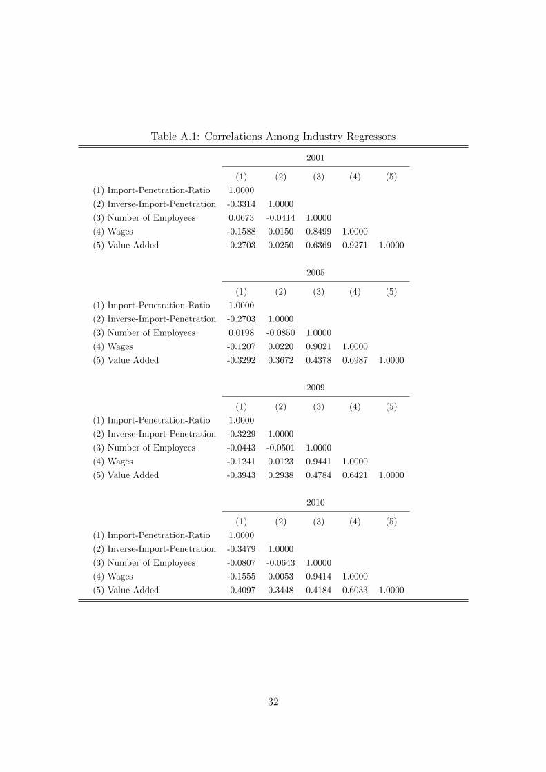
Table A.1: Correlations Among Industry Regressors

2001

(1) (2) (3) (4) (5)

(1) Import-Penetration-Ratio 1.0000

(2) Inverse-Import-Penetration -0.3314 1.0000

(3) Number of Employees 0.0673 -0.0414 1.0000

(4) Wages -0.1588 0.0150 0.8499 1.0000

(5) Value Added -0.2703 0.0250 0.6369 0.9271 1.0000

2005

(1) (2) (3) (4) (5)



(3) Number of Employees 0.0198 -0.0850 1.0000

(4) Wages -0.1207 0.0220 0.9021 1.0000

(5) Value Added -0.3292 0.3672 0.4378 0.6987 1.0000

2009

(1) (2) (3) (4) (5)



(3) Number of Employees -0.0443 -0.0501 1.0000

(4) Wages -0.1241 0.0123 0.9441 1.0000

(5) Value Added -0.3943 0.2938 0.4784 0.6421 1.0000

2010

(1) (2) (3) (4) (5)



(3) Number of Employees -0.0807 -0.0643 1.0000

(4) Wages -0.1555 0.0053 0.9414 1.0000

(5) Value Added -0.4097 0.3448 0.4184 0.6033 1.0000

32

Table A.2: Correlations among “Protection for Sale”- Model Variables

2001

(1) (2) (3)

(1) Tariff (6-Digits-Level) 1.0000

(2) Abs. Import-Demand-Elasticity (e) 0.0166 1.0000

(3) Import Penetration Ratio (m/y) 0.0124 -0.0349 1.0000

2005

(1) (2) (3)



(3) Import Penetration Ratio (m/y) -0.1153 -0.0921 1.0000

2009

(1) (2) (3)




2010

(1) (2) (3)




33

Table A.3: Regression Results with Standard Errors at HS 6 digits level

Model

M1 M2 (IV) M3 M4 (IV)

β2001 0.0617*** 0.1197*** 0.0618*** 0.1199***

(0.0033) (0.0082) (0.0033) (0.0082)

t-statistics 18.79 14.57 18.79 14.58

Adj.R2 0.0780 na 0.0780 na

Observations 4164 4164 4164 4164

β2005 0.0265*** 0.0383**** 0.0266*** 0.0383***

(0.0017) (0.0026) (0.0017) (0.0026)

t-statistics 15.85 14.79 15.84 14.77

Adj.R2 0.0577 na 0.0576 na

Observations 4085 4085 4085 4085

β2009 0.0381*** 0.0633*** 0.0381*** 0.0634***

(0.0021) (0.0040) (0.0021) (0.0040)

t-statistics 17.75 15.90 17.74 15.89

Adj.R2 0.0739 na 0.0738 na

Observations 3938 3938 3938 3938

β2010 0.0465*** 0.0660*** 0.0465*** 0.0661***

(0.0024) (0.0039) (0.0024) (0.0039)

t-statistics 19.55 16.78 19.53 16.77

Adj.R2 0.0878 na 0.0877 na

Observations 3959 3959 3959 3959


a2001 0.9419 0.8931 0.9418 0.8929

a2005 0.9741 0.9631 0.9741 0.9631

a2009 0.9633 0.9405 0.9633 0.9404

a2010 0.9556 0.9381 0.9555 0.9380

Notes: Standard errors in parentheses. *** p < 0.01, ** p < 0.05, * p < 0.10

34

Table A.4: Bootstrap at HS 6 digits Tariff Level

Model

M1 M2 (IV) M3 M4 (IV)

Mean a2001 0.9414 0.8929 0.9414 0.8928

Std. Dev. (0.0101) (0.0051) (0.0101) (0.0051)

Mean a2005 0.9741 0.9628 0.9741 0.9628

Std. Dev. (0.0046) (0.0055) (0.0046) (0.0055)

Mean a2009 0.9630 0.9400 0.9629 0.9400

Std. Dev. (0.0053) (0.0059) (0.0053) (0.0059)

Mean a2010 0.9554 0.9378 0.9553 0.9377

Std. Dev. (0.0061) (0.0046) (0.0061) (0.0047)

Observations 700 700 700 700


∆a2005 − a2001 0.0327*** 0.0699*** 0.0327*** 0.0700***

Std. Error (0.0004) (0.0003) (0.0004) (0.0003)

t-statistics 77.91 250.00 77.91 250.00

∆a2009 − a2005 -0.0111*** -0.0228*** -0.0111*** -0.0228***

Std. Error (0.0003) (0.0003) (0.0003) (0.0003)

t-statistics -41.86 -74.96 -41.85 -74.99

∆a2010 − a2009 -0.0076*** -0.0022*** -0.0076*** -0.0023***

Std. Error (0.0003) (0.0003) (0.0003) (0.0003)

t-statistics -24.94 -7.94 -24.98 -8.03

Observations 1400 1400 1400 1400


35

Table A.5: Russian Mean Tariff Rate at ISIC 3 level of aggregation (1/2)

ISIC Description 2001 2005 2009 2010

151 Production, processing of meat, fish, fruit,etc. 12.83 13.90 15.05 15.84

152 Man. dairy products 13.67 13.51 13.67 14.53

153 Man. grain mill products 9.48 11.37 11.50 11.50

154 Man. other food products 13.41 12.13 12.14 13.26

155 Man. beverages 27.67 27.00 27.00 27.00

160 Man. tobacco products 25.00 22.78 22.78 22.78

171 Spinning, weaving and finishing of textiles 10.57 10.63 10.58 9.56

172 Man. other textiles 15.18 15.18 14.95 14.41

173 Man. knitted and crocheted fabrics 13.05 11.98 11.96 10.58

181 Man. wearing apparel, except fur apparel 19.84 19.83 19.81 10.24

182 Dressing and dyeing of fur 12.17 12.44 11.66 11.21

191 Tanning and dressing of leather 10.71 9.90 9.26 8.97

192 Manufacture of footwear 14.31 14.31 10.58 8.37

201 Sawmilling and planing of wood 15.00 15.00 15.00 15.00

202 Manufacture of products of wood, cork,etc. 14.93 14.64 15.40 14.55

210 Man. paper and paper products 13.49 13.59 13.49 12.71

221 Publishing 8.84 8.66 4.45 4.45

222 Printing and service activities related to it 13.89 13.89 13.33 13.33

231 Man. coke oven products 5.00 5.00 5.00 5.00

232 Man. refined petroleum products 5.00 4.99 4.84 4.84

233 Processing of nuclear fuel 7.00 7.00 5.67 5.67

241 Man. basic chemicals 6.01 5.97 5.91 5.76

242 Man. other chemical products 7.95 8.08 7.98 6.97

243 Man. man-made fibres 8.59 8.58 8.46 8.69

251 Man. rubber products 8.79 8.57 8.31 7.51

252 Man. plastics products 13.59 13.09 12.75 11.97

261 Man. glass and glass products 14.25 13.70 13.44 13.23

269 Man. non-metallic mineral products n.e.c 14.08 13.82 13.77 13.39

271 Man. basic iron and steel 6.87 6.81 6.72 7.79

272 Man. basic precious and non-ferrous metals 11.00 11.32 11.02 10.13

281 Man. structural metal products, tanks, etc. 12.88 12.88 12.24 11.18

289 Man. other fabricated metal products 13.11 12.87 12.41 11.60

291 Man. general purpose machinery 9.93 8.26 5.44 3.74

292 Man. special purpose machinery 8.90 7.06 4.54 3.37

293 Man. domestic appliances n.e.c. 14.40 14.15 14.02 10.24

300 Man. office, accounting and computing machinery 9.63 8.17 4.93 4.01

311 Man. electric motors, generators and transformers 9.06 8.16 4.99 4.71

312 Man. electricity distribution and control apparatus 12.89 11.28 10.29 10.29

313 Man. insulated wire and cable 17.50 15.42 14.17 14.17

314 Man. accumulators, primary cells and batteries 10.57 10.48 9.87 7.01

315 Man. electric lamps and lighting equipment 16.38 14.72 14.54 13.49

319 Man. other electrical equipment n.e.c. 10.48 9.51 7.51 6.70

36

Table A.6: Russian Mean Tariff Rate at ISIC 3 level of aggregation (2/2)

ISIC Description 2001 2005 2009 2010

321 Man. electronic valves and tubes, etc. 13.98 7.48 6.91 6.88

322 Man. television and radio transmitters 7.46 6.14 6.66 6.09

323 Man. television and radio receivers, etc. 17.47 12.44 11.84 9.93

331 Man. medical appliances and instruments 7.95 6.87 4.49 4.05

332 Man. optical instr. and photo. equipment 10.42 10.42 9.71 7.68

333 Man. watches and clocks 19.17 19.10 19.00 16.55

341 Man. motor vehicles 12.43 11.92 15.62 14.99

342 Man. bodies (coachwork) for motor vehicles 12.81 12.29 12.32 12.11

343 Man. parts and accessories for motor vehicles 5.29 2.89 2.06 2.07

351 Building and repairing of ships and boats 12.27 11.76 11.47 10.69

352 Man. railway and tramway locomotives 7.61 7.61 7.01 7.01

353 Man. aircraft and spacecraft 14.09 14.24 11.75 10.75

359 Man. transport equipment n.e.c. 12.25 12.25 10.71 10.50

361 Man. furniture 20.00 19.48 17.60 13.65

369 Manufacturing n.e.c. 16.23 16.16 16.13 13.28

37

Table A.7: Regression Results - Tariff Aggregation at ISIC 3 level

Model (M1) IV-Model (M2)

β2001 0.04247*** 0.0911***

Std. Error (0.004038) (0.0353)

t-statistics 10.52 2.58

Adj.R2 0.7045 na

Obs. 46 44

β2005 0.01737*** 0.0096**

Std. Error (0.00348) (0.0048)


Adj.R2 0.3799 na

Obs. 39 38

β2009 0.02790*** 0.0224***

Std. Error (0.00404) (0.0067)


Adj.R2 0.5449 na

Obs. 39 38

β2010 0.0303*** 0.0660***

Std. Error (0.0042) (0.0074)


Adj.R2 0.6473 na

Obs. 39 39


a2001 0.9593 0.9165

a2005 0.9829 0.9905

a2009 0.9729 0.9781

a2010 0.9654 0.9706


38

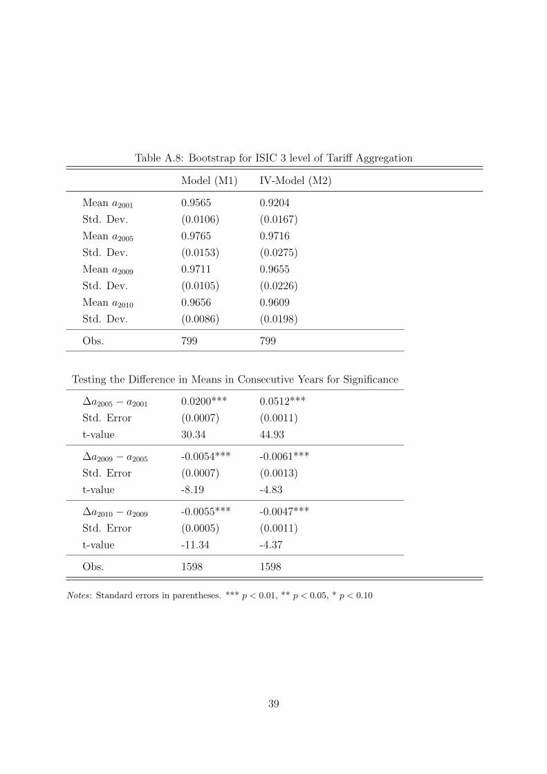
Table A.8: Bootstrap for ISIC 3 level of Tariff Aggregation

Model (M1) IV-Model (M2)

Mean a2001 0.9565 0.9204

Std. Dev. (0.0106) (0.0167)

Mean a2005 0.9765 0.9716

Std. Dev. (0.0153) (0.0275)

Mean a2009 0.9711 0.9655

Std. Dev. (0.0105) (0.0226)

Mean a2010 0.9656 0.9609

Std. Dev. (0.0086) (0.0198)

Obs. 799 799


∆a2005 − a2001 0.0200*** 0.0512***

Std. Error (0.0007) (0.0011)

t-value 30.34 44.93

∆a2009 − a2005 -0.0054*** -0.0061***

Std. Error (0.0007) (0.0013)

t-value -8.19 -4.83

∆a2010 − a2009 -0.0055*** -0.0047***

Std. Error (0.0005) (0.0011)

t-value -11.34 -4.37

Obs. 1598 1598


39

protection for sale di er in crisis vs. economic stability ... · does \protection for sale"...

Documents