provided for non-commercial research and educational use ...€¦ · adaptive filters vítor h....
TRANSCRIPT

Provided for non-commercial research and educational use only.Not for reproduction, distribution or commercial use.
This chapter was originally published in the book Academic Press Library in Signal Processing. The copyattached is provided by Elsevier for the author’s benefit and for the benefit of the author’s institution, for non-
commercial research, and educational use. This includes without limitation use in instruction at your institution,distribution to specific colleagues, and providing a copy to your institution’s administrator.
All other uses, reproduction and distribution, including without limitation commercial reprints, selling orlicensing copies or access, or posting on open internet sites, your personal or institution’s website or repository,
are prohibited. For exceptions, permission may be sought for such use through Elsevier's permissions site at:http://www.elsevier.com/locate/permissionusematerial
From Vítor H. Nascimento and Magno T. M. Silva, Adaptive Filters. In: Rama Chellappa, Sergios Theodoridis,editors, Academic Press Library in Signal Processing. Vol 1, Signal Processing Theory and Machine Learning,
Chennai: Academic Press, 2014, p. 619-761.ISBN: 978-0-12-396502-8
© Copyright 2014 Elsevier LtdAcademic Press.
Author’s personal copy
12CHAPTER
Adaptive Filters
Vítor H. Nascimento and Magno T. M. SilvaDepartment of Electronic Systems Engineering, University of São Paulo, São Paulo, SP, Brazil
1.12.1 IntroductionAdaptive filters are employed in situations in which the environment is constantly changing, so that afixed system would not have adequate performance. As they are usually applied in real-time applications,they must be based on algorithms that require a small number of computations per input sample.
These algorithms can be understood in two complementary ways. The most straightforward wayfollows directly from their name: an adaptive filter uses information from the environment and fromthe very signal it is processing to change itself, so as to optimally perform its task. The informationfrom the environment may be sensed in real time (in the form of a so-called desired signal), or may beprovided a priori, in the form of previous knowledge of the statistical properties of the input signal (asin blind equalization).
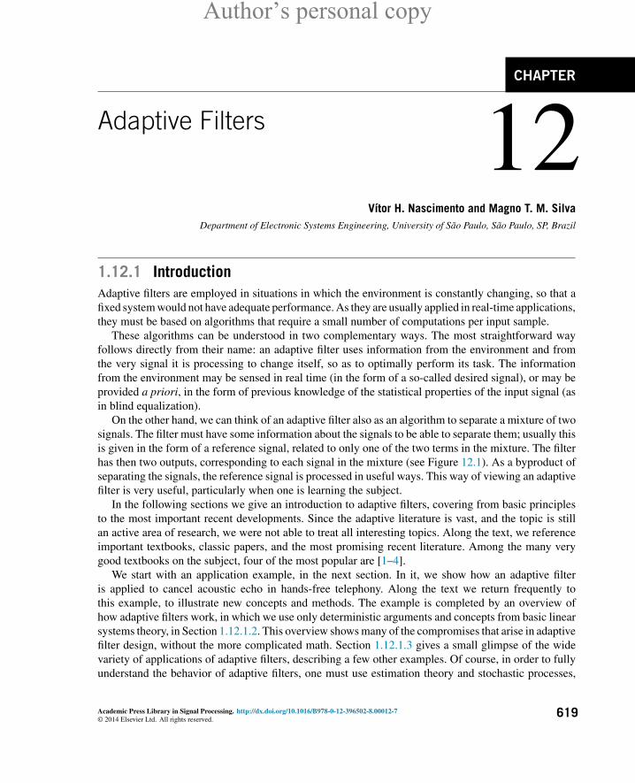
On the other hand, we can think of an adaptive filter also as an algorithm to separate a mixture of twosignals. The filter must have some information about the signals to be able to separate them; usually thisis given in the form of a reference signal, related to only one of the two terms in the mixture. The filterhas then two outputs, corresponding to each signal in the mixture (see Figure 12.1). As a byproduct ofseparating the signals, the reference signal is processed in useful ways. This way of viewing an adaptivefilter is very useful, particularly when one is learning the subject.
In the following sections we give an introduction to adaptive filters, covering from basic principlesto the most important recent developments. Since the adaptive literature is vast, and the topic is stillan active area of research, we were not able to treat all interesting topics. Along the text, we referenceimportant textbooks, classic papers, and the most promising recent literature. Among the many verygood textbooks on the subject, four of the most popular are [1–4].
We start with an application example, in the next section. In it, we show how an adaptive filteris applied to cancel acoustic echo in hands-free telephony. Along the text we return frequently tothis example, to illustrate new concepts and methods. The example is completed by an overview ofhow adaptive filters work, in which we use only deterministic arguments and concepts from basic linearsystems theory, in Section 1.12.1.2. This overview shows many of the compromises that arise in adaptivefilter design, without the more complicated math. Section 1.12.1.3 gives a small glimpse of the widevariety of applications of adaptive filters, describing a few other examples. Of course, in order to fullyunderstand the behavior of adaptive filters, one must use estimation theory and stochastic processes,
Academic Press Library in Signal Processing. http://dx.doi.org/10.1016/B978-0-12-396502-8.00012-7© 2014 Elsevier Ltd. All rights reserved.
619
Author’s personal copy620 CHAPTER 12 Adaptive Filters
adaptivefilter
Mixture of signals
Output 2 (“error”signal)
Reference signal Output 1
d1(n)
y1(n)
x1(n)
e1(n)Adaptation
Algorithm
Filter
Adaptive filter
FIGURE 12.1
Inputs and outputs of an adaptive filter. Left: detailed diagram showing inputs, outputs and internal variable.Right: simplified diagram.
which is the subject of Sections 1.12.2 and 1.12.3. The remaining sections are devoted to extensions tothe basic algorithms and recent results.
Adaptive filter theory brings together results from several fields: signal processing, matrix analysis,control and systems theory, stochastic processes, and optimization. We tried to provide short reviewsfor most of the necessary material in separate links (“boxes”), that the reader may follow if needed.
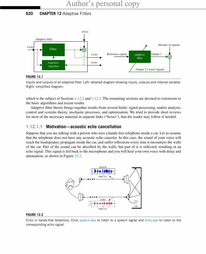
1.12.1.1 Motivation—acoustic echo cancellationSuppose that you are talking with a person who uses a hands-free telephone inside a car. Let us assumethat the telephone does not have any acoustic echo canceler. In this case, the sound of your voice willreach the loudspeaker, propagate inside the car, and suffer reflections every time it encounters the wallsof the car. Part of the sound can be absorbed by the walls, but part of it is reflected, resulting in anecho signal. This signal is fed back to the microphone and you will hear your own voice with delay andattenuation, as shown in Figure 12.2.
car
speech
echo
time (s)
time (s)
1
1
1
2
2
3
3
4
4-1
0
0
0
0
-0.2
0.2
FIGURE 12.2
Echo in hands-free telephony. Click speech.wav to listen to a speech signal and echo.wav to listen to thecorresponding echo signal.
Author’s personal copy1.12.1 Introduction 621
adaptivefilter
car
speech
echo
time (s)
time (s)
1
1
1
2
2
3
3
4
4-1
0
0
0
0
-0.2
0.2
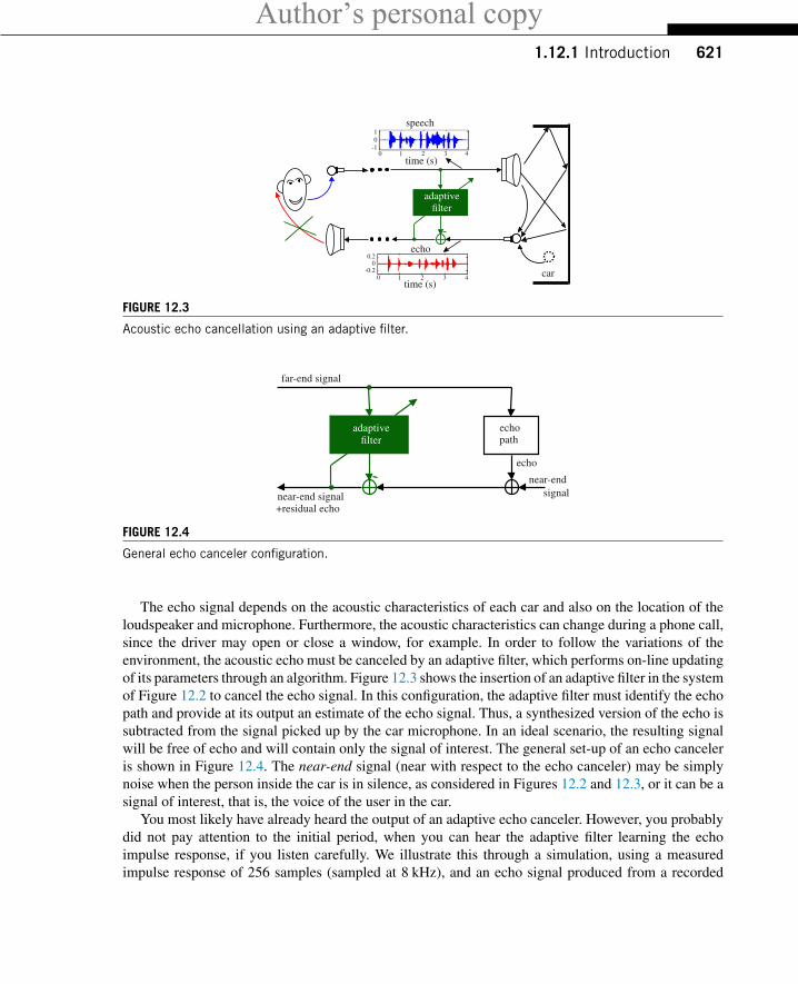
FIGURE 12.3
Acoustic echo cancellation using an adaptive filter.
adaptivefilter
signal
+residual echo
echo
echo
near-end signal
near-end
path
far-end signal
FIGURE 12.4
General echo canceler configuration.
The echo signal depends on the acoustic characteristics of each car and also on the location of theloudspeaker and microphone. Furthermore, the acoustic characteristics can change during a phone call,since the driver may open or close a window, for example. In order to follow the variations of theenvironment, the acoustic echo must be canceled by an adaptive filter, which performs on-line updatingof its parameters through an algorithm. Figure 12.3 shows the insertion of an adaptive filter in the systemof Figure 12.2 to cancel the echo signal. In this configuration, the adaptive filter must identify the echopath and provide at its output an estimate of the echo signal. Thus, a synthesized version of the echo issubtracted from the signal picked up by the car microphone. In an ideal scenario, the resulting signalwill be free of echo and will contain only the signal of interest. The general set-up of an echo canceleris shown in Figure 12.4. The near-end signal (near with respect to the echo canceler) may be simplynoise when the person inside the car is in silence, as considered in Figures 12.2 and 12.3, or it can be asignal of interest, that is, the voice of the user in the car.
You most likely have already heard the output of an adaptive echo canceler. However, you probablydid not pay attention to the initial period, when you can hear the adaptive filter learning the echoimpulse response, if you listen carefully. We illustrate this through a simulation, using a measuredimpulse response of 256 samples (sampled at 8 kHz), and an echo signal produced from a recorded
Author’s personal copy622 CHAPTER 12 Adaptive Filters
−0.03
−0.02
−0.01
0.01
0.02
0.03
0
0 10 20 30time (ms)
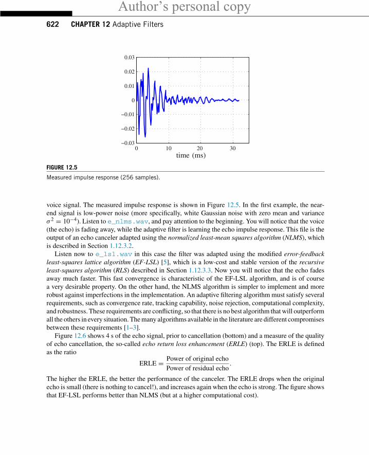
FIGURE 12.5
Measured impulse response (256 samples).
voice signal. The measured impulse response is shown in Figure 12.5. In the first example, the near-end signal is low-power noise (more specifically, white Gaussian noise with zero mean and varianceσ 2 = 10−4). Listen to e_nlms.wav, and pay attention to the beginning. You will notice that the voice(the echo) is fading away, while the adaptive filter is learning the echo impulse response. This file is theoutput of an echo canceler adapted using the normalized least-mean squares algorithm (NLMS), whichis described in Section 1.12.3.2.
Listen now to e_lsl.wav in this case the filter was adapted using the modified error-feedbackleast-squares lattice algorithm (EF-LSL) [5], which is a low-cost and stable version of the recursiveleast-squares algorithm (RLS) described in Section 1.12.3.3. Now you will notice that the echo fadesaway much faster. This fast convergence is characteristic of the EF-LSL algorithm, and is of coursea very desirable property. On the other hand, the NLMS algorithm is simpler to implement and morerobust against imperfections in the implementation. An adaptive filtering algorithm must satisfy severalrequirements, such as convergence rate, tracking capability, noise rejection, computational complexity,and robustness. These requirements are conflicting, so that there is no best algorithm that will outperformall the others in every situation. The many algorithms available in the literature are different compromisesbetween these requirements [1–3].
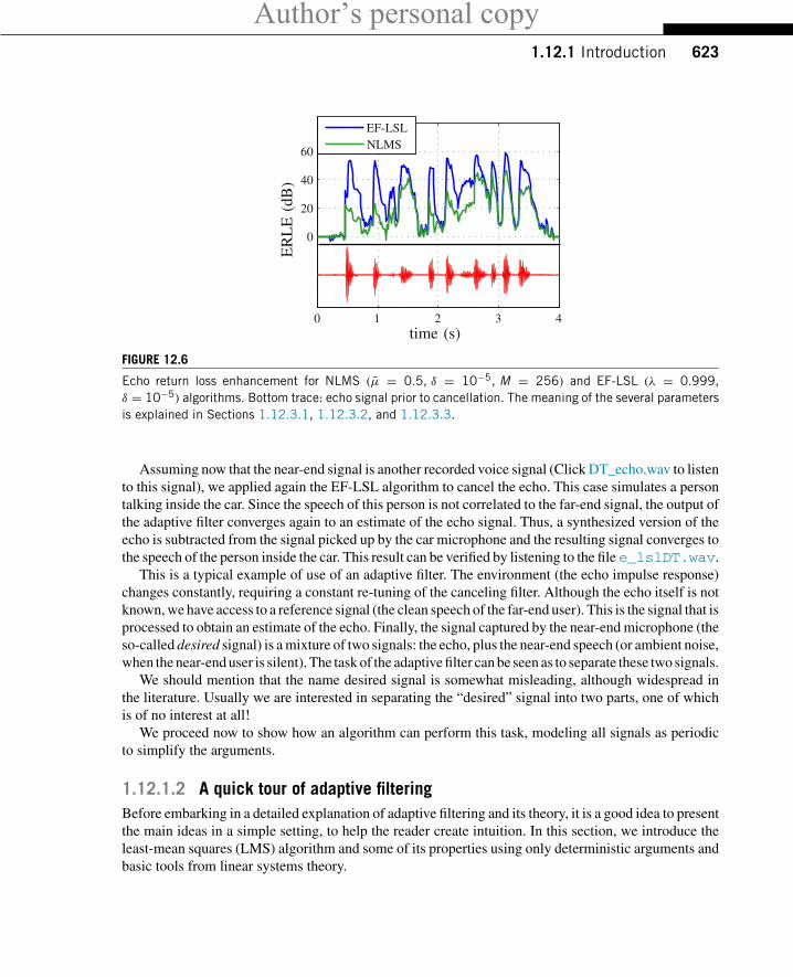
Figure 12.6 shows 4 s of the echo signal, prior to cancellation (bottom) and a measure of the qualityof echo cancellation, the so-called echo return loss enhancement (ERLE) (top). The ERLE is definedas the ratio
ERLE = Power of original echo
Power of residual echo.
The higher the ERLE, the better the performance of the canceler. The ERLE drops when the originalecho is small (there is nothing to cancel!), and increases again when the echo is strong. The figure showsthat EF-LSL performs better than NLMS (but at a higher computational cost).
Author’s personal copy1.12.1 Introduction 623
0
0 1 2 3 4
60
40
20
time (s)
ER
LE
(dB
)
EF-LSLNLMS
FIGURE 12.6
Echo return loss enhancement for NLMS (μ = 0.5, δ = 10−5, M = 256) and EF-LSL (λ = 0.999,δ = 10−5) algorithms. Bottom trace: echo signal prior to cancellation. The meaning of the several parametersis explained in Sections 1.12.3.1, 1.12.3.2, and 1.12.3.3.
Assuming now that the near-end signal is another recorded voice signal (Click DT_echo.wav to listento this signal), we applied again the EF-LSL algorithm to cancel the echo. This case simulates a persontalking inside the car. Since the speech of this person is not correlated to the far-end signal, the output ofthe adaptive filter converges again to an estimate of the echo signal. Thus, a synthesized version of theecho is subtracted from the signal picked up by the car microphone and the resulting signal converges tothe speech of the person inside the car. This result can be verified by listening to the filee_lslDT.wav.
This is a typical example of use of an adaptive filter. The environment (the echo impulse response)changes constantly, requiring a constant re-tuning of the canceling filter. Although the echo itself is notknown, we have access to a reference signal (the clean speech of the far-end user). This is the signal that isprocessed to obtain an estimate of the echo. Finally, the signal captured by the near-end microphone (theso-called desired signal) is a mixture of two signals: the echo, plus the near-end speech (or ambient noise,when the near-end user is silent). The task of the adaptive filter can be seen as to separate these two signals.
We should mention that the name desired signal is somewhat misleading, although widespread inthe literature. Usually we are interested in separating the “desired” signal into two parts, one of whichis of no interest at all!
We proceed now to show how an algorithm can perform this task, modeling all signals as periodicto simplify the arguments.
1.12.1.2 A quick tour of adaptive filteringBefore embarking in a detailed explanation of adaptive filtering and its theory, it is a good idea to presentthe main ideas in a simple setting, to help the reader create intuition. In this section, we introduce theleast-mean squares (LMS) algorithm and some of its properties using only deterministic arguments andbasic tools from linear systems theory.
Author’s personal copy624 CHAPTER 12 Adaptive Filters
x(n)Echo path
y(n)
v(n)
d(n)
+
+
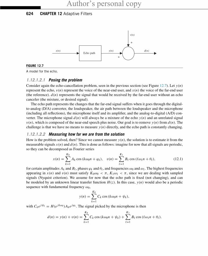
FIGURE 12.7
A model for the echo.
1.12.1.2.1 Posing the problemConsider again the echo-cancellation problem, seen in the previous section (see Figure 12.7). Let y(n)represent the echo, v(n) represent the voice of the near-end user, and x(n) the voice of the far-end user(the reference). d(n) represents the signal that would be received by the far-end user without an echocanceler (the mixture, or desired signal).
The echo path represents the changes that the far-end signal suffers when it goes through the digital-to-analog (D/A) converter, the loudspeaker, the air path between the loudspeaker and the microphone(including all reflections), the microphone itself and its amplifier, and the analog-to-digital (A/D) con-verter. The microphone signal d(n) will always be a mixture of the echo y(n) and an unrelated signalv(n), which is composed of the near-end speech plus noise. Our goal is to remove y(n) from d(n). Thechallenge is that we have no means to measure y(n) directly, and the echo path is constantly changing.
1.12.1.2.2 Measuring how far we are from the solutionHow is the problem solved, then? Since we cannot measure y(n), the solution is to estimate it from themeasurable signals x(n) and d(n). This is done as follows: imagine for now that all signals are periodic,so they can be decomposed as Fourier series
x(n) =K0∑
k=1
Ak cos (kω0n + ϕk), v(n) =K1∑�=1
B� cos (�ω1n + θ�), (12.1)
for certain amplitudes Ak and B�, phases ϕk and θ�, and frequencies ω0 and ω1. The highest frequenciesappearing in x(n) and v(n) must satisfy K0ω0 < π , K1ω1 < π , since we are dealing with sampledsignals (Nyquist criterion). We assume for now that the echo path is fixed (not changing), and canbe modeled by an unknown linear transfer function H(z). In this case, y(n) would also be a periodicsequence with fundamental frequency ω0,
y(n) =K0∑
k=1
Ck cos (kω0n + ψk),
with Cke jψk = H(e jkω0)Ake jϕk . The signal picked by the microphone is then
d(n) = y(n)+ v(n) =K0∑
k=1
Ck cos (kω0n + ψk)+K1∑�=1
B� cos (�ω1n + θ�).
Author’s personal copy1.12.1 Introduction 625
x(n) H(z) y(n)
v(n)
d(n)
y(n)
+
+
+
−H(z)
e(n)
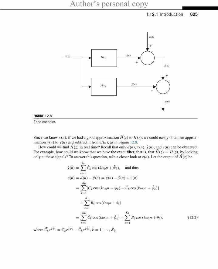
FIGURE 12.8
Echo canceler.
Since we know x(n), if we had a good approximation H(z) to H(z), we could easily obtain an approx-imation y(n) to y(n) and subtract it from d(n), as in Figure 12.8.
How could we find H(z) in real time? Recall that only d(n), x(n), y(n), and e(n) can be observed.For example, how could we know that we have the exact filter, that is, that H(z) = H(z), by lookingonly at these signals? To answer this question, take a closer look at e(n). Let the output of H(z) be
y(n) =k0∑
k=1
Ck cos (kω0n + ψk), and thus
e(n) = d(n)− y(n) = y(n)− y(n)+ v(n)
=K0∑
k=1
[Ck cos (kω0n + ψk)− Ck cos (kω0n + ψk)]
+K1∑�=1
B� cos (�ω1n + θ�)
=K0∑
k=1
Ck cos (kω0n + ψk)+K1∑�=1
B� cos (�ω1n + θ�), (12.2)
where Cke jψk = Cke jψk − Cke jψk , k = 1, . . . , K0.
Author’s personal copy626 CHAPTER 12 Adaptive Filters
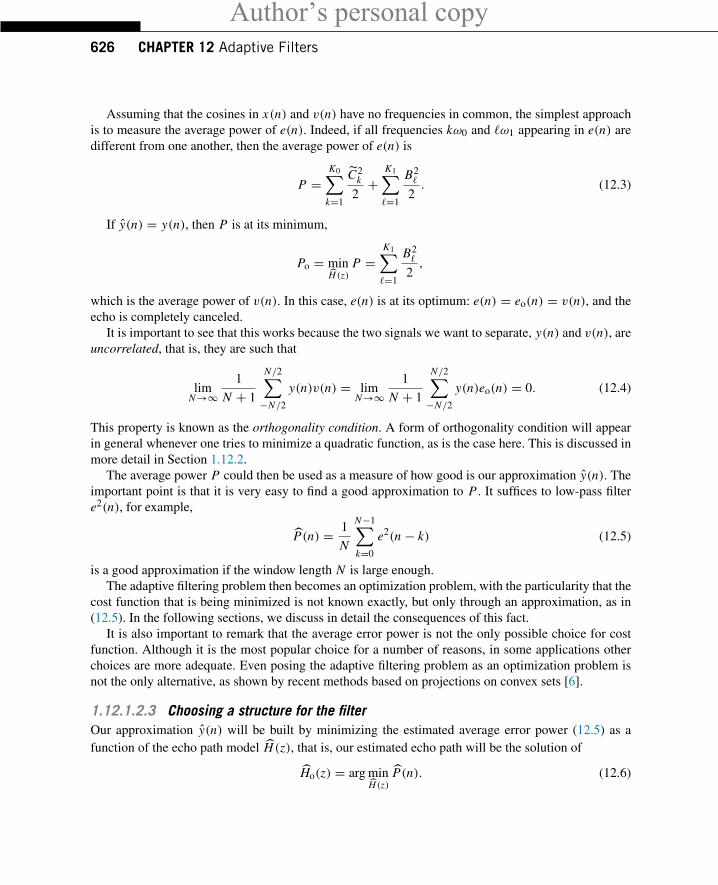
Assuming that the cosines in x(n) and v(n) have no frequencies in common, the simplest approachis to measure the average power of e(n). Indeed, if all frequencies kω0 and �ω1 appearing in e(n) aredifferent from one another, then the average power of e(n) is
P =K0∑
k=1
C2k
2+
K1∑�=1
B2�
2. (12.3)
If y(n) = y(n), then P is at its minimum,
Po = minH(z)
P =K1∑�=1
B2�
2,
which is the average power of v(n). In this case, e(n) is at its optimum: e(n) = eo(n) = v(n), and theecho is completely canceled.
It is important to see that this works because the two signals we want to separate, y(n) and v(n), areuncorrelated, that is, they are such that
limN→∞
1
N + 1
N/2∑−N/2
y(n)v(n) = limN→∞
1
N + 1
N/2∑−N/2
y(n)eo(n) = 0. (12.4)
This property is known as the orthogonality condition. A form of orthogonality condition will appearin general whenever one tries to minimize a quadratic function, as is the case here. This is discussed inmore detail in Section 1.12.2.
The average power P could then be used as a measure of how good is our approximation y(n). Theimportant point is that it is very easy to find a good approximation to P . It suffices to low-pass filtere2(n), for example,
P(n) = 1
N
N−1∑k=0
e2(n − k) (12.5)
is a good approximation if the window length N is large enough.The adaptive filtering problem then becomes an optimization problem, with the particularity that the
cost function that is being minimized is not known exactly, but only through an approximation, as in(12.5). In the following sections, we discuss in detail the consequences of this fact.
It is also important to remark that the average error power is not the only possible choice for costfunction. Although it is the most popular choice for a number of reasons, in some applications otherchoices are more adequate. Even posing the adaptive filtering problem as an optimization problem isnot the only alternative, as shown by recent methods based on projections on convex sets [6].
1.12.1.2.3 Choosing a structure for the filterOur approximation y(n) will be built by minimizing the estimated average error power (12.5) as afunction of the echo path model H(z), that is, our estimated echo path will be the solution of
Ho(z) = arg minH(z)
P(n). (12.6)
Author’s personal copy1.12.1 Introduction 627
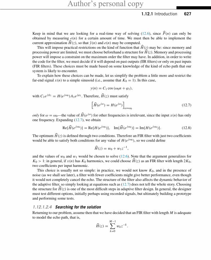
Keep in mind that we are looking for a real-time way of solving (12.6), since P(n) can only beobtained by measuring e(n) for a certain amount of time. We must then be able to implement thecurrent approximation H(z), so that y(n) and e(n) may be computed.
This will impose practical restrictions on the kind of function that H(z) may be: since memory andprocessing power are limited, we must choose beforehand a structure for H(z). Memory and processingpower will impose a constraint on the maximum order the filter may have. In addition, in order to writethe code for the filter, we must decide if it will depend on past outputs (IIR filters) or only on past inputs(FIR filters). These choices must be made based on some knowledge of the kind of echo path that oursystem is likely to encounter.
To explain how these choices can be made, let us simplify the problem a little more and restrict thefar-end signal x(n) to a simple sinusoid (i.e., assume that K0 = 1). In this case,
y(n) = C1 cos (ω0n + ϕ1),
with C1e jψ1 = H(e jω0)A1e jϕ1 . Therefore, H(z) must satisfy[H(e jω) = H(e jω)
]ω=ω0
(12.7)
only for ω = ω0—the value of H(e jω) for other frequencies is irrelevant, since the input x(n) has onlyone frequency. Expanding (12.7), we obtain
Re{H(e jω0)} = Re{H(e jω0)}, Im{H(e jω0)} = Im{H(e jω0)}. (12.8)
The optimum H(z) is defined through two conditions. Therefore an FIR filter with just two coefficientswould be able to satisfy both conditions for any value of H(e jω0), so we could define
H(z) = w0 + w1z−1,
and the values of w0 and w1 would be chosen to solve (12.6). Note that the argument generalizes forK0 > 1: in general, if x(n) has K0 harmonics, we could choose H(z) as an FIR filter with length 2K0,two coefficients per input harmonic.
This choice is usually not so simple: in practice, we would not know K0, and in the presence ofnoise (as we shall see later), a filter with fewer coefficients might give better performance, even thoughit would not completely cancel the echo. The structure of the filter also affects the dynamic behavior ofthe adaptive filter, so simply looking at equations such as (12.7) does not tell the whole story. Choosingthe structure for H(z) is one of the most difficult steps in adaptive filter design. In general, the designermust test different options, initially perhaps using recorded signals, but ultimately building a prototypeand performing some tests.
1.12.1.2.4 Searching for the solutionReturning to our problem, assume then that we have decided that an FIR filter with length M is adequateto model the echo path, that is,
H(z) =M−1∑k=0
wk z−k .
Author’s personal copy628 CHAPTER 12 Adaptive Filters
Our minimization problem (12.6) now reduces to finding the coefficients w0, . . . , wM−1 that solve
minw0,...,wM−1
P(n). (12.9)
Since P(n)must be computed from measurements, we must use an iterative method to solve (12.9).Many algorithms could be used, as long as they depend only on measurable quantities (x(n), d(n), y(n),and e(n)). We will use the steepest descent algorithm (also known as gradient algorithm) as an examplenow. Later we show other methods that also could be used. If you are not familiar with the gradientalgorithm, see Box 1 for an introduction.
The cost function in (12.9) is
P(n) = 1
N
N−1∑k=0
e2(n − k) = 1
N
N−1∑k=0
[d(n − k)− y(n − k)]2.
We need to rewrite this equation so that the steepest descent algorithm can be applied. Recall also thatnow the filter coefficients will change, so define the vectors
w(n) = [w0(n) w1(n) · · · wM−1(n)]T ,and
x(n) = [x(n) x(n − 1) · · · x(n − M + 1)]T ,where (·)T denotes transposition. At each instant, we have y(n) = wT (n)x(n), and our cost functionbecomes
P(n) = 1
N
N−1∑k=0
[d(n − k)− wT (n − k)x(n − k)
]2, (12.10)
which depends on w(n), . . . ,w(n − N + 1). In order to apply the steepest descent algorithm, let uskeep the coefficient vector w(n) constant during the evaluation of P , as follows. Starting from an initialcondition w(0), compute for n = 0, N , 2N , . . . (The notation is explained in Boxes 2 and 6.)
w(n + N ) = w(n)− α ∂ P(n + N − 1)
∂wT
∣∣∣∣w=w(n)
, (12.11)
where α is a positive constant, and w(n + N − 1) = w(n + N − 2) = · · · = w(n). Our cost functionnow depends on only one w(n) (compare with (12.10)):
P(n + N − 1) = 1
N
N−1∑k=0
[d(n + N − 1− k)− wT (n)x(n + N − 1− k)
]2
= 1
N
N−1∑k=0
[d(n + k)− wT (n)x(n + k)
]2, n = 0, N , 2N , . . . (12.12)
We now need to evaluate the gradient of P . Expanding the expression above, we obtain
P(n + N − 1) = 1
N
N−1∑k=0
[d(n + k)−
M−1∑�=0
w�(n)x(n + k − �)]2
,
Author’s personal copy1.12.1 Introduction 629
so
∂ P(n − N + 1)
∂wm(n)= − 2
N
N−1∑k=0
[d(n + k)− wT (n)x(n + k)
]x(n + k − m)
= − 2
N
N−1∑k=0
e(n + k)x(n + k − m),
and∂ P(n − N + 1)
∂wT= − 2
N
N−1∑k=0
e(n + k)x(n + k), n = 0, N , 2N , . . . (12.13)
As we needed, this gradient depends only on measurable quantities, e(n + k) and x(n + k), fork = 0, . . . , N − 1. Our algorithm for updating the filter coefficients then becomes
w(n + N ) = w(n)+ μ 1
N
N−1∑k=0
e(n + k)x(n + k), n = 0, N , 2N , . . . , (12.14)
where we introduced the overall step-size μ = 2α.We still must choose μ and N . The choice of μ is more complicated and will be treated in Sec-
tion 1.12.1.2.5. The value usually employed for N may be a surprise: in almost all cases, one usesN = 1, resulting in the so-called least-mean squares (LMS) algorithm
w(n + 1) = w(n)+ μe(n)x(n), (12.15)
proposed initially by Widrow and Hoff in 1960 [7] (Widrow [8] describes the history of the creationof the LMS algorithm). The question is, how can this work, if no average is being used for estimatingthe error power? An intuitive answer is not complicated: assume that μ is a very small number so thatμ = μ0/N for a large N . In this case, we can approximate e(n + k) from (12.15) as follows.
w(n + 1) = w(n)+ μ0
Ne(n)x(n) ≈ w(n), if N is large.
Since w(n+1) ≈ w(n), we have e(n+1) = d(n+1)−wT (n+1)x(n+1) ≈ d(n+1)−wT (n)x(n+1).Therefore, we could approximate
e(n + k) ≈ d(n + k)− wT (n)x(n + k), k = 0, . . . , N − 1,
so N steps of the LMS recursion (12.15) would result
w(n + N ) ≈ w(n)+ μ0
N
N−1∑k=0
[d(n + k)− wT (n)x(n + k)
]x(n + k),
just what would be obtained from (12.14). The conclusion is that, although there is no explicit averagebeing taken in the LMS algorithm (12.15), the algorithm in fact computes an implicit, approximateaverage if the step-size is small. This is exactly what happens, as can be seen in the animations in
Author’s personal copy630 CHAPTER 12 Adaptive Filters
(a) µ = (b) µ = 0.50.1
(c) µ = 1.1 (d) µ = 1.9
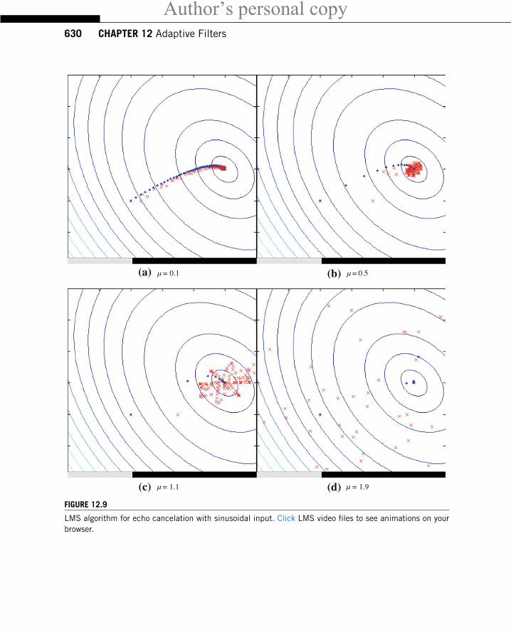
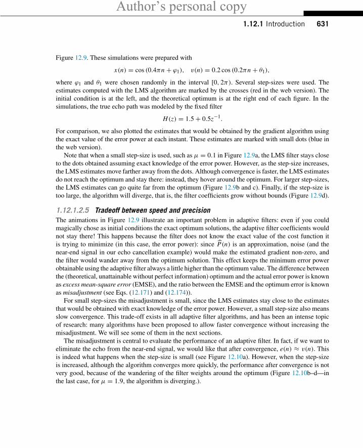
FIGURE 12.9
LMS algorithm for echo cancelation with sinusoidal input. Click LMS video files to see animations on yourbrowser.
Author’s personal copy1.12.1 Introduction 631
Figure 12.9. These simulations were prepared with
x(n) = cos (0.4πn + ϕ1), v(n) = 0.2 cos (0.2πn + θ1),
where ϕ1 and θ1 were chosen randomly in the interval [0, 2π). Several step-sizes were used. Theestimates computed with the LMS algorithm are marked by the crosses (red in the web version). Theinitial condition is at the left, and the theoretical optimum is at the right end of each figure. In thesimulations, the true echo path was modeled by the fixed filter
H(z) = 1.5+ 0.5z−1.
For comparison, we also plotted the estimates that would be obtained by the gradient algorithm usingthe exact value of the error power at each instant. These estimates are marked with small dots (blue inthe web version).
Note that when a small step-size is used, such as μ = 0.1 in Figure 12.9a, the LMS filter stays closeto the dots obtained assuming exact knowledge of the error power. However, as the step-size increases,the LMS estimates move farther away from the dots. Although convergence is faster, the LMS estimatesdo not reach the optimum and stay there: instead, they hover around the optimum. For larger step-sizes,the LMS estimates can go quite far from the optimum (Figure 12.9b and c). Finally, if the step-size istoo large, the algorithm will diverge, that is, the filter coefficients grow without bounds (Figure 12.9d).
1.12.1.2.5 Tradeoff between speed and precisionThe animations in Figure 12.9 illustrate an important problem in adaptive filters: even if you couldmagically chose as initial conditions the exact optimum solutions, the adaptive filter coefficients wouldnot stay there! This happens because the filter does not know the exact value of the cost function itis trying to minimize (in this case, the error power): since P(n) is an approximation, noise (and thenear-end signal in our echo cancellation example) would make the estimated gradient non-zero, andthe filter would wander away from the optimum solution. This effect keeps the minimum error powerobtainable using the adaptive filter always a little higher than the optimum value. The difference betweenthe (theoretical, unattainable without perfect information) optimum and the actual error power is knownas excess mean-square error (EMSE), and the ratio between the EMSE and the optimum error is knownas misadjustment (see Eqs. (12.171) and (12.174)).
For small step-sizes the misadjustment is small, since the LMS estimates stay close to the estimatesthat would be obtained with exact knowledge of the error power. However, a small step-size also meansslow convergence. This trade-off exists in all adaptive filter algorithms, and has been an intense topicof research: many algorithms have been proposed to allow faster convergence without increasing themisadjustment. We will see some of them in the next sections.
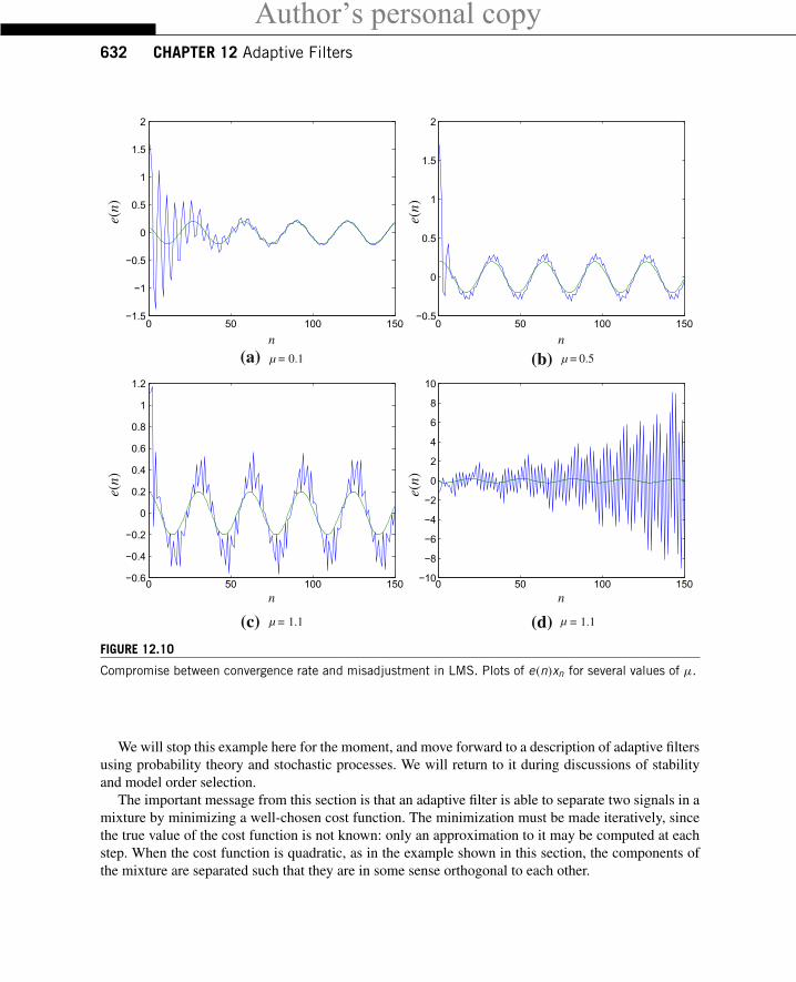
The misadjustment is central to evaluate the performance of an adaptive filter. In fact, if we want toeliminate the echo from the near-end signal, we would like that after convergence, e(n) ≈ v(n). Thisis indeed what happens when the step-size is small (see Figure 12.10a). However, when the step-sizeis increased, although the algorithm converges more quickly, the performance after convergence is notvery good, because of the wandering of the filter weights around the optimum (Figure 12.10b–d—inthe last case, for μ = 1.9, the algorithm is diverging.).
Author’s personal copy632 CHAPTER 12 Adaptive Filters
0 50 100 150−1.5
−1
−0.5
0
0.5
1
1.5
2
n0 50 100 150
−0.5
0
0.5
1
1.5
2
n
0 50 100 150−0.6
−0.4
−0.2
0
0.2
0.4
0.6
0.8
1
1.2
n0 50 100 150−10
−8
−6
−4
−2
0
2
4
6
8
10
n
(a) µ = (b) µ = 0.50.1
(c)
e(n)
e(n)
e(n)
e(n)
µ = 1.1 (d) µ = 1.1
FIGURE 12.10
Compromise between convergence rate and misadjustment in LMS. Plots of e(n)xn for several values of μ.
We will stop this example here for the moment, and move forward to a description of adaptive filtersusing probability theory and stochastic processes. We will return to it during discussions of stabilityand model order selection.
The important message from this section is that an adaptive filter is able to separate two signals in amixture by minimizing a well-chosen cost function. The minimization must be made iteratively, sincethe true value of the cost function is not known: only an approximation to it may be computed at eachstep. When the cost function is quadratic, as in the example shown in this section, the components ofthe mixture are separated such that they are in some sense orthogonal to each other.
Author’s personal copy1.12.1 Introduction 633
Box 1: Steepest descent algorithm
Given a cost functionJ (w) = J (w0, . . . , wM−1),
with w = [w0, . . . , wM−1]T ((·)T denotes transposition), we want to find the minimum of J , that is,we want to find wo such that
wo = arg minw
J (w).
The solution can be found using the gradient of J (w), which is defined by
∇w J (w) = ∂ J
∂wT=
⎡⎢⎢⎢⎢⎣∂ J∂w0∂ J∂w1...∂ J
∂wM−1
⎤⎥⎥⎥⎥⎦ .See Box 2 for a brief explanation about gradients and Hessians, that is, derivatives of functions of severalvariables.The notation ∂ J/∂wT is most convenient when we deal with complex variables, as in Box 6. We use itfor real variables for consistency.
Since the gradient always points to the direction in which J (w) increases most quickly, the steepestdescent algorithm searches iteratively for the minimum of J (w) taking at each iteration a small step inthe opposite direction, i.e., towards −∇w J (w):
w(n + 1) = w(n)− μ2
∇w J (w(n)), (12.16)
where μ is a step-size, i.e., a constant controlling the speed of the algorithm. As we shall see, thisconstant should not be too small (or the algorithm will converge too slowly) neither too large (or therecursion will diverge).
As an example, consider the quadratic cost function with M = 2
J (w) = 1− 2wT r + wT Rw, (12.17)
with
r =[
10
], R =
[43 − 2
3
− 23
43
]. (12.18)
The gradient of J (w) is
∇w J (w) = ∂ J
∂wT= −2r + 2Rw. (12.19)
Of course, for this example we can find the optimum wo by equating the gradient to zero:
∇w J (wo) = 0 =⇒ Rwo = r =⇒ wo = R−1r =[
0.98770.4902
]. (12.20)
Author’s personal copy634 CHAPTER 12 Adaptive Filters
Note that in this case the Hessian of J (w) (the matrix of second derivatives, see Box 2) is simply∇2
w J = 2R. As R is symmetric with positive eigenvalues (λ1 = 2 and λ2 = 23 ), it is positive-definite,
and we can conclude that wo is indeed a minimum of J (w) (See Boxes 2 and 3. Box 3 lists severaluseful properties of matrices.)
Even though in this case we could compute the optimum solution through (12.20), we will apply thegradient algorithm with the intention of understanding how it works and which are its main limitations.From (12.16) and (12.17), we obtain the recursion
w(n + 1) = w(n)+ μ(r − Rw(n)). (12.21)
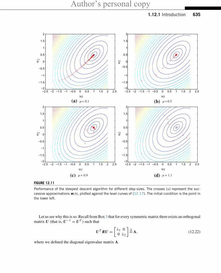
The user must choose an initial condition w(0).In Figure 12.11 we plot the evolution of the approximations computed through (12.21) against the
level sets (i.e., curves of constant value) of the cost function (12.17). Different choices of step-sizeμ areshown. In Figure 12.11a, a small step-size is used. The algorithm converges to the correct solution, butslowly. In Figure 12.11b, we used a larger step-size—convergence is now faster, but the algorithm stillneeds several iterations to reach the solution. If we try to increase the step-size even further, convergenceat first becomes slower again, with the algorithm oscillating towards the solution (Figure 12.11c). Foreven larger step-sizes, such as that in Figure 12.11d, the algorithm diverges: the filter coefficients getfarther and farther away from the solution.
It is important to find the maximum step-size for which the algorithm (12.21) remains stable. Forthis, we need concepts from linear systems and linear algebra, in particular eigenvalues, their relation tostability of linear systems, and the fact that symmetric matrices always have real eigenvalues (see Box 3).
The range of allowed step-sizes is found as follows. Rewrite (12.21) as
w(n + 1) = [I − μR
]w(n)+ μr,
which is a linear recursion in state-space form (I is the identity matrix).Linear systems theory [9] tells us that this recursion converges as long as the largest eigenvalue of
A = I − μR has absolute value less than one. The eigenvalues of A are the roots of
det (β I − (I − μR)) = det ((β − 1)I + μR) = − det ((1− β)I − μR) = 0.
Let 1−β = ν. Then β is an eigenvalue of A if and only if ν = 1−β is an eigenvalue of μR. Therefore,if we denote by λi the eigenvalues of R, the stability condition is
−1 < 1− μλi < 1 ∀i ⇔ 0 < μ <2
λi∀i ⇔ 0 < μ <
2
max{λi } .The stability condition for our example is thus 0 < μ < 1, in agreement with what we saw inFigure 12.11.
The gradient algorithm leads to relatively simple adaptive filtering algorithms; however, it has animportant drawback. As you can see in Figure 12.11a, the gradient does not point directly to the directionof the optimum. This effect is heightened when the level sets of the cost function are very elongated,as in Figure 12.12. This case corresponds to a quadratic function in which R has one eigenvalue muchsmaller than the other. In this example, we replaced the matrix R in (12.18) by
R′ = 1
9
[25 2020 25
].
This matrix has eigenvalues λ′1 = 5 and λ′2 = 59 .
Author’s personal copy1.12.1 Introduction 635
−2.5 −2 −1.5 −1 −0.5 0 0.5 1 1.5 2 2.5−2
−1.5
−1
−0.5
0
0.5
1
1.5
2
w1
w2
−2.5 −2 −1.5 −1 −0.5 0 0.5 1 1.5 2 2.5−2
−1.5
−1
−0.5
0
0.5
1
1.5
2
w1
w 2
−2.5 −2 −1.5 −1 −0.5 0 0.5 1 1.5 2 2.5−2
−1.5
−1
−0.5
0
0.5
1
1.5
2
w1
w 2
−2.5 −2 −1.5 −1 −0.5 0 0.5 1 1.5 2 2.5−2
−1.5
−1
−0.5
0
0.5
1
1.5
2
w1
w 2
(a) µ = (b) µ = 0.50.1
(c) µ = 0.9 (d) µ = 1.1
FIGURE 12.11
Performance of the steepest descent algorithm for different step-sizes. The crosses (x) represent the suc-cessive approximations w(n), plotted against the level curves of (12.17). The initial condition is the point inthe lower left.
Let us see why this is so. Recall from Box 3 that for every symmetric matrix there exists an orthogonalmatrix U (that is, U−1 = U T ) such that
U T RU =[λ1 00 λ2
]�=�, (12.22)
where we defined the diagonal eigenvalue matrix �.
Author’s personal copy636 CHAPTER 12 Adaptive Filters
Let us apply a change of coordinates to (12.19). The optimum solution to (12.17) is
wo = R−1r.
Our first change of coordinates is to replace w(n) by w(n) = wo − w(n) in (12.19). Subtract (12.19)from wo and replace r in (12.19) by r = Rwo to obtain
w(n + 1) = w(n)− μRw(n) = [I − μR
]w(n). (12.23)
Next, multiply this recursion from both sides by UT = U−1
U T w(n + 1) = UT [I − μR
]UUT︸ ︷︷ ︸=I
w(n) = [I − μ�
]UT w(n).
Defining w(n) = UT w(n), we have rewritten the gradient equation in a new set of coordinates, suchthat now the equations are uncoupled. Given that � is diagonal, the recursion is simply[
w1(n + 1)w2(n + 1)
]=[(1− μλ1)w1(n)(1− μλ2)w2(n)
]. (12.24)
Note that, as long as |1 − μλi | < 1 for i = 1, 2, both entries of w(n) will converge to zero, andconsequently w(n) will converge to wo.
The stability condition for this recursion is
|1− μλi | < 1, i = 1, 2⇒ μ <2
max{λ1, λ2} .
−2.5 −2 −1.5 −1 −0.5 0 0.5 1 1.5 2 2.5−2
−1.5
−1
−0.5
0
0.5
1
1.5
2
w1
w2
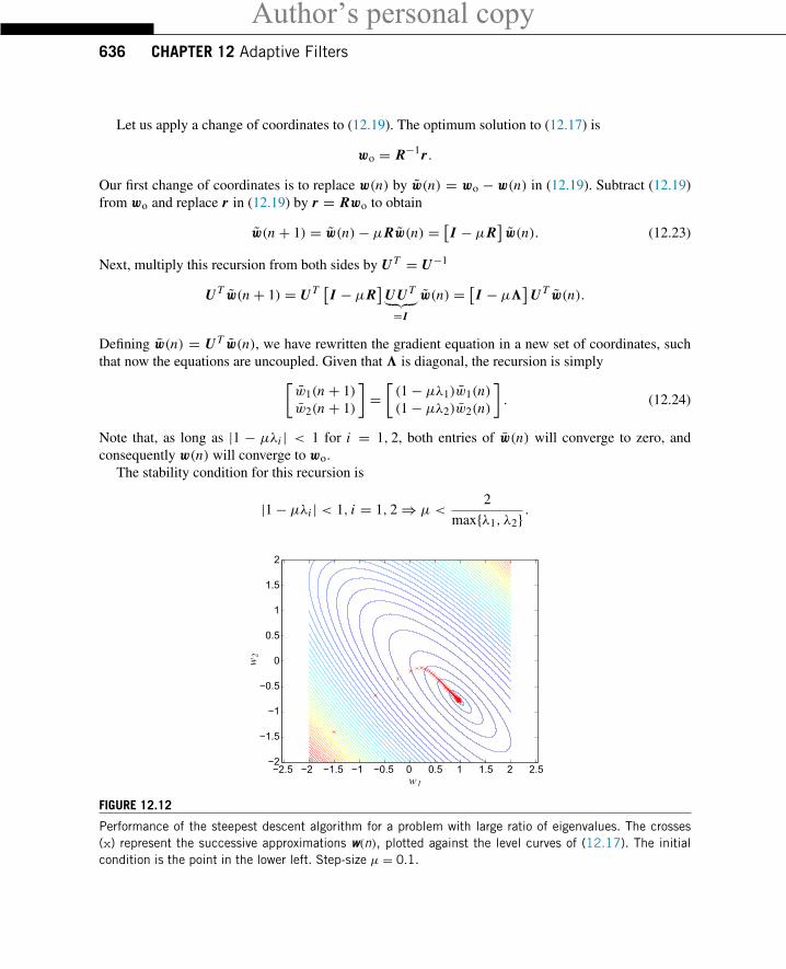
FIGURE 12.12
Performance of the steepest descent algorithm for a problem with large ratio of eigenvalues. The crosses(x) represent the successive approximations w(n), plotted against the level curves of (12.17). The initialcondition is the point in the lower left. Step-size μ = 0.1.
Author’s personal copy1.12.1 Introduction 637
When one of the eigenvalues is much larger than the other, say, when λ1 λ2, the rate of convergencefor the direction relative to the smaller eigenvalue becomes
1 > 1− μλ2 > 1− 2λmin
λmax≈ 1,
and even if one of the coordinates in w(n) converges quickly to zero, the other will converge very slowly.This is what we saw in Figure 12.12. The ratio λmax/λmin is known as the eigenvalue spread of a matrix.
In general, the gradient algorithm converges slowly when the eigenvalue spread of the Hessian islarge. One way of solving this problem is to use a different optimization algorithm, such as the Newtonor quasi-Newton algorithms, which use the inverse of the Hessian matrix, or an approximation to it, toimprove the search direction used by the gradient algorithm.
Although these algorithms converge very quickly, they require more computational power, comparedto the gradient algorithm. We will see more about them when we describe the RLS (recursive least-squares) algorithm in Section 1.12.3.3.
For example, for the quadratic cost-function (12.17), the Hessian is equal to 2R. If we had a goodapproximation R to R, we could use the recursion
w(n + 1) = w(n)+ μR−1[r − Rw(n)]. (12.25)
This class of algorithms is known as quasi-Newton (if R−1
is an approximation) or Newton (if R−1
isexact). In the Newton case, we would have
w(n + 1) = (1− μ)w(n)+ wo,
that is, the algorithm moves at each step precisely in the direction of the optimum solution. Of course,this is not a very interesting algorithm for a quadratic cost function as in this example (the optimumsolution is used in the recursion!) However, this method is very useful when the cost function is notquadratic and in adaptive filtering, when the cost function is not known exactly.
Box 2: Gradients
Consider a function of several variables J (w), where
w =
⎡⎢⎢⎢⎣w0w1...
wM−1
⎤⎥⎥⎥⎦ .Its gradient is defined by
∇w J (w) = ∂ J
∂wT=
⎡⎢⎢⎢⎢⎣∂ J∂w0∂ J∂w1...∂ J
∂wM−1
⎤⎥⎥⎥⎥⎦ .
Author’s personal copy638 CHAPTER 12 Adaptive Filters
The real value of the notation ∂ J/∂wT will only become apparent when working with functions ofcomplex variables, as shown in Box 6. We also define, for consistency,
∂ J
∂w=[∂ J∂w0
∂ J∂w1
. . . ∂ J∂wM−1
].
As an example, consider the quadratic cost function
J (w) = b − 2wT r + wT Rw. (12.26)
The gradient of J (w) is (verify!)
∇w J (w) = ∂ J
∂wT= −2r + 2Rw. (12.27)
If we use the gradient to find the minimum of J (w), it would be necessary also to check the second-order derivative, to make sure the solution is not a maximum or a saddle point. The second orderderivative of a function of several variables is a matrix, the Hessian. It is defined by
∇2w J = ∂2 J
∂w ∂wT=
⎡⎢⎢⎢⎣∂∂w
{∂ J∂w0
}...
∂∂w
{∂ J
∂wM−1
}⎤⎥⎥⎥⎦ =
⎡⎢⎢⎢⎣∂2 J∂w2
0. . . ∂2 J
∂w0 ∂wM−1
.... . .
...∂2 J
∂wM−1 ∂w0. . . ∂2 J
∂w2M−1
⎤⎥⎥⎥⎦ . (12.28)
Note that for the quadratic cost-function (12.26), the Hessian is equal to R + RT . It is equal to 2R ifR is symmetric, that is, if RT = R. This will usually be the case here. Note that R + RT is alwayssymmetric: in fact, since for well-behaved functions J it holds that
∂2 J
∂wi ∂w j= ∂2 J
∂w j ∂wi,
the Hessian is usually symmetric.Assume that we want to find the minimum of J (w). The first-order conditions are then
∂ J
∂w
∣∣∣∣wo
= 0.
The solution wo is a minimum of J (w) if the Hessian at wo is a positive semi-definite matrix, that is, if
xT ∇2w J (wo)x ≥ 0
for all directions x.
Author’s personal copy1.12.1 Introduction 639
Box 3: Useful results from Matrix Analysis
Here we list without proof a few useful results from matrix analysis. Detailed explanations can be found,for example, in [10–13].
Fact 1 (Traces). The trace of a matrix A ∈ CM×M is the sum of its diagonal elements:
Tr(A) =M∑
i=1
aii , (12.29)
in which the aii are the entries of A. For any two matrices B ∈ CM×N and C ∈ CN×M , it holds that
Tr(BC) = Tr(C B). (12.30)
In addition, if λi , i = 1, . . . ,M are the eigenvalues of a square matrix A ∈ CM×M , then
Tr(A) =M∑
i=1
λi . (12.31)
Fact 2 (Singular matrices). A matrix A ∈ CM×M is singular if and only if there exists a nonzerovector u such that Au = 0.
The null space, or kernel N (A) of a matrix A ∈ CM×N is the set of vectors u ∈ CN such that Au = 0.A square matrix A ∈ CM×M is nonsingular if, and only if, N (A) = {0}, that is, if its null space containsonly the null vector.
Note that, if A = ∑Kk=1 ukv
Hk , with uk, vk ∈ CM , then A cannot be invertible if K < M . This is
because when K < M , there always exists a nonzero vector x ∈ CM such that vHk x = 0 for 1 ≤ k ≤ K ,
and thus Ax = 0 with x = 0.
Fact 3 (Inverses of block matrices). Assume the square matrix A is partitioned such that
A =[
A11 A12A21 A22
],
with A11 and A22 square. If A and A11 are invertible (nonsingular), then
A−1 =[
I −A−111 A12
0 I
] [A−1
11 00 �−1
] [I 0
−A21 A−111 I
],
where � = A22 − A21 A−111 A12 is the Schur complement of A11 in A. If A22 and A are invertible, then
A−1 =[
I 0−A−1
22 A21 I
] [�′−1 00 A−1
22
] [I −A12 A−1
220 I
],
where �′ = A11 − A12 A−122 A21.
Author’s personal copy640 CHAPTER 12 Adaptive Filters
Fact 4 (Matrix inversion Lemma). Let A and B be two nonsingular M × M matrices, D ∈ CK×K
be also nonsingular, and C, E ∈ CM×K be such that
A = B + C DE H . (12.32)
The inverse of A is then given by
A−1 = B−1 − B−1C(D−1 + E H B−1C)−1 E H B−1. (12.33)
The lemma is most useful when K � M . In particular when K = 1, D + E H B−1C is a scalar, andwe have
A−1 = B−1 − B−1C E H B−1
D−1 + E H B−1C.
Fact 5 (Symmetric matrices). Let A ∈ CM×M be Hermitian Symmetric (or simply Hermitian), that
is, AH = (AT )∗ = A. Then, it holds that
1. All eigenvalues λi , i = 1, . . . ,M of A are real.2. A has a complete set of orthonormal eigenvectors ui , i = 1, . . . ,M . Since the eigenvectors are
orthonormal, uHi u j = δi j , where δi j = 1 if i = j and 0 otherwise.
3. Arranging the eigenvectors in a matrix U = [u1 . . . uM
], we find that U is unitary, that is, U H U =
UU H = I . In addition,
U H AU = � =
⎡⎢⎢⎢⎣λ1 0 . . . 00 λ2 . . . 0....... . .
...
0 0 . . . λM
⎤⎥⎥⎥⎦ .4. If A = AT ∈ RM×M , it is called simply symmetric. In this case, not only the eigenvalues, but also
the eigenvectors are real.5. If A is symmetric and invertible, then A−1 is also symmetric.
Fact 6 (Positive-definite matrices). If A ∈ CM×M is Hermitian symmetric and moreover for allu ∈ CM it holds that
uH Au ≥ 0, (12.34)
then A is positive semi-definite. Positive semi-definite matrices have non-negative eigenvalues: λi ≥ 0,i = 1, . . . ,M . They may be singular, if one or more eigenvalue is zero.
If the inequality (12.34) is strict, that is, if
uH Au > 0 (12.35)
for all u = 0, then A is positive-definite. All eigenvalues λi of positive-definite matrices satisfy λi > 0.Positive-definite matrices are always nonsingular.
Finally, all positive-definite matrices admit a Cholesky factorization, i.e., if A is positive-definite,there is a lower-triangular matrix L such that A = LL H [14].
Author’s personal copy1.12.1 Introduction 641
Fact 7 (Norms and spectral radius). The spectral radius ρ(A) of a matrix A ∈ CM×M is
ρ(A) = max1≤i≤M
|λi |, (12.36)
in which λi are the eigenvalues of A. The spectral radius is important, because a linear system
x(n + 1) = Ax(n)
is stable if and only if ρ(A) ≤ 1, as is well known. A useful inequality is that, for any matrix norm ‖ · ‖such that for any A, B ∈ CM×M
‖AB‖ ≤ ‖A‖‖B‖,it holds that
ρ(A) ≤ ‖A‖. (12.37)
This property is most useful when used with norms that are easy to evaluate, such as the 1-norm,
‖A‖1 = max1≤i≤M
M∑j=1
|ai j |,
where ai j are the entries of A. We could also use the infinity norm,
‖A‖∞ = max1≤ j≤M
M∑i=1
|ai j |.
1.12.1.3 ApplicationsDue to the ability to adjust themselves to different environments, adaptive filters can be used in differentsignal processing and control applications. Thus, they have been used as a powerful device in severalfields, such as communications, radar, sonar, biomedical engineering, active noise control, modeling,etc. It is common to divide these applications into four groups:
1. interference cancellation;2. system identification;3. prediction; and4. inverse system identification.
In the first three cases, the goal of the adaptive filter is to find an approximation y(n) for the signaly(n), which is contained in the signal d(n) = y(n) + v(n). Thus, as y(n) approaches y(n), the signale(n) = d(n) − y(n) approaches v(n). The difference between these applications is in what we areinterested. In interference cancellation, we are interested in the signal v(n), as is the case of acousticecho cancellation, where v(n) is the speech of the person using the hands-free telephone (go backto Figures 12.4 and 12.7). In system identification, we are interested in the filter parameters, and in
Author’s personal copy642 CHAPTER 12 Adaptive Filters
adaptivefilter
d(n) v(n)
y(n)e(n)
x(n)
ˆ(n)y
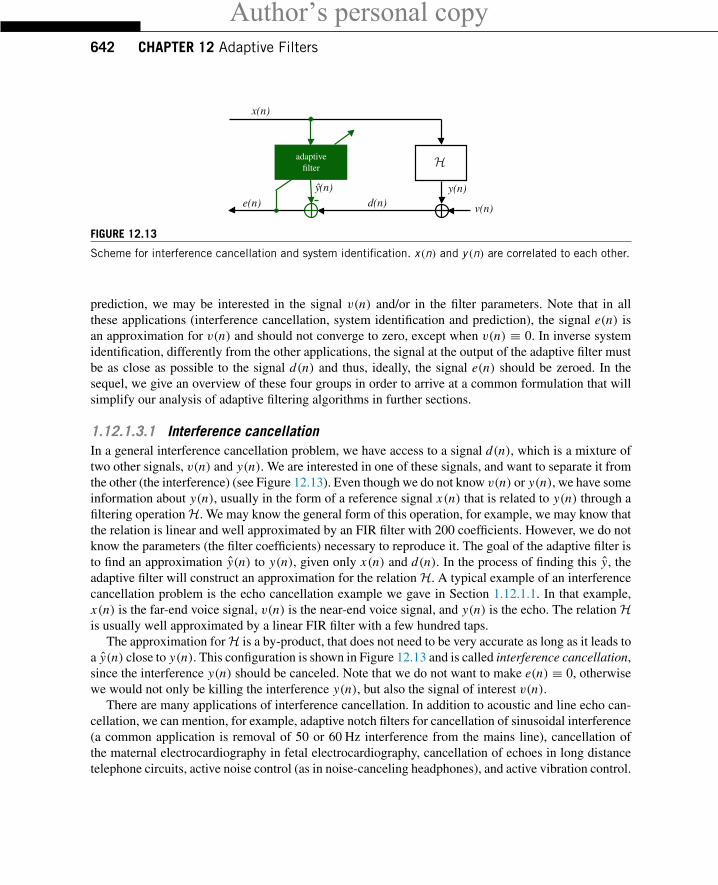
FIGURE 12.13
Scheme for interference cancellation and system identification. x(n) and y (n) are correlated to each other.
prediction, we may be interested in the signal v(n) and/or in the filter parameters. Note that in allthese applications (interference cancellation, system identification and prediction), the signal e(n) isan approximation for v(n) and should not converge to zero, except when v(n) ≡ 0. In inverse systemidentification, differently from the other applications, the signal at the output of the adaptive filter mustbe as close as possible to the signal d(n) and thus, ideally, the signal e(n) should be zeroed. In thesequel, we give an overview of these four groups in order to arrive at a common formulation that willsimplify our analysis of adaptive filtering algorithms in further sections.
1.12.1.3.1 Interference cancellationIn a general interference cancellation problem, we have access to a signal d(n), which is a mixture oftwo other signals, v(n) and y(n). We are interested in one of these signals, and want to separate it fromthe other (the interference) (see Figure 12.13). Even though we do not know v(n) or y(n), we have someinformation about y(n), usually in the form of a reference signal x(n) that is related to y(n) through afiltering operation H. We may know the general form of this operation, for example, we may know thatthe relation is linear and well approximated by an FIR filter with 200 coefficients. However, we do notknow the parameters (the filter coefficients) necessary to reproduce it. The goal of the adaptive filter isto find an approximation y(n) to y(n), given only x(n) and d(n). In the process of finding this y, theadaptive filter will construct an approximation for the relation H. A typical example of an interferencecancellation problem is the echo cancellation example we gave in Section 1.12.1.1. In that example,x(n) is the far-end voice signal, v(n) is the near-end voice signal, and y(n) is the echo. The relation His usually well approximated by a linear FIR filter with a few hundred taps.
The approximation for H is a by-product, that does not need to be very accurate as long as it leads toa y(n) close to y(n). This configuration is shown in Figure 12.13 and is called interference cancellation,since the interference y(n) should be canceled. Note that we do not want to make e(n) ≡ 0, otherwisewe would not only be killing the interference y(n), but also the signal of interest v(n).
There are many applications of interference cancellation. In addition to acoustic and line echo can-cellation, we can mention, for example, adaptive notch filters for cancellation of sinusoidal interference(a common application is removal of 50 or 60 Hz interference from the mains line), cancellation ofthe maternal electrocardiography in fetal electrocardiography, cancellation of echoes in long distancetelephone circuits, active noise control (as in noise-canceling headphones), and active vibration control.
Author’s personal copy1.12.1 Introduction 643
adaptive
filter
d(n)
v(n)
y(n)
e(n)
x(n)
y(n)
controller
controller
controller
plant
parameters
model parametersdesign
reference
specifications
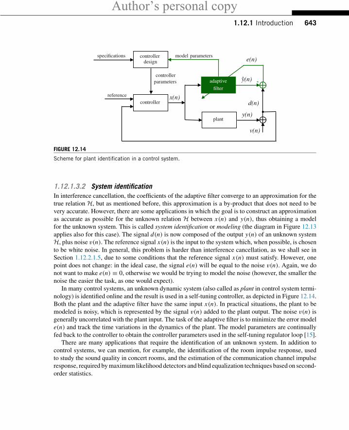
FIGURE 12.14
Scheme for plant identification in a control system.
1.12.1.3.2 System identificationIn interference cancellation, the coefficients of the adaptive filter converge to an approximation for thetrue relation H, but as mentioned before, this approximation is a by-product that does not need to bevery accurate. However, there are some applications in which the goal is to construct an approximationas accurate as possible for the unknown relation H between x(n) and y(n), thus obtaining a modelfor the unknown system. This is called system identification or modeling (the diagram in Figure 12.13applies also for this case). The signal d(n) is now composed of the output y(n) of an unknown systemH, plus noise v(n). The reference signal x(n) is the input to the system which, when possible, is chosento be white noise. In general, this problem is harder than interference cancellation, as we shall see inSection 1.12.2.1.5, due to some conditions that the reference signal x(n) must satisfy. However, onepoint does not change: in the ideal case, the signal e(n) will be equal to the noise v(n). Again, we donot want to make e(n) ≡ 0, otherwise we would be trying to model the noise (however, the smaller thenoise the easier the task, as one would expect).
In many control systems, an unknown dynamic system (also called as plant in control system termi-nology) is identified online and the result is used in a self-tuning controller, as depicted in Figure 12.14.Both the plant and the adaptive filter have the same input x(n). In practical situations, the plant to bemodeled is noisy, which is represented by the signal v(n) added to the plant output. The noise v(n) isgenerally uncorrelated with the plant input. The task of the adaptive filter is to minimize the error modele(n) and track the time variations in the dynamics of the plant. The model parameters are continuallyfed back to the controller to obtain the controller parameters used in the self-tuning regulator loop [15].
There are many applications that require the identification of an unknown system. In addition tocontrol systems, we can mention, for example, the identification of the room impulse response, usedto study the sound quality in concert rooms, and the estimation of the communication channel impulseresponse, required by maximum likelihood detectors and blind equalization techniques based on second-order statistics.
Author’s personal copy644 CHAPTER 12 Adaptive Filters
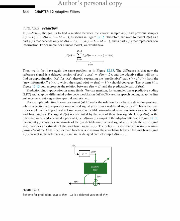
1.12.1.3.3 PredictionIn prediction, the goal is to find a relation between the current sample d(n) and previous samplesd(n − L), . . . , d(n − L − M + 1), as shown in Figure 12.15. Therefore, we want to model d(n) as apart y(n) that depends only on d(n − L), . . . , d(n − L − M + 1), and a part v(n) that represents newinformation. For example, for a linear model, we would have
d(n) =M−1∑k=0
hkd(n − L − k)︸ ︷︷ ︸y(n)
+v(n),
Thus, we in fact have again the same problem as in Figure 12.13. The difference is that now thereference signal is a delayed version of d(n) : x(n) = d(n − L), and the adaptive filter will try tofind an approximation y(n) for y(n), thereby separating the “predictable” part y(n) of d(n) from the“new information” v(n), to which the signal e(n) = d(n) − y(n) should converge. The system H inFigure 12.13 now represents the relation between d(n − L) and the predictable part of d(n).
Prediction finds application in many fields. We can mention, for example, linear predictive coding(LPC) and adaptive differential pulse code modulation (ADPCM) used in speech coding, adaptive lineenhancement, autoregressive spectral analysis, etc.
For example, adaptive line enhancement (ALE) seeks the solution for a classical detection problem,whose objective is to separate a narrowband signal y(n) from a wideband signal v(n). This is the case,for example, of finding a low-level sine wave (predictable narrowband signal) in noise (non-predictablewideband signal). The signal d(n) is constituted by the sum of these two signals. Using d(n) as thereference signal and a delayed replica of it, i.e., d(n−L), as input of the adaptive filter as in Figure 12.15,the output y(n) provides an estimate of the (predictable) narrowband signal y(n), while the error signale(n) provides an estimate of the wideband signal v(n). The delay L is also known as decorrelationparameter of the ALE, since its main function is to remove the correlation between the wideband signalv(n) present in the reference d(n) and in the delayed predictor input d(n − L).
adaptivefilter
d(n)
z − L
e(n)
x(n)
y(n)
FIGURE 12.15
Scheme for prediction. x(n) = d(n − L) is a delayed version of d(n).
Author’s personal copy1.12.1 Introduction 645
adaptivefilter
channel
d(n)z − L
η(n)
e(n)
s(n) x(n) y(n)H(z)
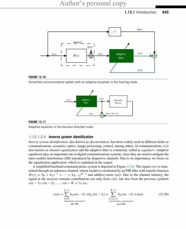
FIGURE 12.16
Simplified communications system with an adaptive equalizer in the training mode.
adaptivefilter
decisiondevice
d(n)=s(n−L)e(n)
x(n) y(n)
ˆ
FIGURE 12.17
Adaptive equalizer in the decision-directed mode.
1.12.1.3.4 Inverse system identificationInverse system identification, also known as deconvolution, has been widely used in different fields ascommunications, acoustics, optics, image processing, control, among others. In communications, it isalso known as channel equalization and the adaptive filter is commonly called as equalizer. Adaptiveequalizers play an important role in digital communications systems, since they are used to mitigate theinter-symbol interference (ISI) introduced by dispersive channels. Due to its importance, we focus onthe equalization application, which is explained in the sequel.
A simplified baseband communications system is depicted in Figure 12.16. The signal s(n) is trans-mitted through an unknown channel, whose model is constituted by an FIR filter with transfer functionH(z) = h0 + h1z−1 + · · · + hK−1zK−1 and additive noise η(n). Due to the channel memory, thesignal at the receiver contains contributions not only from s(n), but also from the previous symbolss(n − 1), s(n − 2), . . . , s(n − K + 1), i.e.,
x(n) =L−1∑k=0
hks(n − k)︸ ︷︷ ︸pre-ISI
+hLs(n − L)+K−1∑
k=L+1
hks(n − k)︸ ︷︷ ︸post-ISI
+η(n). (12.38)
Author’s personal copy646 CHAPTER 12 Adaptive Filters
adaptive
filter
d(n)
e(n)
x(n) y(n)
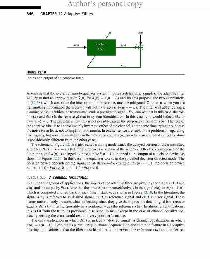
FIGURE 12.18
Inputs and output of an adaptive filter.
Assuming that the overall channel-equalizer system imposes a delay of L samples, the adaptive filterwill try to find an approximation y(n) for d(n) = s(n − L) and for this purpose, the two summationsin (12.38), which constitute the inter-symbol interference, must be mitigated. Of course, when you aretransmitting information the receiver will not have access to d(n − L). The filter will adapt during atraining phase, in which the transmitter sends a pre-agreed signal. You can see that in this case, the roleof x(n) and d(n) is the reverse of that in system identification. In this case, you would indeed like tohave e(n) ≡ 0. The problem is that this is not possible, given the presence of noise in x(n). The role ofthe adaptive filter is to approximately invert the effect of the channel, at the same time trying to suppressthe noise (or at least, not to amplify it too much). In one sense, we are back to the problem of separatingtwo signals, but now the mixture is in the reference signal x(n), so what can and what cannot be doneis considerably different from the other cases.
The scheme of Figure 12.16 is also called training mode, since the delayed version of the transmittedsequence d(n) = s(n − L) (training sequence) is known at the receiver. After the convergence of thefilter, the signal d(n) is changed to the estimate s(n− L) obtained at the output of a decision device, asshown in Figure 12.17. In this case, the equalizer works in the so-called decision-directed mode. Thedecision device depends on the signal constellation—for example, if s(n) = ±1, the decision devicereturns +1 for y(n) ≥ 0, and −1 for y(n) < 0.
1.12.1.3.5 A common formulationIn all the four groups of applications, the inputs of the adaptive filter are given by the signals x(n) andd(n) and the output by y(n). Note that the input d(n) appears effectively in the signal e(n) = d(n)− y(n),which is computed and fed back at each time instant n, as shown in Figure 12.18. In the literature, thesignal d(n) is referred to as desired signal, x(n) as reference signal and e(n) as error signal. Thesenames unfortunately are somewhat misleading, since they give the impression that our goal is to recoverexactly d(n) by filtering (possibly in a nonlinear way) the reference x(n). In almost all applications,this is far from the truth, as previously discussed. In fact, except in the case of channel equalization,exactly zeroing the error would result in very poor performance.
The only application in which d(n) is indeed a “desired signal” is channel equalization, in whichd(n) = s(n− L). Despite this particularity in channel equalization, the common feature in all adaptivefiltering applications is that the filter must learn a relation between the reference x(n) and the desired
Author’s personal copy1.12.2 Optimum Filtering 647
signal d(n) (we will use this name to be consistent with the literature.) In the process of building thisrelation, the adaptive filter is able to perform useful tasks, such as separating two mixed signals; orrecovering a distorted signal. Section 1.12.2 explains this idea in more detail.
1.12.2 Optimum filteringWe now need to extend the ideas of Section 1.12.1.2, that applied only to periodic (deterministic) signals,to more general classes of signals. For this, we will use tools from the theory of stochastic processes.The main ideas are very similar: as before, we need to choose a structure for our filter and a meansof measuring how far or how near we are to the solution. This is done by choosing a convenient costfunction, whose minimum we must search iteratively, based only on measurable signals.
In the case of periodic signals, we saw that minimizing the error power (12.3), repeated below,
P =K0∑
k=1
C2k
2+
K1∑�=1
B2�
2,
would be equivalent to zeroing the echo. However, we were not able to compute the error powerexactly—we used an approximation through a time-average, as in (12.5), repeated here:
P(n) = 1
N
N−1∑k=0
e2(n − k),
where N is a convenient window length (in Section 1.12.1.2, we saw that choosing a large window lengthis approximately equivalent to choosing N = 1 and a small step-size). Since we used an approximatedestimate of the cost, our solution was also an approximation: the estimated coefficients did not convergeexactly to their optimum values, but instead hovered around the optimum (Figures 12.9 and 12.10).
The minimization of the time-average P(n) also works in the more general case in which the echo ismodeled as a random signal—but what is the corresponding exact cost function? The answer is givenby the property of ergodicity that some random signals possess. If a random signal s(n) is such that itsmean E{s(n)} does not depend on n and its autocorrelation E{s(n)s(k)} depends only on n − k, it iscalled wide-sense stationary (WSS) [16]. If s(n) is also (mean-square) ergodic, then
Average power of s(n) = limN→∞
1
N + 1
N∑n=0
s2(n) = E{s2(n)}. (12.39)
Note that E{s2(n)} is an ensemble average, that is, the expected value is computed over all possiblerealizations of the random signal. Relation (12.39) means that for an ergodic signal, the time averageof a single realization of the process is equal to the ensemble-average of all possible realizations of theprocess. This ensemble average is the exact cost function that we would like to minimize.
In the case of adaptive filters, (12.39) holds approximately for e(n) for a finite value of N if theenvironment does not change too fast, and if the filter adapts slowly. Therefore, for random variables wewill still use the average error power as a measure of how well the adaptive filter is doing. The difference
Author’s personal copy648 CHAPTER 12 Adaptive Filters
is that in the case of periodic signals, we could understand the effect of minimizing the average errorpower in terms of the amplitudes of each harmonic in the signal, but now the interpretation will be interms of ensemble averages (variances).
Although the error power is not the only possible choice for cost function, it is useful to study thischoice in detail. Quadratic cost functions such as the error power have a number of properties thatmake them popular. For example, they are differentiable, and so it is relatively easy to find a closed-form solution for the optimum, and in the important case where all signals are Gaussian, the optimumfilters are linear. Of course, quadratic cost functions are not the best option in all situations: the useof other cost functions, or even of adaptive filters not based on the minimization of a cost function, isbecoming more common. We will talk about some of the most important alternatives in Sections 1.12.5.2and 1.12.5.4.
Given the importance of quadratic cost functions, in this section we study them in detail. Our focusis on what could and what could not be done if the filter were able to measure perfectly E{e2(n)} at eachinstant. This discussion has two main goals: the first is to learn what is feasible, so we do not expect morefrom a filter than it can deliver. The second is to enable us to make more knowledgeable choices whendesigning a filter—for example, which filter order should be used, and for system identification, whichinput signal would result in better performance. In Section 1.12.4.4.3 we will study the performance ofadaptive filters taking into consideration their imperfect knowledge of the environment.
1.12.2.1 Linear least-mean squares estimationIn the examples we gave in previous sections, a generic adaptive filtering problem resumed to this: weare given two sequences, {x(n)} and {d(n)}, as depicted in Figure 12.18. It is known, from physicalarguments, that d(n) has two parts, one that is in some sense related to x(n), x(n− 1), . . ., and anotherthat is not, and that both parts are combined additively, that is,
d(n) = H(x(n), x(n − 1), . . . )︸ ︷︷ ︸y(n)
+v(n), (12.40)
where H(·) is an unknown relation, and v(n) is the part “unrelated” to {x(n)}. In our examples so far,H(·)was linear, but we do not need to restrict ourselves to this case. Our objective is to extract y(n) andv(n) from d(n), based only on observations of {x(n)} and {d(n)}. We saw in Section 1.12.1.2 that theaverage power of the difference e(n) between d(n) and our current approximation y(n) could be usedas a measure of how close we are to the solution. In general, H(·) is time-variant, i.e., depends directlyon n. We will not write this dependence explicitly to simplify the notation.
In this section we ask in some sense the inverse problem, that is: given two sequences {x(n)} and{d(n)}, what sort of relation will be found between them if we use E{e2(n)} as a standard? The differenceis that we now do not assume a model such as (12.40); instead, we want to know what kind of modelresults from the exact minimization of E{e2(n)}, where e(n) is defined as the difference between d(n)and a function of x(n), x(n − 1), . . .
We can answer this question in an entirely general way, without specifying beforehand the form ofH. This is done in Box 4. However, if we have information about the physics of a problem and know that
Author’s personal copy1.12.2 Optimum Filtering 649
the relation H(x(n), x(n − 1), . . . ) is of a certain kind, we can restrict the search for the solution H tothis class. This usually reduces the complexity of the filter and increases its convergence rate (becauseless data is necessary to estimate a model with less unknowns, as we will see in Section 1.12.3). In thissection we focus on this second option.
The first task is to describe the class F of allowed functions H. This may be done by choosinga relation that depends on a few parameters, such as (recall that the adaptive filter output is y(n) =H(x(n), x(n − 1), . . . ))
FFIR (FIR filter): y(n) = w0x(n)+ · · · + wM−1x(n − M + 1), (12.41)
FIIR (IIR filter): y(n) = −a1 y(n − 1)+ b0x(n), (12.42)
FV (Volterra filter): y(n) = w0x(n)+ w1x(n − 1)+ w0,0x2(n)
+w0,1x(n)x(n − 1)+ w1,1x(n − 1)2, (12.43)
FS (Saturation): y(n) = arctan(ax(n)). (12.44)
In each of these cases, the relation between the input sequence {x(n)} and d(n) is constrained to acertain class, for example, linear length-M FIR filters in (12.41), first-order IIR filters in (12.42), andsecond-order Volterra filters in (12.43). Each class is described by a certain number of parameters: thefilter coefficients w0, . . . , wM−1 in the case of FIR filters, a1 and b0 in the case of IIR filters, and so on.The task of the adaptive filter will then be to choose the values of the parameters that best fit the data.
For several practical reasons, it is convenient if we make the filter output depend linearly on theparameters, as happens in (12.41) and in (12.43). It is important to distinguish linear in the parametersfrom input-output linear: (12.43) is linear in the parameters, but the relation between the input sequence{x(n)} and the output y(n) is nonlinear. What may come as a surprise is that the IIR filter of Eq. (12.42)is not linear in the parameters: in fact, y(n) = −a1 y(n− 1)+ b0x(n) = a2
1 y(n− 2)− a1b0x(n− 1)+b0x(n) = · · ·— you can see that y(n) depends nonlinearly on a1 and b0.
Linearly parametrized classes F , such as FFIR (12.41) and FV (12.43) are popular because in generalit is easier to find the optimum parameters, both theoretically and in real time. In fact, when the filteroutput depends linearly on the parameters and the cost function is a convex function of the error, it canbe shown that the optimal solution is unique (see Box 5). This is a very desirable property, since itsimplifies the search for the optimal solution.
In the remainder of this section we will concentrate on classes of relations that are linear in theparameters. AsFV shows, this does not imply that we are restricting ourselves to linear models. There are,however, adaptive filtering algorithms that use classes of relations that are not linear in the parameters,such as IIR adaptive filters. On the other hand, blind equalization algorithms are based on non-convexcost functions.
Assume then that we have chosen a convenient class of relations F that depends linearly on itsparameters. That is, we want to solve the problem
minH∈F
E
{[d(n)− H(x(n), x(n − 1), . . . )
]2}. (12.45)
Author’s personal copy650 CHAPTER 12 Adaptive Filters
We want to know which properties the solution to this problem will have when F depends linearlyon a finite number of parameters. In this case, F is a linear combinations of certain functions φi ofx(n), x(n − 1), . . .
y(n) = w0φ0 + w1φ1 + · · · + wM−1φM−1�=wT φ, (12.46)
where in general φi = φi (x(n), x(n− 1), . . . ), 0 ≤ i ≤ M − 1. The vector φ is known as regressor. Inthe case of length-M FIR filters, we would have
φ0 = x(n), φ1 = x(n − 1), . . . , φM−1 = x(n − M + 1),
whereas in the case of second-order Volterra filters with memory 1, we would have
φ0 = x(n), φ1 = x(n − 1), φ2 = x2(n), φ3 = x(n)x(n − 1), φ4 = x2(n − 1).
Our problem can then be written in general terms as: find wo such that
wo = arg minw
E{(d − wT φ)2}. (12.47)
We omitted the dependence of the variables on n to lighten the notation. Note that, in general, wo willalso depend on n.
To solve this problem, we use the facts that wT φ = φT w to expand the expected value
J (w)�=E
{(d − wT φ
)2}= E{d2} − 2wT E{dφ} + wT E{φφT }w.
Recall that the weight vector w is not random, so we can take it out of the expectations.Define the autocorrelation of d , and also the cross-correlation vector and autocorrelation matrix
rd = E{d2}, rdφ = E{dφ}, Rφ = E{φφT }. (12.48)
The cost function then becomes
J (w) = rd − 2wT rdφ + wT Rφw. (12.49)
Differentiating J (w) with respect to w, we obtain
∂ J
∂wT= −2rdφ + 2Rφw,
and equating the result to zero, we see that the optimal solution must satisfy
Rφwo = rdφ . (12.50)
These are known as the normal, or Wiener-Hopf, equations. The solution, wo, is known as the Wienersolution. A note of caution: the Wiener solution is not the same thing as the Wiener filter. The Wienerfilter is the linear filter that minimizes the mean-square error, without restriction of filter order [17]. Thedifference is that the Wiener solution has the filter order pre-specified (and is not restricted to linearfilters, as we saw).

Author’s personal copy1.12.2 Optimum Filtering 651
When the autocorrelation matrix is non-singular (which is usually the case), the Wiener solution is
wo = R−1φ rdφ . (12.51)
Given wo, the optimum error will be
vo = d − wTo φ. (12.52)
Note that the expected value of vo is not necessarily zero:
E{vo} = E{d} − wTo E{φ}. (12.53)
If, for example, E{φ} = 0 and E{d} = 0, then E{vo} = E{d} = 0. In practice, it is good to keepE{vo} = 0, because we usually know that vo should approximate a zero-mean signal, such as speech ornoise. We will show shortly, in Section 1.12.2.1.4, how to guarantee that vo has zero mean.
1.12.2.1.1 Orthogonality conditionA key property of the Wiener solution is that the optimum error is orthogonal to the regressor φ, that is,
E{voφ} = E{φ(d − wTo φ︸︷︷︸
=φT wo
)} = E{dφ} − E{φφT }wo = rdφ − Rφwo = 0. (12.54)
We saw a similar condition in Section 1.12.1.2. It is very useful to remember this result, known asthe orthogonality condition: from it, we will find when to apply the cost function (12.47) to design anadaptive filter. Note that when vo has zero mean, (12.54) also implies that vo and φ are uncorrelated.
Remark 1. You should not confuse orthogonal with uncorrelated. Two random variables x and y areorthogonal if E{xy} = 0, whereas they are uncorrelated if E{xy} = E{x}E{y}. The two conceptscoincide only if either x or y have zero mean.
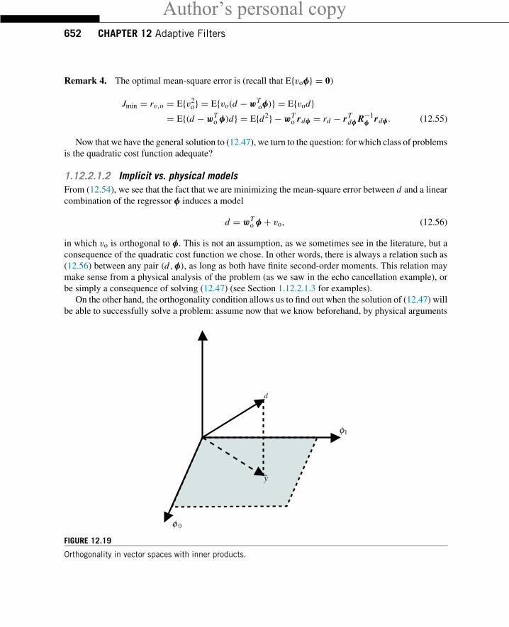
Remark 2. The orthogonality condition is an intuitive result, if we remember that we can think ofthe space of random variables with finite variance as a vector space. In fact, define the cross-correlationrxy = E{xy} between two random variables x and y as the inner product. Then the autocorrelationof a random variable x , E{x2}, would be interpreted as the square of the “length” of x . In this case,our problem (12.47) is equivalent to finding the vector in the subspace spanned by φ0, . . . , φM−1 thatis closest to d . As we know, the solution is such that the error is orthogonal to the subspace. So, theorthogonality condition results from the vector space structure of our problem and the quadratic natureof our cost function. See Figure 12.19.
Remark 3. The difference between (12.54) and the corresponding result obtained in Box 4, Eq. (12.105),is that here the optimum error is orthogonal only to the functions φi of x(n), x(n − 1), . . . that wereincluded in the regressor (and their linear combinations), not to any function, as in (12.105). This is notsurprising: in this section the optimization was made only over the functions in class F , and in Box 4 weallow any function. Both solutions, (12.106) and (12.51), will be equal if the general solution accordingto Box 4 is indeed in F .
Author’s personal copy652 CHAPTER 12 Adaptive Filters
Remark 4. The optimal mean-square error is (recall that E{voφ} = 0)
Jmin = rv,o = E{v2o} = E{vo(d − wT
oφ)} = E{vod}= E{(d − wT
o φ)d} = E{d2} − wTo rdφ = rd − rT
dφ R−1φ rdφ . (12.55)
Now that we have the general solution to (12.47), we turn to the question: for which class of problemsis the quadratic cost function adequate?
1.12.2.1.2 Implicit vs. physical modelsFrom (12.54), we see that the fact that we are minimizing the mean-square error between d and a linearcombination of the regressor φ induces a model
d = wTo φ + vo, (12.56)
in which vo is orthogonal to φ. This is not an assumption, as we sometimes see in the literature, but aconsequence of the quadratic cost function we chose. In other words, there is always a relation such as(12.56) between any pair (d,φ), as long as both have finite second-order moments. This relation maymake sense from a physical analysis of the problem (as we saw in the echo cancellation example), orbe simply a consequence of solving (12.47) (see Section 1.12.2.1.3 for examples).
On the other hand, the orthogonality condition allows us to find out when the solution of (12.47) willbe able to successfully solve a problem: assume now that we know beforehand, by physical arguments
d
φ 0
φ1
y
FIGURE 12.19
Orthogonality in vector spaces with inner products.
Author’s personal copy1.12.2 Optimum Filtering 653
about the problem, that d and φ must be related through
d = wT∗ φ + v, (12.57)
where w∗ is a certain coefficient vector and v is orthogonal to φ. Will the solution to (12.47) be suchthat wo = w∗ and vo = v?
To check if this is the case, we only need to evaluate the cross-correlation vector rdφ assuming themodel (12.57):
rdφ = E{dφ} = E{φ( wT∗ φ︸︷︷︸=φT w∗
+v)} = E{φφT }w∗ + E{φv}︸ ︷︷ ︸=0
= Rφw∗. (12.58)
Therefore, w∗ also obeys the normal equations, and we can conclude that wo = w∗, vo = v, as long asRφ is nonsingular.
Even if Rφ is singular, the optimal error vo will always be equal to v (in a certain sense). In fact, if Rφ
is singular, then there exists a vector a such that Rφa = 0 (see Fact 2 in Box 3), and thus any solutionwo of the normal equations (we know from (12.58) that there is at least one, w∗) will have the form
wo = w∗ + a, a ∈ N (Rφ), (12.59)
where N (Rφ) is the null-space of Rφ . In addition,
0 = aT Rφa = aT E{φφT }a = E{aT φφT a} = E{(aT φ)2
}.
Therefore, aT φ = 0 with probability one. Then,
vo = d − wTo φ = d − (w∗ + a)T φ = d − wT∗ φ,
with probability one. Therefore, although we cannot say that v = vo always, we can say that they areequal with probability one. In other words, when Rφ is singular we may not be able to identify w∗,but (with probability one) we are still able to separate d into its two components. More about this inSection 1.12.2.1.5.
1.12.2.1.3 UndermodelingWe just saw that the solution to the quadratic cost function (12.47) is indeed able to separate the twocomponents of d when the regressor that appears in physical model (12.57) is the same φ that we usedto describe our class F , that is, when our choice of F includes the general solution from Box 4. Let uscheck now what happens when this is not the case.
Assume there is a relationd = wT∗ φe + v, (12.60)
in which v is orthogonal to φe, but our class F is defined through a regressor φ that is a subset of the“correct” one, φe. This situation is called undermodeling: our class is not rich enough to describe thetrue relation between {x(n)} and {d(n)}.
Author’s personal copy654 CHAPTER 12 Adaptive Filters
Assume then that
φe =[
φ
θ
], (12.61)
where φ ∈ RM , θ ∈ RK−M , with K > M . The autocorrelation of φe is
Rφe= E{φeφ
Te } =
[Rφ Rφθ
RTφθ Rθ
],
where Rφθ = E{φθT }. From our hypothesis that φe is orthogonal to v, that is,
0 = E{vφe} =[
E{vφ}E{vθ}
],
we conclude that φ is also orthogonal to v, so
rdφ = E{φ(φT
e w∗ + v)}= E{φφT
e }w∗ + E{φv}︸ ︷︷ ︸=0
= [Rφ Rφθ
]w∗.
Assuming that Rφ is nonsingular, solving the normal Eq. (12.50) we obtain
wo = R−1φ
[Rφ Rφθ
]w∗ =
[I R−1
φ Rφθ
]w∗. (12.62)
Now we have two interesting special cases: first, if φ and θ are orthogonal, i.e., if Rφθ = 0, then wocontains the first M elements of w∗. Let us consider a specific example: assume that
φ =
⎡⎢⎢⎢⎣x(n)
x(n − 1)...
x(n − M + 1)
⎤⎥⎥⎥⎦ , but φe =
⎡⎢⎢⎢⎣x(n)
x(n − 1)...
x(n − K + 1)
⎤⎥⎥⎥⎦ , (12.63)
with M < K . Then θ = [x(n − M) . . . x(n − K + 1)
]T . This situation is very common in practice.In this case, Rφθ = 0 when {x(n)} is zero-mean white noise. This is one reason why white noise is
the preferred input to be used in system identification: even in the (very likely in practice) case in whichM < K , at least the first elements of w∗ are identified without bias.
On the other hand, if Rφθ = 0, then wo is a mixture of the elements of w∗. This happens in (12.63)when the input sequence {x(n)} is not white. In this case, the optimum filter wo takes advantage of thecorrelation between the entries of φ and θ to estimate θ given φ, and uses these estimated values toobtain a better approximation for d . Sure enough, if you write down the problem of approximating θ
linearly from φ, namely,
Wo = arg minW
E
{∥∥∥θ −W T φ
∥∥∥2},
you will see that the solution is exactly Wo = R−1φ Rφθ .
Author’s personal copy1.12.2 Optimum Filtering 655
What is important to notice is that in both cases the optimum error vo is not equal to v:
vo = d − wTo φ = wT∗ φe + v − wT
o φ.
Partitioning w∗ =[wT∗,1 wT∗,2
]T, with w∗,1 ∈ RM ,w∗,2 ∈ RK−M , we have
vo =(w∗,1 − wo
)Tφ + wT∗,2θ + v = wT∗,2 RT
φθ R−1φ φ + wT∗,2θ + v
= wT∗,2(θ − RT
φθ R−1φ φ
)+ v.
Although vo = v, you may check that indeed E{voφ} = 0.As another example, assume that we have two variables such that d = ax + bx3 + v, in which v
has zero mean and is independent of x , and a and b are constants. Assume that we choose as regressorsimply φ = x , so we try to solve
wo = arg minw
E{(d − wx)2
}.
In this case we haveRφ = E{x2}, rdφ = E{xd} = E{ax2 + bx4},
since E{xkv} = E{xk}E{v} = 0. The optimum solution is thus
wo = aE{x2} + bE{x4}E{x2} ,
and the optimum error is
vo = d − wox = ax + bx3 + v − aE{x2} + bE{x4}E{x2} x = v + b
(x2 − E{x4}
E{x2})
x = v.
However, vo is again orthogonal to x (but not to x3, which we did not include in the regressor).What happens in the opposite situation, when we include more entries in φ than necessary? As one
would expect, in this case the parameters related to these unnecessary entries will be zeroed in theoptimum solution wo. This does not mean, however, that we should hasten to increase φ to make F aslarge as possible, and leave to the filter the task of zeroing whatever was not necessary. This is becauseincreasing the number of parameters to be estimated has a cost. The first and more obvious cost is interms of memory and number of computations. However, we saw in Section 1.12.1.2 that an actualadaptive filter usually does not converge to the exact optimum solution, but rather hovers around it.Because of this, increasing the number of parameters may in fact decrease the quality of the solution.We explain this in more detail in Section 1.12.4.
1.12.2.1.4 Zero and non-zero mean variablesUp to now we did not assume anything about the means of d and φ. If both d and φ have zero mean,we can interpret all autocorrelations as variances or covariance matrices, according to the case. To seethis, assume that
E{d} = 0, E{φ} = 0. (12.64)
Author’s personal copy656 CHAPTER 12 Adaptive Filters
Then E{y} = E{wTo φ} = 0, and thus
E{vo} = E{d} − wTo E{φ} = 0+ wT
o 0 = 0,
so the optimum error has zero mean. In this case, rd = E{d2} = σ 2d is the variance of d, and E{v2
o} = σ 2v,o
is the variance of vo, so (12.55) becomes
Jmin = σ 2v,o = E{v2
o} = σ 2d − rT
dφ R−1φ rdφ . (12.65)
Since Rφ is positive-definite, we conclude that the uncertainty in vo (its variance) is never larger thanthe uncertainty in d (Box 3).
However, vo may have a nonzero mean if either d or φ has nonzero mean. This is verified as follows.Define
d = E{d}, φ = E{φ}, (12.66)
then
E{vo} = E{d − rTdφ R−1
φ φ} = d − rTdφ R−1
φ φ = 0
in general (for example, if φ = 0, but d = 0).In many applications, vo should approximate some signal that is constrained to have zero mean, such
as speech or noise, or because vo will be passed through a system with a high DC gain (such as anintegrator), so it may be useful to guarantee that vo has zero mean. How can this be done if the means ofd and φ are not zero? This problem is quite common, particularly when φ includes nonlinear functionsof x(n). Fortunately, there are two easy solutions: First, if one knew the means of d and φ, one coulddefine zero-mean variables
dc = d − E{d}, φc = φ − E{φ}, (12.67)
and use them instead of the original variables in (12.47). This is the simplest solution, but we often donot know the means d and φ.
The second solution is used when the means are not known: simply add an extra term to φ, definingan extended regressor (not to be confused with the extended regressor from Section 1.12.2.1.3)
φe =[
1φ
], (12.68)
and an extended weight vector we ∈ RM+1. The first coefficient of we will take care of the means, aswe show next. The extended cross-correlation vector and autocorrelation matrix are
rdφe=[
drdφ
], Rφe
=[
1 φT
φ Rφ
].
Author’s personal copy1.12.2 Optimum Filtering 657
Assuming that Rφeand Rφ are nonsingular, we can compute wo,e if we evaluate the inverse of Rφe
using Schur complements (See Fact 3 in Box 3), as follows
wo,e = R−1φe
rdφe
=[
1 0T
−R−1φ φ I
][(1− φ
TR−1
φ φ)−1 0T
0 R−1φ
][1 −φ
TR−1
φ
0 I
][d
rdφ
]
=[
1 0T
−R−1φ φ I
][(1− φ
TR−1
φ φ)−1 0T
0 R−1φ
][d − φ
TR−1
φ rdφ
rdφ
]
=[
1 0T
−R−1φ φ I
]⎡⎢⎣ d−φT
R−1φ rdφ
1−φT
R−1φ φ
R−1φ rdφ
⎤⎥⎦ =⎡⎢⎢⎣
d−φT
R−1φ rdφ
1−φT
R−1φ φ
R−1φ rdφ − d−φ
TR−1
φ rdφ
1−φT
R−1φ φ
R−1φ φ
⎤⎥⎥⎦ .Using this result, we can evaluate now E{vo,e} = E{d} − wT
o,eE{φe} as follows (we used the fact thatthe inverse of a symmetric matrix is also symmetric from Box 3):
E{vo,e} = d − d − φT
R−1φ rdφ
1− φT
R−1φ φ
− rTdφ R−1
φ φ + d − φT
R−1φ rdφ
1− φT
R−1φ φ
φT
R−1φ φ
= d − rTdφ R−1
φ φ − d − φT
R−1φ rdφ
1− φT
R−1φ φ
(1− φ
TR−1
φ φ)= 0.
1.12.2.1.5 Sufficiently rich signalsWe saw in Section 1.12.2.1.2 that even when Rφ is singular, we can recover the optimum vo (withprobability one), but not the optimum w∗. Let us study this problem in more detail, since it is importantfor system identification. So, what does it mean in practice to have a singular autocorrelation functionRφ? The answer to this question can be quite complicated when the input signals are nonstationary(i.e., when Rφ is not constant), so in this case we refer the interested reader to texts in adaptive control(such as [18]), which treat this problem in detail (although usually from a deterministic point of view).We consider here only the case in which the signals {d(n), x(n)} are jointly wide-sense stationary.
In this case, Rφ may be singular because some entries of φ are linear combinations of the others.For example, if we choose φ0 = x(n) and φ1 = 2x(n), then
Rφ = E{x2(n)}[
1 22 4
],
which is singular.However, there are more subtle ways in which Rφ may become singular. Assume for example that
our input sequence is given byx(n) = cos (ω0n + ϕ), (12.69)
Author’s personal copy658 CHAPTER 12 Adaptive Filters
where 0 < ω0 ≤ π is the frequency, and ϕ is a random phase, uniformly distributed in the interval[0, 2π). This kind of model (sinusoidal signals with random phases), by the way, is the bridge betweenthe periodic signals from Section 1.12.1.2 and the stochastic models discussed in this section. In thiscase, consider a vector φ formed from a delay line with x(n) as input,
φ = [ x(n) x(n − 1) . . . x(n − M + 1) ]T .If M = 2, we have
Rφ =[
E{x2(n)} E{x(n)x(n − 1)}E{x(n)x(n − 1)} E{x2(n − 1)}
]= 1
2
[1 cos (ω0)
cos (ω0) 1
].
The determinant of Rφ is 1− cos2 (ω0) = sin2 (ω0) = 0 if ω0 = 0 and ω0 = π .However, for any M ≥ 3, the resulting Rφ will be singular: we can write
φ = 1
2e j(ω0n+ϕ)
⎡⎢⎢⎢⎣1
e− jω0
...
e− j(M−1)ω0
⎤⎥⎥⎥⎦+ 1
2e− j(ω0n+ϕ)
⎡⎢⎢⎢⎣1
e jω0
...
e j(M−1)ω0
⎤⎥⎥⎥⎦ ,and since E{(e jω0n+ jϕ)2} = E{e j2(ω0n+ϕ)} = 0,E{e j(ω0n+ϕ)e− j(ω0n+ϕ)} = 1, we have
Rφ = 1
4
⎡⎢⎢⎢⎣1
e− jω0
...
e− j(M−1)ω0
⎤⎥⎥⎥⎦[1 e jω0 . . . e j(M−1)ω0
]
+1
4
⎡⎢⎢⎢⎣1
e jω0
...
e j(M−1)ω0
⎤⎥⎥⎥⎦[1 e− jω0 . . . e− j(M−1)ω0
].
Since Rφ is the sum of two rank-one matrices, its rank is at most two. It will be two when 0 < ω0 < π ,since in this case the vectors are linearly independent. We conclude that when the input signal is a sinusoidas in (12.69), the optimum solution to (12.47) will never be able to identify more than two coefficients.This argument can be generalized: if x(n) is composed of K sinusoids of different frequencies, thenRφ will be nonsingular if and only if M ≤ 2K .
The general conclusion is that Rφ will be singular or not, depending on which functions are chosenas inputs, and on the input signal. We say that the input is sufficiently rich for a given problem if it issuch that Rφ is nonsingular. We show a few examples next.
1.12.2.1.6 ExamplesThe concepts we saw in Sections 1.12.2.1.2–1.12.2.1.5 can be understood intuitively if we return to ourexample in Section 1.12.1.2. In that example, the true echo was obtained by filtering the input x(n) by
Author’s personal copy1.12.2 Optimum Filtering 659
an unknown H(z), so we had
d(n) =K∑
k=0
hk x(n − k)+ v(n),
where K is the true order of the echo path, v(n) = B cos (ω1n + θ) and x(n) = A cos (ω0n + ϕ). Weconsidered only one harmonic for simplicity.
We are trying to cancel the echo, by constructing an approximated transfer function H(z), which ismodeled as an FIR filter with M coefficients. As we saw in Section 1.12.1.2, if x(n) is a simple sinusoid,the echo will be completely canceled if we satisfy (12.8), reproduced below
Re{H(e jω0)} = Re{H(e jω0)}, Im{H(e jω0)} = Im{H(e jω0)}.If K = M = 1, so H(z) = h0 + h1z−1 and H(z) = w0 + w1z−1, this condition becomes
w0 + w1 cos (−ω0) = h0 + h1 cos (−ω0),
w1 sin (−ω0) = h1 sin (−ω0),
with a single solution w0 = h0, w1 = h1.On the other hand, if the input were as before (a single sinusoid), but K = 2, so H(z) = h0 +
h1z−1 + h2z−2, the equations would be
w0 + w1 cos (−ω0) = h0 + h1 cos (−ω0)+ h2 cos (−2ω0),
w1 sin (−ω0) = h1 sin (−ω0)+ h2 sin (−2ω0),
and the solution would be unique (since Rφ is nonsingular), but would not approximate h0 and h1 ingeneral.
This is an example of an undermodeled system, as we saw in Section 1.12.2.1.3. Figure 12.20shows the LMS algorithm derived in Section 1.12.1.2 applied to this problem. Note that, even thoughw0(n), w1(n) do not converge to h0, h1, in this example the error e(n) does approximate well v(n). Thishappens because in this case x(n) is periodic, and the term x(n− 2) can be obtained exactly as a linearcombination of x(n) and x(n− 1) (Check that using the expressions for v0 from Section 1.12.2.1.3, weobtain v0 = v in this case.)
If we tried to identify H(z) by adding an extra coefficient to H(z), the equations would be
w0 + w1 cos (−ω0)+ w2 cos (−2ω0) = h0 + h1 cos (−ω0)+ h2 cos (−2ω0),
w1 sin (−ω0)+ w2 sin (−2ω0) = h1 sin (−ω0)+ h2 sin (−2ω0). (12.70)
Now w0 = h0, w1 = h1, and w2 = h2 is a solution, but not the only one. Depending on the initialcondition, the filter would converge to a different solution, as can be seen in Figure 12.21 (the levelsets are not shown, because they are not closed curves in this case). The input is not rich enough (inharmonics) to excite the unknown system H(z) so that the adaptive filter might identify it, as we sawin Section 1.12.2.1.5. However, for all solutions the error converges to v(n).
If the input had a second harmonic (K0 = 2), we would add two more equations to (12.70), cor-responding to H(e2 jω0) = H(e2 jω0), and the filter would be able to identify systems with up to fourcoefficients.
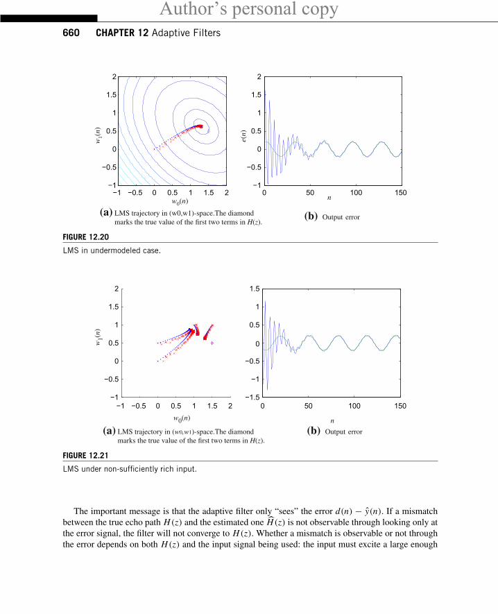
Author’s personal copy660 CHAPTER 12 Adaptive Filters
−1 −0.5 0 0.5 1 1.5 2−1
−0.5
0
0.5
1
1.5
2
w0(n)
w1(
n)
(a) LMS trajectory in (w0,w1)-space.The diamond marks the true value of the first two terms in H(z).
0 50 100 150−1
−0.5
0
0.5
1
1.5
2
n
e(n)
(b) Output error
FIGURE 12.20
LMS in undermodeled case.
−1 −0.5 0 0.5 1 1.5 2−1
−0.5
0
0.5
1
1.5
2
w0(n)
w1(n
)
(a) LMS trajectory in (w0,w1)-space.The diamond marks the true value of the first two terms in H(z).
0 50 100 150−1.5
−1
−0.5
0
0.5
1
1.5
n
(b) Output error
FIGURE 12.21
LMS under non-sufficiently rich input.
The important message is that the adaptive filter only “sees” the error d(n) − y(n). If a mismatchbetween the true echo path H(z) and the estimated one H(z) is not observable through looking only atthe error signal, the filter will not converge to H(z). Whether a mismatch is observable or not throughthe error depends on both H(z) and the input signal being used: the input must excite a large enough
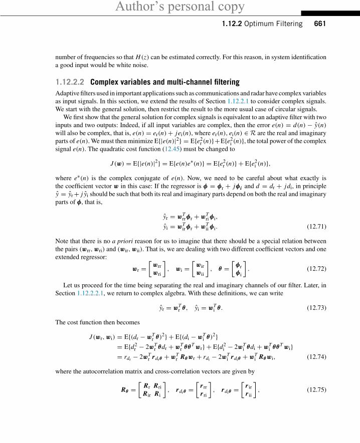
Author’s personal copy1.12.2 Optimum Filtering 661
number of frequencies so that H(z) can be estimated correctly. For this reason, in system identificationa good input would be white noise.
1.12.2.2 Complex variables and multi-channel filteringAdaptive filters used in important applications such as communications and radar have complex variablesas input signals. In this section, we extend the results of Section 1.12.2.1 to consider complex signals.We start with the general solution, then restrict the result to the more usual case of circular signals.
We first show that the general solution for complex signals is equivalent to an adaptive filter with twoinputs and two outputs: Indeed, if all input variables are complex, then the error e(n) = d(n) − y(n)will also be complex, that is, e(n) = er(n)+ jei(n), where er(n), ei(n) ∈ R are the real and imaginaryparts of e(n). We must then minimize E{|e(n)|2} = E{e2
r (n)}+E{e2i (n)}, the total power of the complex
signal e(n). The quadratic cost function (12.45) must be changed to
J (w) = E{|e(n)|2} = E{e(n)e∗(n)} = E{e2r (n)} + E{e2
i (n)},where e∗(n) is the complex conjugate of e(n). Now, we need to be careful about what exactly isthe coefficient vector w in this case: If the regressor is φ = φr + jφ i and d = dr + jdi, in principley = yr+ j yi should be such that both its real and imaginary parts depend on both the real and imaginaryparts of φ, that is,
yr = wTrrφr + wT
ri φi,
yi = wTir φr + wT
ii φi. (12.71)
Note that there is no a priori reason for us to imagine that there should be a special relation betweenthe pairs (wrr,wri) and (wir,wii). That is, we are dealing with two different coefficient vectors and oneextended regressor:
wr =[
wrrwri
], wi =
[wirwii
], θ =
[φrφi
]. (12.72)
Let us proceed for the time being separating the real and imaginary channels of our filter. Later, inSection 1.12.2.2.1, we return to complex algebra. With these definitions, we can write
yr = wTr θ , yi = wT
i θ . (12.73)
The cost function then becomes
J (wr,wi) = E{(dr − wTr θ)2} + E{(di − wT
i θ)2}= E{d2
r − 2wTr θdr + wT
r θθT wr} + E{d2i − 2wT
i θdi + wTi θθT wi}
= rdr − 2wTr rdrθ + wT
r Rθwr + rdi − 2wTi rdiθ + wT
i Rθwi, (12.74)
where the autocorrelation matrix and cross-correlation vectors are given by
Rθ =[
Rr RriRir Ri
], rdrθ =
[r rrr ri
], rdiθ =
[r irr ii
], (12.75)
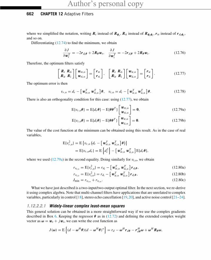
Author’s personal copy662 CHAPTER 12 Adaptive Filters
where we simplified the notation, writing Rr instead of Rφr, Rri instead of Rφrφi
, r rr instead of rdrφr,
and so on.Differentiating (12.74) to find the minimum, we obtain
∂ J
∂wTr= −2rdrθ + 2Rθwr,
∂ J
∂wTi
= −2rdiθ + 2Rθwi. (12.76)
Therefore, the optimum filters satisfy[Rr RriRir Ri
] [wrr,owri,o
]=[
r rrr ri
],
[Rr RriRir Ri
] [wir,owii,o
]=[
r irr ii
]. (12.77)
The optimum error is then
vr ,o = dr −[wT
rr,o wTri,o
]θ , vi,o = di −
[wT
ir,o wTii,o
]θ . (12.78)
There is also an orthogonality condition for this case: using (12.77), we obtain
E{vr ,oθ} = E{drθ} − E{θθT }[
wrr,owri,o
]= 0, (12.79a)
E{vi,oθ} = E{diθ} − E{θθT }[
wir,owii,o
]= 0. (12.79b)
The value of the cost function at the minimum can be obtained using this result. As in the case of realvariables,
E{v2r ,o} = E
{vr ,o
(dr −
[wT
rr,o wTri,o
]θ)}
= E{vr ,odr } = E{
d2r
}− [
wTrr,o wT
ri,o
]E{drθ},
where we used (12.79a) in the second equality. Doing similarly for vi,o, we obtain
rvr,o = E{v2r ,o} = rdr −
[wT
rr,o wTri,o
]rdrθ , (12.80a)
rvi,o = E{v2i,o} = rdi −
[wT
ir,o wTii,o
]rdi θ , (12.80b)
Jmin = rvr,o + rvi,o . (12.80c)
What we have just described is a two-input/two-output optimal filter. In the next section, we re-deriveit using complex algebra. Note that multi-channel filters have applications that are unrelated to complexvariables, particularly in control [18], stereo echo cancellation [19,20], and active noise control [21–24].
1.12.2.2.1 Widely-linear complex least-mean squaresThis general solution can be obtained in a more straightforward way if we use the complex gradientsdescribed in Box 6. Keeping the regressor θ as in (12.72) and defining the extended complex weightvector as ω = wr + jwi, we can write the cost function as
J (ω) = E{(d − ωH θ)(d − ωH θ)∗
}= rd − ωH rdθ − r H
dθω + ωH Rθω,
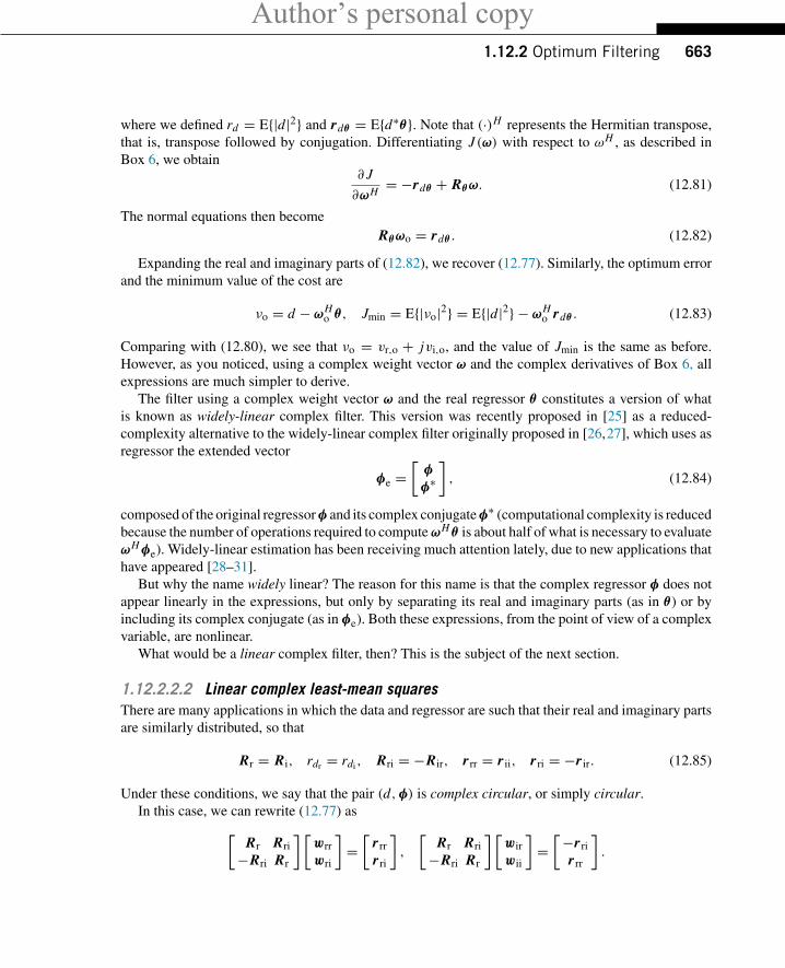
Author’s personal copy1.12.2 Optimum Filtering 663
where we defined rd = E{|d|2} and rdθ = E{d∗θ}. Note that (·)H represents the Hermitian transpose,that is, transpose followed by conjugation. Differentiating J (ω) with respect to ωH , as described inBox 6, we obtain
∂ J
∂ωH= −rdθ + Rθω. (12.81)
The normal equations then becomeRθωo = rdθ . (12.82)
Expanding the real and imaginary parts of (12.82), we recover (12.77). Similarly, the optimum errorand the minimum value of the cost are
νo = d − ωHo θ , Jmin = E{|νo|2} = E{|d|2} − ωH
o rdθ . (12.83)
Comparing with (12.80), we see that νo = vr,o + jvi,o, and the value of Jmin is the same as before.However, as you noticed, using a complex weight vector ω and the complex derivatives of Box 6, allexpressions are much simpler to derive.
The filter using a complex weight vector ω and the real regressor θ constitutes a version of whatis known as widely-linear complex filter. This version was recently proposed in [25] as a reduced-complexity alternative to the widely-linear complex filter originally proposed in [26,27], which uses asregressor the extended vector
φe =[
φ
φ∗], (12.84)
composed of the original regressor φ and its complex conjugate φ∗ (computational complexity is reducedbecause the number of operations required to compute ωH θ is about half of what is necessary to evaluateωH φe). Widely-linear estimation has been receiving much attention lately, due to new applications thathave appeared [28–31].
But why the name widely linear? The reason for this name is that the complex regressor φ does notappear linearly in the expressions, but only by separating its real and imaginary parts (as in θ ) or byincluding its complex conjugate (as in φe). Both these expressions, from the point of view of a complexvariable, are nonlinear.
What would be a linear complex filter, then? This is the subject of the next section.
1.12.2.2.2 Linear complex least-mean squaresThere are many applications in which the data and regressor are such that their real and imaginary partsare similarly distributed, so that
Rr = Ri, rdr = rdi , Rri = −Rir, r rr = r ii, r ri = −r ir. (12.85)
Under these conditions, we say that the pair (d,φ) is complex circular, or simply circular.In this case, we can rewrite (12.77) as[
Rr Rri−Rri Rr
] [wrrwri
]=[
r rrr ri
],
[Rr Rri−Rri Rr
] [wirwii
]=[−r ri
r rr
].
Author’s personal copy664 CHAPTER 12 Adaptive Filters
Expand these equations as follows (notice the change in order in (12.86b))
Rrwrr + Rriwri = r rr, −Rriwrr + Rrwri = r ri, (12.86a)
Rrwii − Rriwir = r rr, Rriwii + Rrwir = −r ri. (12.86b)
Now we can see that, if (wrr,wri) is a solution to (12.86a), then
(wii = wrr,wir = −wri) (12.87)
is a solution to (12.86b). Therefore, when the input signals are circular, the number of degrees of freedomin the problem is actually smaller. In this case, there is a very nice way of recovering the solutions,working only with complex algebra. Indeed, defining w = wrr + jwri, we have
wH φ = (wrr − jwri)T (φr + jφi)
=(wT
rrφr + wTri φi
)+ j
(wT
rrφi − wTri φr
), (12.88)
which is equivalent to (12.71) with the identities (12.87). Using this definition, it is possible to obtainthe optimum solution (12.86a), (12.86b), and (12.87) using only complex algebra, following exactlythe same steps as our derivation for the real case in the previous section.
This path is very useful, we can derive almost all results for real or complex circular adaptive filtersusing the same arguments. Let us see how it goes. First, define y = wH φ, so our problem becomes
minw∈CM
E
{∣∣∣d − wH φ
∣∣∣2} . (12.89)
Expanding the cost, recalling that now∣∣d − wH φ
∣∣2 = (d −wH φ)(d −wH φ)∗ = (d −wH φ)(d∗ −φH w), we obtain
J (w) = E{|d|2 − wH φd∗ − dφH w + wH φφH w
}= rd − wH rdφ − r H
dφw + wH Rφw, (12.90)
where we defined rd = E{|d|2}, rdφ = E{d∗φ}, Rφ = E{φφH }.We need to find the minimum of this cost.One easy solution is to use the rules for differentiation of
real functions of complex variables, as described in Box 6. These rules are very useful, and surprisinglyeasy to use: basically, we can treat w and its conjugate wH as if they were independent variables, that is
∂ J
∂wH= −rdφ + Rφw. (12.91)
Equating the gradient to zero, the solution is (assuming that Rφ is nonsingular)
wo = R−1φ rdφ, (12.92)
which is exactly equal to (12.51). This is the advantage of this approach: the expressions for complexand real problems are almost equal. The important differences are the conjugates that appear in the
Author’s personal copy1.12.2 Optimum Filtering 665
definitions of Rφ and rdφ , and the absence of a factor of 2 in the gradient (12.91). This follows fromthe definition of complex derivative we used (see Box 6). Here this difference is canceled out in thesolution (12.92), but further on we will find situations in which there will be a different factor for thecase of real and for the case of complex variables.
Let us check that (12.92) is really equivalent to (12.86a). Expanding Rφ and rdφ and using thecircularity conditions (12.85), we obtain
Rφ = E{φφH } = E{(φr + jφi)(φr − jφi)T } = Rr + Ri + j
(Rir − Rri
), (12.93a)
= 2Rr − 2 j Rri, (12.93b)
and
rdφ = E{d∗φ} = E{(dr − jdi)(φr + jφi)} = r rr + r ii + j(r ri − r ir
)= 2r rr + 2 j r ri, (12.94)
so, equating the gradient (12.91) to zero, wo = wr,o + jwi,o must satisfy
2(
Rr − j Rri) (
wr,o + jwi,o) = 2
(r rr + j r ri
),
Rrwr,o + Rriwi,o + j(
Rrwi,o − Rriwr,o) = r rr + j r ri. (12.95)
Comparing the real and imaginary parts of (12.95) with (12.86a), we see that they indeed correspondto the same set of equations.
A few important remarks:
Remark 5. The orthogonality condition still holds in the complex circular case, but with a smalldifference: defining the optimum error as before,
vo = d − wHo φ,
we obtain, noting that (wHo φ)∗ = φH wo,
E{v∗oφ} = E{d∗φ − φφH wo} = rdφ − Rφwo = 0. (12.96)
Remark 6. The complex gradient (12.91) seems strange because it does not include the factors of 2that would appear in the real case. This difference will appear in many expressions in the followingsections, whenever we need to differentiate between the real and complex cases. However, the differenceis illusory: if you go back to (12.93b) and (12.94), you will see that the factor of two is actually there,just hidden by the definition of autocorrelation and cross-correlation under the circularity conditions.
Remark 7. The optimum error power can be obtained as in the real case, and is equal to
E{|vo|2} = rd − wHo rdφ = rd − r H
dφ R−1φ rdφ . (12.97)
Author’s personal copy666 CHAPTER 12 Adaptive Filters
Box 4: Least mean-squares estimation
Here we consider the general problem of finding the optimum relation Ho between d(n) and x(n),such that
Ho = arg minH
E{
d(n)− H(x(n), x(n − 1), . . . )}, (12.98)
without restricting H to a particular class.In order to understand well this problem, let us consider first the simpler case where the relation
between x(n) and d(n) is memoryless, that is, our function depends only on the current value of x(n).Dropping the time index to simplify the notation, our problem then becomes how to find a functionH that, applied to a certain random variable x , approximates a certain random variable d so that themean-square error is minimized, that is, we want to solve
minH
E{[d − H(x)]2}. (12.99)
Assume that the joint probability density function pdx (d, x) of d and x is known (we are assumingthat d and x are continuous random variables, but the final result in (12.100) also holds if they arediscrete). Then,
E{[d − H(x)]2} =∫ ∫[d − H(x)]2 pdx (d, x)d d dx
=∫ {∫
[d − H(x)]2 pd|x (d|x)d d
}︸ ︷︷ ︸
Ed {[d−H(x)]2|x}
px (x)dx
= Ex
{Ed
{[d − H(x)]2|x
}}, (12.100)
where we use the subscripts Ed and Ex to highlight that the expectations are taken with respect to d orx only.
Note that the inner integrand Ed{[d−H(x)]2|x} in (12.100) is nonnegative. Therefore, if we minimizeit for each value of x , we will obtain the minimum of the full expression. That is, the optimum Ho isthe function defined by
Ho(x) = arg minH(x)
Ed
{[d − H(x)]2|x
}. (12.101)
It is important to remember that, fixed x, H(x) is simply a number. This can be seen more easilyexpanding the expectations in (12.101)
Ed
{[d − H(x)]2|x
}=
∫ (d2 − 2dH(x)+ H2(x)
)pd|x (d|x)dd
=∫
d2 pd|x (d|x)dd − 2H(x)∫
dpd|x (d|x)dd + H2(x)∫
pd|x (d|x)dd
= Ed{d2|x} − 2E{d|x}H(x)+ H2(x).
Author’s personal copy1.12.2 Optimum Filtering 667
Differentiating with respect to H(x) and equating to zero, we obtain the solution
Ho(x) = Ed{d|x} �= y(n), (12.102)
which is indeed a function of x , as desired.Let us study the properties of this solution. First, define
vo = d − Ho(x).
Note that vo and Ho are not necessarily equal to v and H from (12.40). Evaluating the average of Ho(x),we obtain
Ex {Ho(x)} = Ex {Ed{d|x}} = E{d},by an argument similar to that used to obtain (12.100). We conclude that vo has zero mean. In addition,for any function f (x) of x for which the expected values exist, we have
E{vo f (x)} = Ex {Ed{d f (x)}} − E {Ed{d|x} f (x)} = 0 = E{vo}E{ f (x)}, (12.103)
since Ed{d f (x)|x} = f (x)Ed{d|x}. This result means that the error vo is uncorrelated to any functionof the reference data x , which is a very strong condition. It basically means that we have extracted allsecond-order information available in x about d.
We remark that (12.103) does not imply that x and vo are independent. A simple counter-example isthe following: consider two discrete-valued random variables r and s with joint probabilities given byTable 12.1. Then E{s f (r)} = 1/4 · (−1) · f (+ 1)+ 1/4 · (+ 1) · f (+ 1)+ 1/2 · 0 · f (−1) = 0,∀ f (·),but r and s are not independent.
In the more general case in which H is allowed to depend on previous samples of x(n), the argumentsand the final conclusion are similar:
arg minH
E
{[d − H(x(n), x(n − 1), . . . )
]2}= E {d| x(n), x(n − 1), . . .} , (12.104)
and defining
vo(n) = d(n)− E {d | x(n), x(n − 1), . . .} ,
Table 12.1 Counter-Example: (12.103) does not Imply Independence
r \ s −1 0 1
−1 0 1/2 01 1/4 0 1/4
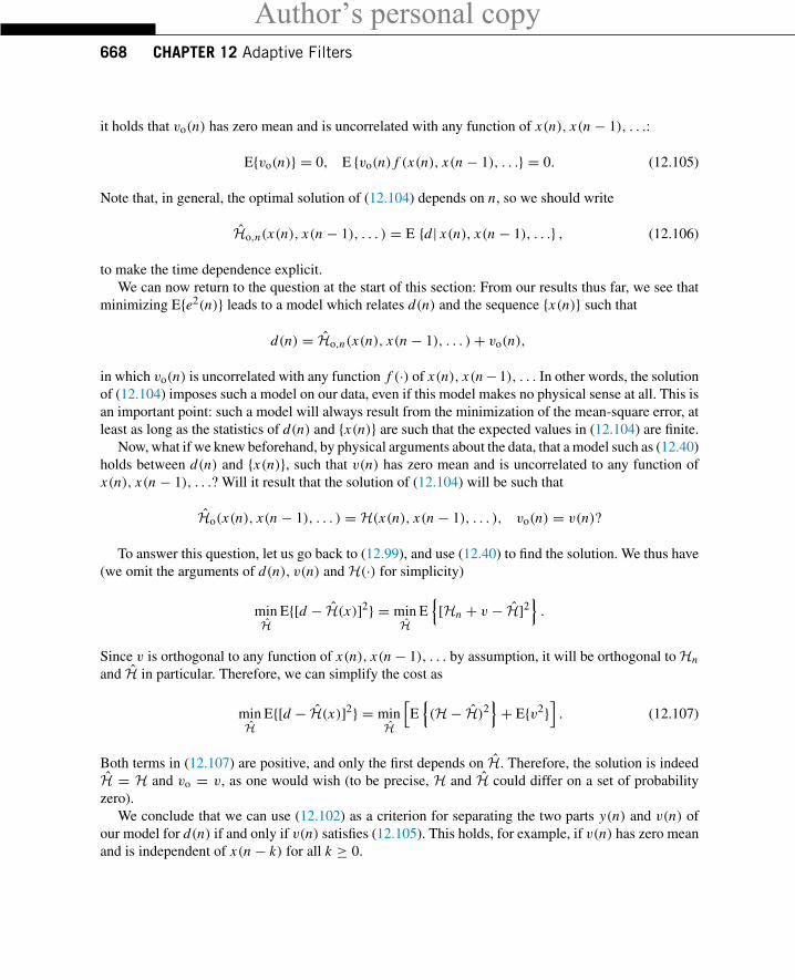
Author’s personal copy668 CHAPTER 12 Adaptive Filters
it holds that vo(n) has zero mean and is uncorrelated with any function of x(n), x(n − 1), . . .:
E{vo(n)} = 0, E {vo(n) f (x(n), x(n − 1), . . .} = 0. (12.105)
Note that, in general, the optimal solution of (12.104) depends on n, so we should write
Ho,n(x(n), x(n − 1), . . . ) = E {d| x(n), x(n − 1), . . .} , (12.106)
to make the time dependence explicit.We can now return to the question at the start of this section: From our results thus far, we see that
minimizing E{e2(n)} leads to a model which relates d(n) and the sequence {x(n)} such that
d(n) = Ho,n(x(n), x(n − 1), . . . )+ vo(n),
in which vo(n) is uncorrelated with any function f (·) of x(n), x(n−1), . . . In other words, the solutionof (12.104) imposes such a model on our data, even if this model makes no physical sense at all. This isan important point: such a model will always result from the minimization of the mean-square error, atleast as long as the statistics of d(n) and {x(n)} are such that the expected values in (12.104) are finite.
Now, what if we knew beforehand, by physical arguments about the data, that a model such as (12.40)holds between d(n) and {x(n)}, such that v(n) has zero mean and is uncorrelated to any function ofx(n), x(n − 1), . . .? Will it result that the solution of (12.104) will be such that
Ho(x(n), x(n − 1), . . . ) = H(x(n), x(n − 1), . . . ), vo(n) = v(n)?
To answer this question, let us go back to (12.99), and use (12.40) to find the solution. We thus have(we omit the arguments of d(n), v(n) and H(·) for simplicity)
minH
E{[d − H(x)]2} = minH
E{[Hn + v − H]2
}.
Since v is orthogonal to any function of x(n), x(n − 1), . . . by assumption, it will be orthogonal to Hn
and H in particular. Therefore, we can simplify the cost as
minH
E{[d − H(x)]2} = minH
[E{(H− H)2
}+ E{v2}
]. (12.107)
Both terms in (12.107) are positive, and only the first depends on H. Therefore, the solution is indeedH = H and vo = v, as one would wish (to be precise, H and H could differ on a set of probabilityzero).
We conclude that we can use (12.102) as a criterion for separating the two parts y(n) and v(n) ofour model for d(n) if and only if v(n) satisfies (12.105). This holds, for example, if v(n) has zero meanand is independent of x(n − k) for all k ≥ 0.
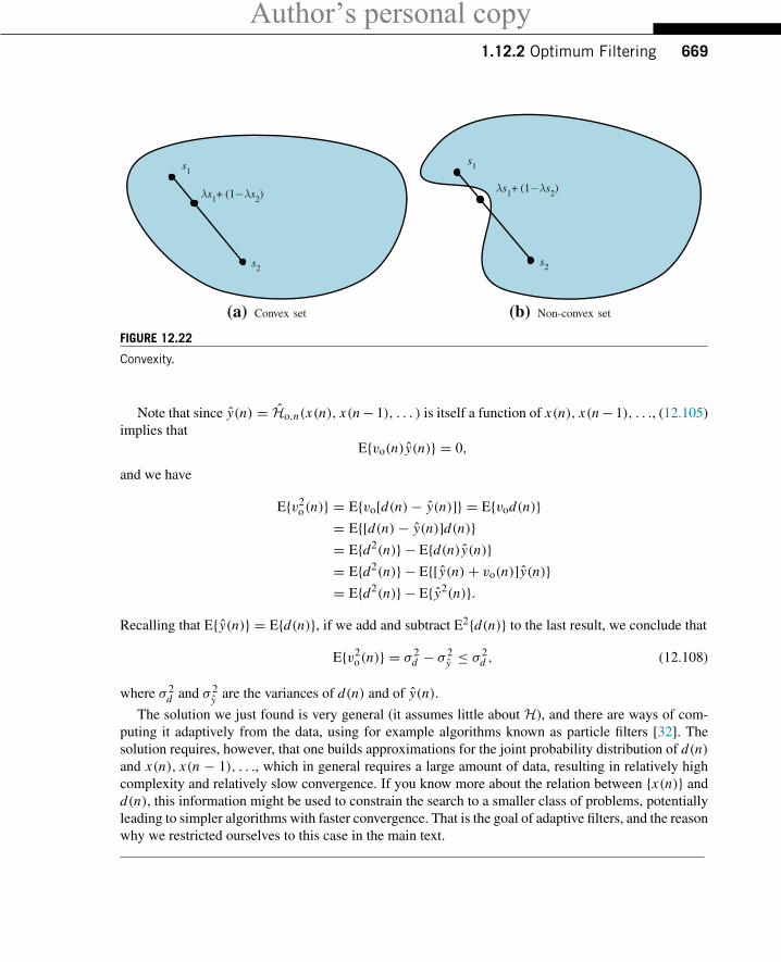
Author’s personal copy1.12.2 Optimum Filtering 669
s1
s2
λs1+ (1−λs2)
(a) Convex set
s1
s2
λs1+ (1−λs2)
(b) Non-convex set
FIGURE 12.22
Convexity.
Note that since y(n) = Ho,n(x(n), x(n− 1), . . . ) is itself a function of x(n), x(n− 1), . . ., (12.105)implies that
E{vo(n)y(n)} = 0,
and we have
E{v2o(n)} = E{vo[d(n)− y(n)]} = E{vod(n)}
= E{[d(n)− y(n)]d(n)}= E{d2(n)} − E{d(n)y(n)}= E{d2(n)} − E{[y(n)+ vo(n)]y(n)}= E{d2(n)} − E{y2(n)}.
Recalling that E{y(n)} = E{d(n)}, if we add and subtract E2{d(n)} to the last result, we conclude that
E{v2o(n)} = σ 2
d − σ 2y ≤ σ 2
d , (12.108)
where σ 2d and σ 2
y are the variances of d(n) and of y(n).
The solution we just found is very general (it assumes little about H), and there are ways of com-puting it adaptively from the data, using for example algorithms known as particle filters [32]. Thesolution requires, however, that one builds approximations for the joint probability distribution of d(n)and x(n), x(n − 1), . . ., which in general requires a large amount of data, resulting in relatively highcomplexity and relatively slow convergence. If you know more about the relation between {x(n)} andd(n), this information might be used to constrain the search to a smaller class of problems, potentiallyleading to simpler algorithms with faster convergence. That is the goal of adaptive filters, and the reasonwhy we restricted ourselves to this case in the main text.
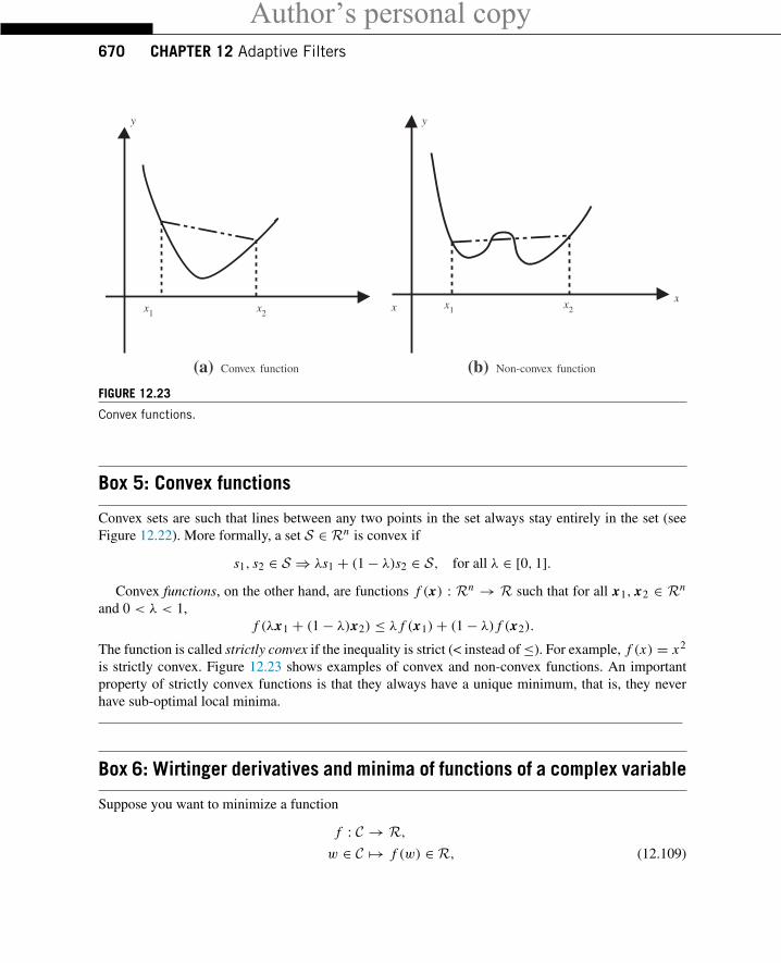
Author’s personal copy670 CHAPTER 12 Adaptive Filters
x1 x2x
y
(a) Convex function
x1 x2x
y
(b) Non-convex function
FIGURE 12.23
Convex functions.
Box 5: Convex functions
Convex sets are such that lines between any two points in the set always stay entirely in the set (seeFigure 12.22). More formally, a set S ∈ Rn is convex if
s1, s2 ∈ S ⇒ λs1 + (1− λ)s2 ∈ S, for all λ ∈ [0, 1].Convex functions, on the other hand, are functions f (x) : Rn → R such that for all x1, x2 ∈ Rn
and 0 < λ < 1,f (λx1 + (1− λ)x2) ≤ λ f (x1)+ (1− λ) f (x2).
The function is called strictly convex if the inequality is strict (< instead of≤). For example, f (x) = x2
is strictly convex. Figure 12.23 shows examples of convex and non-convex functions. An importantproperty of strictly convex functions is that they always have a unique minimum, that is, they neverhave sub-optimal local minima.
Box 6: Wirtinger derivatives and minima of functions of a complex variable
Suppose you want to minimize a function
f : C → R,w ∈ C �→ f (w) ∈ R, (12.109)
Author’s personal copy1.12.2 Optimum Filtering 671
that is, a function that takes a complex argument to a real value. The minimization problem is welldefined, since the image of f is real. However, we cannot use standard arguments about derivatives andstationary points to find the minimum, because a function like this is never analytic, that is, the standardderivative used in complex analysis does not exist.
To see why, we need to think about f as a function of two variables, x and y, the real and imaginaryparts of w. Take f (w) = |w|2 = ww∗ for example. We can write it as a function of x and y as
f (x, y) = f (x + j y) = x2 + y2. (12.110)
Since it is a function of two variables, the derivatives in principle depend on the direction we are movingalong. Consider the derivative at a point w along the x axis, that is, keeping y constant:
limε→0
(x + ε)2 + y2 − (x2 + y2)
ε= 2x .
On the other hand, along the y axis, we have
limε→0
x2 + (y + ε)2 − (x2 + y2)
ε= 2y,
that is, the derivative at pointw is different according to the direction we are moving. This is essentiallywhat is meant by saying that the function is not analytic at w.
For contrast, consider now the analytic function g = w2. Its derivative is the same, no matter whichdirection we take:
limε→0
(x + ε + j y)2 − (x + j y)2
ε
= limε→0
(x + ε)2 − y2 + 2 j(xy + εy)− (x2 − y2 + 2 j xy)
ε= 2w.
Similarly, differentiating along the y axis we obtain again the same result
limε→0
(x + j(y + ε))2 − (x + j y)2
ε= 2w.
When the derivative at a certain pointw0 is the same along every direction, we can define derivativesof complex functions writing simply
dg(w0)
dw= lim�w→0
g(w0 +�w)− g(w0)
�w, (12.111)
since we know the limit does not depend on the direction along which �w goes to zero.It can be shown that a function is analytic at a given point only if the Cauchy-Riemann conditions
hold at that point. Separating a generic complex function g into its real and imaginary parts g(w) =u(x, y)+ jv(x, y), the Cauchy-Riemann conditions are [33]
∂u
∂x= ∂v
∂ y,∂u
∂ y= −∂v
∂x.
Author’s personal copy672 CHAPTER 12 Adaptive Filters
In the case of a real function of a complex variable, such as f defined as in (12.109), v ≡ 0, and ofcourse the conditions could hold only for points in which the real part has zero partial derivatives.
This means that we cannot search for the stationary points of a function such as (12.109) using thederivative defined as in (12.111). We could of course always go back and interpret the function as afunction of two variables, as we did in (12.110). In order to find the minimum of f (w), we would needto find the stationary points of f (x, y)
∂ f
∂x= 0,
∂ f
∂ y= 0.
This works just fine, of course, but there is a nice trick, which allows us to keep working with complexvariables in a simple way. The idea is to define derivatives differently, such that optimization problemsbecome easy to solve, using what is known as Wirtinger calculus.
Real functions of complex variables are usually defined in terms of variables and its conjugates, sincew + w∗ and ww∗ are both real. The idea is to define derivatives such that w and w∗ can be treated asif they were independent variables, as follows. Despite the motivation, the new derivatives are definedfor general functions g : C → C.
Define partial derivatives of a function g : C → C with respect to w and w∗ as
∂g
∂w= 1
2
{∂g
∂x− j
∂g
∂ y
},
∂g
∂w∗= 1
2
{∂g
∂x+ j
∂g
∂ y
}. (12.112)
You can check that if g is analytic at a given point (so g satisfies the Cauchy-Riemann conditions at thatpoint), then ∂g/∂w∗ = 0 at that point.
Consider, for example, g(w) = wm(w∗)n = (x + j y)m(x − j y)n . Then,
∂g
∂w= 1
2
{m(x + j y)m−1(x − j y)n + n(x + j y)m(x − j y)n−1
− j( jm(x + j y)m−1(x − j y)n − jn(x + j y)m(x − j y)n−1)}
= 1
2
{mwm−1(w∗)n + nwm(w∗)n−1 + mwm−1(w∗)n − nwm(w∗)n−1
}= mwm−1(w∗)n .
As advertised, the final result is what we would obtain if we had treated w and w∗ as two independentvariables. Similarly, you can check that
∂g
∂w∗= nwm(w∗)n−1.
An important special case is the quadratic function f (w) = d −w∗r − r∗w +w∗wR, which assumesonly real values if d and R are real. Using the previous result, we see that
∂ f
∂w= −r∗ + w∗R,
∂ f
∂w∗= −r + wR.
Author’s personal copy1.12.2 Optimum Filtering 673
Note that there is no factor of 2 in this case. This difference between Wirtinger derivatives and standardreal derivatives will propagate to many expressions in this text.
Now, the definitions (12.112) are useful for minimizing real functions of complex variables as in(12.109), since from (12.112)
∂ f
∂w∗= 0⇔ ∂ f
∂x= 0 and
∂ f
∂ y= 0.
Applying this idea to our quadratic function, we see that
∂ f
∂w∗= 0⇒ Rwo = r ⇒ wo = r/R,
if R = 0. In addition,∂2 f
∂w ∂w∗= R,
and we can conclude that wo is a minimum as long as R > 0.The same conclusions could easily be obtained working directly with f . The Wirtinger derivatives
are merely a shortcut, that makes working with complex variables very similar to working with realvariables. A good detailed description of Wirtinger derivatives can be found in [34].
In the vector case, the definitions and results are very similar. Given a function
g : CM → R,
w =
⎡⎢⎢⎢⎣w0w1...
wM−1
⎤⎥⎥⎥⎦ ∈ CM �→ g(w),
with wi = xi + j yi , i = 0, . . . ,M − 1, we define
∂g
∂w=[∂g∂w0
. . .∂g
∂wM−1
]= 1
2
[∂g∂x0− j ∂g
∂ y0. . .
∂g∂xM−1
− j ∂g∂ yM−1
],
∂g
∂wH=
⎡⎢⎢⎣∂g∂w∗0...∂g
∂w∗M−1
⎤⎥⎥⎦ = 1
2
⎡⎢⎢⎣∂g∂x0− j ∂g
∂ y0...
∂g∂xM−1
− j ∂g∂ yM−1
⎤⎥⎥⎦ .Using our definition of gradients, the second derivative of f (its Hessian) is
∂2 f
∂w ∂wH=
⎡⎢⎢⎢⎣∂∂w
{∂ f∂w∗0
}...
∂∂w
{∂ f
∂w∗M−1
}⎤⎥⎥⎥⎦ =
⎡⎢⎢⎢⎣∂2 f
∂w0 ∂w∗0. . .
∂2 f∂wM−1 ∂w
∗0
.... . .
...∂2 f
∂w0 ∂w∗M−1
. . .∂2 f
∂wM−1 ∂w∗M−1
⎤⎥⎥⎥⎦ .
Author’s personal copy674 CHAPTER 12 Adaptive Filters
The most important example is the quadratic function
f (w) = rd − wH rdφ − r Hdφw + wH Rφw,
where rd is a real variable, and Rφ is Hermitian symmetric. Then, we have
∂ f
∂wH= −rdφ + Rφw.
We see that a stationary point of f is such that Rφwo = rdφ . In addition,
∂2 f
∂w ∂wH= Rφ,
and we conclude that wo is the single point of minimum of f if and only if Rφ is positive-definite.Note that in the complex case, the gradient and the Hessian do not have the factors of 2 that we saw
in the real case (see Box 1).
1.12.3 Stochastic algorithmsIn this section, we focus on three of the most important adaptive algorithms: the least-mean squares(LMS) algorithm, the normalized least-mean squares (NLMS) algorithm, and the recursive least-squares(RLS) algorithm, which are the basis of many other algorithms. These three stochastic algorithms arederived in detail and analyzed using different methods. We present different approaches for analyzingan adaptive filter, because the variety and complexity of their behavior makes it difficult for a singletechnique to be able to handle all situations. The analyses provided here allow us to predict the behaviorof the algorithms in transient and steady-state, and choose values of parameters (such as the step-size)for which the filters operate adequately. In particular, we study conditions under which the filters willremain stable.
We assume linearly parametrized classes, such as FIR (FFIR) and Volterra (FV) filters (see Section1.12.2.1). In these classes, each element of the input regressor vector is given by a certain function φi
i = 0, 1, . . . ,M − 1 of x(n), x(n − 1), . . . , x(n − N ). In the case of length-M FIR filters, we have
φ(n) = [φ0(n) φ1(n) · · · φM−1(n)
]T
= [x(n) x(n − 1) · · · x(n − M + 1)
]T, (12.113)
whereas in the case of second-order Volterra filters with memory N = 1 and real-valued signals, wehave
φ(n) = [φ0(n) φ1(n) φ2(n) φ3(n) φ4(n)
]T
= [x(n) x(n − 1) x2(n) x(n)x(n − 1) x2(n − 1)
]T. (12.114)
As much as possible, our presentation in this section is independent of the choices of F and φ(·).However, some algorithms are designed for a specific class F (the most common case are fast algorithmsdesigned for FIR filters (12.113)). In these cases, we will alert the reader of the restriction.
Author’s personal copy1.12.3 Stochastic Algorithms 675
Using the results of Box 6, the derivation of algorithms for real or circular complex inputs is verysimilar, the only differences being the need of conjugating a few variables in some expressions, and theappearance of a factor β = 2 in the expressions of gradients of functions of real variables, and β = 1in the complex case.
In general, the output of a length-M adaptive filter is given by
y(n) = wH (n)φ(n) = w∗0(n)φ0(n)+ w∗1(n)φ1(n)+ · · · + w∗M−1(n)φM−1(n). (12.115)
In the case of Volterra filters, it is common to use the notation wk,� for the weight related to the inputx(n− k)x(n− �) (see Eq. (12.43)). However, to obtain a common formulation independent of the classF , we denote the weight vector as
w(n) = [w0(n) w1(n) w2(n) · · · wM−1(n)
]T. (12.116)
The task of the adaptive filter will be to choose in a recursive form the values of the parametersw0, w1, . . . , wM−1 that best fit the data at each time instant n.
Figure 12.24 shows the scheme of a length-M adaptive filter for linearly parametrized classes, where� denotes the set of functions φi (·), i = 0, 1, . . . ,M−1 of x(n), x(n−1), . . . , x(n− N ) that generatethe elements φ0(n), φ1(n), . . . , φM−1(n) of the input regressor vector φ(n). The number of samples ofthe signal x(n) depends on the class F and is given by N + 1. An FIR filter with length M requiresN + 1 = M samples. On the other hand, a Volterra filter with memory N , requires N + 1 samples, butthe length of the corresponding adaptive filter depends on the order of the Volterra series expansion.At each time instant, the output of the adaptive filter y(n) is compared with the desired signal d(n) tocompute the error e(n) = d(n) − y(n). In order to minimize a cost function of this error, a stochasticalgorithm uses e(n) to adjust the filter weights.
1.12.3.1 LMS algorithmThe update equation of the steepest-descent algorithm is given by
w(n + 1) = w(n)− μβ
∇w J (n), (12.117)
whereμ is a step-size and β = 1 (resp., β = 2) for complex (resp., real) data (see Box 6). This algorithmrequires exact measurements of the gradient vector. For the case of minimization of the mean-squareerror, that is, if J (n) = E{|e(n)|2},
∇w J (n) = −βrdφ + βRφw(n) (12.118)
at each iteration n (see Box 1 for an introduction to gradient algorithms). Note that the exact gradientrequires a prior knowledge of the correlation matrix Rφ and the cross-correlation vector rdφ , which isnot feasible in real-time applications. For example, in the hands-free telephone application describedin Section 1.12.1.1, the input signal of the adaptive filter is the far-end speech (see Figures 12.3 and12.4). A speech signal is nonstationary and therefore, it is not possible to obtain exact estimates for Rφ
and rdφ at each time instant. Furthermore, good estimates would demand much processing time, which
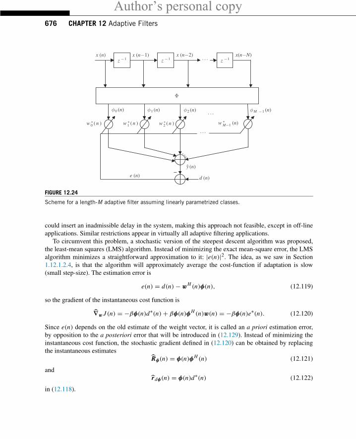
Author’s personal copy676 CHAPTER 12 Adaptive Filters
z −1z −1z −1
. . .
. . .
. . .x (n) x (n−1) x (n−2) x(n−N)
Φ
w ∗0 ( n ) w ∗
1 ( n ) w ∗2 ( n ) w ∗
M−1 (n)
φ0 (n) φ1 (n) φ2 (n) φM −1 (n)
y (n)
d (n)e (n)
FIGURE 12.24
Scheme for a length-M adaptive filter assuming linearly parametrized classes.
could insert an inadmissible delay in the system, making this approach not feasible, except in off-lineapplications. Similar restrictions appear in virtually all adaptive filtering applications.
To circumvent this problem, a stochastic version of the steepest descent algorithm was proposed,the least-mean squares (LMS) algorithm. Instead of minimizing the exact mean-square error, the LMSalgorithm minimizes a straightforward approximation to it: |e(n)|2. The idea, as we saw in Section1.12.1.2.4, is that the algorithm will approximately average the cost-function if adaptation is slow(small step-size). The estimation error is
e(n) = d(n)− wH (n)φ(n), (12.119)
so the gradient of the instantaneous cost function is
∇w J (n) = −βφ(n)d∗(n)+ βφ(n)φH (n)w(n) = −βφ(n)e∗(n). (12.120)
Since e(n) depends on the old estimate of the weight vector, it is called an a priori estimation error,by opposition to the a posteriori error that will be introduced in (12.129). Instead of minimizing theinstantaneous cost function, the stochastic gradient defined in (12.120) can be obtained by replacingthe instantaneous estimates
Rφ(n) = φ(n)φH (n) (12.121)
andrdφ(n) = φ(n)d∗(n) (12.122)
in (12.118).
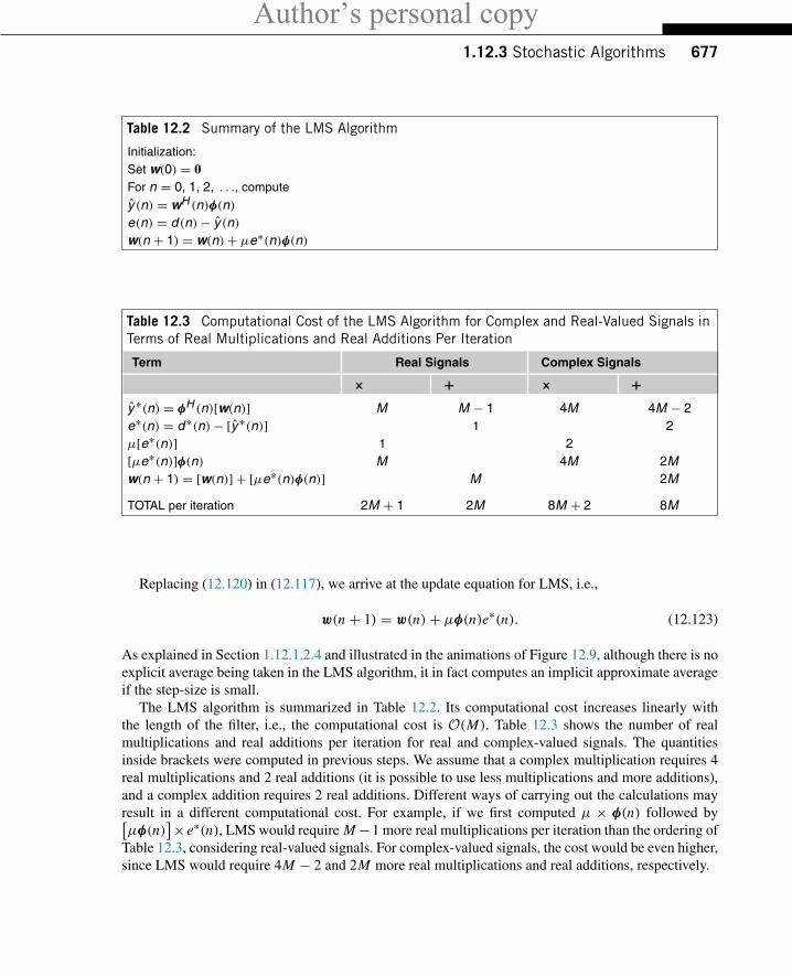
Author’s personal copy1.12.3 Stochastic Algorithms 677
Table 12.2 Summary of the LMS Algorithm
Initialization:Set w(0) = 0For n = 0, 1, 2, . . ., compute
y (n) = wH (n)φ(n)e(n) = d (n)− y (n)w(n + 1) = w(n)+ μe∗(n)φ(n)
Table 12.3 Computational Cost of the LMS Algorithm for Complex and Real-Valued Signals inTerms of Real Multiplications and Real Additions Per Iteration
Term Real Signals Complex Signals
× + × +y ∗(n) = φH (n)[w(n)] M M − 1 4M 4M − 2e∗(n) = d∗(n)− [y ∗(n)] 1 2μ[e∗(n)] 1 2[μe∗(n)]φ(n) M 4M 2Mw(n + 1) = [w(n)] + [μe∗(n)φ(n)] M 2M
TOTAL per iteration 2M + 1 2M 8M + 2 8M
Replacing (12.120) in (12.117), we arrive at the update equation for LMS, i.e.,
w(n + 1) = w(n)+ μφ(n)e∗(n). (12.123)
As explained in Section 1.12.1.2.4 and illustrated in the animations of Figure 12.9, although there is noexplicit average being taken in the LMS algorithm, it in fact computes an implicit approximate averageif the step-size is small.
The LMS algorithm is summarized in Table 12.2. Its computational cost increases linearly withthe length of the filter, i.e., the computational cost is O(M). Table 12.3 shows the number of realmultiplications and real additions per iteration for real and complex-valued signals. The quantitiesinside brackets were computed in previous steps. We assume that a complex multiplication requires 4real multiplications and 2 real additions (it is possible to use less multiplications and more additions),and a complex addition requires 2 real additions. Different ways of carrying out the calculations mayresult in a different computational cost. For example, if we first computed μ × φ(n) followed by[μφ(n)
]×e∗(n), LMS would require M−1 more real multiplications per iteration than the ordering ofTable 12.3, considering real-valued signals. For complex-valued signals, the cost would be even higher,since LMS would require 4M − 2 and 2M more real multiplications and real additions, respectively.
Author’s personal copy678 CHAPTER 12 Adaptive Filters
1.12.3.1.1 A deterministic approach for the stability of LMSFinding the range of step-sizes such that the recursion (12.123) converges is a complicated task. Thereare two main approaches to finding the maximum step-size: an average approach and a deterministic(worst-case) approach. The average approach will be treated in Section 1.12.4.3. Since the deterministicapproach is easy to explain intuitively, we address it in the sequel (although a precise proof is not sosimple, see [35,36] for a full analysis).
For simplicity, assume that our filter is such that d(n) ≡ 0. Although this is not a very likely situationto encounter in practice, it allows us to avoid technical details that would complicate considerably thediscussion, and still arrive at the important conclusions.
Let us rewrite the LMS recursion, expanding the error with d(n) = 0 as e∗(n) = −(wH (n)φ(n))∗ =−φH (n)w(n) to obtain
w(n + 1) =[
I − μφ(n)φH (n)]w(n). (12.124)
This is a linear system, but not a time-invariant one. It will be stable if the eigenvalues λi (n) of thematrix A(n) = I − μφ(n)φH (n) satisfy
maxi|λi (n)| ≤ 1, for all n ≥ 0. (12.125)
Be careful, if d(n) were not identically zero, condition (12.125) would have to be slightly modified toguarantee stability (see, e.g., [36,37]).
The eigenvalues of A(n) are easy to find, if we note that φ(n) is an eigenvector of A(n) (the caseφ(n) = 0 is trivial):
A(n)φ(n) = φ(n)− μφ(n)φH (n)φ(n) = (1− μ‖φ(n)‖2)φ(n),where ‖φ(n)‖2 = φH (n)φ(n) is the square of the Euclidean norm. The corresponding eigenvalue isλ1 = 1−μ‖φ(n)‖2. All other eigenvalues are equal to one (the eigenvectors are all vectors orthogonalto φ(n).) Therefore, the LMS algorithm (12.124) will be stable whenever
− 1 ≤ 1− μ‖φ(n)‖2 ≤ 1⇐⇒ 0 ≤ μ ≤ 2
supn≥0 ‖φ(n)‖2. (12.126)
The supremum (sup) of a sequence is an extension to the maximum, defined to avoid a technicality.Consider the sequence f (n) = {1− 0.5n}, n ≥ 0. Strictly speaking, it has no maximum, since there isno n0 for which f (n0) ≥ f (n) for all n ≥ 0. The supremum is defined so we can avoid this problem:supn≥0 f (n) = 1. Therefore, the supremum is equal to the maximum whenever the later exists, but isalso defined for some sequences that do not have a maximum. The infimum ( inf ) has a similar relationto the minimum.
This condition is sufficient for stability, but is too conservative, since ‖φ(n)‖2 is not at its highestvalue at all instants. A popular solution is to use normalization. The idea is simple: adopt a time-variantstep-size μ(n) such that
μ(n) = μ
ε + ‖φ(n)‖2 , (12.127)
with 0 < μ < 2 and where ε > 0 is used to avoid division by zero. The resulting algorithm is knownas normalized LMS (NLMS). We will talk more about it in the next section.
Author’s personal copy1.12.3 Stochastic Algorithms 679
1.12.3.2 Normalized LMS algorithmOne problem with the LMS algorithm is how to choose the step-size. How large should it be to enable ahigh convergence rate, provide an acceptable misadjustment, and even ensure the stability of LMS? Moreimportantly, how can this choice be made so that the filter will work correctly even for very differentinput signals? One answer to this problem is the normalized LMS algorithm which we describe now. Ituses a time varying step-size, which is particularly useful when the statistics of the input signals changequickly.
Thus, replacing the fixed step-size μ by a time varying step-size μ(n) in (12.123), we obtain
w(n + 1) = w(n)+ μ(n)φ(n)e∗(n). (12.128)
In order to increase the convergence speed, we could try to findμ(n) such that the a posteriori estimationerror,
ξ(n) = d(n)− wH (n + 1)φ(n), (12.129)
is zeroed. Note that, in contrast to the a priori estimation error defined in (12.119), ξ(n) depends on theupdated estimate of the weight vector, hence the name a posteriori estimation error. Replacing (12.128)in (12.129), we obtain
ξ(n) = d(n)− wH (n)φ(n)︸ ︷︷ ︸e(n)
−μ(n)φH (n)φ(n)e(n)
= [1− μ(n)φH (n)φ(n)]e(n). (12.130)
In order to enforce ξ(n) = 0 at each time instant n, we must select
μ(n) = 1
φH (n)φ(n)= 1
‖φ(n)‖2 . (12.131)
Replacing (12.131) in (12.128), we obtain the update equation of the normalized least-squares algo-rithm, i.e.,
w(n + 1) = w(n)+ 1
‖φ(n)‖2 φ(n)e∗(n). (12.132)
Note that the time varying step-size μ(n) depends inversely on the instantaneous power of the inputvector φ(n). Indeed, we will show in Section 1.12.4.3 that the maximum value of the fixed step-sizeμ to ensure the convergence and mean-square stability of LMS depends inversely on the power of theinput signal.
In order to make (12.132) more reliable for practical implementations, it is common to introducetwo positive constants: a fixed step-size μ to control the rate of convergence (and the misadjustment)and the regularization factor ε to prevent division by a small value when ‖φ(n)‖2 is small. With theseconstants, the NLMS update equation reduces to
w(n + 1) = w(n)+ μ
ε + ‖φ(n)‖2 φ(n)e∗(n). (12.133)
Author’s personal copy680 CHAPTER 12 Adaptive Filters
Some authors refer to (12.132) as NLMS and to (12.133) as ε-NLMS. However, for simplicity wewill refer to both as NLMS. The name “normalized” is due to a most useful property of NLMS: therange of values of μ for which the algorithm remains stable is independent of the statistics of x(n), i.e.,0 < μ < 2, as can be observed in Section 1.12.3.1.1.
As pointed out in [3], the NLMS algorithm can also be interpreted as a quasi-Newton algorithm. Asbriefly explained in Box 1, a quasi-Newton algorithm updates the weights using approximations for theHessian matrix and gradient vector, i.e.,
w(n + 1) = w(n)− μβ
[∇2
w J (n)]−1 ∇w J (n). (12.134)
Assuming the following instantaneous approximations
∇w J (n) = −βφ(n)d∗(n)+ βφ(n)φH (n)w(n) = −βφ(n)e∗(n) (12.135)
and∇2
w J (n) = ε I + φ(n)φH (n), (12.136)
and replacing them in (12.134), we arrive at the stochastic recursion
w(n + 1) = w(n)+ μ[ε I + φ(n)φH (n)
]−1φ(n)e∗(n). (12.137)
The term ε I guarantees that (12.136) is invertible (a rank-one matrix such as φ(n)φH (n) is neverinvertible).
To compute [ε I + φ(n)φH (n)]−1, we can use the matrix inversion lemma (Box 3), which gives usan expression for the inverse of an M × M matrix of the form
A = B + C DC H , (12.138)
where B and D are two square matrices with dimensions M and N , respectively, and C is an M × Nmatrix. According to the matrix inversion lemma, the inverse of A is given by
A−1 = B−1 − B−1C(D−1 + C H B−1C)−1C H B−1. (12.139)
Thus, identifying
A = ε I + φ(n)φH (n), B = ε I, C = φ(n), and D = 1,
we obtain
[ε I + φ(n)φH (n)]−1 = ε−1 I − ε−2
1+ ε−1φH (n)φ(n)φ(n)φH (n). (12.140)
Multiplying (12.140) from the right by φ(n), after some algebraic manipulations, we get
[ε I + φ(n)φH (n)]−1φ(n) = φ(n)
ε + φH (n)φ(n)= φ(n)
ε + ‖φ(n)‖2 . (12.141)
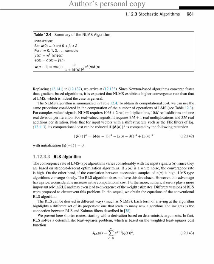
Author’s personal copy1.12.3 Stochastic Algorithms 681
Table 12.4 Summary of the NLMS Algorithm
Initialization:Set w(0) = 0 and 0 < μ < 2For n = 0, 1, 2, . . ., compute
y (n) = wH (n)φ(n)e(n) = d (n)− y (n)
w(n + 1) = w(n)+ μ
ε + ‖φ(n)‖2 e∗(n)φ(n)
Replacing (12.141) in (12.137), we arrive at (12.133). Since Newton-based algorithms converge fasterthan gradient-based algorithms, it is expected that NLMS exhibits a higher convergence rate than thatof LMS, which is indeed the case in general.
The NLMS algorithm is summarized in Table 12.4. To obtain its computational cost, we can use thesame procedure considered in the computation of the number of operations of LMS (see Table 12.3).For complex-valued signals, NLMS requires 10M + 2 real multiplications, 10M real additions and onereal division per iteration. For real-valued signals, it requires 3M + 1 real multiplications and 3M realadditions per iteration. Note that for input vectors with a shift structure such as the FIR filters of Eq.(12.113), its computational cost can be reduced if ‖φ(n)‖2 is computed by the following recursion
‖φ(n)‖2 = ‖φ(n − 1)‖2 − |x(n − M)|2 + |x(n)|2 (12.142)
with initialization ‖φ(−1)‖ = 0.
1.12.3.3 RLS algorithmThe convergence rate of LMS-type algorithms varies considerably with the input signal x(n), since theyare based on steepest-descent optimization algorithms. If x(n) is a white noise, the convergence rateis high. On the other hand, if the correlation between successive samples of x(n) is high, LMS-typealgorithms converge slowly. The RLS algorithm does not have this drawback. However, this advantagehas a price: a considerable increase in the computational cost. Furthermore, numerical errors play a moreimportant role in RLS and may even lead to divergence of the weight estimates. Different versions of RLSwere proposed to circumvent this problem. In the sequel, we obtain the equations of the conventionalRLS algorithm.
The RLS can be derived in different ways (much as NLMS). Each form of arriving at the algorithmhighlights a different set of its properties: one that leads to many new algorithms and insights is theconnection between RLS and Kalman filters described in [38].
We present here shorter routes, starting with a derivation based on deterministic arguments. In fact,RLS solves a deterministic least-squares problem, which is based on the weighted least-squares costfunction
JLS(n) =n∑�=0
λn−�|ξ(�)|2, (12.143)
Author’s personal copy682 CHAPTER 12 Adaptive Filters
where 0� λ < 1 is a constant known as forgetting factor,
ξ(�) = d(�)− wH φ(�), (12.144)
are a posteriori errors andw(n + 1) = arg min
wJLS(n). (12.145)
The factor λn−� emphasizes the most recent errors, forgetting the errors from the remote past. This isimportant, otherwise the algorithm would give too much weight to the remote past and would not beable to track variations in the input signals. Note that w(n + 1) minimizes JLS(n) at each time instant.Thus, RLS provides an exact solution for the least-squares problem at each time instant. As the NLMSalgorithm, RLS seeks to minimize the a posteriori error |ξ(n)|2, searching for an exact solution to anoptimization problem. The difference is that RLS searches for a weight vector w(n + 1) that takes intoconsideration the whole past history of inputs, minimizing λn|ξ(0)|2 + λn−1|ξ(1)|2 + · · · + λ|ξ(n −1)|2 + |ξ(n)|2 at each time instant n, not only the current value |ξ(n)|2 as in NLMS.
The error sequence ξ(�) weighted by λ(n−�)/2 in the interval 0 ≤ � ≤ n can be written in a vectorialform, i.e.,
ξ(n) = d(n)−�(n)w∗, (12.146)
where
ξ(n) = [ξ(n) λ1/2ξ(n − 1) · · · λn/2ξ(0)
]T, (12.147)
d(n) = [d(n) λ1/2d(n − 1) · · · λn/2d(0)
]T(12.148)
and
�(n) =
⎡⎢⎢⎢⎢⎢⎣φ0(n) φ1(n) · · · φM−1(n)
λ1/2φ0(n − 1) λ1/2φ1(n − 1) · · · λ1/2φM−1(n − 1)λφ0(n − 2) λφ1(n − 2) · · · λφM−1(n − 2)
.... . .
. . ....
λn/2φ0(0) λn/2φ1(0) · · · λn/2φM−1(0)
⎤⎥⎥⎥⎥⎥⎦ . (12.149)
Note that the weighted least-squares cost function can be rewritten in terms of the vector ξ(n), i.e.,
JLS(n) = ξ H (n)ξ(n) = ‖ξ(n)‖2 =n∑�=0
λn−�|ξ(�)|2. (12.150)
Now, we have to find the weight vector w(n + 1) that minimizes (12.150). The gradient of JLS(n)with relation to wH is given by
∇w JLS(n) = −β�T (n)d∗(n)+ β�T (n)�∗(n)w, (12.151)
where as usual, β = 1 (resp., β = 2) for complex (resp., real) data. Defining
Rφ(n) = �T (n)�∗(n) =n∑�=0
λn−�φ(�)φH (�) (12.152)
Author’s personal copy1.12.3 Stochastic Algorithms 683
and
rdφ(n) = �T (n)d∗(n) =n∑�=0
λn−�d∗(�)φ(�), (12.153)
in which φ(n) is defined as before, (12.151) can be rewritten as
∇w JLS(n) = −β rdφ(n)+ β Rφ(n)w. (12.154)
Equating ∇w JLS(n) to the null vector, we get the normal equations
Rφ(n)w(n + 1) = rdφ(n). (12.155)
Note that these are a deterministic version of the normal equations we saw in Section 1.12.2.1. Therefore,to minimize JLS(n), the weight vector w(n + 1) must satisfy
w(n + 1) = R−1φ (n)rdφ(n), (12.156)
which requires the computation of the inverse correlation matrix R−1φ (n) at each time instant. Note that
this is only valid if R−1φ (n) is nonsingular. In particular, the inverse does not exist if n < M (Box 3).
Assuming λ = 1 and that the signals x(n) and d(n) are jointly stationary and ergodic, we obtain thefollowing steady-state relations
limn→∞
1
n + 1Rφ(n)|λ=1 = Rφ and lim
n→∞1
n + 1rdφ(n)|λ=1 = rdφ .
Therefore, the deterministic normal equations converge to the stochastic normal equations when λ = 1,and the weight vector obtained from (12.156) converges to the Wiener solution, i.e.,
limn→∞w(n + 1)|λ=1 = R−1
φ rdφ = wo. (12.157)
We should mention that with λ = 1 the convergence rate of RLS goes to zero, i.e., it loses the ability tofollow the statistical variations of the observed data. An equivalent result is obtained for LMS or NLMSwhen the fixed step-size μ or μ is replaced by 1/n [39].
The computational cost of (12.156) is high due to the computation of the inverse matrix. In order tosolve the normal equations in real-time and with less cost, we should rewrite (12.152) and (12.153) asrecursions, i.e.,
Rφ(n) = λRφ(n − 1)+ φ(n)φH (n), (12.158)
andrdφ(n) = λrdφ(n − 1)+ d∗(n)φ(n), (12.159)
with initializations Rφ(−1) = δ I and rdφ(−1) = 0, where δ is a small positive constant. Note that(12.159) is identical to (12.153), but (12.158) leads to the estimate
Rφ(n) = λn+1δ I +n∑�=0
λn−�φ(�)φH (�), (12.160)
Author’s personal copy684 CHAPTER 12 Adaptive Filters
and therefore the initialization guarantees the existence of the inverse at all instants. For 0 � λ < 1,the initialization Rφ(−1) = δ I is forgotten and (12.158) becomes close to (12.152) as n increases.Furthermore, if you want the algorithm to forget quickly the initialization, besides using 0 � λ < 1,you should choose δ small (δ−1 large). Note however that a certain amount of regularization may beuseful in practice, to avoid problems when the input signal has long stretches with low power.
In order to obtain a recursion for the inverse matrix R−1φ (n), we can use the matrix inversion lemma
(Box 3) by comparing (12.138) with (12.158) and identifying
A = Rφ(n), B = λRφ(n − 1), C = φ(n), and D = 1.
Thus, using (12.139), we obtain
R−1φ (n) = λ−1 R
−1φ (n − 1)− λ
−2 R−1φ (n − 1)φ(n)φH (n)R
−1φ (n − 1)
1+ λ−1φH (n)R−1φ (n − 1)φ(n)
. (12.161)
Defining P(n) � R−1φ (n), with some algebraic manipulations in (12.161), we arrive at
P(n) = 1
λ
[P(n − 1)− P(n − 1)φ(n)φH (n)P(n − 1)
λ+ φH P(n − 1)φ(n)
](12.162)
with initialization P(−1) = δ−1 I . This equation allow us to compute the inverse correlation matrix ina recurrent form, avoiding the explicit computation of a matrix inverse. However, the implementationof (12.162) in finite precision arithmetic requires some care to avoid numerical problems, as explainedin Section 1.12.3.3.1.
To simplify the following equations, it is convenient to define the column vector
k(n) = P(n − 1)φ(n)
λ+ φH (n)P(n − 1)φ(n), (12.163)
which is the so-called Kalman gain. Thus, (12.162) can be rewritten as
P(n) = λ−1[
I − k(n)φH (n)]
P(n − 1). (12.164)
Using (12.164) and some algebraic manipulations in (12.163), we arrive at
k(n) = λ−1 P(n − 1)φ(n)− λ−1k(n)φH (n)P(n − 1)φ(n)
= λ−1[
I − k(n)φH (n)]
P(n − 1)φ(n)
= P(n)φ(n). (12.165)
Thus, using (12.159) and (12.165) in (12.156), the weight vector w(n + 1) can also be computedrecursively, i.e.,
w(n + 1) = P(n)rdφ(n)
= λP(n)rdφ(n − 1)+ P(n)φ(n)d∗(n)= λP(n)rdφ(n − 1)+ k(n)d∗(n). (12.166)
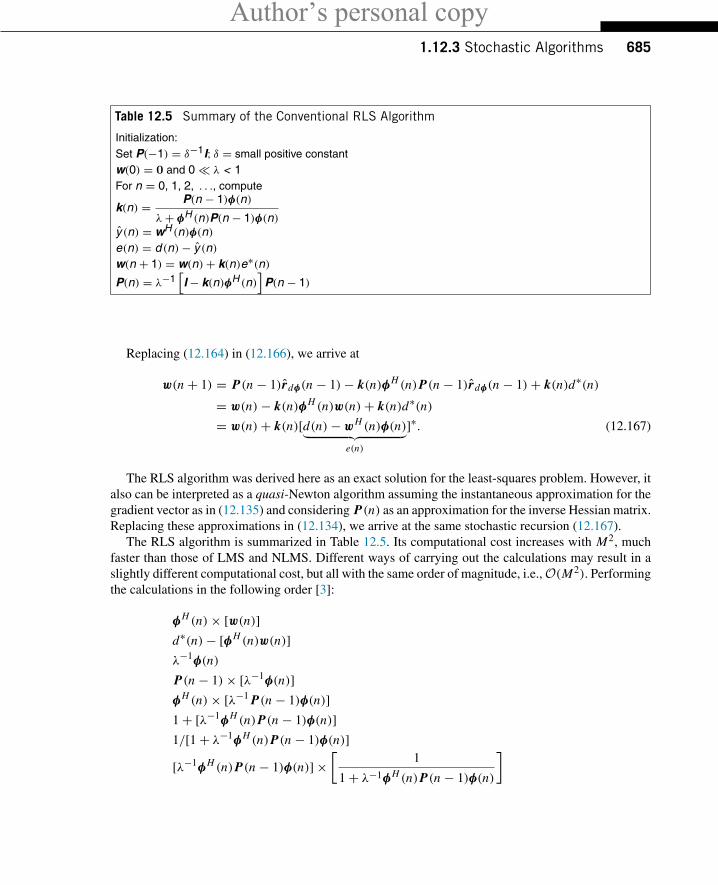
Author’s personal copy1.12.3 Stochastic Algorithms 685
Table 12.5 Summary of the Conventional RLS Algorithm
Initialization:Set P(−1) = δ−1I; δ = small positive constantw(0) = 0 and 0� λ < 1For n = 0, 1, 2, . . ., compute
k(n) = P(n − 1)φ(n)
λ+ φH (n)P(n − 1)φ(n)y (n) = wH (n)φ(n)e(n) = d (n)− y (n)w(n + 1) = w(n)+ k(n)e∗(n)P(n) = λ−1
[I− k(n)φH (n)
]P(n − 1)
Replacing (12.164) in (12.166), we arrive at
w(n + 1) = P(n − 1)rdφ(n − 1)− k(n)φH (n)P(n − 1)rdφ(n − 1)+ k(n)d∗(n)= w(n)− k(n)φH (n)w(n)+ k(n)d∗(n)= w(n)+ k(n)[d(n)− wH (n)φ(n)︸ ︷︷ ︸
e(n)
]∗. (12.167)
The RLS algorithm was derived here as an exact solution for the least-squares problem. However, italso can be interpreted as a quasi-Newton algorithm assuming the instantaneous approximation for thegradient vector as in (12.135) and considering P(n) as an approximation for the inverse Hessian matrix.Replacing these approximations in (12.134), we arrive at the same stochastic recursion (12.167).
The RLS algorithm is summarized in Table 12.5. Its computational cost increases with M2, muchfaster than those of LMS and NLMS. Different ways of carrying out the calculations may result in aslightly different computational cost, but all with the same order of magnitude, i.e., O(M2). Performingthe calculations in the following order [3]:
φH (n)× [w(n)]d∗(n)− [φH (n)w(n)]λ−1φ(n)
P(n − 1)× [λ−1φ(n)]φH (n)× [λ−1 P(n − 1)φ(n)]1+ [λ−1φH (n)P(n − 1)φ(n)]1/[1+ λ−1φH (n)P(n − 1)φ(n)][λ−1φH (n)P(n − 1)φ(n)] ×
[1
1+ λ−1φH (n)P(n − 1)φ(n)
]
Author’s personal copy686 CHAPTER 12 Adaptive Filters
[λ−1 P(n − 1)φ(n)] ×[
λ−1φH (n)P(n − 1)φ(n)
1+ λ−1φH (n)P(n − 1)φ(n)
]
P(n)φ(n) = [λ−1 P(n − 1)φ(n)] −[λ−2 P(n − 1)φ(n)φH (n)P(n − 1)φ(n)
1+ λ−1φH (n)P(n − 1)φ(n)
][P(n)φ(n)] × [d∗(n)− φH (n)w(n)]w(n + 1) = [w(n)] + [P(n)φ(n)(d∗(n)− φH (n)w(n))],
the conventional RLS requires 4M2+16M+1 real multiplications, 4M2+12M−1 real additions, andone real division per iteration for complex-valued signals. For real-valued data, it requires M2+5M+1real multiplications, M2+3M real additions, and one real division per iteration. Note that the quantitiesinside brackets were computed in previous steps.
1.12.3.3.1 Practical implementation of RLSThe RLS algorithm must be implemented carefully, because it is sensitive to numerical errors, whichmay accumulate and make the algorithm unstable. The problem can be understood intuitively as follows.In the conventional RLS algorithm, the inverse of the autocorrelation matrix is computed recursivelyby (expanding (12.161))
P(n) = λ−1 P(n − 1)− λ−2 P(n − 1)φ(n)φH (n)P(n − 1)
1+ λ−1φH (n)P(n − 1)φ(n),
i.e., as the difference between two positive (semi-) definite matrices. Note that, since λ ≤ 1, the factormultiplying the current P(n − 1) is λ−1 ≥ 1. In infinite precision arithmetic, any growth due to thisfactor will be compensated by the second term. However, in finite precision arithmetic this compensationmay not take place, and the factor λ−1 may make the recursion numerically unstable—usually, whathappens is that P(n) looses its positive character, so the matrix will have a negative eigenvalue, which inits turn leads to the divergence of the coefficients. Thus, to avoid problems one would need to guaranteethat P(n) stays symmetric and positive-definite for all time instants n (these properties are known asbackward consistency of RLS [40,41]). Symmetry can be guaranteed by computing only the upper orlower triangular part of P(n), and copying the result to obtain the rest of elements. However, it is alsonecessary to guarantee positive-definiteness. Reference [42] describes how this can be achieved.
Due to the fast convergence rate of RLS, a large literature is devoted to finding numerically stable andlow-cost (i.e., O(M)) versions of RLS. This is not an easy problem, that required the work of numerousresearchers to be solved. Nowadays the user has a very large number of different versions of RLS tochoose from. There are versions with formal proofs of stability, versions that work well in practice,but without formal proofs, versions with O(M2) complexity, and versions with O(M) complexity. Theinterested reader can find more references in Section 1.12.5.1.2.
One approach to ensure the consistency of P(n) uses a property of symmetric and positive-definitematrices (see Box 3): Cholesky factorizations. A symmetric and positive-definite matrix P(n) may
Author’s personal copy1.12.3 Stochastic Algorithms 687
always be factored asP(n) = P(n)P H (n), (12.168)
where P(n) is a lower triangular M×M matrix, called Cholesky factor of P(n). Thus, an algorithm thatcomputes P(n) instead of P(n) can avoid the numerical instability of the conventional RLS algorithm.There are many algorithms based on this main idea; for some of them a precise stability proof is available[40]. A recent and very complete survey of QR-RLS algorithms is available in [43].
Another approach is available when the regressor sequence {φ(n)} has shift structure. In this case,it is possible to derive lattice-based RLS filters that are in practice stable, although no formal proof isavailable at this time, as described, for example, in [5].
A more practical solution for the implementation of the RLS algorithm was proposed recently in[44]. This approach avoids propagation of the inverse covariance matrix, using an iterative method tosolve (12.155) at each step. The computational complexity is kept low by using the previous solutionas initialization, and by restricting the majority of the multiplications to multiplications by powers oftwo (which can be implemented as simple shifts). See Section 1.12.5.1.3.
1.12.3.4 Comparing convergence ratesTo compare the convergence of LMS, NLMS, and RLS, we show next two examples. In Example 1, weconsider a system identification application and in Example 2, we use these algorithms to update theweights of an equalizer.
As we will see in more detail in Section 1.12.4, adaptive filters are compared based on how well theyhandle different classes of signals. For example, we could be interested in seeing how two filters handlewhite noise, or how they handle a certain level of correlation at the input. Given the stochastic nature ofthe inputs, the performance measures are defined in terms of averaged cost functions, most commonlythe mean-square error (MSE), that is, the average of |e(n)|2 over all possible inputs in a given class.These averages can be computed theoretically, as we show in Section 1.12.4, or via simulations.
For example, the MSE as a function of time, that is, the curve E{|e(n)|2} × n, is called a filter’slearning curve. A comparison of learning curves obtained theoretically and from simulations can beseen in Figure 12.30 further ahead. When simulations are used, one runs a filter L times for an intervalof N samples, starting always from the same conditions. For each run �, the error e(�)(n) is computedfor 1 ≤ n ≤ N , and one obtains the so-called ensemble-average learning curve
E(n)�= 1
L
L∑�=1
|e(�)(n)|2.
Usually the ensemble-average learning curve will be a reasonable approximation of the true learningcurve for a reasonably small value of L (say, from 50 to 1000), but in some situations this may not betrue—see [45,46] for examples and a detailed explanation.
Example 1. The aim of this example is to identify the system wo = [1 − 0.8]T , assuming that theregressor φ(n) is obtained from a process x(n) generated with a first-order autoregressive model, whosetransfer function is 1/(1 − 0.8z−1). This model is fed with an i.i.d. Gaussian random process withunitary variance. Moreover, additive i.i.d. noise v(n) with variance σ 2
v = 0.01 is added to form thedesired signal.
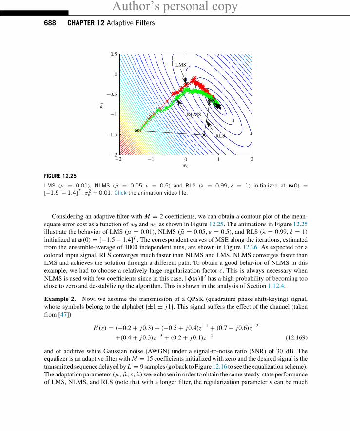
Author’s personal copy688 CHAPTER 12 Adaptive Filters
0
0
0.5
21
−0.5
−1.5
−1
−1−2
−2w0
w1
NLMS
LMS
RLS
FIGURE 12.25
LMS (μ = 0.01), NLMS (μ = 0.05, ε = 0.5) and RLS (λ = 0.99, δ = 1) initialized at w(0) =[−1.5 − 1.4]T , σ2
v = 0.01. Click the animation video file.
Considering an adaptive filter with M = 2 coefficients, we can obtain a contour plot of the mean-square error cost as a function of w0 and w1 as shown in Figure 12.25. The animations in Figure 12.25illustrate the behavior of LMS (μ = 0.01), NLMS (μ = 0.05, ε = 0.5), and RLS (λ = 0.99, δ = 1)initialized at w(0) = [−1.5− 1.4]T . The correspondent curves of MSE along the iterations, estimatedfrom the ensemble-average of 1000 independent runs, are shown in Figure 12.26. As expected for acolored input signal, RLS converges much faster than NLMS and LMS. NLMS converges faster thanLMS and achieves the solution through a different path. To obtain a good behavior of NLMS in thisexample, we had to choose a relatively large regularization factor ε. This is always necessary whenNLMS is used with few coefficients since in this case, ‖φ(n)‖2 has a high probability of becoming tooclose to zero and de-stabilizing the algorithm. This is shown in the analysis of Section 1.12.4.
Example 2. Now, we assume the transmission of a QPSK (quadrature phase shift-keying) signal,whose symbols belong to the alphabet {±1 ± j1}. This signal suffers the effect of the channel (takenfrom [47])
H(z) = (−0.2+ j0.3)+ (−0.5+ j0.4)z−1 + (0.7− j0.6)z−2
+(0.4+ j0.3)z−3 + (0.2+ j0.1)z−4 (12.169)
and of additive white Gaussian noise (AWGN) under a signal-to-noise ratio (SNR) of 30 dB. Theequalizer is an adaptive filter with M = 15 coefficients initialized with zero and the desired signal is thetransmitted sequence delayed by L = 9 samples (go back to Figure 12.16 to see the equalization scheme).The adaptation parameters (μ, μ, ε, λ)were chosen in order to obtain the same steady-state performanceof LMS, NLMS, and RLS (note that with a longer filter, the regularization parameter ε can be much
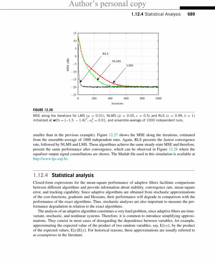
Author’s personal copy1.12.4 Statistical Analysis 689
0
0 200 400 600 800 1000−25
−20
−15
−10
−5
15
10
5
MSE
(dB
)LMS
NLMS
RLS
iterations
FIGURE 12.26
MSE along the iterations for LMS (μ = 0.01), NLMS (μ = 0.05, ε = 0.5) and RLS (λ = 0.99, δ = 1)initialized at w(0) = [−1.5 − 1.4]T , σ2
v = 0.01, and ensemble-average of 1000 independent runs.
smaller than in the previous example). Figure 12.27 shows the MSE along the iterations, estimatedfrom the ensemble-average of 1000 independent runs. Again, RLS presents the fastest convergencerate, followed by NLMS and LMS. These algorithms achieve the same steady-state MSE and therefore,present the same performance after convergence, which can be observed in Figure 12.28 where theequalizer output signal constellations are shown. The Matlab file used in this simulation is available athttp://www.lps.usp.br.
1.12.4 Statistical analysisClosed-form expressions for the mean-square performance of adaptive filters facilitate comparisonsbetween different algorithms and provide information about stability, convergence rate, mean-squareerror, and tracking capability. Since adaptive algorithms are obtained from stochastic approximationsof the cost-functions, gradients and Hessians, their performance will degrade in comparison with theperformance of the exact algorithms. Thus, stochastic analyses are also important to measure the per-formance degradation in relation to the exact algorithms.
The analysis of an adaptive algorithm constitutes a very hard problem, since adaptive filters are time-variant, stochastic, and nonlinear systems. Therefore, it is common to introduce simplifying approxi-mations. They consist in most cases of disregarding the dependence between variables, for example,approximating the expected value of the product of two random variables, say, E{xy}, by the productof the expected values, E{x}E{y}. For historical reasons, these approximations are usually referred toas assumptions in the literature.
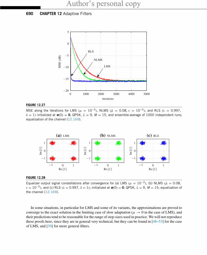
Author’s personal copy690 CHAPTER 12 Adaptive Filters
0
0 1000 2000 3000 4000 5000−20
−15
−10
−5
5
MSE
(dB
)
LMS
NLMS
RLS
iterations
FIGURE 12.27
MSE along the iterations for LMS (μ = 10−3), NLMS (μ = 0.08, ε = 10−5), and RLS (λ = 0.997,δ = 1) initialized at w(0) = 0; QPSK, L = 9, M = 15, and ensemble-average of 1000 independent runs;equalization of the channel (12.169).
0
0
−1
−1
1
1
(a) LMS
Im{y
}
Re{y}
0
0
−1
−1
1
1
(b) NLMS
Im{y
}
Re{y}
0
0
−1
−1
1
1
(c) RLS
Im{y
}
Re{y}
FIGURE 12.28
Equalizer output signal constellations after convergence for (a) LMS (μ = 10−3), (b) NLMS (μ = 0.08,ε = 10−5), and (c) RLS (λ = 0.997, δ = 1); initialized at w(0) = 0; QPSK, L = 9, M = 15; equalization ofthe channel (12.169).
In some situations, in particular for LMS and some of its variants, the approximations are proved toconverge to the exact solution in the limiting case of slow adaptation (μ→ 0 in the case of LMS), andtheir predictions tend to be reasonable for the range of step-sizes used in practice. We will not reproducethese proofs here, since they are in general very technical, but they can be found in [48–53] for the caseof LMS, and [39] for more general filters.
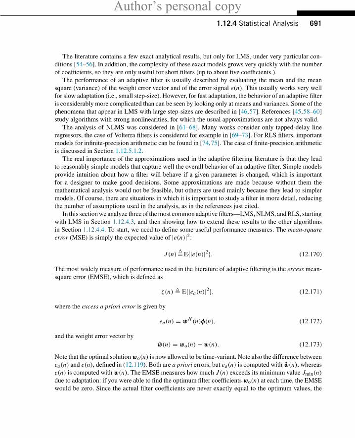
Author’s personal copy1.12.4 Statistical Analysis 691
The literature contains a few exact analytical results, but only for LMS, under very particular con-ditions [54–56]. In addition, the complexity of these exact models grows very quickly with the numberof coefficients, so they are only useful for short filters (up to about five coefficients.).
The performance of an adaptive filter is usually described by evaluating the mean and the meansquare (variance) of the weight error vector and of the error signal e(n). This usually works very wellfor slow adaptation (i.e., small step-size). However, for fast adaptation, the behavior of an adaptive filteris considerably more complicated than can be seen by looking only at means and variances. Some of thephenomena that appear in LMS with large step-sizes are described in [46,57]. References [45,58–60]study algorithms with strong nonlinearities, for which the usual approximations are not always valid.
The analysis of NLMS was considered in [61–68]. Many works consider only tapped-delay lineregressors, the case of Volterra filters is considered for example in [69–73]. For RLS filters, importantmodels for infinite-precision arithmetic can be found in [74,75]. The case of finite-precision arithmeticis discussed in Section 1.12.5.1.2.
The real importance of the approximations used in the adaptive filtering literature is that they leadto reasonably simple models that capture well the overall behavior of an adaptive filter. Simple modelsprovide intuition about how a filter will behave if a given parameter is changed, which is importantfor a designer to make good decisions. Some approximations are made because without them themathematical analysis would not be feasible, but others are used mainly because they lead to simplermodels. Of course, there are situations in which it is important to study a filter in more detail, reducingthe number of assumptions used in the analysis, as in the references just cited.
In this section we analyze three of the most common adaptive filters—LMS, NLMS, and RLS, startingwith LMS in Section 1.12.4.3, and then showing how to extend these results to the other algorithmsin Section 1.12.4.4. To start, we need to define some useful performance measures. The mean-squareerror (MSE) is simply the expected value of |e(n)|2:
J (n)�=E{|e(n)|2}. (12.170)
The most widely measure of performance used in the literature of adaptive filtering is the excess mean-square error (EMSE), which is defined as
ζ(n) � E{|ea(n)|2}, (12.171)
where the excess a priori error is given by
ea(n) = wH (n)φ(n), (12.172)
and the weight error vector byw(n) = wo(n)− w(n). (12.173)
Note that the optimal solution wo(n) is now allowed to be time-variant. Note also the difference betweenea(n) and e(n), defined in (12.119). Both are a priori errors, but ea(n) is computed with w(n), wherease(n) is computed with w(n). The EMSE measures how much J (n) exceeds its minimum value Jmin(n)due to adaptation: if you were able to find the optimum filter coefficients wo(n) at each time, the EMSEwould be zero. Since the actual filter coefficients are never exactly equal to the optimum values, the
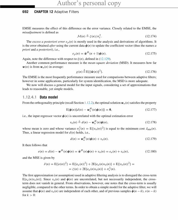
Author’s personal copy692 CHAPTER 12 Adaptive Filters
EMSE measures the effect of this difference on the error variance. Closely related to the EMSE, themisadjustment is defined as
M(n) � ζ(n)/σ 2v . (12.174)
The excess a posteriori error ep(n) is mostly used in the analysis and derivations of algorithms. Itis the error obtained after using the current data φ(n) to update the coefficient vector (thus the names apriori and a posteriori), i.e.,
ep(n) = wH (n + 1)φ(n). (12.175)
Again, note the difference with respect to ξ(n), defined in (12.129).Another common performance measure is the mean-square deviation (MSD). It measures how far
w(n) is from wo(n) in average:
χ(n)�=E{‖w(n)‖2}. (12.176)
The EMSE is the most frequently performance measure used for comparisons between adaptive filters;however in some applications, particularly for system identification, the MSD is more adequate.
We now will discuss a general model for the input signals, considering a set of approximations thatleads to reasonable, yet simple models.
1.12.4.1 Data modelFrom the orthogonality principle (recall Section 1.12.2), the optimal solution wo(n) satisfies the property
E{φ(n)[d(n)− wHo (n)φ(n)]} = 0, (12.177)
i.e., the input regressor vector φ(n) is uncorrelated with the optimal estimation error
vo(n) � d(n)− wHo (n)φ(n), (12.178)
whose mean is zero and whose variance σ 2v (n) = E{|vo(n)|2} is equal to the minimum cost Jmin(n).
Thus, a linear regression model for d(n) holds, i.e.,
d(n) = wHo (n)φ(n)+ vo(n). (12.179)
It then follows that
e(n) = d(n)− wH (n)φ(n) = wH (n)φ(n)+ vo(n) = ea(n)+ vo(n), (12.180)
and the MSE is given by
J (n) = E{|e(n)|2} = E{|ea(n)|2} + 2E{ea(n)vo(n)} + E{|vo(n)|2} == ζ(n)+ 2E{ea(n)vo(n)} + σ 2
v (n).
The first approximation (or assumption) used in adaptive filtering analysis is to disregard the cross-termE{ea(n)vo(n)}. Since vo(n) and φ(n) are uncorrelated, but not necessarily independent, the cross-term does not vanish in general. From observations, however, one notes that the cross-term is usuallynegligible, compared to the other terms. In order to obtain a simple model for the adaptive filter, we willassume that φ(n) and vo(n) are independent of each other, and of previous samples φ(n− k), v(n− k)for k > 0:
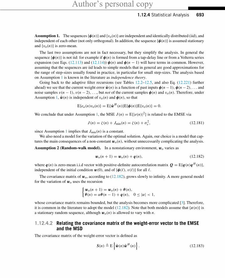
Author’s personal copy1.12.4 Statistical Analysis 693
Assumption 1. The sequences {φ(n)} and {vo(n)} are independent and identically distributed (iid), andindependent of each other (not only orthogonal). In addition, the sequence {φ(n)} is assumed stationaryand {vo(n)} is zero-mean.
The last two assumptions are not in fact necessary, but they simplify the analysis. In general thesequence {φ(n)} is not iid: for example if φ(n) is formed from a tap-delay line or from a Volterra seriesexpansion (see Eqs. (12.113) and (12.114)) φ(n) and φ(n − 1) will have terms in common. However,assuming that the sequences are iid leads to simple models that in general are good approximations forthe range of step-sizes usually found in practice, in particular for small step-sizes. The analysis basedon Assumption 1 is known in the literature as independence theory.
Going back to the adaptive filter recursions (see Tables 12.2–12.5, and also Eq. (12.221) furtherahead) we see that the current weight error w(n) is a function of past inputs φ(n− 1),φ(n− 2), . . . andnoise samples v(n − 1), v(n − 2), . . ., but not of the current samples φ(n) and vo(n). Therefore, underAssumption 1, w(n) is independent of vo(n) and φ(n), so that
E{ea(n)vo(n)} = E{wH (n)}E{φ(n)}E{vo(n)} = 0.
We conclude that under Assumption 1, the MSE J (n) = E{|e(n)|2} is related to the EMSE via
J (n) = ζ(n)+ Jmin(n) = ζ(n)+ σ 2v , (12.181)
since Assumption 1 implies that Jmin(n) is a constant.We also need a model for the variation of the optimal solution. Again, our choice is a model that cap-
tures the main consequences of a non-constant wo(n), without unnecessarily complicating the analysis.
Assumption 2 (Random-walk model). In a nonstationary environment, wo varies as
wo(n + 1) = wo(n)+ q(n), (12.182)
where q(n) is zero-mean i.i.d vector with positive-definite autocorrelation matrix Q = E{q(n)q H (n)},independent of the initial condition w(0), and of {φ(�), v(�)} for all �.
The covariance matrix of wo, according to (12.182), grows slowly to infinity. A more general modelfor the variation of wo uses the recursion{
wo(n + 1) = wo(n)+ θ(n),θ(n) = αθ(n − 1)+ q(n), 0 ≤ |α| < 1,
whose covariance matrix remains bounded, but the analysis becomes more complicated [3]. Therefore,it is common in the literature to adopt the model (12.182). Note that both models assume that {x(n)} isa stationary random sequence, although wo(n) is allowed to vary with n.
1.12.4.2 Relating the covariance matrix of the weight-error vector to the EMSEand the MSD
The covariance matrix of the weight-error vector is defined as
S(n) � E{w(n)wH (n)
}. (12.183)
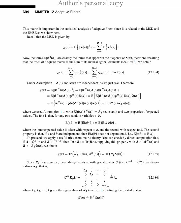
Author’s personal copy694 CHAPTER 12 Adaptive Filters
This matrix is important in the statistical analysis of adaptive filters since it is related to the MSD andthe EMSE as we show next.
Recall that the MSD is given by
χ(n) = E{‖w(n)‖2
}=
M−1∑i=0
E{w2
i (n)}.
Now, the terms E{w2i (n)} are exactly the terms that appear in the diagonal of S(n), therefore, recalling
that the trace of a square matrix is the sum of its main-diagonal elements (see Box 3), we obtain
χ(n) =M−1∑i=0
E{w2i (n)} =
M−1∑m=0
smm(n) = Tr(S(n)). (12.184)
Under Assumption 1, φ(n) and w(n) are independent, as we just saw. Therefore,
ζ(n) = E{|wH (n)φ(n)|2} = E{wH (n)φ(n)(wH (n)φ(n))∗}= E{wH (n)φ(n)φH (n)w(n)} = E
{E{wH (n)φ(n)φH (n)w(n)|w(n)}
}= E
{wH (n)E{φ(n)φH (n)|w(n)}w(n)
}= E{wH (n)Rφw(n)},
where we used Assumption 1 to write E{φ(n)φH (n)} = Rφ (constant), and two properties of expectedvalues. The first is that, for any two random variables a, b,
E{ab} = E {E{ab|b}} = E {E{a|b}b} ,where the inner expected value is taken with respect to a, and the second with respect to b. The secondproperty is that, if a and b are independent, then E{a|b} does not depend on b, i.e., E{a|b} = E{a}.
To proceed, we apply a useful trick from matrix theory. You can check by direct computation that,if A ∈ CK×L and B ∈ CL×K , then Tr(AB) = Tr(B A). Applying this property with A← wH (n) andB← Rφw(n), we obtain
ζ(n) = Tr(
RφE{w(n)wH (n)})= Tr
(Rφ S(n)
). (12.185)
Since Rφ is symmetric, there always exists an orthogonal matrix U (i.e., U−1 = U H ) that diago-nalizes Rφ , that is,
U H RφU =
⎡⎢⎢⎢⎣λ1 0 · · · 00 λ2 · · · 0...
.... . .
...
0 0 0 λM
⎤⎥⎥⎥⎦ �=�, (12.186)
where λ1, λ2, . . . , λM are the eigenvalues of Rφ (see Box 3). Defining the rotated matrix
S′(n) � U H S(n)U
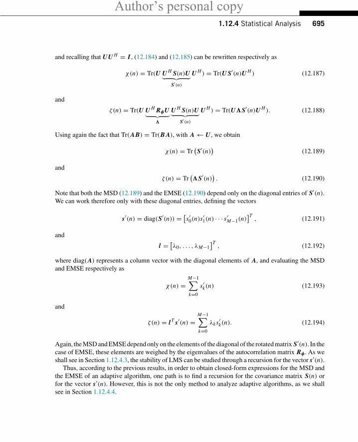
Author’s personal copy1.12.4 Statistical Analysis 695
and recalling that UU H = I , (12.184) and (12.185) can be rewritten respectively as
χ(n) = Tr(U U H S(n)U︸ ︷︷ ︸S′(n)
U H ) = Tr(U S′(n)U H ) (12.187)
and
ζ(n) = Tr(U U H RφU︸ ︷︷ ︸�
U H S(n)U︸ ︷︷ ︸S′(n)
U H ) = Tr(U�S′(n)U H ). (12.188)
Using again the fact that Tr(AB) = Tr(B A), with A← U , we obtain
χ(n) = Tr(S′(n)
)(12.189)
and
ζ(n) = Tr(�S′(n)
). (12.190)
Note that both the MSD (12.189) and the EMSE (12.190) depend only on the diagonal entries of S′(n).We can work therefore only with these diagonal entries, defining the vectors
s′(n) = diag(S′(n)) = [s′0(n)s′1(n) · · · s′M−1(n)
]T, (12.191)
and
l = [λ0, . . . , λM−1
]T, (12.192)
where diag(A) represents a column vector with the diagonal elements of A, and evaluating the MSDand EMSE respectively as
χ(n) =M−1∑k=0
s′k(n) (12.193)
and
ζ(n) = lT s′(n) =M−1∑k=0
λks′k(n). (12.194)
Again, the MSD and EMSE depend only on the elements of the diagonal of the rotated matrix S′(n). In thecase of EMSE, these elements are weighed by the eigenvalues of the autocorrelation matrix Rφ . As weshall see in Section 1.12.4.3, the stability of LMS can be studied through a recursion for the vector s′(n).
Thus, according to the previous results, in order to obtain closed-form expressions for the MSD andthe EMSE of an adaptive algorithm, one path is to find a recursion for the covariance matrix S(n) orfor the vector s′(n). However, this is not the only method to analyze adaptive algorithms, as we shallsee in Section 1.12.4.4.
Author’s personal copy696 CHAPTER 12 Adaptive Filters
1.12.4.3 Statistical analysis of the LMS algorithmIn this section, we present a statistical analysis for the LMS algorithm, assuming that the optimal solutionwo remains constant (q(n) ≡ 0, for all n). This analysis predicts the behavior of LMS in steady-stateand in transient, and provides a range of the step-size μ for which LMS operates adequately. If you arefamiliar with the LMS analysis, go to Section 1.12.4.4, where we present a unified analysis for LMS,NLMS, and RLS algorithms in a nonstationary environment.
We first rewrite (12.123) in terms of the weight-error vector w. Thus, subtracting both sides of(12.123) from wo, we obtain
wo − w(n + 1) = wo − w(n)− μφ(n)e∗(n),w(n + 1) = w(n)− μφ(n)e∗(n). (12.195)
Replacing e∗(n) = e∗a(n)+ v∗o(n) = φH (n)w(n)+ v∗o(n) in (12.195), we arrive at
w(n + 1) =[
I − μφ(n)φH (n)]w(n)− μφ(n)v∗o(n). (12.196)
First-order analysis. Taking expectations on both sides of (12.196), we obtain
E{w(n + 1)} = E{[
I − μφ(n)φH (n)]w(n)
}− μE{φ(n)v∗o(n)}
= E{[
I − μφ(n)φH (n)]w(n)
}, (12.197)
where the last equality follows from the fact that φ(n) is orthogonal to v∗o(n), according to the orthog-onality condition (see Eq. (12.96)). Since w(n) is assumed to be independent of φ(n) (see Assumption1), we arrive at
E{w(n + 1)} = [I − μRφ
]E{w(n)}. (12.198)
This is the same recursion we saw in Box 1. According to linear systems theory, this recursion convergesas long as the largest eigenvalue of A = I −μRφ has absolute value less than one, which implies (seeBox 1)
|1− μλ| < 1⇔ 0 < μ <2
λk, ∀k ⇔
0 < μ <2
λmax, (12.199)
where λk , k = 1, 2, . . . ,M are the eigenvalues of Rφ , and λmax is its maximum eigenvalue. We shouldnotice that this range for μ does not ensure the stability of LMS, since it ensures the convergence ofthe mean of w(n) = wo − w(n) towards 0, but the autocovariance of w(n) may still be diverging. Weshow next that the range for μ based on a second-order analysis is indeed more restrict.
Author’s personal copy1.12.4 Statistical Analysis 697
Second-order analysis. Now, we use (12.196) to find a recursion for S(n) and (12.185) to evaluate theEMSE of LMS. Multiplying (12.196) by its Hermitian, taking the expectations of both sides, we arrive at
E{w(n + 1)wH (n + 1)} = E{w(n)wH (n)}
−A︷ ︸︸ ︷
μE{w(n)wH (n)φ(n)φH (n)}
−B︷ ︸︸ ︷
μE{φ(n)φH (n)w(n)wH (n)}
+C︷ ︸︸ ︷
μ2E{φ(n)φH (n)w(n)wH (n)φ(n)φH (n)}
+D︷ ︸︸ ︷
μ2E{|vo(n)|2φ(n)φH (n)}
−E︷ ︸︸ ︷
μE{vo(n)w(n)φH (n)}
−F︷ ︸︸ ︷
μE{v∗o(n)φ(n)wH (n)}
+G︷ ︸︸ ︷
μ2E{vo(n)φ(n)φH (n)w(n)φH (n)}
+H︷ ︸︸ ︷
μ2E{v∗o(n)φ(n)wH (n)φ(n)φH (n)} . (12.200)
Now, using Assumption 1, we can evaluate the terms A−H of (12.200):
A- Recalling that Assumption 1 implies that w(n) is independent from φ(n), the term A can beapproximated by
A = μE{
E{w(n)wH (n)φ(n)φH (n)|φ(n)
}}≈ μE
{E{w(n)wH (n)
}φ(n)φH (n)
}= μS(n)E
{φ(n)φH (n)
}= μS(n)Rφ . (12.201)
B- Analogously, we obtain for BB ≈ μRφ S(n). (12.202)
C- Using Assumption 1, the term C can be rewritten as
C = μ2E{φ(n)φH (n)w(n)wH (n)φ(n)φH (n)
}≈ μ2E
{φ(n)φH (n)S(n)φ(n)φH (n)
}. (12.203)
We return to this term further on.
Author’s personal copy698 CHAPTER 12 Adaptive Filters
D- Using the fact that vo(n) is independent of φ(n) and w(n), D reduces to
D = μ2E{|vo(n)|2φ(n)φH (n)} ≈ μ2σ 2v Rφ . (12.204)
E- Using the fact that vo(n) is a zero-mean random variable, which is independent of φ(n) andw(n), E is a M × M null matrix. Using the same arguments, the terms F , G, and H are also nullmatrices. We should point out that the zero-mean assumption for vo(n) is not necessary, but it reallyfacilitates the analysis. Furthermore, as we saw in Section 1.12.2.1.4, we can enforce E{vo(n)} = 0using simple methods.
From the previous results, (12.200) reduces to
S(n + 1) ≈ S(n)− μS(n)Rφ − μRφ S(n)
+μ2E{φ(n)φH (n)S(n)φ(n)φH (n)
}︸ ︷︷ ︸
C
+μ2σ 2v Rφ . (12.205)
This recursion is convenient to obtain closed-form expressions for the EMSE and the MSD of LMS.Observe that the four first terms on the right-hand side of (12.205) are linear in S(n). Assuming that μis sufficiently small, the term C can be neglected with respect to the three first terms. Thus, for smallstep-sizes, (12.205) reduces to
S(n + 1) ≈ S(n)− μ [S(n)Rφ + Rφ S(n)]+ μ2σ 2
v Rφ, (12.206)
with initialization S(0) = [wo − w(0)
] [wo − w(0)
]H .Since we can obtain the EMSE and the MSD from S(n) and Rφ through (12.185) and (12.184), we
should use recursion (12.206) to compute S(n) and then, evaluate ζ(n) = Tr(S(n)Rφ) and χ(n) =Tr(S(n)). Particularly for n→∞, since S(n + 1) ≈ S(n), we obtain
S(∞)Rφ + Rφ S(∞) = μσ 2v Rφ . (12.207)
Taking the trace of both sides of (12.207), we arrive at an analytical expression for the steady-stateEMSE of LMS, i.e.,
ζLMS(∞) ≈ μσ 2v Tr(Rφ)
2(for sufficiently small μ). (12.208)
This expression indicates that the EMSE of LMS increases with μ and with the length of the filter. Thedependence with the filter length is through the trace of Rφ . It is more evident when the class of filters
we are considering is FIR, that is, when φ(n) = [x(n) . . . x(n − M + 1)
]T (a tapped-delay line). Inthis case, if {x(n)} is stationary, then Tr(Rφ) = ME{x2(n)}, M times the average power of x(n).
Turning now to the filter coefficients, if we multiply both sides of (12.207) from the right by R−1φ ,
taking the trace of both sides, and recalling that Tr(AB) = Tr(B A), we obtain an expression for thesteady-state MSD of LMS, i.e.,
χLMS(∞) ≈ μσ 2v M
2(for sufficiently small μ). (12.209)
Author’s personal copy1.12.4 Statistical Analysis 699
Again, the smaller the step-size μ and the filter length M , the smaller the MSD of LMS.These results explain what we observed in the simulations in Section 1.12.1.2 (Figures 12.9 and
12.10): for larger values of μ the filter converges faster, but hovers around the optimum solution in alarger region. The size of this region is what the MSD attempts to measure—the EMSE measures howmuch this hovering affects the error.
These quantities are important in practical situations. For example, in an actual implementation of anacoustic echo canceler, when the near-end user is speaking, his voice is part of v(n). Since the near-endspeech is normally stronger than the echo, σ 2
v tends to be quite large when the near-end speaker istalking. If the adaptive filter were allowed to keep adapting at these moments, (12.208) shows that thefilter estimates would wander too far from the optimum. To avoid this problem, the step-size is reducedto zero whenever the near-end user is speaking. A double-talk detector is used to decide when to stopadaptation.
It can be shown that (12.206) is stable for sufficiently small μ. However, (12.206) cannot be usedto find a range of values of μ that guarantee stability, due to the approximations made, particularly thediscarding of term C. Thus, in order to study the stability of LMS, we consider next an approximationfor this term, based the assumption that the input vector is Gaussian. This assumption allows us toapproximate C as
C ≈ RφTr(S(n)Rφ)+ βRφ S(n)Rφ, (12.210)
where as usual, β = 1 (resp., β = 2) for complex (resp., real) data. See Box 7 for the derivation of(12.210).
Replacing (12.210) in (12.205), we arrive at
S(n + 1) ≈ S(n)− μ [S(n)Rφ + Rφ S(n)]
+μ2[
RφTr(S(n)Rφ
)+ βRφ S(n)Rφ + σ 2v Rφ
]. (12.211)
The stability of (12.211) is determined through a recursion for the vector s′(n), which contains theelements of the diagonal of the rotated matrix S′(n) = U H S(n)U (see Section 1.12.4.2). A recursionfor S′(n) can be obtained by multiplying (12.211) from the left by U H and from the right by U andrecalling that UU H = I , which leads to
S′(n + 1) ≈ S′(n)− μ [S′(n)�+�S′(n)]
+μ2 [�Tr(�S′(n))+ β�S′(n)�]+ μ2σ 2
v�, (12.212)
where � is defined as in (12.186). Thus, a recursion for s′(n + 1) is given by
s′(n + 1) =[
I − 2μ�+ μ2(β�2 + l lT
)]s′(n)+ μ2σ 2
v l, (12.213)
where l is defined in (12.192).The system matrix A of (12.213) is given by
A = I − 2μ�+ μ2(β�2 + l lT
)= (
I − μ�)2 + μ2(β − 1)�2 + μ2l lT .
Author’s personal copy700 CHAPTER 12 Adaptive Filters
Although it is possible to obtain the exact values of all eigenvalues of A, as done in [36], we follow herea much simpler, approximate route. We can use Fact 7 in Box 3 to find an upper bound for the largesteigenvalue νi of A, using the 1-norm of A:
max0≤i≤M−1
|νi | ≤ ‖A‖1 = max0≤i≤M−1
M−1∑j = 0
|ai j |,
where ai j are the entries of A. If we find a range of μ for which ‖A‖1 ≤ 1, then the recursion will bestable. This will be of course a conservative condition (sufficient, but not necessary).
Now note that the ith column of A has entries λiλ j if i = j , and (1−μλi )2+μ2(β−1)λ2
i +μ2λ2i
in the term corresponding to the diagonal. Since all terms are positive, the 1-norm is
max0≤i≤M−1
⎡⎣(1− μλi )2 + μ2(β − 1)λ2
i + μ2λi
M−1∑j = 0
λ j
⎤⎦= max
0≤i≤M−1
[(1− μλi )
2 + μ2(β − 1)λ2i + μ2λi Tr(�)
].
Recall that Tr(�) = Tr(Rφ) (Fact 1 from Box 3). Therefore, the recursion will be stable if
1− 2μλi + μ2λ2i + μ2(β − 1)λ2
i + μ2λi Tr(Rφ) ≤ 1, 0 ≤ i ≤ M − 1.
Simplifying, we obtain the condition
μ ≤ 2
βλi + Tr(Rφ), 0 ≤ i ≤ M − 1.
The smallest bound is for λi = λmax:
μ ≤ 2
βλmax + Tr(Rφ). (12.214)
If we replace λmax by Tr(Rφ) ≥ λmax in the denominator, we obtain a simpler, but more conservativecondition:
μ ≤ 2
(β + 1)Tr(Rφ). (12.215)
For real data, this range reduces to
0 < μ <2
3Tr(Rφ)(real data) (12.216)
and for complex data to
0 < μ <1
Tr(Rφ)(complex data). (12.217)
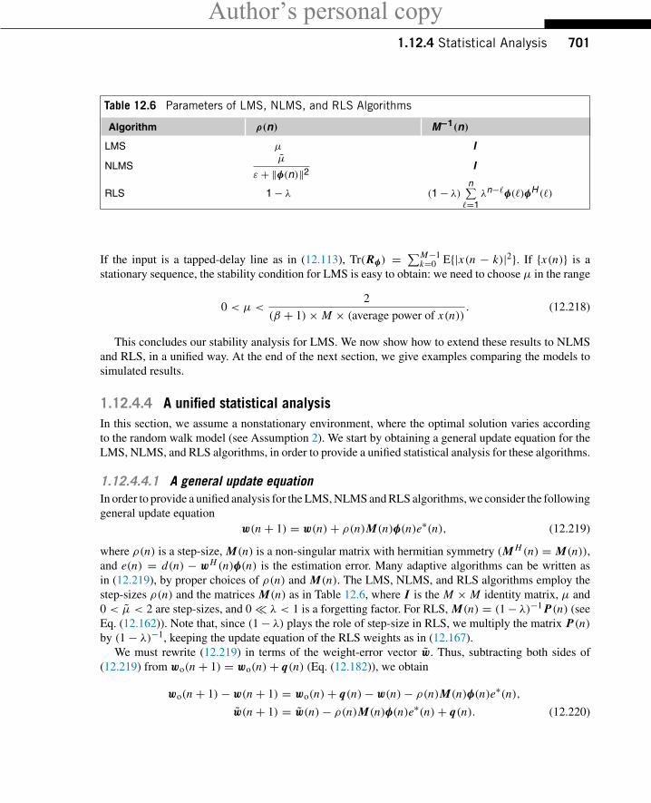
Author’s personal copy1.12.4 Statistical Analysis 701
Table 12.6 Parameters of LMS, NLMS, and RLS Algorithms
Algorithm ρ(n) M−1(n)
LMS μ I
NLMSμ
ε + ‖φ(n)‖2 I
RLS 1− λ (1− λ)n∑�=1
λn−�φ(�)φH (�)
If the input is a tapped-delay line as in (12.113), Tr(Rφ) = ∑M−1k=0 E{|x(n − k)|2}. If {x(n)} is a
stationary sequence, the stability condition for LMS is easy to obtain: we need to choose μ in the range
0 < μ <2
(β + 1)× M × (average power of x(n)). (12.218)
This concludes our stability analysis for LMS. We now show how to extend these results to NLMSand RLS, in a unified way. At the end of the next section, we give examples comparing the models tosimulated results.
1.12.4.4 A unified statistical analysisIn this section, we assume a nonstationary environment, where the optimal solution varies accordingto the random walk model (see Assumption 2). We start by obtaining a general update equation for theLMS, NLMS, and RLS algorithms, in order to provide a unified statistical analysis for these algorithms.
1.12.4.4.1 A general update equationIn order to provide a unified analysis for the LMS, NLMS and RLS algorithms, we consider the followinggeneral update equation
w(n + 1) = w(n)+ ρ(n)M(n)φ(n)e∗(n), (12.219)
where ρ(n) is a step-size, M(n) is a non-singular matrix with hermitian symmetry (M H (n) = M(n)),and e(n) = d(n) − wH (n)φ(n) is the estimation error. Many adaptive algorithms can be written asin (12.219), by proper choices of ρ(n) and M(n). The LMS, NLMS, and RLS algorithms employ thestep-sizes ρ(n) and the matrices M(n) as in Table 12.6, where I is the M × M identity matrix, μ and0 < μ < 2 are step-sizes, and 0� λ < 1 is a forgetting factor. For RLS, M(n) = (1− λ)−1 P(n) (seeEq. (12.162)). Note that, since (1− λ) plays the role of step-size in RLS, we multiply the matrix P(n)by (1− λ)−1, keeping the update equation of the RLS weights as in (12.167).
We must rewrite (12.219) in terms of the weight-error vector w. Thus, subtracting both sides of(12.219) from wo(n + 1) = wo(n)+ q(n) (Eq. (12.182)), we obtain
wo(n + 1)− w(n + 1) = wo(n)+ q(n)− w(n)− ρ(n)M(n)φ(n)e∗(n),w(n + 1) = w(n)− ρ(n)M(n)φ(n)e∗(n)+ q(n). (12.220)
Author’s personal copy702 CHAPTER 12 Adaptive Filters
Replacing e∗(n) = e∗a(n)+ v∗(n) = φH (n)w(n)+ v∗(n) in (12.220), we arrive at
w(n + 1) =[
I − ρ(n)M(n)φ(n)φH (n)]w(n)− ρ(n)M(n)φ(n)v∗(n)+ q(n). (12.221)
We next use recursion (12.221) to evaluate the EMSE and the MSD of LMS, NLMS, and RLS.
1.12.4.4.2 Alternative analysis methodsClosed-form expressions for the EMSE and MSD can be obtained in two ways:
i. Finding a recursion for the correlation matrix of the weight-error vector, denoted by S(n). TheEMSE and MSE can be easily computed given S(n), as we saw in Section 1.12.4.2. This is theearlier approach in the literature [1,2] and therefore, we refer to it here as traditional method.
ii. Using the energy conservation analysis of [3,76–78]. The energy conservation approach relieson an energy conservation relation that holds for a large class of adaptive filters. The energyconservation method presents some advantages when compared to the traditional one. For example,using energy conservation, one can obtain steady-state results directly, bypassing several of thedifficulties encountered in obtaining them as a limiting case of a transient analysis. This methodcan also be used in transient analyses of adaptive algorithms (see, e.g., Part V of [3]).
It is important to understand that both methods involve different sets of approximations (assumptions),so they do not always arrive at the same expressions. Generally, they tend to be equal in the limit of slowadaptation (i.e., if ρ(n) → 0 in (12.221)). For larger values of ρ(n), which method will provide thebest approximation depends on the algorithm. As for the work necessary to arrive at the final answers,the energy conservation approach is almost always easier to use if one is interested only in steady-stateresults. If one is interested in transient performance and stability studies, then the traditional methodmay be simpler, depending on the algorithm under study.
To give an overview of both methods, we first use the traditional method to obtain the transient andsteady-state performance of the LMS, NLMS, and RLS algorithms. This is an extension of what we didfor LMS in Section 1.12.4.3, taking advantage of the similarities between the algorithms. In the sequel,we employ the energy conservation method to obtain closed-form expressions for the steady-state EMSEof the same algorithms.
In this section we allow the environment to be nonstationary, i.e., the optimal solution wo is time-variant. The results for stationary environments can be obtained simply by making Q = 0 in theequations below. In order to simplify the arguments, we require that the regressor sequence {φ(n)} bewide-sense stationary, that is, we assume that Rφ is constant.
1.12.4.4.3 Analysis with the traditional methodThe traditional analysis method consists of finding a recursion for S(n), and using (12.184) and (12.185)to evaluate the MSD and the EMSE, respectively. A recursion for S(n) can be obtained by multiply-ing (12.221) by its Hermitian, taking the expectations of both sides, and recalling that Assumption 1implies that w(n) is independent of φ(n) and of the zero-mean vo(n). Furthermore, using the fact that
Author’s personal copy1.12.4 Statistical Analysis 703
E{w(n)q H (n)} = 0 since the sequence {q(n)} is iid (Assumption 2), we arrive at
E{w(n + 1)wH (n + 1)} = E{q(n)q H (n)} + E{w(n)wH (n)}
−A︷ ︸︸ ︷
E{ρ(n)w(n)wH (n)φ(n)φH (n)M(n)}
−B︷ ︸︸ ︷
E{ρ(n)M(n)φ(n)φH (n)w(n)wH (n)}
+C︷ ︸︸ ︷
E{ρ2(n)M(n)φ(n)φH (n)w(n)wH (n)φ(n)φH (n)M(n)}
+D︷ ︸︸ ︷
E{ρ2(n)|vo(n)|2 M(n)φ(n)φH (n)M(n)} . (12.222)
To simplify (12.222), we also need two additional assumptions:
Assumption 3. Matrix M(n) varies slowly in relation to w(n). Thus, when M(n) appears inside theexpectations of (12.222), we simply replace it by its mean. For LMS and NLMS, this assumption is notnecessary, since M(n) = I . For RLS, M(n) = (1− λ)−1 P(n) ≈ (1− λ)−1E{P(n)} if λ ≈ 1;
Assumption 4. The input regressor vector φ(n) is assumed to be Gaussian. This assumption makesthe analysis more tractable, since Gaussianity facilitates the computation of the expected values in C.
Now, using the Assumptions 1–4, we can evaluate the terms A-D of (12.222):
A- The term A can be approximated by
A = E{
E{ρ(n)w(n)wH (n)φ(n)φH (n)M(n)|φ(n)
}}≈ E
{ρ(n)E
{w(n)wH (n)
}φ(n)φH (n)
}E {M(n)}
= S(n)E{ρ(n)φ(n)φH (n)
}E {M(n)} . (12.223)
For LMS, this term reduces toALMS ≈ μS(n)Rφ . (12.224)
For NLMS, we must obtain an approximation for
E{ρ(n)φ(n)φH (n)
}= E
{μφ(n)φH (n)
ε + φH (n)φ(n)
}. (12.225)
It is possible to evaluate this expected value exactly (see [61,63,64]), but our intention here is toobtain the simplest possible model. Therefore, we will use two additional approximations:
Assumption 5. The number of coefficients M is large enough for each element φ(n)φH (n) in
the numerator to be approximately independent from the denominator∑M−1
k=0 |φ(n − k)|2.
Author’s personal copy704 CHAPTER 12 Adaptive Filters
This is equivalent to apply the averaging principle proposed in [79], since for large M, ‖φ(n)‖2 tendsto vary slowly compared to the individual entries of φ(n)φH (n).Thus, (12.225) can be approximated as
E
{φ(n)φH (n)
ε + φH (n)φ(n)
}≈ E
{1
ε + φH (n)φ(n)
}E{φ(n)φH (n)
}. (12.226)
Under Assumption 5, the first expected value in (12.226) can by approximated by:
E
{1
ε + φH (n)φ(n)
}≈ 1
E{ε + φH (n)φ(n)} =1
ε + Tr(Rφ). (12.227)
An alternative, more accurate approximation is obtained when φ(n) is Gaussian and a tapped-delayline:
Assumption 6. The regressor φ(n) is formed by a tapped-delay line with Gaussian entries as in(12.113), and ε = 0.
Under Assumptions 4, 5, and 6 it can be shown (see [65] for details) that
E
{1
ε + φH (n)φ(n)
}≈ 1
σ 2x (M − 2)
. (12.228)
Both approximations are only valid for long filters. However, (12.228) shows that NLMS needs alarge regularization constant if M < 3, which is verified in practice [63]. We will present the finalresults for NLMS in terms of Assumption 6, but recall that a less precise, but more general option isavailable using only Assumption 4 and approximations such as (12.227).Thus, the term A for NLMS reduces to (using (12.228))
ANLMS ≈ μ
σ 2x (M − 2)
S(n)Rφ . (12.229)
Finally, for RLS, we obtainARLS ≈ S(n)Rφ P(n), (12.230)
where P(n) � E{R−1φ (n)}, which we will evaluate later on.
B- Analogously, we obtain for B
B ≈ E {M(n)}E{ρ(n)φ(n)φH (n)
}S(n). (12.231)
Particularizing for each algorithm, we have
BLMS ≈ μRφ S(n), (12.232)
BNLMS ≈ μ
σ 2x (M − 2)
Rφ S(n), (12.233)
andBRLS ≈ P(n)Rφ S(n). (12.234)
Author’s personal copy1.12.4 Statistical Analysis 705
C- The term C can be approximated by
C = E{ρ2(n)M(n)φ(n)φH (n)w(n)wH (n)φ(n)φH (n)M(n)
}≈ E {M(n)}E
{ρ2(n)φ(n)φH (n)S(n)φ(n)φH (n)
}E {M(n)} . (12.235)
Under the Gaussianity assumption 4, it holds that (see Box 7)
E{φ(n)φH (n)S(n)φ(n)φH (n)
}= RφTr(S(n)Rφ)+ βRφ S(n)Rφ, (12.236)
where β = 1 (resp., β = 2) for complex (resp. real) data. Thus, for LMS we have
CLMS ≈ μ2 [RφTr(S(n)Rφ)+ βRφ S(n)Rφ
]. (12.237)
For NLMS, using the same arguments to get (12.226), the following approximation holds for large M :
E{ρ2(n)φ(n)φH (n)S(n)φ(n)φH (n)
}≈ μ2E
{1[
φH (n)φ(n)]2
}E{φ(n)φH (n)S(n)φ(n)φH (n)
}. (12.238)
Under Assumption 5, the first expectation on the r.h.s. of (12.238) is given by
E
{1[
φH (n)φ(n)]2
}= 1
ε + Tr(Rφ)+ βTr(R2φ). (12.239)
On the other hand, under Assumption 6, we obtain [65]
E
{1[
φH (n)φ(n)]2
}= 1
σ 4x (M − 2)(M − 4)
. (12.240)
Replacing (12.240) and (12.236) in (12.238), we arrive at
CNLMS ≈ μ2
σ 4x (M − 2)(M − 4)
[Rφ Tr(S(n)Rφ)+ βRφ S(n)Rφ
]. (12.241)
Finally, for RLS we obtain
CRLS ≈ P(n)[Rφ Tr(S(n)Rφ)+ βRφ S(n)Rφ
]P(n). (12.242)
D- Using the fact that vo(n) is independent of φ(n) and w(n),D reduces to
D = E{ρ2(n)|vo(n)|2 M(n)φ(n)φH (n)M(n)}≈ σ 2
v E{M(n)}E{ρ2(n)φ(n)φH (n)}E{M(n)}. (12.243)
Author’s personal copy706 CHAPTER 12 Adaptive Filters
Particularizing for each algorithm, we obtain
DLMS ≈ μ2σ 2v Rφ(n), (12.244)
DNLMS ≈ μ2
σ 4x (M − 2)(M − 4)
σ 2v Rφ(n), (12.245)
where we could also have used (12.239), and
DRLS ≈ σ 2v P(n)Rφ P(n). (12.246)
From the previous results, (12.222) reduces to
S(n + 1) ≈ S(n)− E{ρ(n)} [S(n)RφE{M(n)} + E{M(n)}Rφ S(n)]
+E{ρ2(n)}E{M(n)} [Rφ Tr(S(n)Rφ)+ βRφ S(n)Rφ
]E{M(n)}
+σ 2v E{ρ2(n)}E{M(n)}RφE{M(n)} + Q (12.247)
with initialization S(0) = [wo(0)− w(0)
] [wo(0)− w(0)
]H .For RLS, we still need an approximation for P(n) = E{P(n)}. Initializing the estimate of the
autocorrelation matriz with Rφ(−1) = δ I , we will have at iteration n
Rφ(n) = λnδ I +n∑�=1
λn−�φ(�)φH (�). (12.248)
Taking the expectations of both sides of (12.248), we obtain
E{
Rφ(n)} = λnδ I + Rφ
1− λn
1− λ . (12.249)
For λ ≈ 1, the variance of Rφ(n) is small, and we can approximate P(n) ≈ [E{
Rφ(n)}]−1
, so that
P(n) ≈[λnδ I + Rφ
1− λn
1− λ]−1
. (12.250)
This approximation is good for large n and in steady-state. During the initial phases of the transient,however, the approximation will only be reasonable if δ is large enough to make the last term in (12.249)small compared to λnδ I . This is because for n < M , the term
∑n�=1 λ
n−�φ(�)φH (�) in (12.248) willbe singular, and thus will not be well approximated by (1− λn)Rφ/(1− λ).
Using the previous approximations, (12.247) can be particularized for the LMS, NLMS, and RLSalgorithms as shown in Table 12.7. Since we can obtain the EMSE and the MSD from S(n) and Rφ
through (12.185) and (12.184), we should use the recursions of Table 12.7 to compute S(n) and thenevaluate ζ(n) = Tr(S(n)Rφ) and χ(n) = Tr(S(n)).
Example 3. To verify the accuracy of the expressions of Table 12.7, we consider a system identificationapplication in a stationary environment (Q = 0). The optimal solution is a lowpass FIR filter with linear
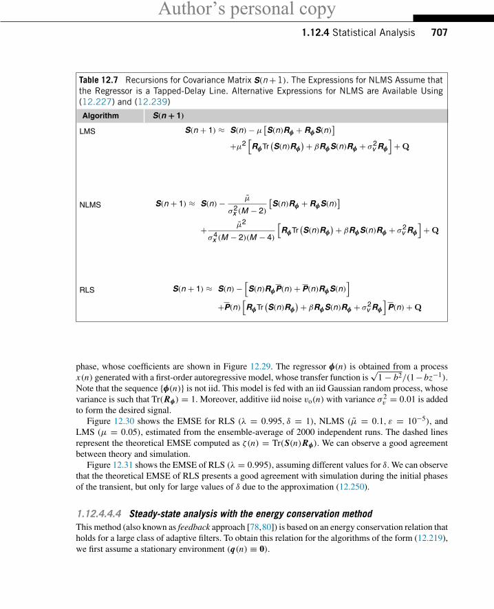
Author’s personal copy1.12.4 Statistical Analysis 707
Table 12.7 Recursions for Covariance Matrix S(n+1). The Expressions for NLMS Assume thatthe Regressor is a Tapped-Delay Line. Alternative Expressions for NLMS are Available Using(12.227) and (12.239)
Algorithm S(n + 1)
LMS S(n + 1) ≈ S(n)− μ [S(n)Rφ + RφS(n)]
+μ2[RφTr
(S(n)Rφ
)+ βRφS(n)Rφ + σ2v Rφ
]+Q
NLMS S(n + 1) ≈ S(n)− μ
σ2x (M − 2)
[S(n)Rφ + RφS(n)
]+ μ2
σ4x (M − 2)(M − 4)
[RφTr
(S(n)Rφ
)+ βRφS(n)Rφ + σ2v Rφ
]+Q
RLS S(n + 1) ≈ S(n)−[S(n)RφP(n)+ P(n)RφS(n)
]+P(n)
[RφTr
(S(n)Rφ
)+ βRφS(n)Rφ + σ2v Rφ
]P(n)+Q
phase, whose coefficients are shown in Figure 12.29. The regressor φ(n) is obtained from a processx(n) generated with a first-order autoregressive model, whose transfer function is
√1− b2/(1−bz−1).
Note that the sequence {φ(n)} is not iid. This model is fed with an iid Gaussian random process, whosevariance is such that Tr(Rφ) = 1. Moreover, additive iid noise vo(n) with variance σ 2
v = 0.01 is addedto form the desired signal.
Figure 12.30 shows the EMSE for RLS (λ = 0.995, δ = 1), NLMS (μ = 0.1, ε = 10−5), andLMS (μ = 0.05), estimated from the ensemble-average of 2000 independent runs. The dashed linesrepresent the theoretical EMSE computed as ζ(n) = Tr(S(n)Rφ). We can observe a good agreementbetween theory and simulation.
Figure 12.31 shows the EMSE of RLS (λ = 0.995), assuming different values for δ. We can observethat the theoretical EMSE of RLS presents a good agreement with simulation during the initial phasesof the transient, but only for large values of δ due to the approximation (12.250).
1.12.4.4.4 Steady-state analysis with the energy conservation methodThis method (also known as feedback approach [78,80]) is based on an energy conservation relation thatholds for a large class of adaptive filters. To obtain this relation for the algorithms of the form (12.219),we first assume a stationary environment (q(n) ≡ 0).
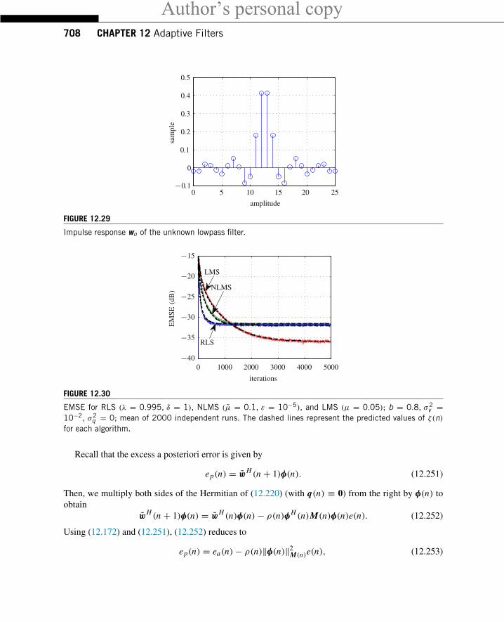
Author’s personal copy708 CHAPTER 12 Adaptive Filters
5 10 15 20 25−0.1
0
0
0.1
0.2
0.3
0.4
0.5
amplitude
sam
ple
FIGURE 12.29
Impulse response wo of the unknown lowpass filter.
20000 1000 3000 4000 5000
−15
−20
−25
−30
−35
−40
iterations
EM
SE(d
B)
RLS
LMS
NLMS
FIGURE 12.30
EMSE for RLS (λ = 0.995, δ = 1), NLMS (μ = 0.1, ε = 10−5), and LMS (μ = 0.05); b = 0.8, σ2v =
10−2, σ2q = 0; mean of 2000 independent runs. The dashed lines represent the predicted values of ζ(n)
for each algorithm.
Recall that the excess a posteriori error is given by
ep(n) = wH (n + 1)φ(n). (12.251)
Then, we multiply both sides of the Hermitian of (12.220) (with q(n) ≡ 0) from the right by φ(n) toobtain
wH (n + 1)φ(n) = wH (n)φ(n)− ρ(n)φH (n)M(n)φ(n)e(n). (12.252)
Using (12.172) and (12.251), (12.252) reduces to
ep(n) = ea(n)− ρ(n)‖φ(n)‖2M(n)e(n), (12.253)
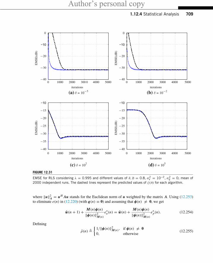
Author’s personal copy1.12.4 Statistical Analysis 709
−10
0
0 1000 2000 5000
−20
−30
−40
iterations
EM
SE(d
B)
(a) δ = 10−5
−10
0
300 0 4000 0 1000 2000 3000 4000 5000
−20
−30
−40
iterations
EM
SE(d
B)
(b) δ = 10−2
−10
0 1000 2000 3000 4000 5000
−15
−20
−25
−30
−35
−40
iterations
EM
SE(d
B)
(c) δ = 102
−10
0 1000 2000 3000 4000 5000
−15
−20
−25
−30
−35
−40
iterations
EM
SE(d
B)
(d) δ = 105
FIGURE 12.31
EMSE for RLS considering λ = 0.995 and different values of δ;b = 0.8, σ2v = 10−2, σ2
q = 0; mean of2000 independent runs. The dashed lines represent the predicted values of ζ(n) for each algorithm.
where ‖u‖2A = uH Au stands for the Euclidean norm of u weighted by the matrix A. Using (12.253)to eliminate e(n) in (12.220) (with q(n) ≡ 0) and assuming that φ(n) = 0, we get
w(n + 1)+ M(n)φ(n)
‖φ(n)‖2M(n)
e∗a(n) = w(n)+ M(n)φ(n)
‖φ(n)‖2M(n)
e∗p(n). (12.254)
Defining
ρ(n) �{
1/‖φ(n)‖2M(n), if φ(n) = 00, otherwise
(12.255)
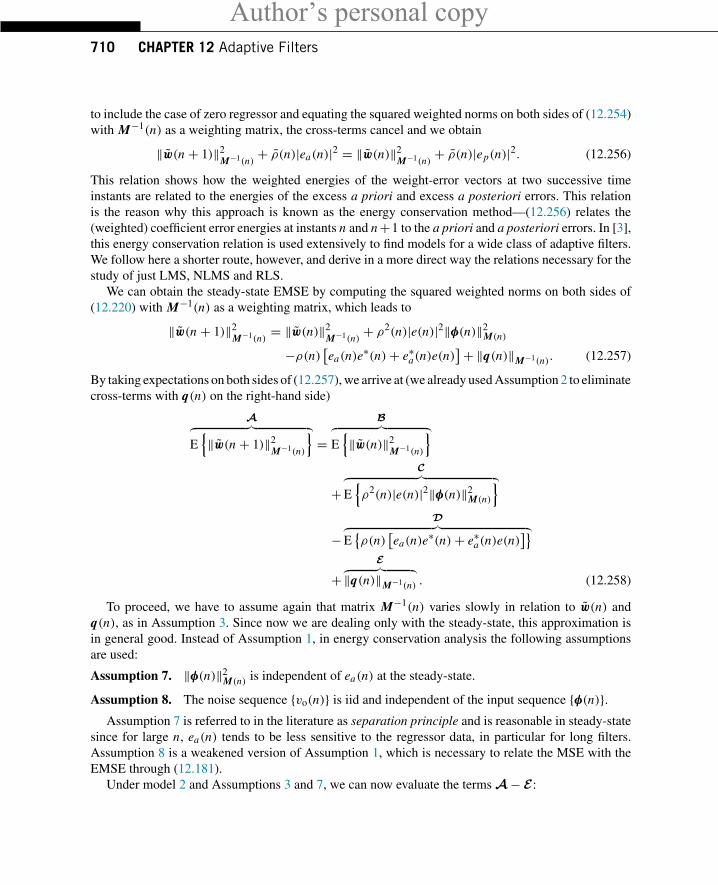
Author’s personal copy710 CHAPTER 12 Adaptive Filters
to include the case of zero regressor and equating the squared weighted norms on both sides of (12.254)with M−1(n) as a weighting matrix, the cross-terms cancel and we obtain
‖w(n + 1)‖2M−1(n)
+ ρ(n)|ea(n)|2 = ‖w(n)‖2M−1(n)+ ρ(n)|ep(n)|2. (12.256)
This relation shows how the weighted energies of the weight-error vectors at two successive timeinstants are related to the energies of the excess a priori and excess a posteriori errors. This relationis the reason why this approach is known as the energy conservation method—(12.256) relates the(weighted) coefficient error energies at instants n and n+1 to the a priori and a posteriori errors. In [3],this energy conservation relation is used extensively to find models for a wide class of adaptive filters.We follow here a shorter route, however, and derive in a more direct way the relations necessary for thestudy of just LMS, NLMS and RLS.
We can obtain the steady-state EMSE by computing the squared weighted norms on both sides of(12.220) with M−1(n) as a weighting matrix, which leads to
‖w(n + 1)‖2M−1(n)
= ‖w(n)‖2M−1(n)
+ ρ2(n)|e(n)|2‖φ(n)‖2M(n)
−ρ(n) [ea(n)e∗(n)+ e∗a(n)e(n)
]+ ‖q(n)‖M−1(n). (12.257)
By taking expectations on both sides of (12.257), we arrive at (we already used Assumption 2 to eliminatecross-terms with q(n) on the right-hand side)
A︷ ︸︸ ︷E{‖w(n + 1)‖2
M−1(n)
}=
B︷ ︸︸ ︷E{‖w(n)‖2
M−1(n)
}
+C︷ ︸︸ ︷
E{ρ2(n)|e(n)|2‖φ(n)‖2M(n)
}−
D︷ ︸︸ ︷E{ρ(n)
[ea(n)e
∗(n)+ e∗a(n)e(n)]}
+E︷ ︸︸ ︷
‖q(n)‖M−1(n) . (12.258)
To proceed, we have to assume again that matrix M−1(n) varies slowly in relation to w(n) andq(n), as in Assumption 3. Since now we are dealing only with the steady-state, this approximation isin general good. Instead of Assumption 1, in energy conservation analysis the following assumptionsare used:
Assumption 7. ‖φ(n)‖2M(n) is independent of ea(n) at the steady-state.
Assumption 8. The noise sequence {vo(n)} is iid and independent of the input sequence {φ(n)}.Assumption 7 is referred to in the literature as separation principle and is reasonable in steady-state
since for large n, ea(n) tends to be less sensitive to the regressor data, in particular for long filters.Assumption 8 is a weakened version of Assumption 1, which is necessary to relate the MSE with theEMSE through (12.181).
Under model 2 and Assumptions 3 and 7, we can now evaluate the terms A− E:
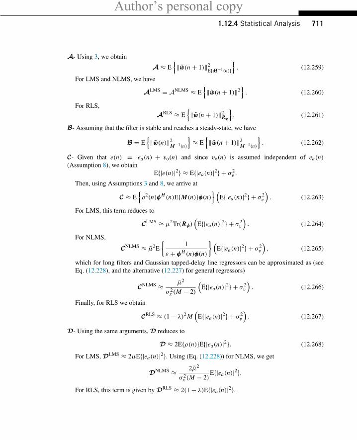
Author’s personal copy1.12.4 Statistical Analysis 711
A- Using 3, we obtain
A ≈ E{‖w(n + 1)‖2
E{M−1(n)}}. (12.259)
For LMS and NLMS, we have
ALMS = ANLMS ≈ E{‖w(n + 1)‖2
}. (12.260)
For RLS,ARLS ≈ E
{‖w(n + 1)‖2Rφ
}. (12.261)
B- Assuming that the filter is stable and reaches a steady-state, we have
B = E{‖w(n)‖2
M−1(n)
}≈ E
{‖w(n + 1)‖2
M−1(n)
}. (12.262)
C- Given that e(n) = ea(n) + vo(n) and since vo(n) is assumed independent of ea(n)(Assumption 8), we obtain
E{|e(n)|2} ≈ E{|ea(n)|2} + σ 2v .
Then, using Assumptions 3 and 8, we arrive at
C ≈ E{ρ2(n)φH (n)E{M(n)}φ(n)
} (E{|ea(n)|2} + σ 2
v
). (12.263)
For LMS, this term reduces to
CLMS ≈ μ2Tr(Rφ)(
E{|ea(n)|2} + σ 2v
). (12.264)
For NLMS,
CNLMS ≈ μ2E
{1
ε + φH (n)φ(n)
}(E{|ea(n)|2} + σ 2
v
), (12.265)
which for long filters and Gaussian tapped-delay line regressors can be approximated as (seeEq. (12.228), and the alternative (12.227) for general regressors)
CNLMS ≈ μ2
σ 2x (M − 2)
(E{|ea(n)|2} + σ 2
v
). (12.266)
Finally, for RLS we obtain
CRLS ≈ (1− λ)2 M(
E{|ea(n)|2} + σ 2v
). (12.267)
D- Using the same arguments, D reduces to
D ≈ 2E{ρ(n)}E{|ea(n)|2}. (12.268)
For LMS, DLMS ≈ 2μE{|ea(n)|2}. Using (Eq. (12.228)) for NLMS, we get
DNLMS ≈ 2μ2
σ 2x (M − 2)
E{|ea(n)|2}.
For RLS, this term is given by DRLS ≈ 2(1− λ)E{|ea(n)|2}.
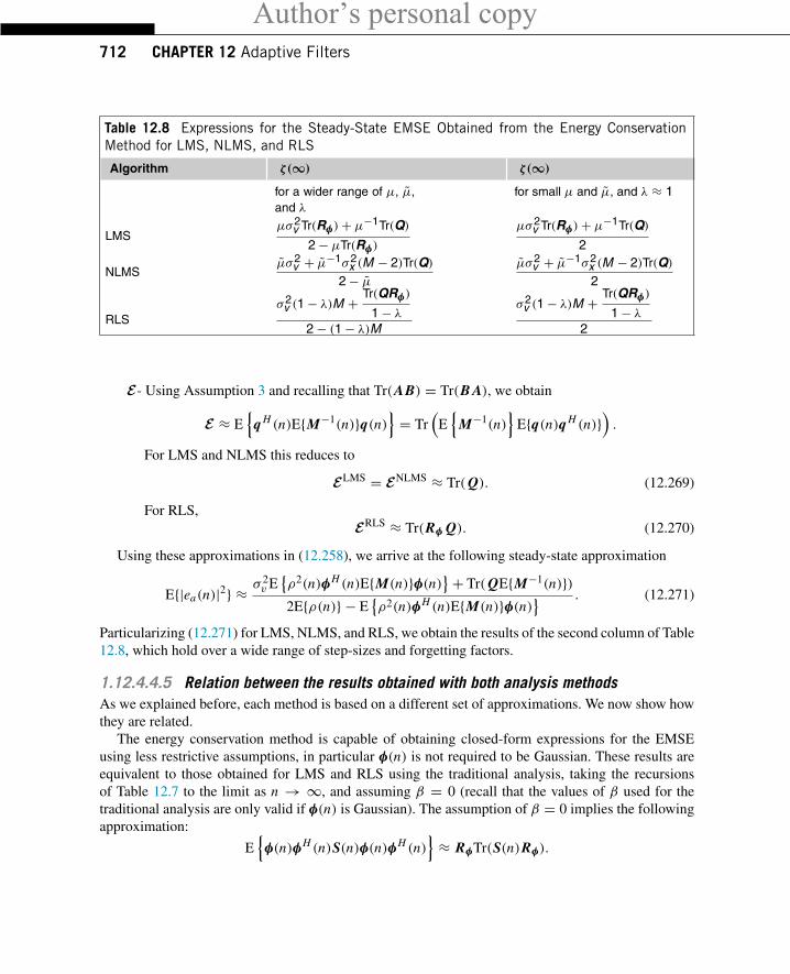
Author’s personal copy712 CHAPTER 12 Adaptive Filters
Table 12.8 Expressions for the Steady-State EMSE Obtained from the Energy ConservationMethod for LMS, NLMS, and RLS
Algorithm ζ(∞) ζ(∞)
for a wider range of μ, μ,and λ
for small μ and μ, and λ ≈ 1
LMSμσ2
v Tr(Rφ)+ μ−1Tr(Q)
2− μTr(Rφ)
μσ2v Tr(Rφ)+ μ−1Tr(Q)
2
NLMSμσ2
v + μ−1σ2x (M − 2)Tr(Q)
2− μμσ2
v + μ−1σ2x (M − 2)Tr(Q)2
RLSσ2
v (1− λ)M +Tr(QRφ)
1− λ2− (1− λ)M
σ2v (1− λ)M +
Tr(QRφ)
1− λ2
E- Using Assumption 3 and recalling that Tr(AB) = Tr(B A), we obtain
E ≈ E{
q H (n)E{M−1(n)}q(n)}= Tr
(E{
M−1(n)}
E{q(n)q H (n)}).
For LMS and NLMS this reduces to
ELMS = ENLMS ≈ Tr(Q). (12.269)
For RLS,ERLS ≈ Tr(Rφ Q). (12.270)
Using these approximations in (12.258), we arrive at the following steady-state approximation
E{|ea(n)|2} ≈ σ 2v E
{ρ2(n)φH (n)E{M(n)}φ(n)}+ Tr(QE{M−1(n)})2E{ρ(n)} − E
{ρ2(n)φH (n)E{M(n)}φ(n)} . (12.271)
Particularizing (12.271) for LMS, NLMS, and RLS, we obtain the results of the second column of Table12.8, which hold over a wide range of step-sizes and forgetting factors.
1.12.4.4.5 Relation between the results obtained with both analysis methodsAs we explained before, each method is based on a different set of approximations. We now show howthey are related.
The energy conservation method is capable of obtaining closed-form expressions for the EMSEusing less restrictive assumptions, in particular φ(n) is not required to be Gaussian. These results areequivalent to those obtained for LMS and RLS using the traditional analysis, taking the recursionsof Table 12.7 to the limit as n → ∞, and assuming β = 0 (recall that the values of β used for thetraditional analysis are only valid if φ(n) is Gaussian). The assumption of β = 0 implies the followingapproximation:
E{φ(n)φH (n)S(n)φ(n)φH (n)
}≈ RφTr(S(n)Rφ).
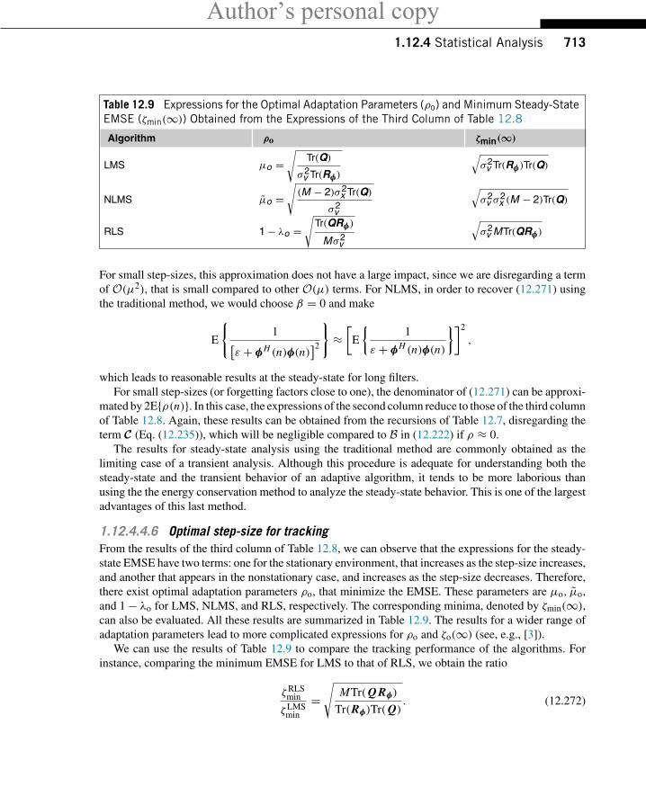
Author’s personal copy1.12.4 Statistical Analysis 713
Table 12.9 Expressions for the Optimal Adaptation Parameters (ρo) and Minimum Steady-StateEMSE (ζmin(∞)) Obtained from the Expressions of the Third Column of Table 12.8
Algorithm ρo ζmin(∞)
LMS μo =√
Tr(Q)
σ2v Tr(Rφ)
√σ2
v Tr(Rφ)Tr(Q)
NLMS μo =√(M − 2)σ2
x Tr(Q)
σ2v
√σ2
v σ2x (M − 2)Tr(Q)
RLS 1− λo =√
Tr(QRφ)
Mσ2v
√σ2
v MTr(QRφ)
For small step-sizes, this approximation does not have a large impact, since we are disregarding a termof O(μ2), that is small compared to other O(μ) terms. For NLMS, in order to recover (12.271) usingthe traditional method, we would choose β = 0 and make
E
{1[
ε + φH (n)φ(n)]2
}≈[
E
{1
ε + φH (n)φ(n)
}]2
,
which leads to reasonable results at the steady-state for long filters.For small step-sizes (or forgetting factors close to one), the denominator of (12.271) can be approxi-
mated by 2E{ρ(n)}. In this case, the expressions of the second column reduce to those of the third columnof Table 12.8. Again, these results can be obtained from the recursions of Table 12.7, disregarding theterm C (Eq. (12.235)), which will be negligible compared to B in (12.222) if ρ ≈ 0.
The results for steady-state analysis using the traditional method are commonly obtained as thelimiting case of a transient analysis. Although this procedure is adequate for understanding both thesteady-state and the transient behavior of an adaptive algorithm, it tends to be more laborious thanusing the the energy conservation method to analyze the steady-state behavior. This is one of the largestadvantages of this last method.
1.12.4.4.6 Optimal step-size for trackingFrom the results of the third column of Table 12.8, we can observe that the expressions for the steady-state EMSE have two terms: one for the stationary environment, that increases as the step-size increases,and another that appears in the nonstationary case, and increases as the step-size decreases. Therefore,there exist optimal adaptation parameters ρo, that minimize the EMSE. These parameters are μo, μo,and 1− λo for LMS, NLMS, and RLS, respectively. The corresponding minima, denoted by ζmin(∞),can also be evaluated. All these results are summarized in Table 12.9. The results for a wider range ofadaptation parameters lead to more complicated expressions for ρo and ζo(∞) (see, e.g., [3]).
We can use the results of Table 12.9 to compare the tracking performance of the algorithms. Forinstance, comparing the minimum EMSE for LMS to that of RLS, we obtain the ratio
ζRLSmin
ζLMSmin
=√
MTr(Q Rφ)
Tr(Rφ)Tr(Q). (12.272)
Author’s personal copy714 CHAPTER 12 Adaptive Filters
Clearly, the results of this comparison depend on the environment. There are situations where RLS hassuperior tracking capability compared to LMS, and vice versa. This is highlighted considering threedifferent choices for matrix Q. It can be shown [81] that
i. If Q is a multiple of I : the performance of LMS is similar to that of RLS;ii. If Q is a multiple of Rφ : LMS is superior; and
iii. If Q is a multiple of R−1φ : RLS is superior.
These choices for Q do not model practical situations, but they highlight that, even though the conver-gence rate of RLS is in general much higher than that of LMS, this advantage, unexpectedly, does notnecessarily follow to the problem of tracking a slowly-varying parameter vector.
Example 4. To verify the accuracy of the expressions of Tables 12.8 and 12.9, we use the LMS,NLMS, and RLS filters to identify the same lowpass FIR system of Figure 12.29. Now, the environmentis assumed nonstationary with Q = 10−6 I . The input signal and minimum MSE (σ 2
v ) are the same ofExample 3.
Figure 12.32 shows the measured steady-state EMSE with varying adaptation factors considering thetheoretical and experimental results for LMS, NLMS, and RLS. Each value of experimental EMSE wasobtained from the ensemble-average of 100 independent runs. The theoretical minimum EMSE predictedby the expressions of Table 12.9 are ζLMS
o (∞) = ζRLSo (∞) = −32.9251 dB and ζNLMS
o (∞) =−33.0989 dB, which correspond to the optimal adaptation parameters μo = 5.1× 10⁻², μo = 4.9×10⁻² and 1− λo = 2 × 10⁻³ (λo = 0.998). The experimental values for ζmin(∞) and ρo are close tothe predicted by the expressions of Table 12.9 as shown in Figure 12.32.
Example 5. Again, we consider a system identification application but with the initial optimal solutiongiven by
wTo (0) = [ 0.5349 0.9527 −0.9620 −0.0158 −0.1254 ].
The input signal is assumed to be colored Gaussian noise with variance σ 2x = 0.2. This signal is obtained
from the filtering of a white Gaussian noise by a first-order autoregressive model (b = 0.8). We alsoassume that the minimum MSE is σ 2
v = 0.01.As predicted by (12.272), the performance of RLS and LMS are similar when Q = σ 2
q I . Thus,assuming Q = 10−6 I , we computed μo and λo from the expressions of Table 12.9 and used theseparameters in the adaptation, such that the same minimum EMSE could be achieved by both algorithms inthis situation. Figure 12.33 shows the EMSE estimated from the ensemble-average of 5000 independentruns for RLS (λ = λo = 0.9955, δ = 4.5 × 10⁻³) and LMS (μ = μo = 0.0224). At every 7 × 10⁴
iterations, the nonstationary environment is changed. During the first 7× 10⁴ iterations, Q = 10−6 Rφ
and LMS presents a slightly better tracking performance than that of RLS. When Q = 10−6 R−1φ , this
behavior changes: RLS becomes better than LMS. Finally for Q = 10−6 I , RLS and LMS presentsimilar performance. The dashed lines represent the theoretical values of ζ(∞) for each algorithm,predicted from the expressions of the second column of Table 12.8.
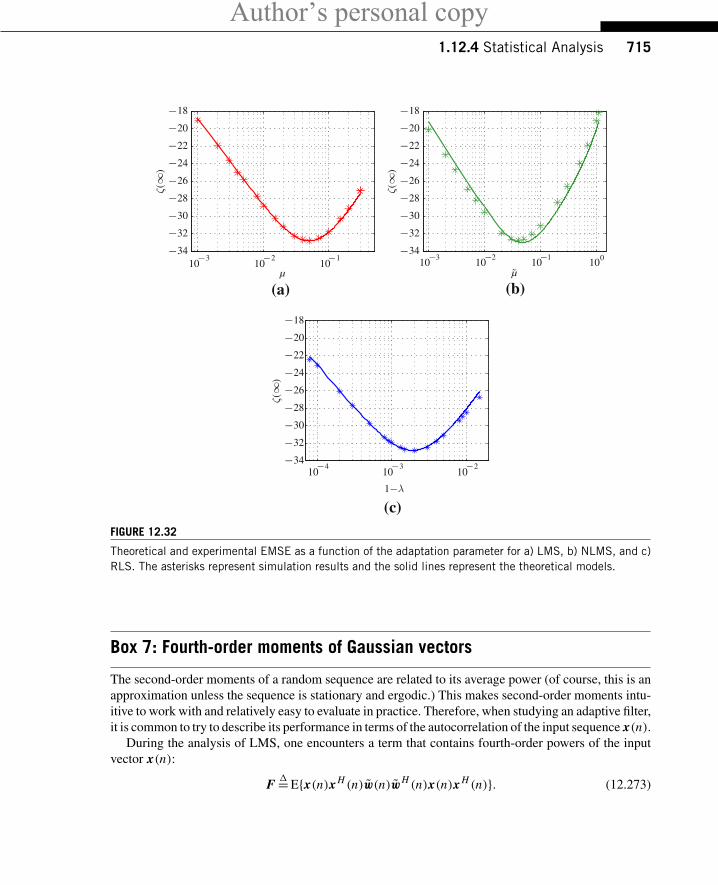
Author’s personal copy1.12.4 Statistical Analysis 715
−18
−20
−22
−24
−26
−28
−30
−32
−34 −3 −2 −1101010
(a)µ
ζ(∞
)
−18
−20
−22
−24
−26
−28
−30
−32
−34 −3 −2 −1 010101010
(b)µ
ζ(∞
)
−18
−20
−22
−24
−26
−28
−30
−32
−34 −4 −3 −2101010
(c)1−λ
ζ(∞
)
FIGURE 12.32
Theoretical and experimental EMSE as a function of the adaptation parameter for a) LMS, b) NLMS, and c)RLS. The asterisks represent simulation results and the solid lines represent the theoretical models.
Box 7: Fourth-order moments of Gaussian vectors
The second-order moments of a random sequence are related to its average power (of course, this is anapproximation unless the sequence is stationary and ergodic.) This makes second-order moments intu-itive to work with and relatively easy to evaluate in practice. Therefore, when studying an adaptive filter,it is common to try to describe its performance in terms of the autocorrelation of the input sequence x(n).
During the analysis of LMS, one encounters a term that contains fourth-order powers of the inputvector x(n):
F�=E{x(n)x H (n)w(n)wH (n)x(n)x H (n)}. (12.273)
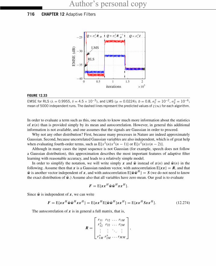
Author’s personal copy716 CHAPTER 12 Adaptive Filters
0 0.5 1 1.5 2
×105
−25
−30
−35
−40
iterations
EM
SE(d
B)
RLS
Q = σ2v R −1
φ Q = σ2v I
LMS
Q = σ2v R φ
FIGURE 12.33
EMSE for RLS (λ = 0.9955, δ = 4.5× 10⁻³), and LMS (μ = 0.0224); b = 0.8, σ2v = 10−2, σ2
q = 10−6;mean of 5000 independent runs. The dashed lines represent the predicted values of ζ(∞) for each algorithm.
In order to evaluate a term such as this, one needs to know much more information about the statisticsof x(n) than is provided simply by its mean and autocorrelation. However, in general this additionalinformation is not available, and one assumes that the signals are Gaussian in order to proceed.
Why not any other distribution? First, because many processes in Nature are indeed approximatelyGaussian. Second, because uncorrelated Gaussian variables are also independent, which is of great helpwhen evaluating fourth-order terms, such as E{x2(n)x2(n − 1)} or E{x3(n)x(n − 2)}.
Although in many cases the input sequence is not Gaussian (for example, speech does not followa Gaussian distribution), this approximation describes the most important features of adaptive filterlearning with reasonable accuracy, and leads to a relatively simple model.
In order to simplify the notation, we will write simply x and w instead of x(n) and w(n) in thefollowing. Assume then that x is a Gaussian random vector, with autocorrelation E{xx} = R, and thatw is another vector independent of x, and with autocorrelation E{wwH } = S (we do not need to knowthe exact distribution of w.) Assume also that all variables have zero mean. Our goal is to evaluate
F = E{xx H wwH xx H }.Since w is independent of x, we can write
F = E{xx H wwH xx H } = E{xx H E{wwH }xx H } = E{xx H Sxx H }. (12.274)
The autocorrelation of x is in general a full matrix, that is,
R =
⎡⎢⎢⎢⎣r11 r12 . . . r1M
r∗12 r22 . . . r2M...
.... . .
...
r∗1M r∗2M . . . rM M
⎤⎥⎥⎥⎦ ,
Author’s personal copy1.12.5 Extensions and Current Research 717
that is, in general the elements of x are correlated. R has hermitian symmetry and is non-negativedefinite, which implies that there exists a unitary matrix U such that
U H RU = � =
⎡⎢⎢⎢⎣λ1 0 . . . 00 λ2 . . . 0...
.... . .
...
0 0 . . . λM
⎤⎥⎥⎥⎦ ,where λi ≥ 0 for i = 1, . . . ,M . Define x′ = U H x. Then E{x′x′H } = E{U H xx H U} = U H E{xx H }U = �, and we see that the entries of x′ are uncorrelated. Since x is Gaussian, and a linear transformationof a Gaussian vector is also Gaussian, this means that the entries of x′ are independent of each other.Multiplying (12.274) by U H on the left and U on the right, and recalling that U H U = UU H = I , weobtain
F′ �=U H FU = E{U H xx H UU H︸ ︷︷ ︸=I
S UU H︸ ︷︷ ︸=I
xx H U} = E{x′x′H U H SU x′x′H }.
Defining S = U H SU , we can expand F in terms of the elements s′i j of S and x ′k of x′. Each elementof F will have terms of the form
E{x ′k1x ′k2 x ′∗k3 x ′∗k4
}s′i j .
If the signals are real, then, as x ′k1is independent of x ′k2
if k1 = k2, these expected values will be nonzeroonly if k1 = k2 = k3 = k4 or if k1 = k3 and k2 = k4, or k1 = k4 and k2 = k3, or if k1 = k2 and k3 = k4.Evaluating all such terms that appear in the expression for F′ will result in
F|real signals = RTr(SR)+ 2RSR. (12.275)
If, on the other hand, the signals are complex-valued, then we need to know how the real and imaginaryparts of each entry of x relate to each other. One common assumption is that x is circularly-Gaussian.We explain more about this in Section 1.12.2.2.1. For now, we only remark that if this is the case, thereal and imaginary parts of each entry of x and of x′ are such that E{x2
k } = E{x ′2k } = 0 for all k (notethat E{|xk |2} = rkk,E{|x ′k |2} = λk are still nonzero.) This will result in a different expression for F:
F|complex signals = RTr(SR)+ RSR. (12.276)
1.12.5 Extensions and current researchIn this section we briefly describe some important extensions to the basic adaptive filtering algorithms,as well as some promising current research topics. The intention is not to describe in any detail allthese techniques, but rather to give a list of key references where the interested reader may find moreinformation.
It is usual when starting such lists to put a disclaimer, that the authors do not claim to have includedall the important contributions, nor that their list is really of the most important contributions to an area.

Author’s personal copy718 CHAPTER 12 Adaptive Filters
This is not intended for legal purposes, nor false modesty: the size of the literature is indeed so large(a search on “adaptive filter” on Google gives over one million hits) that we cannot claim to know withcertainty the best of it all. We included therefore the techniques that we found useful during our ownresearch and experience, which is perforce limited.
1.12.5.1 Finite-precision arithmeticAny operation made using finite-precision arithmetic may involve errors. For example, the product ofa = 0.957 and b = 0.542 would result in c = 0.518694. However, if all numbers were stored keepingonly three digits, the final result would be c = 0.519, with an error of c − c = −3.06× 10⁻⁴ [82,83].These quantization errors will accumulate and modify the behavior of an adaptive filter in importantways. A precise analysis of the effect of quantization errors is quite complicated, since these errors arehighly nonlinear functions of the variables.
When finite-precision arithmetic effects are studied, it is usually important to know exactly how andin which order the arithmetic operations are performed. In particular, the exact numerical representationused is important: fixed-point vs. floating-point, truncation vs. rounding, etc. For this reason, it ismore difficult to perform analyses that are equally valid for a large class of filters. The most importantdifferences are between gradient-based algorithms (i.e., algorithms similar to LMS and NLMS) andHessian-based algorithms (i.e., algorithms similar to RLS). We will give references to works treatingboth cases, starting with LMS.
1.12.5.1.1 Finite-precision effects in LMSThe simplest models for adaptive filters in finite-precision arithmetic treat the quantization error asrandom noise, uniformly distributed and independent of all variables [84–87]. These models show thatthe quantization errors will add another term to the EMSE. However, this term does not converge tozero when the step-size is reduced to zero, even in a stationary environment: quite the opposite, it isinversely proportional to the step-size (similar to the EMSE in a nonstationary environment).
Another important undesirable effect is that the product μe(n) may be rounded down to zero whene(n) becomes small (underflow), virtually stopping the adaptation. When the step-size is small, thismay happen when the filter is rather far from the optimum solution. Therefore, there is an optimumvalue for the step-size—neither too large, to avoid increasing the misadjustment, neither too small, toavoid underflow and excessive growth of the EMSE. A similar effect happens in RLS [1, p. 595].
This underflow problem, which is usually known as stopping phenomenon, was studied in more detailin [88–91], using a nonlinear model. These works show that the adaptation does not really stop, butrather convergence is reduced to a very low rate. Note that this phenomenon is less important in floating-point arithmetic, since floating-point is able to represent much smaller numbers without underflow thanfixed-point arithmetic.
Finite precision effects may have worse consequences, in particular they may make the adaptivefilter unstable. In the case of LMS, this phenomenon is rare, and will only happen when the regressorsequence {φ} has a very ill-conditioned covariance matrix, and the noise vo has a nonzero mean (thisnonzero mean may itself appear due to quantization errors) [92–94]. This problem is not difficult tosolve, using regularization as described in Section 1.12.5.2. The problem of numerical stability in RLSis much more serious and harder to solve, and has received much attention, as we see next.
Author’s personal copy1.12.5 Extensions and Current Research 719
In addition to studying the effect of quantization errors in the performance of an adaptive filter, anotherimportant topic is how to reduce the computational cost of a filter, taking advantage of implementationdetails. One such approach is to replace the error e(n) in the LMS recursion by its sign, i.e., to use therecursion
w(n + 1) = w(n)+ μsign(e(n)
)φ(n), (12.277)
where sign(·) is the sign function, defined by
sign(e) =
⎧⎨⎩1, if e > 0,0, if e = 0,−1, if e < 0.
(12.278)
The resulting algorithm, known as sign-LMS, has a smaller computational cost, if μ is restricted tobe a power of two, that is, if μ = 2k for an integer (usually negative) k. In this case, μsign
(e(n)
)is
always equal to ±2k (or zero), and the product[μsign
(e(n)
)]φ(n) can be implemented in fixed-point
arithmetic as M shifts, instead of M multiplications. In floating-point arithmetic, the multiplicationsare replaced by sums, since we would need to add k to the exponent terms of all entries of φ(n). Thisalgorithm is very robust (see also Section 1.12.5.4), although its convergence rate under Gaussian inputsis considerably slower than that of LMS. Sign-LMS was thoroughly studied in [81,95–98].
Another possibility, that works surprisingly well, reducing the computational cost with only a slightdecrease in convergence speed is the power-of-two LMS algorithm [99]. In it, the error is rounded tothe nearest power of two, using the function:
f(e) =
⎧⎨⎩sign(e), |e| ≥ 1,sign(e)2�ln (|e|)�, 2−B+1 ≤ |e| < 1,0, |e| < 2−B+1,
where B is the number of bits used to represent the error, and �x� returns the largest integer smallerthan x . In this case, μ should also be a power of two.
1.12.5.1.2 Finite-precision effects in RLSAs we briefly described in Section 1.12.3.3.1, the conventional RLS is numerically unstable in finiteprecision arithmetic and has O(M2) complexity. To solve these problems, different versions of RLSwere proposed in the literature. Many of these versions are based on coordinate transformations of thestate-space representation of the conventional RLS algorithm. This representation can be obtained byreplacing k(n) by P(n)φ(n) in(12.166), i.e.,
w(n + 1) = λP(n)rdφ(n − 1)+ P(n)φ(n)d∗(n). (12.279)
Recalling that w(n) = P(n − 1)rdφ(n − 1), we can replace rdφ(n − 1) in (12.279) as a function ofP−1(n − 1) and w(n), which leads to
w(n + 1) = λP(n)P−1(n − 1)w(n)+ P(n)φ(n)d∗(n). (12.280)
Author’s personal copy720 CHAPTER 12 Adaptive Filters
This equation in conjunction with the definition of the a priori error e(n) characterize the adaptationand filtering operations of the RLS algorithm and constitute its state-space representation, i.e.,
[w(n + 1)
e∗(n)
]=[λP(n)P−1(n − 1) P(n)φ(n)−φH (n) 1
] [w(n)d∗(n)
]. (12.281)
In this representation, w(n) is the state, e∗(n) is the output, and d∗(n) is the input.Performing a coordinate transformation, (12.281) can be transformed to an unlimited number of
systems with the same input-output relation, and hence solving the same least-squares problem (that is,the output error is always the same). Although all these realizations are equivalent in infinite precisionarithmetic, the numerical behavior will vary from one coordinate system to another. Thus, the numericalinstability of the conventional RLS can be avoided by choosing a convenient transformation of (12.281)[40,100].
An alternative method of implementing RLS is based on the QR decomposition (QRD) [14] totriangularize the input data matrix. The main advantages of QRD-RLS-based algorithms are the possi-bility of implementation in systolic arrays (e.g., [101]) and the improved numerical behavior in finiteprecision arithmetic. Some versions require O(M2) operations per iteration, but others have a reducedcomputational cost of O(M). The low-cost versions of QRD-RLS algorithms are known as fast-QRalgorithms. Some important references on this subject are [38,101–116]. A good tutorial on QRD-RLS-based algorithms can be found in [43], where the most recent developments as well as the basic conceptsare covered.
Another important class of fast algorithms solves the least-squares problem in a recursive form basedon the lattice realization. These algorithms are very attractive due to the possible modular implementationand low cost (O(M)). Lattice-RLS-based algorithms are derived by solving the forward and backwardlinear prediction problems and require time-update and order-update recursions. They explore the time-shift property of the input signal vector (such as in (12.113)) and do not compute explicitly the filterweights. Recall that many applications do not require the computation of the filter weights and haveregressors that satisfy the time-shift property as, for example, channel equalization and interferencecancellation (see Section 1.12.1.3). In these applications, a fast RLS algorithm can be a reasonablechoice since it presents a good tradeoff between convergence rate and computational cost. One ofthese algorithms is the modified EF-LSL (error-feedback least-squares lattice algorithm) that presentsreliable numerical properties when implemented in finite-precision arithmetic [5]. This algorithm wasproposed for echo-cancellation applications and was used in the example of Section 1.12.1.1. Somelattice-RLS-based algorithms can be found in the references [5,117–124].
More recently, lattice-RLS algorithms have been generalized to filter structures other than tapped-delay lines, in particular, to Laguerre filters [125–127].
Other fast algorithms that solve the least-squares problem in a recursive form are the fast transversalRLS (FTRLS) algorithms. Unlike the lattice-based algorithms, the FTRLS algorithms require onlytime-recursive equations and therefore, compute explicitly the filter weights. The main drawback ofthese algorithms is that they are very sensitive to quantization effects and become unstable if certainactions are not taken [1]. The list of fast transversal RLS algorithms is vast. Some of the most importantversions can be found in the references [128–134].
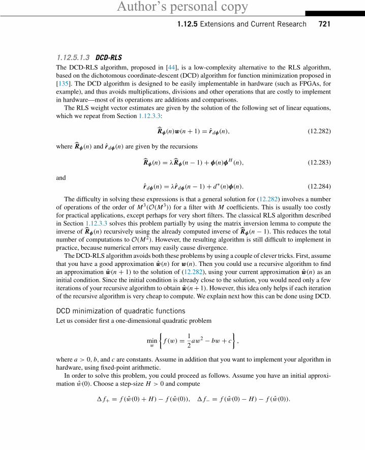
Author’s personal copy1.12.5 Extensions and Current Research 721
1.12.5.1.3 DCD-RLSThe DCD-RLS algorithm, proposed in [44], is a low-complexity alternative to the RLS algorithm,based on the dichotomous coordinate-descent (DCD) algorithm for function minimization proposed in[135]. The DCD algorithm is designed to be easily implementable in hardware (such as FPGAs, forexample), and thus avoids multiplications, divisions and other operations that are costly to implementin hardware—most of its operations are additions and comparisons.
The RLS weight vector estimates are given by the solution of the following set of linear equations,which we repeat from Section 1.12.3.3:
Rφ(n)w(n + 1) = rdφ(n), (12.282)
where Rφ(n) and rdφ(n) are given by the recursions
Rφ(n) = λRφ(n − 1)+ φ(n)φH (n), (12.283)
andrdφ(n) = λrdφ(n − 1)+ d∗(n)φ(n). (12.284)
The difficulty in solving these expressions is that a general solution for (12.282) involves a numberof operations of the order of M3(O(M3)) for a filter with M coefficients. This is usually too costlyfor practical applications, except perhaps for very short filters. The classical RLS algorithm describedin Section 1.12.3.3 solves this problem partially by using the matrix inversion lemma to compute theinverse of Rφ(n) recursively using the already computed inverse of Rφ(n − 1). This reduces the totalnumber of computations to O(M2). However, the resulting algorithm is still difficult to implement inpractice, because numerical errors may easily cause divergence.
The DCD-RLS algorithm avoids both these problems by using a couple of clever tricks. First, assumethat you have a good approximation w(n) for w(n). Then you could use a recursive algorithm to findan approximation w(n + 1) to the solution of (12.282), using your current approximation w(n) as aninitial condition. Since the initial condition is already close to the solution, you would need only a fewiterations of your recursive algorithm to obtain w(n+1). However, this idea only helps if each iterationof the recursive algorithm is very cheap to compute. We explain next how this can be done using DCD.
DCD minimization of quadratic functionsLet us consider first a one-dimensional quadratic problem
minw
{f (w) = 1
2aw2 − bw + c
},
where a > 0, b, and c are constants. Assume in addition that you want to implement your algorithm inhardware, using fixed-point arithmetic.
In order to solve this problem, you could proceed as follows. Assume you have an initial approxi-mation w(0). Choose a step-size H > 0 and compute
� f+ = f (w(0)+ H)− f (w(0)), � f− = f (w(0)− H)− f (w(0)).
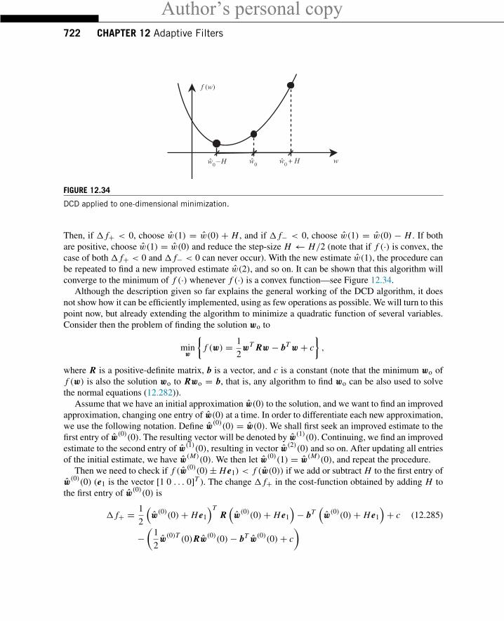
Author’s personal copy722 CHAPTER 12 Adaptive Filters
w0−H w0 + Hw0w
f (w)
FIGURE 12.34
DCD applied to one-dimensional minimization.
Then, if � f+ < 0, choose w(1) = w(0) + H , and if � f− < 0, choose w(1) = w(0) − H . If bothare positive, choose w(1) = w(0) and reduce the step-size H ← H/2 (note that if f (·) is convex, thecase of both � f+ < 0 and � f− < 0 can never occur). With the new estimate w(1), the procedure canbe repeated to find a new improved estimate w(2), and so on. It can be shown that this algorithm willconverge to the minimum of f (·) whenever f (·) is a convex function—see Figure 12.34.
Although the description given so far explains the general working of the DCD algorithm, it doesnot show how it can be efficiently implemented, using as few operations as possible. We will turn to thispoint now, but already extending the algorithm to minimize a quadratic function of several variables.Consider then the problem of finding the solution wo to
minw
{f (w) = 1
2wT Rw − bT w + c
},
where R is a positive-definite matrix, b is a vector, and c is a constant (note that the minimum wo off (w) is also the solution wo to Rwo = b, that is, any algorithm to find wo can be also used to solvethe normal equations (12.282)).
Assume that we have an initial approximation w(0) to the solution, and we want to find an improvedapproximation, changing one entry of w(0) at a time. In order to differentiate each new approximation,we use the following notation. Define w
(0)(0) = w(0). We shall first seek an improved estimate to the
first entry of w(0)(0). The resulting vector will be denoted by w
(1)(0). Continuing, we find an improved
estimate to the second entry of w(1)(0), resulting in vector w
(2)(0) and so on. After updating all entries
of the initial estimate, we have w(M)(0). We then let w
(0)(1) = w
(M)(0), and repeat the procedure.
Then we need to check if f (w(0)(0)± H e1) < f (w(0)) if we add or subtract H to the first entry of
w(0)(0) (e1 is the vector [1 0 . . . 0]T ). The change � f+ in the cost-function obtained by adding H to
the first entry of w(0)(0) is
� f+ = 1
2
(w(0)(0)+ H e1
)TR(w(0)(0)+ H e1
)− bT
(w(0)(0)+ H e1
)+ c (12.285)
−(
1
2w(0)T
(0)Rw(0)(0)− bT w
(0)(0)+ c
)
Author’s personal copy1.12.5 Extensions and Current Research 723
= H eT1 Rw
(0)(0)+ 1
2H2eT
1 Re1 − H bT e1. (12.286)
Similarly, the variation � f− obtained from subtracting H from the first entry of w(0) is
� f− = −H eT1 Rw
(0)(0)+ 1
2H2eT
1 Re1 + H bT e1. (12.287)
Therefore, we should make
w(1)(0) =
⎧⎪⎨⎪⎩w(0)(0)+ H e1, if � f+ < 0,
w(0)(0)− H e1, if � f− < 0,
w(0)(0), otherwise.
(12.288)
The same steps can be repeated for the second entry of w(1)(0) and so on, that is, we can update the
(m + 1)th entry of w(m)(0) to obtain a new approximation w
(m+1)(0) for m = 0, . . . ,M − 1. After
obtaining w(M)(0), we have updated all entries of w(0). We can then make w
(0)(1) = w
(M)(0) and
repeat the procedure. However, if no update is made for m = 1, . . . ,M , before repeating we decreasethe step H by a factor of two (i.e., H ← H/2). By reducing H only when no update is necessary forany entry of the vector, we avoid problems that would appear if the initial value of H were too small.
Implemented as described so far, the algorithm has a high computational cost. For example, for theevaluation of � f+ at each step we must
• Evaluate eTm Rw
(m−1)(i). This is equivalent to multiplying the mth row of R by w
(m−1)(i), involving
M multiplications and M − 1 additions.• Multiply −eT
m Rw(m−1)
(i) + bT em by H and add the result to (H2/2)Rm,m (Rm,m is the element(m,m) of R). This requires 2 multiplications and 2 additions, assuming H2/2 is pre-computed.
The same steps would be necessary for the computation of� f−. Note that all these computations wouldhave to be repeated at each step, therefore the update of all entries of w
(0)(i) would require more than
M2 multiplications.However, the number of computations can be reduced substantially, if we take advantage of some
properties of hardware implementations of arithmetic operations, as we describe next. Assume in thefollowing that all variables are fixed-point binary numbers (see Box 8).
First, we can avoid the computation of Rw(m−1)
(i) by introducing a residue vector that is updatedat each step. Let r(0)(0) = b − Rw
(0)(0) be the initial residue vector. Note that this is the residue of
solving Rw = b using w(0)(0) as an approximation to the solution.
At the end of the first step, w(0)(0) is updated as in (12.288). Since only one entry of w
(0)(0) is
changed, the modification in the residue is simple to evaluate
r(1)(0) = b− Rw(1)(0) =
⎧⎨⎩b− R(w(0)
(0)+ H e1) = r(0)(0)− H Re1, if � f+ < 0,b− R(w(0)
(0)− H e1) = r(0)(0)+ H Re1, if � f− < 0,r(0)(0), otherwise.
(12.289)
This still requires M multiplications (H multiplied by the first column of R). However, if H is apower of two, that is, if H = 2k for some integer k, than the computation of r(1)(0) in fixed-point
Author’s personal copy724 CHAPTER 12 Adaptive Filters
arithmetic requires only M shifts and M additions, which are much easier to implement in hardwarethan multiplications. Moreover, if both � f+ and � f− are positive, no update is necessary.
Next, we note that it is not really necessary to compute both � f+ and � f−: from (12.286) and(12.287), when updating the mth element of w
(m−1)(i) at step i , we have
� f+ = −H eTm r(m−1)(i)+ 1
2H2eT
m Rem = −Hr (m−1)m (i)+ 1
2H2 Rm,m, (12.290)
where r (m−1)m (i) is the mth entry of the residue vector r(m−1)(i), r(0)(i + 1)
�= r(M)(i), and em is themth column of the M × M identity matrix. Similarly,
� f− = Hr (m−1)m (i)+ 1
2H2 Rm,m . (12.291)
Then, recalling that H and Rm,m are positive (R is positive-definite), � f+ < 0 only if
r (m−1)m (i) >
1
2H Rm,m ≥ 0.
Repeating the arguments for� f−, we see that the mth entry of w(m−1)
(i) will be updated if and only if
|r (m−1)m (i)| > 1
2H Rm,m, (12.292)
with updates
w(m)(i) = w
(m−1)(i)+ Hsign(r (m−1)
m (i))em, (12.293)
r(m)(i) = r(m−1)(i)− Hsign(r (m−1)m (i))Rem . (12.294)
Equations 12.292–12.294 require one comparison, M + 1 shifts, and M + 1 additions. Table 12.10summarizes the DCD algorithm for minimization of quadratic cost-functions. Note that the algorithmwill update the entries of w(i) bit by bit. It therefore makes sense to choose the initial step-size H thepower-of-two value represented by the most-significant bit in the fixed-point representation being used.The conditional jump in step 10 prevents problems in case H is chosen too small.
As seen in Table 12.10, the total number of operations never exceeds (2M+2)(B−1)+Nu(4M+3)(note that here we are counting additions, comparisons and shits as operations—the algorithm does notinvolve multiplications). In DCD-RLS, the maximum number of updates Nu can be chosen between 1and 4 with good performance, while keeping the cost low.
When applied to RLS, one final simplification can be used when implementing DCD: instead ofupdating all entries of vector w(i), we can only update the entry corresponding to the largest residue.As explained in [44], the resulting algorithm is still guaranteed to converge to the optimum solution.
DCD-RLSAs we mentioned before, DCD-RLS uses the DCD algorithm just described to solve the normal equationsas each new sample arrives. Since DCD is an iterative algorithm, we can use the current solution w(n)as the initial value for computation of w(n + 1). In this way, the number of updates Nu of DCD can be
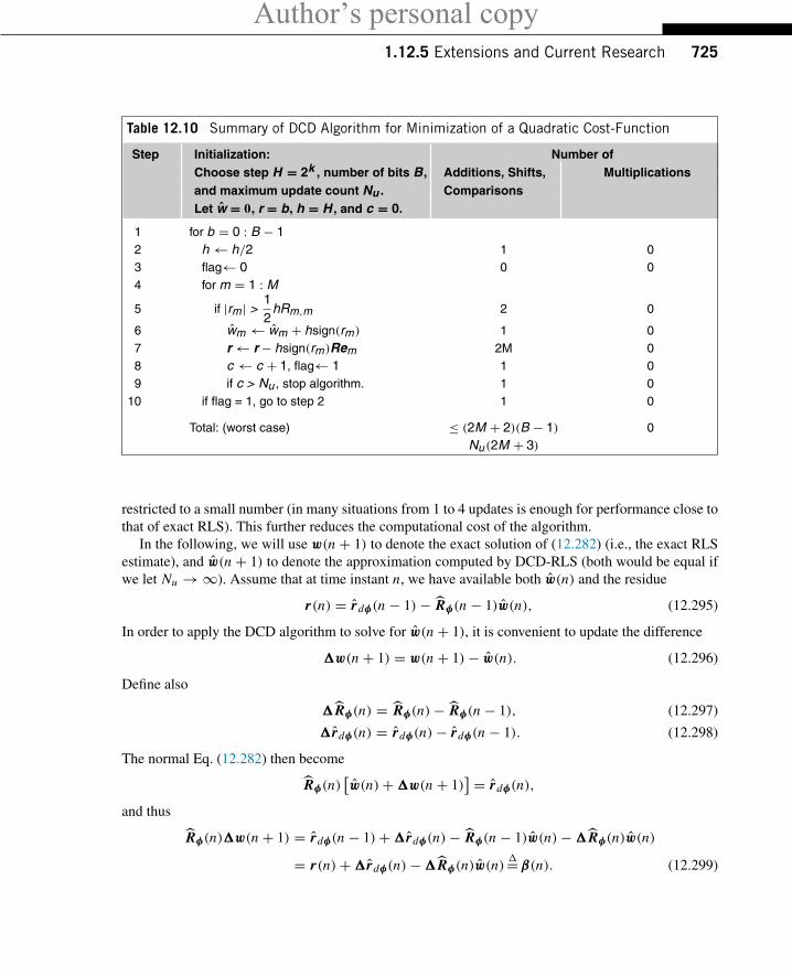
Author’s personal copy1.12.5 Extensions and Current Research 725
Table 12.10 Summary of DCD Algorithm for Minimization of a Quadratic Cost-Function
Step Initialization: Number ofChoose step H = 2k , number of bits B, Additions, Shifts, Multiplicationsand maximum update count Nu . ComparisonsLet w = 0, r = b, h = H , and c = 0.
1 for b = 0 : B − 12 h← h/2 1 03 flag← 0 0 04 for m = 1 : M5 if |rm | > 1
2hRm,m 2 0
6 wm ← wm + hsign(rm) 1 07 r← r− hsign(rm)Rem 2M 08 c ← c + 1, flag← 1 1 09 if c > Nu , stop algorithm. 1 0
10 if flag = 1, go to step 2 1 0
Total: (worst case) ≤ (2M + 2)(B − 1) 0Nu (2M + 3)
restricted to a small number (in many situations from 1 to 4 updates is enough for performance close tothat of exact RLS). This further reduces the computational cost of the algorithm.
In the following, we will use w(n + 1) to denote the exact solution of (12.282) (i.e., the exact RLSestimate), and w(n + 1) to denote the approximation computed by DCD-RLS (both would be equal ifwe let Nu →∞). Assume that at time instant n, we have available both w(n) and the residue
r(n) = rdφ(n − 1)− Rφ(n − 1)w(n), (12.295)
In order to apply the DCD algorithm to solve for w(n + 1), it is convenient to update the difference
�w(n + 1) = w(n + 1)− w(n). (12.296)
Define also
�Rφ(n) = Rφ(n)− Rφ(n − 1), (12.297)
�rdφ(n) = rdφ(n)− rdφ(n − 1). (12.298)
The normal Eq. (12.282) then become
Rφ(n)[w(n)+�w(n + 1)
] = rdφ(n),
and thus
Rφ(n)�w(n + 1) = rdφ(n − 1)+�rdφ(n)− Rφ(n − 1)w(n)−�Rφ(n)w(n)
= r(n)+�rdφ(n)−�Rφ(n)w(n)�=β(n). (12.299)
Author’s personal copy726 CHAPTER 12 Adaptive Filters
Given an approximate solution �w(n+1) to these equations, we obtain an updated approximate solutionw(n + 1) = w(n)+�w(n + 1). Note that the residue of solving (12.282) using w(n + 1),
r(n + 1) = rdφ(n)− Rφ(n)w(n + 1)
= rdφ(n − 1)+�rdφ(n)− Rφ(n)[w(n)+�w(n + 1)
]= rdφ(n − 1)+�rdφ(n)− Rφ(n)�w(n + 1)− [
Rφ(n − 1)+�Rφ(n)]w(n)
= r(n)+�rdφ(n)− Rφ(n)�w(n + 1)−�Rφ(n)w(n)
= β(n)− Rφ(n)�w(n + 1), (12.300)
is exactly the residue of approximately solving (12.299) by �w(n + 1).To complete, we only need to evaluate �Rφ(n) and �rdφ(n). From (12.297), (12.298), (12.283)
and (12.284), we obtain
�Rφ(n) = (λ− 1)Rφ(n − 1)+ φ(n)φT (n), (12.301)
�rdφ(n) = (λ− 1)ddφ(n − 1)+ d(n)φ(n). (12.302)
Substituting these results in the definition of β(n), we obtain
β(n) = r(n)+ (λ− 1)rdφ(n − 1)+ d(n)φ(n)−[(λ− 1)Rφ(n − 1)+ φ(n)φT (n)
]w(n)
= r(n)+ (λ− 1)r(n)+ e(n)φ(n) = λr(n)+ e(n)φ(n). (12.303)
We can therefore use the DCD algorithm to compute an approximate solution to (12.299) and updatethe residue defined by (12.300), as described in Table 12.11.
As we mentioned before, the number of operations of the DCD algorithm can be reduced if wemodify the algorithm in Table 12.10 to update only the entries of the weight vector corresponding tothe largest residue entry, as described in Table 12.12.
The total number of operations of DCD-RLS as described in Tables 12.11 and 12.12 is M2 + 4Mmultiplications and M2/2 + 3.5M + (2M + 1)Nu + B additions. Most of these operations are dueto the updating of Rφ in Table 12.11, which is responsible for the terms in M2. While this cannot behelped for general regressors φ(n), the operation count can be substantially reduced when our filter ismodeling an FIR relation as in (12.41) (i.e., φ(n) is a tap-delay line), as we show next.
If
φ(n) = [x(n) x(n − 1) . . . x(n − M + 1)
]T, (12.304)
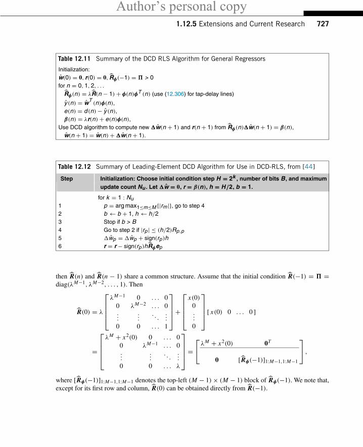
Author’s personal copy1.12.5 Extensions and Current Research 727
Table 12.11 Summary of the DCD RLS Algorithm for General Regressors
Initialization:w(0) = 0, r(0) = 0, Rφ(−1) = � > 0for n = 0, 1, 2, . . .
Rφ(n) = λR(n − 1)+ φ(n)φT (n) (use (12.306) for tap-delay lines)
y (n) = wT(n)φ(n),
e(n) = d (n)− y (n),β(n) = λr(n)+ e(n)φ(n),
Use DCD algorithm to compute new �w(n + 1) and r(n + 1) from Rφ(n)�w(n + 1) = β(n),w(n + 1) = w(n)+�w(n + 1).
Table 12.12 Summary of Leading-Element DCD Algorithm for Use in DCD-RLS, from [44]
Step Initialization: Choose initial condition step H = 2k , number of bits B, and maximumupdate count Nu . Let �w = 0, r = β(n), h = H/2, b = 1.
for k = 1 : Nu1 p = arg max1≤m≤M {|rm |}, go to step 42 b ← b + 1, h← h/23 Stop if b > B4 Go to step 2 if |rp | ≤ (h/2)Rp,p5 �wp = �wp + sign(rp)h6 r = r− sign(rp)hRφep
then R(n) and R(n − 1) share a common structure. Assume that the initial condition R(−1) = � =diag(λM−1, λM−2, . . . , 1). Then
R(0) = λ
⎡⎢⎢⎢⎣λM−1 0 . . . 0
0 λM−2 . . . 0...
.... . .
...
0 0 . . . 1
⎤⎥⎥⎥⎦+⎡⎢⎢⎢⎣
x(0)0...
0
⎤⎥⎥⎥⎦ [ x(0) 0 . . . 0 ]
=
⎡⎢⎢⎢⎣λM + x2(0) 0 . . . 0
0 λM−1 . . . 0...
.... . .
...
0 0 . . . λ
⎤⎥⎥⎥⎦ =⎡⎣λM + x2(0) 0T
0 [Rφ(−1)]1:M−1,1:M−1
⎤⎦ ,where [Rφ(−1)]1:M−1,1:M−1 denotes the top-left (M − 1)× (M − 1) block of Rφ(−1). We note that,except for its first row and column, R(0) can be obtained directly from R(−1).
Author’s personal copy728 CHAPTER 12 Adaptive Filters
Following this observation, we claim that for tapped-delay line regressors, the computation of Rφ(n)in Table 12.11 can be replaced by an update of only its first column [Rφ(n)]1, that is,
[Rφ(n)]1 = λ[Rφ(n − 1)]1 + x(n)φ(n). (12.305)
Since Rφ(n) is symmetric, its first row is the transpose of (12.306), and does not need to be evaluatedagain.
We show next by induction that this pattern holds for all n. We just showed that it it true for n = 0.Assume then that for a certain n, it holds that
Rφ(n) =⎡⎣ (·)Tλ[Rφ(n − 1)]1 + x(n)φ(n)
[Rφ(n − 1)]1:M−1,1:M−1
⎤⎦ , (12.306)
where we use (·)T to indicate that the entries of the first row are the same as the entries of the firstcolumn. We show next that Rφ(n + 1) must follow the same pattern. Indeed,
Rφ(n + 1) = λRφ(n)+
⎡⎢⎢⎢⎣x(n + 1)
x(n)...
n(n − M + 2)
⎤⎥⎥⎥⎦[x(n + 1) x(n) . . . x(n − M + 2)
]
=⎡⎣ (·)Tλ[Rφ(n)]1
λ[Rφ(n − 1)]1:M−1,1:M−1
⎤⎦
+
⎡⎢⎢⎢⎢⎢⎣(·)T
x(n + 1)φ(n + 1) ⎡⎢⎣ x2(n) . . . x(n)x(n − M + 2)...
. . ....
x(n)x(n − M + 2) . . . x2(n − m + 2)
⎤⎥⎦
⎤⎥⎥⎥⎥⎥⎦=⎡⎣ (·)Tλ[Rφ(n)]1 + x(n + 1)φ(n + 1)
[Rφ(n)]1:M−1,1:M−1
⎤⎦ ,where in the last step we identified the (2, 2) block of the intermediate result with the first M − 1 rowsand columns of Rφ(n), from (12.283).
Note that in practice we should not actually move the entries of Rφ(n−1) to their new position; rather,we should use an indexing system to access the entries of Rφ(n) to avoid this costly moving operation.The total number of operations of DCD-RLS using (12.306) is 3M multiplications and 2M Nu + 6Madditions. This is not much larger than the complexity of NLMS. The DCD-RLS algorithm has beenimplemented in FPGAs and run for long periods of time without observation of divergence [44].
Figure 12.35 shows a comparison of RLS and DCD-RLS in a system identification problem. We aretrying to identify an M = 10 FIR filter, so we use (12.306) to update Rφ(n) with lower cost. The input
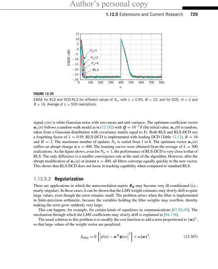
Author’s personal copy1.12.5 Extensions and Current Research 729
100 200 400 500 700 800−30
−25
−20
−15
−10
−5
15
10
5
0
0
EM
SE (
dB)
Nu=4
Nu=2
Nu=1
RLS
n300 600
FIGURE 12.35
EMSE for RLS and DCD-RLS for different values of Nu , with λ = 0.95, M = 10, and for DCD, H = 2 andB = 16. Average of L = 500 realizations.
signal x(n) is white Gaussian noise with zero mean and unit variance. The optimum coefficient vectorwo(n) follows a random-walk model as in (12.182) with Q = 10−5 I (the initial value, wo(0) is random,taken from a Gaussian distribution with covariance matrix equal to I). Both RLS and RLS-DCD usea forgetting factor of λ = 0.95. RLS-DCD is implemented with leading DCD (Table 12.12), B = 16and H = 2. The maximum number of updates Nu is varied from 1 to 8. The optimum vector wo(n)suffers an abrupt change at n = 400. The learning curves were obtained from the average of L = 500realizations. As the figure shows, even for Nu = 1, the performance of RLS-DCD is very close to that ofRLS. The only difference is a smaller convergence rate at the start of the algorithm. However, after theabrupt modification of wo(n) at instant n = 400, all filters converge equally quickly to the new vector.This shows that RLS-DCD does not loose in tracking capability when compared to standard RLS.
1.12.5.2 RegularizationThere are applications in which the autocorrelation matrix Rφ may become very ill-conditioned (i.e.,nearly singular). In these cases, it can be shown that the LMS weight estimates may slowly drift to quitelarge values, even though the error remains small. The problem arises when the filter is implementedin finite-precision arithmetic, because the variables holding the filter weights may overflow, therebymaking the error grow suddenly very large.
This can happen, for example, for certain kinds of equalizers in communications [87,92,93]. Themechanism through which the LMS coefficients may slowly drift is explained in [94,136].
The usual solution to this problem is to modify the cost function to add a term proportional to ‖w‖2,so that large values of the weight vector are penalized:
Jleaky = E
{∣∣∣d(n)− wH φ(n)∣∣∣2}+ α‖w‖2, (12.307)
Author’s personal copy730 CHAPTER 12 Adaptive Filters
where ‖·‖ is the Euclidean norm andα > 0 is a small constant. With this cost function, the correspondingalgorithm is
w(n + 1) = (1− μα)w(n)+ μe∗(n)φ(n). (12.308)
This is known as leaky-LMS algorithm [4]. It can be shown that the introduction of leakage will bias thesolution away from the Wiener solution, but will prevent any excessive growth of the weight coefficients.A detailed analysis of the leaky-LMS algorithm is available in [137]. Reference [94] proposes a modifiedversion of the algorithm without the bias.
Difficulties with singular or near-singular autocorrelation matrices also appears with RLS. For exam-ple, if the input is a periodic signal with little noise, the autocorrelation matrix will become nearlysingular, and matrix P(n) in RLS will diverge. This problem, as well as a solution to it using variableforgetting-factor, is described in [138]. A constant regularization method based on DCD can be foundin [139]. Another approach, valid only for short filters, but which allows constant regularization, isdescribed in [140].
The leaky-LMS algorithm has found other important applications, most particularly in beamforming,in which it is used to turn the beamformer robust against array imperfections [141]. The algorithms usedin beamforming are examples of constrained adaptive filters, in which the cost function incorporatesequality conditions that must be satisfied at all times—see Section 1.12.5.11.
Another algorithm closely related to leaky-LMS, in which the extra term in the cost function penal-izes large values of the filter output (that is, α|wH (n)φ(n)|2 instead of α‖w(n)‖2 in (12.307)), wasrecently employed to improve the performance of FIR adaptive filters in the presence of saturationnonlinearities [142].
More recent applications of regularization involve the use of the �1-norm,
‖w‖1 = |w0| + |w1| + . . .+ |wM−1|,instead of the Euclidean norm. This is because the �1 norm promotes solutions that are sparse, that is,a filter that minimizes the cost function
Jsparse = E
{∣∣∣d(n)− wH φ(n)∣∣∣2}+ α‖w‖1, (12.309)
will favor solutions in which the vector w has only a few nonzero entries (an intuitive explanationfor this can be found in [143], which is a good introduction to compressive sensing). Algorithms forpromoting sparsity have been receiving much attention lately, due to the interest in compressive sensingapplications [144–148]. See also the references for the proportionate NLMS (PNLMS) algorithm inSection 1.12.5.3.
1.12.5.3 Variable step-sizeThe steady-state analysis of Section 1.12.4.4 shows that the step-sizeμplays an import role in controllingthe performance of the LMS algorithm since it is one of the main factors affecting the convergence rateand the misadjustment. To obtain a better tradeoff between convergence speed and steady-sate EMSE,several authors proposed different forms of adjusting the step-size of LMS. Variable step-size algorithmsallow the filters to dynamically adjust their performance in response to conditions in the input data anderror signals.
Author’s personal copy1.12.5 Extensions and Current Research 731
In this context, one of the most popular algorithms is the variable step-size LMS (VSLMS) proposedin [149]. In the VSLMS algorithm, each coefficient wk(n), k = 0, . . . ,M − 1 is updated with a time-varying step-size μk(n), whose adjustment is given by
μk(n) = μk(n − 1)+ ρsign[e(n)φk(n)
]sign[e(n − 1)φk(n − 1)], (12.310)
where ρ is a small positive constant. This algorithm operates in a very intuitive way. When the algorithmhas not yet converged, the gradient term e(n)φk(n) shows a positive or negative direction in successiveiterations and the step-size μk(n) increases up to an allowed maximum value. On the other hand, nearsteady-state e(n)φk(n) approaches zero and its sign changes in successive iterations, which reducesμk(n) (the step-size is lower-bounded by a small minimum value). Therefore, during the initial conver-gence VSLMS uses a large step-size, which leads to a high convergence rate. When its coefficients areclose to the optimum solution, the algorithm is updated with a small step-size, which allows VSLMSto achieve a small EMSE. A variant of this algorithm is obtained by dropping the sign functions in(12.310), i.e.,
μk(n) = μk(n − 1)+ ρe(n)e(n − 1)φk(n)φk(n − 1). (12.311)
The choice between (12.310) and (12.311) depends on the application [150].The NLMS algorithm, proposed independently by Nagumo and Noda [151] and Albert and Gardner
[152], can be interpreted a variable step-size LMS with a particular choice forμ(n) (see Section 1.12.3.2).An important variant of NLMS is the so-called power-normalized LMS (PN-LMS) algorithm, whichuses the following variable step-size
μ(n) = μ
ε + p(n), (12.312)
where
p(n) = γ p(n − 1)+ (1− γ )|φ0(n)|2, (12.313)
with p(−1) = 0 and γ being a positive scalar chosen from within the interval 0 < γ ≤ 1. Thisalgorithm is useful when the regressor is a tapped-delay line, that is, when φi (n) = x(n − i), so thatthe scalar p(n) is an estimate for the power of the input sequence {x(n)}. The range of μ in (12.312) is0 ≤ μ ≤ 2
M [3].Over the years, several variable step-size algorithms were proposed in the literature. Some of these
algorithms are in the papers [153–167] and in their references. Besides the variable step-size approaches,an alternative scheme to improve the tradeoff between convergence speed and steady-sate EMSE isconstituted by combinations of adaptive algorithms, described in Section 1.12.5.8.1.
Another class of variable step-size algorithms was developed specifically to accelerate the conver-gence of filters whose optimum weight vector wo is sparse, that is, has only a small fraction of nonzeroelements. The primary application for this is echo cancellation, mainly for echo due to reflections in thetelephone connection. The algorithms are known as proportionate NLMS (PNLMS) algorithms, andhave usually very good performance for approximating sparse weight vectors [168–172].
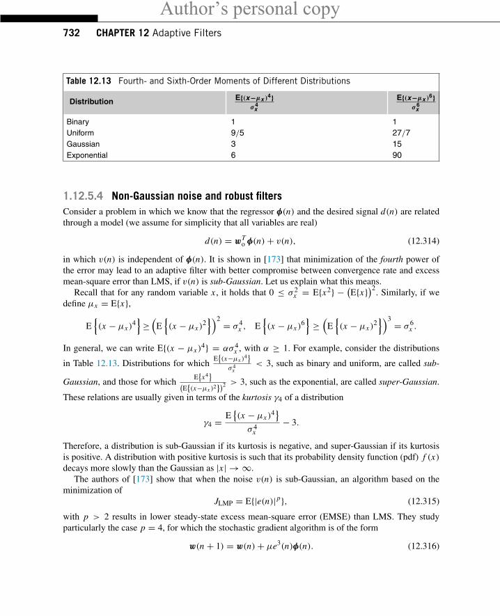
Author’s personal copy732 CHAPTER 12 Adaptive Filters
Table 12.13 Fourth- and Sixth-Order Moments of Different Distributions
Distribution E{(x−μx )4}σ4
x
E{(x−μx )6}σ6
x
Binary 1 1Uniform 9/5 27/7Gaussian 3 15Exponential 6 90
1.12.5.4 Non-Gaussian noise and robust filtersConsider a problem in which we know that the regressor φ(n) and the desired signal d(n) are relatedthrough a model (we assume for simplicity that all variables are real)
d(n) = wTo φ(n)+ v(n), (12.314)
in which v(n) is independent of φ(n). It is shown in [173] that minimization of the fourth power ofthe error may lead to an adaptive filter with better compromise between convergence rate and excessmean-square error than LMS, if v(n) is sub-Gaussian. Let us explain what this means.
Recall that for any random variable x , it holds that 0 ≤ σ 2x = E{x2} − (
E{x})2. Similarly, if wedefine μx = E{x},
E{(x − μx )
4}≥(
E{(x − μx )
2})2 = σ 4
x , E{(x − μx )
6}≥(
E{(x − μx )
2})3 = σ 6
x .
In general, we can write E{(x − μx )4} = ασ 4
x , with α ≥ 1. For example, consider the distributions
in Table 12.13. Distributions for whichE{(x−μx )
4}
σ 4x
< 3, such as binary and uniform, are called sub-
Gaussian, and those for whichE{
x4}(
E{(x−μx )2})2 > 3, such as the exponential, are called super-Gaussian.
These relations are usually given in terms of the kurtosis γ4 of a distribution
γ4 = E{(x − μx )
4}
σ 4x
− 3.
Therefore, a distribution is sub-Gaussian if its kurtosis is negative, and super-Gaussian if its kurtosisis positive. A distribution with positive kurtosis is such that its probability density function (pdf) f (x)decays more slowly than the Gaussian as |x | → ∞.
The authors of [173] show that when the noise v(n) is sub-Gaussian, an algorithm based on theminimization of
JLMP = E{|e(n)|p}, (12.315)
with p > 2 results in lower steady-state excess mean-square error (EMSE) than LMS. They studyparticularly the case p = 4, for which the stochastic gradient algorithm is of the form
w(n + 1) = w(n)+ μe3(n)φ(n). (12.316)
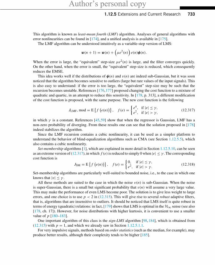
Author’s personal copy1.12.5 Extensions and Current Research 733
This algorithm is known as least-mean fourth (LMF) algorithm. Analyses of general algorithms witherror nonlinearities can be found in [174], and a unified analysis is available in [175].
The LMF algorithm can be understood intuitively as a variable-step version of LMS:
w(n + 1) = w(n)+(μe2(n)
)e(n)φ(n).
When the error is large, the “equivalent” step-size μe2(n) is large, and the filter converges quickly.On the other hand, when the error is small, the “equivalent” step-size is reduced, which consequentlyreduces the EMSE.
This idea works well if the distributions of φ(n) and v(n) are indeed sub-Gaussian, but it was soonnoticed that the algorithm becomes sensitive to outliers (large but rare values of the input signals). Thisis also easy to understand: if the error is too large, the “equivalent” step-size may be such that therecursion becomes unstable. References [176,177] proposed changing the cost function to a mixture ofquadratic and quartic, in an attempt to reduce this sensitivity. In [178, p. 313], a different modificationof the cost function is proposed, with the same purpose. The new cost function is the following
JLMF,mod = E{
f(e(n)
)}, f (e) =
{e4, if |e| ≤ γ,e2, if |e| > γ,
(12.317)
in which γ is a constant. References [45,59] show that when the regressor is Gaussian, LMF has anon-zero probability of diverging. From these results one can see that the solution proposed in [178]indeed stabilizes the algorithm.
Since the LMF recursion contains a cubic nonlinearity, it can be used as a simpler platform tounderstand the behavior of blind-equalization algorithms such as CMA (see Section 1.12.5.5), whichalso contains a cubic nonlinearity.
Set-membership algorithms [1], which are explained in more detail in Section 1.12.5.10, can be seenas an extreme version of (12.317), in which f (e) is reduced to simply 0 when |e| ≤ γ . The correspondingcost function is
JSM = E{
f(e(n)
)}, f (e) =
{0, if |e| ≤ γ,e2, if |e| > γ.
(12.318)
Set-membership algorithms are particularly well-suited to bounded noise, i.e., to the case in which oneknows that |v| ≤ γ .
All these methods are suited to the case in which the noise v(n) is sub-Gaussian. When the noiseis super-Gaussian, there is a small but significant probability that v(n) will assume a very large value.This may make the performance of even LMS become poor. The solution is to give less weight to largeerrors, and one choice is to use p < 2 in (12.315). This will give rise to several robust adaptive filters,that is, algorithms that are insensitive to outliers. It should be noticed that LMS itself is quite robust interms of energy (quadratic) relations: in fact, [179] shows that LMS is optimal in the H∞ sense (see also[178, ch. 17]). However, for noise distributions with higher kurtosis, it is convenient to use a smallervalue of p [180–183].
One important algorithm of this class is the sign-LMS algorithm [98,184], which is obtained from(12.315) with p = 1, and which we already saw in Section 1.12.5.1.1.
For very impulsive signals, methods based on order statistics (such as the median, for example), mayproduce better results, although their complexity tends to be higher [185].
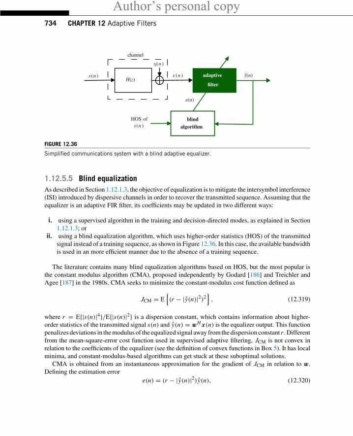
Author’s personal copy734 CHAPTER 12 Adaptive Filters
adaptive
filter
blindalgorithm
HOS ofs (n )
channel
η(n )
e(n)
s (n ) x (n ) y(n)H(z)
ˆ
FIGURE 12.36
Simplified communications system with a blind adaptive equalizer.
1.12.5.5 Blind equalizationAs described in Section 1.12.1.3, the objective of equalization is to mitigate the intersymbol interference(ISI) introduced by dispersive channels in order to recover the transmitted sequence. Assuming that theequalizer is an adaptive FIR filter, its coefficients may be updated in two different ways:
i. using a supervised algorithm in the training and decision-directed modes, as explained in Section1.12.1.3; or
ii. using a blind equalization algorithm, which uses higher-order statistics (HOS) of the transmittedsignal instead of a training sequence, as shown in Figure 12.36. In this case, the available bandwidthis used in an more efficient manner due to the absence of a training sequence.
The literature contains many blind equalization algorithms based on HOS, but the most popular isthe constant modulus algorithm (CMA), proposed independently by Godard [186] and Treichler andAgee [187] in the 1980s. CMA seeks to minimize the constant-modulus cost function defined as
JCM = E{(r − |y(n)|2)2
}, (12.319)
where r = E{|s(n)|4}/E{|s(n)|2} is a dispersion constant, which contains information about higher-order statistics of the transmitted signal s(n) and y(n) = wH x(n) is the equalizer output. This functionpenalizes deviations in the modulus of the equalized signal away from the dispersion constant r . Differentfrom the mean-square-error cost function used in supervised adaptive filtering, JCM is not convex inrelation to the coefficients of the equalizer (see the definition of convex functions in Box 5). It has localminima, and constant-modulus-based algorithms can get stuck at these suboptimal solutions.
CMA is obtained from an instantaneous approximation for the gradient of JCM in relation to w.Defining the estimation error
e(n) = (r − |y(n)|2)y(n), (12.320)
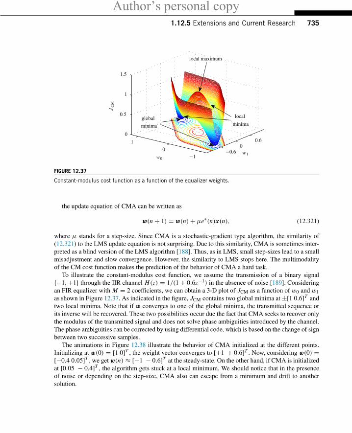
Author’s personal copy1.12.5 Extensions and Current Research 735
0
00
0.6
0.5
−0.6
1
1
1.5
−1
global local
minima minima
local maximum
JC
M
w0w1
FIGURE 12.37
Constant-modulus cost function as a function of the equalizer weights.
the update equation of CMA can be written as
w(n + 1) = w(n)+ μe∗(n)x(n), (12.321)
where μ stands for a step-size. Since CMA is a stochastic-gradient type algorithm, the similarity of(12.321) to the LMS update equation is not surprising. Due to this similarity, CMA is sometimes inter-preted as a blind version of the LMS algorithm [188]. Thus, as in LMS, small step-sizes lead to a smallmisadjustment and slow convergence. However, the similarity to LMS stops here. The multimodalityof the CM cost function makes the prediction of the behavior of CMA a hard task.
To illustrate the constant-modulus cost function, we assume the transmission of a binary signal{−1,+1} through the IIR channel H(z) = 1/(1+ 0.6z−1) in the absence of noise [189]. Consideringan FIR equalizer with M = 2 coefficients, we can obtain a 3-D plot of JCM as a function of w0 and w1as shown in Figure 12.37. As indicated in the figure, JCM contains two global minima at±[1 0.6]T andtwo local minima. Note that if w converges to one of the global minima, the transmitted sequence orits inverse will be recovered. These two possibilities occur due the fact that CMA seeks to recover onlythe modulus of the transmitted signal and does not solve phase ambiguities introduced by the channel.The phase ambiguities can be corrected by using differential code, which is based on the change of signbetween two successive samples.
The animations in Figure 12.38 illustrate the behavior of CMA initialized at the different points.Initializing at w(0) = [1 0]T , the weight vector converges to [+1 + 0.6]T . Now, considering w(0) =[−0.4 0.05]T , we get w(n) ≈ [−1 − 0.6]T at the steady-state. On the other hand, if CMA is initializedat [0.05 − 0.4]T , the algorithm gets stuck at a local minimum. We should notice that in the presenceof noise or depending on the step-size, CMA also can escape from a minimum and drift to anothersolution.
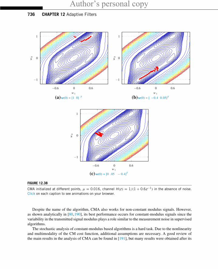
Author’s personal copy736 CHAPTER 12 Adaptive Filters
0
0 0.6−0.6
1
−1
w0
w 1
(a)w(0) = [1 0] T
0
0 0.6−0.6
1
−1
w0
w 1
(b)w(0) = [ −0.4 0.05]T
0
0 0.6−0.6
1
−1
w0
w 1
(c)w(0) = [0 .05 − 0.4]T
FIGURE 12.38
CMA initialized at different points, μ = 0.016, channel H(z ) = 1/(1 + 0.6z−1) in the absence of noise.Click on each caption to see animations on your browser.
Despite the name of the algorithm, CMA also works for non-constant modulus signals. However,as shown analytically in [80,190], its best performance occurs for constant-modulus signals since thevariability in the transmitted signal modulus plays a role similar to the measurement noise in supervisedalgorithms.
The stochastic analysis of constant-modulus based algorithms is a hard task. Due to the nonlinearityand multimodality of the CM cost function, additional assumptions are necessary. A good review ofthe main results in the analysis of CMA can be found in [191], but many results were obtained after its
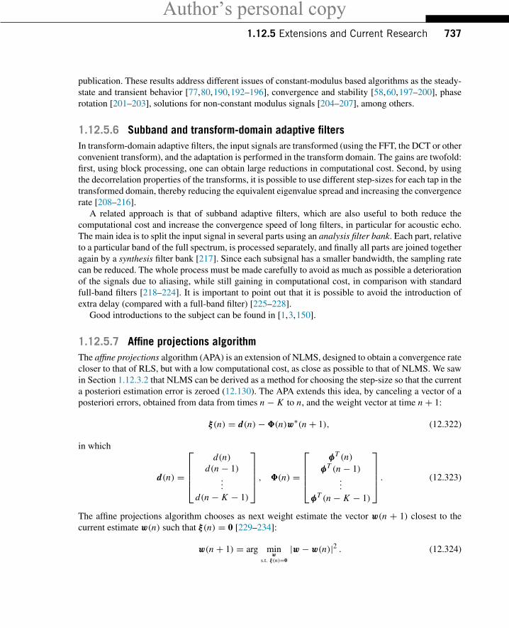
Author’s personal copy1.12.5 Extensions and Current Research 737
publication. These results address different issues of constant-modulus based algorithms as the steady-state and transient behavior [77,80,190,192–196], convergence and stability [58,60,197–200], phaserotation [201–203], solutions for non-constant modulus signals [204–207], among others.
1.12.5.6 Subband and transform-domain adaptive filtersIn transform-domain adaptive filters, the input signals are transformed (using the FFT, the DCT or otherconvenient transform), and the adaptation is performed in the transform domain. The gains are twofold:first, using block processing, one can obtain large reductions in computational cost. Second, by usingthe decorrelation properties of the transforms, it is possible to use different step-sizes for each tap in thetransformed domain, thereby reducing the equivalent eigenvalue spread and increasing the convergencerate [208–216].
A related approach is that of subband adaptive filters, which are also useful to both reduce thecomputational cost and increase the convergence speed of long filters, in particular for acoustic echo.The main idea is to split the input signal in several parts using an analysis filter bank. Each part, relativeto a particular band of the full spectrum, is processed separately, and finally all parts are joined togetheragain by a synthesis filter bank [217]. Since each subsignal has a smaller bandwidth, the sampling ratecan be reduced. The whole process must be made carefully to avoid as much as possible a deteriorationof the signals due to aliasing, while still gaining in computational cost, in comparison with standardfull-band filters [218–224]. It is important to point out that it is possible to avoid the introduction ofextra delay (compared with a full-band filter) [225–228].
Good introductions to the subject can be found in [1,3,150].
1.12.5.7 Affine projections algorithmThe affine projections algorithm (APA) is an extension of NLMS, designed to obtain a convergence ratecloser to that of RLS, but with a low computational cost, as close as possible to that of NLMS. We sawin Section 1.12.3.2 that NLMS can be derived as a method for choosing the step-size so that the currenta posteriori estimation error is zeroed (12.130). The APA extends this idea, by canceling a vector of aposteriori errors, obtained from data from times n − K to n, and the weight vector at time n + 1:
ξ(n) = d(n)−�(n)w∗(n + 1), (12.322)
in which
d(n) =
⎡⎢⎢⎢⎣d(n)
d(n − 1)...
d(n − K − 1)
⎤⎥⎥⎥⎦ , �(n) =
⎡⎢⎢⎢⎣φT (n)
φT (n − 1)...
φT (n − K − 1)
⎤⎥⎥⎥⎦ . (12.323)
The affine projections algorithm chooses as next weight estimate the vector w(n + 1) closest to thecurrent estimate w(n) such that ξ(n) = 0 [229–234]:
w(n + 1) = arg minw
s.t. ξ(n)=0
|w − w(n)|2 . (12.324)
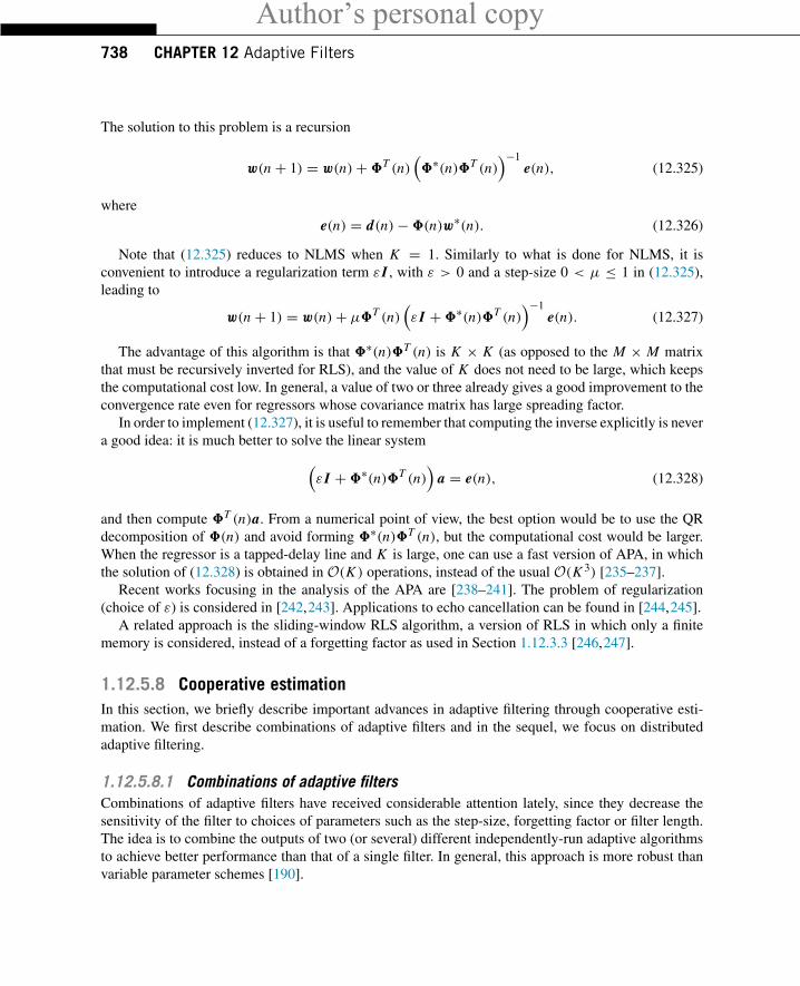
Author’s personal copy738 CHAPTER 12 Adaptive Filters
The solution to this problem is a recursion
w(n + 1) = w(n)+�T (n)(�∗(n)�T (n)
)−1e(n), (12.325)
wheree(n) = d(n)−�(n)w∗(n). (12.326)
Note that (12.325) reduces to NLMS when K = 1. Similarly to what is done for NLMS, it isconvenient to introduce a regularization term ε I , with ε > 0 and a step-size 0 < μ ≤ 1 in (12.325),leading to
w(n + 1) = w(n)+ μ�T (n)(ε I +�∗(n)�T (n)
)−1e(n). (12.327)
The advantage of this algorithm is that �∗(n)�T (n) is K × K (as opposed to the M × M matrixthat must be recursively inverted for RLS), and the value of K does not need to be large, which keepsthe computational cost low. In general, a value of two or three already gives a good improvement to theconvergence rate even for regressors whose covariance matrix has large spreading factor.
In order to implement (12.327), it is useful to remember that computing the inverse explicitly is nevera good idea: it is much better to solve the linear system(
ε I +�∗(n)�T (n))
a = e(n), (12.328)
and then compute �T (n)a. From a numerical point of view, the best option would be to use the QRdecomposition of �(n) and avoid forming �∗(n)�T (n), but the computational cost would be larger.When the regressor is a tapped-delay line and K is large, one can use a fast version of APA, in whichthe solution of (12.328) is obtained in O(K ) operations, instead of the usual O(K 3) [235–237].
Recent works focusing in the analysis of the APA are [238–241]. The problem of regularization(choice of ε) is considered in [242,243]. Applications to echo cancellation can be found in [244,245].
A related approach is the sliding-window RLS algorithm, a version of RLS in which only a finitememory is considered, instead of a forgetting factor as used in Section 1.12.3.3 [246,247].
1.12.5.8 Cooperative estimationIn this section, we briefly describe important advances in adaptive filtering through cooperative esti-mation. We first describe combinations of adaptive filters and in the sequel, we focus on distributedadaptive filtering.
1.12.5.8.1 Combinations of adaptive filtersCombinations of adaptive filters have received considerable attention lately, since they decrease thesensitivity of the filter to choices of parameters such as the step-size, forgetting factor or filter length.The idea is to combine the outputs of two (or several) different independently-run adaptive algorithmsto achieve better performance than that of a single filter. In general, this approach is more robust thanvariable parameter schemes [190].
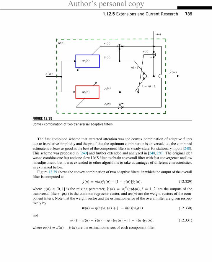
Author’s personal copy1.12.5 Extensions and Current Research 739
φ ( n )
d(n)
e(n)
e1(n)
e2(n)
y1(n)
y2(n)
y ( n )
η ( n )
1 − η ( n )
w1(n)
w2(n)
w(n)
FIGURE 12.39
Convex combination of two transversal adaptive filters.
The first combined scheme that attracted attention was the convex combination of adaptive filtersdue to its relative simplicity and the proof that the optimum combination is universal, i.e., the combinedestimate is at least as good as the best of the component filters in steady-state, for stationary inputs [248].This scheme was proposed in [249] and further extended and analyzed in [248,250]. The original ideawas to combine one fast and one slow LMS filter to obtain an overall filter with fast convergence and lowmisadjustment, but it was extended to other algorithms to take advantages of different characteristics,as explained below.
Figure 12.39 shows the convex combination of two adaptive filters, in which the output of the overallfilter is computed as
y(n) = η(n)y1(n)+ [1− η(n)]y2(n), (12.329)
where η(n) ∈ [0, 1] is the mixing parameter, yi (n) = wHi (n)φ(n), i = 1, 2, are the outputs of the
transversal filters, φ(n) is the common regressor vector, and wi (n) are the weight vectors of the com-ponent filters. Note that the weight vector and the estimation error of the overall filter are given respec-tively by
w(n) = η(n)w1(n)+ [1− η(n)]w2(n) (12.330)
ande(n) = d(n)− y(n) = η(n)e1(n)+ [1− η(n)]e2(n), (12.331)
where ei (n) = d(n)− yi (n) are the estimation errors of each component filter.
Author’s personal copy740 CHAPTER 12 Adaptive Filters
In order to restrict the mixing parameter to the interval [0, 1] and to reduce gradient noise whenη(n) ≈ 0 or η(n) ≈ 1, a nonlinear transformation and an auxiliary variable a(n) are used, i.e.,
η(n) = sgm[a(n)] � 1
1+ e−a(n), (12.332)
where a(n) is updated to minimize the overall squared error e2(n), i.e.,
a(n + 1) = a(n)− μa
2∇ae2(n) = a(n)+ μa
[y1(n)− y2(n)
]e(n)η(n)
[1− η(n)] . (12.333)
In practice, a(n)must be restricted by saturation of (12.333) to an interval [−a+, a+], since the factorη(n)
[1− η(n)] would virtually stop adaptation if a(n) were allowed to grow too much. The correct
adjustment of the step-size μa depends on the input signal and additive noise powers and also on thestep-sizes of the component filters. To make the choice of μa independent of the filtering scenario, anormalized scheme was proposed in [251].
The combination of one fast and one slow LMS (with μ1 > μ2) operates in a very intuitive way.When fast changes appear, the fast filter outperforms the slow one, making η(n) ≈ 1. In stationarysituations, the slow filter gets a lower quadratic error and η(n) ≈ 0, which allows the overall filterto achieve the misadjustment of the slow LMS filter. There are situations in which the combinationoutperforms each component filter and in these cases, 0 < η(n) < 1. This behavior can be observed inthe simulation results shown in Figure 12.40, where the convex combination of two LMS filters withdifferent step-sizes (μ1 = 0.1 and μ2 = 0.01) was used to identity the system (from [248])[
0.9003 −0.5377 0.2137 −0.0280 0.7826 0.5242 −0.0871].
The regressor φ(n) is obtained from a process x(n) generated with a first-order autoregressive model,whose transfer function is
√1− b2/(1−bz−1). This model is fed with an iid Gaussian random process,
whose variance is such that Tr(Rφ) = 1. Moreover, additive iid noise v(n) with variance σ 2v = 0.01 is
added to form the desired signal. Figure 12.40a shows the EMSE curves estimated from the ensemble-average of 500 independent runs and filtered by a moving-average filter with 128 coefficients to facil-itate the visualization. The combined filter acquires the faster convergence of μ1-LMS and attains theEMSE of μ2-LMS. Figure 12.40b shows the time evolution of the mixing parameter. We can observethat it rapidly changes toward sgm[a+] during the initial convergence, while its steady-state value is1− sgm[a+].
After the publication of [249], many papers on combinations of adaptive filters appeared in theliterature. Apparently, the idea of combining the outputs of several different independently-run adaptivealgorithms was first proposed in [252], and later improved in [253,254]. The algorithms proposedin [252–254] are based on a Bayesian argument, and construct an overall (combined) filter through alinear combination of the outputs of several independent adaptive filters. The weights are the a posterioriprobabilities that the underlying models used to describe each individual algorithm are “true.” Since theweights add up to one, in a sense these first papers also proposed “convex” combinations of algorithms.Unconstrained linear combinations of adaptive filters were also proposed in [255]. However, the methodof [248,249] has received more attention due to its relative simplicity and the proof that the optimumcombination is universal. By this, we mean that if the combination uses at every instant the optimum

Author’s personal copy1.12.5 Extensions and Current Research 741
combination
µ2-LMSµ1-LMS
EM
SE(d
B)
(a)
0
0 1 2 3
−10
−20
−30
−40
−50
E{η
(n) }
(b)
00
1
1
0.5
× 104
2 3
iterations
FIGURE 12.40
(a) EMSE for μ1-LMS, μ2-LMS, and their convex combination; (b) ensemble-average of η(n);μ1 = 0.1, μ2 =0.01, μa = 100, a+ = 4, b = 0.8; mean of 500 independent runs.
value of η, then the combined filter is always at least as good as the best component filter. However, inpractice η must also be estimated, so the performance of the combination may be slightly worse thanthat of the best filter.
In the sequel, we briefly describe some of the most important recent contributions in this area.In [250], the convergence of the overall filter is greatly improved by transferring a part of the fast
filter w1 to the slow filter w2 when λ(n) ≥ γ , that is,
w2(n + 1) = α [w2(n)+ μ2e2(n)x(n)]+ (1− α)w1(n), (12.334)
where α is a parameter close to 1 and γ is a threshold close to the maximum value that can be reachedby λ(n).
A steady-state analysis of the combined filter was presented in [248]. This analysis shows that theconvex combination is universal if the optimum η is used, a property that was exploited to design filters
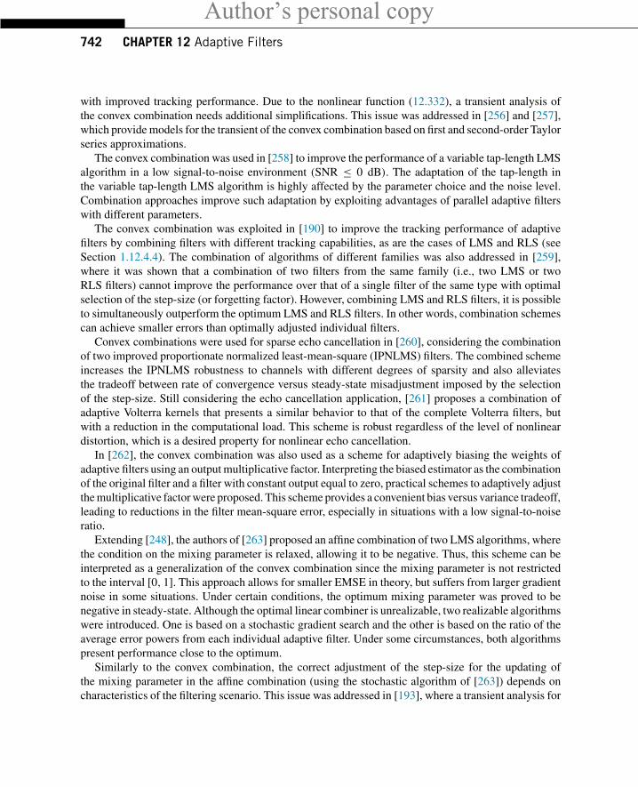
Author’s personal copy742 CHAPTER 12 Adaptive Filters
with improved tracking performance. Due to the nonlinear function (12.332), a transient analysis ofthe convex combination needs additional simplifications. This issue was addressed in [256] and [257],which provide models for the transient of the convex combination based on first and second-order Taylorseries approximations.
The convex combination was used in [258] to improve the performance of a variable tap-length LMSalgorithm in a low signal-to-noise environment (SNR ≤ 0 dB). The adaptation of the tap-length inthe variable tap-length LMS algorithm is highly affected by the parameter choice and the noise level.Combination approaches improve such adaptation by exploiting advantages of parallel adaptive filterswith different parameters.
The convex combination was exploited in [190] to improve the tracking performance of adaptivefilters by combining filters with different tracking capabilities, as are the cases of LMS and RLS (seeSection 1.12.4.4). The combination of algorithms of different families was also addressed in [259],where it was shown that a combination of two filters from the same family (i.e., two LMS or twoRLS filters) cannot improve the performance over that of a single filter of the same type with optimalselection of the step-size (or forgetting factor). However, combining LMS and RLS filters, it is possibleto simultaneously outperform the optimum LMS and RLS filters. In other words, combination schemescan achieve smaller errors than optimally adjusted individual filters.
Convex combinations were used for sparse echo cancellation in [260], considering the combinationof two improved proportionate normalized least-mean-square (IPNLMS) filters. The combined schemeincreases the IPNLMS robustness to channels with different degrees of sparsity and also alleviatesthe tradeoff between rate of convergence versus steady-state misadjustment imposed by the selectionof the step-size. Still considering the echo cancellation application, [261] proposes a combination ofadaptive Volterra kernels that presents a similar behavior to that of the complete Volterra filters, butwith a reduction in the computational load. This scheme is robust regardless of the level of nonlineardistortion, which is a desired property for nonlinear echo cancellation.
In [262], the convex combination was also used as a scheme for adaptively biasing the weights ofadaptive filters using an output multiplicative factor. Interpreting the biased estimator as the combinationof the original filter and a filter with constant output equal to zero, practical schemes to adaptively adjustthe multiplicative factor were proposed. This scheme provides a convenient bias versus variance tradeoff,leading to reductions in the filter mean-square error, especially in situations with a low signal-to-noiseratio.
Extending [248], the authors of [263] proposed an affine combination of two LMS algorithms, wherethe condition on the mixing parameter is relaxed, allowing it to be negative. Thus, this scheme can beinterpreted as a generalization of the convex combination since the mixing parameter is not restrictedto the interval [0, 1]. This approach allows for smaller EMSE in theory, but suffers from larger gradientnoise in some situations. Under certain conditions, the optimum mixing parameter was proved to benegative in steady-state. Although the optimal linear combiner is unrealizable, two realizable algorithmswere introduced. One is based on a stochastic gradient search and the other is based on the ratio of theaverage error powers from each individual adaptive filter. Under some circumstances, both algorithmspresent performance close to the optimum.
Similarly to the convex combination, the correct adjustment of the step-size for the updating ofthe mixing parameter in the affine combination (using the stochastic algorithm of [263]) depends oncharacteristics of the filtering scenario. This issue was addressed in [193], where a transient analysis for
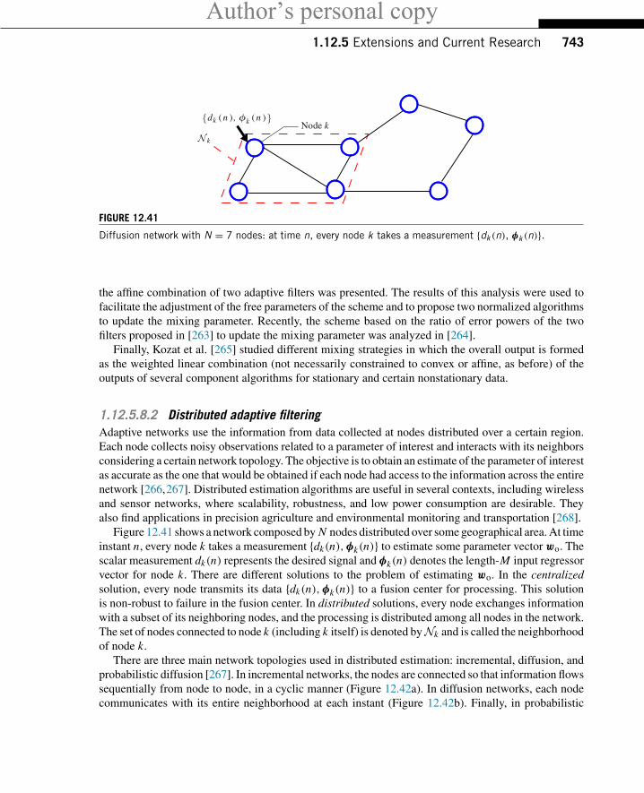
Author’s personal copy1.12.5 Extensions and Current Research 743
N k
Node k{dk ( n ) , φk ( n )}
FIGURE 12.41
Diffusion network with N = 7 nodes: at time n, every node k takes a measurement {dk (n), φk (n)}.
the affine combination of two adaptive filters was presented. The results of this analysis were used tofacilitate the adjustment of the free parameters of the scheme and to propose two normalized algorithmsto update the mixing parameter. Recently, the scheme based on the ratio of error powers of the twofilters proposed in [263] to update the mixing parameter was analyzed in [264].
Finally, Kozat et al. [265] studied different mixing strategies in which the overall output is formedas the weighted linear combination (not necessarily constrained to convex or affine, as before) of theoutputs of several component algorithms for stationary and certain nonstationary data.
1.12.5.8.2 Distributed adaptive filteringAdaptive networks use the information from data collected at nodes distributed over a certain region.Each node collects noisy observations related to a parameter of interest and interacts with its neighborsconsidering a certain network topology. The objective is to obtain an estimate of the parameter of interestas accurate as the one that would be obtained if each node had access to the information across the entirenetwork [266,267]. Distributed estimation algorithms are useful in several contexts, including wirelessand sensor networks, where scalability, robustness, and low power consumption are desirable. Theyalso find applications in precision agriculture and environmental monitoring and transportation [268].
Figure 12.41 shows a network composed by N nodes distributed over some geographical area. At timeinstant n, every node k takes a measurement {dk(n),φk(n)} to estimate some parameter vector wo. Thescalar measurement dk(n) represents the desired signal and φk(n) denotes the length-M input regressorvector for node k. There are different solutions to the problem of estimating wo. In the centralizedsolution, every node transmits its data {dk(n),φk(n)} to a fusion center for processing. This solutionis non-robust to failure in the fusion center. In distributed solutions, every node exchanges informationwith a subset of its neighboring nodes, and the processing is distributed among all nodes in the network.The set of nodes connected to node k (including k itself) is denoted by Nk and is called the neighborhoodof node k.
There are three main network topologies used in distributed estimation: incremental, diffusion, andprobabilistic diffusion [267]. In incremental networks, the nodes are connected so that information flowssequentially from node to node, in a cyclic manner (Figure 12.42a). In diffusion networks, each nodecommunicates with its entire neighborhood at each instant (Figure 12.42b). Finally, in probabilistic
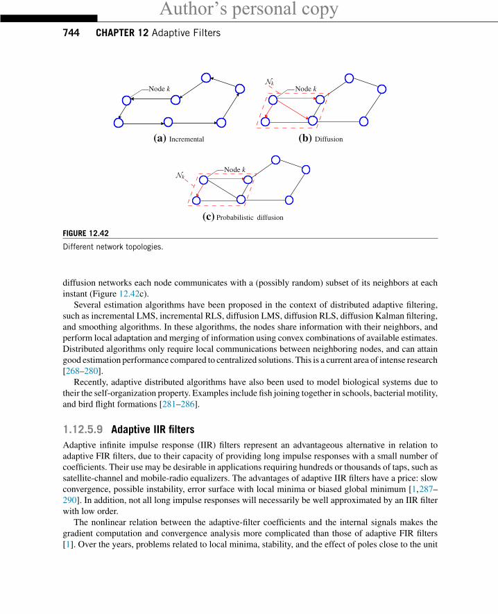
Author’s personal copy744 CHAPTER 12 Adaptive Filters
Node k
(a) Incremental
NkNode k
(b) Diffusion
NkNode k
(c) Probabilistic diffusion
FIGURE 12.42
Different network topologies.
diffusion networks each node communicates with a (possibly random) subset of its neighbors at eachinstant (Figure 12.42c).
Several estimation algorithms have been proposed in the context of distributed adaptive filtering,such as incremental LMS, incremental RLS, diffusion LMS, diffusion RLS, diffusion Kalman filtering,and smoothing algorithms. In these algorithms, the nodes share information with their neighbors, andperform local adaptation and merging of information using convex combinations of available estimates.Distributed algorithms only require local communications between neighboring nodes, and can attaingood estimation performance compared to centralized solutions. This is a current area of intense research[268–280].
Recently, adaptive distributed algorithms have also been used to model biological systems due totheir the self-organization property. Examples include fish joining together in schools, bacterial motility,and bird flight formations [281–286].
1.12.5.9 Adaptive IIR filtersAdaptive infinite impulse response (IIR) filters represent an advantageous alternative in relation toadaptive FIR filters, due to their capacity of providing long impulse responses with a small number ofcoefficients. Their use may be desirable in applications requiring hundreds or thousands of taps, such assatellite-channel and mobile-radio equalizers. The advantages of adaptive IIR filters have a price: slowconvergence, possible instability, error surface with local minima or biased global minimum [1,287–290]. In addition, not all long impulse responses will necessarily be well approximated by an IIR filterwith low order.
The nonlinear relation between the adaptive-filter coefficients and the internal signals makes thegradient computation and convergence analysis more complicated than those of adaptive FIR filters[1]. Over the years, problems related to local minima, stability, and the effect of poles close to the unit
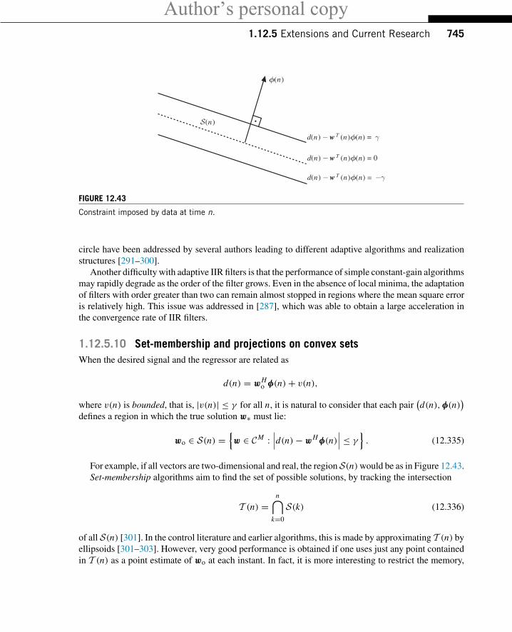
Author’s personal copy1.12.5 Extensions and Current Research 745
φ(n)
d(n) − w T (n)φ(n) = γ
d(n) − w T (n)φ(n) = −γ
d(n) − w T (n)φ(n) = 0
S(n)
FIGURE 12.43
Constraint imposed by data at time n.
circle have been addressed by several authors leading to different adaptive algorithms and realizationstructures [291–300].
Another difficulty with adaptive IIR filters is that the performance of simple constant-gain algorithmsmay rapidly degrade as the order of the filter grows. Even in the absence of local minima, the adaptationof filters with order greater than two can remain almost stopped in regions where the mean square erroris relatively high. This issue was addressed in [287], which was able to obtain a large acceleration inthe convergence rate of IIR filters.
1.12.5.10 Set-membership and projections on convex setsWhen the desired signal and the regressor are related as
d(n) = wHo φ(n)+ v(n),
where v(n) is bounded, that is, |v(n)| ≤ γ for all n, it is natural to consider that each pair(d(n),φ(n)
)defines a region in which the true solution w∗ must lie:
wo ∈ S(n) ={w ∈ CM :
∣∣∣d(n)− wH φ(n)∣∣∣ ≤ γ} . (12.335)
For example, if all vectors are two-dimensional and real, the region S(n)would be as in Figure 12.43.Set-membership algorithms aim to find the set of possible solutions, by tracking the intersection
T (n) =n⋂
k=0
S(k) (12.336)
of all S(n) [301]. In the control literature and earlier algorithms, this is made by approximating T (n) byellipsoids [301–303]. However, very good performance is obtained if one uses just any point containedin T (n) as a point estimate of wo at each instant. In fact, it is more interesting to restrict the memory,

Author’s personal copy746 CHAPTER 12 Adaptive Filters
so that the filter can track variations of wo. In this case, only the last K constraint sets S(n) are used:
TK (n) =n⋂
k=n−K+1
S(k). (12.337)
This approach has a very nice property: close to steady-state, if the weight estimates are already insideTK (n), it is not necessary to perform any update. This may reduce considerably the average complexityof the filter [304–310].
More recently, the approach has been extended to a more general setting, using projections ontoconvex sets and subgradients. This allows the extension of the results to non-differentiable cost functions,with different descriptions for the constraints (not restricted to (12.335)), also allowing the design ofkernel adaptive filters [6,311–313] (an introduction to kernel adaptive filters can be found in [314]).
1.12.5.11 Adaptive filters with constraintsIn some applications, one wishes to minimize a cost function given certain constraints: a typical case isbeamforming. In the simplest example, an array of antennas or microphones receives a signal comingfrom a certain (known) direction, and interference from other (unknown) directions. The output of thearray is a linear combination of the signals φi (n) received at each antenna, e.g.,
y(n) = w∗0φ0(n)+ w∗1φ1(n)+ · · · + w∗M−1φM−1(n).
One way of improving the signal-to-noise ratio at the output is to minimize the output power, under therestriction that the gain of the array in the direction of the desired signal is one. This is described by aconstraint of the kind
cH w = 1,
where w = [w0 . . . wM−1] is the weight vector, and c ∈ CM is a vector describing the constraint. Thegoal of the filter would then be to find the optimum wo that is the solution of
wo = arg minw
s.t. cH w=1
∣∣y(n)∣∣2 .This solution is known as minimum-variance distortionless response (MVDR), or Capon beamformer,since it was originally proposed in [315]. There is an extensive literature on this subject [312,316–325].Introductions to the topic can be found in [326–328].
1.12.5.12 Reduced-rank adaptive filtersIn applications in which large filters are necessary, such as acoustic echo cancellation and nonlinearmodels using Volterra expansions, it may be useful to reduce the order of the problem, by working ina smaller subspace of the original problem. This reduces the number of parameters to be estimated,increasing the convergence speed and reducing the excess mean-square error [329]. Several methodshave been proposed, such as [330,331], based on eigen-decompositions, the multi-stage Wiener filterof [332–334], the auxiliary vector filtering algorithm [335], and the joint iterative optimization methodof [336–339]. This last method has the advantage of having low computational cost.
Author’s personal copyReferences 747
Box 8: [Fixed-point arithmetic]
In fixed-point arithmetic, all variables are restricted to lie in a fixed interval [−a, a), and are stored as asequence of B bits b0b1 . . . bB−1. Assuming that two’s complement arithmetic is used and that a = 1 ,then b0 represents the signal of the variable and the sequence of bits represents the number
−b0 +B−1∑m=1
bm2−m .
AcknowledgmentThe authors thank Prof. Wallace A. Martins (Federal University of Rio de Janeiro) for his careful reading andcomments on the text.
Relevant Theory: Signal Processing Theory and Machine Learning
See this Volume, Chapter 3 Discrete-Time Signals and SystemsSee this Volume, Chapter 4 Random Signals and Stochastic ProcessesSee this Volume, Chapter 6 Digital Filter Structures and Their ImplementationSee this Volume, Chapter 11 Parametric EstimationSee this Volume, Chapter 25 A Tutorial on Model Selection
References[1] P.S.R. Diniz, Adaptive Filtering: Algorithms and Practical Implementation, third ed., Springer, 2008.[2] S. Haykin, Adaptive Filter Theory, fourth ed., Prentice Hall, 2001.[3] A.H. Sayed, Adaptive Filters, Wiley-IEEE Press, 2008.[4] B. Widrow, S.D. Stearns, Adaptive Signal Processing, Prentice Hall, Englewood Cliffs, 1985.[5] M.D. Miranda, M. Gerken, M.T.M. Silva, Efficient implementation of error-feedback LSL algorithm, Elec-
tron. Lett. 35 (16) (1999) 1308–1309.[6] S. Theodoridis, K. Slavakis, I. Yamada, Adaptive learning in a world of projections, IEEE Signal Process.
Mag. 28 (1) (2011) 97–123.[7] B. Widrow, M. Hoff, Adaptive switching circuits, in: IRE WESCON Conv. Rec., pt. 4, 1960, pp. 96–104.[8] B. Widrow, Thinking about thinking: the discovery of the LMS algorithm, IEEE Signal Process. Mag. 22
(1) (2005) 100–106.[9] A.V. Oppenheim, A.S. Willsky, Signals and Systems, Prentice-Hall, 1996.
[10] R.A. Horn, C.R. Johnson, Matrix Analysis, Cambridge University Press, 1987.[11] R.A. Horn, C.R. Johnson, Topics in Matrix Analysis, Cambridge University Press, Cambridge, MA, 1991.[12] A.J. Laub, Matrix Analysis for Scientists and Engineers, Society for Industrial and Applied Mathematics,
PA, December 2005.[13] C.D. Meyer, Matrix Analysis and Applied Linear Algebra, SIAM, Philadelphia, USA, 2000.[14] G.H. Golub, C.F.V. Loan, Matrix Computations, third ed., Johns Hopkins, 1996.
Author’s personal copy748 CHAPTER 12 Adaptive Filters
[15] K.J. Åström, B. Wittenmark, Adaptive Control, Addison-Wesley, 1995.[16] A. Leon-Garcia. Probability, Statistics, and Random Processes for Electrical Engineering, third ed., Prentice
Hall, January 2008.[17] T. Kailath, A.H. Sayed, B. Hassibi, Linear Estimation, Prentice Hall, NJ, 2000.[18] P. Ioannou, B. Fidan, Adaptive Control Tutorial, SIAM, Society for Industrial and Applied Mathematics,
December 2006.[19] T. Gansler, J. Benesty, New insights into the stereophonic acoustic echo cancellation problem and an adaptive
nonlinearity solution, IEEE Trans. Speech Audio Process. 10 (5) (2002) 257–267.[20] H.I.K. Rao, B. Farhang-Boroujeny, Fast LMS/Newton algorithms for stereophonic acoustic echo cancelation,
IEEE Trans. Signal Process. 57 (8) (2009) 2919–2930.[21] C.H. Hansen, S.D. Snyder, Active Control of Noise and Vibration, Taylor & Francis, 1997.[22] S.M. Kuo, D.R. Morgan, Active Noise Control Systems – Algorithms and DSP Implementations, Wiley
Series in Telecommunications and Signal Processing, Wiley-Interscience, 1996.[23] P.A. Nelson, S.J. Elliot, Active Control of Sound, Academic Press, 1992.[24] S.D. Snyder, Active Noise Control Primer, Springer-Verlag, 2000.[25] F.G. de Almeida Neto, V.H. Nascimento, M.T.M. Silva, Reduced-complexity widely linear adaptive estima-
tion, in: 7th International Symposium on Wireless Communication Systems, September 2010, pp. 399–403.[26] B. Picinbono, Wide-sense linear mean square estimation and prediction, in: International Conference on
Acoustics, Speech, and Signal Processing, 1995, ICASSP-95, vol. 3, May 1995, pp. 2032–2035.[27] B. Picinbono, P. Bondon, Second-order statistics of complex signals, IEEE Trans. Signal Process. 45 (2)
(1997) 411–420.[28] T. Adali, H. Li, R. Aloysius, On properties of the widely linear MSE filter and its LMS implementation, in:
43rd Annual Conference on Information Sciences and Systems, March 2009, pp. 876–881.[29] A. Chinatto, C. Junqueira, J.M.T. Romano, Interference mitigation using widely linear arrays, in: 17th
European Signal Processing Conference, September 2009, pp. 353–357.[30] S.C. Douglas, D.P. Mandic, Performance analysis of the conventional complex LMS and augmented complex
LMS algorithms, in: Proc. IEEE Int. Acoustics Speech and Signal Processing (ICASSP) Conf., 2010, pp.3794–3797.
[31] D.P. Mandic, S. Still, S.C. Douglas, Duality between widely linear and dual channel adaptive filtering, in:Proc. IEEE Int. Conf. Acoustics, Speech and Signal Processing, ICASSP 2009, 2009, pp. 1729–1732.
[32] P.M. Djuric, J.H. Kotecha, J. Zhang, Y. Huang, T. Ghirmai, M.F. Bugallo, J. Miguez, Particle filtering, IEEESignal Process. Mag. 20 (5) (2003) 19–38.
[33] W.R. LePage, Complex Variables and the Laplace Transform for Engineers, Dover, 1980.[34] K. Kreutz-Delgado, The complex gradient operator and the CR-Calculus, 0906.4835, June 2009.[35] W.A. Sethares, The least mean square family, in: N. Kalouptsidis, S. Theodoridis (Eds.), Adaptive System
Identification and Signal Processing Algorithms, Prentice Hall, 1993.[36] V. Solo, Averaging analysis of the LMS algorithm, in: C.T. Leondes (Ed.), Control and Dynamic Systems,
Stochastic Techniques in Digital Signal Processing Systems, Part 2 of 2, vol. 65, Academic Press, 1994, pp.379–397.
[37] B.D.O. Anderson, R.R. Bitmead, C.R.J. Johnson Jr., P.V. Kokotovic, R.L. Kosut, I.M.Y. Mareels, L. Praly,B.D. Riedle, Stability of adaptive systems: passivity and averaging analysis, MIT Press, Cambridge, MA,1986
[38] A.H. Sayed, T. Kailath, A state-space approach to adaptive RLS filtering, IEEE Signal Process. Mag. 11 (3)(1994) 18–60.
[39] H.J. Kushner, G.G. Yin, Stochastic Approximation Algorithms and Applications, Applications of Mathe-matics, Springer, 1997.
Author’s personal copyReferences 749
[40] P.A. Regalia, Numerical stability properties of a QR-based fast least squares algorithm, IEEE Trans. SignalProcess. 41 (6) (1993) 2096–2109.
[41] D.T.M. Slock, The backward consistency concept and round-off error propagation dynamics in recursiveleast-squares filtering algorithms, Opt. Eng. 31 (1992) 1153–1169.
[42] G.E. Bottomley, S.T. Alexander, A novel approach for stabilizing recursive least squares filters, IEEE Trans.Signal Process. 39 (8) (1991) 1770–1779.
[43] J.A. Apolinário Jr. (Ed.), QRD-RLS Adaptive Filtering, Springer, NY, 2009.[44] Y. Zakharov, G. White, J. Liu, Low-complexity RLS algorithms using dichotomous coordinate descent
iterations, IEEE Trans. Signal Process. 56 (7) (2008) 3150–3161.[45] V.H. Nascimento, J.C.M. Bermudez, Probability of divergence for the least-mean fourth (LMF) algorithm,
IEEE Trans. Signal Process. 54 (4) (2006) 1376–1385.[46] V.H. Nascimento, A.H. Sayed, On the learning mechanism of adaptive filters, IEEE Trans. Signal Process.
48 (6) (2000) 1609–1625.[47] S. Chen, Low complexity concurrent constant modulus algorithm and soft directed scheme for blind equal-
ization, IEE Proc. – Vis. Image Signal Process. 150 (2003) 312–320.[48] H.J. Butterweck, Iterative analysis of the steady-state weight fluctuations in LMS-type adaptive filters,
Technical Report EUT 96-E-299, Eindhoven University of Technology, Netherlands, June 1996.[49] H.J. Butterweck, A wave theory of long adaptive filters, IEEE Trans. Circ. Syst. I 48 (6) (2001) 739–747.[50] E. Eweda, O. Macchi, Convergence of an adaptive linear estimation algorithm, IEEE Trans. Autom. Control
AC-19 (2) (1984) 119–127.[51] O. Macchi, E. Eweda, Convergence analysis of self-adaptive equalizers, IEEE Trans. Inform. Theory IT-30
(2) (1984) 161–176.[52] J.E. Mazo, On the independence theory of equalizer convergence, Bell Syst. Tech. J. 58 (1979) 963–993.[53] V. Solo, X. Kong, Adaptive Signal Processing Algorithms, Prentice Hall, Englewood Cliffs, NJ, 1995.[54] S.C. Douglas, W. Pan, Exact expectation analysis of the LMS adaptive filter, IEEE Trans. Signal Process. 43
(12) (1995) 2863–2871.[55] A. Feuer, E. Weinstein, Convergence analysis of LMS filters with uncorrelated Gaussian data, IEEE Trans.
Acoust. Speech Signal Process. ASSP-33 (1) (1985) 222–229.[56] S. Florian, A. Feuer, Performance analysis of the LMS algorithm with a tapped delay
line (two-dimensional case), IEEE Trans. Acoust. Speech Signal Process. ASSP-34 (6) (1986)1542–1549.
[57] A.H. Sayed, V.H. Nascimento, Energy conservation and the learning ability of LMS adaptive filters, in: S.Haykin, B. Widrow (Eds.), Least-Mean-Square Adaptive Filters, Wiley, 2003.
[58] O. Dabeer, E. Masry, Convergence analysis of the constant modulus algorithm, IEEE Trans. Inform. Theory49 (6) (2003) 1447–1464.
[59] P.I. Hübscher, J.C.M. Bermudez, V.H. Nascimento, A mean-square stability analysis of the least mean fourth(LMF) adaptive algorithm, IEEE Trans. Signal Process. 55 (8) (2007) 4018–4028.
[60] V.H. Nascimento, M.T.M. Silva, Stochastic stability analysis for the constant-modulus algorithm, IEEETrans. Signal Process. 56 (10) (2008) 4984–4989.
[61] T.Y. Al-Naffouri, M. Moinuddin, Exact performance analysis of the ε-NLMS algorithm for colored circularGaussian inputs, IEEE Trans. Signal Process. 58 (10) (2010) 5080–5090.
[62] T.Y. Al-Naffouri, M. Moinuddin, M.S. Sohail, Mean weight behavior of the NLMS algorithm for correlatedGaussian inputs, IEEE Signal Process. Lett. 18 (1) (2011) 7–10.
[63] N.J. Bershad, Analysis of the normalized LMS algorithm with Gaussian inputs, IEEE Trans. Acoust. SpeechSignal Process. ASSP-34 (1986) 793–806.
[64] N.J. Bershad, Behavior of the ε-normalized LMS algorithm with Gaussian inputs, IEEE Trans. Acoust.Speech Signal Process. ASSP-35, May 1987, pp. 636–644.
Author’s personal copy750 CHAPTER 12 Adaptive Filters
[65] M.H. Costa, J.C.M. Bermudez, An improved model for the normalized LMS algorithm with Gaussian inputsand large number of coefficients, in: Proc. ICASSP 2002, vol. 2, pp. 1385–1388.
[66] V.H. Nascimento, A simple model for the effect of normalization on the convergence rate of adaptive filters,in: Proc. of the 2004 IEEE International Conference on Acoustics, Speech and, Signal Processing, 2004, pp.II-453–II-456.
[67] D.T.M. Slock, On the convergence behavior of the LMS and the normalized LMS algorithms, IEEE Trans.Signal Process. 41 (9) (1993) 2811–2825.
[68] M. Tarrab, A. Feuer, Convergence and performance analysis of the normalized LMS algorithm with uncor-related Gaussian data, IEEE Trans. Inform. Theory 34 (4) (1988) 680–691.
[69] A. Carini, E. Mumolo, G.L. Sicuranza, V-vector algebra and its application to Volterra-adaptive filtering,IEEE Trans. Circ. Syst. II 46 (5) (1999) 585–598.
[70] F. Kuech, W. Kellermann, Orthogonalized power filters for nonlinear acoustic echo cancellation, SignalProcess. 86 (6) (2006) 1168–1181.
[71] V.J. Mathews, G.L. Sicuranza, Polynomial Signal Processing, Wiley-Interscience, New York, 2000.[72] A. Stenger, W. Kellermann, Adaptation of a memoryless preprocessor for nonlinear acoustic echo cancelling,
Signal Process. 80 (9) (2000) 1747–1760.[73] G.L. Sicuranza, A. Carini, A. Fermo, Nonlinear adaptive filters for acoustic echo cancellation in mobile
terminals, in: K.E. Barner, G.R. Arce (Eds.), Nonlinear Signal and Image Processing: Theory, Methods,and Applications, The Electrical Engineering and Applied Signal Processing Series, CRC Press, 2003, pp.223–255 (Chapter 7).
[74] E. Eleftheriou, D. Falconer, Tracking properties and steady-state performance of RLS adaptive filter algo-rithms, IEEE Trans. Acoust. Speech Signal Process. 34 (5) (1986) 1097–1110.
[75] G.V. Moustakides, Study of the transient phase of the forgetting factor RLS, IEEE Trans. Signal Process. 45(10) (1997) 2468–2476.
[76] A.H. Sayed, M. Rupp, Error-energy bounds for adaptive gradient algorithms, IEEE Trans. Signal Process.44 (8) (1996) 1982–1989.
[77] N. Yousef, A.H. Sayed, A unified approach to the steady-state and tracking analysis of adaptive filters, IEEETrans. Signal Process. 49 (2) (2001) 314–324.
[78] M. Rupp, A.H. Sayed, A time-domain feedback analysis of filtered-error adaptive gradient algorithms, IEEETrans. Signal Process. 44 (1996) 1428–1439.
[79] C. Samsom, V.U. Reddy, Fixed point error analysis of the normalized ladder algorithm, IEEE Trans. Acoust.Speech, Signal Process. 31 (5) (1983) 1177–1191.
[80] J.Y. Mai, A.H. Sayed, A feedback approach to the steady-state performance of fractionally spaced blindadaptive equalizers, IEEE Trans. Signal Process. 48 (1) (2000) 80–91.
[81] E. Eweda, Comparison of RLS, LMS, and sign algorithms for tracking randomly time-varying channels,IEEE Trans. Signal Process. 42 (11) (1994) 2937–2944.
[82] J.H. Wilkinson, Rounding Errors in Algebraic Processes, Her Majesty’s Stationery Office, 1963.[83] J.H. Wilkinson, The Algebraic Eigenvalue Problem, Oxford University Press, London, UK, 1965.[84] S.T. Alexander, Transient weight misadjustment properties for the finite precision LMS algorithm, IEEE
Trans. Acoust. Speech Signal Process. ASSP-35 (9) (1987) 1250–1258.[85] S. Ardalan, Floating-point error analysis of recursive least-squares and least-mean-squares adaptive filters,
IEEE Trans. Circ. Syst. 33 (12) (1986) 1192–1208.[86] C. Caraiscos, B. Liu, A roundoff error analysis of the LMS adaptive algorithm, IEEE Trans. Acoust. Speech
Signal Process. ASSP-32 (1) (1984) 34–41.[87] R.D. Gitlin, J.E. Mazo, M.G. Taylor, On the design of gradient algorithms for digitally implemented adaptive
filters, IEEE Trans. Circ. Theory, CT-20 (2) (1973) 125–136.
Author’s personal copyReferences 751
[88] J.C.M. Bermudez, N.J. Bershad, A nonlinear analytical model for the quantized LMS algorithm the arbitrarystep size case, IEEE Trans. Signal Process. 44 (5) (1996) 1175–1183.
[89] J.C.M. Bermudez, N.J. Bershad, Transient and tracking performance analysis of the quantized LMS algorithmfor time-varying system identification, IEEE Trans. Signal Process. 44 (8) (1996) 1990–1997.
[90] N.J. Bershad, J.C. Bermudez, New insights on the transient and steady-state behavior of the quantized LMSalgorithm, IEEE Trans. Signal Process. 44 (10) (1996) 2623–2625.
[91] N.J. Bershad, J.C.M. Bermudez, A nonlinear analytical model for the quantized LMS algorithm-the power-of-two step size case, IEEE Trans. Signal Process. 44 (11) (1996) 2895–2900.
[92] J.M. Cioffi, J.J. Werner, The tap-drifting problem in digitally implemented data-driven echo cancellers, BellSyst. Tech. J. 64 (1) (1985) 115–138.
[93] R.D. Gitlin, H.C. Meadors Jr., S.B. Weinstein, The tap-leakage algorithm: an algorithm for the stable operationof a digitally implemented, fractionally spaced adaptive equalizer, Bell Syst. Tech. J. 61 (8) (1982) 1817–1839.
[94] V.H. Nascimento, A.H. Sayed, Unbiased and stable leakage-based adaptive filters, IEEE Trans. Signal Pro-cess. 47 (12) (1999) 3261–3276.
[95] E. Eweda, Almost sure convergence of a decreasing gain sign algorithm for adaptive filtering, IEEE Trans.Acoust. Speech Signal Process. 36 (10) (1988) 1669–1671.
[96] E. Eweda, A tight upper bound of the average absolute error in a constant step-size sign algorithm, IEEETrans. Acoust. Speech Signal Process. 37 (11) (1989) 1774–1776.
[97] E. Eweda, Convergence analysis of the sign algorithm without the independence and Gaussian assumptions,IEEE Trans. Signal Process. 48 (9) (2000) 2535–2544.
[98] A. Gersho, Adaptive filtering with binary reinforcement, IEEE Trans. Inform. Theory 30 (2) (1984) 191–199.[99] P. Xue, B. Liu, Adaptive equalizer using finite-bit power-of-two quantizer, IEEE Trans. Acoust. Speech
Signal Process. 34 (6) (1986) 1603–1611.[100] S. Ljung, L. Ljung, Error propagation properties of recursive least-squares adaptation algorithms, Automatica
21 (2) (1985) 157–167.[101] J. Cioffi, The fast adaptive ROTOR’s RLS algorithm, IEEE Trans. Acoust. Speech Signal Process. 38 (4)
(1990) 631–653.[102] S. Alexander, A. Ghimikar, A method for recursive least squares filtering based upon an inverse QR decom-
position, IEEE Trans. Signal Process. 41 (1) (1993) 20.[103] S.T. Alexander, A.L. Ghimikar, A method for recursive least squares filtering based upon an inverse QR
decomposition, IEEE Trans. Signal Process. 41 (1) (1993).[104] J.A. Apolinário Jr., P. Diniz, A new fast QR algorithm based on a priori errors, IEEE Signal Process. Lett. 4
(11) (1997) 307–309.[105] M.D. Miranda, L. Aguayo, M. Gerken. Performance of the a priori and a posteriori QR-LSL algorithms in
a limited precision environment, in: Proc. IEEE Int Acoustics, Speech, and Signal Processing ICASSP-97Conf., vol. 3, 1997, pp. 2337–2340.
[106] M.D. Miranda, M. Gerken, A hybrid QR-lattice least squares algorithm using a priori errors, in: Proc. 38thMidwest Symp. Circuits and Systems, Proceedings, vol. 2, 1995, pp. 983–986.
[107] M.D. Miranda, M. Gerken, A hybrid least squares QR-lattice algorithm using a priori errors, IEEE Trans.Signal Process. 45 (12) (1997) 2900–2911.
[108] I.K. Proudler, J.G. McWhirter, T.J. Shepherd, Computationally efficient QR decomposition approach to leastsquares adaptive filtering, IEE Proc. F Radar Signal Process. 138 (4) (1991) 341–353.
[109] P.A. Regalia, M.G. Bellanger, On the duality between fast QR methods and lattice methods in least-squaresadaptive filtering, IEEE Trans. Signal Process. 39 (1991) 879–891.
[110] A. Rontogiannis, S. Theodoridis, On inverse factorization adaptive LS algorithms, Signal Process. 52 (1997)35–47.
Author’s personal copy752 CHAPTER 12 Adaptive Filters
[111] A.A. Rontogiannis, S. Theodoridis, New fast inverse QR least squares adaptive algorithms, in: Proc. Int.Acoustics, Speech, and Signal Processing, vol. 2, 1995, pp. 1412–1415.
[112] A.A. Rontogiannis, S. Theodoridis, New multichannel fast QRD-LS adaptive algorithms, in: Proc. 13th Int.Conf. Digital Signal Processing, vol. 1, 1997, pp. 45–48.
[113] A.A. Rontogiannis, S. Theodoridis, Multichannel fast QRD-LS adaptive filtering: new technique and algo-rithms, IEEE Trans. Signal Process. 46 (11) (1998) 2862–2876.
[114] A.A. Rontogiannis, S. Theodoridis, New fast QR decomposition least squares adaptive algorithms, IEEETrans. Signal Process. 46 (8) (1998) 2113–2121.
[115] M. Shoaib, S. Werner, J.A. Apolinário, Multichannel fast QR-decomposition algorithms: weight extractionmethod and its applications, IEEE Trans. Signal Process. 58 (1) (2010) 175–188.
[116] M. Shoaib, S. Werner, J.A. Apolinário, T.I. Laakso, Solution to the weight extraction problem in fast QR-decomposition rls algorithms, in: Proc. IEEE Int. Acoustics, Speech and Signal Processing Conf., ICASSP2006, vol. 3, 2006.
[117] B. Friedlander, Lattice filters for adaptive processing, IEEE Trans. Signal Process. 70 (8) (1982) 829–867.[118] D. Lee, M. Morf, B. Friedlander, Recursive least squares ladder estimation algorithms, IEEE Trans. Circ.
Syst. 28 (6) (1981) 467–481.[119] H. Lev-Ari, T. Kailath, J. Cioffi, Least-squares adaptive lattice and transversal filters: a unified geometric
theory, IEEE Trans. Inform. Theory 30 (2) (1984) 222–236.[120] F. Ling, D. Manolakis, J. Proakis, Numerically robust least-squares lattice-ladder algorithms with direct
updating of the reflection coefficients, IEEE Trans. Acoust. Speech Signal Process. 34 (4) (1986) 837–845.[121] V.J. Mathews, Z. Xie, Fixed-point error analysis of stochastic gradient adaptive lattice filters, IEEE Trans.
Acoust. Speech Signal Process. 38 (1) (1990) 70–80.[122] R.C. North, J.R. Zeidler, W.H. Ku, T.R. Albert, A floating-point arithmetic error analysis of direct and
indirect coefficient updating techniques for adaptive lattice filters, IEEE Trans. Signal Process. 41 (5) (1993)1809–1823.
[123] M.J. Reed, B. Liu, Analysis of simplified gradient adaptive lattice algorithms using power-of-two quantiza-tion, in: Proc. IEEE Int. Circuits and Systems Symp., 1990, pp. 792–795.
[124] C. Samson, V. Reddy, Fixed point error analysis of the normalized ladder algorithm, IEEE Trans. Acoust.Speech Signal Process. 31 (5) (1983) 1177–1191.
[125] R. Merched, Extended RLS lattice adaptive filters, IEEE Trans. Signal Process. 51 (9) (2003) 2294–2309.[126] R. Merched, A.H. Sayed, Order-recursive RLS laguerre adaptive filtering, IEEE Trans. Signal Process. 48
(11) (2000) 3000–3010.[127] R. Merched, A.H. Sayed, RLS-Laguerre lattice adaptive filtering: error-feedback, normalized, and array-
based algorithms, IEEE Trans. Signal Process. 49 (11) (2001) 2565–2576.[128] J.-L. Botto, G.V. Moustakides, Stabilizing the fast Kalman algorithms, IEEE Trans. Acoust. Speech Signal
Process. 37 (9) (1989) 1342–1348.[129] J. Cioffi, T. Kailath, Fast, recursive-least-squares transversal filters for adaptive filtering, IEEE Trans. Acoust.
Speech Signal Process. 32 (2) (1984) 304–337.[130] J. Cioffi, T. Kailath, Windowed fast transversal filters adaptive algorithms with normalization, IEEE Trans.
Acoust. Speech Signal Process. 33 (3) (1985) 607–625.[131] D. Falconer, L. Ljung, Application of fast Kalman estimation to adaptive equalization, IEEE Trans. Commun.
26 (10) (1978) 1439–1446.[132] G.V. Moustakides, S. Theodorides, Fast Newton transversal filters a new class of adaptive estimation algo-
rithms, IEEE Trans. Signal Process. 39 (10) (1991) 2184–2193.[133] D.T.M. Slock, T. Kailath, Fast transversal filters with data sequence weighting, IEEE Trans. Acoust., Speech
Signal Process. 37 (3) (1989) 346–359.
Author’s personal copyReferences 753
[134] D.T.M. Slock, T. Kailath, Numerically stable fast transversal filters for recursive least squares adaptivefiltering, IEEE Trans. Signal Process. 39 (1) (1991) 92–114.
[135] Y. Zakharov, T. Tozer, Multiplication-free iterative algorithm for LS problem, Electron. Lett. 40 (9) (2004)567–569.
[136] W.A. Sethares, D.A. Lawrence, C.R. Johnson Jr., R.R. Bitmead, Parameter drift in LMS adaptive filters,IEEE Trans. Acoust. Speech Signal Process. ASSP-34 (1986) 868–878.
[137] K. Mayyas, T. Aboulnasr, The leaky LMS algorithm: MSE analysis for Gaussian data, IEEE Trans. SignalProcess. 45 (4) (1997) 927–934.
[138] C.S. Ludovico, J.C.M. Bermudez, A recursive least squares algorithm robust to low-power excitation,in: IEEE International Conference on Acoustics, Speech, and Signal Processing, 2004, Proceedings(ICASSP’04), 2004.
[139] J. Liu, Y. Zakharov, Low complexity dynamically regularised RLS algorithm, Electron. Lett. 44 (14) (2008)885–886.
[140] M.C. Tsakiris, C.G. Lopes, V.H. Nascimento, An array recursive least-squares algorithm with generic non-fading regularization matrix, IEEE Signal Process. Lett. 17 (12) (2010) 1001–1004.
[141] N. Jablon, Adaptive beamforming with the generalized sidelobe canceller in the presence of array imperfec-tions, IEEE Trans. Antennas Propag. 34 (8) (1986) 996–1012.
[142] J.C.M. Bermudez, M.H. Costa, Optimum leakage factor for the MOV-LMS algorithm in nonlinear modelingand control systems, in: Proc. IEEE Int Acoustics, Speech, and Signal Processing (ICASSP) Conf., vol. 2,2002.
[143] E.J. Candès, M.B. Wakin, People hearing without listening: an introduction to compressive sampling, IEEESignal Process. Mag. 25 (2) (2008) 21–30.
[144] D. Angelosante, J.A. Bazerque, G.B. Giannakis, Online adaptive estimation of sparse signals: where RLSmeets the �1-norm, IEEE Trans. Signal Process. 58 (7) (2010) 3436–3447.
[145] D. Angelosante, G.B. Giannakis, RLS-weighted Lasso for adaptive estimation of sparse signals, in: Proc.IEEE Int. Conf. Acoustics, Speech and Signal Processing, ICASSP 2009, 2009, pp. 3245–3248.
[146] Y. Chen, Y. Gu, A.O. Hero, Sparse LMS for system identification, in: Proc. ICASSP 2009, April 2009, pp.3125–3128.
[147] Y. Kopsinis, K. Slavakis, S. Theodoridis, Online sparse system identification and signal reconstruction usingprojections onto weighted �1 balls, IEEE Trans. Signal Process. 59 (3) (2011) 936–952.
[148] G. Mileounis, B. Babadi, N. Kalouptsidis, V. Tarokh, An adaptive greedy algorithm with application tononlinear communications, IEEE Trans. Signal Process. 58 (6) (2010) 2998–3007.
[149] R. Harris, D. Chabries, F. Bishop, A variable step (VS) adaptive filter algorithm, IEEE Trans. Acoust. SpeechSignal Process. 34 (2) (1986) 309–316.
[150] B. Farhang-Boroujeny, Adaptive Filters – Theory and Applications, John Wiley & Sons, West Sussex, 1998.[151] J. Nagumo, A. Noda, A learning method for system identification, IEEE Trans. Autom. Control 12 (3) (1967)
282–287.[152] A.E. Albert, L.S. Gardner Jr., Stochastic Approximation and Nonlinear Regression, MIT Press, 1967.[153] T. Aboulnasr, K. Mayyas, A robust variable step-size LMS-type algorithm, IEEE Trans. Signal Process. 45
(3) (1997) 631–639.[154] W.-P. Ang, B. Farhang-Boroujeny, A new class of gradient adaptive step-size LMS algorithms, IEEE Trans.
Signal Process. 49 (4) (2001) 805–810.[155] J. Benesty, H. Rey, L. Vega, S. Tressens, A nonparametric VSS NLMS algorithm, IEEE Signal Process. Lett.
13 (10) (2006) 581–584.[156] N. Bershad, On the optimum gain parameter in LMS adaptation, IEEE Trans. Acoust. Speech Signal Process.
35 (7) (1987) 1065–1068.
Author’s personal copy754 CHAPTER 12 Adaptive Filters
[157] R.C. Bilcu, P. Kuosmanen, K. Egiazarian, A transform domain LMS adaptive filter with variable step-size,IEEE Signal Process. Lett. 9 (2) (2002) 51–53.
[158] J.B. Evans, P. Xue, B. Liu, Analysis and implementation of variable step size adaptive algorithms, IEEETrans. Signal Process. 41 (8) (1993) 2517–2535.
[159] B. Farhang-Boroujeny, Variable-step-size LMS algorithm: new developments and experiments, IEE Proc.Vis. Image Signal Process. 141 (5) (1994) 311–317.
[160] A. Gupta, S. Joshi, Variable step-size LMS algorithm for fractal signals, IEEE Trans. Signal Process. 56 (4)(2008) 1411–1420.
[161] R.H. Kwong, E.W. Johnston, A variable step size LMS algorithm, IEEE Trans. Signal Process. 40 (7) (1992)1633–1642.
[162] V.J. Mathews, Z. Xie, A stochastic gradient adaptive filter with gradient adaptive step size, IEEE Trans.Signal Process. 41 (6) (1993) 2075–2087.
[163] C. Paleologu, J. Benesty, S. Ciochina, A robust variable forgetting factor recursive least-squares algorithmfor system identification, IEEE Signal Process. Lett. 15 (2008) 597–600.
[164] C. Paleologu, S. Ciochina, J. Benesty, Variable step-size NLMS algorithm for under-modeling acoustic echocancellation, IEEE Signal Process. Lett. 15 (2008) 5–8.
[165] D.I. Pazaitis, A.G. Constantinides, A novel kurtosis driven variable step-size adaptive algorithm, IEEE Trans.Signal Process. 47 (3) (1999) 864–872.
[166] H.-C. Shin, A.H. Sayed, W.-J. Song, Variable step-size NLMS and affine projection algorithms, IEEE SignalProcess. Lett. 11 (2) (2004) 132–135.
[167] L. Vega, H. Rey, J. Benesty, S. Tressens, A new robust variable step-size NLMS algorithm, IEEE Trans.Signal Process. 56 (5) (2008) 1878–1893.
[168] J. Benesty, S.L. Gay, An improved PNLMS algorithm, in: International Conference on Acoustics, Speechand Signal Processing, vol. 2, IEEE, 2002, pp. 1881–1884.
[169] F. das Chagas de Souza, O.J. Tobias, R. Seara, D.R. Morgan, A PNLMS algorithm with individual activationfactors, IEEE Trans. Signal Process. 58 (4) (2010) 2036–2047.
[170] F. das Chagas de Souza, O.J. Tobias, R. Seara, D.R. Morgan, Stochastic model for the mean weight evolutionof the IAF-PNLMS algorithm, IEEE Trans. Signal Process. 58 (11) (2010) 5895–5901.
[171] D.L. Duttweiler, Proportionate normalized least-mean-squares adaptation in echo cancellers, IEEE Trans.Speech Audio Process. 8 (5) (2000) 508–518.
[172] T. Gansler, S.L. Gay, M.M. Sondhi, J. Benesty, Double-talk robust fast converging algorithms for networkecho cancellation, IEEE Trans. Speech Audio Process. 8 (6) (2000) 656–663.
[173] E. Walach, B. Widrow, The least mean fourth (LMF) adaptive algorithm and its family, IEEE Trans. Inform.Theory IT-30 (2) (1984) 275–283.
[174] R. Sharma, W.A. Sethares, J.A. Bucklew, Asymptotic analysis of stochastic gradient-based adaptive filteringalgorithms with general cost functions, IEEE Trans. Signal Process. 44 (9) (1996) 2186–2194.
[175] T.Y. Al-Naffouri, A.H. Sayed, Transient analysis of adaptive filters with error nonlinearities, IEEE Trans.Signal Process. 51 (3) (2003) 653–663.
[176] J.A. Chambers, O. Tanrikulu, A.G. Constantinides, Least mean mixed-norm adaptive filtering, Electron. Lett.30 (19) (1994).
[177] O. Tanrikulu, J.A. Chambers, Convergence and steady-state properties of the least-mean mixed-norm(LMMN) adaptive algorithm, IEEE Trans. Signal Process. 143 (3) (1996) 137–142.
[178] A.H. Sayed, Fundamentals of Adaptive Filtering, Wiley-Interscience, 2003.[179] B. Hassibi, A.H. Sayed, T. Kailath, LMS is H∞-optimal, in: Proc. Conference on Decision and Control,
San Antonio, TX, vol. 1, December 1993, pp. 74–79.[180] G. Aydin, O. Arikan, A.E. Cetin, Robust adaptive filtering algorithms for α-stable random processes, IEEE
Trans. Circ. Syst. II 46 (2) (1999) 198–202.
Author’s personal copyReferences 755
[181] S.R. Kim, A. Efron, Adaptive robust impulse noise filtering, IEEE Trans. Signal Process. 43 (8) (1995)1855–1866.
[182] E. Masry, Alpha-stable signals and adaptive filtering, IEEE Trans. Signal Process. 48 (11) (2000) 3011–3016.[183] M. Shao, C.L. Nikias, Signal processing with fractional lower order moments: stable processes and their
applications, Proc. IEEE 81 (7) (1993) 986–1010.[184] D. Hirsch, W. Wolf, A simple adaptive equalizer for efficient data transmission, IEEE Trans. Commun.
Technol. 18 (1) (1970) 5–12.[185] A. Flaig, G.R. Arce, K.E. Barner, Affine order-statistic filters: medianization of linear FIR filters, IEEE
Trans. Signal Process. 46 (8) (1998) 2101–2112.[186] D.N. Godard, Self-recovering equalization and carrier tracking in two-dimensional data communication
systems, IEEE Trans. Commun. 28 (11) (1980) 1867–1875.[187] J.R. Treichler, B. Agee, A new approach to multipath correction of constant modulus signals, IEEE Trans.
Acoust. Speech Signal Process. ASSP-28 (1983) 334–358.[188] C.B. Papadias, D.T.M. Slock, Normalized sliding window constant modulus and decision-direct algorithms:
a link between blind equalization and classical adaptive filtering, IEEE Trans. Signal Process. 45 (1997)231–235.
[189] Z. Ding, Y. Li, Blind Equalization and Identification, Marcel Dekke, 2001.[190] M.T.M. Silva, V.H. Nascimento, Improving the tracking capability of adaptive filters via convex combination,
IEEE Trans. Signal Process. 56 (7) (2008) 3137–3149.[191] C.R. Johnson Jr., P. Schniter, T.J. Endres, J.D. Behm, D.R. Brown, R.A. Casas, Blind equalization using the
constant modulus criterion: a review, Proc. IEEE 86 (10) (1998) 1927–1950.[192] R. Candido, M.T.M. Silva, M.D. Miranda, V.H. Nascimento, A statistical analysis of the dual-mode CMA,
in: Proc. IEEE Int. Circuits and Systems (ISCAS) Symp., 2010, pp. 2510–2513.[193] R. Candido, M.T.M. Silva, V.H. Nascimento, Transient and steady-state analysis of the affine combination
of two adaptive filters, IEEE Trans. Signal Process. 58 (8) (2010) 4064–4078.[194] I. Fijalkow, C.E. Manlove, C.R. Johnson Jr., Adaptive fractionally spaced blind CMA equalization: excess
MSE, IEEE Trans. Signal Process. 46 (1) (1998) 227–231.[195] M.T.M. Silva, M.D. Miranda, Tracking issues of some blind equalization algorithms, IEEE Signal Process.
Lett. 11 (9) (2004) 760–763.[196] M.T.M. Silva, V.H. Nascimento, Tracking analysis of the constant modulus algorithm, in: Proc., ICASSP
2008, Las Vegas, NV, USA, pp. 3561–3564.[197] M.D. Miranda, M.T.M. Silva, V.H. Nascimento, Avoiding divergence in the constant modulus algorithm, in:
Proc., ICASSP 2008, Las Vegas, NV, USA, 2008, pp. 3565–3568.[198] M.D. Miranda, M.T.M. Silva, V.H. Nascimento, Avoiding divergence in the Shalvi-Weinstein algorithm,
IEEE Trans. Signal Process. 56 (11) (2008) 5403–5413.[199] P.A. Regalia, M. Mboup, Undermodeled equalization: a characterization of stationary points for a family of
blind criteria, IEEE Trans. Signal Process. 47 (1999) 760–770.[200] R. Suyama, R.R.F. Attux, J.M.T. Romano, M. Bellanger, On the relationship between least squares and
constant modulus criteria for adaptive filtering, in: The 37th Asilomar Conference on Signals, Systems andComputers, vol. 2, 2003, pp. 1293–1297.
[201] J. Yang, J.-J. Werner, G.A. Dumont, The multimodulus blind equalization and its generalized algorithms,IEEE J. Sel. Areas Commun. 20 (2002) 997–1015.
[202] J.-T. Yuan, T.-C. Lin, Equalization and carrier phase recovery of CMA and MMA in blind adaptive receivers,IEEE Trans. Signal Process. 58 (6) (2010) 3206–3217.
[203] J.-T. Yuan, K.-D. Tsai, Analysis of the multimodulus blind equalization algorithm in QAM communicationsystems, IEEE Trans. Commun. 53 (2005) 1427–1431.
Author’s personal copy756 CHAPTER 12 Adaptive Filters
[204] S. Abrar, A. Nandi, Blind equalization of square-QAM signals: a multimodulus approach, IEEE Trans.Commun. 58 (6) (2010) 1674–1685.
[205] K. Banovic, E. Abdel-Raheem, M.A.S. Khalid, A novel radius-adjusted approach for blind adaptive equal-ization, IEEE Signal Process. Lett. 13 (2006) 37–40.
[206] J. Mendes Filho, M.T.M. Silva, M.D. Miranda, A family of algorithms for blind equalization of QAMsignals, in: Proc. IEEE Int. Conf. Acoustics, Speech, and Signal Process, Prague, Czech Republic, 2011, pp.3388–3391.
[207] J. Mendes Filho, M.T.M. Silva, M.D. Miranda, V.H. Nascimento, A region-based algorithm for blind equal-ization of QAM signals, in: Proc. of the IEEE/SP 15th Workshop on Statistical Signal Processing, Cardiff,UK, 2009, pp. 685–688.
[208] F. Beaufays, Transform-domain adaptive filters: an analytical approach, IEEE Trans. Signal Process. 43 (2)(1995) 422–431.
[209] G. Clark, S. Mitra, S. Parker, Block implementation of adaptive digital filters, IEEE Trans. Acoust. SpeechSignal Process. 29 (3) (1981) 744–752.
[210] B. Farhang-Boroujeny, Analysis and efficient implementation of partitioned block LMS adaptive filters,IEEE Trans. Signal Process. 44 (11) (1996) 2865–2868.
[211] E. Ferrara, Fast implementations of LMS adaptive filters, IEEE Trans. Acoust. Speech Signal Process. 28(4) (1980) 474–475.
[212] R. Merched, A.H. Sayed, An embedding approach to frequency-domain and subband adaptive filtering, IEEETrans. Signal Process. 48 (9) (2000) 2607–2619.
[213] S. Narayan, A. Peterson, M. Narasimha, Transform domain LMS algorithm, IEEE Trans. Acoust. SpeechSignal Process. 31 (3) (1983) 609–615.
[214] S.S. Narayan, A.M. Peterson, Frequency domain least-mean-square algorithm, Proc. IEEE 69 (1) (1981)124–126.
[215] J.J. Shynk, Frequency-domain and multirate adaptive filtering, IEEE Signal Process. Mag. 9 (1) (1992)14–37.
[216] J.-S. Soo, K.K. Pang, Multidelay block frequency domain adaptive filter, IEEE Trans. Acoust. Speech SignalProcess. 38 (2) (1990) 373–376.
[217] P.P. Vaidyanathan, Multirate Systems and Filter Banks, Prentice Hall, Englewood Cliffs, NJ, 1993.[218] I. Furukawa, A design of canceller of broadband acoustic echo, in: Proc. Int. Teleconference Symposium,
Tokyo, Japan, 1984, pp. 1–8.[219] A. Gilloire, M. Vetterli, Adaptive filtering in subbands with critical sampling: analysis, experiments, and
application to acoustic echo cancellation, IEEE Trans. Signal Process. 40 (8) (1992) 1862–1875.[220] W. Kellermann, Kompensation akustischer Echos in Frequenzteilbändern, Frequenz 39 (1985) 209–215.[221] M.R. Petraglia, R.G. Alves, P.S.R. Diniz, New structures for adaptive filtering in subbands with critical
sampling, IEEE Trans. Signal Process. 48 (12) (2000) 3316–3327.[222] M.R. Petraglia, P.B. Batalheiro, Nonuniform subband adaptive filtering with critical sampling, IEEE Trans.
Signal Process. 56 (2) (2008) 565–575.[223] M.R. Petraglia, S.K. Mitra, Adaptive fir filter structure based on the generalized subband decomposition of
fir filters, IEEE Trans. Circ. Syst. II 40 (6) (1993) 354–362.[224] S. Weiss, R.W. Stewart, R. Rabenstein, Steady-state performance limitations of subband adaptive filters,
IEEE Trans. Signal Process. 49 (9) (2001) 1982–1991.[225] N. Hirayama, H. Sakai, S. Miyagi, Delayless subband adaptive filtering using the Hadamard transform, IEEE
Trans. Signal Process. 47 (6) (1999) 1731–1734.[226] R. Merched, M. Petraglia, P.S.R. Diniz, A delayless alias-free subband adaptive filter structure, IEEE Trans.
Signal Process. 47 (6) (1999) 1580–1591.
Author’s personal copyReferences 757
[227] D.R. Morgan, J.C. Thi, A delayless subband adaptive filter architecture, IEEE Trans. Signal Process. 43 (8)(1995) 1819–1830.
[228] K. Nishikawa, H. Kiya, Conditions for convergence of a delayless subband adaptive filter and its efficientimplementation, IEEE Trans. Signal Process. 46 (4) (1998) 1158–1167.
[229] J. Apolinário Jr., M.L.R. Campos, P.S.R. Diniz, Convergence analysis of the binormalized data-reusing LMSalgorithm, IEEE Trans. Signal Process. 48 (11) (2000) 3235–3242.
[230] S.G. Kratzer, D.R. Morgan, The partial-rank algorithm for adaptive beamforming, in: Proc. SPIE, vol. 564,1985, pp. 9–14.
[231] D.R. Morgan, S.G. Kratzer, On a class of computationally efficient, rapidly converging, generalized NLMSalgorithms, IEEE Signal Process. Lett. 3 (8) (1996) 245–247.
[232] K. Ozeki, T. Umeda, An adaptive filtering algorithm using an orthogonal projection to an affine subspaceand its properties, Electron. Commun. Jpn. 67-A (1984) 19–27.
[233] S. Roy, J.J. Shynk, Analysis of the data-reusing LMS algorithm, in: Proc. 32nd Midwest Symp. Circuits andSystems, 1989, pp. 1127–1130.
[234] M. Rupp, A family of adaptive filter algorithms with decorrelating properties, IEEE Trans. Signal Process.46 (3) (1998) 771–775.
[235] S.L. Gay, S. Tavathia, The fast affine projection algorithm, in: Proc. Int. Acoustics, Speech, and SignalProcessing ICASSP-95 Conf., vol. 5, 1995, pp. 3023–3026.
[236] G. Rombouts, M. Moonen, A fast exact frequency domain implementation of the exponentially windowedaffine projection algorithm, in: Proc. and Control Symp Adaptive Systems for Signal Processing, Commu-nications 2000, AS-SPCC, The IEEE 2000, 2000, pp. 342–346.
[237] M. Tanaka, S. Makino, J. Kojima, A block exact fast affine projection algorithm, IEEE Trans. Speech AudioProcess. 7 (1) (1999) 79–86.
[238] S.J.M. de Almeida, J.C.M. Bermudez, N.J. Bershad, A stochastic model for a pseudo affine projectionalgorithm, IEEE Trans. Signal Process. 57 (1) (2009) 107–118.
[239] S.J.M. de Almeida, J.C.M. Bermudez, N.J. Bershad, M.H. Costa, A statistical analysis of the affine projectionalgorithm for unity step size and autoregressive inputs, IEEE Trans. Circ. Syst. I 52 (7) (2005) 1394–1405.
[240] S.G. Sankaran, A.A.L. Beex, Convergence behavior of affine projection algorithms, IEEE Trans. SignalProcess. 48 (4) (2000) 1086–1096.
[241] H.-C. Shin, A.H. Sayed, Mean-square performance of a family of affine projection algorithms, IEEE Trans.Signal Process. 52 (1) (2004) 90–102.
[242] C. Paleologu, J. Benesty, S. Ciochina, Regularization of the affine projection algorithm, IEEE Trans. Circ.Syst. II 58 (6) (2011) 366–370.
[243] H. Rey, L.R. Vega, S. Tressens, J. Benesty, Variable explicit regularization in affine projection algorithm:robustness issues and optimal choice, IEEE Trans. Signal Process. 55 (5) (2007) 2096–2109.
[244] J. Benesty, P. Duhamel, Y. Grenier, A multichannel affine projection algorithm with applications to multi-channel acoustic echo cancellation, IEEE Signal Process. Lett. 3 (2) (1996) 35–37.
[245] C. Paleologu, J. Benesty, S. Ciochina, A variable step-size affine projection algorithm designed for acousticecho cancellation, IEEE Trans. Audio Speech Lang. Process. 16 (8) (2008) 1466–1478.
[246] D. Manolakis, F. Ling, J. Proakis, Efficient time-recursive least-squares algorithms for finite-memory adaptivefiltering, IEEE Trans. Circ. Syst. 34 (4) (1987) 400–408.
[247] K. Maouche, D.T.M. Slock, Performance analysis and FTF version of the generalized sliding window recur-sive least-squares (GSWRLS) algorithm, in: Proc. Conf. Signals, Systems and Computers Record of the 29thAsilomar Conf., vol. 1, 1995, pp. 685–689.
[248] J. Arenas-García, A.R. Figueiras-Vidal, A.H. Sayed, Mean-square performance of a convex combination oftwo adaptive filters, IEEE Trans. Signal Process. 54 (3) (2006) 1078–1090.

Author’s personal copy758 CHAPTER 12 Adaptive Filters
[249] M. Martinez-Ramon, J. Arenas-García, A. Navia-Vazquez, A.R. Figueiras-Vidal, An adaptive combinationof adaptive filters for plant identification, in: 14th International Conference on Digital Signal Processing(DSP 2002), 2002, pp. 1195–1198.
[250] J. Arenas-García, M. Martinez-Ramón, A. Navia-Vázquez, A.R. Figueiras-Vidal, Plant identification viaadaptive combination of transversal filters, Signal Process. 86 (2006) 2430–2438.
[251] L.A. Azpicueta-Ruiz, A.R. Figueiras-Vidal, J. Arenas-García, A normalized adaptation scheme for the convexcombination of two adaptive filters, in: Proc. IEEE Int. Conf. Acoustics, Speech, and Signal Process., LasVegas, NV, 2008, pp. 3301–3304.
[252] P. Andersson, Adaptive forgetting in recursive identification through multiple models, Int. J. Control 42(1985) 1175–1193.
[253] M. Niedzwiecki, Identification of nonstationary stochastic systems using parallel estimation schemes, IEEETrans. Autom. Control 35 (3) (1990) 329–334.
[254] M. Niedzwiecki, Multiple-model approach to finite memory adaptive filtering, IEEE Trans. Signal Process.40 (2) (1992) 470–473.
[255] S.S. Kozat, A.C. Singer, Multi-stage adaptive signal processing algorithms, in: Proc. SAM Signal Process.Workshop, 2000, pp. 380–384.
[256] V.H. Nascimento, M.T. Silva, R. Candido, J. Arenas-García, A transient analysis for the convex combinationof adaptive filters, in: Proc. IEEE Workshop on Statistical Signal Process., Cardiff, UK, 2009, pp. 53–56.
[257] M.T.M. Silva, V.H. Nascimento, J. Arenas-García, A transient analysis for the convex combination of twoadaptive filters with transfer of coefficients, in: Proc., ICASSP 2010, Dallas, USA, pp. 3842–3845.
[258] Y. Zhang, J. Chambers, Convex combination of adaptive filters for a variable tap-length LMS algorithm,IEEE Signal Process. Lett. 13 (10) (2006) 628–631.
[259] V.H. Nascimento, M.T.M. Silva, L.A. Azpicueta-Ruiz, J. Arenas-García, On the tracking performance ofcombinations of least mean squares and recursive least squares adaptive filters, in: Proc. IEEE Int. AcousticsSpeech and Signal Processing (ICASSP) Conf., 2010, pp. 3710–3713.
[260] J. Arenas-García, A.R. Figueiras-Vidal, Adaptive combination of proportionate filters for sparse echo can-cellation, IEEE Trans. Audio Speech Lang. Process. 17 (2009) 1087–1098.
[261] L.A. Azpicueta-Ruiz, M. Zeller, A.R. Figueiras-Vidal, J. Arenas-García, W. Kellermann, Adaptive combi-nation of Volterra kernels and its application to nonlinear acoustic echo cancellation, IEEE Trans. Acoust.Speech Signal Process. 19 (2011) 97–110.
[262] M. Lazaro-Gredilla, L.A. Azpicueta-Ruiz, A.R. Figueiras-Vidal, J. Arenas-García, Adaptively biasing theweights of adaptive filters, IEEE Trans. Signal Process. 58 (7) (2010) 3890–3895.
[263] N.J. Bershad, J.C.M. Bermudez, J.-Y. Tourneret, An affine combination of two LMS adaptive filters—transient mean-square analysis, IEEE Trans. Signal Process. 56 (5) (2008) 1853–1864.
[264] J.C.M. Bermudez, N.J. Bershad, J.-Y. Tourneret, Stochastic analysis of an error power ratio scheme appliedto the affine combination of two LMS adaptive filters, Signal Process. 91 (11) (2011) 2615–2622.
[265] S.S. Kozat, A.T. Erdogan, A.C. Singer, A.H. Sayed, Steady-state MSE performance analysis of mixtureapproaches to adaptive filtering, IEEE Trans. Signal Process. 58 (8) (2010) 4050–4063.
[266] C.G. Lopes, A.H. Sayed, Incremental adaptive strategies over distributed networks, IEEE Trans. SignalProcess. 55 (2007) 4064–4077.
[267] C.G. Lopes, A.H. Sayed, Diffusion least-mean squares over adaptive networks: formulation and performanceanalysis, IEEE Trans. Signal Process. 56 (7) (2008) 3122–3136.
[268] F.S. Cattivelli, A.H. Sayed, Diffusion LMS strategies for distributed estimation, IEEE Trans. Signal Process.58 (3) (2010) 1035–1048.
[269] F.S. Cattivelli, C.G. Lopes, A.H. Sayed, Diffusion recursive least-squares for distributed estimation overadaptive networks, IEEE Trans. Signal Process. 56 (5) (2008) 1865–1877.
Author’s personal copyReferences 759
[270] F.S. Cattivelli, A.H. Sayed, Diffusion strategies for distributed Kalman filtering and smoothing, IEEE Trans.Autom. Control 55 (9) (2010) 2069–2084.
[271] F.S. Cattivelli, A.H. Sayed, Analysis of spatial and incremental LMS processing for distributed estimation,IEEE Trans. Signal Process. 59 (4) (2011) 1465–1480.
[272] F.S. Cattivelli, A.H. Sayed, Distributed detection over adaptive networks using diffusion adaptation, IEEETrans. Signal Process. 59 (5) (2011) 1917–1932.
[273] R.L.G. Cavalcante, I. Yamada, B. Mulgrew, An adaptive projected subgradient approach to learning indiffusion networks, IEEE Trans. Signal Process. 57 (7) (2009) 2762–2774.
[274] S. Chouvardas, K. Slavakis, S. Theodoridis, Adaptive robust distributed learning in diffusion sensor networks,IEEE Trans. Signal Process. 59 (10) (2011) 4692–4707.
[275] L. Li, J. Chambers, A new incremental affine projection-based adaptive algorithm for distributed networks,Signal Process. 88 (10) (2008) 2599–2603.
[276] G. Mateos, I.D. Schizas, G.B. Giannakis, Closed-form MSE performance of the distributed LMS algorithm,in: Proc. IEEE 13th Digital Signal Processing Workshop and 5th IEEE Signal Processing Education WorkshopDSP/SPE 2009, 2009, pp. 66–71.
[277] G. Mateos, I.D. Schizas, G.B. Giannakis, Distributed recursive least-squares for consensus-based in-networkadaptive estimation, IEEE Trans. Signal Process. 57 (11) (2009) 4583–4588.
[278] V.H. Nascimento, A.H. Sayed, Continuous-time distributed estimation, in: Proc. of the 45th Asilomar Con-ference on Signals, Systems, and Computers, Pacific Grove, CA, November 2011, pp. 1–5
[279] I.D. Schizas, G. Mateos, G.B. Giannakis, Distributed LMS for consensus-based in-network adaptive pro-cessing, IEEE Trans. Signal Process. 57 (6) (2009) 2365–2382.
[280] N. Takahashi, I. Yamada, A.H. Sayed, Diffusion least-mean squares with adaptive combiners: formulationand performance analysis, IEEE Trans. Signal Process. 58 (9) (2010) 4795–4810.
[281] F.S. Cattivelli, A.H. Sayed, Modeling bird flight formations using diffusion adaptation, IEEE Trans. SignalProcess. 59 (5) (2011) 2038–2051.
[282] J. Chen, A.H. Sayed, Bio-inspired cooperative optimization with application to bacteria motility, in: Proc.IEEE Int. Acoustics, Speech and Signal Processing (ICASSP) Conf., 2011, pp. 5788–5791.
[283] J. Chen, X. Zhao, A.H. Sayed, Bacterial motility via diffusion adaptation, in: Proc. Conf. Signals, Systemsand Computers (ASILOMAR) Record of the 44th Asilomar Conf., 2010, pp. 1930–1934.
[284] S.-Y. Tu, A.H. Sayed, Foraging behavior of fish schools via diffusion adaptation, in: Proc. 2nd Int. CognitiveInformation Processing (CIP), Workshop, 2010, pp. 63–68.
[285] S.-Y. Tu, A.H. Sayed, Tracking behavior of mobile adaptive networks, in: Proc. Conf. Signals, Systems andComputers (ASILOMAR) Record of the 44th Asilomar Conf., 2010, pp. 698–702.
[286] S.-Y. Tu, A.H. Sayed, Cooperative prey herding based on diffusion adaptation, in: Proc. IEEE Int. Acoustics,Speech and Signal Processing (ICASSP) Conf., 2011, pp. 3752–3755.
[287] P.M.S. Burt, P. Regalia, A new framework for convergence analysis and algorithm development of adaptiveIIR filters, IEEE Trans. Signal Process. 53 (2005) 3129–3140.
[288] S.L. Netto, P.S.R. Diniz, P. Agathoklis, Adaptive IIR filtering algorithms for system identification: a generalframework, IEEE Trans. Educ. 38 (1) (1995) 54–66.
[289] P.A. Regalia, Adaptive IIR Filtering in Signal Processing and Control, Marcel Dekker, 1995.[290] J.J. Shynk, Adaptive IIR filtering, IEEE ASSP Mag. 6 (2) (1989) 4–21.[291] P.M.S. Burt, M. Gerken, A polyphase IIR adaptive filter: error surface analysis and application, in: Proc.
IEEE Int. Conf. Acoustics, Speech, and, Signal Process., vol. 3, April 1997, pp. 2285–2288.[292] P.M.S. Burt, M. Gerken, A polyphase IIR adaptive filter, IEEE Trans. Circ. Syst. II 49 (5) (2002) 356–359.[293] J.E. Cousseau, P.S. Diniz, A general consistent equation-error algorithm for adaptive IIR filtering, Signal
Process. 56 (2) (1997) 121–134.

Author’s personal copy760 CHAPTER 12 Adaptive Filters
[294] J.E. Cousseau, P.S.R. Diniz, New adaptive IIR filtering algorithms based on the Steiglitz-McBride method,IEEE Trans. Signal Process. 45 (5) (1997) 1367–1371.
[295] P.S.R. Diniz, J.E. Cousseau, A. Antoniou, Fast parallel realization of IIR adaptive filters, IEEE Trans. Circ.Syst. II 41 (8) (1994) 561–567.
[296] H. Fan, A structural view of asymptotic convergence speed of adaptive IIR filtering algorithms. I. Infiniteprecision implementation, IEEE Trans. Signal Process. 41 (4) (1993) 1493–1517.
[297] C.R. Johnson Jr., Adaptive IIR filtering: current results and open issues, IEEE Trans. Inform. Theory 30 (2)(1984) 237–250.
[298] R. Lopez-Valcarce, F. Perez-Gonzalez, Adaptive lattice IIR filtering revisited: convergence issues and newalgorithms with improved stability properties, IEEE Trans. Signal Process. 49 (4) (2001) 811–821.
[299] P.A. Regalia, Stable and efficient lattice algorithms for adaptive IIR filtering, IEEE Trans. Signal Process.40 (2) (1992) 375–388.
[300] S. Stearns, Error surfaces of recursive adaptive filters, IEEE Trans. Acoust. Speech Signal Process. 29 (3)(1981) 763–766.
[301] D.P. Bertsekas, I.B. Rhodes, Recursive state estimation for a set-membership description of uncertainty,IEEE Trans. Autom. Control AC-16 (2) (1971) 117–128.
[302] S. Dasgupta, Y.-F. Huang, Asymptotically convergent modified recursive least-squares with data-dependentupdating and forgetting factor for systems with bounded noise, IEEE Trans. Inform. Theory 33 (3) (1987)383–392.
[303] J.R. Deller Jr., M. Nayeri, S.F. Odeh, Least-square identification with error bounds for real-time signalprocessing and control, Proc. IEEE 81 (6) (1993) 815–849.
[304] T. Aboulnasr, K. Mayyas, Complexity reduction of the NLMS algorithm via selective coefficient update,IEEE Trans. Signal Process. 47 (5) (1999) 1421–1424.
[305] R.C. de Lamare, P. Diniz, Set-membership adaptive algorithms based on time-varying error bounds forCDMA interference suppression, IEEE Trans. Veh. Technol. 58 (2) (2009) 644–654.
[306] P.S.R. Diniz, S. Werner, Set-membership binormalized data-reusing LMS algorithms, IEEE Trans. SignalProcess. 51 (1) (2003) 124–134.
[307] K. Dogancay, O. Tanrikulu, Adaptive filtering algorithms with selective partial updates, IEEE Trans. Circ.Syst. II 48 (8) (2001) 762–769.
[308] S.C. Douglas, Adaptive filters employing partial updates, IEEE Trans. Circ. Syst. II 44 (3) (1997) 209–216.[309] S. Werner, J.A. Apolinário, M.L. de Campos, P.S. Diniz, Low-complexity constrained affine-projection
algorithms, IEEE Trans. Signal Process. 53 (12) (2005) 4545–4555.[310] S. Werner, M.L.R. de Campos, P.S.R. Diniz, Partial-update NLMS algorithms with data-selective updating,
IEEE Trans. Signal Process. 52 (4) (2004) 938–949.[311] K. Slavakis, S. Theodoridis, I. Yamada, Online kernel-based classification using adaptive projection algo-
rithms, IEEE Trans. Signal Process. 56 (7) (2008) 2781–2796.[312] K. Slavakis, S. Theodoridis, I. Yamada, Adaptive constrained learning in reproducing kernel hilbert spaces:
the robust beamforming case, IEEE Trans. Signal Process. 57 (12) (2009) 4744–4764.[313] I. Yamada, K. Slavakis, K. Yamada, An efficient robust adaptive filtering algorithm based on parallel sub-
gradient projection techniques, IEEE Trans. Signal Process. 50 (5) (2002) 1091–1101.[314] W. Liu, J. Principe, S. Haykin, Kernel Adaptive Filtering: A Comprehensive Introduction, Wiley Publishing,
2010.[315] J. Capon, High-resolution frequency-wavenumber spectrum analysis, Proc. IEEE 57 (8) (1969) 1408–1418.[316] S. Applebaum, Adaptive arrays, IEEE Trans. Antennas Propag. 24 (5) (1976) 585–598.[317] N. Bornhorst, M. Pesavento, A.B. Gershman, Distributed beamforming for multi-group multicasting relay
networks, IEEE Trans. Signal Process. 60 (1) (2012) 221–232.
Author’s personal copyReferences 761
[318] H. Cox, R. Zeskind, M. Owen, Robust adaptive beamforming, IEEE Trans. Acoust. Speech, Signal Process.35 (10) (1987) 1365–1376.
[319] O.L. Frost III, An algorithm for linearly constrained adaptive array processing, Proc. IEEE 60 (8) (1972)926–935.
[320] G.-O. Glentis, K. Berberidis, S. Theodoridis, Efficient least squares adaptive algorithms for FIR transversalfiltering, IEEE Signal Process. Mag. 16 (4) (1999) 13–41.
[321] L. Lei, J.P. Lie, A.B. Gershman, C.M.S. See, Robust adaptive beamforming in partly calibrated sparse sensorarrays, IEEE Trans. Signal Process. 58 (3) (2010) 1661–1667.
[322] B.D. Van Veen, An analysis of several partially adaptive beamformer designs, IEEE Trans. Acoust. SpeechSignal Process. 37 (2) (1989) 192–203.
[323] B.D. van Veen, Minimum variance beamforming with soft response constraints, IEEE Trans. Signal Process.39 (9) (1991) 1964–1972.
[324] S.A. Vorobyov, H. Chen, A.B. Gershman, On the relationship between robust minimum variance beamform-ers with probabilistic and worst-case distortionless response constraints, IEEE Trans. Signal Process. 56 (11)(2008) 5719–5724.
[325] S.A. Vorobyov, A.B. Gershman, Z.-Q. Luo, N. Ma, Adaptive beamforming with joint robustness againstmismatched signal steering vector and interference nonstationarity, IEEE Signal Process. Lett. 11 (2) (2004)108–111.
[326] H. Krim, M. Viberg, Two decades of array signal processing research: the parametric approach, IEEE SignalProcess. Mag. 13 (4) (1996) 67–94.
[327] H.L.V. Trees, Optimum Array Processing, Wiley, 2002.[328] B.D. Van Veen, K.M. Buckley, Beamforming: a versatile approach to spatial filtering, IEEE ASSP Mag. 5
(2) (1988) 4–24.[329] L. Scharf, D. Tufts, Rank reduction for modeling stationary signals, IEEE Trans. Acoust. Speech Signal
Process. 35 (3) (1987) 350–355.[330] A.M. Haimovich, Y. Bar-Ness, An eigenanalysis interference canceler, IEEE Trans. Signal Process. 39 (1)
(1991) 76–84.[331] Y. Song, S. Roy, Blind adaptive reduced-rank detection for DS-CDMA signals in multipath channels, IEEE
J. Sel. Areas Commun. 17 (11) (1999) 1960–1970.[332] J.S. Goldstein, I.S. Reed, L.L. Scharf, A multistage representation of the Wiener filter based on orthogonal
projections, IEEE Trans. Inform. Theory 44 (7) (1998) 2943–2959.[333] M.L. Honig, J.S. Goldstein, Adaptive reduced-rank interference suppression based on the multistage Wiener
filter, IEEE Trans. Commun. 50 (6) (2002) 986–994.[334] L.L. Scharf, E.K.P. Chong, M.D. Zoltowski, J.S. Goldstein, I.S. Reed, Subspace expansion and the equiv-
alence of conjugate direction and multistage Wiener filters, IEEE Trans. Signal Process. 56 (10) (2008)5013–5019.
[335] D.A. Pados, G.N. Karystinos, An iterative algorithm for the computation of the MVDR filter, IEEE Trans.Signal Process. 49 (2) (2001) 290–300.
[336] R.C. de Lamare, R. Sampaio-Neto, Reduced-rank interference suppression for DS-CDMA based on inter-polated fir filters, IEEE Commun. Lett. 9 (3) (2005) 213–215.
[337] R.C. de Lamare, R. Sampaio-Neto, Reduced-rank adaptive filtering based on joint iterative optimization ofadaptive filters, IEEE Signal Process. Lett. 14 (12) (2007) 980–983.
[338] R.C. de Lamare, R. Sampaio-Neto, Adaptive reduced-rank processing based on joint and iterative interpola-tion, decimation, and filtering, IEEE Trans. Signal Process. 57 (7) (2009) 2503–2514.
[339] M. Yukawa, R. de Lamare, R. Sampaio-Neto, Efficient acoustic echo cancellation with reduced-rank adaptivefiltering based on selective decimation and adaptive interpolation, IEEE Trans. Speech Audio Process. 16(4) (2008) 696–710.