provision of adaptive and context-aware service discovery ... · context-aware service discovery...
TRANSCRIPT

Loughborough UniversityInstitutional Repository
Provision of adaptive andcontext-aware service
discovery for the Internet ofThings
This item was submitted to Loughborough University's Institutional Repositoryby the/an author.
Additional Information:
• A Doctoral Thesis. Submitted in partial fulfilment of the requirementsfor the award of Doctor of Philosophy of Loughborough University.
Metadata Record: https://dspace.lboro.ac.uk/2134/14083
Publisher: c© Talal Ashraf Butt
Please cite the published version.

This item was submitted to Loughborough University as a PhD thesis by the author and is made available in the Institutional Repository
(https://dspace.lboro.ac.uk/) under the following Creative Commons Licence conditions.
For the full text of this licence, please go to: http://creativecommons.org/licenses/by-nc-nd/2.5/

Provision of Adaptive and Context-Aware ServiceDiscovery for the Internet of Things
by
Talal Ashraf Butt
A Doctoral Thesis
Submitted in partial fulfilmentof the requirements for the award of
Doctor of Philosophyof
Loughborough University
18th October 2013
Copyright 2013 Talal Ashraf Butt
Abstract
The Internet of Things (IoT) concept has revolutionised the vision of the futureInternet with the advent of standards such as IPv6 over Low power WirelessPersonal Area Networks (6LoWPAN) making it feasible to extend the Internetinto previously isolated environments, e.g., Wireless Sensor Networks (WSNs).The abstraction of resources as services, has opened these environments to a newplethora of potential applications. Moreover, the web service paradigm can beused to provide interoperability by offering a standard interface to interact withthese services to enable Web of things (WoT) paradigm. However, these networkspose many challenges, in terms of limited resources, that make the adaptabilityof existing IP-based solutions infeasible. As traditional service discovery andselection solutions demand heavy communication and use bulky formats, which areunsuitable for these resource-constrained devices incorporating sleep cycles to saveenergy. Even a registry based approach exhibits burdensome traffic in maintainingthe availability status of the devices. The feasible solution for service discovery andselection is instrumental to enable the wide application coverage of these networksin the future.
This research project proposes, Trend-based Service Discovery Protocol (Pro-posed Solution) (TRENDY), a new compact and adaptive registry-based ServiceDiscovery Protocol (SDP) with context awareness for the IoT, with more emphasisgiven to constrained networks, e.g., 6LoWPAN. It uses Constrained ApplicationProtocol (CoAP)-based light-weight and Representational state transfer based(RESTful) web services to provide standard interoperable interfaces, which canbe easily translated from Hyper Text Terminal Protocol (HTTP). TRENDY’sservice selection mechanism collects and intelligently uses the context informationto select appropriate services for user applications based on the available contextinformation of users and services. In addition, TRENDY introduces an adaptivetimer algorithm to minimise control overhead for status maintenance, which alsoreduces energy consumption. Its context-aware grouping technique divides thenetwork at the application layer, by creating location-based groups. This groupingof nodes localises the control overhead and provides the base for service composi-tion, localised aggregation and processing of data. Different grouping roles enable
2
3
the resource-awareness by offering profiles with varied responsibilities, where highcapability devices can implement powerful profiles to share the load of other lowcapability devices. Thus, it allows the productive usage of network resources.Furthermore, this research project proposes Adaptive Piggybacked Publishing(APPUB), an adaptive caching technique, that has the following benefits: it allowsservice hosts to share their load with the resource directory and also decreases theservice invocation delay.
The performance of TRENDY and its mechanisms is evaluated using an ex-tensive number of experiments performed using emulated Tmote sky nodes inthe COOJA environment. The analysis of the results validates the benefit ofperformance gain for all techniques. The service selection and APPUB mechanismsimprove the service invocation delay considerably that, consequently, reduces thetraffic in the network. The timer technique consistently achieved the lowest controloverhead, which eventually decreased the energy consumption of the nodes toprolong the network lifetime. Moreover, the low traffic in dense networks decreasesthe service invocations delay, and makes the solution more scalable. The group-ing mechanism localises the traffic, which increases the energy efficiency whileimproving the scalability. In summary, the experiments demonstrate the benefitof using TRENDY and its techniques in terms of increased energy efficiency andnetwork lifetime, reduced control overhead, better scalability and optimised serviceinvocation time.

Acknowledgements
This research project for me is like an adventurous journey, which guided meto discover myself. I am grateful to Almighty ALLAH that He gave me thisopportunity to learn, think critically, investigate, evaluate concepts and ideas.Furthermore, I am thankful to a number of people who have guided and supportedme throughout the research process and provided assistance for my venture.
Foremost, I would like to express my sincere gratitude to Dr. Iain Phillips andDr. Lin Guan, my supervisors, whose selfless time and care were sometimes allthat kept me going. In addition, their out of office hours meetings and favours willalways keep me indebted. Furthermore, their provoking attention to detail droveme to learn many key skills, which I appreciate the most. I feel being a kid at thestart of my research and then raised up by both of them, who have taught me thathow devotion, enthusiasm and patience are important to achieve a goal.
I would like to thank Dr. George Oikonomou and Dr. Shafique Ahmad Chaudhryfor their support. Both of them lifted my spirit by giving in more informal andpersonal meetings. I would like to thank Loughborough University and specificallyto Department of Computer Science for funding my research study, as my dreamto become a researcher is materialised by their support. Moreover, I am indebtedto the financial support of Churches International Student Network (CISN), TheLeche Trust and The Charles Wallace Pakistan Trust. Furthermore, I am gratefulto the Department’s staff, who facilitated my research. I would like to extend mygratitude to fellow research students and staff for making this journey a memorableone.
I dedicate this research work to my beloved parents and wife, who constantlyencouraged me and motivated me to believe in myself. I want to admit that Icould’ve never made it, if my father hadn’t dreamt about it. Furthermore, I wantto dedicate my work to ABBA jee and his family, who always believed in me andnurtured my potential. In addition, I want to thank my beloved Baba MuhammadYahya Khan for guiding me to understand the reason of my existence. Finally, Iwant to thank all my family members and friends, as they have supported andhelped me along the course of this research project by providing the moral andemotional support.
4
Publications
• Talal Ashraf Butt, Iain Phillips, Lin Guan and George Oikonomou.“TRENDY: An Adaptive and Context-aware Service Discovery Protocol for6LoWPANs.” In Proceedings of the third international workshop on the webof things (WoT 2012), ACM.
• Talal Ashraf Butt, Iain Phillips, Lin Guan and George Oikonomou.“Adaptive and Context-aware Service Discovery for the Internet of Things.”In the 6th conference on Internet of Things and Smart Spaces (ruSMART2013), Internet of Things, Smart Spaces, and Next Generation Networking,Lecture Notes in Computer Science, Springer Berlin Heidelberg.
5
Contents
Abstract 2
Acknowledgements 4
Publications 5
Acronyms 14
1 Introduction 181.1 Motivation . . . . . . . . . . . . . . . . . . . . . . . . . . . . . . . . 191.2 Research Challenges . . . . . . . . . . . . . . . . . . . . . . . . . . 201.3 Aims and Objectives . . . . . . . . . . . . . . . . . . . . . . . . . . 221.4 Research Methodology . . . . . . . . . . . . . . . . . . . . . . . . . 231.5 Original Contributions . . . . . . . . . . . . . . . . . . . . . . . . . 261.6 Thesis structure . . . . . . . . . . . . . . . . . . . . . . . . . . . . . 27
2 From the Internet of Things (IoT) to the Web of Things (WoT) 292.1 Introduction . . . . . . . . . . . . . . . . . . . . . . . . . . . . . . . 292.2 6LoWPAN (IPv6 over Low power Wireless Personal Area Networks) 29
2.2.1 Architecture . . . . . . . . . . . . . . . . . . . . . . . . . . . 302.2.2 Design Considerations . . . . . . . . . . . . . . . . . . . . . 31
2.3 RPL (IPv6 Routing Protocol for Low power and Lossy Networks) . 322.3.1 Protocol and Topology Construction . . . . . . . . . . . . . 33
2.4 Application Protocol Paradigms . . . . . . . . . . . . . . . . . . . . 352.4.1 End-to-End . . . . . . . . . . . . . . . . . . . . . . . . . . . 352.4.2 Real-time streaming and sessions . . . . . . . . . . . . . . . 352.4.3 Publish/Subscribe . . . . . . . . . . . . . . . . . . . . . . . 362.4.4 Web service . . . . . . . . . . . . . . . . . . . . . . . . . . . 36
2.4.4.1 Simple Object Access Protocol (SOAP) . . . . . . 362.4.4.2 Representational state transfer (REST) . . . . . . . 37
2.5 CoAP (Constrained Application Protocol) . . . . . . . . . . . . . . 382.5.1 Transaction ID and messages types . . . . . . . . . . . . . . 39
6
CONTENTS 7
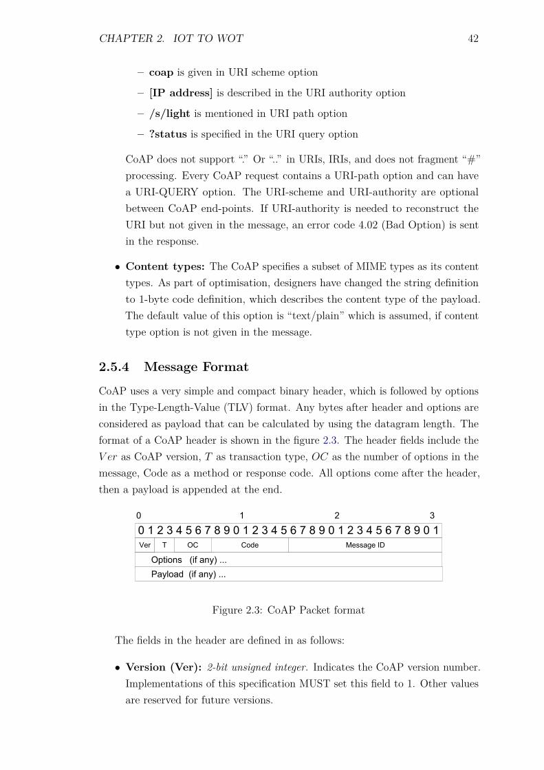
2.5.2 Methods . . . . . . . . . . . . . . . . . . . . . . . . . . . . . 402.5.3 Options . . . . . . . . . . . . . . . . . . . . . . . . . . . . . 412.5.4 Message Format . . . . . . . . . . . . . . . . . . . . . . . . . 422.5.5 UDP binding . . . . . . . . . . . . . . . . . . . . . . . . . . 442.5.6 Interaction Model . . . . . . . . . . . . . . . . . . . . . . . . 44
2.5.6.1 Synchronous response . . . . . . . . . . . . . . . . 442.5.6.2 Asynchronous response . . . . . . . . . . . . . . . . 46
2.5.7 Resource discovery . . . . . . . . . . . . . . . . . . . . . . . 462.5.8 Caching and Proxying . . . . . . . . . . . . . . . . . . . . . 47
2.6 Protocol Integration Approaches . . . . . . . . . . . . . . . . . . . . 472.6.1 Gateway approach . . . . . . . . . . . . . . . . . . . . . . . 472.6.2 Compression approach . . . . . . . . . . . . . . . . . . . . . 48
2.7 Technologies for Experiments . . . . . . . . . . . . . . . . . . . . . 482.7.1 Operating System: CONTIKI . . . . . . . . . . . . . . . . . 482.7.2 Simulator: COOJA . . . . . . . . . . . . . . . . . . . . . . . 49
2.8 Summary . . . . . . . . . . . . . . . . . . . . . . . . . . . . . . . . 50
3 Service Discovery (SD) in Literature 513.1 Introduction . . . . . . . . . . . . . . . . . . . . . . . . . . . . . . . 513.2 SD Objectives . . . . . . . . . . . . . . . . . . . . . . . . . . . . . . 513.3 SD Entities . . . . . . . . . . . . . . . . . . . . . . . . . . . . . . . 523.4 SD Classifications . . . . . . . . . . . . . . . . . . . . . . . . . . . . 523.5 Centralised architectures . . . . . . . . . . . . . . . . . . . . . . . . 53
3.5.1 SLP (Service Location Protocol) . . . . . . . . . . . . . . . . 533.5.2 SLP-based adaptations and optimised solutions . . . . . . . 543.5.3 JINI (Java Intelligent Network Interface) . . . . . . . . . . . 553.5.4 Salutation . . . . . . . . . . . . . . . . . . . . . . . . . . . . 563.5.5 FRODO (Framework for Robust and Resource-aware Dis-
covery) . . . . . . . . . . . . . . . . . . . . . . . . . . . . . . 563.5.6 SLEEPER . . . . . . . . . . . . . . . . . . . . . . . . . . . . 573.5.7 Splendor . . . . . . . . . . . . . . . . . . . . . . . . . . . . . 58
3.6 Distributed architectures . . . . . . . . . . . . . . . . . . . . . . . . 583.6.1 Domain Name Server (DNS) based . . . . . . . . . . . . . . 583.6.2 Clustering based . . . . . . . . . . . . . . . . . . . . . . . . 603.6.3 Hash-based P2P . . . . . . . . . . . . . . . . . . . . . . . . . 62
3.7 Directory-less architectures . . . . . . . . . . . . . . . . . . . . . . . 633.8 Cross-layer design . . . . . . . . . . . . . . . . . . . . . . . . . . . . 663.9 Discussion from 6LoWPAN’s perspective . . . . . . . . . . . . . . . 673.10 Service Discovery (SD) Process . . . . . . . . . . . . . . . . . . . . 71
CONTENTS 8
3.10.1 Service description . . . . . . . . . . . . . . . . . . . . . . . 723.10.2 Service advertisement/registration . . . . . . . . . . . . . . . 723.10.3 Service discovery . . . . . . . . . . . . . . . . . . . . . . . . 733.10.4 Service selection . . . . . . . . . . . . . . . . . . . . . . . . . 743.10.5 Service Invocation . . . . . . . . . . . . . . . . . . . . . . . 74
3.11 Challenges . . . . . . . . . . . . . . . . . . . . . . . . . . . . . . . . 753.11.1 Scalability . . . . . . . . . . . . . . . . . . . . . . . . . . . . 753.11.2 Energy, Memory and Bandwidth Constraints . . . . . . . . . 763.11.3 Reliability and accuracy . . . . . . . . . . . . . . . . . . . . 763.11.4 Heterogeneity and resource-awareness . . . . . . . . . . . . . 763.11.5 Security and privacy . . . . . . . . . . . . . . . . . . . . . . 76
3.12 New perspectives . . . . . . . . . . . . . . . . . . . . . . . . . . . . 773.12.1 Context Awareness . . . . . . . . . . . . . . . . . . . . . . . 773.12.2 Adaptability . . . . . . . . . . . . . . . . . . . . . . . . . . . 78
3.13 Summary and Discussion . . . . . . . . . . . . . . . . . . . . . . . . 79
4 Service Discovery for the IoT: A Requirement Analysis 804.1 Introduction . . . . . . . . . . . . . . . . . . . . . . . . . . . . . . . 804.2 Scenario . . . . . . . . . . . . . . . . . . . . . . . . . . . . . . . . . 804.3 User Interactions . . . . . . . . . . . . . . . . . . . . . . . . . . . . 824.4 IoT Service Discovery Requirements . . . . . . . . . . . . . . . . . . 82
4.4.1 Heterogeneity and Interoperability . . . . . . . . . . . . . . 834.4.2 Context-awareness . . . . . . . . . . . . . . . . . . . . . . . 834.4.3 Adaptability . . . . . . . . . . . . . . . . . . . . . . . . . . . 844.4.4 Constrained networks . . . . . . . . . . . . . . . . . . . . . . 84
4.5 Summary . . . . . . . . . . . . . . . . . . . . . . . . . . . . . . . . 85
5 A Context-aware Service Discovery Protocol (SDP) for the IoT 875.1 Introduction . . . . . . . . . . . . . . . . . . . . . . . . . . . . . . . 875.2 Architecture . . . . . . . . . . . . . . . . . . . . . . . . . . . . . . . 87
5.2.1 Directory Agent (DA) . . . . . . . . . . . . . . . . . . . . . 885.2.2 Service Agent (SA) . . . . . . . . . . . . . . . . . . . . . . . 895.2.3 User Agent (UA) . . . . . . . . . . . . . . . . . . . . . . . . 89
5.3 Communication Protocol . . . . . . . . . . . . . . . . . . . . . . . . 895.4 Service Description . . . . . . . . . . . . . . . . . . . . . . . . . . . 895.5 Context awareness . . . . . . . . . . . . . . . . . . . . . . . . . . . 905.6 Registration and Status maintenance . . . . . . . . . . . . . . . . . 93
5.6.1 Provision of the DA’s IP . . . . . . . . . . . . . . . . . . . . 935.6.2 Status maintenance . . . . . . . . . . . . . . . . . . . . . . . 94
CONTENTS 9
5.7 Service Discovery . . . . . . . . . . . . . . . . . . . . . . . . . . . . 945.8 Service Selection . . . . . . . . . . . . . . . . . . . . . . . . . . . . 955.9 Service Inovcation . . . . . . . . . . . . . . . . . . . . . . . . . . . . 985.10 Overall framework . . . . . . . . . . . . . . . . . . . . . . . . . . . 985.11 Message Formats . . . . . . . . . . . . . . . . . . . . . . . . . . . . 99
5.11.1 UPD (Update) for registration . . . . . . . . . . . . . . . . . 995.11.2 UPD (Update) message for Status maintenance . . . . . . . 1015.11.3 SDR (Service Discovery Request) . . . . . . . . . . . . . . . 102
5.12 Summary and Discussion . . . . . . . . . . . . . . . . . . . . . . . . 104
6 Experimental Design and Performance Metric 1066.1 Introduction . . . . . . . . . . . . . . . . . . . . . . . . . . . . . . . 1066.2 Performance Metrics . . . . . . . . . . . . . . . . . . . . . . . . . . 106
6.2.1 Control packet overhead . . . . . . . . . . . . . . . . . . . . 1066.2.2 Service Discovery Delay . . . . . . . . . . . . . . . . . . . . 1076.2.3 Service Invocation Delay and cache hits . . . . . . . . . . . . 1076.2.4 Energy Efficiency and Network lifetime . . . . . . . . . . . . 1086.2.5 Scalability factor: Packets to the DA . . . . . . . . . . . . . 1106.2.6 Reliability and Accuracy . . . . . . . . . . . . . . . . . . . . 110
6.3 Experimental Setup . . . . . . . . . . . . . . . . . . . . . . . . . . . 1116.3.1 Topology . . . . . . . . . . . . . . . . . . . . . . . . . . . . . 113
6.4 Experimental Design . . . . . . . . . . . . . . . . . . . . . . . . . . 1186.5 TRENDY’s Service Selection Experiments . . . . . . . . . . . . . . 120
6.5.1 Introduction . . . . . . . . . . . . . . . . . . . . . . . . . . . 1206.5.2 Control packet overhead . . . . . . . . . . . . . . . . . . . . 1206.5.3 Service Invocation Delay . . . . . . . . . . . . . . . . . . . . 1246.5.4 Energy Consumption and network lifetime . . . . . . . . . . 1276.5.5 Packets at the DA: a scalability factor . . . . . . . . . . . . 1296.5.6 Reliability and Accuracy . . . . . . . . . . . . . . . . . . . . 129
6.6 Summary and Discussion . . . . . . . . . . . . . . . . . . . . . . . . 130
7 Adaptive Reporting Timer 1317.1 Introduction . . . . . . . . . . . . . . . . . . . . . . . . . . . . . . . 1317.2 Aims . . . . . . . . . . . . . . . . . . . . . . . . . . . . . . . . . . . 1317.3 Adaptive Timer Process . . . . . . . . . . . . . . . . . . . . . . . . 132
7.3.1 Design . . . . . . . . . . . . . . . . . . . . . . . . . . . . . . 1327.3.2 Example Scenario . . . . . . . . . . . . . . . . . . . . . . . . 135
7.4 Message Formats . . . . . . . . . . . . . . . . . . . . . . . . . . . . 1377.4.1 Updated TRENDY reporting message . . . . . . . . . . . . 137
CONTENTS 10
7.5 Experiments and Results . . . . . . . . . . . . . . . . . . . . . . . . 1387.5.1 Introduction . . . . . . . . . . . . . . . . . . . . . . . . . . . 1387.5.2 Control packet overhead . . . . . . . . . . . . . . . . . . . . 1397.5.3 Energy Consumption and network lifetime . . . . . . . . . . 1447.5.4 Scalability factor: Packets to the DA . . . . . . . . . . . . . 1487.5.5 Service Invocation Delay . . . . . . . . . . . . . . . . . . . . 1507.5.6 Reliability and Accuracy . . . . . . . . . . . . . . . . . . . . 152
7.6 Summary and Discussion . . . . . . . . . . . . . . . . . . . . . . . . 152
8 Context-aware Grouping 1548.1 Introduction . . . . . . . . . . . . . . . . . . . . . . . . . . . . . . . 1548.2 Aims . . . . . . . . . . . . . . . . . . . . . . . . . . . . . . . . . . . 1548.3 Architecture . . . . . . . . . . . . . . . . . . . . . . . . . . . . . . . 155
8.3.1 Group Member (GM) . . . . . . . . . . . . . . . . . . . . . . 1558.3.2 Group Leader (GL) . . . . . . . . . . . . . . . . . . . . . . . 155
8.4 Grouping Process . . . . . . . . . . . . . . . . . . . . . . . . . . . . 1568.5 Best GL Selection . . . . . . . . . . . . . . . . . . . . . . . . . . . . 1598.6 Message Formats . . . . . . . . . . . . . . . . . . . . . . . . . . . . 159
8.6.1 UPD (Update) for GL registration . . . . . . . . . . . . . . 1598.6.2 Grouping Messages . . . . . . . . . . . . . . . . . . . . . . . 160
8.6.2.1 YGM (Your Group member) . . . . . . . . . . . . 1608.6.2.2 RGM (Remove Group member) . . . . . . . . . . . 1618.6.2.3 YGL (Your Group Leader) . . . . . . . . . . . . . 162
8.6.3 Reporting Messages . . . . . . . . . . . . . . . . . . . . . . . 1638.6.3.1 UPD (Update) message for Status maintenance . . 1638.6.3.2 NRP (Not reported) . . . . . . . . . . . . . . . . . 1638.6.3.3 SSC (Some Service Changed) . . . . . . . . . . . . 1648.6.3.4 GLD (Group Leader Done) . . . . . . . . . . . . . 165
8.6.4 Discovery Messages . . . . . . . . . . . . . . . . . . . . . . . 1668.6.4.1 FWD (Forward Query) . . . . . . . . . . . . . . . . 167
8.7 Experiments: Group Scalability . . . . . . . . . . . . . . . . . . . . 1688.7.1 Introduction . . . . . . . . . . . . . . . . . . . . . . . . . . . 1688.7.2 Control packet overhead . . . . . . . . . . . . . . . . . . . . 1718.7.3 Energy Consumption and network lifetime . . . . . . . . . . 1738.7.4 Scalability factor: Packets to the DA . . . . . . . . . . . . . 1758.7.5 Service Invocation Delay . . . . . . . . . . . . . . . . . . . . 1768.7.6 Reliability and Accuracy . . . . . . . . . . . . . . . . . . . . 178
8.8 Experiments: Grouping with different groups . . . . . . . . . . . . . 1788.8.1 Introduction . . . . . . . . . . . . . . . . . . . . . . . . . . . 178
CONTENTS 11
8.8.2 Control packet overhead . . . . . . . . . . . . . . . . . . . . 1798.8.3 Energy Consumption and network lifetime . . . . . . . . . . 1818.8.4 Scalability factor: Packets to the DA . . . . . . . . . . . . . 1838.8.5 Service Invocation Delay . . . . . . . . . . . . . . . . . . . . 1858.8.6 Reliability and Accuracy . . . . . . . . . . . . . . . . . . . . 186
8.9 Summary and Discussion . . . . . . . . . . . . . . . . . . . . . . . . 186
9 Adaptive Piggybacked Publishing (APPUB): An Algorithm forAdaptive Caching 1879.1 Introduction . . . . . . . . . . . . . . . . . . . . . . . . . . . . . . . 1879.2 Aims . . . . . . . . . . . . . . . . . . . . . . . . . . . . . . . . . . . 1879.3 Design . . . . . . . . . . . . . . . . . . . . . . . . . . . . . . . . . . 188
9.3.1 APPUB Process . . . . . . . . . . . . . . . . . . . . . . . . . 1889.3.2 DA’s role . . . . . . . . . . . . . . . . . . . . . . . . . . . . 1899.3.3 SA’s role . . . . . . . . . . . . . . . . . . . . . . . . . . . . . 1899.3.4 Cache Format . . . . . . . . . . . . . . . . . . . . . . . . . . 191
9.4 Message Format . . . . . . . . . . . . . . . . . . . . . . . . . . . . . 1919.4.1 Update for TRENDY’s UPD reporting message . . . . . . . 191
9.5 Experiments and Results . . . . . . . . . . . . . . . . . . . . . . . . 1929.5.1 Introduction . . . . . . . . . . . . . . . . . . . . . . . . . . . 1929.5.2 Service Invocation Delay and Cache hits . . . . . . . . . . . 1939.5.3 Energy Consumption and network lifetime . . . . . . . . . . 1989.5.4 Control packet overhead . . . . . . . . . . . . . . . . . . . . 2019.5.5 Scalability factor: Packets to the DA . . . . . . . . . . . . . 2049.5.6 Reliability and Accuracy . . . . . . . . . . . . . . . . . . . . 204
9.6 Summary and Discussion . . . . . . . . . . . . . . . . . . . . . . . . 204
10 TRENDY: a Trend-based Service Discovery Solution for the IoT20610.1 Introduction . . . . . . . . . . . . . . . . . . . . . . . . . . . . . . . 20610.2 TRENDY Protocol with Adaptive Techniques . . . . . . . . . . . . 206
10.2.1 Message Format . . . . . . . . . . . . . . . . . . . . . . . . . 20610.2.2 SA roles . . . . . . . . . . . . . . . . . . . . . . . . . . . . . 20710.2.3 Policies . . . . . . . . . . . . . . . . . . . . . . . . . . . . . 20710.2.4 Framework . . . . . . . . . . . . . . . . . . . . . . . . . . . 207
10.3 Experiments and results . . . . . . . . . . . . . . . . . . . . . . . . 20810.3.1 Introduction . . . . . . . . . . . . . . . . . . . . . . . . . . . 20810.3.2 Service Invocation Delay and Cache hits . . . . . . . . . . . 20910.3.3 Control packet overhead . . . . . . . . . . . . . . . . . . . . 21110.3.4 Scalability factor: Packets to the DA . . . . . . . . . . . . . 213
CONTENTS 12
10.3.5 Energy Consumption and Network Lifetime . . . . . . . . . 21510.3.6 Memory Requirements . . . . . . . . . . . . . . . . . . . . . 218
10.4 Summary and Discussion . . . . . . . . . . . . . . . . . . . . . . . . 219
11 Comparison with other solutions 22111.1 Introduction . . . . . . . . . . . . . . . . . . . . . . . . . . . . . . . 22111.2 Context-awareness . . . . . . . . . . . . . . . . . . . . . . . . . . . 22211.3 Extensibility . . . . . . . . . . . . . . . . . . . . . . . . . . . . . . . 22211.4 Interoperability . . . . . . . . . . . . . . . . . . . . . . . . . . . . . 22311.5 Constraints Considerations . . . . . . . . . . . . . . . . . . . . . . . 22311.6 Dependencies . . . . . . . . . . . . . . . . . . . . . . . . . . . . . . 22411.7 Performance Metrics . . . . . . . . . . . . . . . . . . . . . . . . . . 224
11.7.1 Service Discovery delay . . . . . . . . . . . . . . . . . . . . . 22411.7.2 Service Invocation support . . . . . . . . . . . . . . . . . . . 22411.7.3 Scalability . . . . . . . . . . . . . . . . . . . . . . . . . . . . 22511.7.4 Energy Consumption . . . . . . . . . . . . . . . . . . . . . . 226
11.8 Summary . . . . . . . . . . . . . . . . . . . . . . . . . . . . . . . . 226
12 Conclusions and Future Work 22812.1 Conclusions . . . . . . . . . . . . . . . . . . . . . . . . . . . . . . . 22812.2 Future Work . . . . . . . . . . . . . . . . . . . . . . . . . . . . . . . 231
References 232
Appendices 246
A Automation of experiments 247A.1 Scenarios automation . . . . . . . . . . . . . . . . . . . . . . . . . . 247A.2 Script for 6LoWPAN data gathering . . . . . . . . . . . . . . . . . 253
B Logs for validation and debugging 258B.1 Simulation Log . . . . . . . . . . . . . . . . . . . . . . . . . . . . . 258B.2 COOJA Log . . . . . . . . . . . . . . . . . . . . . . . . . . . . . . . 262
B.2.1 Case-x-packet.pcap . . . . . . . . . . . . . . . . . . . . . . . 262B.2.2 Lowpan-detail.log . . . . . . . . . . . . . . . . . . . . . . . . 262B.2.3 l-energy-all.log . . . . . . . . . . . . . . . . . . . . . . . . . 265B.2.4 l-energy-ind.log . . . . . . . . . . . . . . . . . . . . . . . . . 266B.2.5 l-packet-all.log . . . . . . . . . . . . . . . . . . . . . . . . . . 267B.2.6 l-packet-ind.log . . . . . . . . . . . . . . . . . . . . . . . . . 268
B.3 DA Log . . . . . . . . . . . . . . . . . . . . . . . . . . . . . . . . . 269B.3.1 daperformance.log . . . . . . . . . . . . . . . . . . . . . . . 269

CONTENTS 13
B.3.2 da-detail.log . . . . . . . . . . . . . . . . . . . . . . . . . . . 269B.3.3 daFullDetail.log . . . . . . . . . . . . . . . . . . . . . . . . . 272
B.4 UA Log . . . . . . . . . . . . . . . . . . . . . . . . . . . . . . . . . 274B.4.1 uaperformance-processed.log . . . . . . . . . . . . . . . . . . 274B.4.2 ua-detail.log . . . . . . . . . . . . . . . . . . . . . . . . . . . 275
C Automation for statistics processing and graph generation 276C.1 Data Processing . . . . . . . . . . . . . . . . . . . . . . . . . . . . . 276C.2 GNUPLOT graphs generation . . . . . . . . . . . . . . . . . . . . . 284
Acronyms
6LoWPAN IPv6 over Low power Wireless Personal Area Networks
ACK Acknowledgement
AES Advanced Encryption Standard
AODV Ad-hoc On-Demand Distance Vector Routing
APPUB Adaptive Piggybacked Publishing
BXML Binary XML
CoAP Constrained Application Protocol
CoRE Constrained RESTful Environments
CSMA Carrier Sense Multiple Access
DA Directory Agent
DAO DODAG Advertisement Object
DHCP Dynamic Host Configuration Protocol
DIO DODAG Information Object
DIS DODAG Information Solicitation
DNS Domain Name System
DODAG Destination Oriented Directed Acyclic Graph
EUI-64 64-bit Extended Unique Identifier
EXI Efficient XML Interchange
FWD Forward Query
14

Acronyms 15
GL Group Leader
GLD Group Leader Done
GM Group Member
HTTP Hyper Text Terminal Protocol
IETF Internet Engineering Task Force
IoT Internet of Things
IS-IS Intermediate System to Intermediate System
LLN Low Power and Lossy Network
M2M Machine-to-Machine
MAC Medium Access Control
MANET Mobile Ad-hoc Network
MIME Multipurpose Internet Mail Extensions
MTU Maximum transmission unit
NAPTR Name Authority Pointer
NRP Not Reported
OF Objective Function
OGC Open Geospatial Consortium
OLSR Optimized Link State Routing Protocol
OSPF Open Shortest Path First
PubSub Publish and Subscribe
QoS Quality of Service
RDC Radio Duty Cycling
RDF Resource Description Framework
REST Representational state transfer
Acronyms 16
RESTful Representational state transfer based
RGM Remove Group Member
RPC Remote Procedure Call
RPL IPv6 Routing Protocol for Low power and Lossy Networks
RQL RDF Query Language
RTCP RTP Control Protocol
RTP Real-time Transport Protocol
SA Service Agent
SD Service Discovery
SDP Service Discovery Protocol
SDR Service Discovery Request
SIP Session Initiation Protocol
SLIP Serial Line Internet Protocol
SOAP Simple Object Access Protocol
SSC Some Service Changed
SSDP Simple Service Discovery Protocol
TCP Transport Control Protocol
TRENDY Trend-based Service Discovery Protocol (Proposed Solution)
UA User Agent
UDP User Datagram Protocol
UPD Update
uPnP Universal Plug and Play
WADL Web Application Description Language
WBXML WAP Binary XML
WoT Web of things

Acronyms 17
WSDL Web Service Description Language
WSN Wireless Sensor Network
WSNs Wireless Sensor Networks
YGL Your Group Leader
YGM Your Group Member
Chapter 1
Introduction
The IoT vision has drastically changed the way we foresee the future Internet [10].Integration of constrained networks with the broader Internet can open new avenuesfor these networks, as this extends the ability of these networks to share resourcesand information with other networks. These low cost, battery operated deviceswith limited data rates are becoming smarter and making this kind of integrationmore feasible.
Arrival of new standards has allowed constrained networks to integrate seam-lessly with the Internet. IP-based devices can be connected easily to other IPnetworks, without the need for complex translation gateways. This gives theopportunity for the reusability of existing infrastructure and proven standards,instead of using proprietary solutions. Moreover, IP connectivity enables WSNsto utilise the broad body of existing IP tools and standards such as firewalls,proxies, caches. Furthermore, the use of IP outperforms existing systems in averageduty-cycle, per-hop latency, and data reception rate with a higher traffic load [56].However, the inherent nature of these networks still poses many challenges inadapting existing IP-based standards.
Devices can offer their functionalities by abstracting them as services. Moreover,the provision of Service Discovery (SD) and service selection can assist the userapplications to find the required services. This changes the traditional view ofthese constrained networks by making them directly accessible over the Internet.Furthermore, web services can provide a standard interface to offer interoperabilitywith other existing similar solutions. However, the design of such a solution facesthe underlying issues of these networks, for example, small packet size and sleepcycles. In constrained environments, services are mostly hosted on battery operateddevices, which can fail without any notification. Thus, these networks require anefficient, reliable and interoperable solution for SD. This research project analysesexisting solutions with the IoT requirements and challenges of its constraineddomains, to identify the potential gaps. Consequently, the project proposes a
18
CHAPTER 1. INTRODUCTION 19
compact, adaptive and context-aware SD solution that considers the inherentchallenges, and offers the desired features to encompass them.
This chapter highlights the significance of the research problems and relatedchallenges, and then summarises the original contributions made by this project.
1.1 Motivation
The Internet Engineering Task Force (IETF)’s 6LoWPAN [93] standard has madeit possible for constrained networks to connect directly to the Internet. Thisintegration has opened new horizons for these devices. Recent developments havechanged the profile of WSNs from isolated and application-specific, to more in-terconnected and directly accessible 6LoWPANs. However, these networks stillhave constrained properties, including limited packet size, intermittent communic-ation, high packet loss, restricted power and throughput. Besides these challenges,the major benefit of integration is resource sharing, which can be achieved byabstracting the resources as services. A service can provide any data reading ormeasurement such as temperature reading of a sensor, which can be shared insidea 6LoWPAN or with external IP network. Services can be further composed tocreate higher-level services. Furthermore, mashups can be generated to providenew functionality with the combination of different services [136]. To make use ofall potential benefits; discovery of available services is highly crucial and demandssuitable SD, and selection solution.
The employment of existing IP-based SD solutions is a first choice to enablethe inherent interoperability. However, the large packet sizes and heavy controloverhead of these solutions make these infeasible for constrained networks such as6LoWPANs. The difference of both networks can be understood by their Maximumtransmission unit (MTU), which is 1280 bytes for IPv6 and is only 127 bytes for6LoWPAN (which uses IEEE 802.15.4). This implies that even in the case of singleIPv6 packet transmission, a 6LoWPAN network needs to send multiple packets,which will entail heavy traffic load and bandwidth utilisation. Similarly otheravailable distributed solutions demand excessive use of broadcast or multicast,which is unsuitable in networks with devices with sleep cycles and intermittentconnectivity.
A 6LoWPAN based network mostly consists of heterogeneous devices; therefore,a solution should be able to deal with the heterogeneity. Web services offer thesolution with high interoperability, customisation and flexibility by providing astandard interface to services. These characteristics make web services a keytechnology to enable WoT vision that depicts a view where a collection of webservices that could be discovered, composed and executed [136]. Although web
CHAPTER 1. INTRODUCTION 20
services remarkably change the way how services are accessed, but are a poor matchfor constrained networks because of the inherent complexity [114]. Both SimpleObject Access Protocol (SOAP) based big web services, and Representationalstate transfer (REST) in their traditional forms are impractical for such networks.However, constrained nodes can benefit from IETF’s CoAP [13] standard, whichoffers compact and optimised RESTful web services.
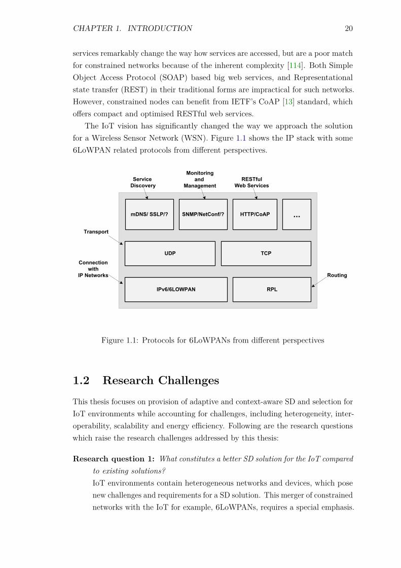
The IoT vision has significantly changed the way we approach the solutionfor a Wireless Sensor Network (WSN). Figure 1.1 shows the IP stack with some6LoWPAN related protocols from different perspectives.
����� ������ ���� � ���
��� ��
���������� � ���
��������������
���������������
���������!"�#
�"�"!������$��%&
��' ��������
�"��(���
����������)��*
�� ���)��+� ��%���!
Figure 1.1: Protocols for 6LoWPANs from different perspectives
1.2 Research Challenges
This thesis focuses on provision of adaptive and context-aware SD and selection forIoT environments while accounting for challenges, including heterogeneity, inter-operability, scalability and energy efficiency. Following are the research questionswhich raise the research challenges addressed by this thesis:
Research question 1: What constitutes a better SD solution for the IoT comparedto existing solutions?IoT environments contain heterogeneous networks and devices, which posenew challenges and requirements for a SD solution. This merger of constrainednetworks with the IoT for example, 6LoWPANs, requires a special emphasis.

CHAPTER 1. INTRODUCTION 21
Thus, a review of existing SD solutions is required in the context of thesechallenges.
• Literature review of existing SD solutions: A critical analysis of existingSD solutions and discussion of their applicability for constrained domainsis required to find out the research gaps and to take better designdecisions.
• The IoT requirements for a SD: Clear understanding of the new IoTperspective is needed to be analysed in the context of future scenarios.The general and constrained network specific SD requirements andchallenges are needed to be scrutinised and well defined.
Research question 2: How IP-based WSNs consisting of resource-constrainednodes can offer efficient and interoperable SD and selection to user applica-tions in the IoT?New technologies have enabled WSNs to integrate with the Internet, butwork still needed to make them an active part of the web. The discoveryof the available services in a WSN is important to access the functionalitywithin a dynamic environment. Therefore, the mechanism for discovery ofservices is essential to assist the user to discover required services. A userapplication query for SD can result in a list of matching services, even though,application actually looking for one appropriate service. A SDP should ad-dress this requirement by offering context-aware service selection as this is anorm in IoT scenarios. A discovery depending on multicast or broadcast isnot an efficient choice in terms of efficiency and sometimes error prone innetworks with intermittent connectivity. Consequently, challenge is to designan interoperable SD and selection solution that satisfy the requirements ofthe IoT, while providing the required efficiency to meet the challenges posedby constrained nodes and networks.
• Interoperability: Web service interface is always preferable to allowthe desired interoperability in the IoT; however, the challenge is toenable this paradigm for its constrained domains. The WoT vision hasrecommended the use of RESTful web services as a standard interfacefor the services hosted by smart devices [43]. However, offering theweb service interface using traditional solutions put more burden onconstrained nodes, and is not feasible for many low capacity nodes andnetworks.
Research question 3: How a SD solution can become context-aware and enableservice composition without creating heavy traffic load on the network?
CHAPTER 1. INTRODUCTION 22
The IoT user applications can look for one best service to issue queries orto execute a command on a collection of nodes sharing some context (forexample, switching the actuators on in some area). The nodes in a WSN existin an environment where collaboration between them can reduce the overhead,and consequently, enable the creation of new high-level services. However,the challenge is to enable such a functionality in new IoT paradigm withdiverse networks that have constraints. The SD solution needs to find thosecommon context attributes before applying some mechanism to collectivelyinvoke services. The collection of context information and approach to enableservice composition should be efficient for constrained domains of the IoT.
Research question 4: How to deal with mostly unavailable nodes (because ofsleep cycles) and high number of service invocations by the users?Energy is a precious resource for constrained wireless sensor nodes; therefore,these nodes use different Radio Duty Cycling (RDC) algorithms to saveenergy. Furthermore, IP-based WSNs offer services to the broad range ofusers and applications, so there is a potential for an overwhelming number ofrequests. The sheer number of requests face more delays when nodes keep onsleeping for most of the time, and consequently more energy is consumed bydevices in a multi-hop network. The question arises that how this trade-offof energy conservation and better user response can be managed.
1.3 Aims and Objectives
The main aim of this research project is to design a compact SD solution for theIoT with low control overhead, minimised energy consumption and reduced SDand invocation delay. New technologies, including, 6LoWPAN, are shifting theexisting paradigm of the Internet by allowing resource-constrained networks tobecome an active part of the IoT. The target of this work is to analyse and coverthe new challenges for SD posed by this new paradigm. However, these networksand devices are still resource-constrained and require an efficient and compact SDP.The solution needs to balance the trade-off of interoperability and efficiency whileensuring its applicability for a wide variety of networks in the IoT. The objectivesof this research project are:
• To investigate the SD process and scrutinise design options available atdifferent stages.
• To explore existing SDPs in literature, categorise them and examine theirfeatures.
CHAPTER 1. INTRODUCTION 23
• To scrutinise existing research efforts for providing SD for 6LoWPANs, andthe research gaps left by those schemes.
• To investigate the SD requirements for the IoT in context of some use-casescenarios, so the design of proposed protocol can cover new challenges.
• To design and test new SD solution that:
1. has open and extensible framework to address the diverse capabilities ofthe networks in the IoT.
2. should consider interoperability with an existing approach.
3. should address new requirements posed by the IoT.
4. should allow context-aware SD by allowing sophisticated queries.
5. should provide context-aware service selection to assist user applicationsfor choosing more efficient hosts.
6. is independent of underlying protocols at different layers, including,routing, Medium Access Control (MAC) and RDC etc.
7. should have compact implementation and message sizes.
8. is efficient in terms of control overhead, energy consumption and SDand invocation delay.
9. should be adaptive to network dynamics, so can provide better userresponse even during high demand.
10. should provide reliable and accurate information, including, serviceinformation and cached values.
11. is scalable, by conforming that the control overhead is not proportionalto increasing number of devices.
1.4 Research Methodology
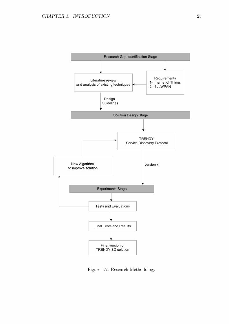
Research gap identification is the first stage of this work, which consists of literaturereview and new IoT requirements gathering. Firstly, the concepts related toemerging IoT environments are developed to identify the basic requirements andchallenges posed by its constrained sub-domains. This is followed by an extensiveliterature review to analyse existing SD protocols. The protocols are categorisedand then scrutinised for different stages of SD. The identified IoT SD requirementsare used in the scrutiny. The design guidelines is the outcome of this stage for theconception of a better design for new solution.

CHAPTER 1. INTRODUCTION 24
The solution design stage proposes a solution to achieve the objectives (Sec-tion 1.3) according to the design guidelines produced in the first stage. The protocolis implemented and tested in the experiments stage. The results of the evaluationare fed back to the design stage to tackle the unsolved issues. Consequently,new algorithms are devised to improve the solution and to make it more feasible,efficient and suitable for IoT environments. These algorithms are integrated withthe existing solution and tested individually. The generated results are used toimprove the proposed mechanisms. Finally, the solution composed of all algorithmsis tested, verified and validated at experiments stage before finalising the designstage. Figure 1.2 illustrates all stages in a simplified flowchart.
CHAPTER 1. INTRODUCTION 25
�������� �� ��� ����� ��� � ���
�� ��� ��� ��������� �������� �� ���� ��� ���������
���������� ��� � ���� �� ������ � !��"#$%
���� ��� &����� � ���
��'%&(������� &�������� #�� ����
'������� � � ���
%�� $����� �� � ������ ���� ���
)���� ��� � ��� ����� �
)���� ������� ����'%&( �& ���� ���
&���������������
������� �
��� � ��� '����� ����
Figure 1.2: Research Methodology
CHAPTER 1. INTRODUCTION 26
1.5 Original Contributions
In this section, the main contributions of this thesis are described with regard tothe posed research questions and challenges.
Contribution 1: Analysed SD requirements for the IoTThe demands of IoT environments are very diverse. However, to devise abetter solution a review of existing solutions is needed by focusing on therequirements of IoT and its constrained sub-domain. At first, Chapter 2covers the detail of IoT environments by explaining related technologies.Subsequently, a literature review of existing SD solutions in context of6LoWPANs is conducted in Chapter 3. This chapter also discusses the detailsof general challenges and new perspectives in context of SD. Furthermore,Chapter 4 describes some IoT use case scenarios and emphasises the generalIoT and specific 6LoWPAN requirements for SD.
Contribution 2: Proposed a SD and selection solution for IP-based Wirelesssensor networksThis project proposes TRENDY, a context-aware SD and selection solutionfor IP-based WSNs (Chapter 5), which uses the context information ofnodes to select the best matched service. Its service selection mechanismis evaluated in different experiments using different RDCs and topologies(Section 6.5). Moreover, CoAP is employed as a communication protocol thatenables the web service paradigm to provide service invocation and desiredinteroperability.
Contribution 3: Proposed an adaptive timer to reduce control overheadAn adaptive timer technique is proposed (Chapter 7) to minimise the overheadof status maintenance. It uses the service popularity (number of times aservice is discovered in a time window) as criteria to adaptively increaseor decrease the interval between status updates. The timer mechanism isevaluated in the number of experiments using different number of nodes andtopologies.
Contribution 4: Proposed a grouping technique to provide scalable architectureand to enable service compositionChapter 8 covers the detail of a grouping approach, which uses the contextinformation to group nodes. It creates an application-level overlay of thenetwork to localise the status maintenance and provide basis to enableservice composition while localising the traffic within a group. It makesthe solution resource-aware by defining distinctive roles, which consist of
CHAPTER 1. INTRODUCTION 27
different modular features to deal with the heterogeneity. This allows nodesto implement different level of functionality depending on their capabilities.An evaluation is done to analyse the impact of grouping w.r.t. the size of agroup, and the number of groups in a network.
Contribution 5: Proposed adaptive caching technique to deal with sleepy nodesAn adaptive caching technique is proposed by this research project (Chapter 9)that reduces the burden on network’s bandwidth and delay in service invoca-tions. This technique helps the nodes to deal with the high number of servicerequests while conserving energy with sleep cycles. Furthermore, it’s cachepublishing ensures that the delay of service invocations tend to zero whenthe number of request increases drastically. This technique is evaluated usingdifferent network loads, RDCs and topologies.
1.6 Thesis structure
This thesis begins with the introduction of those technologies that have enabledconstrained networks to become an active part of the Internet. Chapter 2 introducesthe technologies needed to merge WSNs with the Internet. This chapter coversthe discussion of existing application protocol paradigms and their integrationin constrained networks to enable the WoT paradigm. Chapter 3 introduces therole of SD by explaining its objectives and entities. The literature is reviewed inthis chapter, by classifying existing SDPs by architectural design. Furthermore, itcovers the related issues and some new perspectives in the SD domain. Chapter 4presents the IoT SD requirements in the context of different future scenarios withan emphasis to 6LoWPANs. Chapter 5 describes the SD and selection solutionproposed by this research project. This chapter discusses the design details ofthe protocol, including aims, architecture, and protocol’s overview. The protocolspecifications including details of algorithms and message formats are also explainedin this chapter. Chapter 6 presents the experimental tools, performance metrics,experimental setup and design for evaluation of the solutions. It also coversthe evaluation of the service selection mechanism of TRENDY. Chapters 7, 8and 9 present the detail of three proposed techniques: adaptive reporting timer,context-aware grouping and adaptive caching. These chapters cover the detail ofdesign, performed experiments and generated results of the respected techniques.Chapter 10 combines the four contributions together to form an adaptive andcontext-aware SD solution for the IoT. This chapter also discusses the experimentsperformed and generated results by combining different techniques. The proposedsolution is then compared with some existing SD solutions in Chapter 11. The

CHAPTER 1. INTRODUCTION 28
thesis is concluded with the discussion of the research project’s contributions andfuture work in Chapter 12.
Chapter 2
From the Internet of Things (IoT)to the Web of Things (WoT)
2.1 Introduction
The IoT vision extends the current Internet to previously unconnected physicalthings. These everyday objects are connected to the virtual world and empowerremote users to control them. This paradigm transforms the computing trulyubiquitous - an idea coined by Mark Weiser [131]. New technologies have made thisintegration a reality by enabling even very low capable devices and isolated WSNsto become an active part of the Internet. The WoT [42] paradigm extends thisintegration to the application layer [45]. This chapter explains the technologies,which enable constrained networks to become the part of the Web. The detailsof different application protocol paradigms and related protocols are covered inthis chapter. In the end, it describes the employed technologies by this researchproject for implementation and evaluation.
2.2 6LoWPAN (IPv6 over Low power WirelessPersonal Area Networks)
6LoWPAN [90] is an IPv6 adaptation layer that defines mechanisms to connectresource constrained devices with IP [76]. These devices mostly communicate overlow power, lossy links such as IEEE 802.15.4. It uses a compression format [55] tocompress the IPv6 packets. The adaptation layer is introduced at the edge router,for translation of packets to and from IPv6 network.
A 6LoWPAN consists of one or many stub networks. A stub network is asmall network to which packets can be sent or received, but it doesn’t behave asa transit to other networks. The connection to other IP networks is maintained
29
CHAPTER 2. IOT TO WOT 30
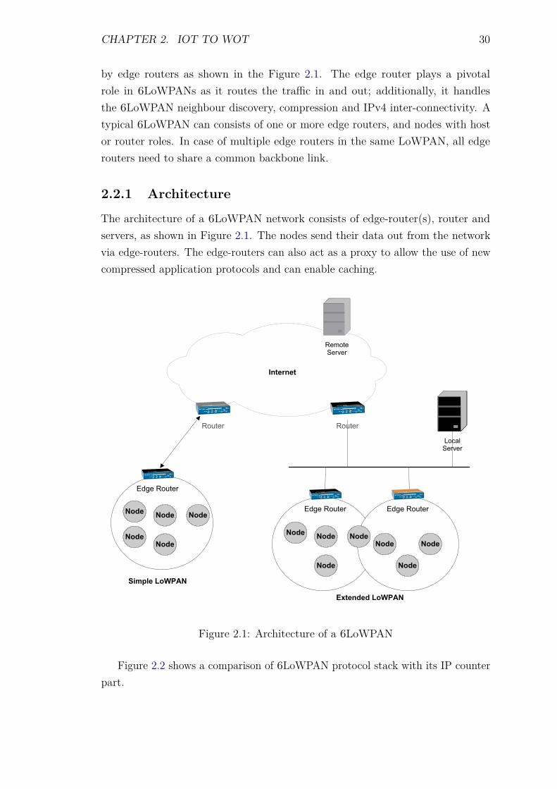
by edge routers as shown in the Figure 2.1. The edge router plays a pivotalrole in 6LoWPANs as it routes the traffic in and out; additionally, it handlesthe 6LoWPAN neighbour discovery, compression and IPv4 inter-connectivity. Atypical 6LoWPAN can consists of one or more edge routers, and nodes with hostor router roles. In case of multiple edge routers in the same LoWPAN, all edgerouters need to share a common backbone link.
2.2.1 Architecture
The architecture of a 6LoWPAN network consists of edge-router(s), router andservers, as shown in Figure 2.1. The nodes send their data out from the networkvia edge-routers. The edge-routers can also act as a proxy to allow the use of newcompressed application protocols and can enable caching.
������������
���������
�� ���
��������
����
������������
����
����
���� �� ���
��������
����
����
�� ���
��������
���� �� ���
���� ������
�������� ������
���� �� ���
Figure 2.1: Architecture of a 6LoWPAN
Figure 2.2 shows a comparison of 6LoWPAN protocol stack with its IP counterpart.

CHAPTER 2. IOT TO WOT 31
�����������
��������
������
���� ����
��������
�������� ��������� ���
���� ���
������� ���
�� �������� �����
������� ���� ��
���
�������� ��������� ���
�� ���
��������
������ �������� �����
����������� ����� ���
�� !��" �#$%�$����
Figure 2.2: IP and 6LoWPAN protocol stacks
2.2.2 Design Considerations
This section describes number of design considerations, which should be taken intoaccount while designing an application protocol for 6LoWPANs [112].
Link layer: 6LoWPANs use the IEEE 802.15.4 low power radio technology forwireless communication. This radio is quite distinctive in nature from IEEE802.11 WLANs, so the unlike attributes of IEEE 802.15.4 are highly con-siderable. It uses Carrier Sense Multiple Access (CSMA) as a MAC withmultiple retransmission. The rate of packet loss also increases if there is radiointerference. There is no built-in multi-cast support, which can be crucialin the context of sensor networks. Furthermore, links are asymmetrical, sothe packets successfully sent in one direction do not guarantee delivery fromthe other side. The most constraint feature of IEEE 802.15.4 is its limitedbandwidth as at the physical layer payload size is 127 bytes and offer only60-80 bytes ideally for a User Datagram Protocol (UDP) payload [114]. Thedata rates are also typically between 20 and 250 kbit/s and are shared byall nodes on the channel, and will drop further over multi-hops. Therefore,end-to-end reliability is important for applications, because of the lossy links.The application protocol for 6LoWPANs should use compact binary headersand payload formats.
Networking: UDP has the most favourable qualities (for example, connection-lessbehaviour) to be considered for 6LoWPANs. On the other hand, TransportControl Protocol (TCP) does have some use, but this will require a newenhanced, and compact version of TCP. This option is interesting to beconsidered as most of the IP-based protocols rely on TCP because of its
CHAPTER 2. IOT TO WOT 32
reliable connection-oriented byte stream. Large packet transfer can beachieved by using the fragmentation feature of 6LoWPAN, but this willincrease the traffic and message response time.
Host Identification Issues: The identification of the devices is a key for end-to-end communication. There are several ways in which a device can beidentified such as a serial number, the IPv6 number of node, 64-bit ExtendedUnique Identifier (EUI-64) number, or by its domain name. The IPv6 addresscan change for a mobile device when it moves or point of attachment changes.An EUI-64 [52] is a unique serial number of the device; it is reliable identifierbut needs to be resolved by the node.
Compression: Traditional IP protocols are not designed for constrained envir-onments; therefore, these do not address the inherent challenges in theseenvironments. For example, features like human readability and protocolextensibility are not of great priority in Machine-to-Machine (M2M) commu-nication. Similarly, constrained devices are not able to implement complexprotocols. Consequently, existing IP-based protocols require compression tobe applicable for constrained devices and environments.
Security: 6LoWPANs use link layer encryption for securing the links in a net-work. IEEE 802.15.4 also secures each link with a built-in 128 bit AdvancedEncryption Standard (AES) encryption feature. In a multi-hop network,intermediate hops to have the same encryption key, which makes the applica-tion data vulnerable on these hops. Applications that deal with importantdata demand more security, for example, enterprise and defence systems. Ifan application is dealing with sensitive data, it can apply end-to-end applica-tion layer security. This enables only the involved end-points to encrypt anddecrypt the data accurately.
2.3 RPL (IPv6 Routing Protocol for Lowpower and Lossy Networks)
IPv6 Routing Protocol for Low power and Lossy Networks (RPL) [133] is anIETF standard and focused on Low Power and Lossy Network (LLN) a class ofnetwork in which devices including routers have constraints on memory, processingpower and energy (battery powered). Furthermore, the types of traffic flows inthese networks include point-to-point (between devices inside a network), point-to-multipoint (from a central control point to a subset of devices inside a network),and multipoint-to-point (from devices inside a network towards a central control
CHAPTER 2. IOT TO WOT 33
point). In the start, the designers of RPL identified the routing requirements forLLNs, which were used to evaluate existing protocols including Open Shortest PathFirst (OSPF), Ad-hoc On-Demand Distance Vector Routing (AODV), IntermediateSystem to Intermediate System (IS-IS) and Optimized Link State Routing Protocol(OLSR). However, they couldn’t find a match for the unique requirements of LLNssuch as constrained devices and unreliable lossy links with high loss rates, low datarates, and instability. Subsequently, RPL was designed that is tailored to deal withthe requirements of wide range of LLN application domains.
2.3.1 Protocol and Topology Construction
RPL is a proactive distance vector protocol and does not rely on any particularfeatures of a specific link layer mechanism. It requires bi-directional links (mayhave asymmetric properties) between devices to build one or more DestinationOriented Directed Acyclic Graph (DODAG). A DODAG is a set of vertices withoutany cycle in them where each node has a path towards a single root. All theroutes are optimised for traffic to or from the root that represents the sink for thetopology. This makes RPL more suitable for LLNs where topology is not predefinedby point-to-point wires. Furthermore, RPL allows a root to define an ObjectiveFunction (OF) that is used by rest of the nodes to optimise the paths to achieveobjectives e.g., minimizing energy, minimizing latency, or satisfying constraints. Aleaf node can have multiple paths towards the root, which satisfies an importantrouting requirement for LLNs.
Objective Function (OF): Each RPL’s DODAG specifies an OF [122] that isused by nodes to optimise the routes. The OF is defined by an Objective CodePoint (OCP) in a DODAG Information Object (DIO) message. It defines therules for nodes to translate one or more metrics and constraints [125] intoa value called rank. The metrics could be combination of node attributese.g., hop count, node residual energy, or link attribute including throughput,latency, link quality level or expected transmission count (ETX). This rankapproximates the node’s distance from the root in a DODAG.
Upward traffic: RPL specifies DODAG Information Solicitation (DIS), DIO andDODAG Advertisement Object (DAO) messages to build a DODAG, whichare defined as new ICMPv6 messages. The DIS message, which is analogousto IPv6 RS (Router Solicitation) message, is used by the nodes to discoverDODAGs in their vicinity. The root of a DODAG (usually a border routernode) wraps OF and other configurations for the DODAG in a DIO messageand advertise it using link-local multicast. Other nodes receives the DODAG
CHAPTER 2. IOT TO WOT 34
configuration and spread it in their vicinities. When a node joins a DODAG,it computes the rank of its neighbours using OF and decides about its parentnode to maintain an upward route towards the root node. These routesenable the multipoint-to-point traffic flow from nodes in a network towards asink (root node).
Downward traffic: RPL’s DAO messages are communicated by nodes to main-tain routing information in the downward direction that is used for point-to-multipoint and point-to-point communication. These messages carry relatedinformation including IPv6 destination address, prefix or multicast group.RPL has two modes of downward traffic: storing (nodes have routing tablesto destinations) or non-storing (fully source routed as nodes do not store anyinformation about routes). In storing mode, the point-to-point traffic will goupwards until a mutual parent node is found to route the traffic downwardstowards the destination. On the contrary, in non-storing mode point-to-pointtraffic needs to go upwards all the way to root before moving downwards, asno node in the path has any routing information to route the traffic.
Controlling RPL’s Topology: The DODAG’s OF is a key to control the rout-ing topology of RPL. It influences the decision of nodes to select their parents,to maintain routes towards root. Therefore, any implementation or deploy-ment can specify administrative preferences by changing the OF to controltraffic and configure a DODAG formation to better support applicationrequirements [61, 133].
Adaptability: RPL uses on-demand loop detection using data packets to dealwith the low-power and lossy nature of constrained networks. Thus, RPL’scontrol traffic is adaptive to the stability of a DODAG, because maintaininga routing topology that is constantly up-to-date with the physical topologycan waste energy. Therefore, the infrequent changes in connectivity or loopdetection in a DODAG are only addressed by RPL when there is datato be sent. RPL employs Trickle timers [72] to adapts to the changes bydetermining the frequency of DIO and DAO messages. The ranks (computedusing OF) of nodes are examined while making any routing decision (upwardor downward) to discover any inconsistency, e.g., any loop in a DODAG.When a node receives such a packet, it institues a local repair operation andconsequently changes the frequency of DIO and DAO messages.
CHAPTER 2. IOT TO WOT 35
2.4 Application Protocol Paradigms
According to Shelby and Bormann, Internet application protocols function in fourdifferent paradigms [112]. Those paradigms are end-to-end, real-time streamingand sessions, Publish and Subscribe (PubSub) and web services. The explanationof each of those is described in this section.
2.4.1 End-to-End
In this paradigm, only application end-points take part in the application protocolexchanges. Both application end-points use Internet socket model between them,which is based on the transport layer to provide a byte stream service or an IPdatagram. There can be exception of those application protocols, which allow theuse of intermediate nodes to cache, modify or inspect application protocols. Forexample; HTTP uses these intermediate nodes to perform web-content caching,which are known as proxies.
In case of 6LoWPANs, most of the devices are battery operated and thus theiravailability can be intermittent, so end-to-end paradigm’s role is significant in therealisation of protocol compression. This can be achieved in two different ways. Inthe first approach the compressed format can be supported on the both applicationend-points. The second approach is of placing the functionality in the edge router,which can then act as a proxy. The later approach can be useful as it eliminatesthe need of modification of the applications on constrained nodes.
2.4.2 Real-time streaming and sessions
The applications which involve sensor video or audio have the requirement todeal with real-time data streams. Generally the Internet protocols deal with thereal-time data with best-effort approach, which means without any Quality ofService (QoS). This approach introduces considerable jitter, and packets may arriveout-of-order, which should be considered by real-time applications.
There are different Internet protocols which are used to deal with the real-time traffic including Real-time Transport Protocol (RTP), RTP Control Protocol(RTCP) and Session Initiation Protocol (SIP). The RTP adds the time-stampand sequence number to the stream and uses RTCP to control it. SIP is used toautomatically setup and configure the relationship between sender and receiver.
CHAPTER 2. IOT TO WOT 36
2.4.3 Publish/Subscribe
This is an asynchronous paradigm in which messaging is done in a way that sendersends data without having any knowledge of the actual receiver, and receiversubscribes to a topic which is based on the content of the data. In this centralisedarchitecture, sender is a publisher that publishes the data with a topic to centralisedbrokers and receiver subscribes with the topic of interest to get the data from abroker. A central broker decouples the application end-points, which gives a lot offlexibility to the network. In wireless embedded Internet, the concept of PubSub isof great significance in those applications which are data centric, where the sourceof the data is not important.
2.4.4 Web service
A web service is a software system designed to support interoperable M2M com-munication over a network. It works between clients and servers and uses HTTPto operate. The concept of web services is the idea of having a simple URLavailable on the servers with resources or services to be called from them. Thereare two different kinds of web services; Service-based (SOAP) web services andResource-based (REST) and web services.
2.4.4.1 Simple Object Access Protocol (SOAP)
The SOAP based web services are a defacto in enterprise M2M systems. It usesone URL to identify a service that can implement several Remote Procedure Call(RPC) calls. These web services use HTTP and RPC for message negotiation andtransmission between clients and servers. The SOAP messages are in XML format,and the sequence of messages is explained in Web Service Description Language(WSDL) [27]. Following is an example of a simple SOAP message’s header:
POST /InStock HTTP/1.1Host: www.example.orgContent-Type: application/soap+xml; charset=utf-8Content-Length: 299<?xml version="1.0"?><soap:Envelope xmlns:soap="http://www.w3.org/soap-envelope">
<soap:Header></soap:Header><soap:Body>
<m:GetStockPrice xmlns:m="http://www.example.org/stock"><m:StockName>IBM</m:StockName>
CHAPTER 2. IOT TO WOT 37
</m:GetStockPrice></soap:Body>
</soap:Envelope>
The below example shows an example of a URL with some methods, whichcan be used in a single SOAP message. A RPC call example to execute differentmethods:
URL:http://sensor1.lboro.ac.uk/soap
Methods (Analogy is verb):getSensorValue(sensorNum)setSensorValue(sensorNum)
There are many issues involved in the adaptation of SOAP based web services.Its XML format is verbose and thus poses a serious challenge to use these webservices in 6LoWPANs. Furthermore, it employs HTTP as a transport protocol,which demands for more complex processing power at both ends. For example, theabove message header has length of 408 bytes, which is too large for a 6LoWPANframe. In this case, sending this message over a 6LoWPAN, will require up tosix fragments to transmit. On top of this, HTTP needs TCP to operate, whichrequires more reliable connections. These limitations need serious optimisationand change in design to work in 6LoWPANs. SOAP based web services are usedin various efforts [39, 91, 92, 116, 117] by employing gateways.
2.4.4.2 Representational state transfer (REST)
Another dimension of realising the web services is using resource based REST [36]design. This architecture is much simpler and straight forward, as a message is notbeing wrapped in a separate body. Instead, all the resources on the server havecorresponding URLs assigned. HTTP is used to request different methods on aresource. In this case, client will only send a HTTP message with the correspondingURL and the method. For example, if a server has a light sensor with /light URL,a HTTP GET can be sent with this URL to get the content of the resource. Theresponse can be in any of the Multipurpose Internet Mail Extensions (MIME) type,which is described in the response so that the other end can parse the message.
Following are the principles of REST architecture [36]:
• URI (Universal Resource Identification): The REST paradigm usesmodel objects as HTTP resources, with a unique URL for each resource. Con-
CHAPTER 2. IOT TO WOT 38
sequently, RESTful web services expose all the resources with correspondingURIs. The users target the desired resource by specifying its URI.
• Uniform interface: HTTP is used as an application protocol by the REST-ful web services. It allows different methods of GET, POST, PUT andDELETE to be use to get, set or delete the value of a resource. The Web Ap-plication Description Language (WADL) is used to describe the interfaces ofthe resources. The content of the resource is defined by the MIME, normallyXML is common in M2M applications.
• Self-descriptive messages: The representations of the resources can bedescribed in any common format, e.g., HTML, XML, UTF8, PDF and GIF.The decoupled nature of the resource representations allows the freedom ofusing any commonly understandable format between endpoints.
• Stateless operations: Every interaction with the resource is stateless, thusthis eliminates the need to carry all related information.
Some examples of REST messages are given below which represent the analogyof nouns.
http://s1.lboro.ac.uk/sensors/light ->Method:Gethttp://s1.lboro.ac.uk/sensors/temp ->Method:Gethttp://s1.lboro.ac.uk/sensors/acc ->Method:Post, Payload:Valuehttp://s1.lboro.ac.uk/config/sleeptime ->Method:Put, Payload:Valuehttp://s1.lboro.ac.uk/config/waketime ->Method:Put, Payload:Value
RESTful web service paradigm is employed in different research efforts [119, 132]because of its simplicity and suitable characteristics for embedded constrainednetworks. The research effort [43] which coined the idea of WoT has also utilisedthe RESTful web service paradigm.
2.5 CoAP (Constrained Application Protocol)
The IETF Constrained RESTful Environments (CoRE) working group is workingon realisation of the REST architecture in an optimum and more suitable form forthe most constrained nodes and networks (such as 6LoWPANs). The CoRE workinggroup is designing CoAP [13], which is an alternative (to HTTP) compact way ofenabling RESTful web services in constrained environments. The applicability ofCoAP is especially considered for commercial applications which include buildingautomation and other M2M applications. Following are the features of the CoAP,
CHAPTER 2. IOT TO WOT 39
which make it more suitable and interoperable solution for the wide range ofconstrained networks and especially for industry-specific networks:
• Constrained web protocol fulfilling M2M requirements. CoAP is asimple and compact protocol for constrained node, as it is deployable onnodes with 8-16 bit micro-controllers, 64-256K of flash and 8-12K of RAM.
• Low header overhead and parsing complexity. CoAP protocol is op-timised for the extremely restricted throughput (order of tens of kbits/s),limited bandwidth (60-80 bytes for application layer payload), and a highratio of packet loss.
• Simple proxy and caching capabilities. Caching is supported by theprotocol. If a proxy is employed, it can cache recent responses to later replyon behalf of a sleeping node.
• Different types of message exchanges. CoAP follows the REST archi-tecture, so it allows creating, reading, updating and deleting a resource ona device. The normal protocol transaction consists of a single request andresponse exchange.
• UDP binding with optional reliability supporting unicast and mul-ticast requests. Constrained networks have high rate of packet loss, soCoAP supports UDP as transport protocol with back-off mechanism forreliability. It describes an option for sending larger chunks of data usingUDP. Moreover, it supports multicast with no reliability.
• URI and Content-type support.The Internet has a large list of mediatypes; CoAP supports the subset of these media types.
• Stateless HTTP mapping The basic goal of CoAP is to integrate seam-lessly constrained networks with the Internet. Therefore, CoAP definesstateless HTTP mapping, allowing proxies to be built providing access toCoAP resources via HTTP in a uniform way, or HTTP simple interfaces tobe realised alternatively over the CoAP.
This section covers a brief introduction to the CoAP protocol.
2.5.1 Transaction ID and messages types
Each CoAP end-point has a transaction ID (unsigned integer) which is initiallyrandomised and then changed each time for a new confirmable or Non-Confirmablemessage. Transaction ID of a response is matched for every corresponding request.
CHAPTER 2. IOT TO WOT 40
The Token Option is used to match a response with a request. Furthermore, everyrequest has a client-generated token which is echoed back by the server in everyresponse. This option is used to deal with the delayed response, as a transactionID will remain same for one response and its corresponding request, but varies if atransaction involves more than one requests or responses.
There are four different message types used by the CoAP transactions as definedby the protocol. These messages are transparent to the request/response carriedover them.
1. Confirmable (CON): This message type is used when an acknowledgementis required in response. The ACK or RST message types are used in responseto CON.
2. Non-Confirmable (NON): This type of message is suited for a scenariowhere no acknowledgement is required e.g., if a sensor is sending readingsfrequently, there is no need of acknowledgement.
3. Acknowledgement (ACK): The ACK is used to inform the sender of themessage that message has been successfully received. The message with ACKtype can also carry a payload to save the communication overhead.
4. Reset (RST): A Reset message explains that the receiver has lost thecontext information of some Confirmable message, and is unable to processthe response.
2.5.2 Methods
One of the prime requirements for CoAP is to easily map to HTTP, that’s why itsupports basic methods including GET, POST, PUT, DELETE which are akinto their HTTP counterparts. All of these methods can manipulate resources andhave the similar safe (only retrieval) and idempotent (same effect even after beingexecuted multiple times) properties. The response has mentioned any unsupportedmethod code, the response should have the response code of “method not allowed”(CoAP 4.05 equivalent to HTTP 405).
1. GET: This method is used to get the information of a resource, whichis identified by a URI. In case of success a 2.05 (Content) or 2.03 (Valid)response SHOULD be sent. It is safe, idempotent and cacheable method.
2. POST: The POST method is used to create a new sub-ordinate resourceunder the given resource URI. On the success of the POST, response code of2.01 (Created) in case of resource creation and 2.04 (Changed) when existing
CHAPTER 2. IOT TO WOT 41
resource is updated, is sent back. When a new resource is created, theresponse includes the URI of the new resource in a sequence of one or moreLocation-Path Options and/or a Location-Query Option used to send theURI of the created resource. The POST is not safe and neither idempotent.
3. PUT: The PUT message is used to create or update a resource specifiedby a given URI. If the resource exists, it is updated by the modified versionwhich is appended in the message body and 2.04 (Changed) response code isreturned. If no resource exists, the receiver may create a new resource withthe given URI, and 2.01 (Created) response code is sent back. In case of anyproblem, the respective error code is sent in the response. The PUT is notsafe, but is idempotent.
4. DELETE: This method is used to delete a resource which is specified bythe sent URI. The 2.02 (Deleted) code on success or an error message is sentback in response. The DELETE is not safe, but is idempotent.
2.5.3 Options
CoAP defines different options to be used with requests and responses. Mostcommon option Content-Format is used to describe the format of the informationin the payload. CoAP has specified very compact and extensible Type-Length-Value (TLV) style option format. This section covers the basic handling of theoptions and the concepts of URI and content types, which are related to options.
• Options processing: CoAP has elective and critical types of options. Thereis a place of option count in the header, which is set to 0, if there is no option.If any option is specified in the message, it is placed in the message afterthe header. In case of unknown options, the elective types of options canbe skipped, and an error response code 4.02 (Bad Option) with the criticaloption number in the payload is sent back in the response.
• Universal Resource Identifier (URI): CoAP has four options to dealwith the Universal Resource Identifier (URI), which is an important feature ofthe REST architecture (on which the web is based). The CoAP URI consistsof scheme, authority, path and query options. The protocol reconstructs theURI using those options. The example of the CoAP URI is
coap://[IP address]:port/s/light?status
CoAP supports this URI by using four different options in the following way
CHAPTER 2. IOT TO WOT 42
– coap is given in URI scheme option
– [IP address] is described in the URI authority option
– /s/light is mentioned in URI path option
– ?status is specified in the URI query option
CoAP does not support “.” Or “..” in URIs, IRIs, and does not fragment “#”processing. Every CoAP request contains a URI-path option and can havea URI-QUERY option. The URI-scheme and URI-authority are optionalbetween CoAP end-points. If URI-authority is needed to reconstruct theURI but not given in the message, an error code 4.02 (Bad Option) is sentin the response.
• Content types: The CoAP specifies a subset of MIME types as its contenttypes. As part of optimisation, designers have changed the string definitionto 1-byte code definition, which describes the content type of the payload.The default value of this option is “text/plain” which is assumed, if contenttype option is not given in the message.
2.5.4 Message Format
CoAP uses a very simple and compact binary header, which is followed by optionsin the Type-Length-Value (TLV) format. Any bytes after header and options areconsidered as payload that can be calculated by using the datagram length. Theformat of a CoAP header is shown in the figure 2.3. The header fields include theV er as CoAP version, T as transaction type, OC as the number of options in themessage, Code as a method or response code. All options come after the header,then a payload is appended at the end.
� � � � � � � � � � � � � � � � � � � � � � � � � ��� ��
������� ��� ���� ���������� ��� ���� ���
� � � �
���� !����"� #$
Figure 2.3: CoAP Packet format
The fields in the header are defined in as follows:
• Version (Ver): 2-bit unsigned integer. Indicates the CoAP version number.Implementations of this specification MUST set this field to 1. Other valuesare reserved for future versions.

CHAPTER 2. IOT TO WOT 43
0 1 2 3 4 5 6 7+---------------+---------------+| Option Delta | Option Length | 1 byte -> for 0 ..14+---------------+---------------+
for 15..270+---------------+---------------+---------------+---------------+| Option Delta | 1 1 1 1 | length - 15 |+---------------+---------------+---------------+---------------+
Figure 2.4: CoAP Option header format
• Type (T): 2-bit unsigned integer. Indicates if this message is of typeConfirmable (0), Non-Confirmable (1), Acknowledgement (2) or Reset (3).
• Option Count (OC): 4-bit unsigned integer. Indicates the number ofoptions after the header. If set to 0, there are no options and the payload (ifany) immediately follows the header. The format of options is defined below.
• Code: 8-bit unsigned integer. It is further split into 3-bit class (mostsignificant bits) and a 5-bit detail (least significant bits), comparable toHTTP codes as c.dd where c is a digit from 0 to 7 for the 3-bit sub-field anddd is two digits from 00 to 31 for the 5-bit sub-field. Indicates if the messagecarries a request (0.01-0.31 as 1-31) or a response (64-191 as 2.00-5.31), or isempty (0 as 0.00). All other code values are reserved. In case of a request, theCode field indicates the Request Method; in case of a response a ResponseCode.
• Message ID: 16-bit unsigned integer. Used for the detection of messageduplication, and to match messages of type Acknowledgement/Reset andmessages of type Confirmable
The number of options is defined in the header, while options are appendedafter basic header, in a sorted manner. The option with the least number will comefirst, and rest of options follow the same rule. The critical (must be understood orerror generated) options are recognised by the odd value and electives are giveneven values. The option header consists of option delta and length. The optiondelta is used to identify the type of the option. Each option header has the formatas shown in figure 2.4. The option header requires 1 byte or 2 byte (if optionlength is more than 14 bytes).
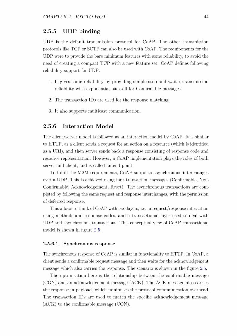
CHAPTER 2. IOT TO WOT 44
2.5.5 UDP binding
UDP is the default transmission protocol for CoAP. The other transmissionprotocols like TCP or SCTP can also be used with CoAP. The requirements for theUDP were to provide the bare minimum features with some reliability, to avoid theneed of creating a compact TCP with a new feature set. CoAP defines followingreliability support for UDP:
1. It gives some reliability by providing simple stop and wait retransmissionreliability with exponential back-off for Confirmable messages.
2. The transaction IDs are used for the response matching
3. It also supports multicast communication.
2.5.6 Interaction Model
The client/server model is followed as an interaction model by CoAP. It is similarto HTTP, as a client sends a request for an action on a resource (which is identifiedas a URI), and then server sends back a response consisting of response code andresource representation. However, a CoAP implementation plays the roles of bothserver and client, and is called an end-point.
To fulfill the M2M requirements, CoAP supports asynchronous interchangesover a UDP. This is achieved using four transaction messages (Confirmable, Non-Confirmable, Acknowledgement, Reset). The asynchronous transactions are com-pleted by following the same request and response interchanges, with the permissionof deferred response.
This allows to think of CoAP with two layers, i.e., a request/response interactionusing methods and response codes, and a transactional layer used to deal withUDP and asynchronous transactions. This conceptual view of CoAP transactionalmodel is shown in figure 2.5.
2.5.6.1 Synchronous response
The synchronous response of CoAP is similar in functionality to HTTP. In CoAP, aclient sends a confirmable request message and then waits for the acknowledgementmessage which also carries the response. The scenario is shown in the figure 2.6.
The optimisation here is the relationship between the confirmable message(CON) and an acknowledgement message (ACK). The ACK message also carriesthe response in payload, which minimises the protocol communication overhead.The transaction IDs are used to match the specific acknowledgement message(ACK) to the confirmable message (CON).
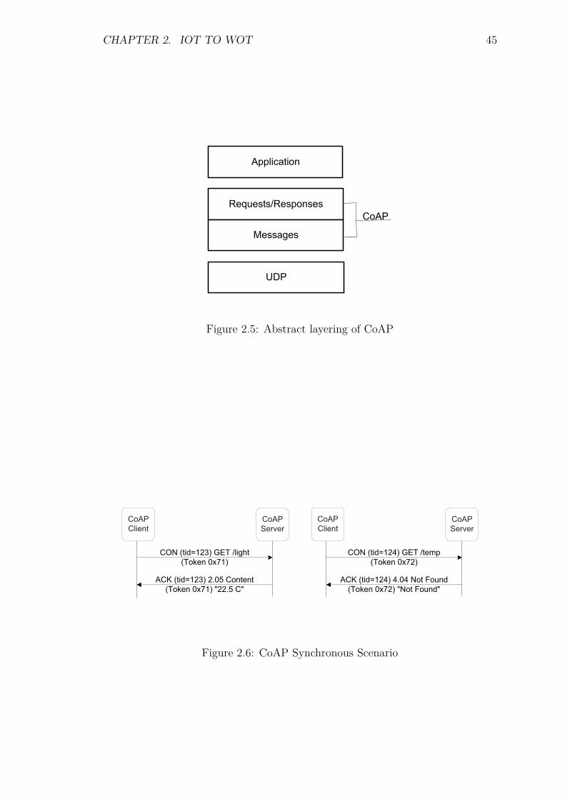
CHAPTER 2. IOT TO WOT 45
�����������
�� � � ���
� ��
���
����
Figure 2.5: Abstract layering of CoAP
���������
���������
� � �������� ��� ����������� �� ��
��! �������� �"�# ����������� �� �� $��"# �$
���������
���������
� � ������%� ��� ��&'������ �� ��
��! ������%� %"�% �� (�)�������� �� �� $�� (�)��$
Figure 2.6: CoAP Synchronous Scenario
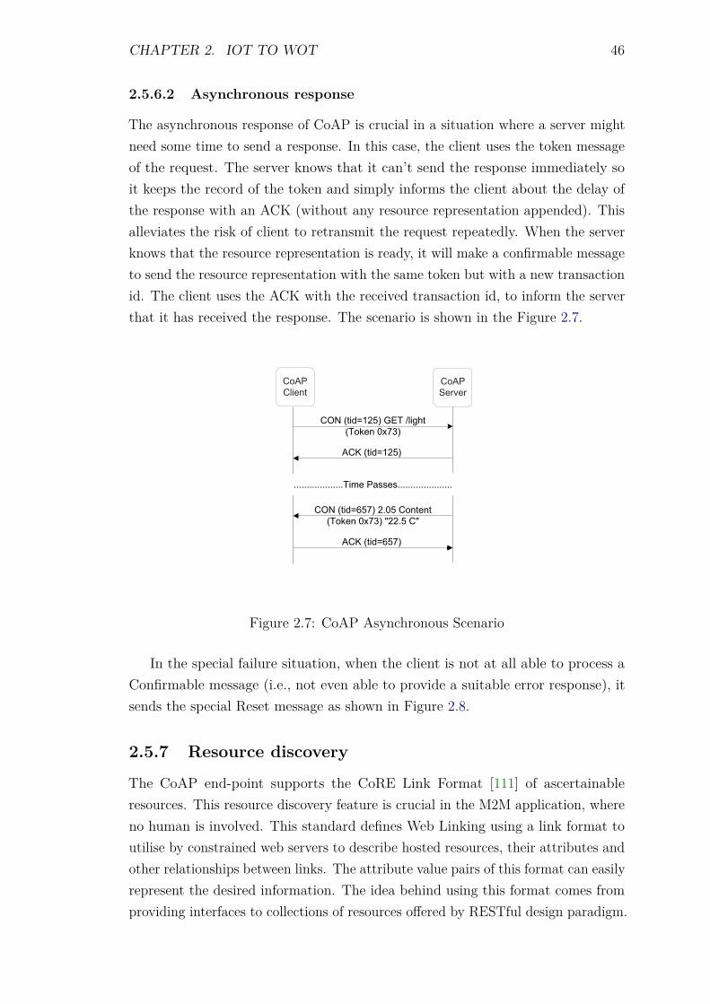
CHAPTER 2. IOT TO WOT 46
2.5.6.2 Asynchronous response
The asynchronous response of CoAP is crucial in a situation where a server mightneed some time to send a response. In this case, the client uses the token messageof the request. The server knows that it can’t send the response immediately soit keeps the record of the token and simply informs the client about the delay ofthe response with an ACK (without any resource representation appended). Thisalleviates the risk of client to retransmit the request repeatedly. When the serverknows that the resource representation is ready, it will make a confirmable messageto send the resource representation with the same token but with a new transactionid. The client uses the ACK with the received transaction id, to inform the serverthat it has received the response. The scenario is shown in the Figure 2.7.
���������
���������
� � �������� ��� ����������� �� !�
��" ��������
� � ����#� � �$�� ����������� �� !� %��$� �%
��" ����#� �
$$$$$$$$$$$$$$$$$$$��&� �'((�($$$$$$$$$$$$$$$$$$$$$
Figure 2.7: CoAP Asynchronous Scenario
In the special failure situation, when the client is not at all able to process aConfirmable message (i.e., not even able to provide a suitable error response), itsends the special Reset message as shown in Figure 2.8.
2.5.7 Resource discovery
The CoAP end-point supports the CoRE Link Format [111] of ascertainableresources. This resource discovery feature is crucial in the M2M application, whereno human is involved. This standard defines Web Linking using a link format toutilise by constrained web servers to describe hosted resources, their attributes andother relationships between links. The attribute value pairs of this format can easilyrepresent the desired information. The idea behind using this format comes fromproviding interfaces to collections of resources offered by RESTful design paradigm.
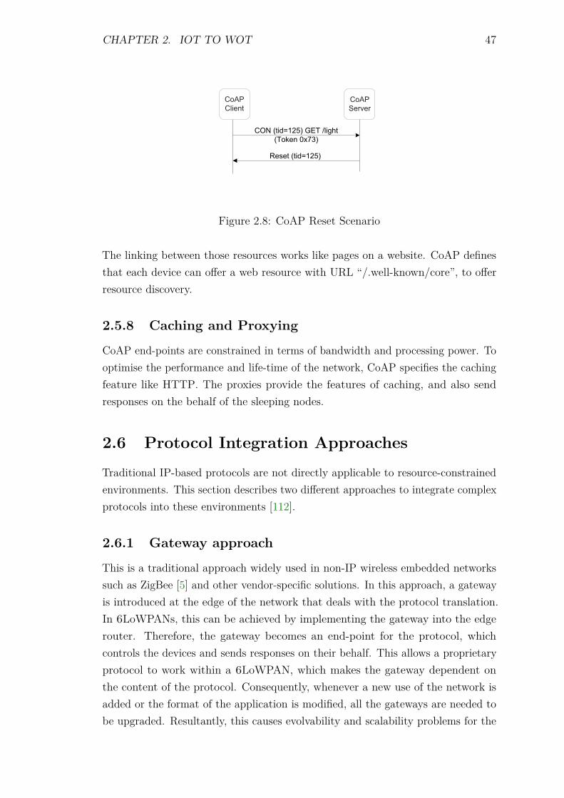
CHAPTER 2. IOT TO WOT 47
���������
���������
� � �������� ��� ����������� �� !�
"�#� ��������
Figure 2.8: CoAP Reset Scenario
The linking between those resources works like pages on a website. CoAP definesthat each device can offer a web resource with URL “/.well-known/core”, to offerresource discovery.
2.5.8 Caching and Proxying
CoAP end-points are constrained in terms of bandwidth and processing power. Tooptimise the performance and life-time of the network, CoAP specifies the cachingfeature like HTTP. The proxies provide the features of caching, and also sendresponses on the behalf of the sleeping nodes.
2.6 Protocol Integration Approaches
Traditional IP-based protocols are not directly applicable to resource-constrainedenvironments. This section describes two different approaches to integrate complexprotocols into these environments [112].
2.6.1 Gateway approach
This is a traditional approach widely used in non-IP wireless embedded networkssuch as ZigBee [5] and other vendor-specific solutions. In this approach, a gatewayis introduced at the edge of the network that deals with the protocol translation.In 6LoWPANs, this can be achieved by implementing the gateway into the edgerouter. Therefore, the gateway becomes an end-point for the protocol, whichcontrols the devices and sends responses on their behalf. This allows a proprietaryprotocol to work within a 6LoWPAN, which makes the gateway dependent onthe content of the protocol. Consequently, whenever a new use of the network isadded or the format of the application is modified, all the gateways are needed tobe upgraded. Resultantly, this causes evolvability and scalability problems for the
CHAPTER 2. IOT TO WOT 48
network and translation increases the delay as each message needs to be translatedtwice.
2.6.2 Compression approach
This approach leads to the compression of existing protocols, so that those canbe made suitable for use over 6LoWPANs. The integration can follow eitherend-to-end or proxy approaches. In end-to-end approach, both application end-points should support the compressed format. Whereas an intermediate proxy canseamlessly translate the messages to, and from constrained end-points in proxybased approach.
Both HTTP and TCP are infeasible to be used directly in a 6LoWPAN. Inliterature, various efforts have used HTTP and TCP, by optimizing existingstandards. Some efforts [29, 30] have used an optimised TCP’s version. Anothereffort [59] has used HTTP’s simple form to provide RESTful web services. TheNanoWS [112] (Nano Web Services) has also tried to transmit binary XML transferusing UDP over 6LoWPANs. Furthermore, the SENSEI project [102] is researchingto find more efficient ways of using web services inside wireless embedded sensornetworks. Another example is CoAP protocol (Section 2.5) that offers a compactversion of the RESTful web services, while offering interoperability to HTTP byseamless translation.
Several standardisation efforts are going underway for the compression of XML.The W3C is working on a standard which will perform compact binary encoding ofXML and is called Efficient XML Interchange (EXI) [109] format. A standard WAPBinary XML (WBXML) [83] format was developed for mobile phone browsers.Another draft proposal called Binary XML (BXML) [41] from the Open GeospatialConsortium (OGC) aims to compress the large set of geo-spatial data. EXIis more suitable technology for 6LoWPANs, as it gives compact representationwithout-of-band schema knowledge.
2.7 Technologies for Experiments
The selection of the technology for experiments is the key to create useful experi-ments and analysis. This section discusses the features of the selected technologiesto emphasise the reasons for their consideration.
2.7.1 Operating System: CONTIKI
This research project employs the CONTIKI [31] operating system for the devices.CONTIKI is an open source, highly portable, multi-tasking operating system

CHAPTER 2. IOT TO WOT 49
for memory-efficient networked embedded systems and wireless sensor networks.It is designed for the micro-controllers with limited memory. There are manyalternatives [35] including the widely known TinyOS. The main reasons to chooseCONTIKI was its high portability, better feature set and an IP stack with RPL [133].It works with both IPv4 and IPv6. Following is the list of CONTIKI’s features:
• Advance IP networking with uIPv6/6LoWPAN protocol stack that supportsRPL.
• Hybrid threading model with protothreads.
• Power profiling mechanism to keep track of energy consumption of each node.
• Text-based shell interface for sensor network interaction and sensing.
• Dynamic loading of the modules.
• Extensive simulation support with COOJA and MSPsim.
2.7.2 Simulator: COOJA
A simulator plays a pivotal role in the code development and testing of anytechnique in constrained networks. The testing and verification of certain algorithmis difficult and tedious without a simulator. Simulators can perform the simulationat application, operating system or hardware levels. The time and overheadincreases, when a node simulates at a hardware level because of the implementationof device drivers. On the other hand, the more high-level simulation does notmodel the node’s hardware; consequently, it restricts the development to the highlevel algorithms only.
COOJA [99] is a novel simulator to be used with CONTIKI OS that enablesthe cross-level simulation (simultaneous simulation at many levels of the system).It is developed in Java but allows to run node software written in C, by using JNI(Java Native Interface). The list of COOJA features are:
• It allows simultaneous simulation at different levels (application, OS, machinecode levels) that makes it distinctive among other simulators [60]. This wayit combines low-level simulation of sensor node hardware and simulation ofhigh-level behaviour in a single simulation [120].
• It works with the Contiki OS (compatible with the choice of OS made inprevious section).
• It can simulate heterogeneous types of nodes in the same network.
CHAPTER 2. IOT TO WOT 50
• It is easily extensible as new plug-ins and radio mediums can comfortably bechanged or replaced.
• It gives a lot of details of the node’s hardware.
The rich features of COOJA; especially its support for hardware-level simu-lations and having heterogeneous nodes in the same network, native CONTIKIsupport and its extensibility were the key reasons to employ it as a 6LoWPANsimulator for this research.
2.8 Summary
This chapter has covered the detail of technologies, which enable the WoT. Thediscussion started with 6LoWPAN architecture and issues related to its integrationwith the Internet. Furthermore, RPL is covered with some detail of its topologycreation and existing application protocol paradigms are discussed in the contextof 6LoWPANs. The emphasis is given to web service paradigm by explaining bothREST and SOAP based web services. This chapter has argued that existing webservices are a poor match for 6LoWPANs, because of there large messages and heavydependence on traditional IP-based protocols. However, compact CoAP basedRESTful web services can be leveraged by these resource-constrained networks.Subsequently, some approaches are explained to integrate existing protocols in the6LoWPANs. In the end, the chapter described the chosen experimental tools.
The next chapter focuses on SD details with the discussion of existing solutionsin literature and analyse them from the perspective of 6LoWPANs.
Chapter 3
Service Discovery (SD) inLiterature
3.1 Introduction
The IoT environment is begin to form with the advent of new technologies such as6LoWPAN. Heterogeneous devices ranging from tiny sensors to powerful devicescan now become an active part of the Internet. These devices provide a variety ofinformation and services. The management and dynamic discovery of these servicesare the tasks of a SDP. Moreover, the demand of efficient and reliable discoveryof network wide services complicate the problem. For example, a user needs toknow the service’s location and communication protocol before he can access it,any time and anywhere. This chapter covers the details of different aspects relatedto SD, including its objectives, existing solutions in literature, design challengesand new perspectives. In addition, some comparative analysis of existing solutionsis presented from the perspective of 6LoWPANs.
3.2 SD Objectives
Services encapsulate the functionalities offered by devices. These provide theabstraction from underlying heterogeneous hardware or implementation details. Inaddition, services can be orchestrated to create new higher-level functionality, andthey can be deployed and executed in remote locations, in-situ on an embeddeddevice if necessary [126]. The function of a SDP is to find the software entitiesor agents that can provide access to required services. An efficient SDP ensuresavailability of optimal services to users and application [3]. The objectives of SDare:
• Dynamic Discovery: The target of SD is to dynamically find a service
51
CHAPTER 3. SERVICE DISCOVERY (SD) IN LITERATURE 52
provider according to the request properties. To fulfil this goal, a SDPneeds a language to describe services, a way to store the service informationsomewhere, and a protocol to search for services.
• Self-configuration: SD has to function without human intervention, i.e. withno administration. This demands the capability of dynamic adaptation ofchanges in topology and service descriptions, while enabling a user withreliable and latest information regarding available services.
3.3 SD Entities
The process of SD is mapping the service description to service location. Thearchitecture of SDPs identifies the building blocks and the links between theparticipating components (entities) [79]. At least following two entities participatein the SD process.
Client (User or User Agent (UA)): The entity, which is interested in search-ing and using a service usually hosts certain applications, which access specificservices. The service request is initiated by this entity.
Server (Service Provider or Service Agent (SA)) : The entity, which hostsand offers services.
Protocols may use service repositories, to facilitate the service mapping proced-ure. Following participating entity is common within SDPs.
Directory (Server, Service Broker or Directory Agent (DA)): Thedirectory node improves the performance of a SDP by acting as a broker orregistry for the discovery process.
3.4 SD Classifications
There is a plethora of SDPs proposed in the literature [2, 79, 87, 88, 129]. Existingprotocols are primarily focused on some specific environments (Ad-Hoc, Mobile Ad-hoc Network (MANET), etc ) mostly other than constrained networks. However, thedescription highlights the interesting features and approaches used for providing SD.This section classifies the protocols according to their architecture, and summarisesthe design details.
CHAPTER 3. SERVICE DISCOVERY (SD) IN LITERATURE 53
3.5 Centralised architectures
A Centralised approach introduces only one centralised directory, which keeps theservice information of the network. Clients generally use to discover the directoryusing broadcast or multicast. However, unicast is used by the clients to advertisetheir services. In a SD scenario, client first contacts a central directory to obtainthe matching service, and then contacts the specific node to invoke it.
This approach is more optimal in the service search context, but it creates asingle point of failure. Centralised architectures depend upon the availability ofa central directory that has a tendency of becoming a bottleneck, as all statusmaintenance traffic flows towards a single point. The scope of SD is also limitedto the devices in the local domain. However, the boundaries of the domain canbe defined administratively to IP subnet or to range of a wireless network. Thissection covers the details of different SDPs based on a central directory.
3.5.1 SLP (Service Location Protocol)
SLP [47] is an IETF standard, and provides a scalable and flexible framework forSD through an IP network.
Entities and protocol: There are three major software entities in the SLP frame-work: UA, SA, and DA. The SA advertises the attributes of hosted services.The service registration with the DA has a lifetime and service needs to reregister after time-out. The SA also replies to the request for services usingunicast. The UA initiates a service request on behalf of client application andreceives a service URL from the DA or SA. SLP can work with or withouta DA. In the absence of a DA, the UA’s service requests is spread in thewhole network, and any SA offering the service would send a reply back.SLP without a DA works well for small networks. In case with a DA, itforms a centralised architecture by placing a DA as tier between UAs andthe SAs, which communicate indirectly through DA. The main function of aDA remains to improve the performance of SLP. The significance of having aDA becomes more apparent in large-scale networks, where the requirementof multicast traffic between UAs and SAs is omitted. The DA works as aregistry which stores all SA advertisements.
Service description and queries: SLP provides service templates [46], whichis an attribute set of searchable service types. The templates include aspecification of attribute: types, default and allowed values. These templatesare used to keep the information of services differentiating between them and
CHAPTER 3. SERVICE DISCOVERY (SD) IN LITERATURE 54
communicate configuration information to UAs. SLP also offers filters forattributes using operators like AND, OR and substrings.
SLP allows multiple DAs; therefore, is scalable. It is flexible, because servicescan be deployed in small networks without any special configuration. It can workwithout Domain Name System (DNS), Dynamic Host Configuration Protocol(DHCP), or routing. Nevertheless, in order to get registered, the address of thecentral directory needs to be known by every SA. It is not dependent to anyprogramming language. Its centralised architecture is vulnerable to a single pointof failure. There is no service selection and service invocation mechanisms arespecified by SLP. Polling is used by SLP to fetch the information from the networkand eventing is defined by SLP. However, some enhancements [62] are introducedfor SLP to adopt subscribe/notify.
3.5.2 SLP-based adaptations and optimised solutions
SLP is not directly applicable to 6LoWPANs as it needs optimisations with moreconsideration to the message size. As in 6LoWPANs, SLP will have 60-80 bytes atthe application layer. Following is the discussion of some research efforts whichhave used SLP ideas to offer SD solution for constrained networks.
SSLP with proximity: The Simple Service for Location Protocol (SSLP) [63]which supports many features of SLP is a draft proposal in the IETF6LoWPAN work group. SSLP provides a simple and lightweight frame-work for the discovery of network services in 6LoWPANs. It uses TokenisedXML strings to minimise the packet exchange. SSLP can also inter-workwith SLP in external IP networks. This can be achieved by using simpletranslation of SLP to SSLP at edge-routers, which enables the clients to dis-cover and control services inside a 6LoWPAN even from outside the network.A proximity-based discovery solution [18] follows the same framework andintroduced a TA (Translation Agent) to translate the SSLP to SLPv2 com-patible type and vice versa. This protocol employs multiple local registriesand uses multicast for the advertisements and status updates. However, itsdependency on gateway marginalise the benefit of using IP for end-to-endcommunication, and the translation between protocols is complex and incursa large overhead.
nanoSLP: nanoSLP [59] is a miniaturised form of SLP that does not supportDA and multicast. The communication between UAs and SAs is allowedusing uni-cast or multicast. In nanoSLP, the resource values are piggybackedin the response to a SD message to save one round trip time. The format
CHAPTER 3. SERVICE DISCOVERY (SD) IN LITERATURE 55
of the request message is also enhanced by using URL instead of a servicename. Consequently, one request can be addressed to several nodes. Thisis a useful feature for a WSN, where nodes are addressed by a geographicallocation (geocasting). The complex search is achieved using one byte encodedcomparison field, called Flags. The drawback is that as the network grows,the burden of multicast increases considerably. Furthermore, nodes havesleep cycles as well, so the discovery process may return without consideringthe sleeping nodes.
nanoSD: nanoSD [69] borrows some ideas of nanoSLP. It has introduced a map-ping tree structure to enable compression of service identifiers into optimalbinary strings. Resultantly, it reduces the packet overhead and also decreasesthe processing and lookup time. Moreover, this structure generates WSDLstyle service descriptions for the backward compatibility with the web-basedback-end systems. The WSDL style service descriptions enable sensor nodesto communicate with the variety of other devices using web services througha gateway.
3.5.3 JINI (Java Intelligent Network Interface)
JINI [9] is a SDP, which relies on the Java language and can be considered as anextension of the Java environment from a single machine to the whole network. Itconsists of service providers, lookup servers and clients.
Service Registration: A service provider uses multicast to find the lookup serverto store services, and respond to clients who need a service.
Service Description and Discovery: Services are stored in the lookup serversin the form of service objects, which have different attributes. The objecthas Java interface for service invocation with other descriptive attributes.The lookup process copies the object to the client, which is then availablefor other clients by object interface. A service is provided to a user on leasebasis, which requires renewal to prolong the validity. The lease time can bevaried in the case of a busy server.
JINI has a rich service description format and supports subscribe/notify mech-anism, where a subscriber of an object gets notification of the changes. The majordrawback of JINI is that it requires each device to either run a Java virtual machineor to associate itself with a device (proxy) that can execute a JVM on its behalf.It also needs reliable, stream-oriented communication and a multicast facility.Furthermore, JINI makes the assumption about the capabilities of RAM and CPU
CHAPTER 3. SERVICE DISCOVERY (SD) IN LITERATURE 56
power of the devices connected to the network. It also requires the Java VirtualMachine (JVM) and Java Remote Method Invocation (RMI). A service proxy posesan extra challenge, that all the devices should have the common interface, which isnot feasible, as no implementation standard is defined for JINI.
3.5.4 Salutation
Salutation [105] is an architecture for SD, proposed by Salutation Consortium thatis non-proprietary and primarily solves the problem of SD and can be utilised byheterogeneous devices and network technologies. The development of a transport-independent SD solution was the main aim of the designers.
Entities and Protocol: Its architecture consists of three components: Functionalunits, Salutation manager (SM), and transport manager (TM). A functionalunit defines services using a descriptive attribute unit. A service providerlocates a nearby SM and registers itself with it. The SM is a registry ofservice providers and their services, similar to JINI lookup service. Duringthe discovery client contacts local SM to locate a service. The search isthen performed with the coordination among the SMs. The RPC is used forthe communication. The TM is responsible for providing reliable channelindependent of underlying transport, but it can support one network transportat a time. Therefore, if devices are using many different transport protocols,each is handled by a separate TM. The SM not only acts as a service registry,it also discovers services and manages the sessions.
Salutation is independent of employed transport protocol. Salutation-lite isthe lighter version of Salutation for constraint devices and networks. It primarilyfocuses on SD and waives optional functions. The Salutation consortium wasdissolved in 2005 and its specification is no more maintained on the website.Consequently, it can’t cope with the new challenges posed by drastically differenttechnologies including 6LoWPAN.
3.5.5 FRODO (Framework for Robust andResource-aware Discovery)
FRODO [121] SDP targets the home environment with a limited number of devices.It focuses on two main issues of resource-awareness and robustness. It definesits own communication protocol which makes it independent of the underlyingnetwork.
CHAPTER 3. SERVICE DISCOVERY (SD) IN LITERATURE 57
Resource Awareness: FRODO address resource-awareness by specifying threedifferent types of devices which include 300D (powerful devices), 3D (mediumcomplex devices), and 3C (simple devices). The architecture of FRODOconsists of users (who use services), managers (who provide services) andregistries (who store service information). It elects one of the most powerful300D node as a registry. Another node is selected as a backup registry, whichtakes the responsibility of a central directory in the case of failure. Theavailability of a backup registry provides the robustness by making FRODOresilient to single point of failure. Both solicited/unsolicited registrationmechanisms are used in FRODO; it depends on the device’s capabilities. Thestate is maintained by polling the registry in case of a resource constraineddevices like 3D and 3C. On the other hand, the powerful devices like 300Dperiodically poll the registry by themselves.
3.5.6 SLEEPER
Sleeper [15] is a SDP, which uses proxy advertisement and discovery to reduce theworkload from power constrained nodes. It has a special emphasis on limiting thepower consumption of devices. The advertisement structure supports several modesof SD, including conventional service advertisements, meta discovery, taxonomic-based discovery, location-based discovery and federated discovery. Both pull, andpush modes of advertisement are used by the protocol. Service popularity attributei.e. number of times a node is called for a service in a recent time window, is usedas a decision criterion to select the respective mode of advertisement.
Energy efficiency: Sleeper uses an algorithm to select a proxy node with respectto capability criteria. The other service nodes can be in a state of online, offlineand standby. In the online state, a service node advertises its services, servicepopularity and capabilities to the proxy. The node can go to stand by modeuntil it receives the signal for service provisioning. The proxy periodicallybroadcasts the service information and popular advertisement. Sleeper isanalytically compared to Universal Plug and Play (uPnP), Simple ServiceDiscovery Protocol (SSDP), and DEAPspace and the analysis promisescomparable response time with the benefit of power saving [15]. However,the criteria for selection of proxy nodes and design issues of proxy nodes in ageographical network are not addressed by the protocol.
CHAPTER 3. SERVICE DISCOVERY (SD) IN LITERATURE 58
3.5.7 Splendor
Splendor is a SD model which emphasises security and supports privacy. Locationawareness is used to decrease the discovery network infrastructure [138].
Protocol: The initial communication between clients and a directory is doneusing multicast. The protocol assumes that all parties know the multicastaddress in priori. All service information is registered on predefined directorynodes. A client can directly query to a directory node to discover serviceswith unicast requests. The directories cache service information and respondto queries.
Security: Services and clients use certificates to verify and authenticate the dir-ectories. Splendor supports mobility by keeping the soft states of services andwith periodical directory advertisements. It also stores services representedby proxies as a hard state in directories. The directories explicitly queryproxies about status of services. The use of proxies also enables Splendor tooffer security and privacy features.
3.6 Distributed architectures
In this architecture, many directories are maintained in a network which hold theservice information of the nodes in their vicinity. DNS based protocols ensurescalability by using a hierarchical architecture. Cluster-based protocols do notuse the preselected directories. Instead, directories are elected based on suitablecapability, which can be battery power, node coverage, memory, or processing power.Hash-based protocols built peer-to-peer overlay networks and offer distributed hashtables (DHT). The significance of using distributed directory-based architectureincreases, as size of a network becomes larger.
This section covers the detail of various distributed directory based approaches.
3.6.1 Domain Name Server (DNS) based
DNS is employed to translate human readable names to IP addresses. However, itassumes that sets of Internet host names (domain names) and addresses do notchange frequently. Consequently, registration just follows a static process type.New pairs of domain names and addresses are stored at a designated server. Thelookup process starts when a client sends a query to local host. At first, the localhost checks its DNS entries. If it can’t provide the mapping, it passes the query toDNS server one level up in hierarchy. The location information of the next DNS
CHAPTER 3. SERVICE DISCOVERY (SD) IN LITERATURE 59
server is configured for a host. Following is the detail of some of the protocolswhich follow DNS architecture for SD.
GloServ: GlovServ [8] is a global SD architecture to locate local and wide-areaservices. The architecture of GloServ is similar to DNS, which contains rootname servers and authoritative name servers to manage the information ofservices. The DNS like structure is used to provide scalability. Services aredefined in Resource Description Framework (RDF) and queried using theRDF Query Language (RQL). The RDF also enables a service to includecontextual information. The service classification on high level is based ongeneral categories like events, services, people and places.
A SA can register its service to GloServ by specifying the particular point inthe hierarchy. URNs (Uniform Resource Names) are used to reference servicesin GloServ, because services can support different protocols such as HTTP,SIP and others. RDF specifies the mapping of a service to URN and detailsof its properties. A UA which already holds a copy of the updated servicehierarchy, queries directly for a particular service on behalf of a user. Theformats used by this protocol are verbose and require a number of packets tocommunicate a single message in constrained networks such as 6LoWPANs.
Electronic Number Mapping (ENUM) based SD: Thisis an attempt to adopt the DNS based architecture in 6LoWPANs usingENUM-based numbers to provide SD [7]. ENUM assigns E.164 numbers [14](unique identifier) to services to make them globally accessible. The archi-tecture consists of sensor nodes and few master nodes. Each sensor nodeis associated with a master node. The gateway is used to communicatewith the outside network. Sensor nodes are computationally constraineddevices, which depend on master nodes for communication with the gateway.Therefore, master nodes not only forwards the sensor nodes’ requests togateway, but also passes services destined for them. The protocol translatesE.164 numbers to domain name and sends it to DNS server to get matchingName Authority Pointer (NAPTR) [86] records. These records are resolvedinto URIs which are returned to the clients.
The protocol assumes that DNS lookup will always be able to find matchingNAPTR records, and sensors (multi-hop distance away from master node)must know the route towards the master node. However, the use of E.164numbers and NAPTR format reduces the message size and results in lowlatency and bandwidth utilisation.
CHAPTER 3. SERVICE DISCOVERY (SD) IN LITERATURE 60
3.6.2 Clustering based
In this approach, a set of nodes is elected as act like distributed directories. Thesenodes act like hubs for the neighbour nodes, as all SD messages travel among them.This approach restricts the use of multicast and consequently, reduces the networktraffic significantly. To address the issues of both latency and energy conservation,Clustering in the wireless sensor network has proven to be the most efficient [82].
Clustering for Service Discovery (C4SD): Clustering for service discovery(C4SD) protocol [81] selects the cluster nodes and cluster heads based ontheir capabilities. The cluster heads act as directories, and other nodesregister services with the cluster heads in their vicinities. A service requesterjust needs to query the cluster heads to discover services, which reducesthe communication cost. Furthermore, the lightweight clustering algorithmsbuild the distributed directory of service registration based on only thoseneighbours who are one hop away. It reacts rapidly to topological changesand resultantly provides the basis for energy-efficient SD. The protocol alsoconsiders low maintenance overhead while reducing the chances of issuese.g., chain reaction problem.
However, solution still exhibits the potential of facing chain reaction problem.Moreover, re-clustering and re-registration are costly in a network with thelarge number of clusters.
Sailhan: Sailhan [106] is a scalable SDP for large-scale (100s of nodes) MANET.The architecture of Sailhan is structured as a virtual network of distributedand dynamically deployed directories.
In this approach, directories are elected among all the nodes in a network withthe criteria of available resources and context parameters. Each directorykeeps the information regarding available services in neighbour nodes withina fixed number of hops. The WSDL standard is used to define a servicedescription. Directories co-operate with each other by exchanging theirprofiles between them. The shared profile consists of capacity of the node andcondensed list of service information created using bloom filter technique. Aclient sends a query for a service to its local directory. At first, local directorytries to find the service in its cache. In case of failure, it initiates globaldiscovery by forwarding the query to selective directories. The criterion ofthe selection is based on the information provided by shared profiles.
The protocol assumes a MANET with nodes holding the same networkinterface, with IP-level connectivity using the underlying routing protocol.However, it also poses a prerequisite of some gateway nodes which hold
CHAPTER 3. SERVICE DISCOVERY (SD) IN LITERATURE 61
interfaces to several networks, either ad hoc or infrastructure-based. Thisdefines a bridging between hybrid networks (MANETs and infrastructure-based networks), according to the specific networking capabilities of thewireless nodes [22]. This protocol is designed specifically for MANETs;consequently, it doesn’t address the challenges posed by 6LoWPANs.
SANDMAN: SANDMAN [108] is a cluster based SDP designed for MANETsthat concentrates on power saving. It groups the nodes with similar mobilitypatterns into clusters. A Cluster Head (CH) is elected among the nodes tostay awake permanently and responds on behalf of other nodes in the cluster.The other nodes sleep most of the time, and periodically wake up to updateCH about their presence and service status. The protocol also offers the loadbalancing technique to re-elect the CH occasionally.
The evaluation results show that SANDMAN saves energy up to 40% ofservice requests. The rationale is that more energy can be saved by increasingthe size of a cluster, but this also increases the delay. As the cluster sizeincreases, requesting client has to wait more for the sleeping node to wakeup. However, the performance can be improved by adaptive selection of idleand sleep times.
Service Rings: Service Rings [67] is a scalable SDP designed for MANETs. Thenetwork is clustered into rings, which creates a hierarchal ring structure.The nodes that are physically closed and offer similar services are groupedinto rings. Every ring contains a Service Access Point (SAP) and know onlyabout it predecessor and successor rings. SAP in the last ring is called worldring. A node keeps information about all services offered by the ring in itsSAP. The protocol devises algorithm for ring restructuring, splitting andmerging to optimise ring’s structure. Rings use those algorithms to decidedynamically, about their structure, to monitor network traffic efficiently. Achosen SAP periodically initiates a ring check message, which is circulated inthe ring to verify the consistency of the network. In the case of a breakageor a partition, the selected SAP starts a ring repair or integration algorithm.
Service rings protocol has not defined any format for service descriptions.SAP in every ring is used to store service information, and are queried todiscover a service. It also supports the mobility as rings are maintained withperiodic ring check messages. The efficiency of the protocol depends on theeffective selection of the nodes in every ring (with the similar services andefficient links between them), and the appropriate size of a ring (neither toosmall nor too big).
CHAPTER 3. SERVICE DISCOVERY (SD) IN LITERATURE 62
LANES: LANES (A Lightweight Overlay for Service Discovery in Mobile Ad HocNetworks) [66] is a SDP which is based on Content Addressable Network(CAN) [103] structure. It creates a two-dimensional overlay structure ofthe network by grouping nodes into lanes. One dimension is responsible fordisseminating service advertisements, whereas other dimension distributesservice requests. Every node in the lane pro-actively broadcasts its servicesto other nodes, and keeps the cache of services in the lane. However, thelanes are loosely coupled with each other and reactively forward the queriesto other lanes using any-cast.
Service descriptions are distributed to
√Nnodes
where N is the total number of nodes in a network. The protocol is independ-ent of any service description format. A periodic ping message is used tocheck and maintain the lanes. Furthermore, protocol defines the algorithmsto split and merge the lanes to achieve their optimal size.
Virtual Service Overlay (VSO): Virtual Service Overlay (VSO) [94] approachcreates a virtual overlay of a network based on service types. It createsa service-centric overlay to provide better energy conservation, instead ofnetwork centric model which focuses on the physical location of nodes. Nodesuse Service Capability Messages (SCAP) to get the knowledge about networkwide available services. Every node broadcasts the SCAP message andmaintains a table of other peer nodes offering the similar services. The peernodes multicast “vDA Interest” messages among them to elect a virtual DA.This elected DA matches, compares and aggregates services provided by thesimilar peer nodes. In addition, it also searches for the closed match servicesoffered by a resource-rich node in the neighbourhood. The virtual DA isre-elected periodically for load balancing.
VSO emphasises on providing better service quality by aggregating services.It also claims to improve overall energy conservation and congestion control.
3.6.3 Hash-based P2P
The protocols categorised in this class rely on peer-to-peer (P2P) overlay networksthat are constructed using Distributed Hash Tables (DHT). The examples includeChord, Pastry, Content Addressable Networks (CAN), Tapestry. DHT is used tostore a key-value pair on designated nodes. The hash function is applied to the
CHAPTER 3. SERVICE DISCOVERY (SD) IN LITERATURE 63
message and is passed to the responsible nodes in the fixed number of hops. Everynode keeps a routing table with network addresses of neighbour nodes.
The main advantage of using DHT based protocols is their scalable and efficientlookup mechanism. The lookup is performed within O(log(N)) hops, where ‘N’is number of nodes in the overlay network [79]. However, the downside is that itgenerates considerable network traffic and a maintenance overhead, which makes itless suitable for the WSNs [80]. The search is based on a unique identifier, whichis only useful for searching services with a unique name. Conversely, effectiveattribute-based searches are still not supported by DHTs.
Following is the detail of a Tapestry which is based on hash-based approach.
Tapestry: Tapestry [137] is a peer-to-peer (P2P) decentralised architecture, whichprovides a fault-tolerant, scalable and robust wide-area infrastructure tolocate the required services. It efficiently constructs an overlay network usingdistributed algorithms. It assigns Globally Unique identifier (GUID) to anobject’s unique identifier. The object ID with a “salt” value is hashed toidentify appropriate roots. Tapestry dynamically maps each GUID to aunique live node called the object’s root. Tapestry assigns multiple rootsto each object. The message to a node is routed to its root. If in the way,any node found with the location mapping to the destination, then it isimmediately passed to the node that contains the object. In other cases, themessage keeps on traversing the hierarchy towards the root. The root to anode always got the required mapping.
3.7 Directory-less architectures
The protocols with directory-less architecture use multicast or broadcast to dis-cover a service. These protocols incur the overhead when services are discovered.Therefore, this kind of solutions can be efficient in a small-scale network. How-ever, these solutions are not feasible for a medium or large-scale network, as thecontrol overhead can overwhelm the network. Furthermore, node’s sleep cyclein constrained networks such as 6LoWPANs can result in a discovery based onincomplete information. Some popular protocols of this domain are described inthis section.
Bonjour: Bonjour [118] is Apple’s version of Zeroconf [40] networking, which isbased on a combination of the multicast domain name system (mDNS) [21]and DNS-SD [71]. It targets service and device discovery among computersand other networked devices. Bonjour provides zero-configuration by assign-ing IP addresses to the devices, without the aid of DHCP server. A new
CHAPTER 3. SERVICE DISCOVERY (SD) IN LITERATURE 64
service provider in a network uses multicast to advertise its presence to otherdevices. Clients receiving the advertisement cache service records for a spe-cified time. In discovery scenario, a client multicasts a query with the detailsof domain name, service type and preferred communication protocol. Serviceproviders with the matching DNS entries respond with service records.
Bonjour generates a significant amount of traffic by using multicast extensively.This issue is addressed by the protocol by using exponential back-off, whichincreases the time interval between queries and announcements. The relianceof protocol on multicast results in heavy traffic, more energy consumption andcongestion. Therefore, bonjour is only suitable for very small scale networksand high bandwidth usage makes it a poor match for resource constrainednetworks.
uBonjour (Compressed Bonjour): uBonjour [64] is bonjour’s compact form,based on mDNS and DNS-SD. This protocol works like bonjour, but com-bines different messages to decrease the control overhead. Even thoughmDNS/DNS-SD message sizes were recently optimised for 6LoWPANs [65],uBonjour still relies on the availability of IP multicast and entails more com-munication overhead. The compression requires more changes and processingat the gateway to decode the information.
Universal Plug and Play (uPnP): uPnP1 was proposed by Microsoft for deviceand SD in small office and home environments. The main features of uPnPare its zero-configuration and automatic discovery of heterogeneous devices.It is independent of any programming language or operating system. UPnPuses protocols, including HTTP, TCP/IP and SOAP. Zeroconf feature en-ables it to assign IP addresses automatically to devices, if no DHCP serveris available. Its architecture consists of devices, services and control points.Every device needs to provide an XML device description document, whichcontains the list of services and properties of the device. A service storesits state information in state table, and supports a control server to updateits state table. The subscribers to a service are also managed by its eventserver. Control points act as directories and are optional. UPnP’s discoveryis based on Simple Service Discovery Protocol (SSDP), which uses HTTPand SOAP over TCP multicast (query request) and UDP unicast (using aservice by specifying URL).
UPnP generally operates better over reliable networks, so it is unsuitablefor networks with lossy links and other constraints. It is based on HTTP,
1http://upnp.org
CHAPTER 3. SERVICE DISCOVERY (SD) IN LITERATURE 65
and SOAP protocols, which are heavy and verbose for a resource constrainednetworks. Moreover, it does not support attribute-based querying for services.The extensive use of multicast makes uPnP non-scalable and also exhauststhe energy of the devices in a network.
DEAPspace: DEAPspace is a peer-to-peer SDP for single-hop short-range wire-less systems [95]. The DEAPspace uses the proactive SD framework. Devicesperiodically broadcast their services and keep information of all servicesavailable in their one hop proximity. Each device also specifies the timeperiod, during which the service is valid. After expiration, the device shouldrenew its service description, or it is marked unavailable for its neighbours.
A performance evaluation [74] shows that time for discovery is better in thecase of DEAPspace when compared to other broadcast-based push models.However, the periodic broadcasts consume much of the network bandwidth,which makes DEAPspace unsuitable for constrained devices and networks.
Group-based Service Discovery (GSD): GSD [16] is based on peer-to-peercaching of service advertisements and forwarding of service requests. Servicedescriptions are defined in DARPA Agent Markup Language (DAML+OIL).It uses the semantic information of DAML to create a service hierarchy tocreate service groups. The protocol does not broadcast service requests, butinstead it exploits semantic information to selectively forward to the nodeswith similar services. The more flexible service matching mechanism is alsoprovided by the protocol using DAML format of service information.
Each node periodically advertises its list of services to all nodes in its vicinity(particular number of hops) and caches their service information. The servicegroup information is also disseminated with the advertisement. On receivinga service request, the node multicasts the request to its other group members.The parameters like advertisement expiration period and range of hops can bespecified according to the network. Semantic service definitions have meritsof grouping of nodes and better service matching, but these also increase theenergy consumption and require large packet size.
Konark: Konark [50] is peer-to-peer SD and delivery architecture for multi-hopad hoc networks. It is based on lightweight HTTP servers, and uses SOAPto handle service delivery. It also defines WSDL based service descriptionlanguage. Konark supports both push and pull modes of SD. The proactiveor reactive service advertisements are used on the need basis. A serviceadvertisement specifies its time-to-live and enables its caching on each node.
CHAPTER 3. SERVICE DISCOVERY (SD) IN LITERATURE 66
In Konark, each device runs a lightweight HTTP server and uses multicastto advertise services. Every node maintains a service registry to store serviceinformation. The registry is based on a tree structure with a number oflevels to classify services. A service request can query for a generic or specificservice in each category, so it can carry simple keywords or more preciseservice description. The multicast is used to send forth service requests toa fixed group; corresponding nodes with the matching service will respondback using unicast.
Service advertisements of Konark allow semantic matching and are lighterthan WSDL, but still increases the energy consumption. The use of multicastfor service requests is also costly for restricted networks where bandwidth islimited and links are unreliable. Konark doesn’t address the issues of energyconsumption and delay, which have significant importance in constrainednetworks.
Bluetooth SDP: Bluetooth SDP [12] targets the bluetooth devices with limitedcomplexity. Therefore, it is optimised and partly addresses SD. It providesa simple API for enumerating the devices in one hop range and browsingthrough available services. It offers no feature of service advertisement,registration, or invocation. Services are described in attribute-value pairs,which are searched by service type without a priori knowledge of serviceattributes. The features like selection, access and usage of services are alsonot defined by the bluetooth SDP. Moreover, services can become unavailablewithout any notification.
3.8 Cross-layer design
The cross-layer SDPs extend the routing mechanism to find the routes and discoverservices offered by that node. It is obvious that by piggybacking the serviceinformation onto routing messages decreases the number of messages needed forSD and routing. Resultantly, the less traffic increases the available bandwidth, andenergy is also saved.
The cross-layer SD was first proposed by R.Koodli [68]. A similar approachbased on Ad-hoc On-demand Distance Vector (AODV) [38] extended the function-ality of the routing protocol. SD-AODV and SD-DSR [48] extended AODV andDynamic Source Routing (DSR) to support SD. These approaches outperform theapplication-layer SDP based on SLP. A proactive routing protocol Destination-Sequenced Distance Vector (DSDV) was extended in the similar way [34]. Thecomparison has shown that reactive SD-DSR performed best in terms of messaging
CHAPTER 3. SERVICE DISCOVERY (SD) IN LITERATURE 67
overhead, when compared to SD-DSDV and SLP. Some extensions of routingprotocols [127] and [51] have also considered the issue of energy consumption.
SPIZ (Service advertisement and discovery Protocol with Independent Zones) [96],a hybrid integrated protocol (based on multiple criteria such as mobility and ser-vice popularity) performed better than SD-AODV solution. The extension ofOn-demand multicast routing protocol (ODMRP) that uses multicast and onlyresend advertisements if service changes [75]. An approach [49] used High EfficiencyService Discovery (HESED) multicast routing protocol for both service requestsand responses. LIFT (Limited Flooding of requests within a clusTer) SDP [134]divides a network into clusters with some High Capability Devices (HCD) as acluster leader. The SD-AODV is extended with the cluster-based SD approach,which further decreases the energy consumption. Another approach Multi-pathCross-layer Service Discovery (MCSD) [110], finds multiple routes to service agentsand provides better service availability and network layer performance.
In summary, the cross-layer design and optimisations can be used to improvethe performance of a protocol. The main idea is to control and exchange ofinformation over different layers in the architecture for efficiency. However, thereare cons of using cross layered architecture in a WSN. Architecture violationsmake the protocol hard to maintain by increasing the complexity of later updates.Furthermore, the luxury of designing protocols at different layers independently isalso violated by the cross-layer design.
3.9 Discussion from 6LoWPAN’s perspective
WSNs are resource-constrained environments, which consist of highly resourceand power limited nodes with very low data rate communication. The nodescommunicate over IEEE 802.15.4 radio channel and have few kilobytes of RAM andabout 100 kilobytes of ROM. The mostly battery operated nodes are not rechargedquite often, thus need to run for longer periods. This domain poses more difficultrequirements for SD than others. The limited bandwidth and power do not allowheavy traffic and necessitated acknowledgements for guaranteed packet delivery ina lossy environment. The limit to typical packet size is 127 bytes, which is furtherreduced at the application layer to only 60-80 bytes (Section 2.2.2).
These limitations along with the node’s memory and processing capabilitiesrestrict the use of a resource and computational hungry protocols. The nodes alsohave sleep cycles to conserve power, which needs to be considered by a SDP. Thesereasons do not allow most popular protocols like UPnP and SLP to work directlyfor 6LoWPANs. To make those functional, their features should be minimised, andsome compression mechanism should be used for their verbose formats. The trade-
CHAPTER 3. SERVICE DISCOVERY (SD) IN LITERATURE 68
off between the computational complexity and compression ratio should be managedfor applicability. Some extreme approaches focuses just on performance gain forthese constrained networks include the cross-layer optimisations (Section 3.8) andmerging of SD and data collection functionality like TinyDB system [77]. Anothersuitable approach is to use attribute based naming scheme [87], which also workon lower layer in the protocol stack to improve the performance of the network.In addition, other functions like data aggregation and in-network processing canbe used, which make use of intermediate nodes to do the aggregation of data tosave the power and bandwidth of the network. These approaches only benefit thespecified single application and also lose the potential of using layered architecturefrom extensibility perspective.
Traditionally, there are three types of SDPs: Centralised, Directory-less anddistributed directory based approaches. The comparison of different architecturesis given in Table 3.1.
The centralised directory and cluster based architectures (Section 3.5 and 3.6.2)are mostly suited for a network with the element of heterogeneity. These archi-tectures exploit the power of more resource-rich devices by making them servers,to assist the other nodes by sharing computational load. In some approaches, thegateway registers the nodes in a network using special optimised protocol [19]. Itacts on behalf of registered nodes and can support multiple external SDP architec-tures. The distributed hash-baed P2P (peer-to-peer) approaches (Section 3.6.3)can also be employed in WSNs. This type of approach treats all nodes equally, butuses multicasts and broadcasts, which can overwhelm the network by generatingheavy traffic.
Directory-less protocols, as the name suggests, work without any specific nodesto act as registries and make use of flooding mechanisms to discover a service. Inthis approach devices cache the service information of the neighbours to enhancethe SD process. UPnP, Bluetooth SDP, DeapSpace and Konark are popular SDPsof this domain. However, the extensive use of multicast or broadcast make thiskind of SDPs unsuitable for the resource constrained 6LoWPANs.
Distributed architectures consist of multiple registries, which act as a serviceinformation container of their vicinity. These registries collaborate between them bypassing the request to each other for discovery. CS4D, Service rings and Lanes arethe examples of this technique. Sailhan has optimised the forwarding by periodicinformation sharing among registries. Other approaches, including SANDMANconserve energy of the nodes by keeping the nodes sleep while keeping their clusterheads awake to respond on behalf of them. VSO approach has defined the criteriaof creating clusters based on the type of services, rather than node’s locality. Thismethod can be useful in scenario where similar kinds of services are available in
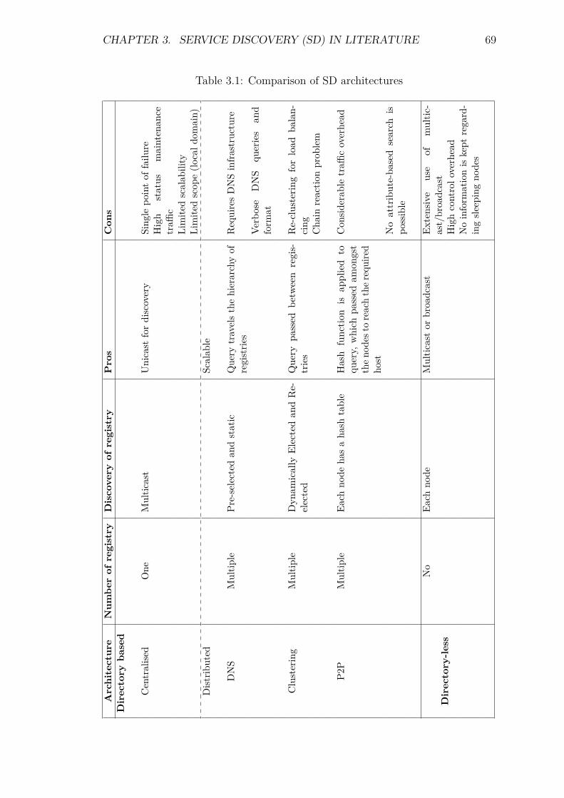
CHAPTER 3. SERVICE DISCOVERY (SD) IN LITERATURE 69
Table 3.1: Comparison of SD architectures
Architecture
Num
berof
registry
Discovery
ofregistry
Pros
Con
sDirectory
based
Centralise
dOne
Multic
ast
Unicast
fordiscovery
Sing
lepo
intof
failu
reHigh
status
maintenan
cetraffi
cLimite
dscalab
ility
Limite
dscop
e(lo
cald
omain)
Dist
ributed
Scalab
le
DNS
Multip
lePr
e-selected
andstatic
Que
rytravelsthehierarchyof
registrie
sRequiresDNSinfrastructure
Verbose
DNS
queries
and
form
at
Clustering
Multip
leDyn
amically
Elected
andRe-
elected
Query
passed
betw
een
regis-
tries
Re-clusterin
gforload
balan-
cing
Cha
inreactio
nprob
lem
P2P
Multip
leEa
chno
deha
saha
shtable
Hash
functio
nis
applied
toqu
ery,
which
passed
amon
gst
then
odes
toreachther
equired
host
Con
siderab
letraffi
coverhead
Noattribute-ba
sed
search
ispo
ssible
Directory-less
No
Each
node
Multic
astor
broadcast
Extensiv
euse
ofmultic
-ast/broadcast
Highcontrolo
verhead
Noinform
ationis
kept
regard-
ingsle
epingno
des
CHAPTER 3. SERVICE DISCOVERY (SD) IN LITERATURE 70
different clusters, and most of these services are queried together. Distributed SDPssave energy in the case of service status maintenance, but overhead of creatingclusters can overwhelm the network. Moreover, the chain reaction problem furtherargues against the clustering for a SDP for 6LoWPANs.
The directory based infrastructure can be more feasible for 6LoWPANs. Theadaptation layer needs an edge router to connect a PAN to the Internet. Edgerouter can be used as a main directory for 6LoWPANs. The well-known industry-standard IP based SDPs include SLP, UPnP, JINI and Salutation. Table 3.2 showsthe comparison of most popular SDPs with respect to 6LoWPAN SD requirements.All these protocols are not directly applicable to constrained 6LoWPANs andmost of them are based on TCP/IP, which creates further problems in theiradaptation [89]. JINI lacks the versatility as it is language-dependent and needsservice information in the form of Java objects. In the same way, NanoSD assumesthat each participating node has enough memory to keep the cache of serviceinformation. However, the extensive use of multicast and broadcast make this kindof SDPs unsuitable for resource constrained 6LoWPANs.
There are some efforts, which have tried to adapt the SLP for 6LoWPANs.NanoSLP, a miniaturised version of SLP, is an attempt to use SLP with the reducedfeatures and only supports the directory-less architecture. Another attempt wasthe SSLP [63], which proposes a compact version of SLP for 6LoWPANs. Aproximity-based approach [18] which uses DPAs (Directory Proxy Agents)as localregistries has employed SSLP inside a 6LoWPAN and provided the interoperabilitywith SLP by using a Translation agent (TA). However, this solution involvescomplexity and delay of translation, each time message is translated to or fromSLP. Furthermore, the casual sharing of resources between distributed directoriesincreases the traffic burden. uBonjour [64] is bonjour’s compact version, based onmDNS and DNS-SD. Even though mDNS/DNS-SD message sizes were recentlyoptimised for 6LoWPANs [65], uBonjour still relies on the availability of IPmulticast and entails more communication overhead for service registration andstatus maintenance. ENUM-based approach [7] also requires some master nodes.This technique introduces compression for 6LoWPANs, and has assumptions, whichdepend on the availability of the required information and database entries. ATCP/IP based web portal’s mechanism [104] is employed using regional locals(master nodes) for the local SD and data servers are used in a network, whichprovides a complex mechanism which increases cost burden. RSDPP (Real-WorldService Discovery and Provisioning Process) [44] is an industry focused SOA(Service Oriented Architecture) based middle-ware solution that uses SOAP-basedor RESTful web services. DiscoWoT [84] provides RESTful web services usingHTTP based SD with existing or injected strategies. However, this scheme has
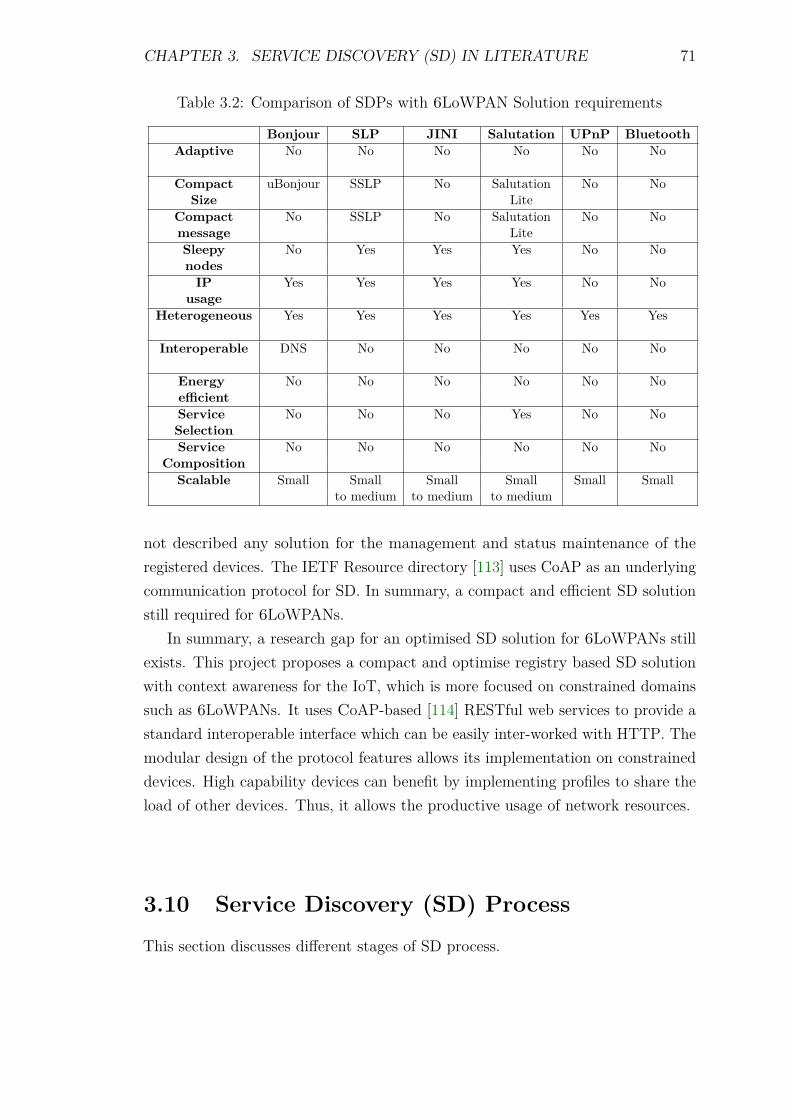
CHAPTER 3. SERVICE DISCOVERY (SD) IN LITERATURE 71
Table 3.2: Comparison of SDPs with 6LoWPAN Solution requirements
Bonjour SLP JINI Salutation UPnP BluetoothAdaptive No No No No No No
Compact uBonjour SSLP No Salutation No NoSize Lite
Compact No SSLP No Salutation No Nomessage LiteSleepy No Yes Yes Yes No NonodesIP Yes Yes Yes Yes No No
usageHeterogeneous Yes Yes Yes Yes Yes Yes
Interoperable DNS No No No No No
Energy No No No No No NoefficientService No No No Yes No NoSelectionService No No No No No No
CompositionScalable Small Small Small Small Small Small
to medium to medium to medium
not described any solution for the management and status maintenance of theregistered devices. The IETF Resource directory [113] uses CoAP as an underlyingcommunication protocol for SD. In summary, a compact and efficient SD solutionstill required for 6LoWPANs.
In summary, a research gap for an optimised SD solution for 6LoWPANs stillexists. This project proposes a compact and optimise registry based SD solutionwith context awareness for the IoT, which is more focused on constrained domainssuch as 6LoWPANs. It uses CoAP-based [114] RESTful web services to provide astandard interoperable interface which can be easily inter-worked with HTTP. Themodular design of the protocol features allows its implementation on constraineddevices. High capability devices can benefit by implementing profiles to share theload of other devices. Thus, it allows the productive usage of network resources.
3.10 Service Discovery (SD) Process
This section discusses different stages of SD process.
CHAPTER 3. SERVICE DISCOVERY (SD) IN LITERATURE 72
3.10.1 Service description
Every SDP needs a way to describe services. Therefore, a service descriptionmechanism is essential for any SDP to function. Different protocols use unlikeformats of service description to enable users to search for a particular service bysetting fields and values according to the format. A service description generallycontains the identity and type of a service with optional attributes.
Generally, SDPs use classes to classify services into service types. Each serviceclass (e.g., print class for print-related services) contains a list of attributes, whichare assigned with values to identify the instance of the class. A service descriptionis usually stored as a set of attributes/values pairs [79]. The same approach isused by various SDPs, as all use distinct naming and conventions. Some protocolsincluding Salutation, SLP, JINI and UPnP store the attribute/value pairs as listsand do not relate attributes to each other. On the other hand, INS/TWINE [11]relate attributes and store them in a tree-like hierarchy based on a dependencybetween them. In Salutation and SLP, predefined set of attributes can be used foreach service type. Many approaches, including UPnP, Web Services and TWINEuse XML based representations to provide openness and extensibility.
Features like naming, invocation and status query are closely related to servicedescription. New services must be identified by an unused name. In order to avoidthe naming conflict, many protocols define attribute naming conventions. Theseare used to find a service provider according to the query requirements. Someprotocols like INS use special conventions, e.g., if some attribute is not set, it isinferred that it can take any value. Different protocols can use various vocabulariesfor the same service, because of the lack of compatibility between the protocols.
3.10.2 Service advertisement/registration
The host nodes are required to advertise their services to make them discoverableby consumers.
SDPs manage service descriptions in different ways. Some SDPs store servicedescriptions only in node’s local cache. In this case, the query initiates the searchthat floods the whole network to find the required services. Another similarapproach is to store the service information of all services on each node of anetwork. This way advertisements can flood the whole network, thus is not feasiblefor nodes with low capabilities. However, the search becomes straightforward, as anode simply has to look into its local cache. In some approaches, this process isoptimised by only storing service descriptions in a subset of a node collection. Inthis way, advertisements are distributed to n hops or multicast to a specific groupof nodes. By using multicast instead of broadcast and storing the advertisement
CHAPTER 3. SERVICE DISCOVERY (SD) IN LITERATURE 73
nearby (e.g., just one hop), protocols reduce the memory requirements and increasethe probability of finding a service in requester’s vicinity. However, multicast isstill expensive in terms of traffic, as creation and maintenance of multicast groupswill introduce new overhead especially in multi-hop networks.
In some protocols, service descriptions are stored in special selected nodes,which are called directory nodes. These nodes are responsible for keeping servicedescriptions available in a network, facilitating SD. The directory nodes can bepreselected designated nodes (e.g., in SLP and JINI), or can be selected dynamicallyaccording to the network conditions, as in Service rings. In the case of dynamicselection, each group chooses a node as group head, which keeps the record ofservice description of its group members (Section 3.6.2). The subset of directorynodes creates an overlay which reduces the network traffic in advertisement anddiscovery phases.
In the case of directory-based architecture, the registration procedure startswhen nodes register services with directories. On the other hand, nodes in directory-less architecture, forward or cache the service information of each other. Thedirectory-less approach is mainly based on a flooding mechanism using broadcastor multicast, which is unsuitable for constrained environments with mostly sleepingnodes both efficiency and scalability perspectives. While the directory-basedapproach eliminates these issues, but requires status maintenance overhead andcan limit the scalability. In summary, the directory-based technique with someoptimizing techniques to deal with the issue can be a better candidate for resourceconstrained environments.
3.10.3 Service discovery
The discovery stage is responsible for searching the relevant registered servicesin a network that meet the query requirements. The search in networks withoutdirectory nodes depends on the way services get registered.
The discovery can be done with active or passive search. The active searchfloods the whole network with the search message; this is the case where servicesare registered in local cache of nodes. In SDPs which store service information onall nodes, search will only look into the localised cache. This type of discovery is apassive search, which is efficient in detecting the changes, but expensive in termsof memory and traffic requirements to keep the record of all updates of servicesin a network. On the other hand, the active search only floods the network whenSDP sends the search message, so it has an advantage of less network traffic. SomeSDPs support both active and passive search [50, 124]. In another approach, SDPfirst looks in the node’s local cache and then selectively forwards search requests.
CHAPTER 3. SERVICE DISCOVERY (SD) IN LITERATURE 74
This selective forwarding technique can depend on some ontology description [17].In the case, when a node has not enough information, it can simply broadcast therequests to its neighbour nodes. This approach scales well compared to simpleflooding, but the high mobility can cause problems when a node moves from thetargeted region.
In directory-based solutions, all service providers register their services todirectory nodes. In this case, query-based approach is used. The client queriesto the directory nodes and receives an immediate response. In Service rings, theprotocol searches only Service access point (SAP) nodes. In Lanes, groups of nodesform an overlay network that creates lanes of nodes. Each group is called a lane,and nodes in the same lane share one directory replicated in cache of each node.In this way, client can query to any of the nodes in the lane, instead of one specificnode.
3.10.4 Service selection
SD can result in a number of matched services according to the request query. Theservice selection phase, not addressed by most of SDPs, helps to determine theappropriate service from the discovered service list.
The process of service selection can be manually completed by the user, or itcan be performed using optimisation algorithm implemented on directory nodes oron the client side. In an automatic protocol, selection is based on some criteria ormetric. The best offer metrics can consider different factors, including route specific(e.g., hop count, bandwidth, delay) or service specific (e.g., server load, remainingenergy, capacity) [129]. In literature, approaches have considered some contextualinformation e.g., lowest hop count [123], best rendezvous point (RP) [37] etc., as acriterion for service selection. In Intentional Naming System (INS) [1], a servicelookup is resolved to a service location at a delivery time. It adopts the approachin which an application defined service weight is used to select a best-suited servicefrom the list. This approach requires service side knowledge and also helps tobalance the load among services. However, there is a probability that user will notget the intended service because a user specified it in attributes. In general, mostof the SDPs simply ignore the selection support.
3.10.5 Service Invocation
SD is completed when an application gets the response with a service identifierand address of its host. However, the client who initiated the query needs toinvoke a service using its service interface. Service invocation varies in different
CHAPTER 3. SERVICE DISCOVERY (SD) IN LITERATURE 75
protocol scenarios because each protocol defines service interfaces in a distinctiveway. Existing SDPs, provide three varied support levels [139].
1st level At the first level, protocol only provides service location, and leaves thejob of communication and operation to applications.
2nd level The second-level protocol defines the underlying communication mech-anisms as well, for example; Salutation uses RPC and JINI use download-ableJava code. UPnP and WSDL [23] communication mechanisms are based onXML, SOAP, and HTTP protocols and formats.
3rd level At the third level, UPnP and Salutation define application operationsspecific to an application domain in addition to the communication mechanismand service location.
3.11 Challenges
The design of a SDP needs to consider several aspects for the provision of servicepublishing and searching. This section covers the details of major issues related toSD with the relevant solutions.
3.11.1 Scalability
The scalability issue arises with the increasing number of services and clients in anetwork. The control overhead of a SDP can overwhelm the network by generatingburden due to dynamic interactions in the large-scale network.
The directory based architectures with the load balancing and query efficiencycan significantly increase the scalability. Multiple directory nodes to handleservice registration can avoid the problems of bottlenecks by managing serviceregistrations. In the case of a homogeneous network, directory nodes can be re-elected to increase the lifetime of nodes. Service grouping with multiple directoriescan further guarantee the elimination of the bottleneck problem by assigningdifferent directories to specific nodes. In this regard, SLP deals this by proposingthe concept of scopes and Virtual service overlay (VSO) [94] allocates uniquedirectory agents for service groups.
The caching approach increases scalability by keeping the values of serviceson the directory nodes, and responding on behalf of nodes to avoid overloadingnodes [15]. The number of directory nodes can also be increased, if the current loadis difficult to handle by the directory nodes. DNS based hierarchical structuresensure the scalability of a large-scale network.

CHAPTER 3. SERVICE DISCOVERY (SD) IN LITERATURE 76
3.11.2 Energy, Memory and Bandwidth Constraints
The focus on energy, memory and bandwidth limitations is of great concern inresource constrained wireless sensor networks. Most of sensor nodes consist of8-12 KB of RAM, about 100 KB of ROM and a battery as the main source ofenergy. Consequently, the lifetime of a constrained network directly depends ondepletion of the batteries of the nodes. The network bandwidth (20-250 Kb in6LoWPANs) and maximum packet size (127 bytes in 6LoWPANs) are limited inthe wireless sensor networks. A SDP should ensure that the scarcest nodes arecapable of implementing the protocol, and its messages are compact enough to fitin a single packet.
3.11.3 Reliability and accuracy
The reliability refers to fault tolerance, failure recovery, and provision of accurateand up-to-date service information.
FRODO provides support of a redundant backup directory to prepare for therecovery in case of failure of the main directory. In the distributed directoryarchitecture, multiple directory nodes are maintained, which collaborate and re-elect new directory nodes in case of failure. Another approach is to use multimodal functioning as SLP switches to directory less approach if no directory nodeis available .
Proactive mode and negative announcement (advertising unavailability) can beused by SDPs to provide accurate and up-to-date information. This issue becomesmore important to be addressed when a network has nodes with sleep cycles orhigh mobility. In addition, soft states of service description and caching are usedto get an update in a specified time interval.
3.11.4 Heterogeneity and resource-awareness
SDPs need to support the integration of heterogeneous nodes in a network.Resource-awareness enables a SDP to delegate different roles to the nodes de-pending on their capabilities, so high-capability nodes can share the burden ofconstrained nodes in the vicinity. For example, FRODO ranks the devices intothree levels and allocates the jobs accordingly, and Splendor uses proxies to offloadthe low capacity nodes.
3.11.5 Security and privacy
Security is the important issue which is mostly overlooked by SDPs. Thereare multiple aspects of security, including authentication (verifying an identity),
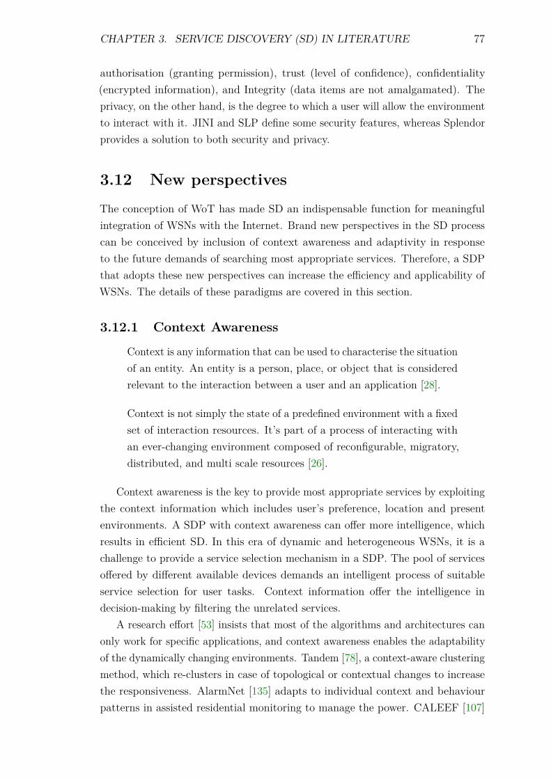
CHAPTER 3. SERVICE DISCOVERY (SD) IN LITERATURE 77
authorisation (granting permission), trust (level of confidence), confidentiality(encrypted information), and Integrity (data items are not amalgamated). Theprivacy, on the other hand, is the degree to which a user will allow the environmentto interact with it. JINI and SLP define some security features, whereas Splendorprovides a solution to both security and privacy.
3.12 New perspectives
The conception of WoT has made SD an indispensable function for meaningfulintegration of WSNs with the Internet. Brand new perspectives in the SD processcan be conceived by inclusion of context awareness and adaptivity in responseto the future demands of searching most appropriate services. Therefore, a SDPthat adopts these new perspectives can increase the efficiency and applicability ofWSNs. The details of these paradigms are covered in this section.
3.12.1 Context Awareness
Context is any information that can be used to characterise the situationof an entity. An entity is a person, place, or object that is consideredrelevant to the interaction between a user and an application [28].
Context is not simply the state of a predefined environment with a fixedset of interaction resources. It’s part of a process of interacting withan ever-changing environment composed of reconfigurable, migratory,distributed, and multi scale resources [26].
Context awareness is the key to provide most appropriate services by exploitingthe context information which includes user’s preference, location and presentenvironments. A SDP with context awareness can offer more intelligence, whichresults in efficient SD. In this era of dynamic and heterogeneous WSNs, it is achallenge to provide a service selection mechanism in a SDP. The pool of servicesoffered by different available devices demands an intelligent process of suitableservice selection for user tasks. Context information offer the intelligence indecision-making by filtering the unrelated services.
A research effort [53] insists that most of the algorithms and architectures canonly work for specific applications, and context awareness enables the adaptabilityof the dynamically changing environments. Tandem [78], a context-aware clusteringmethod, which re-clusters in case of topological or contextual changes to increasethe responsiveness. AlarmNet [135] adapts to individual context and behaviourpatterns in assisted residential monitoring to manage the power. CALEEF [107]
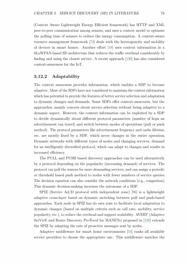
CHAPTER 3. SERVICE DISCOVERY (SD) IN LITERATURE 78
(Context Aware Lightweight Energy Efficient framework) has HTTP and XMLpeer-to-peer communication among sensors, and uses a context model to optimisethe polling time of sensors to reduce the energy consumption. A context-awareresource management framework [73] deals with the heterogeneity and mobilityof devices in smart homes. Another effort [19] uses context information in a6LoWPAN-based SD architecture that reduces the traffic overhead considerably byfinding and using the closest service. A recent approach [130] has also consideredcontext-awareness for the IoT.
3.12.2 Adaptability
The context awareness provides information, which enables a SDP to becomeadaptive. Most of the SDPs have not considered to maintain the context informationwhich has potential to provide the features of better service selection and adaptationto dynamic changes and demands. Some SDPs offer context-awareness, but theapproaches, mainly concern about service selection without being adaptive to adynamic aspect. However, the context information can be exploited by a SDPto decide dynamically about different protocol parameters (number of hops anadvertisement can travel) and switch between modes of operations (pull or pushmethod). The protocol parameters like advertisement frequency and cache lifetime,etc. are mostly fixed by a SDP, which never changes in the entire operation.Dynamic networks with different types of nodes and changing services, demandfor an intelligently diversified protocol, which can adapt to changes and results inincreased efficiency.
The PULL and PUSH based discovery approaches can be used alternativelyby a protocol depending on the popularity (increasing demand) of services. Theprotocol can poll the sensors for more demanding services, and can assign a periodicor threshold based push method to nodes with fewer numbers of service queries.The decision equation can also consider the network conditions (e.g., congestion).This dynamic decision-making increases the autonomy of a SDP.
SPIZ (Service Ad/D protocol with independent zone) [96] is a lightweightadaptive cross-layer based on dynamic switching between pull and push-basedapproaches. Each node in SPIZ has its own zone to facilitate local adaptation todynamic changes (based on multiple criteria such as call rate, mobility, servicepopularity, etc.), to reduce the overhead and support scalability. AVERT (AdaptiveSerVicE and Route Discovery ProTocol for MANETs) proposed in [128] extendsthe SPIZ by adapting the rate of proactive messages sent by nodes.
Adaptive middleware for smart home environments [54] ranks all availableservice providers to choose the appropriate one. This middleware matches the
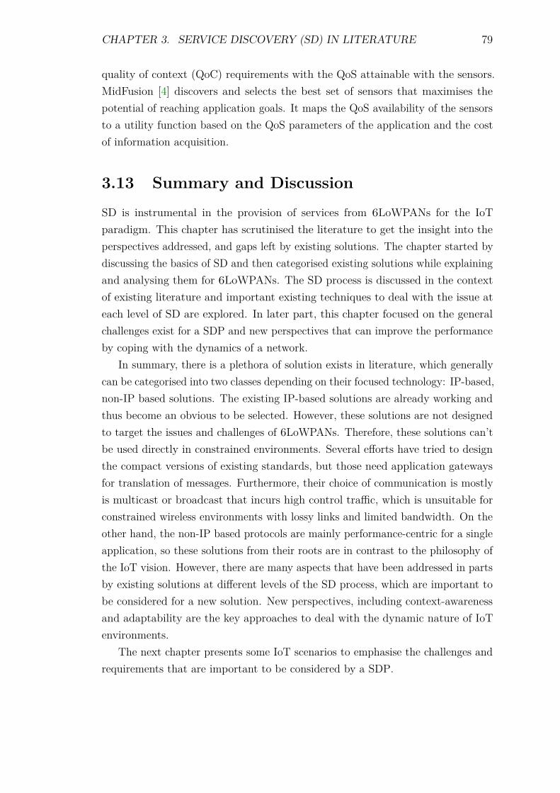
CHAPTER 3. SERVICE DISCOVERY (SD) IN LITERATURE 79
quality of context (QoC) requirements with the QoS attainable with the sensors.MidFusion [4] discovers and selects the best set of sensors that maximises thepotential of reaching application goals. It maps the QoS availability of the sensorsto a utility function based on the QoS parameters of the application and the costof information acquisition.
3.13 Summary and Discussion
SD is instrumental in the provision of services from 6LoWPANs for the IoTparadigm. This chapter has scrutinised the literature to get the insight into theperspectives addressed, and gaps left by existing solutions. The chapter started bydiscussing the basics of SD and then categorised existing solutions while explainingand analysing them for 6LoWPANs. The SD process is discussed in the contextof existing literature and important existing techniques to deal with the issue ateach level of SD are explored. In later part, this chapter focused on the generalchallenges exist for a SDP and new perspectives that can improve the performanceby coping with the dynamics of a network.
In summary, there is a plethora of solution exists in literature, which generallycan be categorised into two classes depending on their focused technology: IP-based,non-IP based solutions. The existing IP-based solutions are already working andthus become an obvious to be selected. However, these solutions are not designedto target the issues and challenges of 6LoWPANs. Therefore, these solutions can’tbe used directly in constrained environments. Several efforts have tried to designthe compact versions of existing standards, but those need application gatewaysfor translation of messages. Furthermore, their choice of communication is mostlyis multicast or broadcast that incurs high control traffic, which is unsuitable forconstrained wireless environments with lossy links and limited bandwidth. On theother hand, the non-IP based protocols are mainly performance-centric for a singleapplication, so these solutions from their roots are in contrast to the philosophy ofthe IoT vision. However, there are many aspects that have been addressed in partsby existing solutions at different levels of the SD process, which are important tobe considered for a new solution. New perspectives, including context-awarenessand adaptability are the key approaches to deal with the dynamic nature of IoTenvironments.
The next chapter presents some IoT scenarios to emphasise the challenges andrequirements that are important to be considered by a SDP.
Chapter 4
Service Discovery for the IoT: ARequirement Analysis
4.1 Introduction
The IoT vision integrates heterogeneous devices and networks together to form a newcollaborative paradigm. This creates new opportunities for co-ordination of end-to-end communication between devices from diverse networks. The idea of wrappingup a functionality into service and providing an interoperable way for invocationrevolutionises our perception regarding isolated constrained networks. SD playsa key role to assist the applications and users to locate services. However, thereare many challenges that are needed to be considered while devising any solutionfor IoT environments. The complexity is caused by the inherent diversity, whichdemands for the trade-off between generality (to deal with range of applications,devices and networks) and efficiency (for constrained domains). This requires aframework that should be evolvable to embrace the new challenges.
This chapter introduces some use-case scenarios in a IoT environment andhighlights the involved challenges and requirements.
4.2 Scenario
This section explains different scenarios to emphasise and analyse the role of SDsolution for the IoT paradigm. Firstly, this section covers the context of scenariosto give an overview of the situation.
Ipswich university (fictional) has transformed its traditional campus to anintelligent and automated one by installing new sensors in every building and room.The University has also created and distributed an application, to enable its staffand students to use features according to their defined authority. Furthermore,
80
CHAPTER 4. SD REQUIREMENT ANALYSIS FOR THE IOT 81
the application is smart enough to use the sensors on hand-held devices of usersto provide sensing information in a region. It also allows other user applications(personal management applications) to get access into the system. The wholesystem empowers the users to utilise functions ranging from finding the parkingspace to automate closing down their office windows.
Their system uses different policies to balance the trade-off between the networkoverhead and the prompt provision of services, depending on the time and demand.During the day in term time, system is scheduled to run on a full mode. This modeis more focused on reducing the delay time of SD and invocation. In the term’snight mode, system follows the security mode which only focuses on decreasingthe system overhead while providing the security breach alerts. The system alsohas scheduled off-peak policies for weekends and holidays. Furthermore, it allowsa power-user to add/amend policies depending on the current needs, e.g., in thecase of some emergency, etc.
Following are few situations where different users utilise the network:
Auto management of personal places with preferences: Michael is a seniorlecturer in Ipswich University. He spends time mostly in any of his two offices,and in his house. His mobile usually alerts him on reception of new emails,SMS, and tweets. He has installed the provided application to use featuresof his University’s smart system. He uses it to schedule the heating systemof his office, to get the alerts of opened windows, and to actuate set of tasksthat are performed on occurrence of some event (he is coming or leavingoffice). However, he is more interested in controlling his house in the sameway.
He installs “My iplaces” application, which allows him to save and view hiscommon places. The system of university authorises his application to log inand acquire various services as a registered user. The application allows himto see different status, e.g., temperature values and doors open/close. He canalso set alarms based on various rules specified by him. In addition, he cancreate sets of commands to execute e.g., When no one is at home close allwindows and notify me on security breach, etc. He can automate the wholeprocedure (e.g., leaving home) as well by allowing application to execute thecommands using his context, including current time and his GPS location.
Michael has different demands when he is at home. His home lights arealready intelligent enough to switch on when any motion is detected. However,he is more interested to adapt to current available light of a room to adjusttheir brightness using light sensor and only switching on when he is around.He has also specified different commands comprising a set of tasks, e.g., Set
CHAPTER 4. SD REQUIREMENT ANALYSIS FOR THE IOT 82
cinema environment command adjusts the blinds and lights, and changesthe TV settings. The application enables him to add any place, e.g., vehicle,garden, study room, bedroom, etc. and to browse through the availableservices in those areas to create set of commands.
Monitoring and management of places: Mark is a security personnel in IpswichUniversity. He has installed the University’s application on his phone. Uni-versity’s system allows mark to get security related alerts. It recognises himas a power user and allows him to load and change the policies based ondifferent circumstances.
Assisting users to find the best matched services: George is visiting the IpswichUniversity. He uses his “My iplaces” application to discover and add theIpswich University into his list. He logs in as a guest and tries to find thenearest parking space by giving his GPS location. Then he enters a buildingfor his meeting and searches for available printers around. He selects theclosest printer and issues a command to it.
4.3 User Interactions
The framework of the solution is required to support following three interactionmodels to materialise the discussed scenarios.
Direct interaction: Applications or users directly access sensors and actuators(in a server/client request-response model). In all scenarios, user applicationsneed to interact with the host devices to actuate a command.
Continuous monitoring: A continuous stream of data is required at regularintervals (e.g., Smart meters). This kind of interaction is required wherea user needs to monitor some sensed data, as for security personnel in thescenario.
Conditional monitoring: The updates are only sent when certain thresholdsare surpassed or some predefined event happens (e.g., temperature alerts).This is a requirement for Scenarios 1 and 2, where user needs to be notifiedon occurrence of some event.
4.4 IoT Service Discovery Requirements
The new IoT scenarios (Section 4.2) present a paradigm, where the plethora ofapplications discovers and invokes services hosted by IP-enabled smart devices.
CHAPTER 4. SD REQUIREMENT ANALYSIS FOR THE IOT 83
The SD solution needs to deal with a wide variety of devices ranging from very con-strained capabilities (e.g., RFID tags, sensor nodes) to resourceful ones (e.g., smartphones, printers, etc.). This section explains SD requirements extracted from thescenarios.
4.4.1 Heterogeneity and Interoperability
Following are some points in the context of inherent heterogeneity of the IoT andrequired interoperability:
• The system consists of heterogeneous devices and new devices can be integ-rated into the system as well. Consequently, the solution should not assumeanything about the involved hardware and allow the range of different devicesto be a part of it.
• Interoperability becomes crucial because of the underlying diversity. Thus, aSD solution should offer standard interface for services. Furthermore, solutionshould be routing and MAC protocol independent to allow the underlyingnetworks to select the one which suits them.
• The solution should accept service description ranging from very simple URLsto more concise form of XML or JSON descriptions.
• The devices can be mobile as well, so solution should specify a way to registerexplicit detail of device’s mobility to deal with them in a different manner.
4.4.2 Context-awareness
Context-awareness is an important factor to be considered in the IoT paradigm [100].The scenarios have emphasised the need of context-awareness, as each user isinterested to find services depending on his/her location. The challenge is to allowusers to discover more relevant and appropriate services based on the availablecontext information in a transparent manner. Following are the key requirementsgathered from the IoT use case scenarios:
• The solution should allow the user to search a service depending on somespecified context. There are different perspectives of context, e.g., relatednessdepending on location and user authority, battery, demand of service, etc.
• The minimum context information should include location. This can aid theuser application to define a query to discover a service in the proximity or ina specific location.
CHAPTER 4. SD REQUIREMENT ANALYSIS FOR THE IOT 84
• A service selection mechanism should be offered where in case of discovery ofmultiple services, a user seek assistance in the selection of an appropriate one.The benefits of service selection are many: it aids the user application to geta best matched service and it also enables the efficient usage of resourcese.g., by choosing the closest service in terms of number of hops.
• The solution can make the process even more efficient by saving the usercontext; for example, usual interest of an individual user to offer relatedservices. This can enable the solution to recognise the multiple requests fromusers and can adaptively facilitate them.
4.4.3 Adaptability
An adaptive SDP can tackle several challenges by adapting to dynamics of thenetwork to change different parameters, e.g., status maintenance interval, etc.The discussed scenarios introduced the concept of configuration profiles (set ofattributes), which can be changed by an adaptive solution dynamically w.r.t.current usage of a network. Following list recognises some of the potential adaptivefeatures that a SDP can provide:
• In SD, status maintenance overhead is a burden on the network that can bemarginalised by adapting to the current demand of a network.
• The solution can allow adaptive caching, so service invocation delay canbe reduced by using cached values. Constrained networks can be easilyoverwhelmed by the high number of invocations; therefore, in these networksthe energy and bandwidth can also be saved by providing the cached valuesfor services in high demand.
• The solution can allow to schedule and run different policies and configurationsbased on the dynamics of a network.
4.4.4 Constrained networks
The 6LoWPAN standard enables constrained networks to become an active partof the Internet. However, this also increases the number of challenges involved indesigning a solution for constrained networks. This section explains the constraintsthat should be considered by a SD solution for 6LoWPANs.
Scalability: The solution which can manage and control discovery overhead in adense network, while keeping track of the availability of service hosts.
CHAPTER 4. SD REQUIREMENT ANALYSIS FOR THE IOT 85
Compact size: The complexity of the solution should be implementable on theresource-constrained devices.
Compact communication: The limited bandwidth (20kbps to 250 kbps) andpacket size (127 bytes and 60-80 bytes) at the application layer of 6LoWPANs,demands a careful use of bandwidth. Large packets will get fragmented andresult in multiple packets, which can overwhelm the entire network.
Sleeping nodes: Constrained nodes usually save their limited power sources bysleeping most of the time, using a RDC. The solution should assign highpriority to this issue, by giving some alternatives like proxy which can act onbehalf of sleeping nodes.
Interoperability: Different standards for lower layers are being used in 6LoWPANs.The solution should be inter-operable to work between networks with di-verse standards. Interoperability aids the application development, as singleapplication can be used across different networks.
Energy efficiency: This is the key to increasing the lifetime of the network. Thesolution should optimise its operation by minimizing its control overhead.Furthermore, most of the nodes in multi-hop networks waste their energy bypassing the message towards the sink.
Resource-awareness: The assumptions of multiple resource-rich devices shouldnot be forced. However, the protocol should be opportunistic enough toexploit the availability of high-capacity devices .
Service composition: Many services are discovered and invoked together, mostlydepending on their vicinity. For example, switching lights on and off in aroom will require all the actuators of lights to be called collectively. A SDPshould consider this aspect to allow grouping of different services in a locality,to offer new services.
4.5 Summary
The analysis of the IoT requirements for SD provide the basis to propose an efficientsolution for this emerging domain. This chapter covered these requirements inthe context of future use-case scenarios. Furthermore, the application paradigmsand different user interactions are also explained to elaborate the points for auser oriented design of a SD solution. The requirement analysis has given moreemphasis to the needs of 6LoWPANs by explaining the implicit challenges of this

CHAPTER 4. SD REQUIREMENT ANALYSIS FOR THE IOT 86
constrained sub-domain of the IoT. The chapter is concluded by summarising thedesign choices for a SD solution with the future needs for IoT environments.
The next chapter discusses the first contribution, a context-aware SDP for theIoT, proposed by this research project.
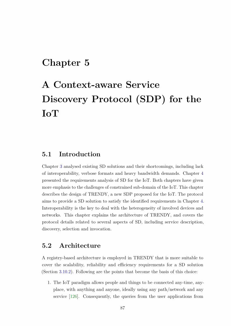
Chapter 5
A Context-aware ServiceDiscovery Protocol (SDP) for theIoT
5.1 Introduction
Chapter 3 analysed existing SD solutions and their shortcomings, including lackof interoperability, verbose formats and heavy bandwidth demands. Chapter 4presented the requirements analysis of SD for the IoT. Both chapters have givenmore emphasis to the challenges of constrained sub-domain of the IoT. This chapterdescribes the design of TRENDY, a new SDP proposed for the IoT. The protocolaims to provide a SD solution to satisfy the identified requirements in Chapter 4.Interoperability is the key to deal with the heterogeneity of involved devices andnetworks. This chapter explains the architecture of TRENDY, and covers theprotocol details related to several aspects of SD, including service description,discovery, selection and invocation.
5.2 Architecture
A registry-based architecture is employed in TRENDY that is more suitable tocover the scalability, reliability and efficiency requirements for a SD solution(Section 3.10.2). Following are the points that become the basis of this choice:
1. The IoT paradigm allows people and things to be connected any-time, any-place, with anything and anyone, ideally using any path/network and anyservice [126]. Consequently, the queries from the user applications from
87
CHAPTER 5. SDP FOR THE IOT 88
outside the network is the norm in such environments. This requires a placeto deal with these queries, and certainly a directory-based approach will servethe purpose.
2. This architecture is a better match for 6LoWPANs, where nodes mostlysleep, and broadcasting or multicasting is an expensive way to discover aservice in the case of a directory-less solution (Section 3.10.2).
Figure 5.1 presents TRENDY’s architecture. It consists of: the DA (DirectoryAgent), SAs (Service Agents) and UAs (User Agents). This section further coversthe detail of these entities.
��
��
������� � ���
��
�� ��
��
��
������� � ���
��
�� ��
��
��
������� �����
��
��
��
��
�� ����������������
������
�
�����
���
�� �� ��
Figure 5.1: Architecture of TRENDY
5.2.1 Directory Agent (DA)
The DA has a backbone role in TRENDY’s architecture and serves followingresponsibilities:
• Registry: The DA maintains a registry table to store soft state entries forregistered services and context information by the host devices.
• Status maintenance: All registry entries bound to a lifetime period spe-cified by the size of the DA’s time window. Host devices need to update theirstatus at the DA or their entries are deleted to ensure reliability.
• Service discovery and selection: The DA responds to SD requests anduses collected context information to select a better service.
CHAPTER 5. SDP FOR THE IOT 89
• Service Invocation: The DA can act optionally as a proxy, in this case itwill respond on behalf of other devices and other benefits like caching canalso be exploited.
5.2.2 Service Agent (SA)
A SA is any host device that registers its service descriptions and context inform-ation at the DA. It receives a time window length in response to a registrationmessage, which specifies the maximum time to send a status update to the DA.All SAs need to keep the DA updated about their availability by sending statusupdates within a time window.
5.2.3 User Agent (UA)
A UA is a client interested in discovering services available . It sends discoveryrequests to the DA, and can be located either within a sensor network or elsewherein the Internet.
5.3 Communication Protocol
The RESTful web service paradigm is more suitable for embedded constrainednetworks because of its simplicity and efficiency (Section 2.4.4.2). Furthermore,CoAP (Section 2.5) is a compact and interoperable alternative to HTTP and can beutilised to enable this paradigm in constrained networks [25]. Therefore, CoAP isemployed by TRENDY as a default communication protocol between devices. AllSAs and UAs can communicate with the DA using either CoAP (default) or HTTP.However, SAs in constraint networks such as 6LoWPANs will require proxies tooffer interoperability to HTTP. Moreover, the DA can be extended to present itsservices in other formats (depending on its capability) and can respond to queriessent using other protocols e.g., DNS-SD.
5.4 Service Description
Service descriptions are important to provide a better SD by giving a more detail fora service. In the IoT, there can be diverse requirements on the level of informationneeded to be specified by the devices depending on the context of the applicationand capabilities of the devices. There are several possible service types that canbe used by the IoT applications. This suggests the need for such a solution thatcan accept different service descriptions ranging from very brief to semantically
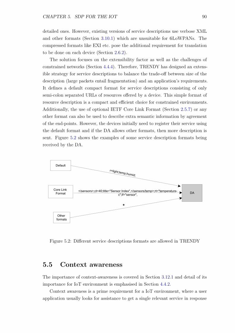
CHAPTER 5. SDP FOR THE IOT 90
detailed ones. However, existing versions of service descriptions use verbose XMLand other formats (Section 3.10.1) which are unsuitable for 6LoWPANs. Thecompressed formats like EXI etc. pose the additional requirement for translationto be done on each device (Section 2.6.2).
The solution focuses on the extensibility factor as well as the challenges ofconstrained networks (Section 4.4.4). Therefore, TRENDY has designed an extens-ible strategy for service descriptions to balance the trade-off between size of thedescription (large packets entail fragmentation) and an application’s requirements.It defines a default compact format for service descriptions consisting of onlysemi-colon separated URLs of resources offered by a device. This simple format ofresource description is a compact and efficient choice for constrained environments.Additionally, the use of optional IETF Core Link Format (Section 2.5.7) or anyother format can also be used to describe extra semantic information by agreementof the end-points. However, the devices initially need to register their service usingthe default format and if the DA allows other formats, then more description issent. Figure 5.2 shows the examples of some service description formats beingreceived by the DA.
��
�������
�� � ������
���������
�� ������������ ��
���������������� ���� !��� "���# $���������������� ���������%� � �� ���� $
�
Figure 5.2: Different service descriptions formats are allowed in TRENDY
5.5 Context awareness
The importance of context-awareness is covered in Section 3.12.1 and detail of itsimportance for IoT environment is emphasised in Section 4.4.2.
Context awareness is a prime requirement for a IoT environment, where a userapplication usually looks for assistance to get a single relevant service in response
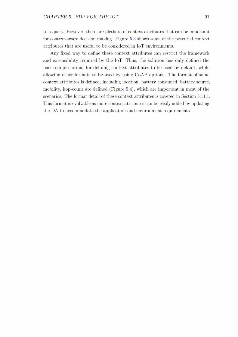
CHAPTER 5. SDP FOR THE IOT 91
to a query. However, there are plethora of context attributes that can be importantfor context-aware decision making. Figure 5.3 shows some of the potential contextattributes that are useful to be considered in IoT environments.
Any fixed way to define these context attributes can restrict the frameworkand extensibility required by the IoT. Thus, the solution has only defined thebasic simple format for defining context attributes to be used by default, whileallowing other formats to be used by using CoAP options. The format of somecontext attributes is defined, including location, battery consumed, battery source,mobility, hop-count are defined (Figure 5.4), which are important in most of thescenarios. The format detail of these context attributes is covered in Section 5.11.1.This format is evolvable as more context attributes can be easily added by updatingthe DA to accommodate the application and environment requirements.
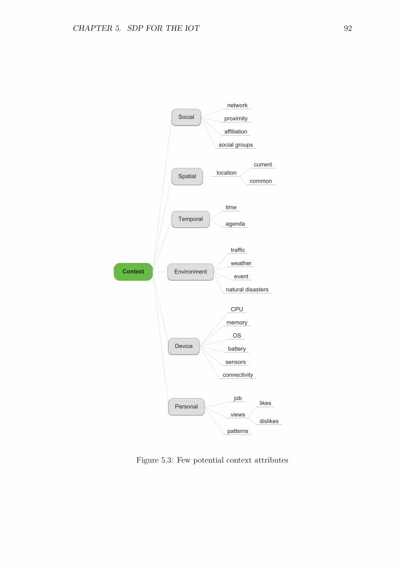
CHAPTER 5. SDP FOR THE IOT 92
�������
������
�����
�� �����
�����������
������ �����
������� �������������
������
�������
����
������
����������
����
�����
���������������
���������������
�����
������
������ ��������
������
���
�����
�
������
������
������������
Figure 5.3: Few potential context attributes
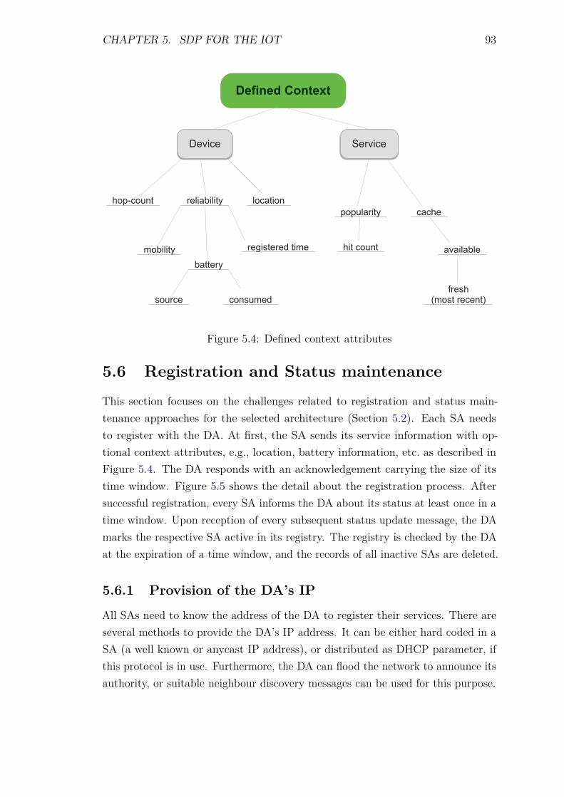
CHAPTER 5. SDP FOR THE IOT 93
������� ����
�������
�����
��������
���� ���� �������
����������
��� �����
������
��������� ����������
���������� ����
������
��������������
�������
��������
Figure 5.4: Defined context attributes
5.6 Registration and Status maintenance
This section focuses on the challenges related to registration and status main-tenance approaches for the selected architecture (Section 5.2). Each SA needsto register with the DA. At first, the SA sends its service information with op-tional context attributes, e.g., location, battery information, etc. as described inFigure 5.4. The DA responds with an acknowledgement carrying the size of itstime window. Figure 5.5 shows the detail about the registration process. Aftersuccessful registration, every SA informs the DA about its status at least once in atime window. Upon reception of every subsequent status update message, the DAmarks the respective SA active in its registry. The registry is checked by the DAat the expiration of a time window, and the records of all inactive SAs are deleted.
5.6.1 Provision of the DA’s IP
All SAs need to know the address of the DA to register their services. There areseveral methods to provide the DA’s IP address. It can be either hard coded in aSA (a well known or anycast IP address), or distributed as DHCP parameter, ifthis protocol is in use. Furthermore, the DA can flood the network to announce itsauthority, or suitable neighbour discovery messages can be used for this purpose.
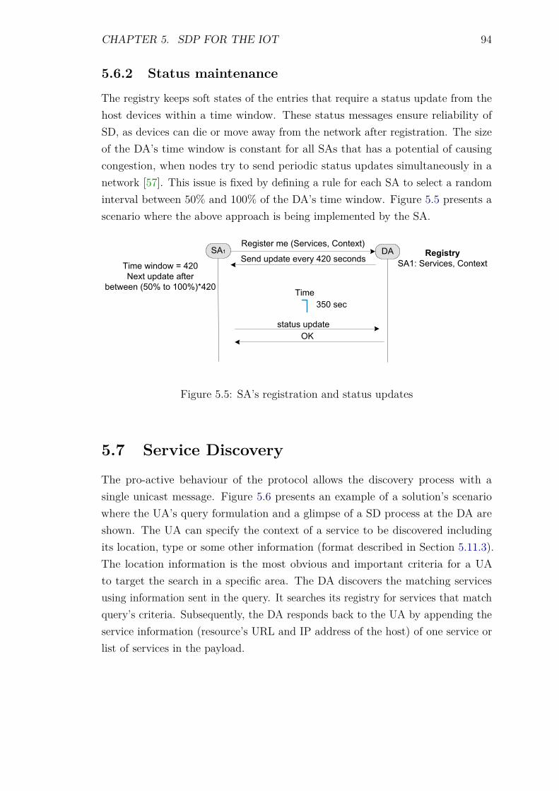
CHAPTER 5. SDP FOR THE IOT 94
5.6.2 Status maintenance
The registry keeps soft states of the entries that require a status update from thehost devices within a time window. These status messages ensure reliability ofSD, as devices can die or move away from the network after registration. The sizeof the DA’s time window is constant for all SAs that has a potential of causingcongestion, when nodes try to send periodic status updates simultaneously in anetwork [57]. This issue is fixed by defining a rule for each SA to select a randominterval between 50% and 100% of the DA’s time window. Figure 5.5 presents ascenario where the above approach is being implemented by the SA.
��� �������� �� �������� ������
���� ����� ���� ��� ����������� ������ ���"�� ����� �#�
$����� %�& � ���&�'��� ����
()���� �����
*%� ���
�����������+ �������� �����
Figure 5.5: SA’s registration and status updates
5.7 Service Discovery
The pro-active behaviour of the protocol allows the discovery process with asingle unicast message. Figure 5.6 presents an example of a solution’s scenariowhere the UA’s query formulation and a glimpse of a SD process at the DA areshown. The UA can specify the context of a service to be discovered includingits location, type or some other information (format described in Section 5.11.3).The location information is the most obvious and important criteria for a UAto target the search in a specific area. The DA discovers the matching servicesusing information sent in the query. It searches its registry for services that matchquery’s criteria. Subsequently, the DA responds back to the UA by appending theservice information (resource’s URL and IP address of the host) of one service orlist of services in the payload.
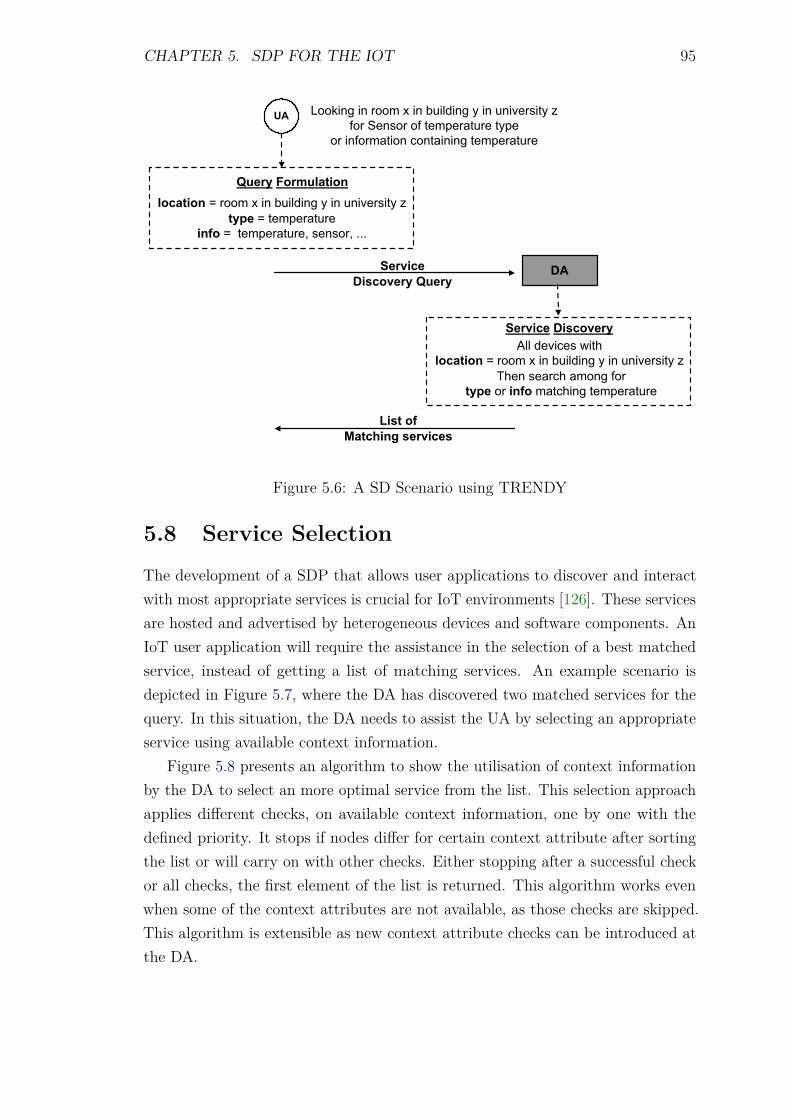
CHAPTER 5. SDP FOR THE IOT 95
��
����� ��������
��
��������������� �����
������� �� ���� �� ��� ��� � �� ���������� ���� ������ �� ����������� ����
�� ����������� ���������� �����������
�������� � ���� �� ��� ��� � �� ���������� ����� � �����������
���� � ������������ ������� ���
������� ������������ ������ ����
�������� � ���� �� ��� ��� � �� ���������� � ��� ������ ����� ���
���� �� ���� �������� �����������
��� ���������� ������
Figure 5.6: A SD Scenario using TRENDY
5.8 Service Selection
The development of a SDP that allows user applications to discover and interactwith most appropriate services is crucial for IoT environments [126]. These servicesare hosted and advertised by heterogeneous devices and software components. AnIoT user application will require the assistance in the selection of a best matchedservice, instead of getting a list of matching services. An example scenario isdepicted in Figure 5.7, where the DA has discovered two matched services for thequery. In this situation, the DA needs to assist the UA by selecting an appropriateservice using available context information.
Figure 5.8 presents an algorithm to show the utilisation of context informationby the DA to select an more optimal service from the list. This selection approachapplies different checks, on available context information, one by one with thedefined priority. It stops if nodes differ for certain context attribute after sortingthe list or will carry on with other checks. Either stopping after a successful checkor all checks, the first element of the list is returned. This algorithm works evenwhen some of the context attributes are not available, as those checks are skipped.This algorithm is extensible as new context attribute checks can be introduced atthe DA.
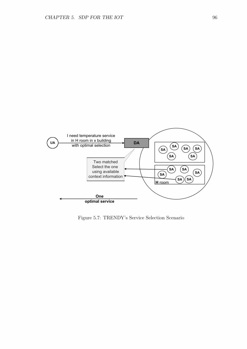
CHAPTER 5. SDP FOR THE IOT 96
����
� ���� ��������� ���� �� � � ���� � � � �� ��� �� ��� �� ������ ��
������� ������
���� �� ��
�� ��
���� ��
��
�� ��� ����
��� ������������ ��� ���� �� � ����
������� ������ ��
Figure 5.7: TRENDY’s Service Selection Scenario
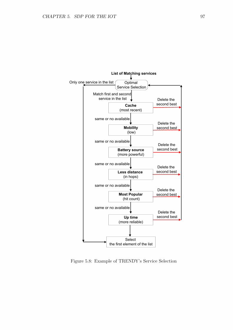
CHAPTER 5. SDP FOR THE IOT 97
���������� � ����
���������� � ���
�����������
��� � ��� ������ ��������
���� ���������� �����
��� ����� ���� �����
�� ������� �������
��� �� ������� �� �����
��� �� �� ��������
��� ��� ��� ���
� ��� ����� ���� �� �� ����
��� � ����� ��� � ������� �� �� ����
��� �� �� ��������
��� �� �� ��������
��� �� �� ��������
��� �� �� ��������
��� ��� ��� ���
��� ��� ��� ���
��� ��� ��� ���
��� ��� ��� ���
��� ��� ��� ���
���� �� ���� �� �� ����
Figure 5.8: Example of TRENDY’s Service Selection
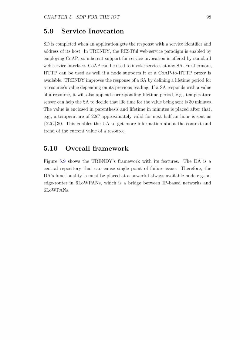
CHAPTER 5. SDP FOR THE IOT 98
5.9 Service Inovcation
SD is completed when an application gets the response with a service identifier andaddress of its host. In TRENDY, the RESTful web service paradigm is enabled byemploying CoAP, so inherent support for service invocation is offered by standardweb service interface. CoAP can be used to invoke services at any SA. Furthermore,HTTP can be used as well if a node supports it or a CoAP-to-HTTP proxy isavailable. TRENDY improves the response of a SA by defining a lifetime period fora resource’s value depending on its previous reading. If a SA responds with a valueof a resource, it will also append corresponding lifetime period, e.g., temperaturesensor can help the SA to decide that life time for the value being sent is 30 minutes.The value is enclosed in parenthesis and lifetime in minutes is placed after that,e.g., a temperature of 22C approximately valid for next half an hour is sent as{22C}30. This enables the UA to get more information about the context andtrend of the current value of a resource.
5.10 Overall framework
Figure 5.9 shows the TRENDY’s framework with its features. The DA is acentral repository that can cause single point of failure issue. Therefore, theDA’s functionality is must be placed at a powerful always available node e.g., atedge-router in 6LoWPANs, which is a bridge between IP-based networks and6LoWPANs.
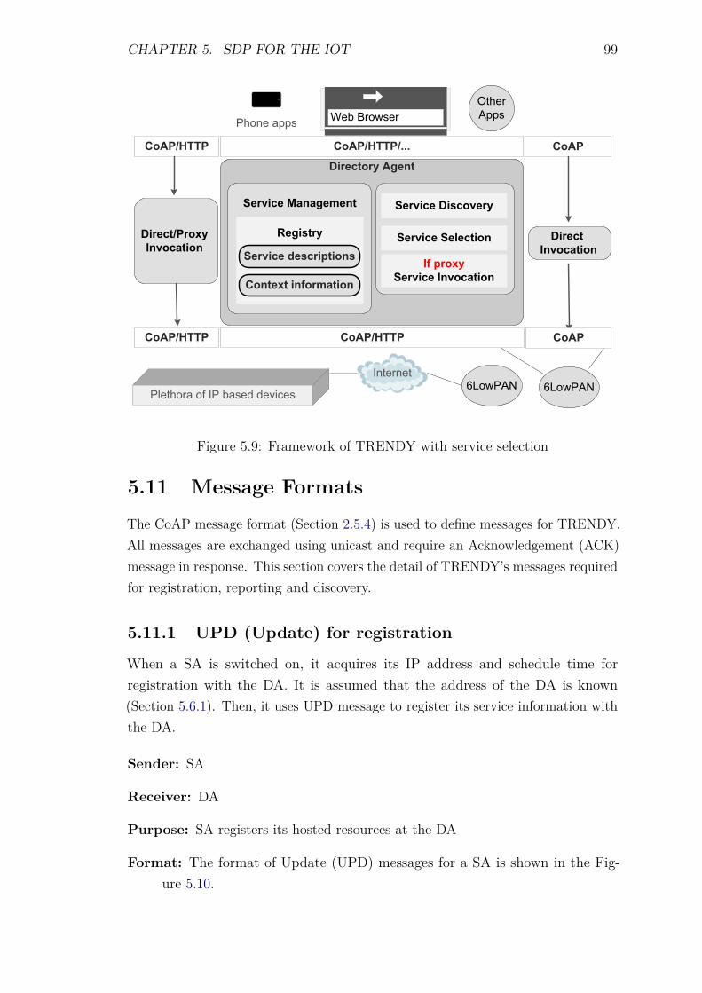
CHAPTER 5. SDP FOR THE IOT 99
��������� ���
��� ���������� ��
��������������
������ �� � � �� ������
��������
�������
������� ��������� ������� ���������
������� �������������������������������
��
����������������
������
�����������
������� �� �������
�������
�� ������������ ����������
������� ������������
������ �����������
Figure 5.9: Framework of TRENDY with service selection
5.11 Message Formats
The CoAP message format (Section 2.5.4) is used to define messages for TRENDY.All messages are exchanged using unicast and require an Acknowledgement (ACK)message in response. This section covers the detail of TRENDY’s messages requiredfor registration, reporting and discovery.
5.11.1 UPD (Update) for registration
When a SA is switched on, it acquires its IP address and schedule time forregistration with the DA. It is assumed that the address of the DA is known(Section 5.6.1). Then, it uses UPD message to register its service information withthe DA.
Sender: SA
Receiver: DA
Purpose: SA registers its hosted resources at the DA
Format: The format of Update (UPD) messages for a SA is shown in the Fig-ure 5.10.
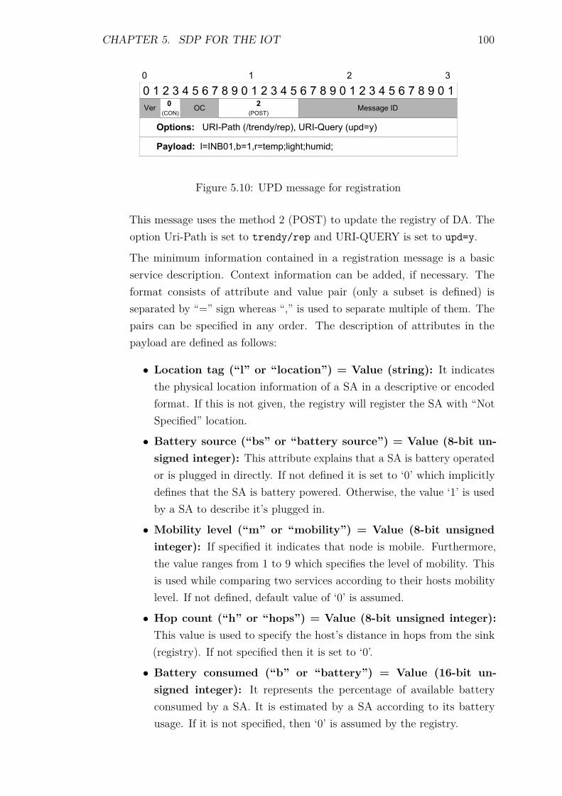
CHAPTER 5. SDP FOR THE IOT 100
� � � � � � � � � � � � � � � � � � � � � � � � � ��� ��
�������� �������� ��� ����� ���� ���� !� � �!��"��
����� #"�$%���&"�� "��'�(#)*��(�!')�(
� � � �
���$�
����-.�
/�00�*� �1
Figure 5.10: UPD message for registration
This message uses the method 2 (POST) to update the registry of DA. Theoption Uri-Path is set to trendy/rep and URI-QUERY is set to upd=y.
The minimum information contained in a registration message is a basicservice description. Context information can be added, if necessary. Theformat consists of attribute and value pair (only a subset is defined) isseparated by “=” sign whereas “,” is used to separate multiple of them. Thepairs can be specified in any order. The description of attributes in thepayload are defined as follows:
• Location tag (“l” or “location”) = Value (string): It indicatesthe physical location information of a SA in a descriptive or encodedformat. If this is not given, the registry will register the SA with “NotSpecified” location.
• Battery source (“bs” or “battery source”) = Value (8-bit un-signed integer): This attribute explains that a SA is battery operatedor is plugged in directly. If not defined it is set to ‘0’ which implicitlydefines that the SA is battery powered. Otherwise, the value ‘1’ is usedby a SA to describe it’s plugged in.
• Mobility level (“m” or “mobility”) = Value (8-bit unsignedinteger): If specified it indicates that node is mobile. Furthermore,the value ranges from 1 to 9 which specifies the level of mobility. Thisis used while comparing two services according to their hosts mobilitylevel. If not defined, default value of ‘0’ is assumed.
• Hop count (“h” or “hops”) = Value (8-bit unsigned integer):This value is used to specify the host’s distance in hops from the sink(registry). If not specified then it is set to ‘0’.
• Battery consumed (“b” or “battery”) = Value (16-bit un-signed integer): It represents the percentage of available batteryconsumed by a SA. It is estimated by a SA according to its batteryusage. If it is not specified, then ‘0’ is assumed by the registry.
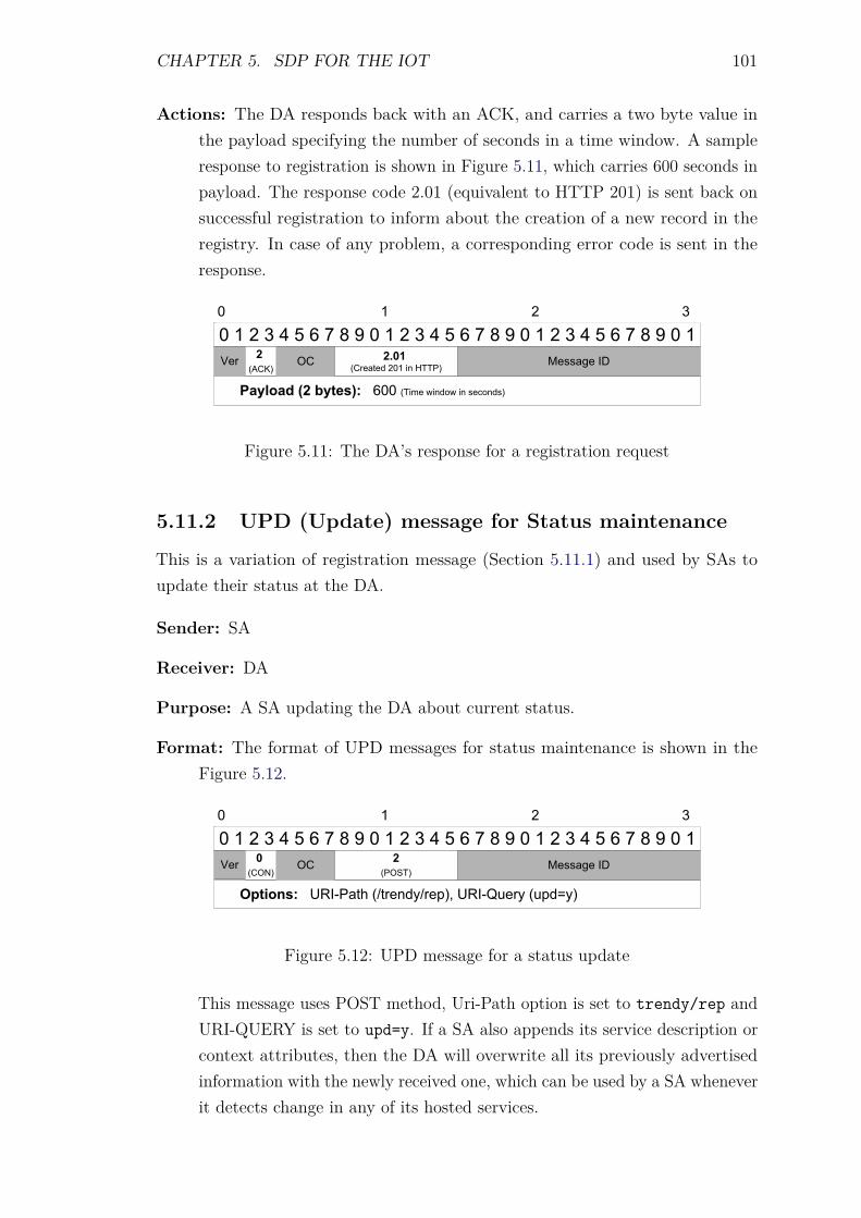
CHAPTER 5. SDP FOR THE IOT 101
Actions: The DA responds back with an ACK, and carries a two byte value inthe payload specifying the number of seconds in a time window. A sampleresponse to registration is shown in Figure 5.11, which carries 600 seconds inpayload. The response code 2.01 (equivalent to HTTP 201) is sent back onsuccessful registration to inform about the creation of a new record in theregistry. In case of any problem, a corresponding error code is sent in theresponse.
� � � � � � � � � � � � � � � � � � � � � � � � � ��� ��
������� �� ��� � ��� ����� ������ �� ��������
� � � �
������
������ �� �� ��� �� !��"� #����$� %&
Figure 5.11: The DA’s response for a registration request
5.11.2 UPD (Update) message for Status maintenance
This is a variation of registration message (Section 5.11.1) and used by SAs toupdate their status at the DA.
Sender: SA
Receiver: DA
Purpose: A SA updating the DA about current status.
Format: The format of UPD messages for status maintenance is shown in theFigure 5.12.
� � � � � � � � � � � � � � � � � � � � � � � � � ��� ��
�������� �������� ��� ����� ���� ���� !� � �!��"��
� � � �
����$�
���&'�
(�))�*� �+
Figure 5.12: UPD message for a status update
This message uses POST method, Uri-Path option is set to trendy/rep andURI-QUERY is set to upd=y. If a SA also appends its service description orcontext attributes, then the DA will overwrite all its previously advertisedinformation with the newly received one, which can be used by a SA wheneverit detects change in any of its hosted services.

CHAPTER 5. SDP FOR THE IOT 102
Actions: Figure 5.11 shows the format of an ACK. In the case of a successfulupdate, a response code 2.04 (equivalent to HTTP 204) is sent back. In caseof a failure, the DA will send a reset message with corresponding error code,as shown in Figure 5.13. After receiving such a reset message the SA willsend another UPD message for registration of its services at the DA.
� � � � � � � � � � � � � � � � � � � � � � � � � ��� ��
� � � �
������
������ � ��� �� �����
����� � !"
Figure 5.13: Reset response from the DA
5.11.3 SDR (Service Discovery Request)
This section covers the detail of Service Discovery Request (SDR) message whichis used by a UA to discover a service.
Sender: UA
Receiver: DA
Purpose: Services are maintained at the DA to enable a unicast discovery. TheDA accepts SDR messages in both CoAP (default) and HTTP protocol.The UA uses URL query options to explain context of a service or multipleservices to discover. Services are searched based on attached query attributesand responded accordingly.
Format: A UA specifies the trendy/server URL with CoAP’s GET method andURL queries (examples shown in Table 5.1) for SD. The discovery query canbe specified in one of the following three different ways:
1. Attribute-based: The UA can define type, info (information) andlocation attributes using URI-QUERY to describe a query. Any or allattributes can be used to discover a service. The format of this type isshown in Figure 5.14.
2. Best search based: Any attribute based discovery message can beamended by adding best in the payload to seek assistance from the DAfor appropriate service selection.
3. Other format request: The UA can request for the WSDL or WADLfile of service information, by mentioning a URI-QUERY option withthe format name. The message format is shown in Figure 5.15.
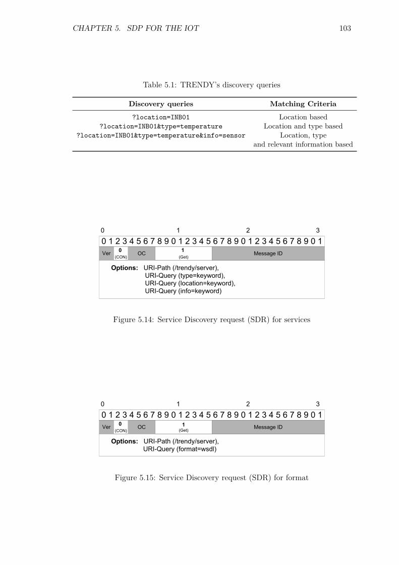
CHAPTER 5. SDP FOR THE IOT 103
Table 5.1: TRENDY’s discovery queries
Discovery queries Matching Criteria
?location=INB01 Location based?location=INB01&type=temperature Location and type based
?location=INB01&type=temperature&info=sensor Location, typeand relevant information based
� � � � � � � � � � � � � � � � � � � � � � � � � ��� ��
�������� �������� ��� ������� �� � ����#$� � ���%�&'��() �� ����#$� � �*)+��,)�&'��() �� ����#$� � �,�-)&'��() ��
� � � �
����.�
�/���
0����1� �2
Figure 5.14: Service Discovery request (SDR) for services
� � � � � � � � � � � � � � � � � � � � � � � � � ��� ��
�������� �������� ��� ������� �� � ����#$� � �%& '��()��*�
� � � �
����+�
�,��� -����.� �/
Figure 5.15: Service Discovery request (SDR) for format
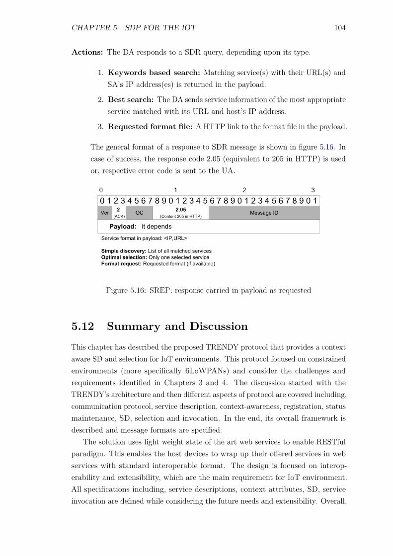
CHAPTER 5. SDP FOR THE IOT 104
Actions: The DA responds to a SDR query, depending upon its type.
1. Keywords based search: Matching service(s) with their URL(s) andSA’s IP address(es) is returned in the payload.
2. Best search: The DA sends service information of the most appropriateservice matched with its URL and host’s IP address.
3. Requested format file: A HTTP link to the format file in the payload.
The general format of a response to SDR message is shown in figure 5.16. Incase of success, the response code 2.05 (equivalent to 205 in HTTP) is usedor, respective error code is sent to the UA.
� � � � � � � � � � � � � � � � � � � � � � � � � ��� ��
�������� �� �������
� � � �
������
���������� ��� �� �����
���!"� #$
%� &�'� (� )!� �� �!*+�!�, -#�./012
� ���� � �������� 1��� �( !++ )!�'3�� �� &�'����� ��� ������ ��� ��+* ��� ��+�'��� �� &�'������� �������� 0�45����� (� )!� ��( !&!�+!6+��
Figure 5.16: SREP: response carried in payload as requested
5.12 Summary and Discussion
This chapter has described the proposed TRENDY protocol that provides a contextaware SD and selection for IoT environments. This protocol focused on constrainedenvironments (more specifically 6LoWPANs) and consider the challenges andrequirements identified in Chapters 3 and 4. The discussion started with theTRENDY’s architecture and then different aspects of protocol are covered including,communication protocol, service description, context-awareness, registration, statusmaintenance, SD, selection and invocation. In the end, its overall framework isdescribed and message formats are specified.
The solution uses light weight state of the art web services to enable RESTfulparadigm. This enables the host devices to wrap up their offered services in webservices with standard interoperable format. The design is focused on interop-erability and extensibility, which are the main requirement for IoT environment.All specifications including, service descriptions, context attributes, SD, serviceinvocation are defined while considering the future needs and extensibility. Overall,

CHAPTER 5. SDP FOR THE IOT 105
TRENDY offers a SD solution that satisfies new requirements of the IoT and morespecifically deals with the challenges posed by its constrained domains.
The next chapter explains the experimental design with the detail of selectedtools for experiments. Afterwards, Chapters 7, 8, 9 describe additional techniquesfor TRENDY including, adaptive timer, context-aware grouping and adaptivecaching.
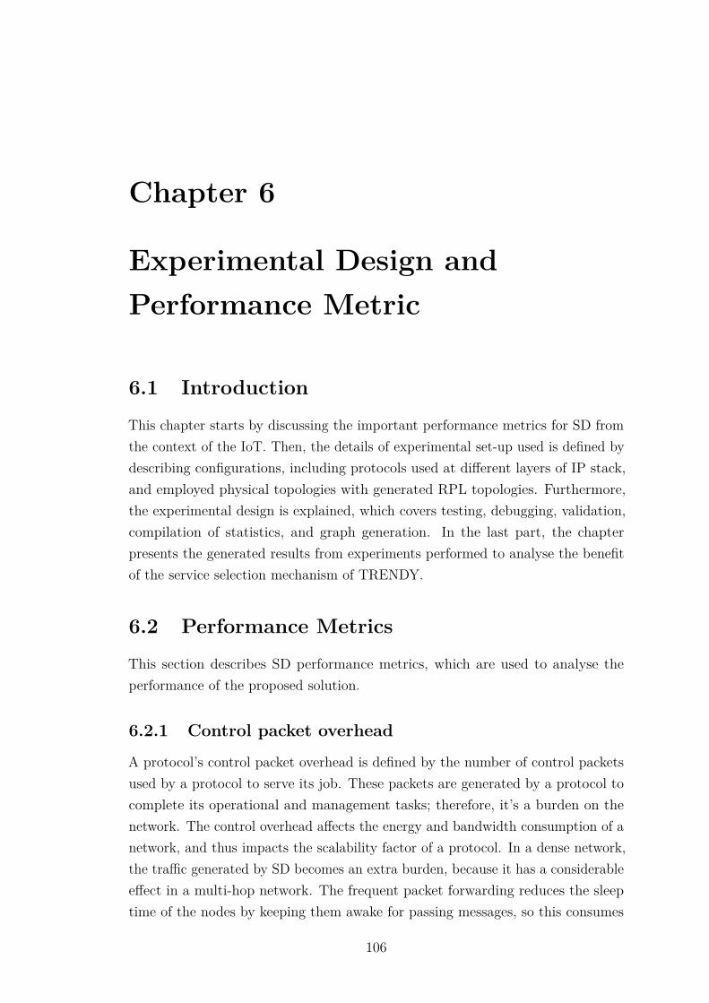
Chapter 6
Experimental Design andPerformance Metric
6.1 Introduction
This chapter starts by discussing the important performance metrics for SD fromthe context of the IoT. Then, the details of experimental set-up used is defined bydescribing configurations, including protocols used at different layers of IP stack,and employed physical topologies with generated RPL topologies. Furthermore,the experimental design is explained, which covers testing, debugging, validation,compilation of statistics, and graph generation. In the last part, the chapterpresents the generated results from experiments performed to analyse the benefitof the service selection mechanism of TRENDY.
6.2 Performance Metrics
This section describes SD performance metrics, which are used to analyse theperformance of the proposed solution.
6.2.1 Control packet overhead
A protocol’s control packet overhead is defined by the number of control packetsused by a protocol to serve its job. These packets are generated by a protocol tocomplete its operational and management tasks; therefore, it’s a burden on thenetwork. The control overhead affects the energy and bandwidth consumption of anetwork, and thus impacts the scalability factor of a protocol. In a dense network,the traffic generated by SD becomes an extra burden, because it has a considerableeffect in a multi-hop network. The frequent packet forwarding reduces the sleeptime of the nodes by keeping them awake for passing messages, so this consumes
106
CHAPTER 6. EXPERIMENTAL DESIGN 107
more energy. Therefore, an efficient and scalable SD solution generates less controltraffic.
In the case of TRENDY, an application layer protocol, the control overheadis the sum of all registration, and reporting messages. The number of serviceinvocation messages are technically not considered as a part of overhead; however,if a SDP employs a caching mechanism, then this number becomes important toanalyse the impact of the scheme.
TRENDY works at application layer and is independent of lower layer protocolsthat’s why only application-layer level packets are counted to calculate its overhead.However, in reality, the application layer messages initiate a round of several effortsat the bottom layers, and overhead actually costs several times more than thecount at the top layer. This effect becomes much larger for 6LoWPANs with lossyradio environments consist of nodes with sleeping cycles, as one packet might besent several times before it reaches at the destination. Therefore, the total networkpackets are also recorded in experiments to quantify the impact of such properties.Subsequently, further analysis is done on recorded packets using Wireshark [98] tosegregate and classify SD messages from routing and other messages.
6.2.2 Service Discovery Delay
The service discovery delay is the interval between initiation of a UA query messageand receipt of a response from the DA. It includes the processing time at the DAto match and select a service with query parameters. TRENDY has a registry-based architecture and has proactive behaviour, so this factor does not have muchsignificance because only a single uni-cast message required between two entities(UA and DA) for SD. However, it is an important SD metric that matters morein directory-less and distributed directory based solutions where a query has topass through different nodes either by multicast or unicast in case of multiple localdirectories.
6.2.3 Service Invocation Delay and cache hits
Service Invocation (SI) delay is defined by the time taken from issuing an invocationrequest until the receipt of a response. This is an important parameter to analysethe efficiency of a SD solution, because lower SI delay means better systemperformance and response to a user application. The network traffic load, averagepath length in multi-hop network and message processing time are the factors thataffect the SI delay. Usually, a service discovery solution has no impact on thismetric, unless it is either supporting service selection, service invocation or usingsome caching mechanism to facilitate user applications. If caching is enabled, then

CHAPTER 6. EXPERIMENTAL DESIGN 108
the number of cache hits defines the number of times the maintained cache is usedby the registry to serve a request. This number measures the benefit of maintainingthe cached values. TRENDY’s employed communication protocol; CoAP, enablesservice invocation using RESTful web services. Thus, service invocation delaybecomes an important metric to be measured in TRENDY experiments.
6.2.4 Energy Efficiency and Network lifetime
Energy is considered a precious resource in 6LoWPANs with mostly battery-operated nodes. A node consumes energy while processing, sleeping, and radiolistening, receiving and transmitting. Energy consumption is also highly dependenton the routing overhead, and selected MAC and RDC mechanisms [6].
In experiments, Energest [33] is used to evaluate the energy consumptionof individual nodes. Energest is a software-based mechanism to estimate theenergy consumption of a sensor node, which runs directly on a node to providereal-time estimates of current energy consumption. It keeps track of the timespent by individual modules, including, CPU, radio transceiver (listen, receivingand transmitting), and low power or sleep mode. The time is then processedusing the data-sheet of emulated devices to calculate the energy consumption.COOJA performs the simulations at the hardware-level by using the real hardwareprofiles of the employed nodes; therefore, devices can be emulated with actualhardware configurations. Tmote Sky motes are emulated in all experiments as6LoWPAN nodes in COOJA. Table 6.1 shows the data-sheet values of currentconsumed by a Tmote Sky while performing different operations. These valuesalong with CONTIKI’s fixed operating voltage of 3V are used in experiments tocalculate the total energy consumption of each node. Different statistics, including,individual node energy consumption and average node energy consumption areused to compare the energy efficiency of proposed techniques in the performedexperiments.
Table 6.1: Current consumed by a Tmote Sky while performing different operations
Operation Current(mAmp)
Radio listening and Receiving 19.7Radio transmit 17.4
CPU ON 1.95CPU LPM (Low Power Mode) 0.5
Energy consumption and network lifetime are interrelated as lower energyconsumption suggests that network will last longer. The definition of the network
CHAPTER 6. EXPERIMENTAL DESIGN 109
lifetime varies according to a specific application or topology [20]. In TRENDY,location tags are considered as a key criterion to search and differentiate servicesaccording to their placement within a network. Therefore, the network is segregatedinto different locations with a dynamic topology with the RPL [133] protocol. RPLmaintains its topology by forming new routes dynamically during the simulationperiod. Consequently, the different topologies are used in experiments to check theimpact of the diversity of generated RPL routing trees. In reality, the definition ofthe network lifetime depends upon the way nodes are placed in a network. Thisresearch project considers the most widely used definition of the network lifetimewhere the network lasts until first node dies in a network.
Emulated Tmote Sky motes can be powered by two AA batteries with operatingvoltage range between 2.1V to 3.6V . Normally, two Alkaline batteries provide onaverage capacity of 2500mAh with operating voltage of 3 volts. Following formulais used to compute the capacity of batteries in Joules.
ECapacity = V × I × 3600
Where ECapacity represents the available energy in Joules, V is the electromotiveforce expressed in volts and I is the current expressed in amperes. The equationV × I is multiplied by 3600 to get the Watt-seconds. Therefore, the total availableenergy capacity, by applying the formula is:
ECapacity = 2.5× 3× 3600
ECapacity = 27000 Joules
The individual energy consumption of nodes during a simulation period is usedto linearly approximate the energy required by them in a day, which is used furtherto approximate the total lifetime of nodes for available energy capacity providedby two AA batteries. The assumption taken here is that all batteries will provide2500mAh capacity while their voltage will never drop from 3 Volts. Finally, theseestimations are used to determine the time when first node dies.
The assumption taken in energy consumption approximations is that the sameevents occurred during the simulation period (number of UA queries and controloverhead) will keep on repeating in the similar way over the lifetime of the network.However, the nodes will not get registered again neither the equivalent numberof queries will be repeated in reality. For example, in the discussed scenarios(Section 4.2), the network is supposed to have longer idle periods of low demandduring the nights. Therefore, this calculation is only an assumption and representsan approximation of the network lifetime for a rather worst-case scenario.
CHAPTER 6. EXPERIMENTAL DESIGN 110
6.2.5 Scalability factor: Packets to the DA
In a centralised SD solution, all services are stored and maintained by a DA. Thisrequires messages for registration and status maintenance to be sent to the registryby all host devices. Consequently, the number of messages generated by nodes forthe DA can overwhelm a network, as mostly these messages need to pass throughmultiple hops to reach at the DA (sink). Thus, the total number of these messagesdetermines the scalability factor of a SD solution.
TRENDY’s DA counts the number of packets received from all SAs as a measureto determine the scalability of the solution. Each TRENDY message consists of aconfirmation and an acknowledgement, so the number of received messages at theDA actually results in two packets; however, the messages are just counted oncewhen they arrived at the DA. In a 6LoWPAN with mostly sleeping nodes, whichusually more than one hop away from the DA, the anticipated generated trafficby these application-level messages is far higher. To study this impact in differentnetwork densities and RPL routing configurations, the network is sniffed for thetotal number of packets sent and received by the DA to analyse the overall impactof a mechanism to reduce the actual all-inclusive traffic.
6.2.6 Reliability and Accuracy
The reliability covers different aspects: the reliable message delivery in a lossywireless environment, and the prevention of single point of failure in the case of acentralised directory. Whereas, accuracy is determined by the correctness of theinformation provided by a SDP in response to the UA queries. Following is thebrief detail of different factors which determine the reliability and accuracy of aSDP:
Reliable communication: Constrained networks operate with a low bandwidth,small packet size, and lossy asynchronous links (Section 2.2.2). The challengefor a SDP is to offer reliability in these constrained environments. TRENDYaddresses the reliability by using CoAP based communication that offersreliability using back-off mechanism and acknowledgements (Section 2.5.5).Moreover, TRENDY’s messages can easily fit into a single 6LoWPAN packet,which alleviates the need of packet fragmentation.
Reliable directories: A SDP solution with centralised architectures can causea single point of failure problem, where a solution stops functioning afterits central directory fails. A SDP solution with central directory needs toprovide some way to ensure reliability. TRENDY deals with this problem

CHAPTER 6. EXPERIMENTAL DESIGN 111
by implementing a centralised directory at the resource-rich edge-router(Section 5.10).
Accurate Service Information: The accuracy of a SD solution determined bythe accuracy of discovered service information and cached values in the caseof caching. In a SD solution, service information is advertised by nodeseither among neighbour nodes (directory-less approaches) or to directories(directory-based architecture). This advertised information is cached atdifferent nodes to reduce service discovery delay, as other nodes can alsoserve queries. This cached service information maintained at other nodes isneeded to be refreshed by status maintenance to guarantee the accuracy of aSD response.
In TRENDY, the DA stores the soft values of service entries, which requirestatus updates from the nodes in a specified time period (Section 5.6). If nostatus update is received from a SA, the corresponding records are consideredobsolete and removed from the DA’s registry. This ensures the accuracy ofSD responses from the DA. Furthermore, the UA sends a service invocationquery after receiving a SD response, so a successful service invocation certifiesthe accuracy of the service information.
Accurate cached values: If a caching mechanism is employed, there is a risk ofexpired cached values being sent to a UA by intermediate proxy. Therefore,this issue of outdated cached values need a consideration in such cases.
6.3 Experimental Setup
This project employed the CONTIKI operating system with RPL as a routingprotocol and used COOJA to simulate a 6LoWPAN network. COOJA allowshardware-level simulations, so it can emulate different hardware nodes with re-spective drivers. Therefore, all the SAs in the 6LoWPAN are emulated as TmoteSky [115] motes, so the same implemented code can work directly on real hardware.ContikiMAC [32] is used as the RDC scheme and compared to NullRDC (whereradio never switches off), and CSMA is used as MAC protocol. Two implementa-tions of CoAP are used in experiments. Erbium [70] is a CONTIKI based CoAPimplementation, which is used inside the 6LoWPAN for SAs; and Java basedCalifornium1 is used to implement the DA and UA.
All simulations consist of a different number of nodes where one node acts as aborder router to connect the COOJA-based 6LoWPAN to the DA running as Linux
1http://people.inf.ethz.ch/mkovatsc/californium.php
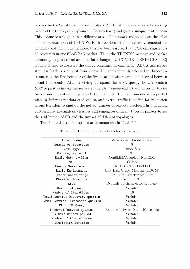
CHAPTER 6. EXPERIMENTAL DESIGN 112
process via the Serial Line Internet Protocol (SLIP). All nodes are placed accordingto one of the topologies (explained in Section 6.3.1) and given 5 unique location tags.This is done to send queries in different areas of a network and to analyse the effectof context-awareness of TRENDY. Each node hosts three resources: temperature,humidity and light. Furthermore, this has been assured that a SA can register itsall resources in one 6LoWPAN packet. Thus, the TRENDY message and packetbecome synonymous and are used interchangeably. CONTIKI’s ENERGEST [33]module is used to measure the energy consumed at each node. All UA queries arestateless (each is sent as if from a new UA) and randomly selected to discover aresource at the DA from one of the five locations after a random interval between0 and 10 seconds. After receiving a response for a SD query, the UA sends aGET request to invoke the service at the SA. Consequently, the number of ServiceInvocation requests are equal to SD queries. All the experiments are repeatedwith 10 different random seed values, and overall traffic is sniffed for validationin one iteration to analyse the actual number of packets produced in a network.Furthermore, the analysis classifies and segregates different types of packets to seethe real burden of SD and the impact of different topologies.
The simulation configurations are summarised in Table 6.2.
Table 6.2: General configurations for experiments
Total nodes Variable + 1 border routerNumber of locations 5
Node Type Tmote SkyRouting protocol RPL
Radio duty cycling ContikiMAC and/or NullRDCMAC CSMA
Energy Measurement ENERGEST (CONTIKI)Radio Environment Unit Disk Graph Medium (UDGM)Transmission range TX: 50m, Interference: 50mPhysical topology Section 6.3.1
Area Depends on the selected topologyNumber of cases Variable
Number of Iterations 10Total Service Discovery queries VariableTotal Service Invocation queries Variable
First UA Query VariableInterval between queries Random between 0 and 10 seconds
DA time window period VariableNumber of time windows Variable
Simulation Duration Variable
CHAPTER 6. EXPERIMENTAL DESIGN 113
6.3.1 Topology
The experiments are done using three different tree topologies. In these topologies,nodes are placed from completely random to a fully controlled way to analyse theeffect of RPL’s generated tree topologies when different TRENDY mechanisms areused. The placement of a node at a certain level of RPL tree is instrumental inits energy consumption. In experiments, each iteration uses a different randomseed value for a COOJA simulation. This value is responsible for the packet order,node start-up time that changes the generation of interrupts. Therefore, the RPLtree construction is also affected by this value and results in a slightly unique treefor each seed values. Following is the description of employed topologies:
Topology#1 - Fully Controlled topology: The RPL topology constructionmechanism (Section 2.3.1) can be controlled by using different RPL’s OFsand ranks for a DODAG. This topology fully exploits this fact and placesthe nodes in different areas while strategically placing only one node in eachgroup one-hop away from the DODAG’s root (where the DA is also placed).However, other nodes in each group are placed randomly, but in a way thatno node from any group is in the radio range of another group’s node. Thewhole topology covers an area of 190m× 180m. The nodes organisation indistant groups is analogous to discussed scenarios in Section 4.2 where nodescan be placed in different building and one resource-rich node that has largetransmission range in each building becomes the parent (in RPL tree) of alllocal nodes. The DODAG’s root (border router) acts as a sink. Figure 6.1ashows the physical topology of 6LoWPAN defined in COOJA simulator.Furthermore, Figure 6.1b presents the RPL tree generated for one COOJAsimulation iteration, which is, in reality, is incongruent to physical topology;however, it matches closely to the physical topology for this topology becauseof its strategic configurations.
Topology#2 - Partially Controlled topology: This topology is similar to to-pology 1, but in each area, nodes are allowed to have overlapping radio accessto nodes in other areas. Therefore, the topology becomes more dense andoccupies an area of 180m× 140m. This topology demonstrates a physicaltopology of nodes in a single building where areas represent different floors.Figure 6.2a shows the physical topology in COOJA and Figure 6.2b presentscorresponding RPL routing topology for one random seed value. In contrastto topology No. 1, it can be noticed that the routing tree is not even for eacharea, and different parent nodes have a different number of branches. This isthe result of RPL parent selection mechanism (described in Section 2.3.1)
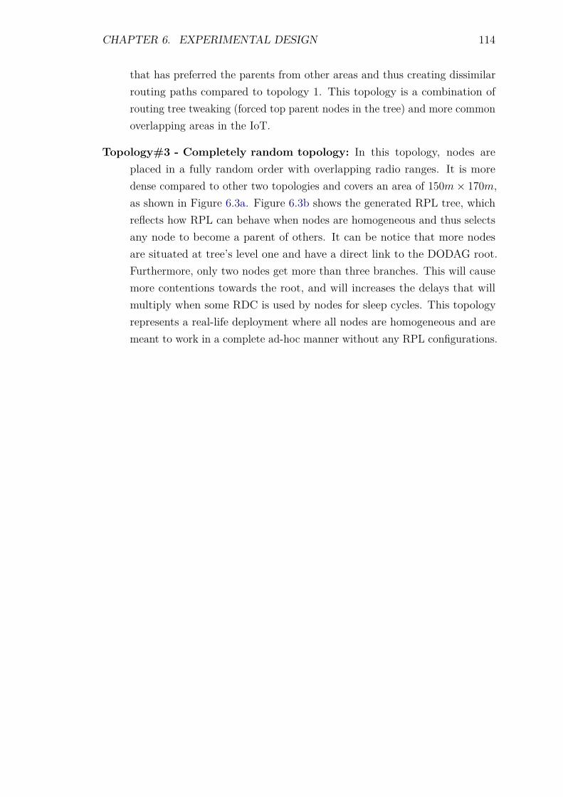
CHAPTER 6. EXPERIMENTAL DESIGN 114
that has preferred the parents from other areas and thus creating dissimilarrouting paths compared to topology 1. This topology is a combination ofrouting tree tweaking (forced top parent nodes in the tree) and more commonoverlapping areas in the IoT.
Topology#3 - Completely random topology: In this topology, nodes areplaced in a fully random order with overlapping radio ranges. It is moredense compared to other two topologies and covers an area of 150m× 170m,as shown in Figure 6.3a. Figure 6.3b shows the generated RPL tree, whichreflects how RPL can behave when nodes are homogeneous and thus selectsany node to become a parent of others. It can be notice that more nodesare situated at tree’s level one and have a direct link to the DODAG root.Furthermore, only two nodes get more than three branches. This will causemore contentions towards the root, and will increases the delays that willmultiply when some RDC is used by nodes for sleep cycles. This topologyrepresents a real-life deployment where all nodes are homogeneous and aremeant to work in a complete ad-hoc manner without any RPL configurations.
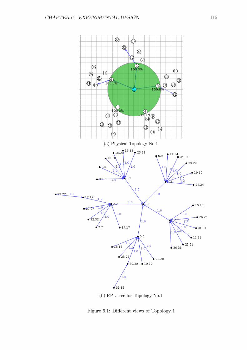
CHAPTER 6. EXPERIMENTAL DESIGN 115
(a) Physical Topology No.1
(b) RPL tree for Topology No.1
Figure 6.1: Different views of Topology 1
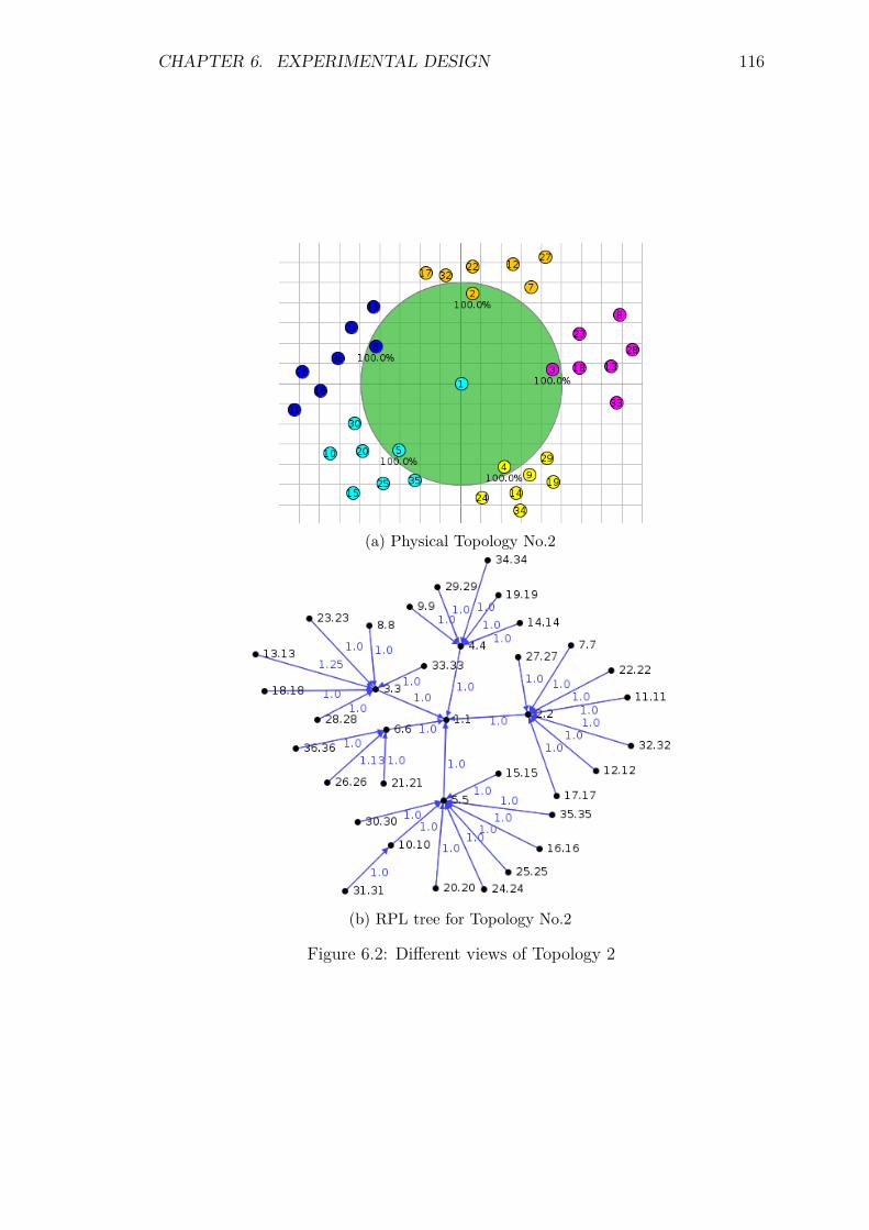
CHAPTER 6. EXPERIMENTAL DESIGN 116
(a) Physical Topology No.2
(b) RPL tree for Topology No.2
Figure 6.2: Different views of Topology 2
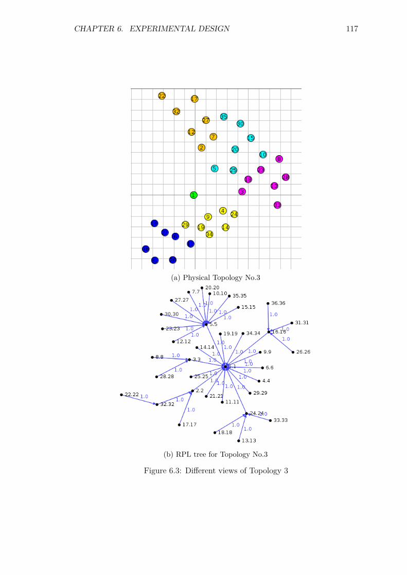
CHAPTER 6. EXPERIMENTAL DESIGN 117
(a) Physical Topology No.3
(b) RPL tree for Topology No.3
Figure 6.3: Different views of Topology 3
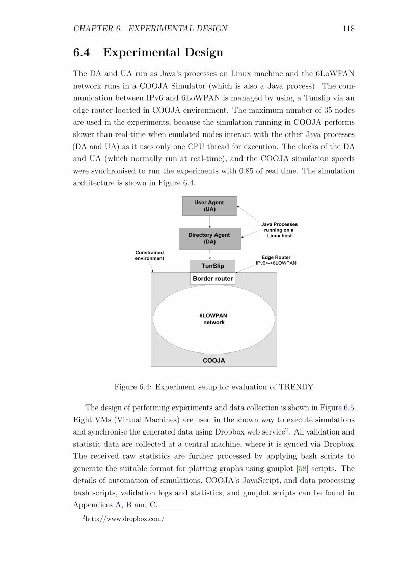
CHAPTER 6. EXPERIMENTAL DESIGN 118
6.4 Experimental Design
The DA and UA run as Java’s processes on Linux machine and the 6LoWPANnetwork runs in a COOJA Simulator (which is also a Java process). The com-munication between IPv6 and 6LoWPAN is managed by using a Tunslip via anedge-router located in COOJA environment. The maximum number of 35 nodesare used in the experiments, because the simulation running in COOJA performsslower than real-time when emulated nodes interact with the other Java processes(DA and UA) as it uses only one CPU thread for execution. The clocks of the DAand UA (which normally run at real-time), and the COOJA simulation speedswere synchronised to run the experiments with 0.85 of real time. The simulationarchitecture is shown in Figure 6.4.
�����
������� ��������
���� ��������
�������������
������ �����
���� �!
�"#" ��������������� �� "
����$ %��
�����"������#����&�� '��� (����
������������
Figure 6.4: Experiment setup for evaluation of TRENDY
The design of performing experiments and data collection is shown in Figure 6.5.Eight VMs (Virtual Machines) are used in the shown way to execute simulationsand synchronise the generated data using Dropbox web service2. All validation andstatistic data are collected at a central machine, where it is synced via Dropbox.The received raw statistics are further processed by applying bash scripts togenerate the suitable format for plotting graphs using gnuplot [58] scripts. Thedetails of automation of simulations, COOJA’s JavaScript, and data processingbash scripts, validation logs and statistics, and gnuplot scripts can be found inAppendices A, B and C.
2http://www.dropbox.com/
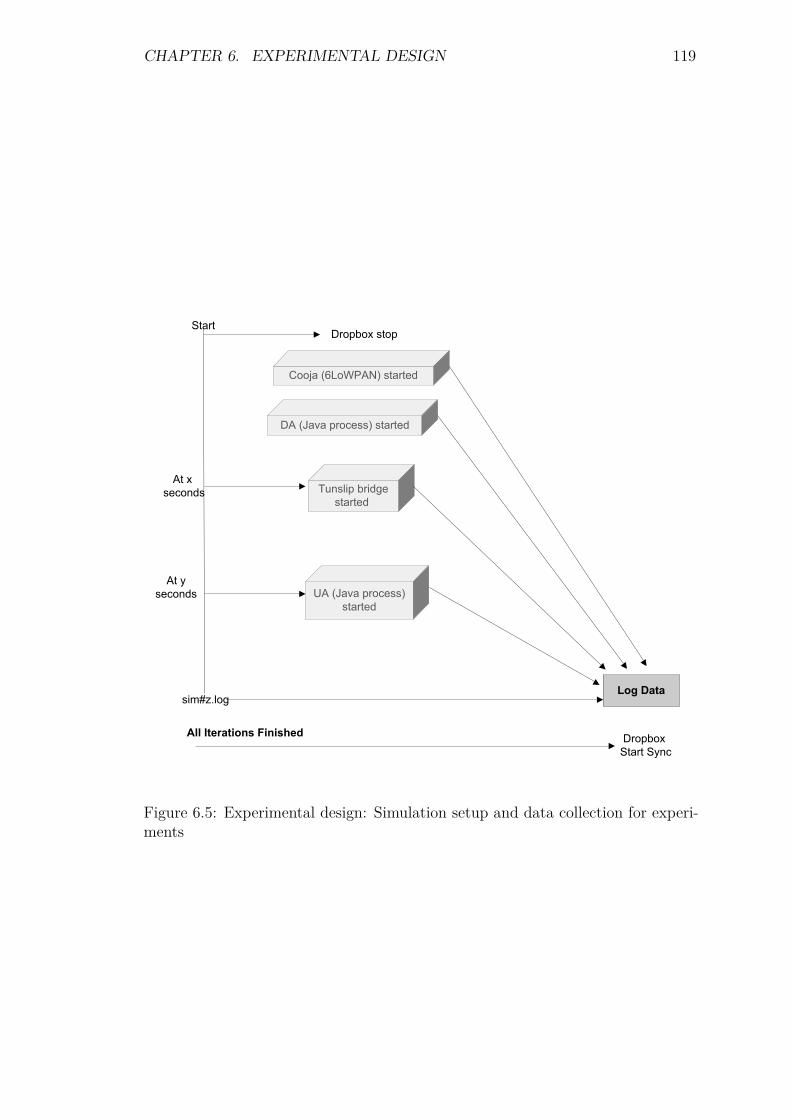
CHAPTER 6. EXPERIMENTAL DESIGN 119
��� �������� ���� ��
����� ������� ������
������� ���
� ����� ����� � ������
��� ��� ������ ������
� � �����
����� ����� � ������
!����
� " �����
�#$%&����� ����
�������!���� !"��
Figure 6.5: Experimental design: Simulation setup and data collection for experi-ments
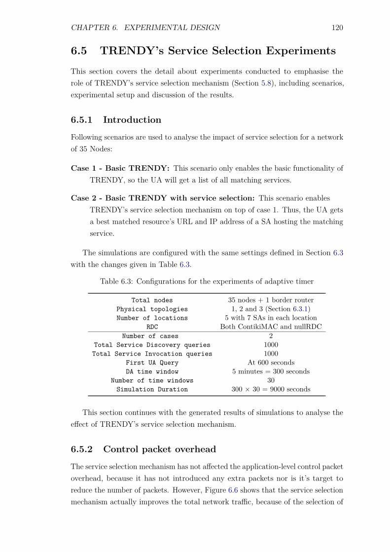
CHAPTER 6. EXPERIMENTAL DESIGN 120
6.5 TRENDY’s Service Selection Experiments
This section covers the detail about experiments conducted to emphasise therole of TRENDY’s service selection mechanism (Section 5.8), including scenarios,experimental setup and discussion of the results.
6.5.1 Introduction
Following scenarios are used to analyse the impact of service selection for a networkof 35 Nodes:
Case 1 - Basic TRENDY: This scenario only enables the basic functionality ofTRENDY, so the UA will get a list of all matching services.
Case 2 - Basic TRENDY with service selection: This scenario enablesTRENDY’s service selection mechanism on top of case 1. Thus, the UA getsa best matched resource’s URL and IP address of a SA hosting the matchingservice.
The simulations are configured with the same settings defined in Section 6.3with the changes given in Table 6.3.
Table 6.3: Configurations for the experiments of adaptive timer
Total nodes 35 nodes + 1 border routerPhysical topologies 1, 2 and 3 (Section 6.3.1)Number of locations 5 with 7 SAs in each location
RDC Both ContikiMAC and nullRDCNumber of cases 2
Total Service Discovery queries 1000Total Service Invocation queries 1000
First UA Query At 600 secondsDA time window 5 minutes = 300 seconds
Number of time windows 30Simulation Duration 300 × 30 = 9000 seconds
This section continues with the generated results of simulations to analyse theeffect of TRENDY’s service selection mechanism.
6.5.2 Control packet overhead
The service selection mechanism has not affected the application-level control packetoverhead, because it has not introduced any extra packets nor is it’s target toreduce the number of packets. However, Figure 6.6 shows that the service selectionmechanism actually improves the total network traffic, because of the selection of
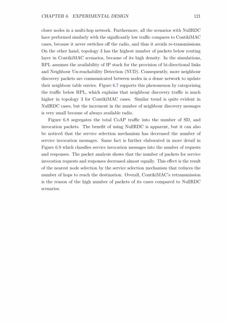
CHAPTER 6. EXPERIMENTAL DESIGN 121
closer nodes in a multi-hop network. Furthermore, all the scenarios with NullRDChave performed similarly with the significantly low traffic compares to ContikiMACcases, because it never switches off the radio, and thus it avoids re-transmissions.On the other hand, topology 3 has the highest number of packets below routinglayer in ContikiMAC scenarios, because of its high density. In the simulations,RPL assumes the availability of IP stack for the provision of bi-directional linksand Neighbour Un-reachability Detection (NUD). Consequently, more neighbourdiscovery packets are communicated between nodes in a dense network to updatetheir neighbour table entries. Figure 6.7 supports this phenomenon by categorisingthe traffic below RPL, which explains that neighbour discovery traffic is muchhigher in topology 3 for ContikiMAC cases. Similar trend is quite evident inNullRDC cases, but the increment in the number of neighbour discovery messagesis very small because of always available radio.
Figure 6.8 segregates the total CoAP traffic into the number of SD, andinvocation packets. The benefit of using NullRDC is apparent, but it can alsobe noticed that the service selection mechanism has decreased the number ofservice invocation messages. Same fact is further elaborated in more detail inFigure 6.9 which classifies service invocation messages into the number of requestsand responses. The packet analysis shows that the number of packets for serviceinvocation requests and responses decreased almost equally. This effect is the resultof the nearest node selection by the service selection mechanism that reduces thenumber of hops to reach the destination. Overall, ContikiMAC’s retransmissionis the reason of the high number of packets of its cases compared to NullRDCscenarios.
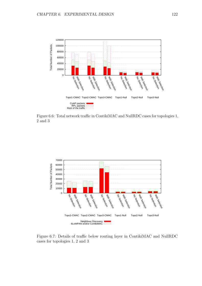
CHAPTER 6. EXPERIMENTAL DESIGN 122
0
20000
40000
60000
80000
100000
120000
No S
electionW
ith Selection
No S
electionW
ith Selection
No S
electionW
ith Selection
No S
electionW
ith Selection
No S
electionW
ith Selection
No S
electionW
ith Selection
Tot
al N
umbe
r of
Pac
kets
CoAP packetsRPL packets
Rest of the traffic
Topo3-NullTopo2-NullTopo1-NullTopo3-CMACTopo2-CMACTopo1-CMAC
Figure 6.6: Total network traffic in ContikiMAC and NullRDC cases for topologies 1,2 and 3
0
10000
20000
30000
40000
50000
60000
70000
No S
electionW
ith Selection
No S
electionW
ith Selection
No S
electionW
ith Selection
No S
electionW
ith Selection
No S
electionW
ith Selection
No S
electionW
ith Selection
Tot
al N
umbe
r of
Pac
kets
Neighbour Discovery6LoWPAN and/or ContikiMAC
Topo3-NullTopo2-NullTopo1-NullTopo3-CMACTopo2-CMACTopo1-CMAC
Figure 6.7: Details of traffic below routing layer in ContikiMAC and NullRDCcases for topologies 1, 2 and 3
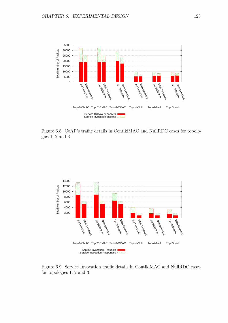
CHAPTER 6. EXPERIMENTAL DESIGN 123
0
5000
10000
15000
20000
25000
30000
35000
No S
electionW
ith Selection
No S
electionW
ith Selection
No S
electionW
ith Selection
No S
electionW
ith Selection
No S
electionW
ith Selection
No S
electionW
ith Selection
Tot
al N
umbe
r of
Pac
kets
Service Discovery packetsService Invocation packets
Topo3-NullTopo2-NullTopo1-NullTopo3-CMACTopo2-CMACTopo1-CMAC
Figure 6.8: CoAP’s traffic details in ContikiMAC and NullRDC cases for topolo-gies 1, 2 and 3
0
2000
4000
6000
8000
10000
12000
14000
No S
electionW
ith Selection
No S
electionW
ith Selection
No S
electionW
ith Selection
No S
electionW
ith Selection
No S
electionW
ith Selection
No S
electionW
ith Selection
Tot
al N
umbe
r of
Pac
kets
Service Invocation RequestsService Invocation Responses
Topo3-NullTopo2-NullTopo1-NullTopo3-CMACTopo2-CMACTopo1-CMAC
Figure 6.9: Service Invocation traffic details in ContikiMAC and NullRDC casesfor topologies 1, 2 and 3
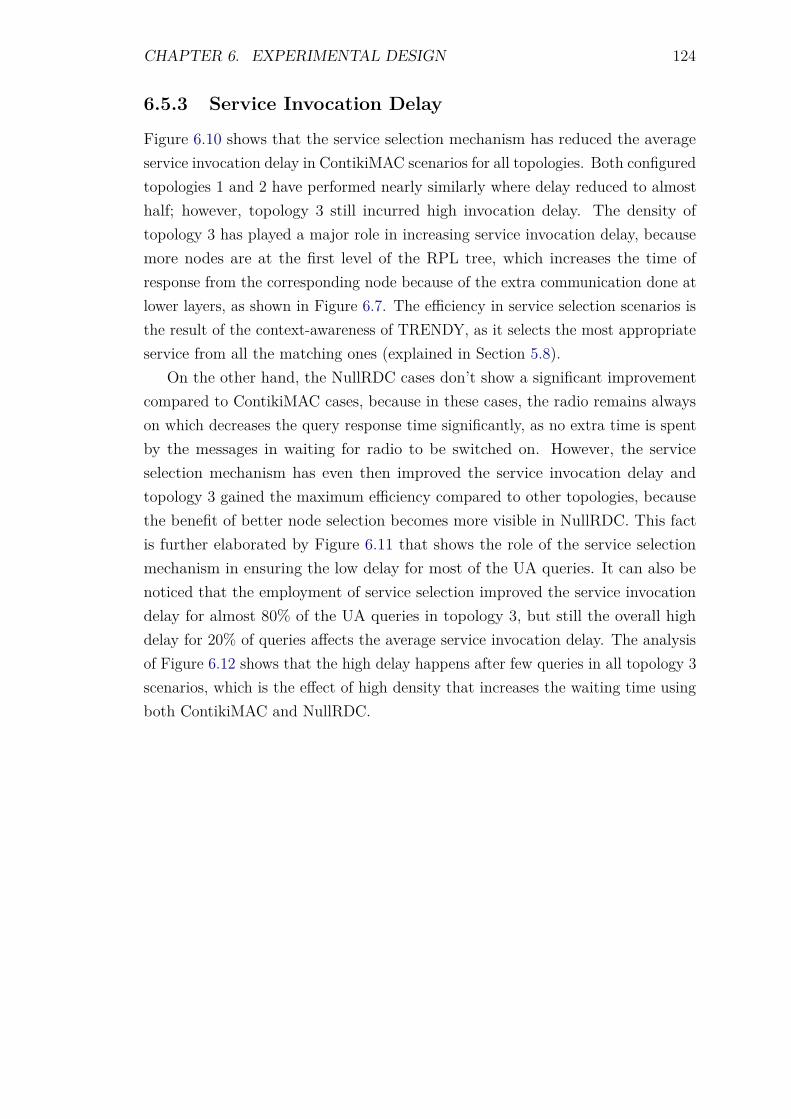
CHAPTER 6. EXPERIMENTAL DESIGN 124
6.5.3 Service Invocation Delay
Figure 6.10 shows that the service selection mechanism has reduced the averageservice invocation delay in ContikiMAC scenarios for all topologies. Both configuredtopologies 1 and 2 have performed nearly similarly where delay reduced to almosthalf; however, topology 3 still incurred high invocation delay. The density oftopology 3 has played a major role in increasing service invocation delay, becausemore nodes are at the first level of the RPL tree, which increases the time ofresponse from the corresponding node because of the extra communication done atlower layers, as shown in Figure 6.7. The efficiency in service selection scenarios isthe result of the context-awareness of TRENDY, as it selects the most appropriateservice from all the matching ones (explained in Section 5.8).
On the other hand, the NullRDC cases don’t show a significant improvementcompared to ContikiMAC cases, because in these cases, the radio remains alwayson which decreases the query response time significantly, as no extra time is spentby the messages in waiting for radio to be switched on. However, the serviceselection mechanism has even then improved the service invocation delay andtopology 3 gained the maximum efficiency compared to other topologies, becausethe benefit of better node selection becomes more visible in NullRDC. This factis further elaborated by Figure 6.11 that shows the role of the service selectionmechanism in ensuring the low delay for most of the UA queries. It can also benoticed that the employment of service selection improved the service invocationdelay for almost 80% of the UA queries in topology 3, but still the overall highdelay for 20% of queries affects the average service invocation delay. The analysisof Figure 6.12 shows that the high delay happens after few queries in all topology 3scenarios, which is the effect of high density that increases the waiting time usingboth ContikiMAC and NullRDC.
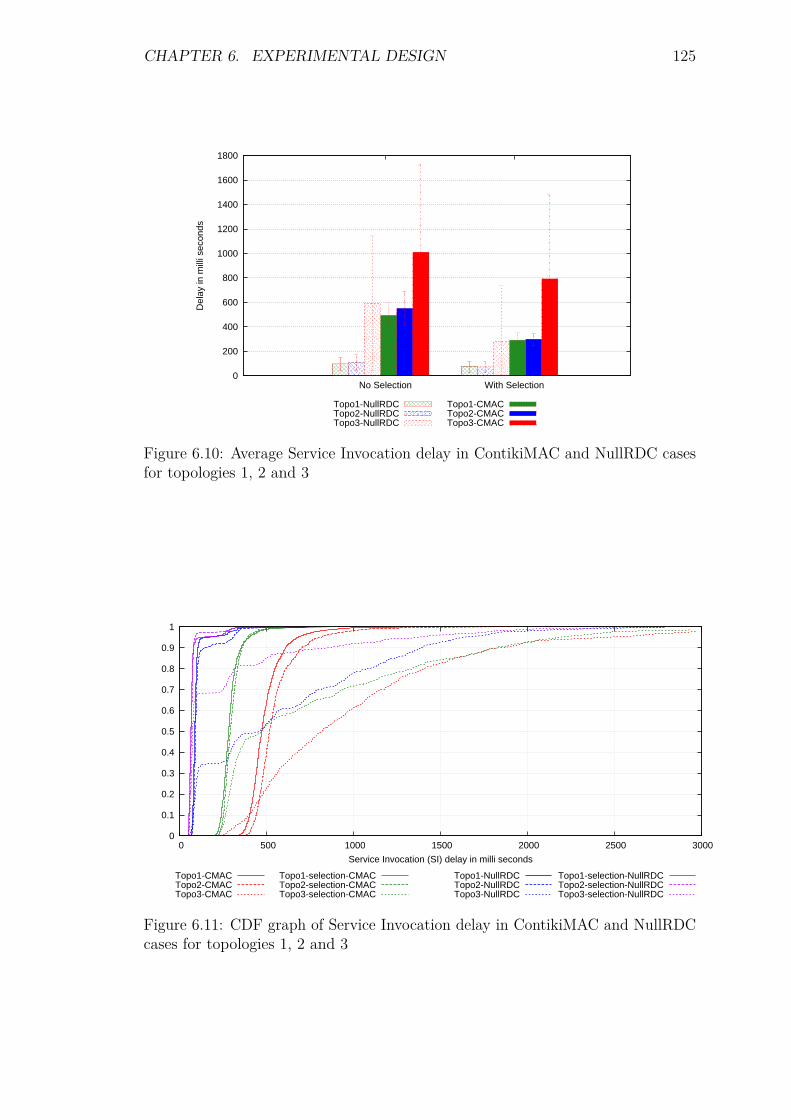
CHAPTER 6. EXPERIMENTAL DESIGN 125
0
200
400
600
800
1000
1200
1400
1600
1800
No Selection With Selection
Del
ay in
mill
i sec
onds
Topo1-NullRDCTopo2-NullRDCTopo3-NullRDC
Topo1-CMACTopo2-CMACTopo3-CMAC
Figure 6.10: Average Service Invocation delay in ContikiMAC and NullRDC casesfor topologies 1, 2 and 3
0
0.1
0.2
0.3
0.4
0.5
0.6
0.7
0.8
0.9
1
0 500 1000 1500 2000 2500 3000
Service Invocation (SI) delay in milli seconds
Topo1-CMACTopo2-CMACTopo3-CMAC
Topo1-selection-CMACTopo2-selection-CMACTopo3-selection-CMAC
Topo1-NullRDCTopo2-NullRDCTopo3-NullRDC
Topo1-selection-NullRDCTopo2-selection-NullRDCTopo3-selection-NullRDC
Figure 6.11: CDF graph of Service Invocation delay in ContikiMAC and NullRDCcases for topologies 1, 2 and 3
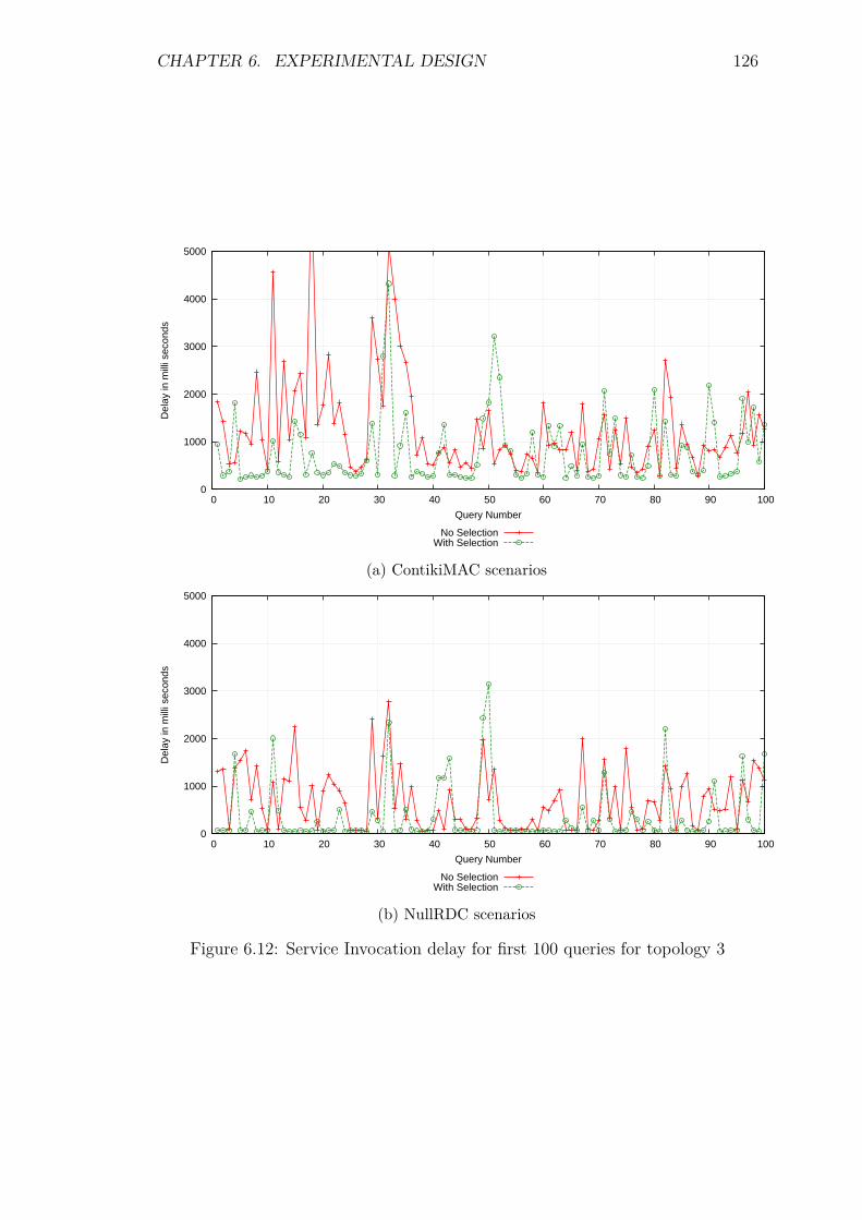
CHAPTER 6. EXPERIMENTAL DESIGN 126
0
1000
2000
3000
4000
5000
0 10 20 30 40 50 60 70 80 90 100
Del
ay in
mill
i sec
onds
Query Number
No SelectionWith Selection
(a) ContikiMAC scenarios
0
1000
2000
3000
4000
5000
0 10 20 30 40 50 60 70 80 90 100
Del
ay in
mill
i sec
onds
Query Number
No SelectionWith Selection
(b) NullRDC scenarios
Figure 6.12: Service Invocation delay for first 100 queries for topology 3
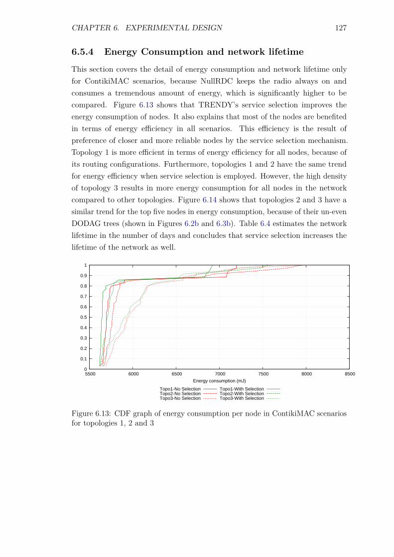
CHAPTER 6. EXPERIMENTAL DESIGN 127
6.5.4 Energy Consumption and network lifetime
This section covers the detail of energy consumption and network lifetime onlyfor ContikiMAC scenarios, because NullRDC keeps the radio always on andconsumes a tremendous amount of energy, which is significantly higher to becompared. Figure 6.13 shows that TRENDY’s service selection improves theenergy consumption of nodes. It also explains that most of the nodes are benefitedin terms of energy efficiency in all scenarios. This efficiency is the result ofpreference of closer and more reliable nodes by the service selection mechanism.Topology 1 is more efficient in terms of energy efficiency for all nodes, because ofits routing configurations. Furthermore, topologies 1 and 2 have the same trendfor energy efficiency when service selection is employed. However, the high densityof topology 3 results in more energy consumption for all nodes in the networkcompared to other topologies. Figure 6.14 shows that topologies 2 and 3 have asimilar trend for the top five nodes in energy consumption, because of their un-evenDODAG trees (shown in Figures 6.2b and 6.3b). Table 6.4 estimates the networklifetime in the number of days and concludes that service selection increases thelifetime of the network as well.
0
0.1
0.2
0.3
0.4
0.5
0.6
0.7
0.8
0.9
1
5500 6000 6500 7000 7500 8000 8500
Energy consumption (mJ)
Topo1-No SelectionTopo2-No SelectionTopo3-No Selection
Topo1-With SelectionTopo2-With SelectionTopo3-With Selection
Figure 6.13: CDF graph of energy consumption per node in ContikiMAC scenariosfor topologies 1, 2 and 3
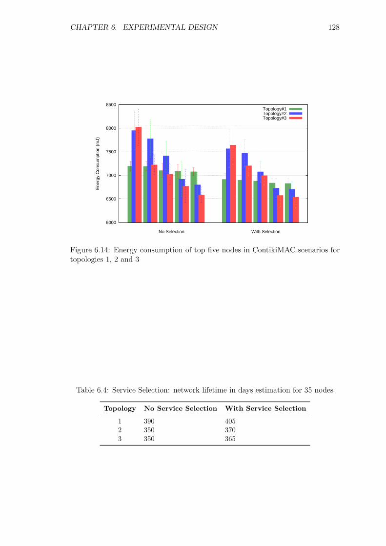
CHAPTER 6. EXPERIMENTAL DESIGN 128
6000
6500
7000
7500
8000
8500
Ene
rgy
Con
sum
ptio
n (m
J)
Topology#1Topology#2Topology#3
With SelectionNo Selection
Figure 6.14: Energy consumption of top five nodes in ContikiMAC scenarios fortopologies 1, 2 and 3
Table 6.4: Service Selection: network lifetime in days estimation for 35 nodes
Topology No Service Selection With Service Selection
1 390 4052 350 3703 350 365

CHAPTER 6. EXPERIMENTAL DESIGN 129
6.5.5 Packets at the DA: a scalability factor
TRENDY’s service selection is not aimed to decrease the number of packets at theDA, so all cases have the similar number of application-level messages receivedat the DA (excluding service invocation messages). However, Figure 6.15 showsthat there is a slight benefit of using the service selection mechanism in topology 3in terms of total traffic to or from the DA. This gain comes from the reductionof the number of neighbour discovery messages, because the DA sits on tops ofDODAG’s root and once the closest node is selected to serve a query its entryin the neighbour’s table (maintained by neighbour discovery) is also updated.Consequently, the network traffic in topology 3 that’s decreased around 10%.
0
10000
20000
30000
40000
50000
60000
No Selection With Selection
Num
ber
of P
acke
ts
Topo1-NullRDCTopo2-NullRDCTopo3-NullRDC
Topo1-CMACTopo2-CMACTopo3-CMAC
Figure 6.15: The DA traffic in ContikiMAC and NullRDC cases for topologies 1, 2and 3
6.5.6 Reliability and Accuracy
The reliability and accuracy of TRENDY are explained in Section 6.2.6 holds truefor service selection scenarios. However, the context-aware selection of service hostsincreases the reliability, because the selection criteria (Section 5.8) chooses themost reliable SA. All service invocation responses are verified and validated, usinglogs and sniffed packets (Appendix B), and are found accurate. Consequently, it isconcluded from the validation that the DA has always sent reliable SD informationto the DA.
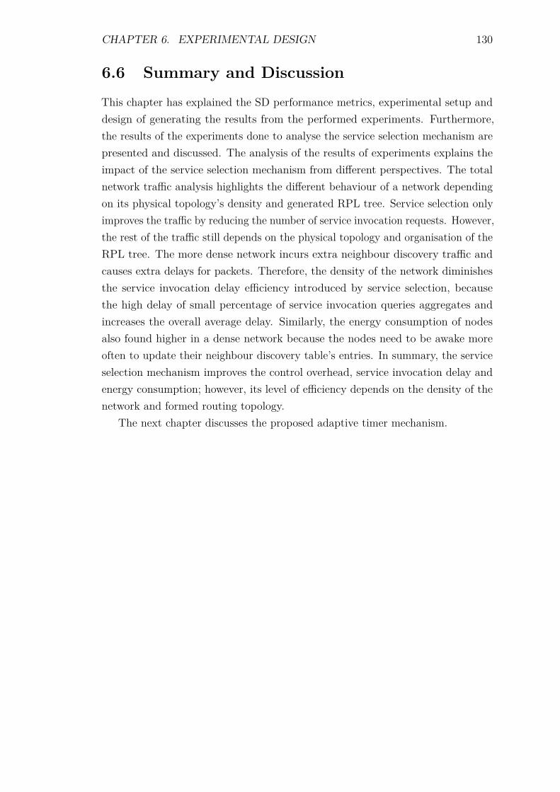
CHAPTER 6. EXPERIMENTAL DESIGN 130
6.6 Summary and Discussion
This chapter has explained the SD performance metrics, experimental setup anddesign of generating the results from the performed experiments. Furthermore,the results of the experiments done to analyse the service selection mechanism arepresented and discussed. The analysis of the results of experiments explains theimpact of the service selection mechanism from different perspectives. The totalnetwork traffic analysis highlights the different behaviour of a network dependingon its physical topology’s density and generated RPL tree. Service selection onlyimproves the traffic by reducing the number of service invocation requests. However,the rest of the traffic still depends on the physical topology and organisation of theRPL tree. The more dense network incurs extra neighbour discovery traffic andcauses extra delays for packets. Therefore, the density of the network diminishesthe service invocation delay efficiency introduced by service selection, becausethe high delay of small percentage of service invocation queries aggregates andincreases the overall average delay. Similarly, the energy consumption of nodesalso found higher in a dense network because the nodes need to be awake moreoften to update their neighbour discovery table’s entries. In summary, the serviceselection mechanism improves the control overhead, service invocation delay andenergy consumption; however, its level of efficiency depends on the density of thenetwork and formed routing topology.
The next chapter discusses the proposed adaptive timer mechanism.
Chapter 7
Adaptive Reporting Timer
7.1 Introduction
Chapter 5 proposes a context-aware SD solution for the IoT. The solution providesan interoperable and open framework to work with different data formats accessibleusing compact CoAP-based RESTful web services. However, all services areregistered at the DA and then status maintenance messages required to be sent tothe DA as well. The generated traffic increases the energy consumption of nodes, asother nodes usually need to pass the control traffic towards the DA in a multi-hopnetwork. This chapter proposes an adaptive timer algorithm that reduces thecontrol traffic. Consequently, nodes become energy efficient and scalability is alsoimproved, as control traffic not remains linearly proportional to the increasingnumber of nodes in a network. The detail of the mechanism’s aims and challenges,design, message format and experiments with the results are covered in this chapter.
7.2 Aims
The main goal of the adaptive timer algorithm is to decrease the number of controlpackets by adaptively increasing the interval between status updates. This hasmultiple benefits: it will decrease the control packet overhead and will improvethe energy consumption. However, this will consequently, sacrifice the inherentreliability by increasing the probability that the DA will forward stale (outdated)information to a UA. Therefore, the challenge for timer is to reduce this risk bysensing the requirements of a network and its dynamics.
Following is the summary of the timer mechanism’s objectives:
1. The number of status updates should be reduced to improve the energyconsumption of constrained nodes and network.
131
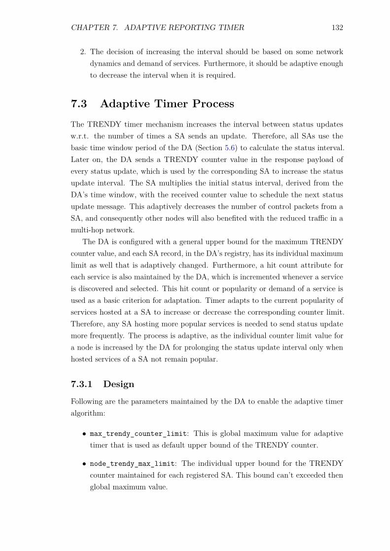
CHAPTER 7. ADAPTIVE REPORTING TIMER 132
2. The decision of increasing the interval should be based on some networkdynamics and demand of services. Furthermore, it should be adaptive enoughto decrease the interval when it is required.
7.3 Adaptive Timer Process
The TRENDY timer mechanism increases the interval between status updatesw.r.t. the number of times a SA sends an update. Therefore, all SAs use thebasic time window period of the DA (Section 5.6) to calculate the status interval.Later on, the DA sends a TRENDY counter value in the response payload ofevery status update, which is used by the corresponding SA to increase the statusupdate interval. The SA multiplies the initial status interval, derived from theDA’s time window, with the received counter value to schedule the next statusupdate message. This adaptively decreases the number of control packets from aSA, and consequently other nodes will also benefited with the reduced traffic in amulti-hop network.
The DA is configured with a general upper bound for the maximum TRENDYcounter value, and each SA record, in the DA’s registry, has its individual maximumlimit as well that is adaptively changed. Furthermore, a hit count attribute foreach service is also maintained by the DA, which is incremented whenever a serviceis discovered and selected. This hit count or popularity or demand of a service isused as a basic criterion for adaptation. Timer adapts to the current popularity ofservices hosted at a SA to increase or decrease the corresponding counter limit.Therefore, any SA hosting more popular services is needed to send status updatemore frequently. The process is adaptive, as the individual counter limit value fora node is increased by the DA for prolonging the status update interval only whenhosted services of a SA not remain popular.
7.3.1 Design
Following are the parameters maintained by the DA to enable the adaptive timeralgorithm:
• max_trendy_counter_limit: This is global maximum value for adaptivetimer that is used as default upper bound of the TRENDY counter.
• node_trendy_max_limit: The individual upper bound for the TRENDYcounter maintained for each registered SA. This bound can’t exceeded thenglobal maximum value.

CHAPTER 7. ADAPTIVE REPORTING TIMER 133
• hit_count_threshold: The threshold value to determine the decision pointwhen hosted services of a SA become enough popular. This attribute is usedby the DA before increasing or decreasing node_trendy_max_limit of a SA.This threshold can be set at any value up to the application requirements, andits effect will only become apparent when same service is selected multipletimes for SD queries.
• retain_threshold: It determines the mimimum number of hit counts re-quired to keep the decremented node_trendy_max_limit unchanged.
• timer_step: Whenever the hit_count_threshold is exceeded, thenode_trendy_max_limit is decremented by this value for the correspondingSA. This step value is also used to increment the SA’s maximum limit whenhit count remains less than retain_threshold.
• node_trendy_counter: It represents the TRENDY counter value for eachregistered SA, and its value never surpasses node_trendy_max_limit.
• node_trendy_current: This attribute is updated with node_trendy_countervalue each time a status update is received from a SA. This value is decre-mented after every time window until reaches to 1.
• node_trendy_counter_changed: This is a flag used to ensure that multiplechanges are not made to a node_trendy_counter in one time window.
All attributes starting with node prefix are maintained for each SA, whereasothers have global scope. Each SA only requires trendy_counter attribute thathas a default value set at 1, which is updated when a new value is received fromthe DA
Following is the procedure of the adaptive timer:
Step 1 - Initiation: The DA starts with the configured parameters, and it followsthe Algorithm 1 when it receives a registration message from a SA. Thisalgorithm initialises the TRENDY counter variables for the node and setsthe flag to avoid multiple changes in its value with in a time window. TheSA gets a basic time window period in response to its successful registrationat the DA.
Step 2 - Evaluation on receiving a Status update message: The DA followsAlgorithm 2 at receipt of every status update message. This algorithm checksand increment the node_trendy_counter, which subsequently enables theSA to increase the time period for its next status update message. This
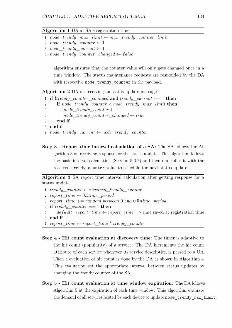
CHAPTER 7. ADAPTIVE REPORTING TIMER 134
Algorithm 1 DA at SA’s registration time1: node_trendy_max_limit← max_trendy_counter_limit2: node_trendy_counter ← 13: node_trendy_current← 14: node_trendy_counter_changed← false
algorithm ensures that the counter value will only gets changed once in atime window. The status maintenance requests are responded by the DAwith respective node_trendy_counter in the payload.
Algorithm 2 DA on receiving an status update message1: if !trendy_counter_changed and trendy_current == 1 then2: if node_trendy_counter < node_trendy_max_limit then3: node_trendy_counter + +4: node_trendy_counter_changed← true5: end if6: end if7: node_trendy_current← node_trendy_counter
Step 3 - Report time interval calculation of a SA: The SA follows the Al-gorithm 3 on receiving response for the status update. This algorithm followsthe basic interval calculation (Section 5.6.2) and then multiplies it with thereceived trendy_counter value to schedule the next status update.
Algorithm 3 SA report time interval calculation after getting response for astatus update1: trendy_counter ← received_trendy_counter2: report_time← 0.5time_period3: report_time += random(between 0 and 0.5)time_period4: if trendy_counter == 1 then5: default_report_time← report_time . time saved at registration time6: end if7: report_time← report_time * trendy_counter
Step 4 - Hit count evaluation at discovery time: The timer is adaptive tothe hit count (popularity) of a service. The DA increments the hit countattribute of each service whenever its service description is passed to a UA.Then a evaluation of hit count is done by the DA as shown in Algorithm 4.This evaluation set the appropriate interval between status updates bychanging the trendy counter of the SA.
Step 5 - Hit count evaluation at time window expiration: The DA followsAlgorithm 5 at the expiration of each time window. This algorithm evaluatethe demand of all services hosted by each device to update node_trendy_max_limit.

CHAPTER 7. ADAPTIVE REPORTING TIMER 135
Algorithm 4 Hit count evaluation at discovery time1: if node_hit_count > hit_count_threshold then2: node_trendy_max_limit← node_trendy_max_limit− timer_step3: trendy_counter_changed← true4: node_hit_count← 05: end if
Algorithm 5 Hit count evaluation at end of a time window1: if trendy_counter_changed == false then2: if hit_count < retain_threshold then3: node_trendy_max_limit← node_trendy_max_limit + timer_step4: trendy_counter_changed← true5: if node_trendy_max_limit > max_trendy_counter_limit then6: node_trendy_max_limit← max_trendy_counter_limit7: end if8: end if9: end if
7.3.2 Example Scenario
This section demonstrates the working of the timer mechanism by explaining itwith some scenarios expressed in figures, which depict adaptive timer mechanismin action at different stages.
Figure 7.1 describes the adaptive timer in a scenario, where the hit countthreshold was set at 2. The counter value kept on increasing over the time andreached its maximum. It keeps on updating the DA with the same large intervaluntil its services become popular. The algorithm assesses this change of demand,and adaptively changes the maximum counter limit value to reduce the statusupdate interval for the particular SA. Furthermore, Figure 7.2 shows the samescenario in the long run and describes the behaviour of timer when a service is notin demand for a SA. Moreover, Figure 7.3 expresses a possible state of the networkwhile using the adaptive timer mechanism, where the nodes have different intervalsas a result of the diversity of SD queries.

CHAPTER 7. ADAPTIVE REPORTING TIMER 136
�
��� �������� ��
�� � ����� ���� ��� ���� ��
����
�����
�����
������
������
����
����
����� !�"$� %��%�&� ' ����� ��� ' �
���� %��%�&� ' ������( ' �
�������
�����������
���
��� �� ' ������( ' )
�����
�����
Figure 7.1: Adaptive timer’s in a scenario
��������
�� �� �� �� �� �� �� �� �� �� �� �� ��
��
����������
�� ��
��
�� ����
�� ��
��
�� ��
���
��
�� ����
�� ��
���
���� ��
����������
�� � ���� ��� ��
Figure 7.2: Timer’s adaptability in the long run
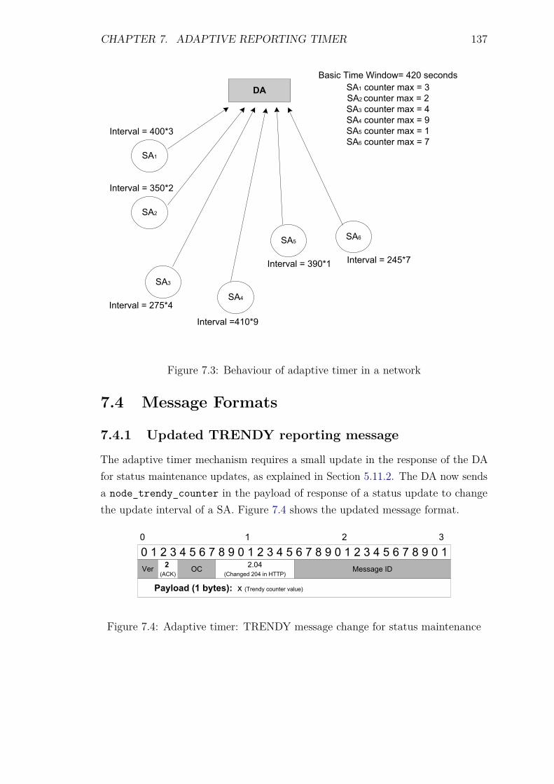
CHAPTER 7. ADAPTIVE REPORTING TIMER 137
��
���
����� �� �� ���� ��� ���� ��
� ������ � �����
���
� ������ � �����
���
� ������ � ��������
� ������ ������
���
� ������ � �����
���
� ������ � �����
��� �� ��� �! � ���� �� ��� �! � ���� �� ��� �! � ���� �� ��� �! � ���� �� ��� �! � ���� �� ��� �! � �
Figure 7.3: Behaviour of adaptive timer in a network
7.4 Message Formats
7.4.1 Updated TRENDY reporting message
The adaptive timer mechanism requires a small update in the response of the DAfor status maintenance updates, as explained in Section 5.11.2. The DA now sendsa node_trendy_counter in the payload of response of a status update to changethe update interval of a SA. Figure 7.4 shows the updated message format.
� � � � � � � � � � � � � � � � � � � � � � � � � ��� ��
������� �� ��� � � �� ���� ������ ������
� � � �
���� �
�!����#��$�� ��� %� &��'�
(�))�$� *+
Figure 7.4: Adaptive timer: TRENDY message change for status maintenance
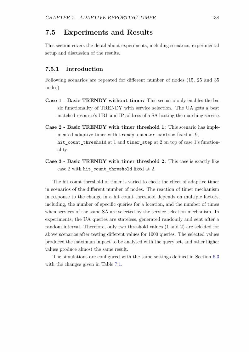
CHAPTER 7. ADAPTIVE REPORTING TIMER 138
7.5 Experiments and Results
This section covers the detail about experiments, including scenarios, experimentalsetup and discussion of the results.
7.5.1 Introduction
Following scenarios are repeated for different number of nodes (15, 25 and 35nodes).
Case 1 - Basic TRENDY without timer: This scenario only enables the ba-sic functionality of TRENDY with service selection. The UA gets a bestmatched resource’s URL and IP address of a SA hosting the matching service.
Case 2 - Basic TRENDY with timer threshold 1: This scenario has imple-mented adaptive timer with trendy_counter_maximum fixed at 9,hit_count_threshold at 1 and timer_step at 2 on top of case 1’s function-ality.
Case 3 - Basic TRENDY with timer threshold 2: This case is exactly likecase 2 with hit_count_threshold fixed at 2.
The hit count threshold of timer is varied to check the effect of adaptive timerin scenarios of the different number of nodes. The reaction of timer mechanismin response to the change in a hit count threshold depends on multiple factors,including, the number of specific queries for a location, and the number of timeswhen services of the same SA are selected by the service selection mechanism. Inexperiments, the UA queries are stateless, generated randomly and sent after arandom interval. Therefore, only two threshold values (1 and 2) are selected forabove scenarios after testing different values for 1000 queries. The selected valuesproduced the maximum impact to be analysed with the query set, and other highervalues produce almost the same result.
The simulations are configured with the same settings defined in Section 6.3with the changes given in Table 7.1.
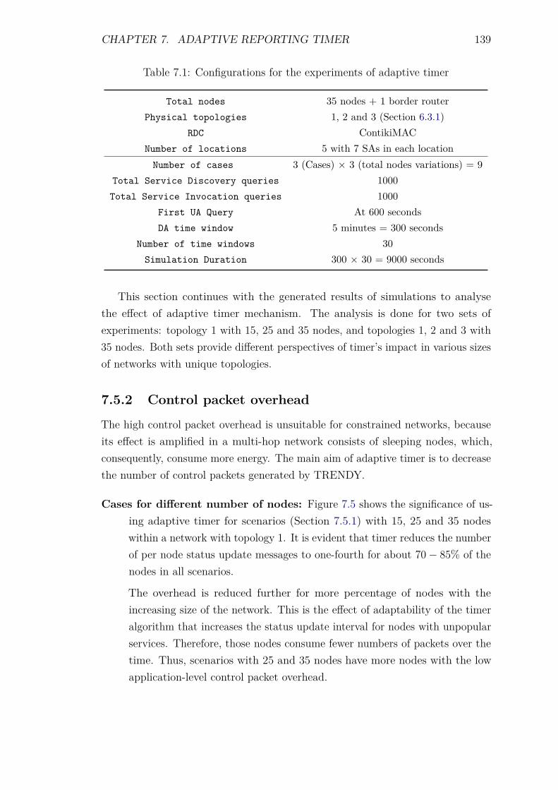
CHAPTER 7. ADAPTIVE REPORTING TIMER 139
Table 7.1: Configurations for the experiments of adaptive timer
Total nodes 35 nodes + 1 border routerPhysical topologies 1, 2 and 3 (Section 6.3.1)
RDC ContikiMACNumber of locations 5 with 7 SAs in each location
Number of cases 3 (Cases) × 3 (total nodes variations) = 9Total Service Discovery queries 1000Total Service Invocation queries 1000
First UA Query At 600 secondsDA time window 5 minutes = 300 seconds
Number of time windows 30Simulation Duration 300 × 30 = 9000 seconds
This section continues with the generated results of simulations to analysethe effect of adaptive timer mechanism. The analysis is done for two sets ofexperiments: topology 1 with 15, 25 and 35 nodes, and topologies 1, 2 and 3 with35 nodes. Both sets provide different perspectives of timer’s impact in various sizesof networks with unique topologies.
7.5.2 Control packet overhead
The high control packet overhead is unsuitable for constrained networks, becauseits effect is amplified in a multi-hop network consists of sleeping nodes, which,consequently, consume more energy. The main aim of adaptive timer is to decreasethe number of control packets generated by TRENDY.
Cases for different number of nodes: Figure 7.5 shows the significance of us-ing adaptive timer for scenarios (Section 7.5.1) with 15, 25 and 35 nodeswithin a network with topology 1. It is evident that timer reduces the numberof per node status update messages to one-fourth for about 70− 85% of thenodes in all scenarios.
The overhead is reduced further for more percentage of nodes with theincreasing size of the network. This is the effect of adaptability of the timeralgorithm that increases the status update interval for nodes with unpopularservices. Therefore, those nodes consume fewer numbers of packets over thetime. Thus, scenarios with 25 and 35 nodes have more nodes with the lowapplication-level control packet overhead.

CHAPTER 7. ADAPTIVE REPORTING TIMER 140
0
0.1
0.2
0.3
0.4
0.5
0.6
0.7
0.8
0.9
1
5 10 15 20 25 30 35 40 45
Number of packets
15 Nodes-No Timer25 Nodes-No Timer35 Nodes-No Timer
15 Nodes-Timer (t=1)25 Nodes-Timer (t=1)35 Nodes-Timer (t=1)
15 Nodes-Timer (t=2)25 Nodes-Timer (t=2)35 Nodes-Timer (t=2)
Figure 7.5: CDF graph of application-level control packet overhead per node withdifferent timer threshold values for topology 1
Figure 7.6 shows the aggregated control overhead for all nodes in the network.It is clearly evident in the figure that employment of adaptive timer makesthe solution scalable as increasing number of nodes only marginally increasesthe control overhead. The scenarios with 35 nodes have performed the best,where the number of packets reduced to more than one-third with the usageof adaptive timer because of the aggregated benefit of all nodes. In addition,Figure 7.7 shows the same trend in terms of total network traffic overhead.It can also be noticed that the decreased number of CoAP packets has alsoreduced the number of packets at layers below RPL in all scenarios. Moreover,Figure 7.8 presents the detail of CoAP packets by categorising those in SDand invocation packets. The number of SD packets in scenarios with timerdemonstrate the same scalable behaviour. The cases with the hit countthreshold 1 and 2 performed almost similarly because of the randomness ofthe used query set and the effect of service selection that chooses a betterSA each time and hence reduced the number of hit counts for services. Insummary, the rate of control packet overhead is not proportional to theincreasing number of nodes, which indicates that timer has made the solutionscalable.
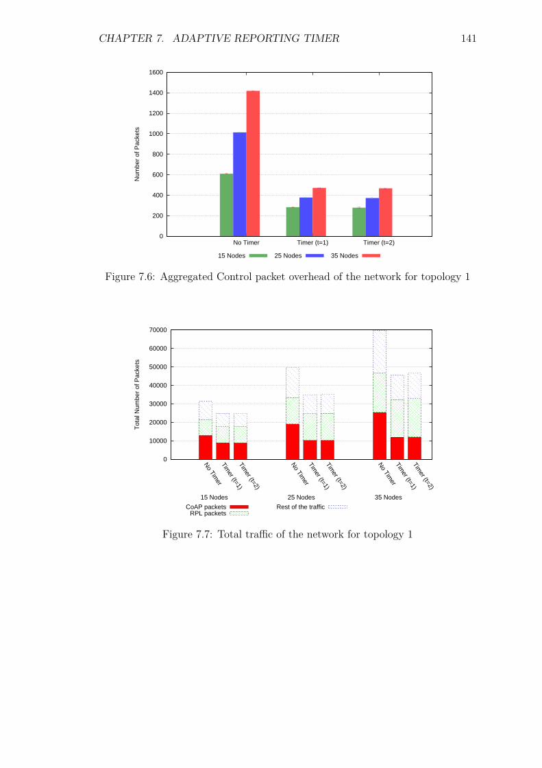
CHAPTER 7. ADAPTIVE REPORTING TIMER 141
0
200
400
600
800
1000
1200
1400
1600
No Timer Timer (t=1) Timer (t=2)
Num
ber
of P
acke
ts
15 Nodes 25 Nodes 35 Nodes
Figure 7.6: Aggregated Control packet overhead of the network for topology 1
0
10000
20000
30000
40000
50000
60000
70000N
o Timer
Timer (t=1)
Timer (t=2)
No Tim
erTim
er (t=1)Tim
er (t=2)
No Tim
erTim
er (t=1)Tim
er (t=2)
Tot
al N
umbe
r of
Pac
kets
CoAP packetsRPL packets
Rest of the traffic
35 Nodes25 Nodes15 Nodes
Figure 7.7: Total traffic of the network for topology 1
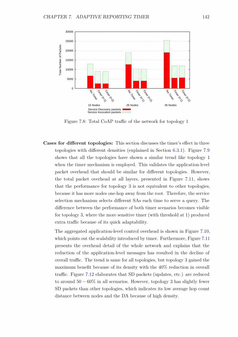
CHAPTER 7. ADAPTIVE REPORTING TIMER 142
0
5000
10000
15000
20000
25000
30000
No Tim
erTim
er (t=1)Tim
er (t=2)
No Tim
erTim
er (t=1)Tim
er (t=2)
No Tim
erTim
er (t=1)Tim
er (t=2)
Tot
al N
umbe
r of
Pac
kets
Service Discovery packetsService Invocation packets
35 Nodes25 Nodes15 Nodes
Figure 7.8: Total CoAP traffic of the network for topology 1
Cases for different topologies: This section discusses the timer’s effect in threetopologies with different densities (explained in Section 6.3.1). Figure 7.9shows that all the topologies have shown a similar trend like topology 1when the timer mechanism is employed. This validates the application-levelpacket overhead that should be similar for different topologies. However,the total packet overhead at all layers, presented in Figure 7.11, showsthat the performance for topology 3 is not equivalent to other topologies,because it has more nodes one-hop away from the root. Therefore, the serviceselection mechanism selects different SAs each time to serve a query. Thedifference between the performance of both timer scenarios becomes visiblefor topology 3, where the more sensitive timer (with threshold at 1) producedextra traffic because of its quick adaptability.
The aggregated application-level control overhead is shown in Figure 7.10,which points out the scalability introduced by timer. Furthermore, Figure 7.11presents the overhead detail of the whole network and explains that thereduction of the application-level messages has resulted in the decline ofoverall traffic. The trend is same for all topologies, but topology 3 gained themaximum benefit because of its density with the 40% reduction in overalltraffic. Figure 7.12 elaborates that SD packets (updates, etc.) are reducedto around 50− 60% in all scenarios. However, topology 3 has slightly fewerSD packets than other topologies, which indicates its low average hop countdistance between nodes and the DA because of high density.
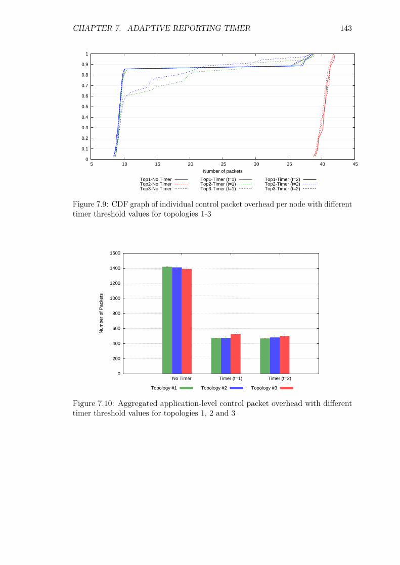
CHAPTER 7. ADAPTIVE REPORTING TIMER 143
0
0.1
0.2
0.3
0.4
0.5
0.6
0.7
0.8
0.9
1
5 10 15 20 25 30 35 40 45
Number of packets
Top1-No TimerTop2-No TimerTop3-No Timer
Top1-Timer (t=1)Top2-Timer (t=1)Top3-Timer (t=1)
Top1-Timer (t=2)Top2-Timer (t=2)Top3-Timer (t=2)
Figure 7.9: CDF graph of individual control packet overhead per node with differenttimer threshold values for topologies 1-3
0
200
400
600
800
1000
1200
1400
1600
No Timer Timer (t=1) Timer (t=2)
Num
ber
of P
acke
ts
Topology #1 Topology #2 Topology #3
Figure 7.10: Aggregated application-level control packet overhead with differenttimer threshold values for topologies 1, 2 and 3
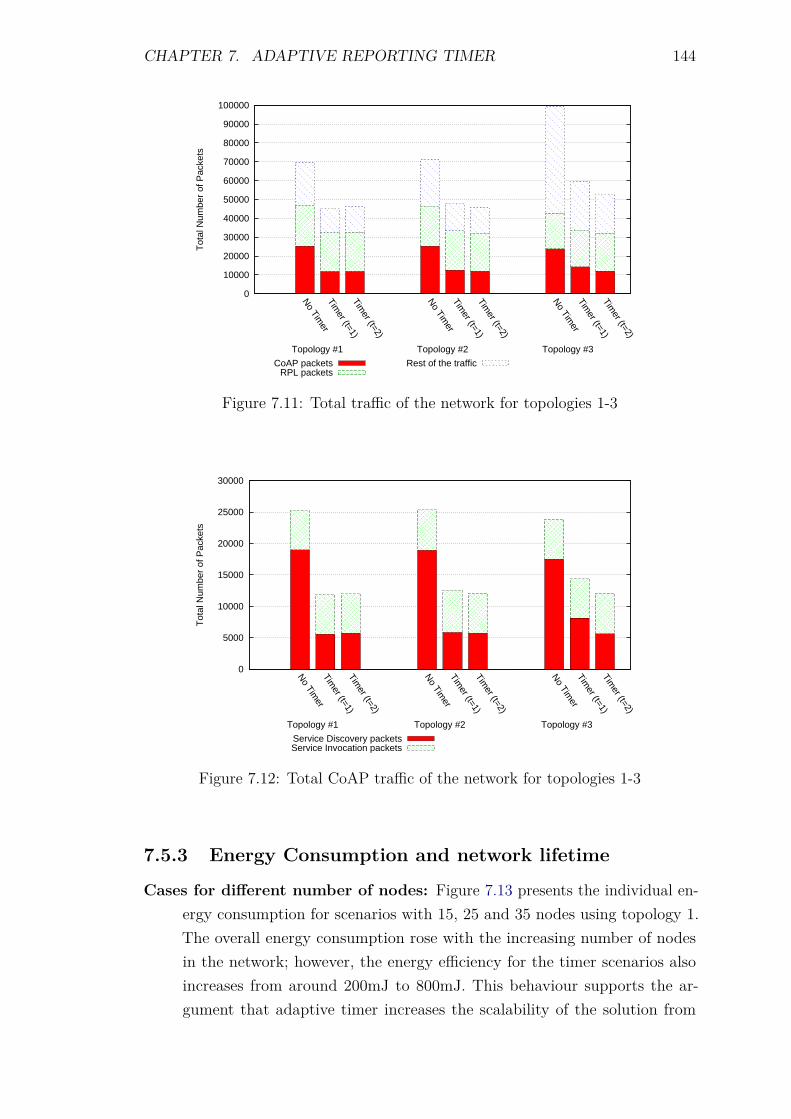
CHAPTER 7. ADAPTIVE REPORTING TIMER 144
0
10000
20000
30000
40000
50000
60000
70000
80000
90000
100000
No Tim
erTim
er (t=1)Tim
er (t=2)
No Tim
erTim
er (t=1)Tim
er (t=2)
No Tim
erTim
er (t=1)Tim
er (t=2)
Tot
al N
umbe
r of
Pac
kets
CoAP packetsRPL packets
Rest of the traffic
Topology #3Topology #2Topology #1
Figure 7.11: Total traffic of the network for topologies 1-3
0
5000
10000
15000
20000
25000
30000N
o Timer
Timer (t=1)
Timer (t=2)
No Tim
erTim
er (t=1)Tim
er (t=2)
No Tim
erTim
er (t=1)Tim
er (t=2)
Tot
al N
umbe
r of
Pac
kets
Service Discovery packetsService Invocation packets
Topology #3Topology #2Topology #1
Figure 7.12: Total CoAP traffic of the network for topologies 1-3
7.5.3 Energy Consumption and network lifetime
Cases for different number of nodes: Figure 7.13 presents the individual en-ergy consumption for scenarios with 15, 25 and 35 nodes using topology 1.The overall energy consumption rose with the increasing number of nodesin the network; however, the energy efficiency for the timer scenarios alsoincreases from around 200mJ to 800mJ. This behaviour supports the ar-gument that adaptive timer increases the scalability of the solution from
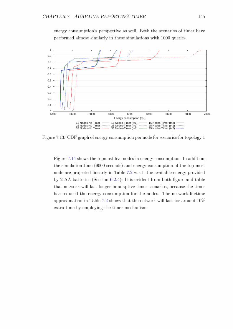
CHAPTER 7. ADAPTIVE REPORTING TIMER 145
energy consumption’s perspective as well. Both the scenarios of timer haveperformed almost similarly in these simulations with 1000 queries.
0
0.1
0.2
0.3
0.4
0.5
0.6
0.7
0.8
0.9
1
5400 5600 5800 6000 6200 6400 6600 6800 7000
Energy consumption (mJ)
15 Nodes-No Timer25 Nodes-No Timer35 Nodes-No Timer
15 Nodes-Timer (t=1)25 Nodes-Timer (t=1)35 Nodes-Timer (t=1)
15 Nodes-Timer (t=2)25 Nodes-Timer (t=2)35 Nodes-Timer (t=2)
Figure 7.13: CDF graph of energy consumption per node for scenarios for topology 1
Figure 7.14 shows the topmost five nodes in energy consumption. In addition,the simulation time (9000 seconds) and energy consumption of the top-mostnode are projected linearly in Table 7.2 w.r.t. the available energy providedby 2 AA batteries (Section 6.2.4). It is evident from both figure and tablethat network will last longer in adaptive timer scenarios, because the timerhas reduced the energy consumption for the nodes. The network lifetimeapproximation in Table 7.2 shows that the network will last for around 10%extra time by employing the timer mechanism.
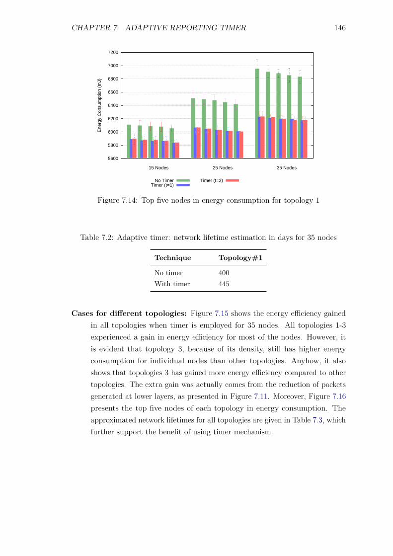
CHAPTER 7. ADAPTIVE REPORTING TIMER 146
5600
5800
6000
6200
6400
6600
6800
7000
7200
Ene
rgy
Con
sum
ptio
n (m
J)
No TimerTimer (t=1)
Timer (t=2)
35 Nodes25 Nodes15 Nodes
Figure 7.14: Top five nodes in energy consumption for topology 1
Table 7.2: Adaptive timer: network lifetime estimation in days for 35 nodes
Technique Topology#1
No timer 400With timer 445
Cases for different topologies: Figure 7.15 shows the energy efficiency gainedin all topologies when timer is employed for 35 nodes. All topologies 1-3experienced a gain in energy efficiency for most of the nodes. However, itis evident that topology 3, because of its density, still has higher energyconsumption for individual nodes than other topologies. Anyhow, it alsoshows that topologies 3 has gained more energy efficiency compared to othertopologies. The extra gain was actually comes from the reduction of packetsgenerated at lower layers, as presented in Figure 7.11. Moreover, Figure 7.16presents the top five nodes of each topology in energy consumption. Theapproximated network lifetimes for all topologies are given in Table 7.3, whichfurther support the benefit of using timer mechanism.
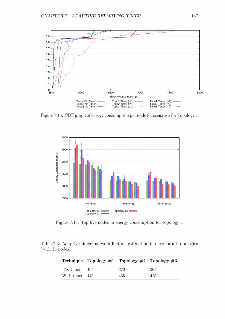
CHAPTER 7. ADAPTIVE REPORTING TIMER 147
0
0.1
0.2
0.3
0.4
0.5
0.6
0.7
0.8
0.9
1
5500 6000 6500 7000 7500 8000
Energy consumption (mJ)
Topo1-No TimerTopo2-No TimerTopo3-No Timer
Topo1-Timer (t=1)Topo2-Timer (t=1)Topo3-Timer (t=1)
Topo1-Timer (t=2)Topo2-Timer (t=2)Topo3-Timer (t=2)
Figure 7.15: CDF graph of energy consumption per node for scenarios for Topology 1
5500
6000
6500
7000
7500
8000
Ene
rgy
Con
sum
ptio
n (m
J)
Topology #1Topology #2
Topology #3
Timer (t=2)Timer (t=1)No Timer
Figure 7.16: Top five nodes in energy consumption for topology 1
Table 7.3: Adaptive timer: network lifetime estimation in days for all topologies(with 35 nodes)
Technique Topology #1 Topology #2 Topology #3
No timer 405 370 365With timer 445 435 425
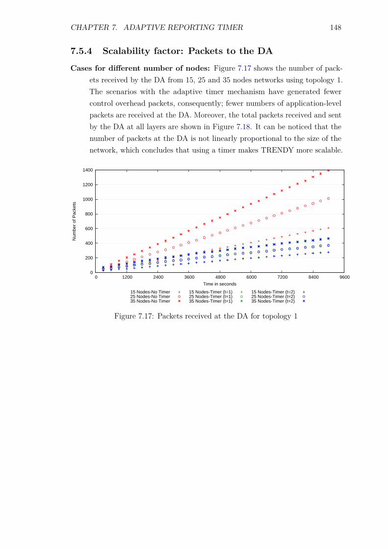
CHAPTER 7. ADAPTIVE REPORTING TIMER 148
7.5.4 Scalability factor: Packets to the DA
Cases for different number of nodes: Figure 7.17 shows the number of pack-ets received by the DA from 15, 25 and 35 nodes networks using topology 1.The scenarios with the adaptive timer mechanism have generated fewercontrol overhead packets, consequently; fewer numbers of application-levelpackets are received at the DA. Moreover, the total packets received and sentby the DA at all layers are shown in Figure 7.18. It can be noticed that thenumber of packets at the DA is not linearly proportional to the size of thenetwork, which concludes that using a timer makes TRENDY more scalable.
0
200
400
600
800
1000
1200
1400
0 1200 2400 3600 4800 6000 7200 8400 9600
Num
ber
of P
acke
ts
Time in seconds
15 Nodes-No Timer25 Nodes-No Timer35 Nodes-No Timer
15 Nodes-Timer (t=1)25 Nodes-Timer (t=1)35 Nodes-Timer (t=1)
15 Nodes-Timer (t=2)25 Nodes-Timer (t=2)35 Nodes-Timer (t=2)
Figure 7.17: Packets received at the DA for topology 1
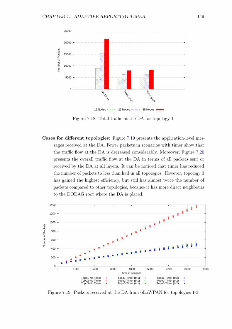
CHAPTER 7. ADAPTIVE REPORTING TIMER 149
0
5000
10000
15000
20000
25000
No Tim
er
Timer (t=1)
Timer (t=2)
Num
ber
of P
acke
ts
15 Nodes 25 Nodes 35 Nodes
Figure 7.18: Total traffic at the DA for topology 1
Cases for different topologies: Figure 7.19 presents the application-level mes-sages received at the DA. Fewer packets in scenarios with timer show thatthe traffic flow at the DA is decreased considerably. Moreover, Figure 7.20presents the overall traffic flow at the DA in terms of all packets sent orreceived by the DA at all layers. It can be noticed that timer has reducedthe number of packets to less than half in all topologies. However, topology 3has gained the highest efficiency, but still has almost twice the number ofpackets compared to other topologies, because it has more direct neighboursto the DODAG root where the DA is placed.
0
200
400
600
800
1000
1200
1400
0 1200 2400 3600 4800 6000 7200 8400 9600
Num
ber
of P
acke
ts
Time in seconds
Topo1-No TimerTopo2-No TimerTopo3-No Timer
Topo1-Timer (t=1)Topo2-Timer (t=1)Topo3-Timer (t=1)
Topo1-Timer (t=2)Topo2-Timer (t=2)Topo3-Timer (t=2)
Figure 7.19: Packets received at the DA from 6LoWPAN for topologies 1-3
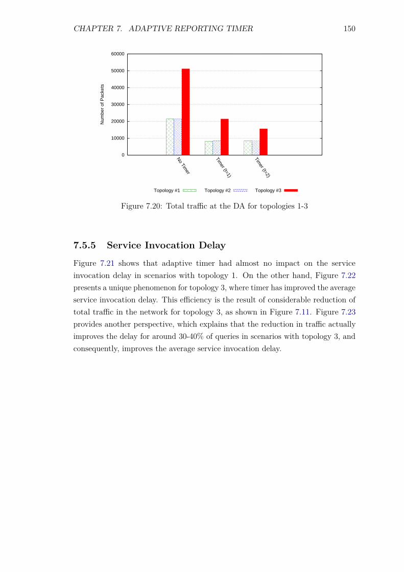
CHAPTER 7. ADAPTIVE REPORTING TIMER 150
0
10000
20000
30000
40000
50000
60000
No Tim
er
Timer (t=1)
Timer (t=2)
Num
ber
of P
acke
ts
Topology #1 Topology #2 Topology #3
Figure 7.20: Total traffic at the DA for topologies 1-3
7.5.5 Service Invocation Delay
Figure 7.21 shows that adaptive timer had almost no impact on the serviceinvocation delay in scenarios with topology 1. On the other hand, Figure 7.22presents a unique phenomenon for topology 3, where timer has improved the averageservice invocation delay. This efficiency is the result of considerable reduction oftotal traffic in the network for topology 3, as shown in Figure 7.11. Figure 7.23provides another perspective, which explains that the reduction in traffic actuallyimproves the delay for around 30-40% of queries in scenarios with topology 3, andconsequently, improves the average service invocation delay.
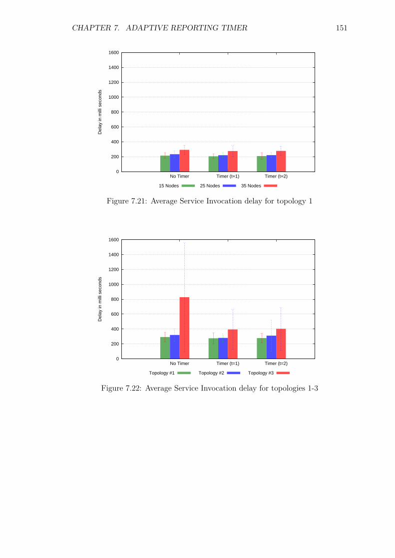
CHAPTER 7. ADAPTIVE REPORTING TIMER 151
0
200
400
600
800
1000
1200
1400
1600
No Timer Timer (t=1) Timer (t=2)
Del
ay in
mill
i sec
onds
15 Nodes 25 Nodes 35 Nodes
Figure 7.21: Average Service Invocation delay for topology 1
0
200
400
600
800
1000
1200
1400
1600
No Timer Timer (t=1) Timer (t=2)
Del
ay in
mill
i sec
onds
Topology #1 Topology #2 Topology #3
Figure 7.22: Average Service Invocation delay for topologies 1-3
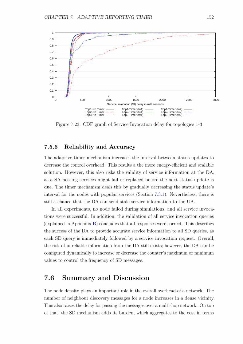
CHAPTER 7. ADAPTIVE REPORTING TIMER 152
0
0.1
0.2
0.3
0.4
0.5
0.6
0.7
0.8
0.9
1
0 500 1000 1500 2000 2500 3000
Service Invocation (SI) delay in milli seconds
Top1-No TimerTop2-No TimerTop3-No Timer
Top1-Timer (t=1)Top2-Timer (t=1)Top3-Timer (t=1)
Top1-Timer (t=2)Top2-Timer (t=2)Top3-Timer (t=2)
Figure 7.23: CDF graph of Service Invocation delay for topologies 1-3
7.5.6 Reliability and Accuracy
The adaptive timer mechanism increases the interval between status updates todecrease the control overhead. This results a the more energy-efficient and scalablesolution. However, this also risks the validity of service information at the DA,as a SA hosting services might fail or replaced before the next status update isdue. The timer mechanism deals this by gradually decreasing the status update’sinterval for the nodes with popular services (Section 7.3.1). Nevertheless, there isstill a chance that the DA can send stale service information to the UA.
In all experiments, no node failed during simulations, and all service invoca-tions were successful. In addition, the validation of all service invocation queries(explained in Appendix B) concludes that all responses were correct. This describesthe success of the DA to provide accurate service information to all SD queries, aseach SD query is immediately followed by a service invocation request. Overall,the risk of unreliable information from the DA still exists; however, the DA can beconfigured dynamically to increase or decrease the counter’s maximum or minimumvalues to control the frequency of SD messages.
7.6 Summary and Discussion
The node density plays an important role in the overall overhead of a network. Thenumber of neighbour discovery messages for a node increases in a dense vicinity.This also raises the delay for passing the messages over a multi-hop network. On topof that, the SD mechanism adds its burden, which aggregates to the cost in terms
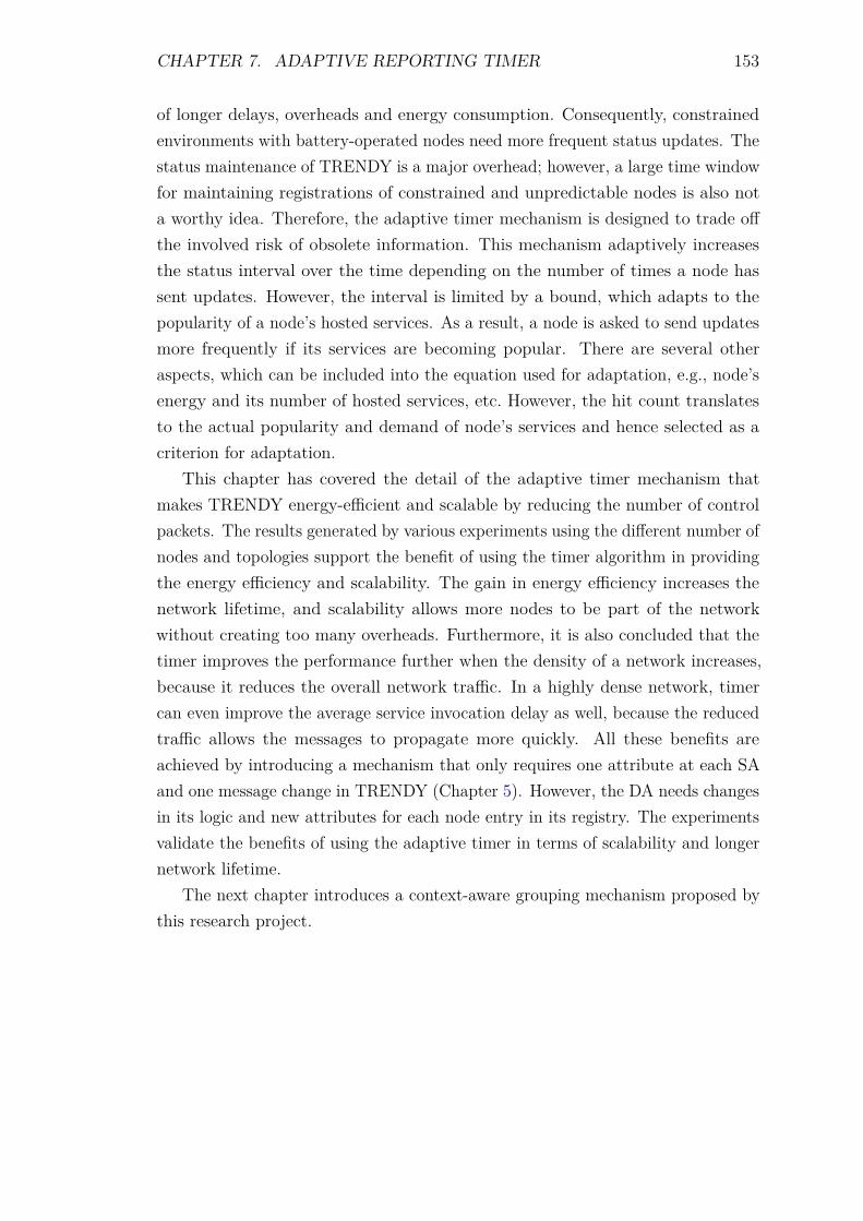
CHAPTER 7. ADAPTIVE REPORTING TIMER 153
of longer delays, overheads and energy consumption. Consequently, constrainedenvironments with battery-operated nodes need more frequent status updates. Thestatus maintenance of TRENDY is a major overhead; however, a large time windowfor maintaining registrations of constrained and unpredictable nodes is also nota worthy idea. Therefore, the adaptive timer mechanism is designed to trade offthe involved risk of obsolete information. This mechanism adaptively increasesthe status interval over the time depending on the number of times a node hassent updates. However, the interval is limited by a bound, which adapts to thepopularity of a node’s hosted services. As a result, a node is asked to send updatesmore frequently if its services are becoming popular. There are several otheraspects, which can be included into the equation used for adaptation, e.g., node’senergy and its number of hosted services, etc. However, the hit count translatesto the actual popularity and demand of node’s services and hence selected as acriterion for adaptation.
This chapter has covered the detail of the adaptive timer mechanism thatmakes TRENDY energy-efficient and scalable by reducing the number of controlpackets. The results generated by various experiments using the different number ofnodes and topologies support the benefit of using the timer algorithm in providingthe energy efficiency and scalability. The gain in energy efficiency increases thenetwork lifetime, and scalability allows more nodes to be part of the networkwithout creating too many overheads. Furthermore, it is also concluded that thetimer improves the performance further when the density of a network increases,because it reduces the overall network traffic. In a highly dense network, timercan even improve the average service invocation delay as well, because the reducedtraffic allows the messages to propagate more quickly. All these benefits areachieved by introducing a mechanism that only requires one attribute at each SAand one message change in TRENDY (Chapter 5). However, the DA needs changesin its logic and new attributes for each node entry in its registry. The experimentsvalidate the benefits of using the adaptive timer in terms of scalability and longernetwork lifetime.
The next chapter introduces a context-aware grouping mechanism proposed bythis research project.
Chapter 8
Context-aware Grouping
8.1 Introduction
The centralised architecture of the proposed solution (Chapter 5) requires theregistration and status maintenance updates to be received at the DA. However,this can lead to a single point of failure and also has a potential for bottleneckproblem for scalability. The problem is partially addressed by embedding theDA role in an edge router. This can tackle the single point of failure issue, asan edge router is a bridge between a 6LoWPAN and the Internet. Furthermore,adaptive timer (Chapter 7) decreases the control traffic, but the inherent problemof scalability with centralised architecture still exists as all control traffic flowstowards a single point. This chapter covers the detail of context-aware groupingtechnique, which solves the problem by localising the status maintenance task andprovides the basis to enable service composition paradigm.
8.2 Aims
Following are the aims of context-aware grouping:
1. Localise status maintenance: The main goal of the grouping scheme isto localise the traffic generated by status updates.
2. Efficient: It should not overwhelm the network by extra burden of groupingmessages, so grouping overhead should be minimum.
3. Resource awareness: The mechanism should not pose more requirementsto constrained devices. On the other hand, it should be able to intelligentlyuse the resources of highly capable devices.
4. Service Composition: It should address the demand of service compositionfor the IoT scenarios.
154
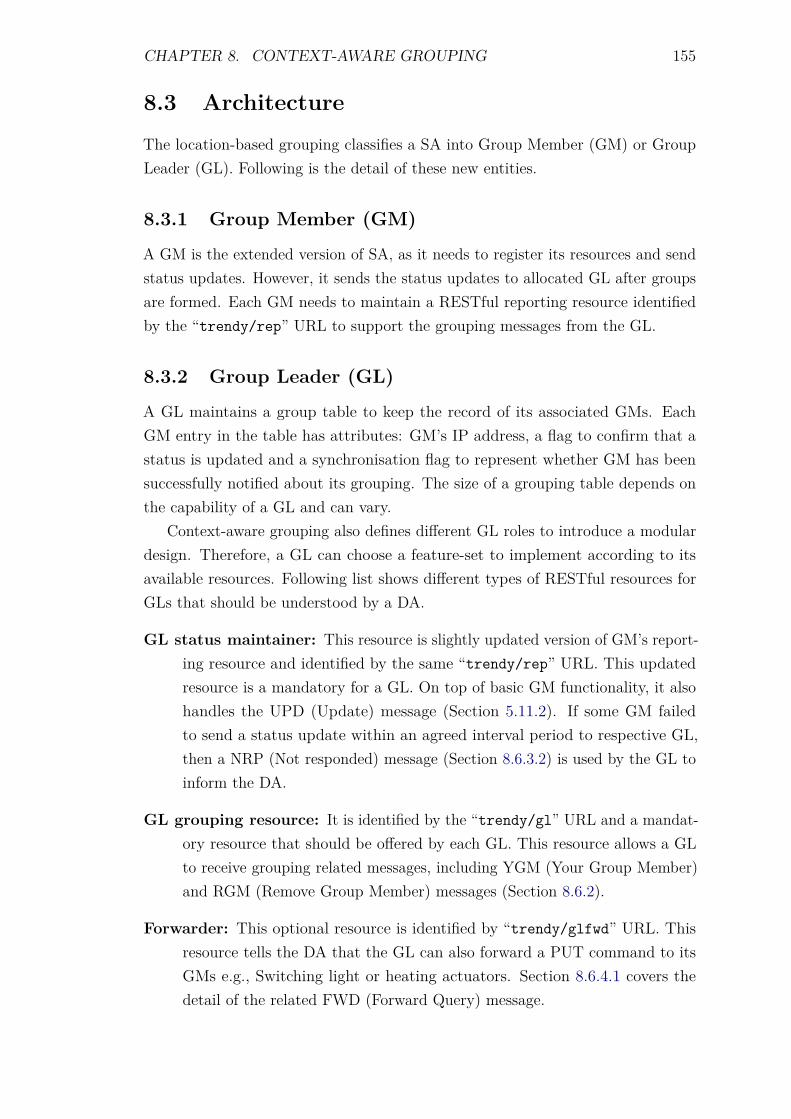
CHAPTER 8. CONTEXT-AWARE GROUPING 155
8.3 Architecture
The location-based grouping classifies a SA into Group Member (GM) or GroupLeader (GL). Following is the detail of these new entities.
8.3.1 Group Member (GM)
A GM is the extended version of SA, as it needs to register its resources and sendstatus updates. However, it sends the status updates to allocated GL after groupsare formed. Each GM needs to maintain a RESTful reporting resource identifiedby the “trendy/rep” URL to support the grouping messages from the GL.
8.3.2 Group Leader (GL)
A GL maintains a group table to keep the record of its associated GMs. EachGM entry in the table has attributes: GM’s IP address, a flag to confirm that astatus is updated and a synchronisation flag to represent whether GM has beensuccessfully notified about its grouping. The size of a grouping table depends onthe capability of a GL and can vary.
Context-aware grouping also defines different GL roles to introduce a modulardesign. Therefore, a GL can choose a feature-set to implement according to itsavailable resources. Following list shows different types of RESTful resources forGLs that should be understood by a DA.
GL status maintainer: This resource is slightly updated version of GM’s report-ing resource and identified by the same “trendy/rep” URL. This updatedresource is a mandatory for a GL. On top of basic GM functionality, it alsohandles the UPD (Update) message (Section 5.11.2). If some GM failedto send a status update within an agreed interval period to respective GL,then a NRP (Not responded) message (Section 8.6.3.2) is used by the GL toinform the DA.
GL grouping resource: It is identified by the “trendy/gl” URL and a mandat-ory resource that should be offered by each GL. This resource allows a GLto receive grouping related messages, including YGM (Your Group Member)and RGM (Remove Group Member) messages (Section 8.6.2).
Forwarder: This optional resource is identified by “trendy/glfwd” URL. Thisresource tells the DA that the GL can also forward a PUT command to itsGMs e.g., Switching light or heating actuators. Section 8.6.4.1 covers thedetail of the related FWD (Forward Query) message.
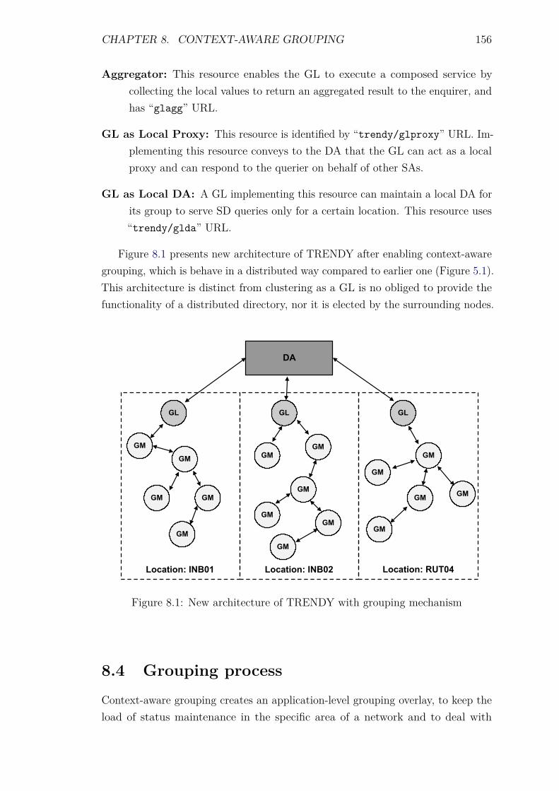
CHAPTER 8. CONTEXT-AWARE GROUPING 156
Aggregator: This resource enables the GL to execute a composed service bycollecting the local values to return an aggregated result to the enquirer, andhas “glagg” URL.
GL as Local Proxy: This resource is identified by “trendy/glproxy” URL. Im-plementing this resource conveys to the DA that the GL can act as a localproxy and can respond to the querier on behalf of other SAs.
GL as Local DA: A GL implementing this resource can maintain a local DA forits group to serve SD queries only for a certain location. This resource uses“trendy/glda” URL.
Figure 8.1 presents new architecture of TRENDY after enabling context-awaregrouping, which is behave in a distributed way compared to earlier one (Figure 5.1).This architecture is distinct from clustering as a GL is no obliged to provide thefunctionality of a distributed directory, nor it is elected by the surrounding nodes.
�� �� ��
��
��
��
��
�� ��
��
����
����
��
��
��
��
��
��
������� ���� ������� ���� ������� �����
Figure 8.1: New architecture of TRENDY with grouping mechanism
8.4 Grouping process
Context-aware grouping creates an application-level grouping overlay, to keep theload of status maintenance in the specific area of a network and to deal with
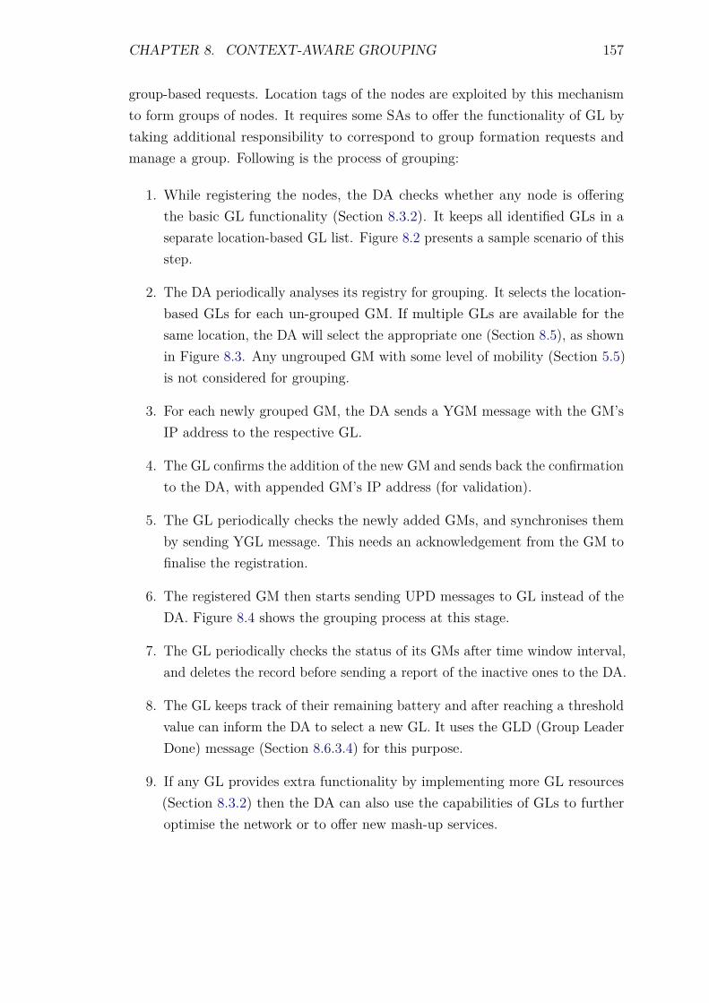
CHAPTER 8. CONTEXT-AWARE GROUPING 157
group-based requests. Location tags of the nodes are exploited by this mechanismto form groups of nodes. It requires some SAs to offer the functionality of GL bytaking additional responsibility to correspond to group formation requests andmanage a group. Following is the process of grouping:
1. While registering the nodes, the DA checks whether any node is offeringthe basic GL functionality (Section 8.3.2). It keeps all identified GLs in aseparate location-based GL list. Figure 8.2 presents a sample scenario of thisstep.
2. The DA periodically analyses its registry for grouping. It selects the location-based GLs for each un-grouped GM. If multiple GLs are available for thesame location, the DA will select the appropriate one (Section 8.5), as shownin Figure 8.3. Any ungrouped GM with some level of mobility (Section 5.5)is not considered for grouping.
3. For each newly grouped GM, the DA sends a YGM message with the GM’sIP address to the respective GL.
4. The GL confirms the addition of the new GM and sends back the confirmationto the DA, with appended GM’s IP address (for validation).
5. The GL periodically checks the newly added GMs, and synchronises themby sending YGL message. This needs an acknowledgement from the GM tofinalise the registration.
6. The registered GM then starts sending UPD messages to GL instead of theDA. Figure 8.4 shows the grouping process at this stage.
7. The GL periodically checks the status of its GMs after time window interval,and deletes the record before sending a report of the inactive ones to the DA.
8. The GL keeps track of their remaining battery and after reaching a thresholdvalue can inform the DA to select a new GL. It uses the GLD (Group LeaderDone) message (Section 8.6.3.4) for this purpose.
9. If any GL provides extra functionality by implementing more GL resources(Section 8.3.2) then the DA can also use the capabilities of GLs to furtheroptimise the network or to offer new mash-up services.
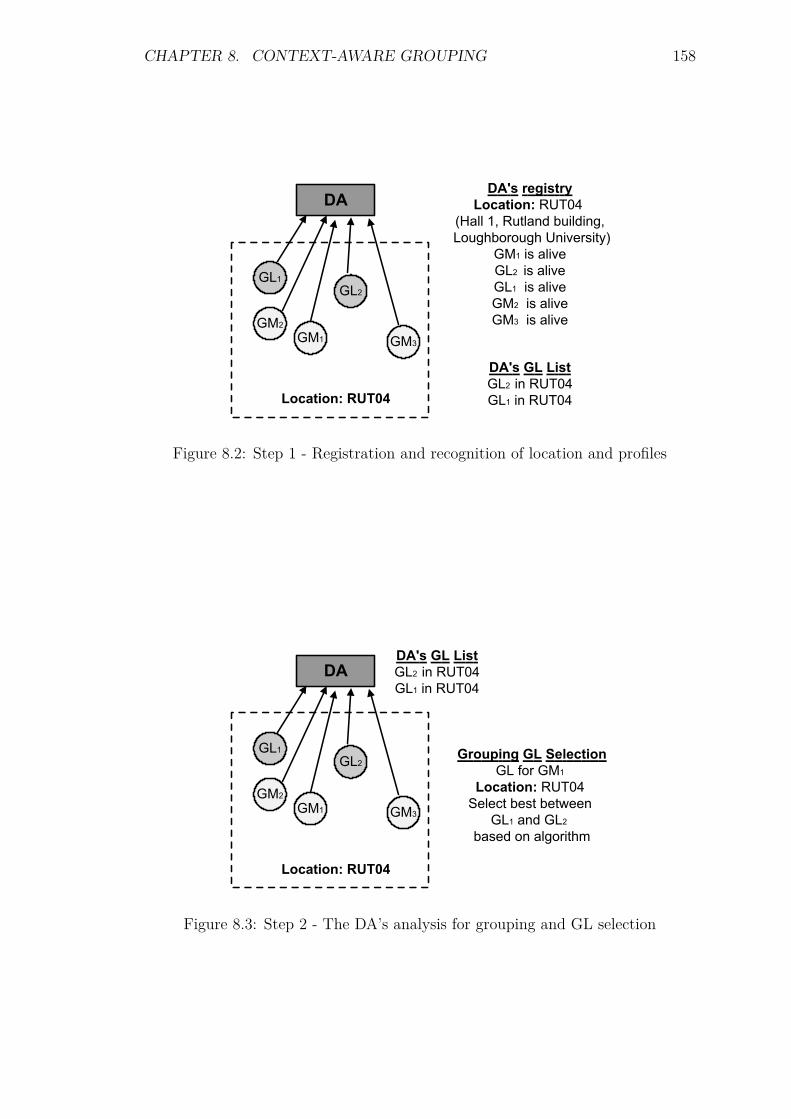
CHAPTER 8. CONTEXT-AWARE GROUPING 158
���
��
�������� �� ��
���
���
��� ���
���� �������������� ���
���� �� ������� ��������������������� ���������
��� �� �������� �� �������� �� �������� �� �������� �� �����
���� �� ������ �� ������ �� ���
Figure 8.2: Step 1 - Registration and recognition of location and profiles
���
��
�������� �� ��
���
���
��� ���
���� �� ������� � �� ���� � �� �
���� � �� ������� �� ��� ���
�������� �� ������� ���� ������
��� �� ���
����� � ���������
Figure 8.3: Step 2 - The DA’s analysis for grouping and GL selection
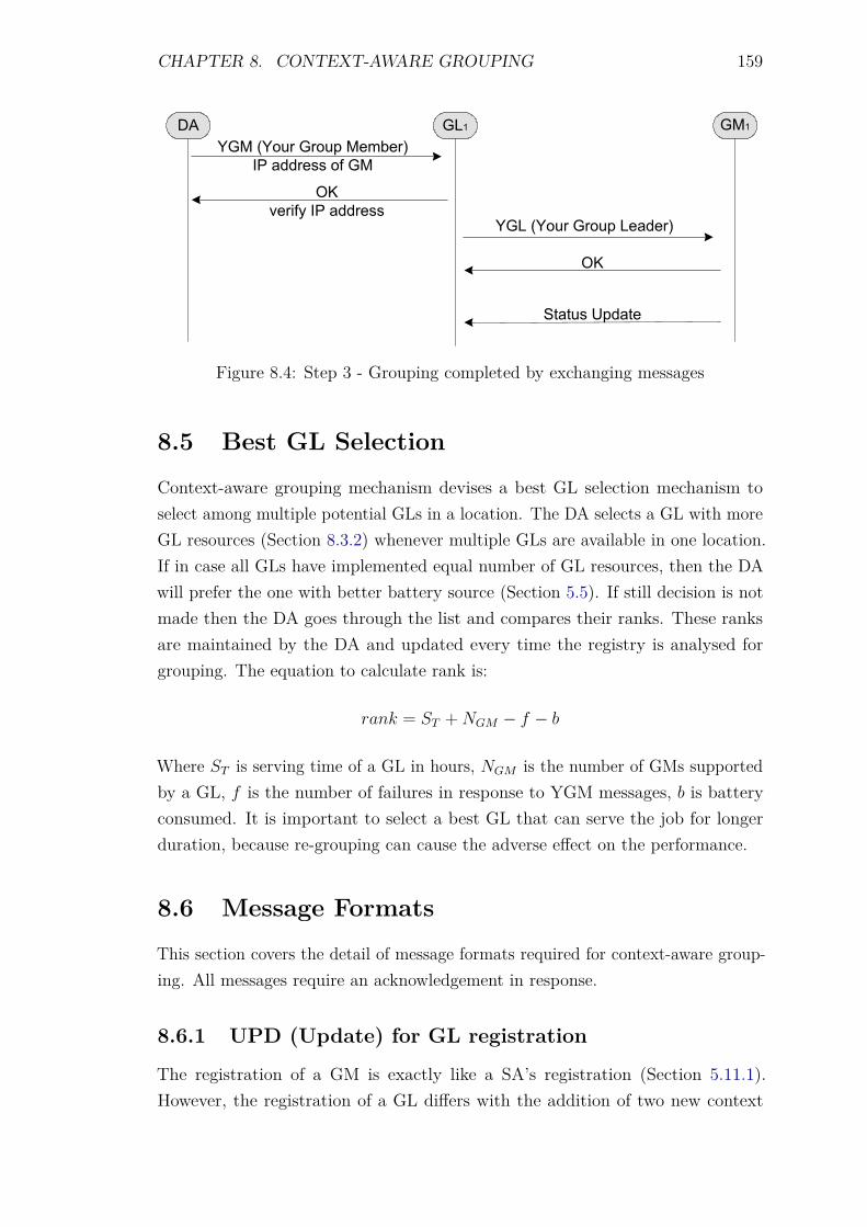
CHAPTER 8. CONTEXT-AWARE GROUPING 159
����� ���
��� ��� ��� � �� ���� ���� �� � ��
��� ���� �� ���� ��
��� ��� ��� � �� ��
��
����� �����
Figure 8.4: Step 3 - Grouping completed by exchanging messages
8.5 Best GL Selection
Context-aware grouping mechanism devises a best GL selection mechanism toselect among multiple potential GLs in a location. The DA selects a GL with moreGL resources (Section 8.3.2) whenever multiple GLs are available in one location.If in case all GLs have implemented equal number of GL resources, then the DAwill prefer the one with better battery source (Section 5.5). If still decision is notmade then the DA goes through the list and compares their ranks. These ranksare maintained by the DA and updated every time the registry is analysed forgrouping. The equation to calculate rank is:
rank = ST + NGM − f − b
Where ST is serving time of a GL in hours, NGM is the number of GMs supportedby a GL, f is the number of failures in response to YGM messages, b is batteryconsumed. It is important to select a best GL that can serve the job for longerduration, because re-grouping can cause the adverse effect on the performance.
8.6 Message Formats
This section covers the detail of message formats required for context-aware group-ing. All messages require an acknowledgement in response.
8.6.1 UPD (Update) for GL registration
The registration of a GM is exactly like a SA’s registration (Section 5.11.1).However, the registration of a GL differs with the addition of two new context
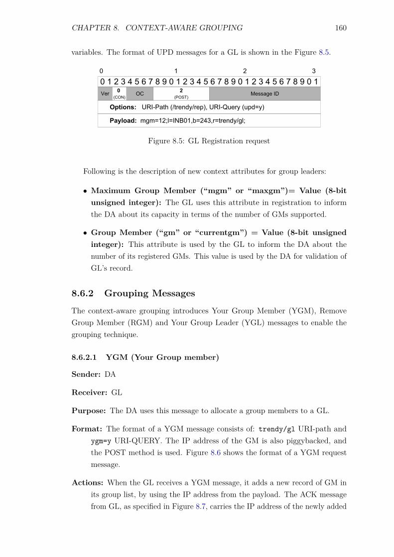
CHAPTER 8. CONTEXT-AWARE GROUPING 160
variables. The format of UPD messages for a GL is shown in the Figure 8.5.
� � � � � � � � � � � � � � � � � � � � � � � � � ��� ��
�������� �������� ��� ����� ���� ���� !� � �!��"��
����� #$#"��%&"�'(���)"���� "� �����$&%
� � � �
���'�
����,-�
.�//�$� �0
Figure 8.5: GL Registration request
Following is the description of new context attributes for group leaders:
• Maximum Group Member (“mgm” or “maxgm”)= Value (8-bitunsigned integer): The GL uses this attribute in registration to informthe DA about its capacity in terms of the number of GMs supported.
• Group Member (“gm” or “currentgm”) = Value (8-bit unsignedinteger): This attribute is used by the GL to inform the DA about thenumber of its registered GMs. This value is used by the DA for validation ofGL’s record.
8.6.2 Grouping Messages
The context-aware grouping introduces Your Group Member (YGM), RemoveGroup Member (RGM) and Your Group Leader (YGL) messages to enable thegrouping technique.
8.6.2.1 YGM (Your Group member)
Sender: DA
Receiver: GL
Purpose: The DA uses this message to allocate a group members to a GL.
Format: The format of a YGM message consists of: trendy/gl URI-path andygm=y URI-QUERY. The IP address of the GM is also piggybacked, andthe POST method is used. Figure 8.6 shows the format of a YGM requestmessage.
Actions: When the GL receives a YGM message, it adds a new record of GM inits group list, by using the IP address from the payload. The ACK messagefrom GL, as specified in Figure 8.7, carries the IP address of the newly added
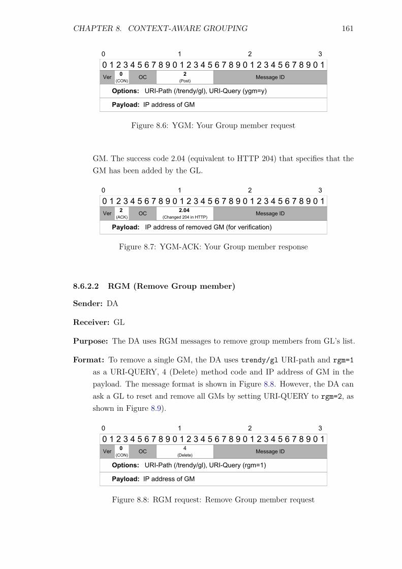
CHAPTER 8. CONTEXT-AWARE GROUPING 161
� � � � � � � � � � � � � � � � � � � � � � � � � ��� ��
�������� �������� ��� �������� ����!"� � ���#$��
����� �� ��� �%% &' ()
� � � �
���+�
���&%��
)�%%��� �-
Figure 8.6: YGM: Your Group member request
GM. The success code 2.04 (equivalent to HTTP 204) that specifies that theGM has been added by the GL.
� � � � � � � � � � � � � � � � � � � � � � � � � ��� ��
�������� �� ��� ��� �� ������ �� ��� �� ���������
� � � �
��"�#
����%��&�� ��� �� '((�
�����&� �)
Figure 8.7: YGM-ACK: Your Group member response
8.6.2.2 RGM (Remove Group member)
Sender: DA
Receiver: GL
Purpose: The DA uses RGM messages to remove group members from GL’s list.
Format: To remove a single GM, the DA uses trendy/gl URI-path and rgm=1as a URI-QUERY, 4 (Delete) method code and IP address of GM in thepayload. The message format is shown in Figure 8.8. However, the DA canask a GL to reset and remove all GMs by setting URI-QUERY to rgm=2, asshown in Figure 8.9).
� � � � � � � � � � � � � � � � � � � � � � � � � ��� ��
�������� �������� ��� �������� ����!"� � � �#$��
����� �� ��� �%% &' ()
� � � �
���+�
��-������
)�%%��� �-
Figure 8.8: RGM request: Remove Group member request
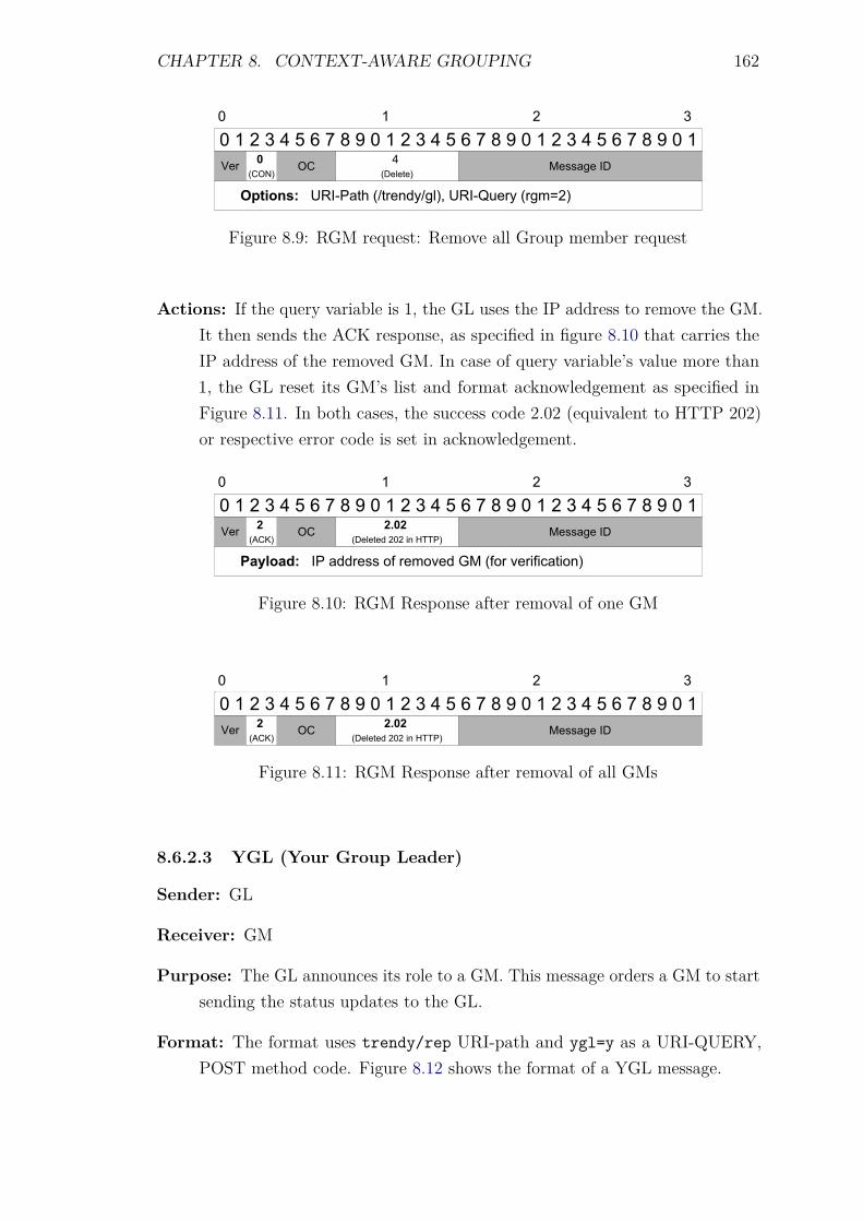
CHAPTER 8. CONTEXT-AWARE GROUPING 162
� � � � � � � � � � � � � � � � � � � � � � � � � ��� ��
�������� �������� ��� �������� ����!"� � � �#$��
� � � �
����&�
��(������
)�**��� �(
Figure 8.9: RGM request: Remove all Group member request
Actions: If the query variable is 1, the GL uses the IP address to remove the GM.It then sends the ACK response, as specified in figure 8.10 that carries theIP address of the removed GM. In case of query variable’s value more than1, the GL reset its GM’s list and format acknowledgement as specified inFigure 8.11. In both cases, the success code 2.02 (equivalent to HTTP 202)or respective error code is set in acknowledgement.
� � � � � � � � � � � � � � � � � � � � � � � � � ��� ��
�������� �� ��� ��� �� ������ �� ��� �� ���������
� � � �
��"�#
����%�&���� ��� �� '((�
�����)� �%
Figure 8.10: RGM Response after removal of one GM
� � � � � � � � � � � � � � � � � � � � � � � � � ��� ��
� � � �
������
������������ ��� �� �����
�� !"� #�
Figure 8.11: RGM Response after removal of all GMs
8.6.2.3 YGL (Your Group Leader)
Sender: GL
Receiver: GM
Purpose: The GL announces its role to a GM. This message orders a GM to startsending the status updates to the GL.
Format: The format uses trendy/rep URI-path and ygl=y as a URI-QUERY,POST method code. Figure 8.12 shows the format of a YGL message.
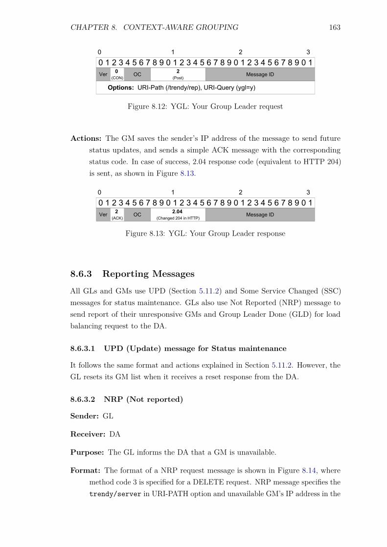
CHAPTER 8. CONTEXT-AWARE GROUPING 163
� � � � � � � � � � � � � � � � � � � � � � � � � ��� ��
�������� �������� ��� ����� ���� ���� !� � ��"#$��
� � � �
����&�
��()��
*�))�"� �+
Figure 8.12: YGL: Your Group Leader request
Actions: The GM saves the sender’s IP address of the message to send futurestatus updates, and sends a simple ACK message with the correspondingstatus code. In case of success, 2.04 response code (equivalent to HTTP 204)is sent, as shown in Figure 8.13.
� � � � � � � � � � � � � � � � � � � � � � � � � ��� ��
� � � �
������
������������ ��� �� �����
�� ��� !"
Figure 8.13: YGL: Your Group Leader response
8.6.3 Reporting Messages
All GLs and GMs use UPD (Section 5.11.2) and Some Service Changed (SSC)messages for status maintenance. GLs also use Not Reported (NRP) message tosend report of their unresponsive GMs and Group Leader Done (GLD) for loadbalancing request to the DA.
8.6.3.1 UPD (Update) message for Status maintenance
It follows the same format and actions explained in Section 5.11.2. However, theGL resets its GM list when it receives a reset response from the DA.
8.6.3.2 NRP (Not reported)
Sender: GL
Receiver: DA
Purpose: The GL informs the DA that a GM is unavailable.
Format: The format of a NRP request message is shown in Figure 8.14, wheremethod code 3 is specified for a DELETE request. NRP message specifies thetrendy/server in URI-PATH option and unavailable GM’s IP address in the
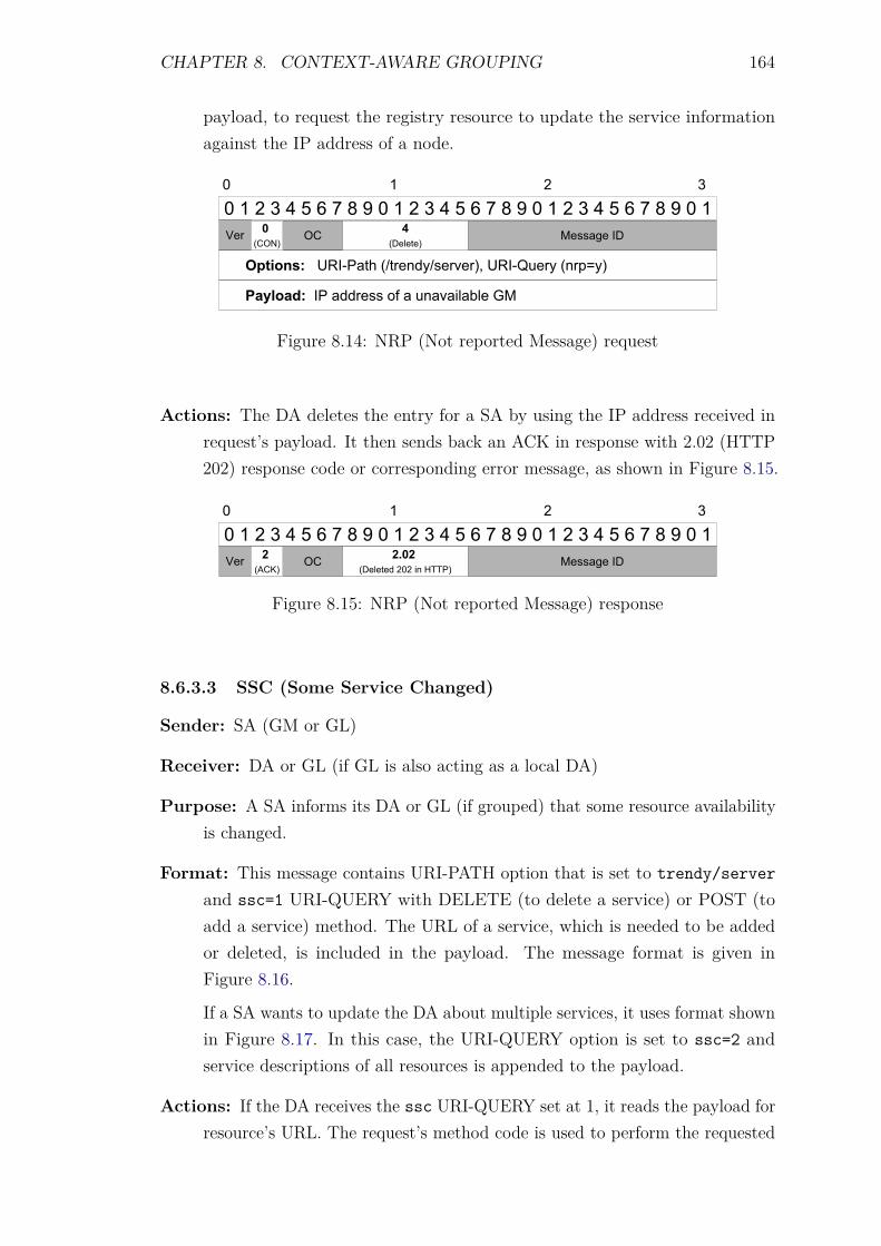
CHAPTER 8. CONTEXT-AWARE GROUPING 164
payload, to request the registry resource to update the service informationagainst the IP address of a node.
� � � � � � � � � � � � � � � � � � � � � � � � � ��� ��
�������� �������� ��� ������� �� � ����!"� � �� #$��
����� �� ��� ��� %& � "����'(�)(� *+
� � � �
���-�
��/�(����
+����0� �/
Figure 8.14: NRP (Not reported Message) request
Actions: The DA deletes the entry for a SA by using the IP address received inrequest’s payload. It then sends back an ACK in response with 2.02 (HTTP202) response code or corresponding error message, as shown in Figure 8.15.
� � � � � � � � � � � � � � � � � � � � � � � � � ��� ��
� � � �
������
������������ ��� �� �����
�� !"� #�
Figure 8.15: NRP (Not reported Message) response
8.6.3.3 SSC (Some Service Changed)
Sender: SA (GM or GL)
Receiver: DA or GL (if GL is also acting as a local DA)
Purpose: A SA informs its DA or GL (if grouped) that some resource availabilityis changed.
Format: This message contains URI-PATH option that is set to trendy/serverand ssc=1 URI-QUERY with DELETE (to delete a service) or POST (toadd a service) method. The URL of a service, which is needed to be addedor deleted, is included in the payload. The message format is given inFigure 8.16.
If a SA wants to update the DA about multiple services, it uses format shownin Figure 8.17. In this case, the URI-QUERY option is set to ssc=2 andservice descriptions of all resources is appended to the payload.
Actions: If the DA receives the ssc URI-QUERY set at 1, it reads the payload forresource’s URL. The request’s method code is used to perform the requested
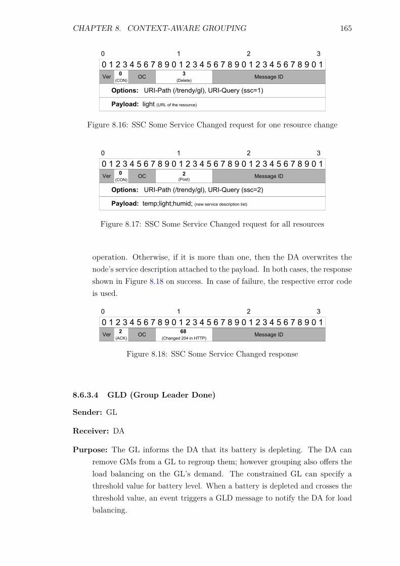
CHAPTER 8. CONTEXT-AWARE GROUPING 165
� � � � � � � � � � � � � � � � � � � � � � � � � ��� ��
�������� �������� ��� �������� ����!"� � �##$%��
����� �&��� ���' () ��� �#(" $��
� � � �
���+�
��-������
.�##��� �-
Figure 8.16: SSC Some Service Changed request for one resource change
� � � � � � � � � � � � � � � � � � � � � � � � � ��� ��
�������� �������� ��� �������� ����!"� � �##$%��
����� ��&'(�)���(�"&)�( ���* #� +)$� ��#$ )'�),� �)#��
� � � �
���.�
���,#�� 0�##��� �1
Figure 8.17: SSC Some Service Changed request for all resources
operation. Otherwise, if it is more than one, then the DA overwrites thenode’s service description attached to the payload. In both cases, the responseshown in Figure 8.18 on success. In case of failure, the respective error codeis used.
� � � � � � � � � � � � � � � � � � � � � � � � � ��� ��
� � � �
������
���������� ��� �� �����
�� ��� !"
Figure 8.18: SSC Some Service Changed response
8.6.3.4 GLD (Group Leader Done)
Sender: GL
Receiver: DA
Purpose: The GL informs the DA that its battery is depleting. The DA canremove GMs from a GL to regroup them; however grouping also offers theload balancing on the GL’s demand. The constrained GL can specify athreshold value for battery level. When a battery is depleted and crosses thethreshold value, an event triggers a GLD message to notify the DA for loadbalancing.
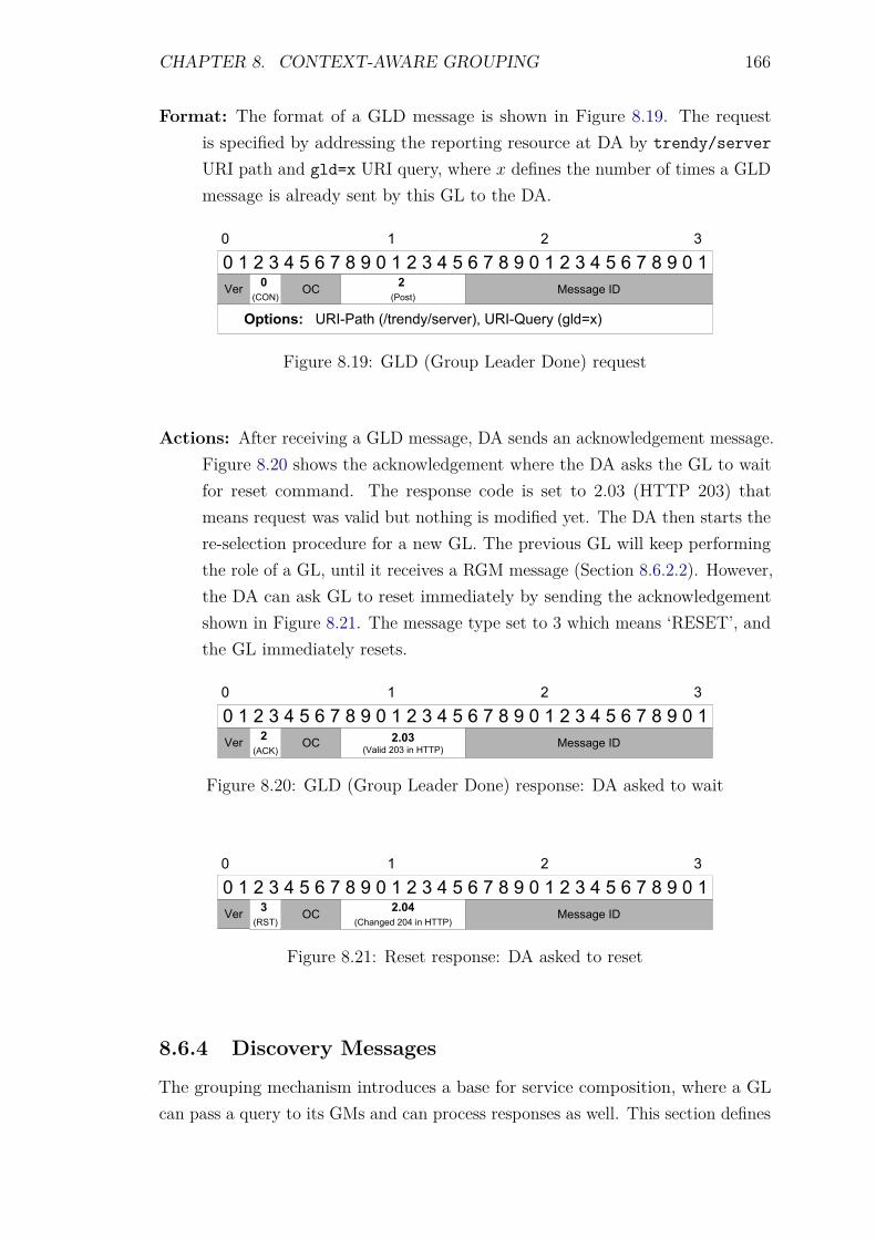
CHAPTER 8. CONTEXT-AWARE GROUPING 166
Format: The format of a GLD message is shown in Figure 8.19. The requestis specified by addressing the reporting resource at DA by trendy/serverURI path and gld=x URI query, where x defines the number of times a GLDmessage is already sent by this GL to the DA.
� � � � � � � � � � � � � � � � � � � � � � � � � ��� ��
�������� �������� ��� ������� �� � ����!"� � �#$�%&�
� � � �
����(�
��*���
+����#� �,
Figure 8.19: GLD (Group Leader Done) request
Actions: After receiving a GLD message, DA sends an acknowledgement message.Figure 8.20 shows the acknowledgement where the DA asks the GL to waitfor reset command. The response code is set to 2.03 (HTTP 203) thatmeans request was valid but nothing is modified yet. The DA then starts there-selection procedure for a new GL. The previous GL will keep performingthe role of a GL, until it receives a RGM message (Section 8.6.2.2). However,the DA can ask GL to reset immediately by sending the acknowledgementshown in Figure 8.21. The message type set to 3 which means ‘RESET’, andthe GL immediately resets.
� � � � � � � � � � � � � � � � � � � � � � � � � ��� ��
� � � �
������
���������� ��� �� ����� ����� � !"
Figure 8.20: GLD (Group Leader Done) response: DA asked to wait
� � � � � � � � � � � � � � � � � � � � � � � � � ��� ��
� � � �
������
������������ ��� �� �����
�� ��� !"
Figure 8.21: Reset response: DA asked to reset
8.6.4 Discovery Messages
The grouping mechanism introduces a base for service composition, where a GLcan pass a query to its GMs and can process responses as well. This section defines
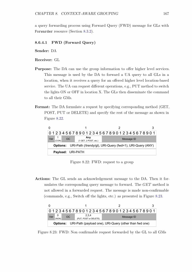
CHAPTER 8. CONTEXT-AWARE GROUPING 167
a query forwarding process using Forward Query (FWD) message for GLs withForwarder resource (Section 8.3.2).
8.6.4.1 FWD (Forward Query)
Sender: DA
Receiver: GL
Purpose: The DA can use the group information to offer higher level services.This message is used by the DA to forward a UA query to all GLs in alocation, when it receives a query for an offered higher level location-basedservice. The UA can request different operations, e.g., PUT method to switchthe lights ON or OFF in location X. The GLs then disseminate the commandto all their GMs.
Format: The DA formulate a request by specifying corresponding method (GET,POST, PUT or DELETE) and specify the rest of the message as shown inFigure 8.22.
� � � � � � � � � � � � � � � � � � � � � � � � � ��� ��
�������� �������� ��� �������� ����!"� � �#$�%�� ����!"� � �&'(�
����� �����&)*
� � � �
����'�
��� -.) � ��/) ��01�
2�33��� �4
Figure 8.22: FWD: request to a group
Actions: The GL sends an acknowledgement message to the DA. Then it for-mulates the corresponding query message to forward. The GET method isnot allowed in a forwarded request. The message is made non-confirmable(commands, e.g., Switch off the lights, etc.) as presented in Figure 8.23.
� � � � � � � � � � � � � � � � � � � � � � � � � ��� ��
�������� �������� �������� ���� ����!"� � ����� ���� #$� ����
� � � �
��&�&�
� � ����( ��)( � *+,+(+�
-�..�/� �*
Figure 8.23: FWD: Non confirmable request forwarded by the GL to all GMs
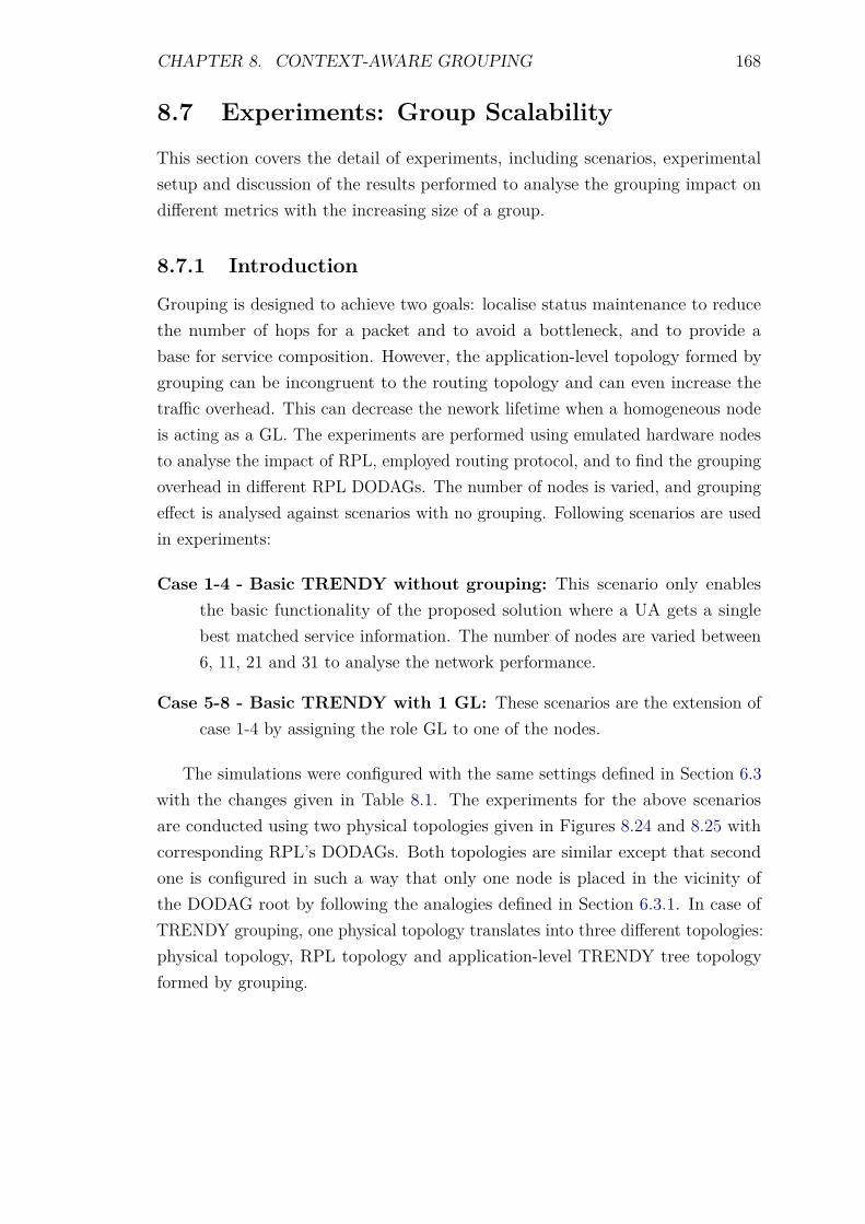
CHAPTER 8. CONTEXT-AWARE GROUPING 168
8.7 Experiments: Group Scalability
This section covers the detail of experiments, including scenarios, experimentalsetup and discussion of the results performed to analyse the grouping impact ondifferent metrics with the increasing size of a group.
8.7.1 Introduction
Grouping is designed to achieve two goals: localise status maintenance to reducethe number of hops for a packet and to avoid a bottleneck, and to provide abase for service composition. However, the application-level topology formed bygrouping can be incongruent to the routing topology and can even increase thetraffic overhead. This can decrease the nework lifetime when a homogeneous nodeis acting as a GL. The experiments are performed using emulated hardware nodesto analyse the impact of RPL, employed routing protocol, and to find the groupingoverhead in different RPL DODAGs. The number of nodes is varied, and groupingeffect is analysed against scenarios with no grouping. Following scenarios are usedin experiments:
Case 1-4 - Basic TRENDY without grouping: This scenario only enablesthe basic functionality of the proposed solution where a UA gets a singlebest matched service information. The number of nodes are varied between6, 11, 21 and 31 to analyse the network performance.
Case 5-8 - Basic TRENDY with 1 GL: These scenarios are the extension ofcase 1-4 by assigning the role GL to one of the nodes.
The simulations were configured with the same settings defined in Section 6.3with the changes given in Table 8.1. The experiments for the above scenariosare conducted using two physical topologies given in Figures 8.24 and 8.25 withcorresponding RPL’s DODAGs. Both topologies are similar except that secondone is configured in such a way that only one node is placed in the vicinity ofthe DODAG root by following the analogies defined in Section 6.3.1. In case ofTRENDY grouping, one physical topology translates into three different topologies:physical topology, RPL topology and application-level TRENDY tree topologyformed by grouping.
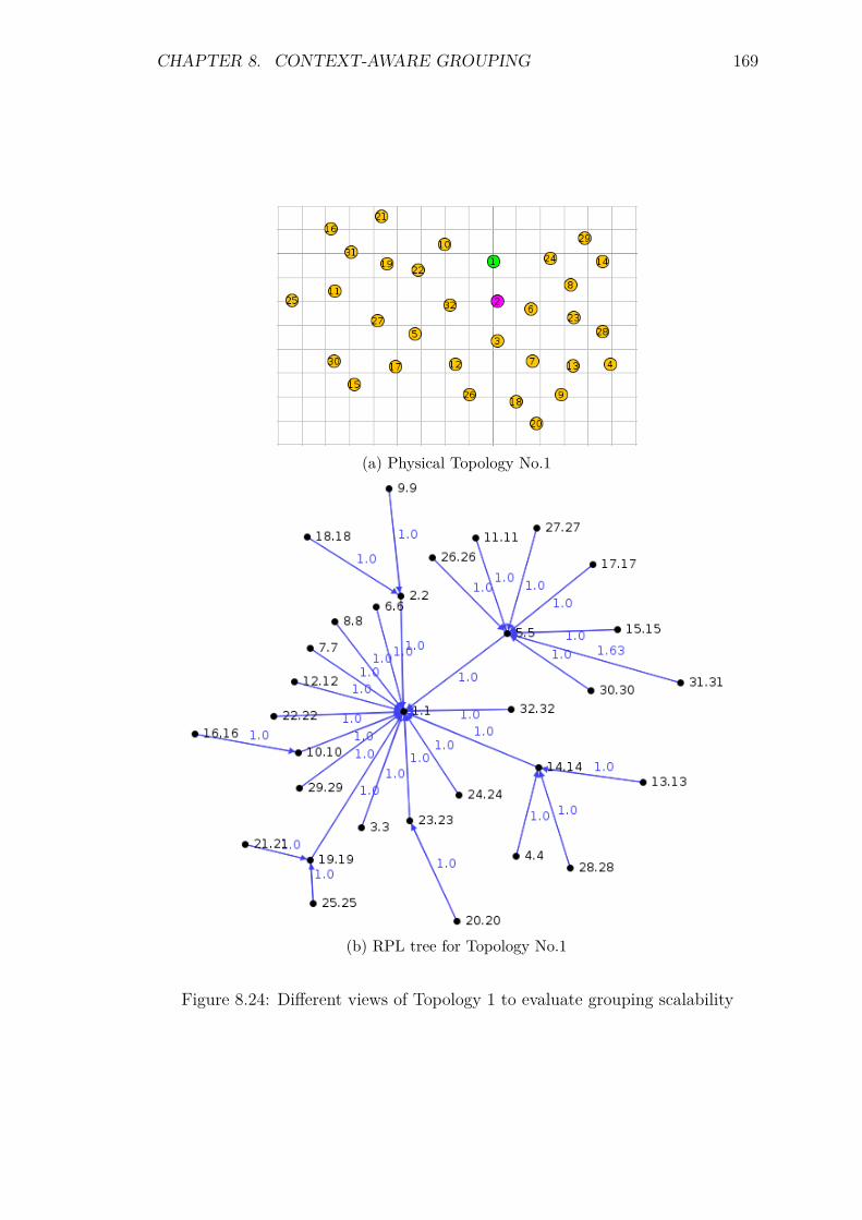
CHAPTER 8. CONTEXT-AWARE GROUPING 169
(a) Physical Topology No.1
(b) RPL tree for Topology No.1
Figure 8.24: Different views of Topology 1 to evaluate grouping scalability

CHAPTER 8. CONTEXT-AWARE GROUPING 170
(a) Physical Topology No.2
(b) RPL tree for Topology No.2
Figure 8.25: Different views of Topology 2 to evaluate grouping scalability
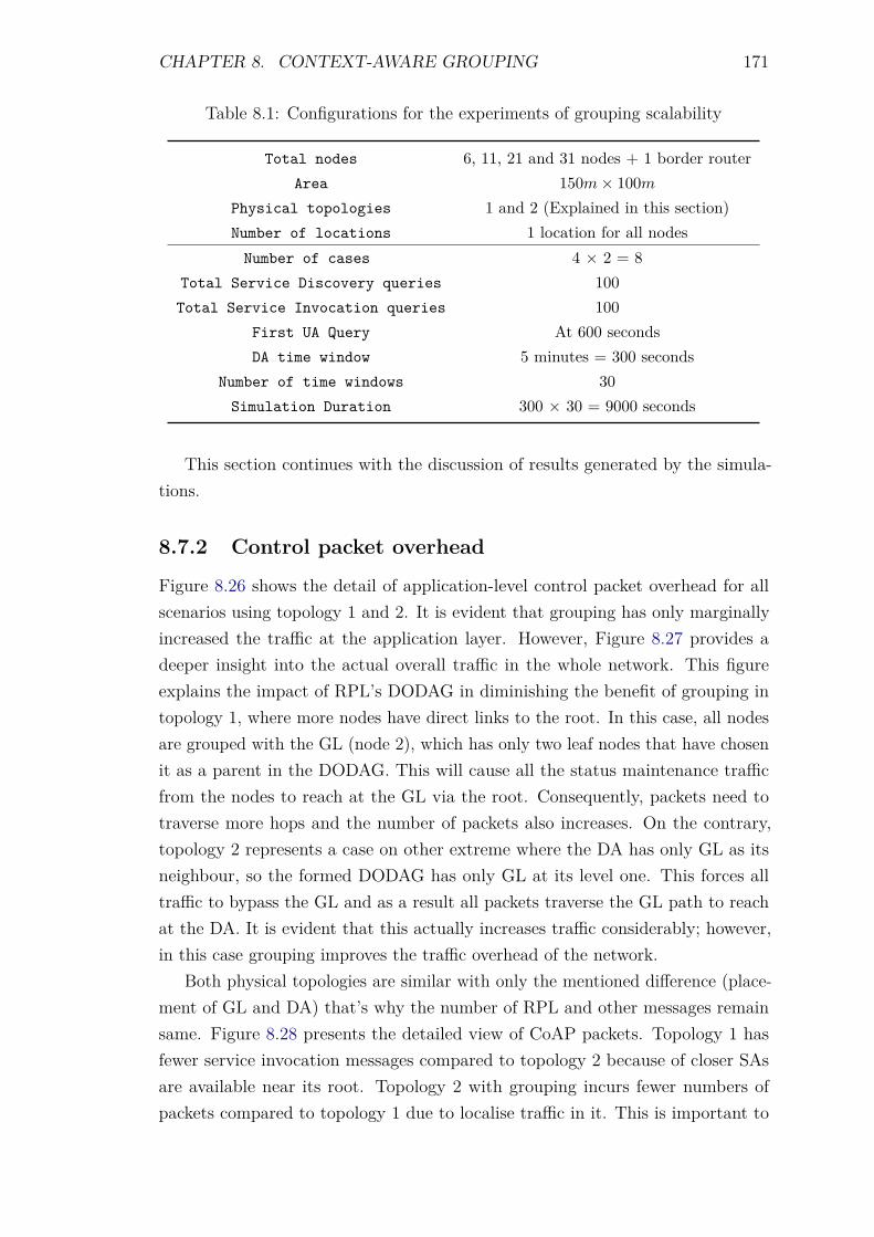
CHAPTER 8. CONTEXT-AWARE GROUPING 171
Table 8.1: Configurations for the experiments of grouping scalability
Total nodes 6, 11, 21 and 31 nodes + 1 border routerArea 150m× 100m
Physical topologies 1 and 2 (Explained in this section)Number of locations 1 location for all nodes
Number of cases 4 × 2 = 8Total Service Discovery queries 100Total Service Invocation queries 100
First UA Query At 600 secondsDA time window 5 minutes = 300 seconds
Number of time windows 30Simulation Duration 300 × 30 = 9000 seconds
This section continues with the discussion of results generated by the simula-tions.
8.7.2 Control packet overhead
Figure 8.26 shows the detail of application-level control packet overhead for allscenarios using topology 1 and 2. It is evident that grouping has only marginallyincreased the traffic at the application layer. However, Figure 8.27 provides adeeper insight into the actual overall traffic in the whole network. This figureexplains the impact of RPL’s DODAG in diminishing the benefit of grouping intopology 1, where more nodes have direct links to the root. In this case, all nodesare grouped with the GL (node 2), which has only two leaf nodes that have chosenit as a parent in the DODAG. This will cause all the status maintenance trafficfrom the nodes to reach at the GL via the root. Consequently, packets need totraverse more hops and the number of packets also increases. On the contrary,topology 2 represents a case on other extreme where the DA has only GL as itsneighbour, so the formed DODAG has only GL at its level one. This forces alltraffic to bypass the GL and as a result all packets traverse the GL path to reachat the DA. It is evident that this actually increases traffic considerably; however,in this case grouping improves the traffic overhead of the network.
Both physical topologies are similar with only the mentioned difference (place-ment of GL and DA) that’s why the number of RPL and other messages remainsame. Figure 8.28 presents the detailed view of CoAP packets. Topology 1 hasfewer service invocation messages compared to topology 2 because of closer SAsare available near its root. Topology 2 with grouping incurs fewer numbers ofpackets compared to topology 1 due to localise traffic in it. This is important to
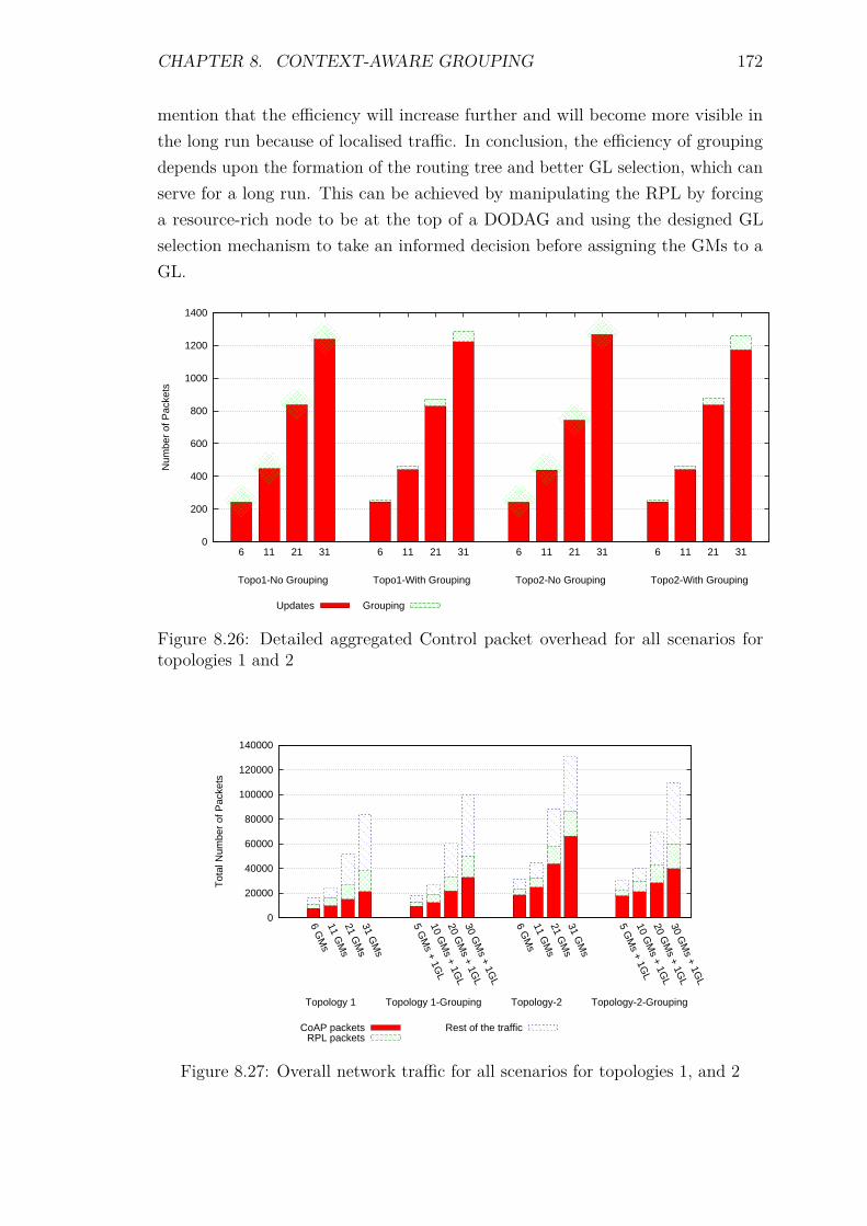
CHAPTER 8. CONTEXT-AWARE GROUPING 172
mention that the efficiency will increase further and will become more visible inthe long run because of localised traffic. In conclusion, the efficiency of groupingdepends upon the formation of the routing tree and better GL selection, which canserve for a long run. This can be achieved by manipulating the RPL by forcinga resource-rich node to be at the top of a DODAG and using the designed GLselection mechanism to take an informed decision before assigning the GMs to aGL.
0
200
400
600
800
1000
1200
1400
6 11 21 31 6 11 21 31 6 11 21 31 6 11 21 31
Num
ber
of P
acke
ts
Updates Grouping
Topo2-With GroupingTopo2-No GroupingTopo1-With GroupingTopo1-No Grouping
Figure 8.26: Detailed aggregated Control packet overhead for all scenarios fortopologies 1 and 2
0
20000
40000
60000
80000
100000
120000
140000
6 GM
s11 G
Ms
21 GM
s31 G
Ms
5 GM
s + 1GL
10 GM
s + 1GL
20 GM
s + 1GL
30 GM
s + 1GL
6 GM
s11 G
Ms
21 GM
s31 G
Ms
5 GM
s + 1GL
10 GM
s + 1GL
20 GM
s + 1GL
30 GM
s + 1GL
Tot
al N
umbe
r of
Pac
kets
CoAP packetsRPL packets
Rest of the traffic
Topology-2-GroupingTopology-2Topology 1-GroupingTopology 1
Figure 8.27: Overall network traffic for all scenarios for topologies 1, and 2
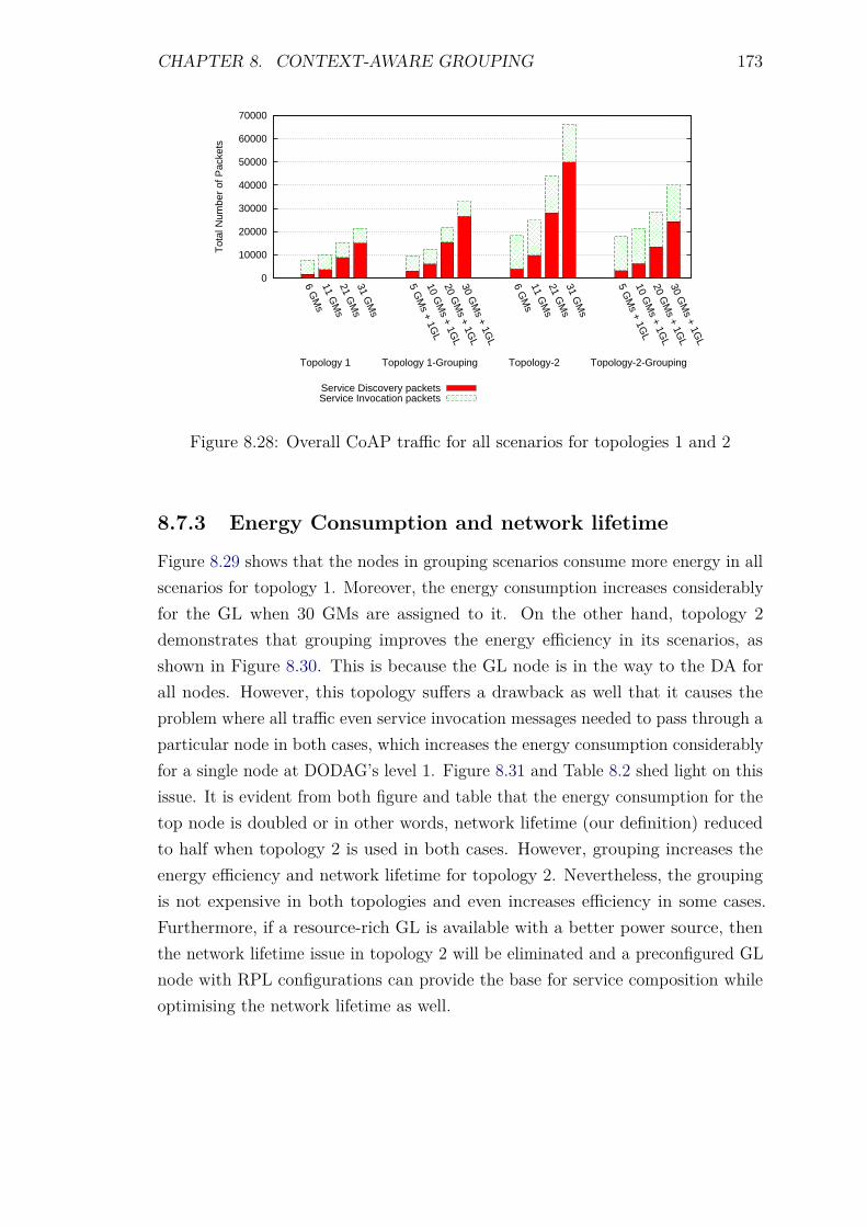
CHAPTER 8. CONTEXT-AWARE GROUPING 173
0
10000
20000
30000
40000
50000
60000
70000
6 GM
s11 G
Ms
21 GM
s31 G
Ms
5 GM
s + 1GL
10 GM
s + 1GL
20 GM
s + 1GL
30 GM
s + 1GL
6 GM
s11 G
Ms
21 GM
s31 G
Ms
5 GM
s + 1GL
10 GM
s + 1GL
20 GM
s + 1GL
30 GM
s + 1GL
Tot
al N
umbe
r of
Pac
kets
Service Discovery packetsService Invocation packets
Topology-2-GroupingTopology-2Topology 1-GroupingTopology 1
Figure 8.28: Overall CoAP traffic for all scenarios for topologies 1 and 2
8.7.3 Energy Consumption and network lifetime
Figure 8.29 shows that the nodes in grouping scenarios consume more energy in allscenarios for topology 1. Moreover, the energy consumption increases considerablyfor the GL when 30 GMs are assigned to it. On the other hand, topology 2demonstrates that grouping improves the energy efficiency in its scenarios, asshown in Figure 8.30. This is because the GL node is in the way to the DA forall nodes. However, this topology suffers a drawback as well that it causes theproblem where all traffic even service invocation messages needed to pass through aparticular node in both cases, which increases the energy consumption considerablyfor a single node at DODAG’s level 1. Figure 8.31 and Table 8.2 shed light on thisissue. It is evident from both figure and table that the energy consumption for thetop node is doubled or in other words, network lifetime (our definition) reducedto half when topology 2 is used in both cases. However, grouping increases theenergy efficiency and network lifetime for topology 2. Nevertheless, the groupingis not expensive in both topologies and even increases efficiency in some cases.Furthermore, if a resource-rich GL is available with a better power source, thenthe network lifetime issue in topology 2 will be eliminated and a preconfigured GLnode with RPL configurations can provide the base for service composition whileoptimising the network lifetime as well.
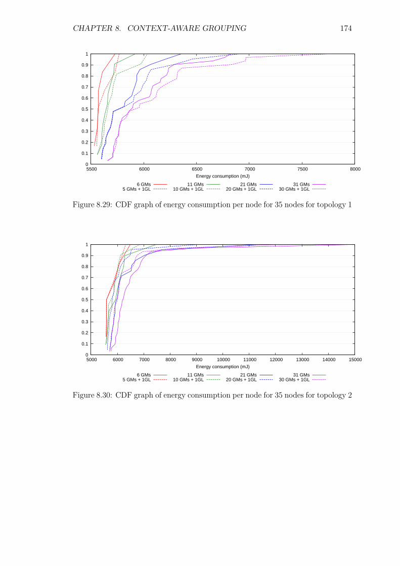
CHAPTER 8. CONTEXT-AWARE GROUPING 174
0
0.1
0.2
0.3
0.4
0.5
0.6
0.7
0.8
0.9
1
5500 6000 6500 7000 7500 8000
Energy consumption (mJ)
6 GMs5 GMs + 1GL
11 GMs10 GMs + 1GL
21 GMs20 GMs + 1GL
31 GMs30 GMs + 1GL
Figure 8.29: CDF graph of energy consumption per node for 35 nodes for topology 1
0
0.1
0.2
0.3
0.4
0.5
0.6
0.7
0.8
0.9
1
5000 6000 7000 8000 9000 10000 11000 12000 13000 14000 15000
Energy consumption (mJ)
6 GMs5 GMs + 1GL
11 GMs10 GMs + 1GL
21 GMs20 GMs + 1GL
31 GMs30 GMs + 1GL
Figure 8.30: CDF graph of energy consumption per node for 35 nodes for topology 2
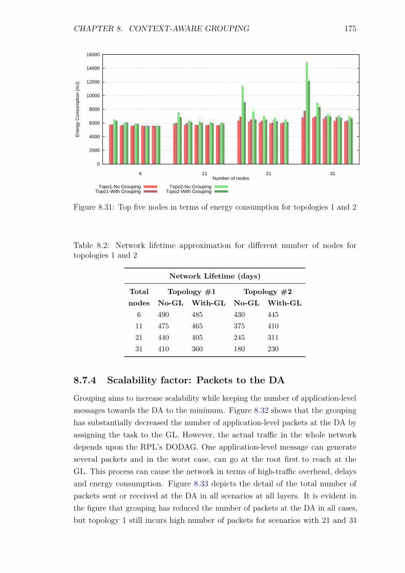
CHAPTER 8. CONTEXT-AWARE GROUPING 175
0
2000
4000
6000
8000
10000
12000
14000
16000
Ene
rgy
Con
sum
ptio
n (m
J)
Number of nodes
Topo1-No GroupingTopo1-With Grouping
Topo2-No GroupingTopo2-With Grouping
3121116
Figure 8.31: Top five nodes in terms of energy consumption for topologies 1 and 2
Table 8.2: Network lifetime approximation for different number of nodes fortopologies 1 and 2
Network Lifetime (days)
Total Topology #1 Topology #2nodes No-GL With-GL No-GL With-GL
6 490 485 430 44511 475 465 375 41021 440 405 245 31131 410 360 180 230
8.7.4 Scalability factor: Packets to the DA
Grouping aims to increase scalability while keeping the number of application-levelmessages towards the DA to the minimum. Figure 8.32 shows that the groupinghas substantially decreased the number of application-level packets at the DA byassigning the task to the GL. However, the actual traffic in the whole networkdepends upon the RPL’s DODAG. One application-level message can generateseveral packets and in the worst case, can go at the root first to reach at theGL. This process can cause the network in terms of high-traffic overhead, delaysand energy consumption. Figure 8.33 depicts the detail of the total number ofpackets sent or received at the DA in all scenarios at all layers. It is evident inthe figure that grouping has reduced the number of packets at the DA in all cases,but topology 1 still incurs high number of packets for scenarios with 21 and 31
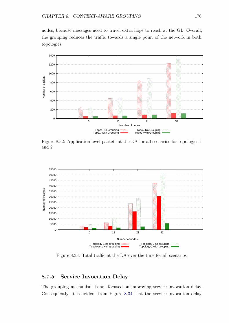
CHAPTER 8. CONTEXT-AWARE GROUPING 176
nodes, because messages need to travel extra hops to reach at the GL. Overall,the grouping reduces the traffic towards a single point of the network in bothtopologies.
0
200
400
600
800
1000
1200
1400
6 11 21 31
Num
ber
of p
acke
ts
Number of nodes
Topo1-No GroupingTopo1-With Grouping
Topo2-No GroupingTopo2-With Grouping
Figure 8.32: Application-level packets at the DA for all scenarios for topologies 1and 2
0
5000
10000
15000
20000
25000
30000
35000
40000
45000
50000
55000
6 11 21 31
Num
ber
of P
acke
ts
Number of nodes
Topology-1 no groupingTopology-1 with grouping
Topology-2 no groupingTopology-2 with grouping
Figure 8.33: Total traffic at the DA over the time for all scenarios
8.7.5 Service Invocation Delay
The grouping mechanism is not focused on improving service invocation delay.Consequently, it is evident from Figure 8.34 that the service invocation delay
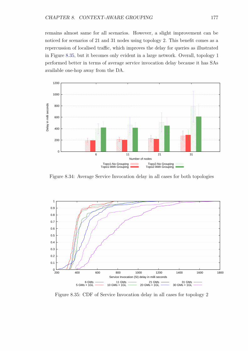
CHAPTER 8. CONTEXT-AWARE GROUPING 177
remains almost same for all scenarios. However, a slight improvement can benoticed for scenarios of 21 and 31 nodes using topology 2. This benefit comes as arepercussion of localised traffic, which improves the delay for queries as illustratedin Figure 8.35, but it becomes only evident in a large network. Overall, topology 1performed better in terms of average service invocation delay because it has SAsavailable one-hop away from the DA.
0
200
400
600
800
1000
1200
6 11 21 31
Del
ay in
mill
i sec
onds
Number of nodes
Topo1-No GroupingTopo1-With Grouping
Topo2-No GroupingTopo2-With Grouping
Figure 8.34: Average Service Invocation delay in all cases for both topologies
0
0.1
0.2
0.3
0.4
0.5
0.6
0.7
0.8
0.9
1
200 400 600 800 1000 1200 1400 1600 1800
Service Invocation (SI) delay in milli seconds
6 GMs5 GMs + 1GL
11 GMs10 GMs + 1GL
21 GMs20 GMs + 1GL
31 GMs30 GMs + 1GL
Figure 8.35: CDF of Service Invocation delay in all cases for topology 2
CHAPTER 8. CONTEXT-AWARE GROUPING 178
8.7.6 Reliability and Accuracy
Grouping makes the GL responsible for informing about the missing nodes, sochance of obsolete registry entries is eliminated. In experiments all service invoc-ation requests and responses are validated and were found accurate, so all thecommunicated information was correct and reliable.
8.8 Experiments: Grouping with differentgroups
This section covers the detail of experiments, including scenarios, experimentalset-up and discussion of the results performed to evaluate the impact of groupingand creation of multiple groups in networks with different topologies.
8.8.1 Introduction
The scalability testing of grouping is done in Section 8.7 where experiments weredone only for one group of nodes with a GL. This section scrutinise the groupingmechanism further by increasing the number of groups in different topologies.Following scenarios are used in experiments.
Case 1 - Basic TRENDY without grouping: This scenario only enables thebasic functionality of the proposed solution where a UA gets a single bestmatched service information.
Case 2 - Basic TRENDY with 5 GL: This case has grouping mechanism en-abled with 5 GLs that are placed one in each of the 5 locations, on top ofcase 1’s functionality. In all topologies, node 2-6 (No. 1 is the border router)were assigned the role of GLs for their groups.
Case 3- GL failure scenario with 6 GLs: This scenario has 6 GLs (node 12as well), where one of them fails during the simulation (after 1000 seconds)and other GL is reselected by the DA. All topologies are same like case 2, buttopology 1 is slightly changed for this case and position of node 2 is swappedwith node 7 to maintain the DODAG tree after the GL’s failure.
The simulations were configured with the same settings defined in Section 6.3with the changes given in Table 8.3. In the case of TRENDY with grouping, onephysical topology translates into three different topologies: physical topology, RPLtopology and application-level trendy tree topology formed after grouping. Theexperiments for the above scenarios are conducted using three physical topologies
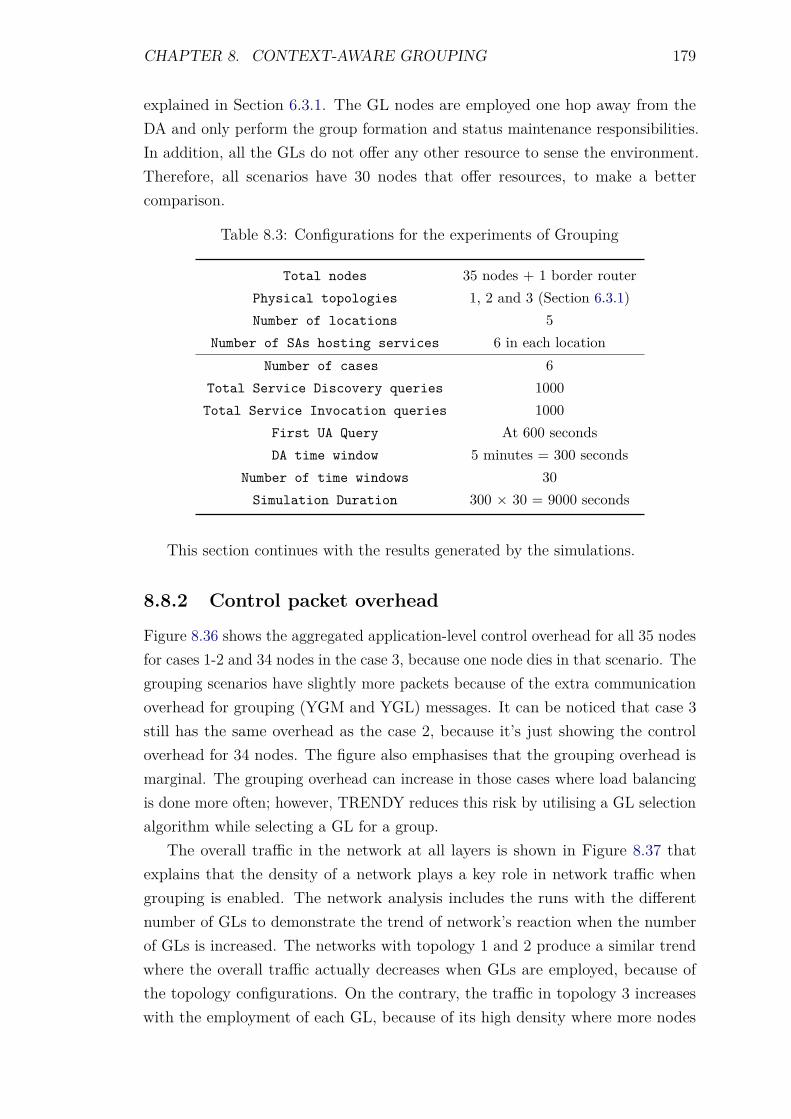
CHAPTER 8. CONTEXT-AWARE GROUPING 179
explained in Section 6.3.1. The GL nodes are employed one hop away from theDA and only perform the group formation and status maintenance responsibilities.In addition, all the GLs do not offer any other resource to sense the environment.Therefore, all scenarios have 30 nodes that offer resources, to make a bettercomparison.
Table 8.3: Configurations for the experiments of Grouping
Total nodes 35 nodes + 1 border routerPhysical topologies 1, 2 and 3 (Section 6.3.1)Number of locations 5
Number of SAs hosting services 6 in each locationNumber of cases 6
Total Service Discovery queries 1000Total Service Invocation queries 1000
First UA Query At 600 secondsDA time window 5 minutes = 300 seconds
Number of time windows 30Simulation Duration 300 × 30 = 9000 seconds
This section continues with the results generated by the simulations.
8.8.2 Control packet overhead
Figure 8.36 shows the aggregated application-level control overhead for all 35 nodesfor cases 1-2 and 34 nodes in the case 3, because one node dies in that scenario. Thegrouping scenarios have slightly more packets because of the extra communicationoverhead for grouping (YGM and YGL) messages. It can be noticed that case 3still has the same overhead as the case 2, because it’s just showing the controloverhead for 34 nodes. The figure also emphasises that the grouping overhead ismarginal. The grouping overhead can increase in those cases where load balancingis done more often; however, TRENDY reduces this risk by utilising a GL selectionalgorithm while selecting a GL for a group.
The overall traffic in the network at all layers is shown in Figure 8.37 thatexplains that the density of a network plays a key role in network traffic whengrouping is enabled. The network analysis includes the runs with the differentnumber of GLs to demonstrate the trend of network’s reaction when the numberof GLs is increased. The networks with topology 1 and 2 produce a similar trendwhere the overall traffic actually decreases when GLs are employed, because ofthe topology configurations. On the contrary, the traffic in topology 3 increaseswith the employment of each GL, because of its high density where more nodes
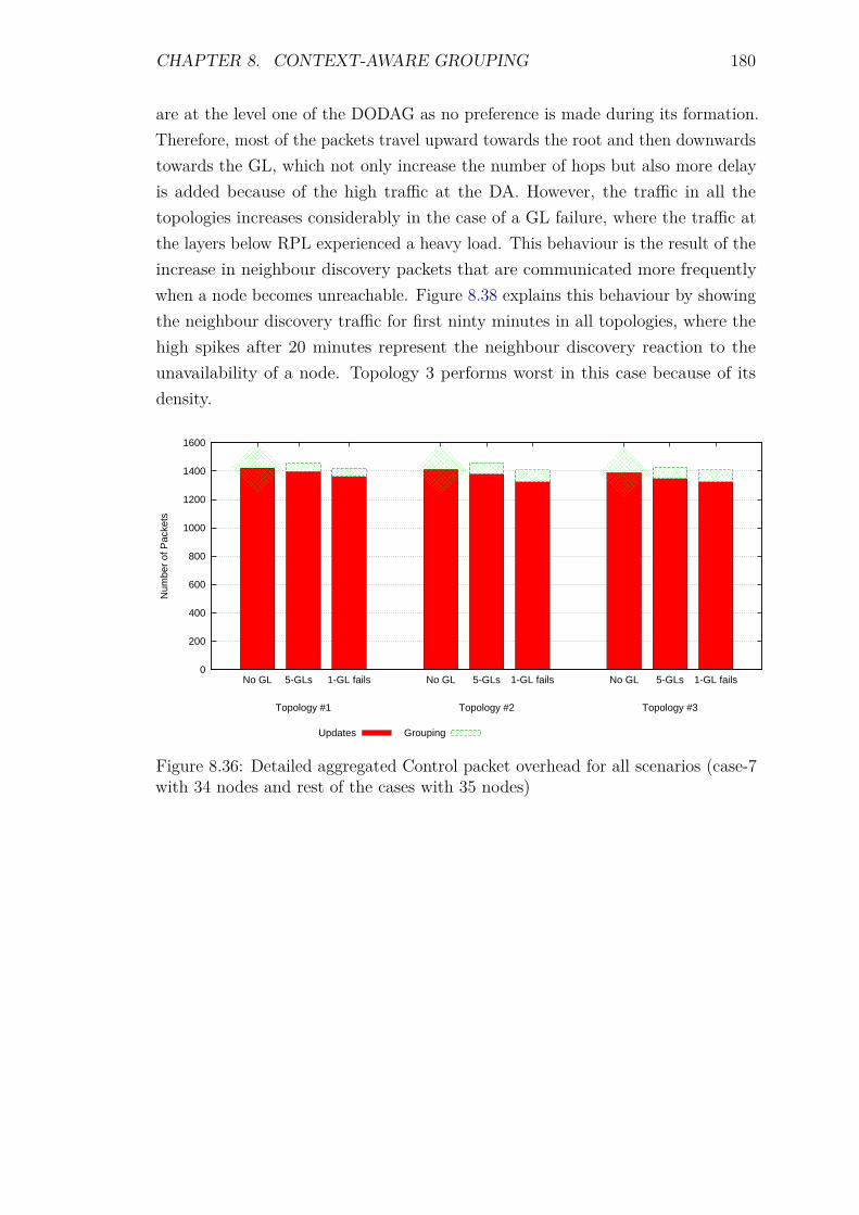
CHAPTER 8. CONTEXT-AWARE GROUPING 180
are at the level one of the DODAG as no preference is made during its formation.Therefore, most of the packets travel upward towards the root and then downwardstowards the GL, which not only increase the number of hops but also more delayis added because of the high traffic at the DA. However, the traffic in all thetopologies increases considerably in the case of a GL failure, where the traffic atthe layers below RPL experienced a heavy load. This behaviour is the result of theincrease in neighbour discovery packets that are communicated more frequentlywhen a node becomes unreachable. Figure 8.38 explains this behaviour by showingthe neighbour discovery traffic for first ninty minutes in all topologies, where thehigh spikes after 20 minutes represent the neighbour discovery reaction to theunavailability of a node. Topology 3 performs worst in this case because of itsdensity.
0
200
400
600
800
1000
1200
1400
1600
No GL 5-GLs 1-GL fails No GL 5-GLs 1-GL fails No GL 5-GLs 1-GL fails
Num
ber
of P
acke
ts
Updates Grouping
Topology #3Topology #2Topology #1
Figure 8.36: Detailed aggregated Control packet overhead for all scenarios (case-7with 34 nodes and rest of the cases with 35 nodes)
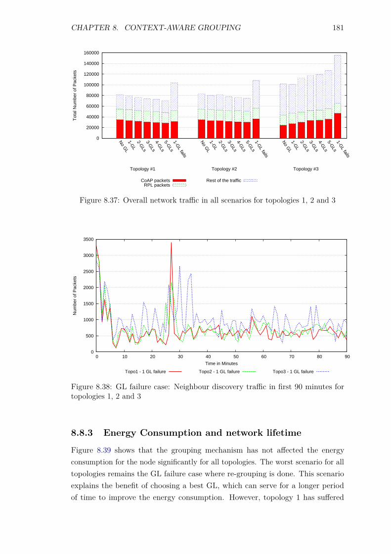
CHAPTER 8. CONTEXT-AWARE GROUPING 181
0
20000
40000
60000
80000
100000
120000
140000
160000
No G
L1-G
L2-G
Ls3-G
Ls4-G
Ls5-G
Ls1-G
L fails
No G
L1-G
L2-G
Ls3-G
Ls4-G
Ls5-G
Ls1-G
L fails
No G
L1-G
L2-G
Ls3-G
Ls4-G
Ls5-G
Ls1-G
L fails
Tot
al N
umbe
r of
Pac
kets
CoAP packetsRPL packets
Rest of the traffic
Topology #3Topology #2Topology #1
Figure 8.37: Overall network traffic in all scenarios for topologies 1, 2 and 3
0
500
1000
1500
2000
2500
3000
3500
0 10 20 30 40 50 60 70 80 90
Num
ber
of P
acke
ts
Time in Minutes
Topo1 - 1 GL failure Topo2 - 1 GL failure Topo3 - 1 GL failure
Figure 8.38: GL failure case: Neighbour discovery traffic in first 90 minutes fortopologies 1, 2 and 3
8.8.3 Energy Consumption and network lifetime
Figure 8.39 shows that the grouping mechanism has not affected the energyconsumption for the node significantly for all topologies. The worst scenario for alltopologies remains the GL failure case where re-grouping is done. This scenarioexplains the benefit of choosing a best GL, which can serve for a longer periodof time to improve the energy consumption. However, topology 1 has suffered
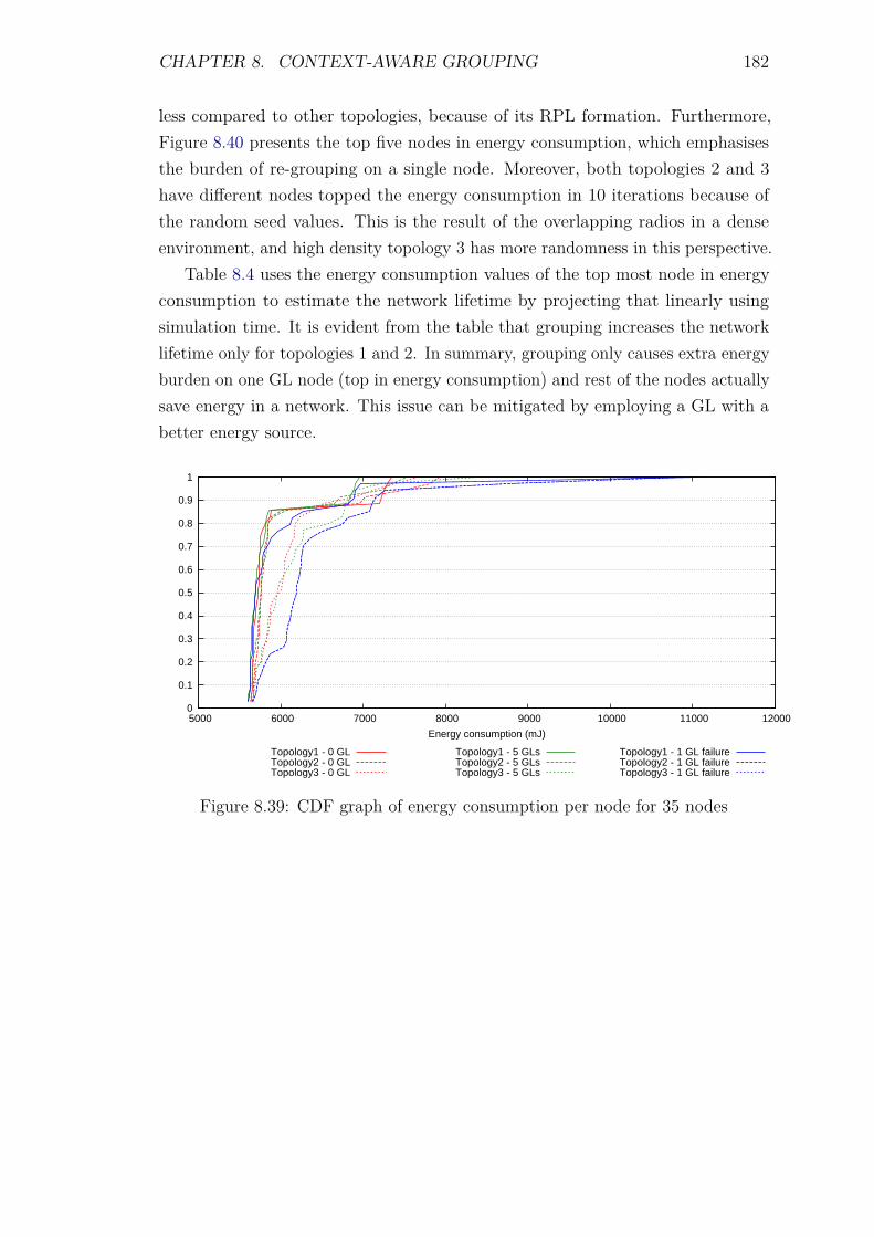
CHAPTER 8. CONTEXT-AWARE GROUPING 182
less compared to other topologies, because of its RPL formation. Furthermore,Figure 8.40 presents the top five nodes in energy consumption, which emphasisesthe burden of re-grouping on a single node. Moreover, both topologies 2 and 3have different nodes topped the energy consumption in 10 iterations because ofthe random seed values. This is the result of the overlapping radios in a denseenvironment, and high density topology 3 has more randomness in this perspective.
Table 8.4 uses the energy consumption values of the top most node in energyconsumption to estimate the network lifetime by projecting that linearly usingsimulation time. It is evident from the table that grouping increases the networklifetime only for topologies 1 and 2. In summary, grouping only causes extra energyburden on one GL node (top in energy consumption) and rest of the nodes actuallysave energy in a network. This issue can be mitigated by employing a GL with abetter energy source.
0
0.1
0.2
0.3
0.4
0.5
0.6
0.7
0.8
0.9
1
5000 6000 7000 8000 9000 10000 11000 12000
Energy consumption (mJ)
Topology1 - 0 GLTopology2 - 0 GLTopology3 - 0 GL
Topology1 - 5 GLsTopology2 - 5 GLsTopology3 - 5 GLs
Topology1 - 1 GL failureTopology2 - 1 GL failureTopology3 - 1 GL failure
Figure 8.39: CDF graph of energy consumption per node for 35 nodes
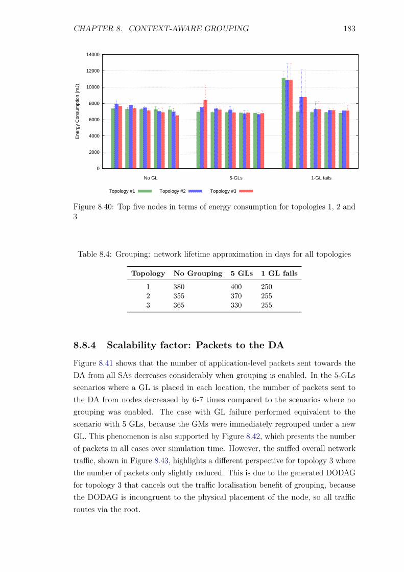
CHAPTER 8. CONTEXT-AWARE GROUPING 183
0
2000
4000
6000
8000
10000
12000
14000
Ene
rgy
Con
sum
ptio
n (m
J)
Topology #1 Topology #2 Topology #3
1-GL fails5-GLsNo GL
Figure 8.40: Top five nodes in terms of energy consumption for topologies 1, 2 and3
Table 8.4: Grouping: network lifetime approximation in days for all topologies
Topology No Grouping 5 GLs 1 GL fails
1 380 400 2502 355 370 2553 365 330 255
8.8.4 Scalability factor: Packets to the DA
Figure 8.41 shows that the number of application-level packets sent towards theDA from all SAs decreases considerably when grouping is enabled. In the 5-GLsscenarios where a GL is placed in each location, the number of packets sent tothe DA from nodes decreased by 6-7 times compared to the scenarios where nogrouping was enabled. The case with GL failure performed equivalent to thescenario with 5 GLs, because the GMs were immediately regrouped under a newGL. This phenomenon is also supported by Figure 8.42, which presents the numberof packets in all cases over simulation time. However, the sniffed overall networktraffic, shown in Figure 8.43, highlights a different perspective for topology 3 wherethe number of packets only slightly reduced. This is due to the generated DODAGfor topology 3 that cancels out the traffic localisation benefit of grouping, becausethe DODAG is incongruent to the physical placement of the node, so all trafficroutes via the root.
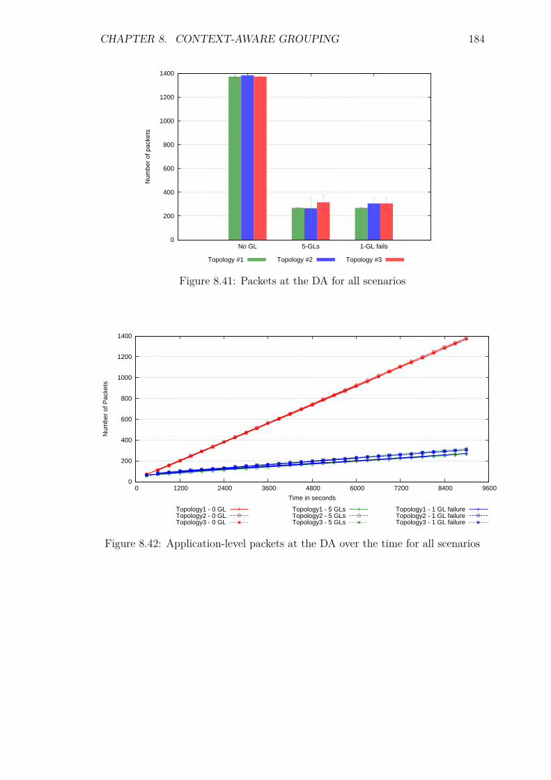
CHAPTER 8. CONTEXT-AWARE GROUPING 184
0
200
400
600
800
1000
1200
1400
No GL 5-GLs 1-GL fails
Num
ber
of p
acke
ts
Topology #1 Topology #2 Topology #3
Figure 8.41: Packets at the DA for all scenarios
0
200
400
600
800
1000
1200
1400
0 1200 2400 3600 4800 6000 7200 8400 9600
Num
ber
of P
acke
ts
Time in seconds
Topology1 - 0 GLTopology2 - 0 GLTopology3 - 0 GL
Topology1 - 5 GLsTopology2 - 5 GLsTopology3 - 5 GLs
Topology1 - 1 GL failureTopology2 - 1 GL failureTopology3 - 1 GL failure
Figure 8.42: Application-level packets at the DA over the time for all scenarios
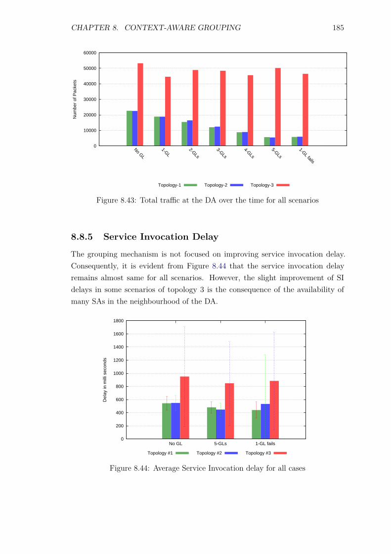
CHAPTER 8. CONTEXT-AWARE GROUPING 185
0
10000
20000
30000
40000
50000
60000
No GL
1-GL2-GLs
3-GLs
4-GLs
5-GLs
1-GL fails
Num
ber
of P
acke
ts
Topology-1 Topology-2 Topology-3
Figure 8.43: Total traffic at the DA over the time for all scenarios
8.8.5 Service Invocation Delay
The grouping mechanism is not focused on improving service invocation delay.Consequently, it is evident from Figure 8.44 that the service invocation delayremains almost same for all scenarios. However, the slight improvement of SIdelays in some scenarios of topology 3 is the consequence of the availability ofmany SAs in the neighbourhood of the DA.
0
200
400
600
800
1000
1200
1400
1600
1800
No GL 5-GLs 1-GL fails
Del
ay in
mill
i sec
onds
Topology #1 Topology #2 Topology #3
Figure 8.44: Average Service Invocation delay for all cases
CHAPTER 8. CONTEXT-AWARE GROUPING 186
8.8.6 Reliability and Accuracy
Grouping distributes the status maintenance task by allocating GLs in differentareas of a network. The GLs report to the DA regarding each unresponsive SAto ensure the accuracy of service information maintained at the DA. All serviceinvocation responses are validated and found successful that explains that the DAprovided accurate information to all SD requests.
8.9 Summary and Discussion
This chapter covered the detail of a context-aware grouping mechanism thatlocalises status maintenance traffic and enables a paradigm for service compositionto facilitate the future WoT applications. Furthermore, it eradicates the bottleneckproblem associated with a centralised directory and makes a network more scalable,by localising the status maintenance traffic. It also devises modular profiles formore capable devices to gain benefits of distribution of jobs. The idea of groupingbecomes useful when less load balancing is needed, which can be ensured by utilisingproposed GL selection algorithm.
The scalability of grouping is evaluated in simulations by varying the size ofa group, and it is found that grouping improves the control overehead, energyefficiency and total DA traffic for all cases in topologies with different densities.However, it is also found that the energy consumption and total traffic of a networkdepend on the RPL’s DODAG and the number of direct neighbours of a node.Therefore, it increases the energy consumption of the nodes when the congruencybetween grouping topology and DODAG increases, which is common in a networkwith high node density. The scrutiny of grouping mechanism in a network offew groups is also done, which emphasises the role of network’s density on totaltraffic and energy consumption of the network. It is also concluded from theexperiments that if a GL fails during the lifetime of the network, the load balancingwill increase the overhead, and the newly selected GL pays the price in form ofenergy consumption. Therefore, the role of the GL selection algorithm becomesimportant to reduce the probability of a GL failure by selecting a wise choice duringthe GL selection. In summary, all the results prove that the grouping mechanismconsiderably reduces the number of packets towards the DA and improves theenergy efficiency and network lifetime while marginally increasing the controloverhead.
The next chapter covers the detail of the proposed adaptive caching mechanism.
Chapter 9
Adaptive Piggybacked Publishing(APPUB): An Algorithm forAdaptive Caching
9.1 Introduction
Chapters 5, 7 and 8 covered the details of the proposed context-aware SDP, adapt-ive timer and grouping mechanisms, respectively. However, only service selectionmechanism addresses the service invocation delay to improve user response. Thischapter focuses on improving the service invocation delay by offering adaptive cach-ing mechanism. Moreover, the adaptability requirement (Section 4.4.3) demandsa technique that can adaptively arrange cached values for user applications. Inaddition, the high number of service invocations increases the traffic and energyconsumption for nodes in a multi-hop network by keeping them awake most ofthe time. Furthermore, the constraints of involved devices can restrict them to beavailable more frequently, as these are prone to failure because of depleted batteries.Therefore, the effect of the high number of service invocations will decrease thenetwork lifetime. This chapter proposes a technique that arranges cache values bysensing the popularity of services.
9.2 Aims
The aims for the required adaptive caching technique are:
1. The process of maintaining cache values should have low control overhead.
2. The algorithm should be adaptive to a context-aware criteria, e.g., demandof services, so that criteria should be checked first before making the decision
187
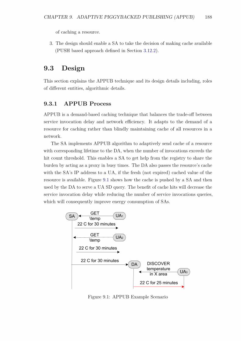
CHAPTER 9. ADAPTIVE PIGGYBACKED PUBLISHING (APPUB) 188
of caching a resource.
3. The design should enable a SA to take the decision of making cache available(PUSH based approach defined in Section 3.12.2).
9.3 Design
This section explains the APPUB technique and its design details including, rolesof different entities, algorithmic details.
9.3.1 APPUB Process
APPUB is a demand-based caching technique that balances the trade-off betweenservice invocation delay and network efficiency. It adapts to the demand of aresource for caching rather than blindly maintaining cache of all resources in anetwork.
The SA implements APPUB algorithm to adaptively send cache of a resourcewith corresponding lifetime to the DA, when the number of invocations exceeds thehit count threshold. This enables a SA to get help from the registry to share theburden by acting as a proxy in busy times. The DA also passes the resource’s cachewith the SA’s IP address to a UA, if the fresh (not expired) cached value of theresource is available. Figure 9.1 shows how the cache is pushed by a SA and thenused by the DA to serve a UA SD query. The benefit of cache hits will decrease theservice invocation delay while reducing the number of service invocations queries,which will consequently improve energy consumption of SAs.
�����
���
�� � �� � � �������
��������
��������
��
����������������� � � ���
�� � �� � � �����
�� � �� � � �����
�� � �� � � �����
Figure 9.1: APPUB Example Scenario
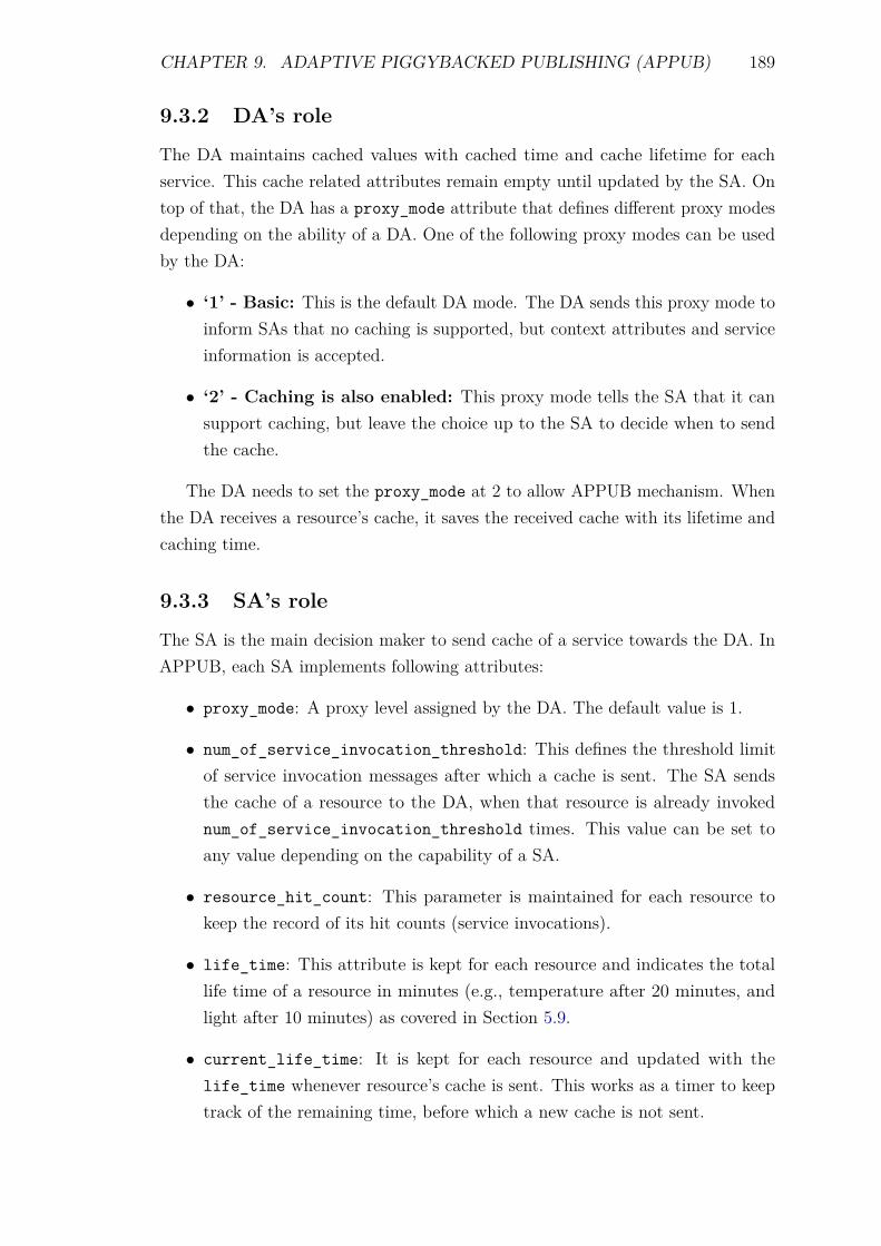
CHAPTER 9. ADAPTIVE PIGGYBACKED PUBLISHING (APPUB) 189
9.3.2 DA’s role
The DA maintains cached values with cached time and cache lifetime for eachservice. This cache related attributes remain empty until updated by the SA. Ontop of that, the DA has a proxy_mode attribute that defines different proxy modesdepending on the ability of a DA. One of the following proxy modes can be usedby the DA:
• ‘1’ - Basic: This is the default DA mode. The DA sends this proxy mode toinform SAs that no caching is supported, but context attributes and serviceinformation is accepted.
• ‘2’ - Caching is also enabled: This proxy mode tells the SA that it cansupport caching, but leave the choice up to the SA to decide when to sendthe cache.
The DA needs to set the proxy_mode at 2 to allow APPUB mechanism. Whenthe DA receives a resource’s cache, it saves the received cache with its lifetime andcaching time.
9.3.3 SA’s role
The SA is the main decision maker to send cache of a service towards the DA. InAPPUB, each SA implements following attributes:
• proxy_mode: A proxy level assigned by the DA. The default value is 1.
• num_of_service_invocation_threshold: This defines the threshold limitof service invocation messages after which a cache is sent. The SA sendsthe cache of a resource to the DA, when that resource is already invokednum_of_service_invocation_threshold times. This value can be set toany value depending on the capability of a SA.
• resource_hit_count: This parameter is maintained for each resource tokeep the record of its hit counts (service invocations).
• life_time: This attribute is kept for each resource and indicates the totallife time of a resource in minutes (e.g., temperature after 20 minutes, andlight after 10 minutes) as covered in Section 5.9.
• current_life_time: It is kept for each resource and updated with thelife_time whenever resource’s cache is sent. This works as a timer to keeptrack of the remaining time, before which a new cache is not sent.
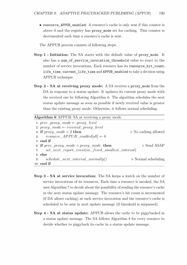
CHAPTER 9. ADAPTIVE PIGGYBACKED PUBLISHING (APPUB) 190
• resource_APPUB_enabled: A resource’s cache is only sent if this counter isabove 0 and the registry has proxy_mode set for caching. This counter isdecremented each time a resource’s cache is sent.
The APPUB process consists of following steps:
Step 1 - Initiation: The SA starts with the default value of proxy_mode. Italso has a num_of_service_invocation_threshold value to react to thenumber of service invocations. Each resource has its resource_hit_count,life_time, current_life_time and APPUB_enabled to take a decision usingAPPUB technique.
Step 2 - SA at receiving proxy mode: A SA receives a proxy_mode from theDA in response to a status update. It updates its current proxy mode withthe received one by following Algorithm 6. The algorithm schedules the nextstatus update message as soon as possible if newly received value is greaterthan the existing proxy mode. Otherwise, it follows normal scheduling.
Algorithm 6 APPUB: SA at receiving a proxy mode1: prev_proxy_mode← proxy_level2: proxy_mode← received_proxy_level3: if proxy_mode < 2 then . No caching allowed4: resource_APPUB_enabled[all]← 05: end if6: if prev_proxy_mode < proxy_mode then . Send ASAP7: set_next_report_event(in_fixed_smallest_interval)8: else9: schedule_next_interval_normally() . Normal scheduling10: end if
Step 3 - SA at service invocation: The SA keeps a watch on the number ofservice invocations of its resources. Each time a resource is invoked, the SAuses Algorithm 7 to decide about the possibility of sending the resource’s cachein the next status update message. The resource’s hit count is incremented(if DA allows caching) at each service invocation and the resource’s cache isscheduled to be sent in next update message (if threshold is surpassed).
Step 4 - SA at status update: APPUB allows the cache to be piggybacked ina status update message. The SA follows Algorithm 8 for every resource todecide whether to piggyback its cache in a status update message.
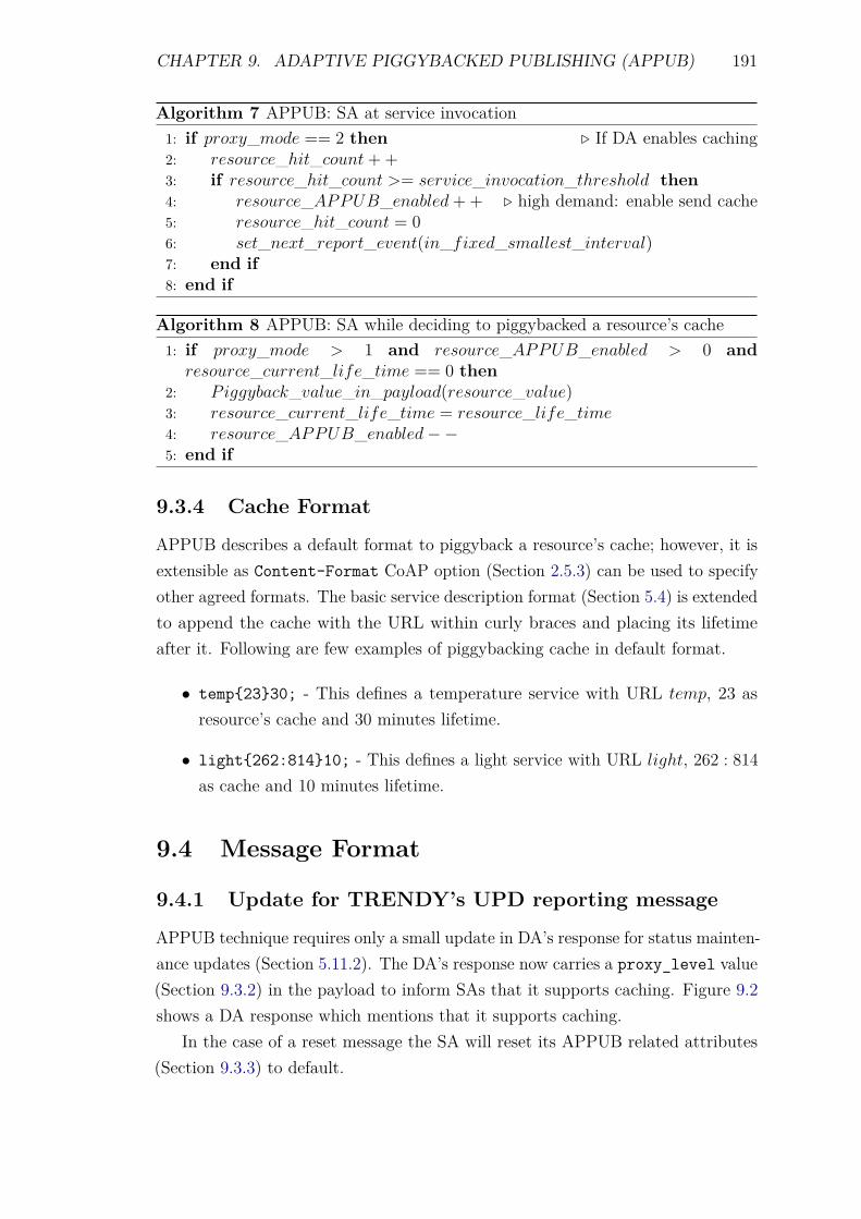
CHAPTER 9. ADAPTIVE PIGGYBACKED PUBLISHING (APPUB) 191
Algorithm 7 APPUB: SA at service invocation1: if proxy_mode == 2 then . If DA enables caching2: resource_hit_count + +3: if resource_hit_count >= service_invocation_threshold then4: resource_APPUB_enabled + + . high demand: enable send cache5: resource_hit_count = 06: set_next_report_event(in_fixed_smallest_interval)7: end if8: end if
Algorithm 8 APPUB: SA while deciding to piggybacked a resource’s cache1: if proxy_mode > 1 and resource_APPUB_enabled > 0 and
resource_current_life_time == 0 then2: Piggyback_value_in_payload(resource_value)3: resource_current_life_time = resource_life_time4: resource_APPUB_enabled−−5: end if
9.3.4 Cache Format
APPUB describes a default format to piggyback a resource’s cache; however, it isextensible as Content-Format CoAP option (Section 2.5.3) can be used to specifyother agreed formats. The basic service description format (Section 5.4) is extendedto append the cache with the URL within curly braces and placing its lifetimeafter it. Following are few examples of piggybacking cache in default format.
• temp{23}30; - This defines a temperature service with URL temp, 23 asresource’s cache and 30 minutes lifetime.
• light{262:814}10; - This defines a light service with URL light, 262 : 814as cache and 10 minutes lifetime.
9.4 Message Format
9.4.1 Update for TRENDY’s UPD reporting message
APPUB technique requires only a small update in DA’s response for status mainten-ance updates (Section 5.11.2). The DA’s response now carries a proxy_level value(Section 9.3.2) in the payload to inform SAs that it supports caching. Figure 9.2shows a DA response which mentions that it supports caching.
In the case of a reset message the SA will reset its APPUB related attributes(Section 9.3.3) to default.
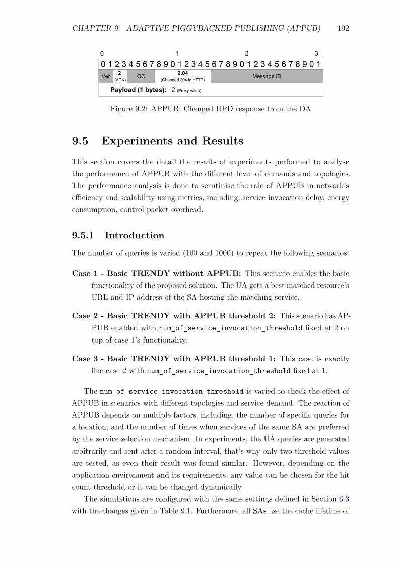
CHAPTER 9. ADAPTIVE PIGGYBACKED PUBLISHING (APPUB) 192
� � � � � � � � � � � � � � � � � � � � � � � � � ��� ��
������� �� ��� � � �� ��� ������
� � � �
������
��������� �! ��� "� #$$��
%�&&� � '(
Figure 9.2: APPUB: Changed UPD response from the DA
9.5 Experiments and Results
This section covers the detail the results of experiments performed to analysethe performance of APPUB with the different level of demands and topologies.The performance analysis is done to scrutinise the role of APPUB in network’sefficiency and scalability using metrics, including, service invocation delay, energyconsumption, control packet overhead.
9.5.1 Introduction
The number of queries is varied (100 and 1000) to repeat the following scenarios:
Case 1 - Basic TRENDY without APPUB: This scenario enables the basicfunctionality of the proposed solution. The UA gets a best matched resource’sURL and IP address of the SA hosting the matching service.
Case 2 - Basic TRENDY with APPUB threshold 2: This scenario has AP-PUB enabled with num_of_service_invocation_threshold fixed at 2 ontop of case 1’s functionality.
Case 3 - Basic TRENDY with APPUB threshold 1: This case is exactlylike case 2 with num_of_service_invocation_threshold fixed at 1.
The num_of_service_invocation_threshold is varied to check the effect ofAPPUB in scenarios with different topologies and service demand. The reaction ofAPPUB depends on multiple factors, including, the number of specific queries fora location, and the number of times when services of the same SA are preferredby the service selection mechanism. In experiments, the UA queries are generatedarbitrarily and sent after a random interval, that’s why only two threshold valuesare tested, as even their result was found similar. However, depending on theapplication environment and its requirements, any value can be chosen for the hitcount threshold or it can be changed dynamically.
The simulations are configured with the same settings defined in Section 6.3with the changes given in Table 9.1. Furthermore, all SAs use the cache lifetime of

CHAPTER 9. ADAPTIVE PIGGYBACKED PUBLISHING (APPUB) 193
10, 30 and 60 minutes for light, temperature and humidity resources, respectively.These cache lifetimes were selected randomly and have no impact on the querygeneration process.
Table 9.1: Configurations for the experiments of APPUB
Total nodes 35 nodes + 1 border routerPhysical topologies 1, 2 and 3 (Section 6.3.1)
RDC ContikiMAC and NullRDCNumber of locations 5 with 7 SAs in each location
Total Service Discovery queries 100 and 1000Total Service Invocation queries 100 and 1000
Number of cases 3 (cases)× 2 (query variations) = 6First UA Query At 600 secondsDA time window 5 minutes = 300 seconds
Number of time windows 30Simulation Duration 300 × 30 = 9000 seconds
This section continues with the generated results of simulations to analyse theeffect of the APPUB mechanism.
9.5.2 Service Invocation Delay and Cache hits
The APPUB mechanism adaptively makes cached values available at the DA, whichare then used to serve future queries to decrease the overall service invocation delayand overhead incur while passing a message over a multi-hop network. Figure 9.3shows the number of cache hits (the number of times maintained cache is used) inall cases. Both APPUB cases have served 60 − 70% of UA queries with cachedvalues regardless of the employed RDC. There is no significant difference betweencase 2 and 3, because of the randomness introduced by query generation process,and service selection’s preference for choosing a SA to serve a query. Furthermore,the figure shows a contradiction where more sensitive hit-count threshold valueactually proved less efficient in some scenarios. However, the scenarios with smallthreshold value show better performance in the cases of 100 queries, because ofthe randomness in the query generation and arrival process.
Figure 9.4 demonstrates the impact of APPUB for first 100 UA queries inscenarios with 1000 queries using ContikiMAC. It is evident that the DA startedserving the queries with cache values after first 40 randomly generated queries.This reaction comes from the adaptive nature of APPUB that senses the highnumber of queries and arranges cache at the DA. Furthermore, the small hit countthreshold value reacted to the load quickly to serve the query with a cached value
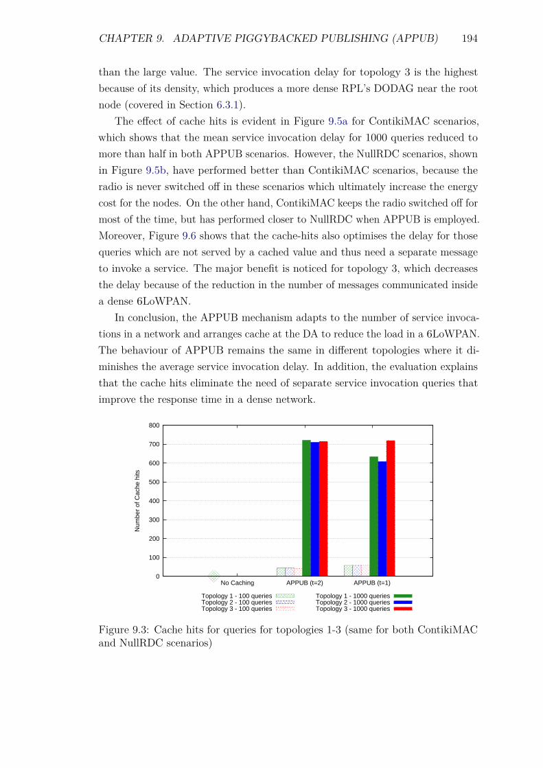
CHAPTER 9. ADAPTIVE PIGGYBACKED PUBLISHING (APPUB) 194
than the large value. The service invocation delay for topology 3 is the highestbecause of its density, which produces a more dense RPL’s DODAG near the rootnode (covered in Section 6.3.1).
The effect of cache hits is evident in Figure 9.5a for ContikiMAC scenarios,which shows that the mean service invocation delay for 1000 queries reduced tomore than half in both APPUB scenarios. However, the NullRDC scenarios, shownin Figure 9.5b, have performed better than ContikiMAC scenarios, because theradio is never switched off in these scenarios which ultimately increase the energycost for the nodes. On the other hand, ContikiMAC keeps the radio switched off formost of the time, but has performed closer to NullRDC when APPUB is employed.Moreover, Figure 9.6 shows that the cache-hits also optimises the delay for thosequeries which are not served by a cached value and thus need a separate messageto invoke a service. The major benefit is noticed for topology 3, which decreasesthe delay because of the reduction in the number of messages communicated insidea dense 6LoWPAN.
In conclusion, the APPUB mechanism adapts to the number of service invoca-tions in a network and arranges cache at the DA to reduce the load in a 6LoWPAN.The behaviour of APPUB remains the same in different topologies where it di-minishes the average service invocation delay. In addition, the evaluation explainsthat the cache hits eliminate the need of separate service invocation queries thatimprove the response time in a dense network.
0
100
200
300
400
500
600
700
800
No Caching APPUB (t=2) APPUB (t=1)
Num
ber
of C
ache
hits
Topology 1 - 100 queriesTopology 2 - 100 queriesTopology 3 - 100 queries
Topology 1 - 1000 queriesTopology 2 - 1000 queriesTopology 3 - 1000 queries
Figure 9.3: Cache hits for queries for topologies 1-3 (same for both ContikiMACand NullRDC scenarios)
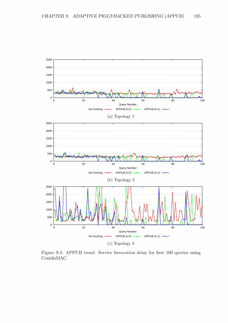
CHAPTER 9. ADAPTIVE PIGGYBACKED PUBLISHING (APPUB) 195
0
500
1000
1500
2000
2500
0 20 40 60 80 100
Query Number
No Caching APPUB (t=2) APPUB (t=1)
(a) Topology 1
0
500
1000
1500
2000
2500
0 20 40 60 80 100
Query Number
No Caching APPUB (t=2) APPUB (t=1)
(b) Topology 2
0
500
1000
1500
2000
2500
0 20 40 60 80 100
Query Number
No Caching APPUB (t=2) APPUB (t=1)
(c) Topology 3
Figure 9.4: APPUB trend: Service Invocation delay for first 100 queries usingContikiMAC
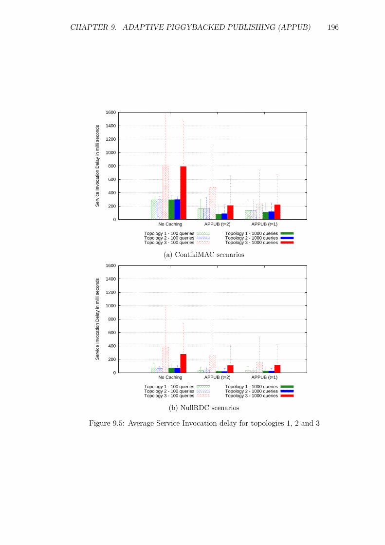
CHAPTER 9. ADAPTIVE PIGGYBACKED PUBLISHING (APPUB) 196
0
200
400
600
800
1000
1200
1400
1600
No Caching APPUB (t=2) APPUB (t=1)
Ser
vice
Invo
catio
n D
elay
in m
illi s
econ
ds
Topology 1 - 100 queriesTopology 2 - 100 queriesTopology 3 - 100 queries
Topology 1 - 1000 queriesTopology 2 - 1000 queriesTopology 3 - 1000 queries
(a) ContikiMAC scenarios
0
200
400
600
800
1000
1200
1400
1600
No Caching APPUB (t=2) APPUB (t=1)
Ser
vice
Invo
catio
n D
elay
in m
illi s
econ
ds
Topology 1 - 100 queriesTopology 2 - 100 queriesTopology 3 - 100 queries
Topology 1 - 1000 queriesTopology 2 - 1000 queriesTopology 3 - 1000 queries
(b) NullRDC scenarios
Figure 9.5: Average Service Invocation delay for topologies 1, 2 and 3
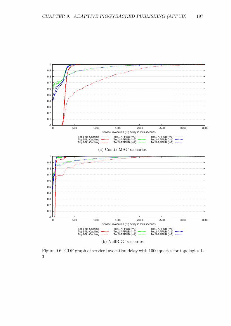
CHAPTER 9. ADAPTIVE PIGGYBACKED PUBLISHING (APPUB) 197
0
0.1
0.2
0.3
0.4
0.5
0.6
0.7
0.8
0.9
1
0 500 1000 1500 2000 2500 3000 3500
Service Invocation (SI) delay in milli seconds
Top1-No CachingTop2-No CachingTop3-No Caching
Top1-APPUB (t=2)Top2-APPUB (t=2)Top3-APPUB (t=2)
Top1-APPUB (t=1)Top2-APPUB (t=1)Top3-APPUB (t=1)
(a) ContikiMAC scenarios
0
0.1
0.2
0.3
0.4
0.5
0.6
0.7
0.8
0.9
1
0 500 1000 1500 2000 2500 3000 3500
Service Invocation (SI) delay in milli seconds
Top1-No CachingTop2-No CachingTop3-No Caching
Top1-APPUB (t=2)Top2-APPUB (t=2)Top3-APPUB (t=2)
Top1-APPUB (t=1)Top2-APPUB (t=1)Top3-APPUB (t=1)
(b) NullRDC scenarios
Figure 9.6: CDF graph of service Invocation delay with 1000 queries for topologies 1-3
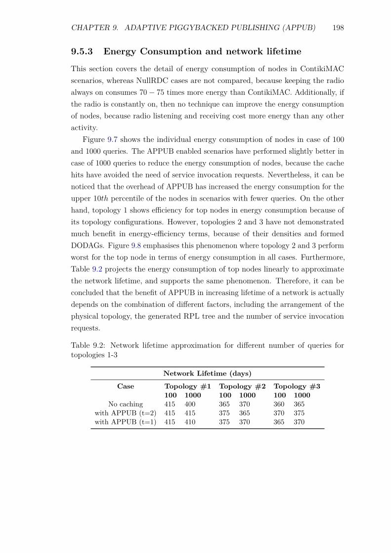
CHAPTER 9. ADAPTIVE PIGGYBACKED PUBLISHING (APPUB) 198
9.5.3 Energy Consumption and network lifetime
This section covers the detail of energy consumption of nodes in ContikiMACscenarios, whereas NullRDC cases are not compared, because keeping the radioalways on consumes 70− 75 times more energy than ContikiMAC. Additionally, ifthe radio is constantly on, then no technique can improve the energy consumptionof nodes, because radio listening and receiving cost more energy than any otheractivity.
Figure 9.7 shows the individual energy consumption of nodes in case of 100and 1000 queries. The APPUB enabled scenarios have performed slightly better incase of 1000 queries to reduce the energy consumption of nodes, because the cachehits have avoided the need of service invocation requests. Nevertheless, it can benoticed that the overhead of APPUB has increased the energy consumption for theupper 10th percentile of the nodes in scenarios with fewer queries. On the otherhand, topology 1 shows efficiency for top nodes in energy consumption because ofits topology configurations. However, topologies 2 and 3 have not demonstratedmuch benefit in energy-efficiency terms, because of their densities and formedDODAGs. Figure 9.8 emphasises this phenomenon where topology 2 and 3 performworst for the top node in terms of energy consumption in all cases. Furthermore,Table 9.2 projects the energy consumption of top nodes linearly to approximatethe network lifetime, and supports the same phenomenon. Therefore, it can beconcluded that the benefit of APPUB in increasing lifetime of a network is actuallydepends on the combination of different factors, including the arrangement of thephysical topology, the generated RPL tree and the number of service invocationrequests.
Table 9.2: Network lifetime approximation for different number of queries fortopologies 1-3
Network Lifetime (days)
Case Topology #1 Topology #2 Topology #3100 1000 100 1000 100 1000
No caching 415 400 365 370 360 365with APPUB (t=2) 415 415 375 365 370 375with APPUB (t=1) 415 410 375 370 365 370
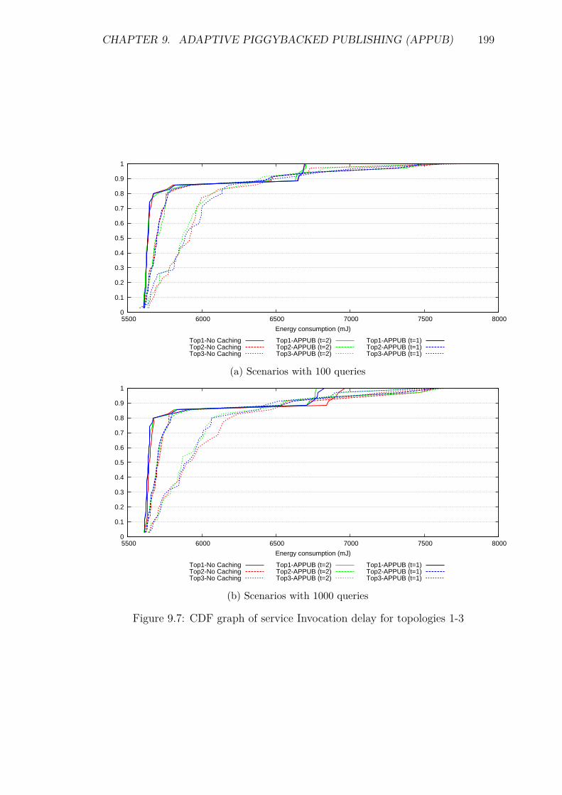
CHAPTER 9. ADAPTIVE PIGGYBACKED PUBLISHING (APPUB) 199
0
0.1
0.2
0.3
0.4
0.5
0.6
0.7
0.8
0.9
1
5500 6000 6500 7000 7500 8000
Energy consumption (mJ)
Top1-No CachingTop2-No CachingTop3-No Caching
Top1-APPUB (t=2)Top2-APPUB (t=2)Top3-APPUB (t=2)
Top1-APPUB (t=1)Top2-APPUB (t=1)Top3-APPUB (t=1)
(a) Scenarios with 100 queries
0
0.1
0.2
0.3
0.4
0.5
0.6
0.7
0.8
0.9
1
5500 6000 6500 7000 7500 8000
Energy consumption (mJ)
Top1-No CachingTop2-No CachingTop3-No Caching
Top1-APPUB (t=2)Top2-APPUB (t=2)Top3-APPUB (t=2)
Top1-APPUB (t=1)Top2-APPUB (t=1)Top3-APPUB (t=1)
(b) Scenarios with 1000 queries
Figure 9.7: CDF graph of service Invocation delay for topologies 1-3
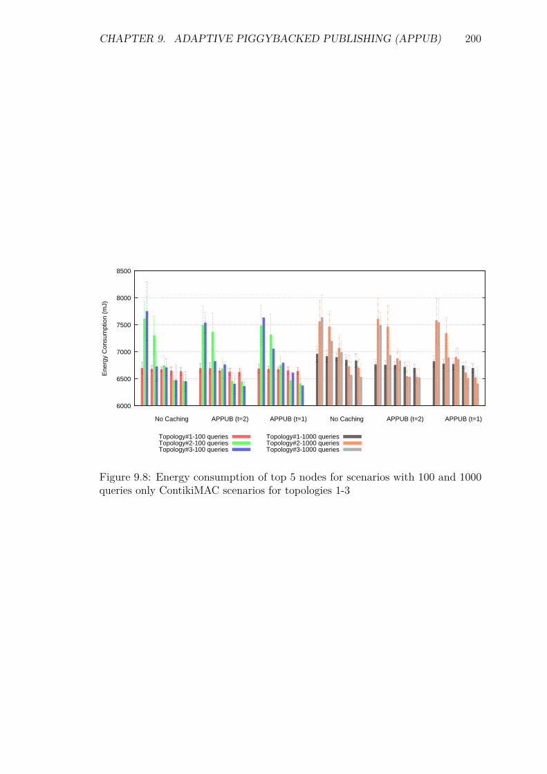
CHAPTER 9. ADAPTIVE PIGGYBACKED PUBLISHING (APPUB) 200
6000
6500
7000
7500
8000
8500
Ene
rgy
Con
sum
ptio
n (m
J)
Topology#1-100 queriesTopology#2-100 queriesTopology#3-100 queries
Topology#1-1000 queriesTopology#2-1000 queriesTopology#3-1000 queries
APPUB (t=1)APPUB (t=2)No CachingAPPUB (t=1)APPUB (t=2)No Caching
Figure 9.8: Energy consumption of top 5 nodes for scenarios with 100 and 1000queries only ContikiMAC scenarios for topologies 1-3
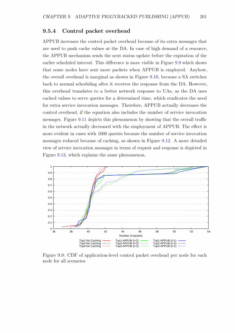
CHAPTER 9. ADAPTIVE PIGGYBACKED PUBLISHING (APPUB) 201
9.5.4 Control packet overhead
APPUB increases the control packet overhead because of its extra messages thatare used to push cache values at the DA. In case of high demand of a resource,the APPUB mechanism sends the next status update before the expiration of theearlier scheduled interval. This difference is more visible in Figure 9.9 which showsthat some nodes have sent more packets when APPUB is employed. Anyhow,the overall overhead is marginal as shown in Figure 9.10, because a SA switchesback to normal scheduling after it receives the response from the DA. However,this overhead translates to a better network response to UAs, as the DA usescached values to serve queries for a determined time, which eradicates the needfor extra service invocation messages. Therefore, APPUB actually decreases thecontrol overhead, if the equation also includes the number of service invocationmessages. Figure 9.11 depicts this phenomenon by showing that the overall trafficin the network actually decreased with the employment of APPUB. The effect ismore evident in cases with 1000 queries because the number of service invocationmessages reduced because of caching, as shown in Figure 9.12. A more detailedview of service invocation messages in terms of request and response is depicted inFigure 9.13, which explains the same phenomenon.
0
0.1
0.2
0.3
0.4
0.5
0.6
0.7
0.8
0.9
1
36 38 40 42 44 46 48 50 52 54
Number of packets
Top1-No CachingTop2-No CachingTop3-No Caching
Top1-APPUB (t=2)Top2-APPUB (t=2)Top3-APPUB (t=2)
Top1-APPUB (t=1)Top2-APPUB (t=1)Top3-APPUB (t=1)
Figure 9.9: CDF of application-level control packet overhead per node for eachnode for all scenarios
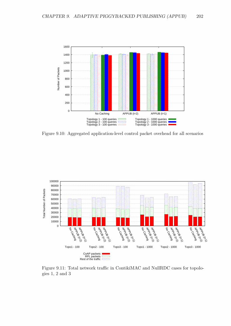
CHAPTER 9. ADAPTIVE PIGGYBACKED PUBLISHING (APPUB) 202
0
200
400
600
800
1000
1200
1400
1600
No Caching APPUB (t=2) APPUB (t=1)
Num
ber
of P
acke
ts
Topology 1 - 100 queriesTopology 2 - 100 queriesTopology 3 - 100 queries
Topology 1 - 1000 queriesTopology 2 - 1000 queriesTopology 3 - 1000 queries
Figure 9.10: Aggregated application-level control packet overhead for all scenarios
0
10000
20000
30000
40000
50000
60000
70000
80000
90000
100000
No C
achingA
PP
UB
(t=2)A
PP
UB
(t=1)
No C
achingA
PP
UB
(t=2)A
PP
UB
(t=1)
No C
achingA
PP
UB
(t=2)A
PP
UB
(t=1)
No C
achingA
PP
UB
(t=2)A
PP
UB
(t=1)
No C
achingA
PP
UB
(t=2)A
PP
UB
(t=1)
No C
achingA
PP
UB
(t=2)A
PP
UB
(t=1)
Tot
al N
umbe
r of
Pac
kets
CoAP packetsRPL packets
Rest of the traffic
Topo3 - 1000Topo2 - 1000Topo1 - 1000Topo3 - 100Topo2 - 100Topo1 - 100
Figure 9.11: Total network traffic in ContikiMAC and NullRDC cases for topolo-gies 1, 2 and 3
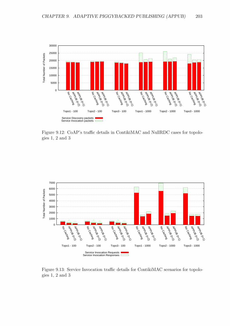
CHAPTER 9. ADAPTIVE PIGGYBACKED PUBLISHING (APPUB) 203
0
5000
10000
15000
20000
25000
30000
No C
achingA
PP
UB
(t=2)A
PP
UB
(t=1)
No C
achingA
PP
UB
(t=2)A
PP
UB
(t=1)
No C
achingA
PP
UB
(t=2)A
PP
UB
(t=1)
No C
achingA
PP
UB
(t=2)A
PP
UB
(t=1)
No C
achingA
PP
UB
(t=2)A
PP
UB
(t=1)
No C
achingA
PP
UB
(t=2)A
PP
UB
(t=1)
Tot
al N
umbe
r of
Pac
kets
Service Discovery packetsService Invocation packets
Topo3 - 1000Topo2 - 1000Topo1 - 1000Topo3 - 100Topo2 - 100Topo1 - 100
Figure 9.12: CoAP’s traffic details in ContikiMAC and NullRDC cases for topolo-gies 1, 2 and 3
0
1000
2000
3000
4000
5000
6000
7000
No C
achingA
PP
UB
(t=2)A
PP
UB
(t=1)
No C
achingA
PP
UB
(t=2)A
PP
UB
(t=1)
No C
achingA
PP
UB
(t=2)A
PP
UB
(t=1)
No C
achingA
PP
UB
(t=2)A
PP
UB
(t=1)
No C
achingA
PP
UB
(t=2)A
PP
UB
(t=1)
No C
achingA
PP
UB
(t=2)A
PP
UB
(t=1)
Tot
al N
umbe
r of
Pac
kets
Service Invocation RequestsService Invocation Responses
Topo3 - 1000Topo2 - 1000Topo1 - 1000Topo3 - 100Topo2 - 100Topo1 - 100
Figure 9.13: Service Invocation traffic details for ContikiMAC scenarios for topolo-gies 1, 2 and 3
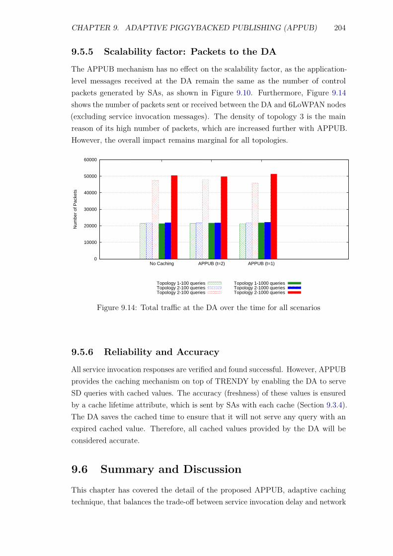
CHAPTER 9. ADAPTIVE PIGGYBACKED PUBLISHING (APPUB) 204
9.5.5 Scalability factor: Packets to the DA
The APPUB mechanism has no effect on the scalability factor, as the application-level messages received at the DA remain the same as the number of controlpackets generated by SAs, as shown in Figure 9.10. Furthermore, Figure 9.14shows the number of packets sent or received between the DA and 6LoWPAN nodes(excluding service invocation messages). The density of topology 3 is the mainreason of its high number of packets, which are increased further with APPUB.However, the overall impact remains marginal for all topologies.
0
10000
20000
30000
40000
50000
60000
No Caching APPUB (t=2) APPUB (t=1)
Num
ber
of P
acke
ts
Topology 1-100 queriesTopology 2-100 queriesTopology 2-100 queries
Topology 1-1000 queriesTopology 2-1000 queriesTopology 2-1000 queries
Figure 9.14: Total traffic at the DA over the time for all scenarios
9.5.6 Reliability and Accuracy
All service invocation responses are verified and found successful. However, APPUBprovides the caching mechanism on top of TRENDY by enabling the DA to serveSD queries with cached values. The accuracy (freshness) of these values is ensuredby a cache lifetime attribute, which is sent by SAs with each cache (Section 9.3.4).The DA saves the cached time to ensure that it will not serve any query with anexpired cached value. Therefore, all cached values provided by the DA will beconsidered accurate.
9.6 Summary and Discussion
This chapter has covered the detail of the proposed APPUB, adaptive cachingtechnique, that balances the trade-off between service invocation delay and network
CHAPTER 9. ADAPTIVE PIGGYBACKED PUBLISHING (APPUB) 205
efficiency. This method provides an alternative to proxy behaviour by reactingto the increasing number of service invocations. It adapts to the demand of aresource for caching rather than blindly caching all resources in a network. EachSA implements APPUB functionality to reduce the burden of service invocationsby sending cached values and corresponding lifetime values to the registry. Thismechanism offers multiple benefits: it decreases the service invocation delay andalso allows service hosts to share their load with the resource directory.
Several simulation experiments with emulated hardware nodes validate thebenefit of using APPUB technique in terms of low service invocation delay, overallcontrol packet overhead and energy consumption. The evaluation of the resultssupports the efficiency of APPUB, but it also draws some important conclusions.The density of a network plays a significant role in increasing the overall packetoverhead of the network, which is further augmented by the extra packets used forcaching. Nevertheless, the employment of APPUB reduces the number of serviceinvocation messages and consequently, decreases the overhead of a constrainednetwork. In addition, the low service invocation delay with APPUB improves theuser experience. However, this benefit comes only when the network is enoughbusy and maintained cache is being used by the DA to serve the queries, so itdepends on the carefully chosen sensitivity-level of the APPUB hit-count threshold.This research project arguments that it should be left to the ease of a SA, whichcan choose a hit count threshold depending on its available resources. In this case,different SAs are allowed to have a diverse range of threshold values. Even though,this makes APPUB a PUSH-based approach, it still can face challenging situationswhere high-capacity nodes can have high threshold values and can cost moreenergy for constrained nodes within a multi-hop network. This can be improvedby changing the RPL OF settings, so the high-capacity nodes remain on high levelof a DODAG tree and never use a path of constrained nodes. Another perspectivewhich is out of scope of this thesis is the case of a dense network where a DODAG’sroot has many nodes at the first level that increases neighbour discovery trafficand consequently, incurs high delays. Furthermore, a node can select a lifetime forits cache value depending on its constraints and the criteria and requirements of anetwork. It can use any algorithm to change this lifetime value adaptively.
The next chapter explains the effect of combining different TRENDY techniquesproposed in Chapters 7, 8 and 9.
Chapter 10
TRENDY: a Trend-based ServiceDiscovery Solution for the IoT
10.1 Introduction
Chapters 7, 8 and 9 have introduced new adaptive and grouping techniques forthe TRENDY protocol to cope with the IoT requirements gathered in Chapter 4.The proposed techniques require small changes in TRENDY’s message formats(Section 5.11). Furthermore, new rules are needed when a combination of thesetechniques is used together. This chapter explains the usage of TRENDY with thecombination of proposed techniques. In addition, it discusses the evaluation doneby undertaking experiments to analyse the effect of using a combination of thesetechniques in a network.
10.2 TRENDY Protocol with AdaptiveTechniques
This section describes the TRENDY protocol with the integration of adaptivetimer, APPUB and grouping techniques.
10.2.1 Message Format
The merger of timer, grouping and APPUB together with TRENDY requiresonly one small update in the response of the DA for status maintenance updates(Section 5.11.2). In the new format, the DA sends both trendy_counter andproxy_mode in the payload to the SA. Figure 10.1 shows the order of attributesin the updated message format. Grouping mechanism requires no change in theTRENDY message formats (Section 5.11); however, the YGL message now needs to
206
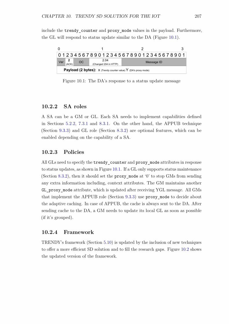
CHAPTER 10. TRENDY SD SOLUTION FOR THE IOT 207
include the trendy_counter and proxy_mode values in the payload. Furthermore,the GL will respond to status update similar to the DA (Figure 10.1).
� � � � � � � � � � � � � � � � � � � � � � � � � ��� ��
������� �� ��� � � �� ���� ������ ������� �� !" # ��� $����
� � � �
�� �&�
�'����)��*�� ��� +� ,��-�
.�""�*� /�
Figure 10.1: The DA’s response to a status update message
10.2.2 SA roles
A SA can be a GM or GL. Each SA needs to implement capabilities definedin Sections 5.2.2, 7.3.1 and 8.3.1. On the other hand, the APPUB technique(Section 9.3.3) and GL role (Section 8.3.2) are optional features, which can beenabled depending on the capability of a SA.
10.2.3 Policies
All GLs need to specify the trendy_counter and proxy_mode attributes in responseto status updates, as shown in Figure 10.1. If a GL only supports status maintenance(Section 8.3.2), then it should set the proxy_mode at ‘0’ to stop GMs from sendingany extra information including, context attributes. The GM maintains anotherGL_proxy_mode attribute, which is updated after receiving YGL message. All GMsthat implement the APPUB role (Section 9.3.3) use proxy_mode to decide aboutthe adaptive caching. In case of APPUB, the cache is always sent to the DA. Aftersending cache to the DA, a GM needs to update its local GL as soon as possible(if it’s grouped).
10.2.4 Framework
TRENDY’s framework (Section 5.10) is updated by the inclusion of new techniquesto offer a more efficient SD solution and to fill the research gaps. Figure 10.2 showsthe updated version of the framework.
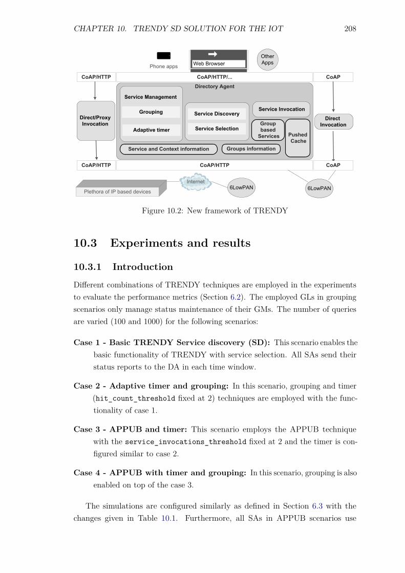
CHAPTER 10. TRENDY SD SOLUTION FOR THE IOT 208
��������� ���
��� ���������� ��
��������������
������ �� � � �� ������
��������
�������
�������
������� �����
������� ����������
������� ���������
������� ���������
������� ���������
������� ��� ������ �����������
��� �� �� �
����������������������
��
���������������������
!������������
������ �����������
������
��������"""
������� �� �������
Figure 10.2: New framework of TRENDY
10.3 Experiments and results
10.3.1 Introduction
Different combinations of TRENDY techniques are employed in the experimentsto evaluate the performance metrics (Section 6.2). The employed GLs in groupingscenarios only manage status maintenance of their GMs. The number of queriesare varied (100 and 1000) for the following scenarios:
Case 1 - Basic TRENDY Service discovery (SD): This scenario enables thebasic functionality of TRENDY with service selection. All SAs send theirstatus reports to the DA in each time window.
Case 2 - Adaptive timer and grouping: In this scenario, grouping and timer(hit_count_threshold fixed at 2) techniques are employed with the func-tionality of case 1.
Case 3 - APPUB and timer: This scenario employs the APPUB techniquewith the service_invocations_threshold fixed at 2 and the timer is con-figured similar to case 2.
Case 4 - APPUB with timer and grouping: In this scenario, grouping is alsoenabled on top of the case 3.
The simulations are configured similarly as defined in Section 6.3 with thechanges given in Table 10.1. Furthermore, all SAs in APPUB scenarios use
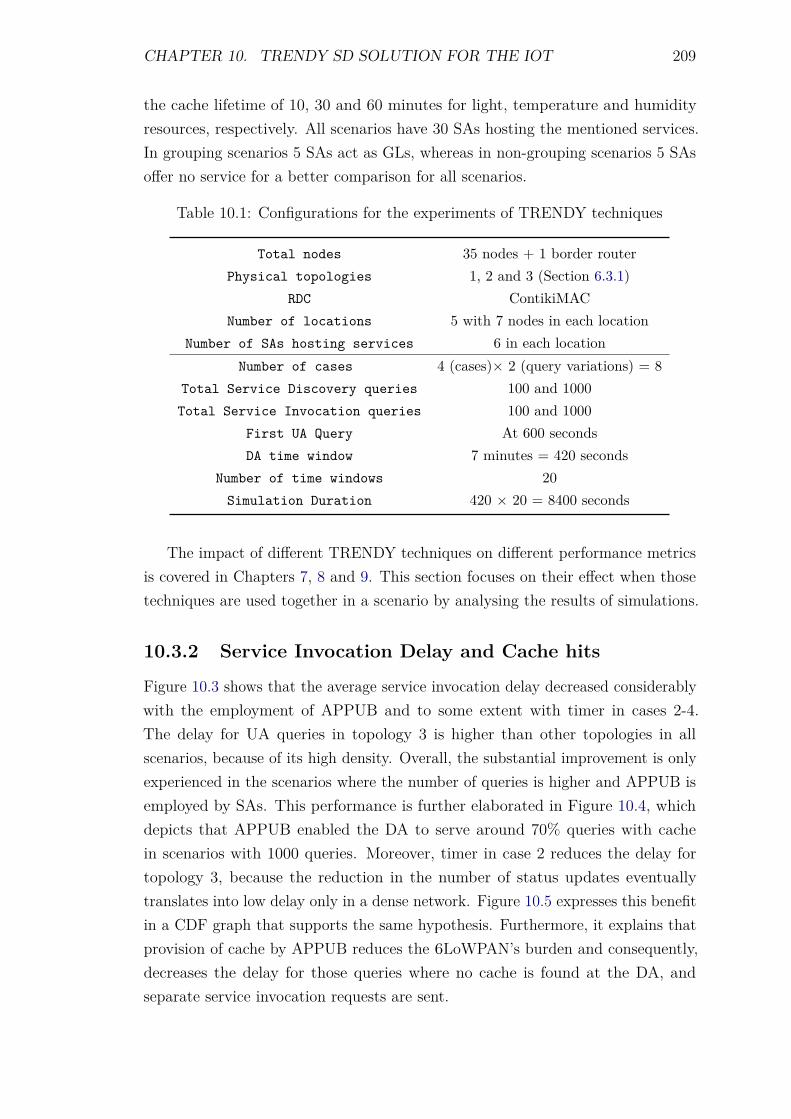
CHAPTER 10. TRENDY SD SOLUTION FOR THE IOT 209
the cache lifetime of 10, 30 and 60 minutes for light, temperature and humidityresources, respectively. All scenarios have 30 SAs hosting the mentioned services.In grouping scenarios 5 SAs act as GLs, whereas in non-grouping scenarios 5 SAsoffer no service for a better comparison for all scenarios.
Table 10.1: Configurations for the experiments of TRENDY techniques
Total nodes 35 nodes + 1 border routerPhysical topologies 1, 2 and 3 (Section 6.3.1)
RDC ContikiMACNumber of locations 5 with 7 nodes in each location
Number of SAs hosting services 6 in each locationNumber of cases 4 (cases)× 2 (query variations) = 8
Total Service Discovery queries 100 and 1000Total Service Invocation queries 100 and 1000
First UA Query At 600 secondsDA time window 7 minutes = 420 seconds
Number of time windows 20Simulation Duration 420 × 20 = 8400 seconds
The impact of different TRENDY techniques on different performance metricsis covered in Chapters 7, 8 and 9. This section focuses on their effect when thosetechniques are used together in a scenario by analysing the results of simulations.
10.3.2 Service Invocation Delay and Cache hits
Figure 10.3 shows that the average service invocation delay decreased considerablywith the employment of APPUB and to some extent with timer in cases 2-4.The delay for UA queries in topology 3 is higher than other topologies in allscenarios, because of its high density. Overall, the substantial improvement is onlyexperienced in the scenarios where the number of queries is higher and APPUB isemployed by SAs. This performance is further elaborated in Figure 10.4, whichdepicts that APPUB enabled the DA to serve around 70% queries with cachein scenarios with 1000 queries. Moreover, timer in case 2 reduces the delay fortopology 3, because the reduction in the number of status updates eventuallytranslates into low delay only in a dense network. Figure 10.5 expresses this benefitin a CDF graph that supports the same hypothesis. Furthermore, it explains thatprovision of cache by APPUB reduces the 6LoWPAN’s burden and consequently,decreases the delay for those queries where no cache is found at the DA, andseparate service invocation requests are sent.
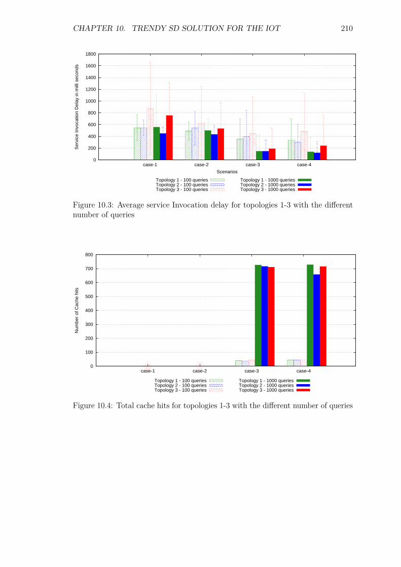
CHAPTER 10. TRENDY SD SOLUTION FOR THE IOT 210
0
200
400
600
800
1000
1200
1400
1600
1800
case-1 case-2 case-3 case-4
Ser
vice
Invo
catio
n D
elay
in m
illi s
econ
ds
Scenarios
Topology 1 - 100 queriesTopology 2 - 100 queriesTopology 3 - 100 queries
Topology 1 - 1000 queriesTopology 2 - 1000 queriesTopology 3 - 1000 queries
Figure 10.3: Average service Invocation delay for topologies 1-3 with the differentnumber of queries
0
100
200
300
400
500
600
700
800
case-1 case-2 case-3 case-4
Num
ber
of C
ache
hits
Topology 1 - 100 queriesTopology 2 - 100 queriesTopology 3 - 100 queries
Topology 1 - 1000 queriesTopology 2 - 1000 queriesTopology 3 - 1000 queries
Figure 10.4: Total cache hits for topologies 1-3 with the different number of queries
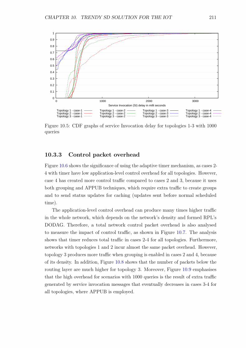
CHAPTER 10. TRENDY SD SOLUTION FOR THE IOT 211
0
0.1
0.2
0.3
0.4
0.5
0.6
0.7
0.8
0.9
1
0 1000 2000 3000
Service Invocation (SI) delay in milli seconds
Topology 1 - case-1Topology 2 - case-1Topology 3 - case-1
Topology 1 - case-2Topology 2 - case-2Topology 3 - case-2
Topology 1 - case-3Topology 2 - case-3Topology 3 - case-3
Topology 1 - case-4Topology 2 - case-4Topology 3 - case-4
Figure 10.5: CDF graphs of service Invocation delay for topologies 1-3 with 1000queries
10.3.3 Control packet overhead
Figure 10.6 shows the significance of using the adaptive timer mechanism, as cases 2-4 with timer have low application-level control overhead for all topologies. However,case 4 has created more control traffic compared to cases 2 and 3, because it usesboth grouping and APPUB techniques, which require extra traffic to create groupsand to send status updates for caching (updates sent before normal scheduledtime).
The application-level control overhead can produce many times higher trafficin the whole network, which depends on the network’s density and formed RPL’sDODAG. Therefore, a total network control packet overhead is also analysedto measure the impact of control traffic, as shown in Figure 10.7. The analysisshows that timer reduces total traffic in cases 2-4 for all topologies. Furthermore,networks with topologies 1 and 2 incur almost the same packet overhead. However,topology 3 produces more traffic when grouping is enabled in cases 2 and 4, becauseof its density. In addition, Figure 10.8 shows that the number of packets below therouting layer are much higher for topology 3. Moreover, Figure 10.9 emphasisesthat the high overhead for scenarios with 1000 queries is the result of extra trafficgenerated by service invocation messages that eventually decreases in cases 3-4 forall topologies, where APPUB is employed.
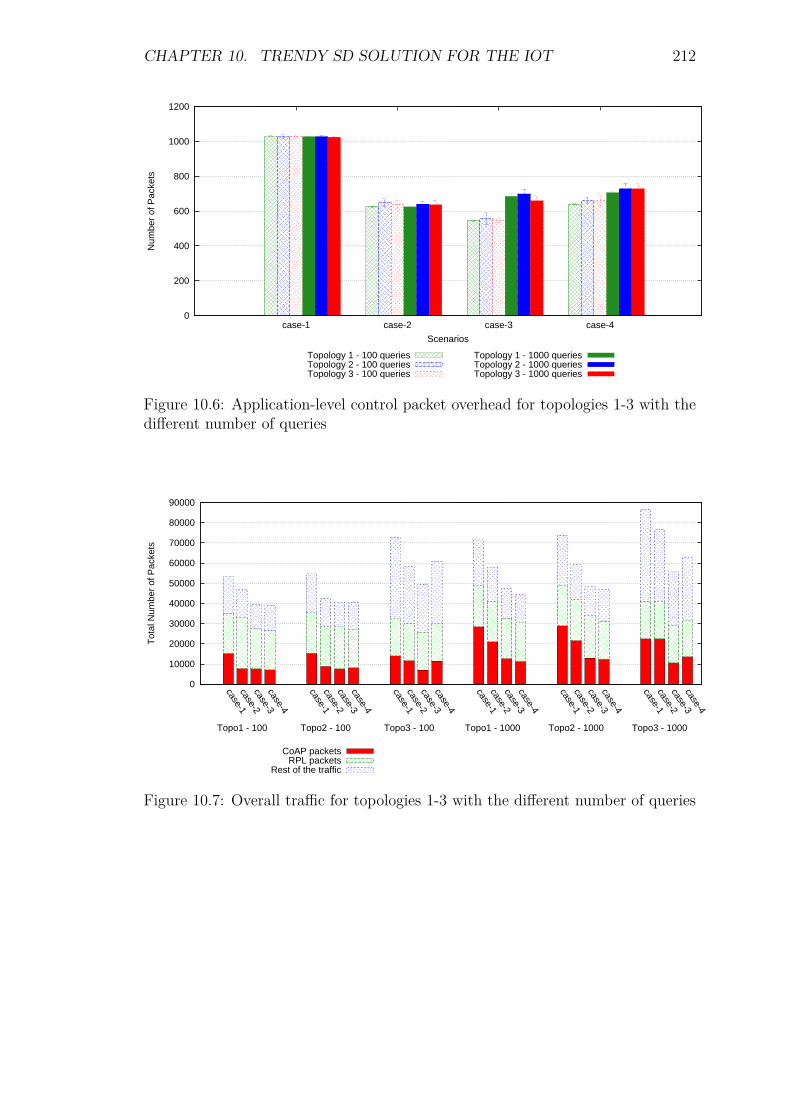
CHAPTER 10. TRENDY SD SOLUTION FOR THE IOT 212
0
200
400
600
800
1000
1200
case-1 case-2 case-3 case-4
Num
ber
of P
acke
ts
Scenarios
Topology 1 - 100 queriesTopology 2 - 100 queriesTopology 3 - 100 queries
Topology 1 - 1000 queriesTopology 2 - 1000 queriesTopology 3 - 1000 queries
Figure 10.6: Application-level control packet overhead for topologies 1-3 with thedifferent number of queries
0
10000
20000
30000
40000
50000
60000
70000
80000
90000
case-1case-2case-3case-4
case-1case-2case-3case-4
case-1case-2case-3case-4
case-1case-2case-3case-4
case-1case-2case-3case-4
case-1case-2case-3case-4
Tot
al N
umbe
r of
Pac
kets
CoAP packetsRPL packets
Rest of the traffic
Topo3 - 1000Topo2 - 1000Topo1 - 1000Topo3 - 100Topo2 - 100Topo1 - 100
Figure 10.7: Overall traffic for topologies 1-3 with the different number of queries
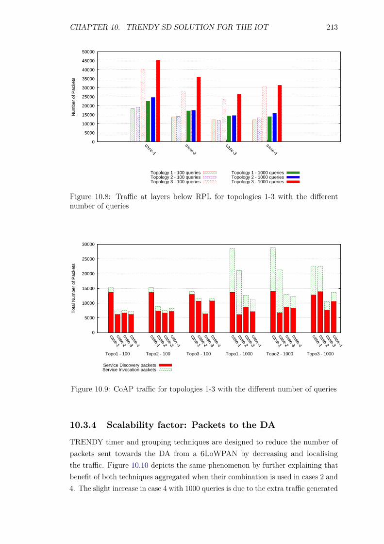
CHAPTER 10. TRENDY SD SOLUTION FOR THE IOT 213
0
5000
10000
15000
20000
25000
30000
35000
40000
45000
50000
case-1
case-2
case-3
case-4
Num
ber
of P
acke
ts
Topology 1 - 100 queriesTopology 2 - 100 queriesTopology 3 - 100 queries
Topology 1 - 1000 queriesTopology 2 - 1000 queriesTopology 3 - 1000 queries
Figure 10.8: Traffic at layers below RPL for topologies 1-3 with the differentnumber of queries
0
5000
10000
15000
20000
25000
30000
case-1case-2case-3case-4
case-1case-2case-3case-4
case-1case-2case-3case-4
case-1case-2case-3case-4
case-1case-2case-3case-4
case-1case-2case-3case-4
Tot
al N
umbe
r of
Pac
kets
Service Discovery packetsService Invocation packets
Topo3 - 1000Topo2 - 1000Topo1 - 1000Topo3 - 100Topo2 - 100Topo1 - 100
Figure 10.9: CoAP traffic for topologies 1-3 with the different number of queries
10.3.4 Scalability factor: Packets to the DA
TRENDY timer and grouping techniques are designed to reduce the number ofpackets sent towards the DA from a 6LoWPAN by decreasing and localisingthe traffic. Figure 10.10 depicts the same phenomenon by further explaining thatbenefit of both techniques aggregated when their combination is used in cases 2 and4. The slight increase in case 4 with 1000 queries is due to the extra traffic generated
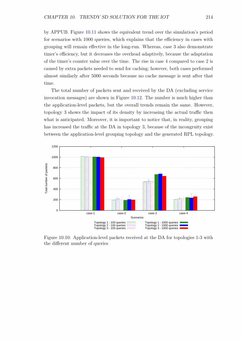
CHAPTER 10. TRENDY SD SOLUTION FOR THE IOT 214
by APPUB. Figure 10.11 shows the equivalent trend over the simulation’s periodfor scenarios with 1000 queries, which explains that the efficiency in cases withgrouping will remain effective in the long-run. Whereas, case 3 also demonstratetimer’s efficiency, but it decreases the overhead adaptively, because the adaptationof the timer’s counter value over the time. The rise in case 4 compared to case 2 iscaused by extra packets needed to send for caching; however, both cases performedalmost similarly after 5000 seconds because no cache message is sent after thattime.
The total number of packets sent and received by the DA (excluding serviceinvocation messages) are shown in Figure 10.12. The number is much higher thanthe application-level packets, but the overall trends remain the same. However,topology 3 shows the impact of its density by increasing the actual traffic thenwhat is anticipated. Moreover, it is important to notice that, in reality, groupinghas increased the traffic at the DA in topology 3, because of the incongruity existbetween the application-level grouping topology and the generated RPL topology.
0
200
400
600
800
1000
1200
case-1 case-2 case-3 case-4
Tot
al n
umbe
r of
pac
kets
Scenarios
Topology 1 - 100 queriesTopology 2 - 100 queriesTopology 3 - 100 queries
Topology 1 - 1000 queriesTopology 2 - 1000 queriesTopology 3 - 1000 queries
Figure 10.10: Application-level packets received at the DA for topologies 1-3 withthe different number of queries
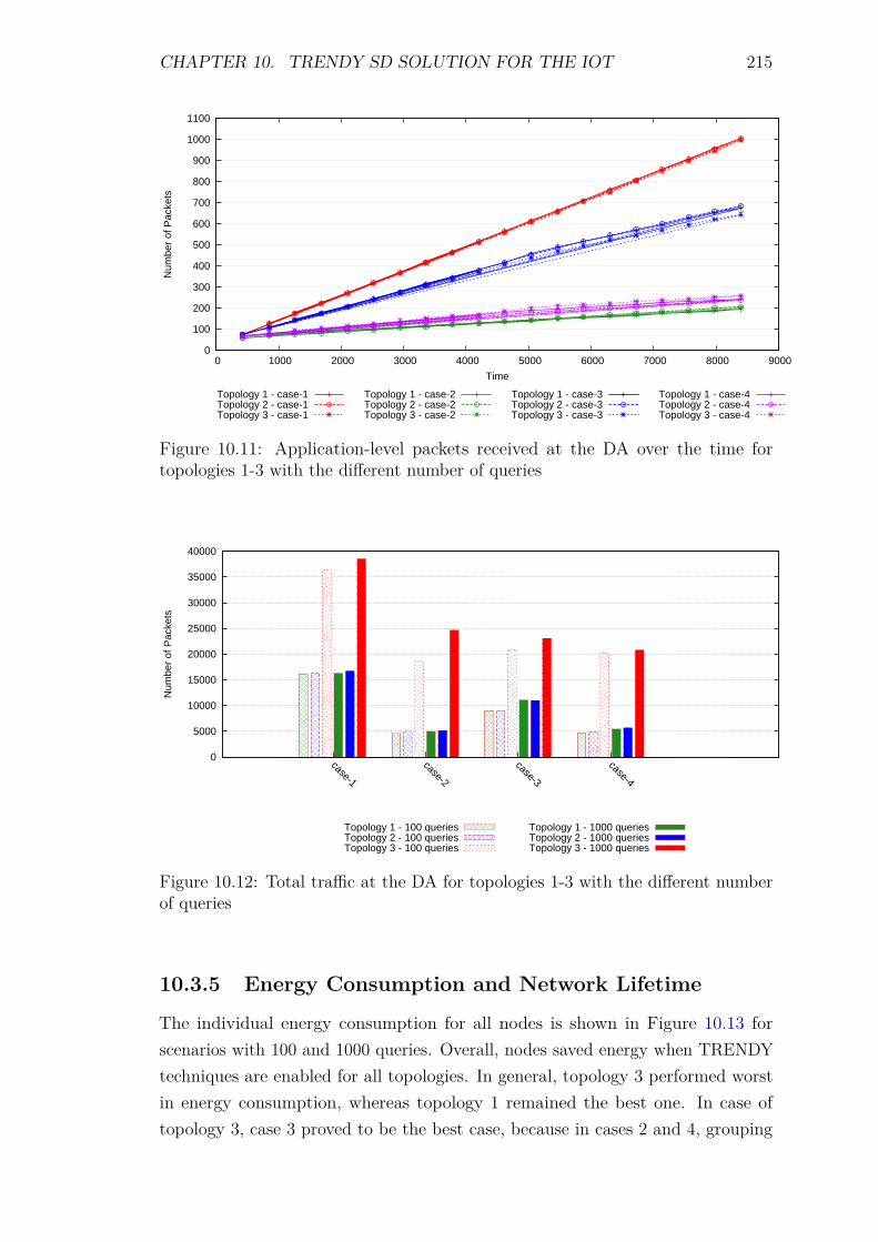
CHAPTER 10. TRENDY SD SOLUTION FOR THE IOT 215
0
100
200
300
400
500
600
700
800
900
1000
1100
0 1000 2000 3000 4000 5000 6000 7000 8000 9000
Num
ber
of P
acke
ts
Time
Topology 1 - case-1Topology 2 - case-1Topology 3 - case-1
Topology 1 - case-2Topology 2 - case-2Topology 3 - case-2
Topology 1 - case-3Topology 2 - case-3Topology 3 - case-3
Topology 1 - case-4Topology 2 - case-4Topology 3 - case-4
Figure 10.11: Application-level packets received at the DA over the time fortopologies 1-3 with the different number of queries
0
5000
10000
15000
20000
25000
30000
35000
40000
case-1
case-2
case-3
case-4
Num
ber
of P
acke
ts
Topology 1 - 100 queriesTopology 2 - 100 queriesTopology 3 - 100 queries
Topology 1 - 1000 queriesTopology 2 - 1000 queriesTopology 3 - 1000 queries
Figure 10.12: Total traffic at the DA for topologies 1-3 with the different numberof queries
10.3.5 Energy Consumption and Network Lifetime
The individual energy consumption for all nodes is shown in Figure 10.13 forscenarios with 100 and 1000 queries. Overall, nodes saved energy when TRENDYtechniques are enabled for all topologies. In general, topology 3 performed worstin energy consumption, whereas topology 1 remained the best one. In case oftopology 3, case 3 proved to be the best case, because in cases 2 and 4, grouping
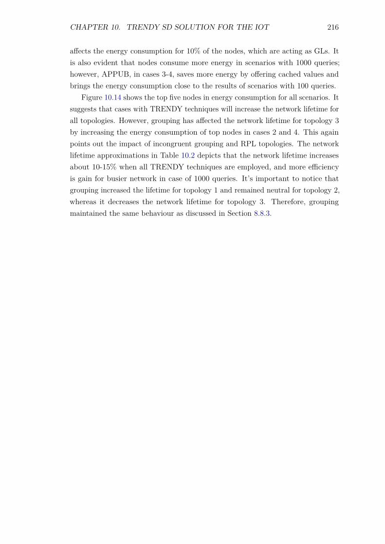
CHAPTER 10. TRENDY SD SOLUTION FOR THE IOT 216
affects the energy consumption for 10% of the nodes, which are acting as GLs. Itis also evident that nodes consume more energy in scenarios with 1000 queries;however, APPUB, in cases 3-4, saves more energy by offering cached values andbrings the energy consumption close to the results of scenarios with 100 queries.
Figure 10.14 shows the top five nodes in energy consumption for all scenarios. Itsuggests that cases with TRENDY techniques will increase the network lifetime forall topologies. However, grouping has affected the network lifetime for topology 3by increasing the energy consumption of top nodes in cases 2 and 4. This againpoints out the impact of incongruent grouping and RPL topologies. The networklifetime approximations in Table 10.2 depicts that the network lifetime increasesabout 10-15% when all TRENDY techniques are employed, and more efficiencyis gain for busier network in case of 1000 queries. It’s important to notice thatgrouping increased the lifetime for topology 1 and remained neutral for topology 2,whereas it decreases the network lifetime for topology 3. Therefore, groupingmaintained the same behaviour as discussed in Section 8.8.3.
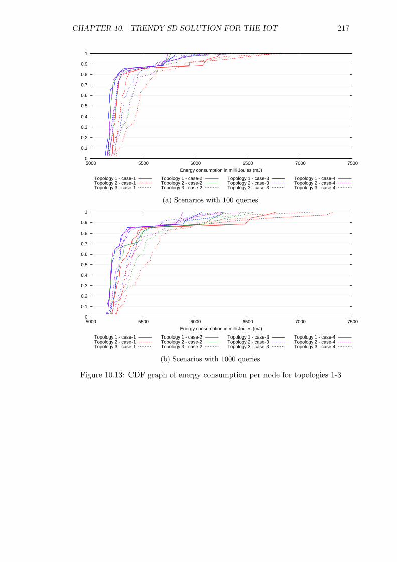
CHAPTER 10. TRENDY SD SOLUTION FOR THE IOT 217
0
0.1
0.2
0.3
0.4
0.5
0.6
0.7
0.8
0.9
1
5000 5500 6000 6500 7000 7500
Energy consumption in milli Joules (mJ)
Topology 1 - case-1Topology 2 - case-1Topology 3 - case-1
Topology 1 - case-2Topology 2 - case-2Topology 3 - case-2
Topology 1 - case-3Topology 2 - case-3Topology 3 - case-3
Topology 1 - case-4Topology 2 - case-4Topology 3 - case-4
(a) Scenarios with 100 queries
0
0.1
0.2
0.3
0.4
0.5
0.6
0.7
0.8
0.9
1
5000 5500 6000 6500 7000 7500
Energy consumption in milli Joules (mJ)
Topology 1 - case-1Topology 2 - case-1Topology 3 - case-1
Topology 1 - case-2Topology 2 - case-2Topology 3 - case-2
Topology 1 - case-3Topology 2 - case-3Topology 3 - case-3
Topology 1 - case-4Topology 2 - case-4Topology 3 - case-4
(b) Scenarios with 1000 queries
Figure 10.13: CDF graph of energy consumption per node for topologies 1-3
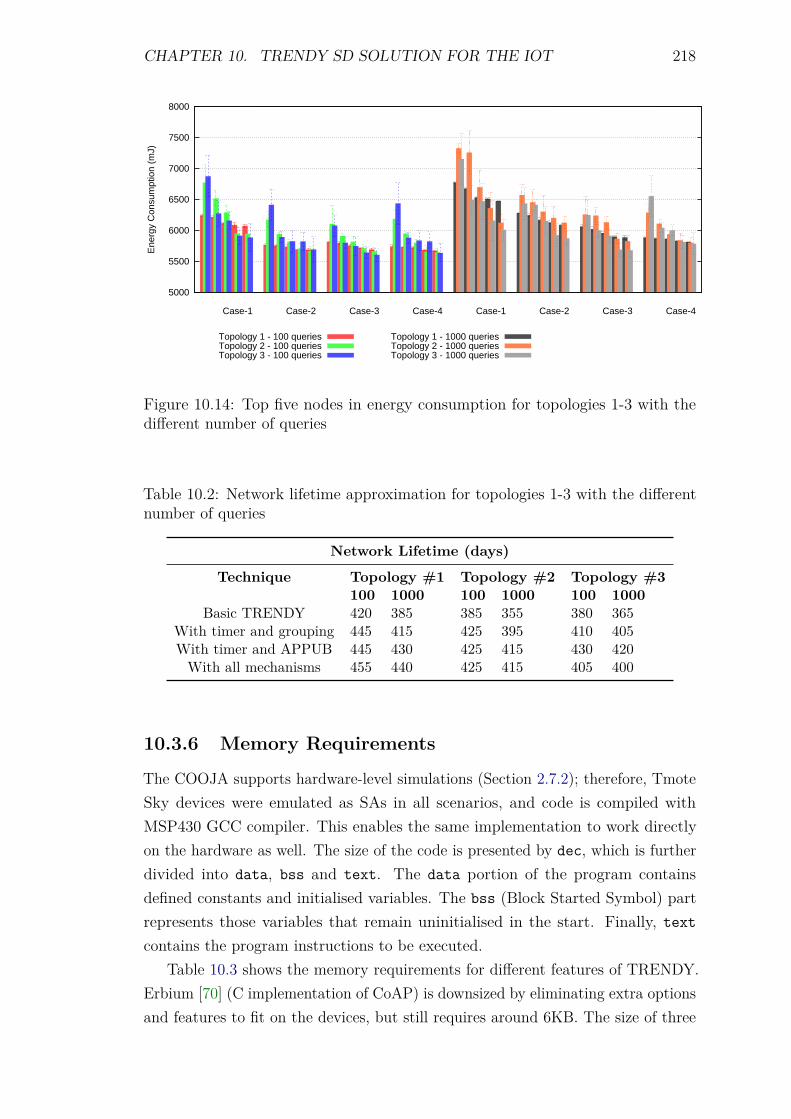
CHAPTER 10. TRENDY SD SOLUTION FOR THE IOT 218
5000
5500
6000
6500
7000
7500
8000
Ene
rgy
Con
sum
ptio
n (m
J)
Topology 1 - 100 queriesTopology 2 - 100 queriesTopology 3 - 100 queries
Topology 1 - 1000 queriesTopology 2 - 1000 queriesTopology 3 - 1000 queries
Case-4Case-3Case-2Case-1Case-4Case-3Case-2Case-1
Figure 10.14: Top five nodes in energy consumption for topologies 1-3 with thedifferent number of queries
Table 10.2: Network lifetime approximation for topologies 1-3 with the differentnumber of queries
Network Lifetime (days)
Technique Topology #1 Topology #2 Topology #3100 1000 100 1000 100 1000
Basic TRENDY 420 385 385 355 380 365With timer and grouping 445 415 425 395 410 405With timer and APPUB 445 430 425 415 430 420With all mechanisms 455 440 425 415 405 400
10.3.6 Memory Requirements
The COOJA supports hardware-level simulations (Section 2.7.2); therefore, TmoteSky devices were emulated as SAs in all scenarios, and code is compiled withMSP430 GCC compiler. This enables the same implementation to work directlyon the hardware as well. The size of the code is presented by dec, which is furtherdivided into data, bss and text. The data portion of the program containsdefined constants and initialised variables. The bss (Block Started Symbol) partrepresents those variables that remain uninitialised in the start. Finally, textcontains the program instructions to be executed.
Table 10.3 shows the memory requirements for different features of TRENDY.Erbium [70] (C implementation of CoAP) is downsized by eliminating extra optionsand features to fit on the devices, but still requires around 6KB. The size of three
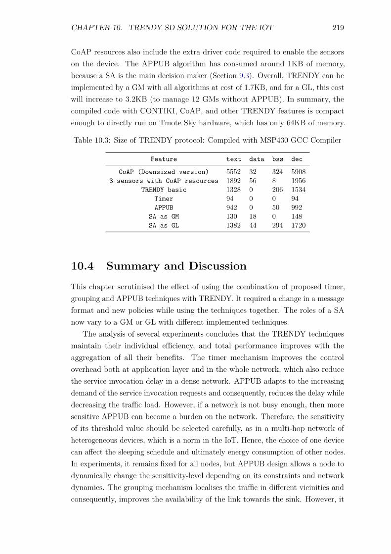
CHAPTER 10. TRENDY SD SOLUTION FOR THE IOT 219
CoAP resources also include the extra driver code required to enable the sensorson the device. The APPUB algorithm has consumed around 1KB of memory,because a SA is the main decision maker (Section 9.3). Overall, TRENDY can beimplemented by a GM with all algorithms at cost of 1.7KB, and for a GL, this costwill increase to 3.2KB (to manage 12 GMs without APPUB). In summary, thecompiled code with CONTIKI, CoAP, and other TRENDY features is compactenough to directly run on Tmote Sky hardware, which has only 64KB of memory.
Table 10.3: Size of TRENDY protocol: Compiled with MSP430 GCC Compiler
Feature text data bss dec
CoAP (Downsized version) 5552 32 324 59083 sensors with CoAP resources 1892 56 8 1956
TRENDY basic 1328 0 206 1534Timer 94 0 0 94APPUB 942 0 50 992
SA as GM 130 18 0 148SA as GL 1382 44 294 1720
10.4 Summary and Discussion
This chapter scrutinised the effect of using the combination of proposed timer,grouping and APPUB techniques with TRENDY. It required a change in a messageformat and new policies while using the techniques together. The roles of a SAnow vary to a GM or GL with different implemented techniques.
The analysis of several experiments concludes that the TRENDY techniquesmaintain their individual efficiency, and total performance improves with theaggregation of all their benefits. The timer mechanism improves the controloverhead both at application layer and in the whole network, which also reducethe service invocation delay in a dense network. APPUB adapts to the increasingdemand of the service invocation requests and consequently, reduces the delay whiledecreasing the traffic load. However, if a network is not busy enough, then moresensitive APPUB can become a burden on the network. Therefore, the sensitivityof its threshold value should be selected carefully, as in a multi-hop network ofheterogeneous devices, which is a norm in the IoT. Hence, the choice of one devicecan affect the sleeping schedule and ultimately energy consumption of other nodes.In experiments, it remains fixed for all nodes, but APPUB design allows a node todynamically change the sensitivity-level depending on its constraints and networkdynamics. The grouping mechanism localises the traffic in different vicinities andconsequently, improves the availability of the link towards the sink. However, it

CHAPTER 10. TRENDY SD SOLUTION FOR THE IOT 220
is concluded from the analysis of the results that it actually makes the situationworse for GLs, if grouping topology is incongruent to RPL topology. Anyway, thiscan’t be an issue in those scenarios where a GL has better battery source andis a resource-rich device. Even though, the results of multiple topologies conveythat if RPL’s parameters are configured administratively to create more congruentDODAG, then situation becomes suitable for grouping to improve the performanceof a network.
The next chapter compares the TRENDY SD solution with other prospectivetechniques from different perspectives.
Chapter 11
Comparison with other solutions
11.1 Introduction
There is a plethora of SDPs devised for Ad-Hoc, MANET, WSN and IP networks(Chapter 3). Industry-standard IP-based SDPs including SLP, UPnP, JINI andSalutation are not directly applicable to 6LoWPANs because of their verbose andcomplex data formats, high communication overhead and dependence on protocols,which are unsuitable for constrained networks. On the other hand, the solutionsdesigned for constrained networks just focus on increasing the efficiency for asingle application (Section 3.9). Therefore, most of these existing standards donot address the issues which need a solution to balance the trade-off betweenthe requirements of the IoT and efficiency for constrained domains (Chapter 4).Consequently, this research project proposes TRENDY to provide context-awareSD and selection. Moreover, it devises the timer, grouping and APPUB techniquesfor adaptability to network dynamics to cope with the challenges.
This chapter covers the functionality based comparison of the proposed solu-tion with other suitable options for 6LoWPANs. Two protocols are selected forcomparison, which are the adaptations of existing widely used IP-based standards:uBonjour [64] (Bonjour Adaptation) and SSLP-based [18] (SLP Adaptation) SDsolutions. These adaptations have considered constraints of 6LoWPANs and havereduced the complexity, size and overhead of existing protocols. Furthermore, thosesolutions are backward compatible to their complex versions, but need a gatewayfor such a translation. Another option could be the IETF Resource directorywhich is closely related to TRENDY. However, it is still in a design phase, and canbenefit from the proposed techniques to enhance its performance. The proposedsolution focused on addressing the key requirements of efficiency, adaptability andcontext-awareness. This chapter qualitatively compares the proposed solution withthe selected protocols from different perspectives related to SD and its requirements
221
CHAPTER 11. COMPARISON WITH OTHER SOLUTIONS 222
in IoT environment.
11.2 Context-awareness
Context-awareness is an important feature that enables a user application to definea better SD query to search the relevant services in the IoT. Furthermore, it canenable a SD solution to assist the user application to select a better service basedon available context information.
uBonjour: uBonjour has no support for context-awareness. Thus, it only allowsthe query with a fixed DNS based URL.
SSLP-based solution: This solution is extended [19] to enable context-awareness,but no detail of context registration has been described. However, the ideaallows the user agents to send context-aware SD queries. Its service selectiononly considers proximity (close in hops) as a service selection criteria.
TRENDY: This SDP has focused on context-awareness by defining a defaultsimple attribute-value pair format to describe context attributes (Section 5.5);however, it allows the employment of any other semantic format as well.TRENDY allows a discovery query to define service types, location andother relevant information (e.g., semantic information). Its service selectionmechanism (Section 5.8) uses maintained context information including,battery source, distance (number of hops), remaining power and popularityto enable the discovery of an appropriate service based on user and network’scontext.
11.3 Extensibility
The IoT environment demands extensible solution to accommodate a range ofheterogeneous devices (resource-awareness) and new semantic formats for servicedescriptions. Following is the comparison of SD solutions from the extensibilityperspective:
uBonjour: uBonjour uses fixed service description format by only allowing DNSURI to describe a service. It has not described any specific roles for hetero-geneous devices.
SSLP-based solution: SSLP-based solution uses fixed SLP service types asservice descriptions. However, it describes two profiles for nodes: SA and
CHAPTER 11. COMPARISON WITH OTHER SOLUTIONS 223
master node. The master nodes serves as local registries and localises theinformation by enabling a hierarchical architecture.
TRENDY: TRENDY has a simple service description format, but allows theusage of any other format (Section 5.4). It proposes different roles withmodular design to enable nodes to implement distinctive features dependingon their capabilities (Section 10.2.2).
11.4 Interoperability
Interoperability of protocols and systems is important to allow their usage withother existing solutions.
uBonjour: uBonjour uses DNS-SD to offer interoperability with DNS infrastruc-ture, but it has not defined an efficient way to maintain a central directorywhile employing mDNS inside the network.
SSLP-based solution: SSLP-based solution offers interoperability with SLP;however, it requires an application gateway for translation between protocol.
TRENDY: TRENDY employs CoAP that enables the RESTful web serviceparadigm to offer an open and interoperable framework (Section 10.2.4). Itallows the discovery using either CoAP or HTTP, and central registry canbe updated to offer interoperability by passing services in many formats,including, WSDL and DNS-URIs (Section 5.11.3).
11.5 Constraints Considerations
Following is the list of the constraints discussed for each of the protocols beingcompared:
Devices with sleep cycles: uBonjour uses mDNS and multiple packets for ser-vice registration and status updates, which needs more data to be passed onin a multi-hop network and thus is an unsuitable choice for devices with sleepcycles. SSLP-based solution utilises unicast for discovery, but still requiresservice information to be communicated between different local directoriesand the DA. This demands high-bandwidth usage, as service status main-tenance is required at multiple places. TRENDY addresses this challenge inmultiple ways: it uses unicast and timer mechanism to decrease the controloverhead, and its APPUB technique allows the nodes to sleep more even incase of high number of service invocations.
CHAPTER 11. COMPARISON WITH OTHER SOLUTIONS 224
Code and Packet Size: All protocols have considered 6LoWPANs code andpacket size issues (Section 4.4.4), and can run on constrained devices withcompact packet size.
11.6 Dependencies
Following is the dependency list of all protocols being compared:
uBonjour: uBonjour requires multicast support.
SSLP-based solution: This needs an application gateway to translate betweenSLP and SSLP messages. In addition, local master nodes are required to bedeployed in each area.
TRENDY: This protocol requires CoAP-to-HTTP seamless proxy where a UAwants to use HTTP for service invocation (Section 10.2.4). Furthermore,some nodes are required to act as GLs to reap the benefits of the groupingmechanism.
11.7 Performance Metrics
The performance metrics for a SD solution consists of: Service Discovery delay,Service Invocation delay, energy consumption, scalability in terms of protocol’sarchitecture and control overhead (Section 6.2). This section compares TRENDYwith other solutions from these metrics perspectives.
11.7.1 Service Discovery delay
A UA mostly queries from outside the network in a IoT environment, which needsa centralised registry to deal with SD queries. Thus, in that case, all solutionswill perform similarly; however, the service discovery delay will be variable forqueries that are initiated from within a network as these solutions use differentarchitectures (Section 11.7.3).
11.7.2 Service Invocation support
A SD solution can support different levels of service invocation (Section 3.10.5).TRENDY provides service invocation support, and its APPUB technique providescached values to improve the service invocation delay. On the other hand, noneof the compared techniques support service invocation other than finding a hostdevice.
CHAPTER 11. COMPARISON WITH OTHER SOLUTIONS 225
11.7.3 Scalability
The scalability of a SD solution depends upon the architecture of a protocol andits behaviour in response to the increasing number of nodes and services within anetwork in terms of control overhead. The control overhead of a protocol is thesum of all service registration, advertisement and status update messages.
In a centralised architecture, all nodes register their services at the centralregistry, whereas in a distributed directory based architecture, all services areregistered to local registries. On the other hand, directory-less solutions allownodes to pro-actively advertise their services within vicinity, which are cached bytheir neighbours for a quick SD response to a user agent. This cached serviceinformation at a registry or neighbour node requires status maintenance to ensurethe reliability of SD responses, which is achieved by refreshing the status ofregistered services. However, this increases the control overhead of a protocol,and result in extra energy consumption of nodes and can also cause a bottleneckproblem in centralised architectures.
This section analyses the scalability in the context of control overhead of SDPsincluding, uBonjour, SSLP-based solution and TRENDY.
uBonjour: uBonjour uses a directory-less approach, which generates high multic-ast traffic to announce services in a vicinity that are cached by the neighbours.However, it still needs a centralised registry, e.g., service proxy [101] or amDNS daemon [64] to allow a user application from outside the network toefficiently discover a service. In uBonjour, a node needs to send 2-4 pack-ets [64, 65] for the registration of a single service. This adds extra burdenon the network as multicast is used to announce services inside the net-work. The effect is multiplied in case of status maintenance as it will requirethe same number of status updates for all advertised services. Therefore,uBonjour entails heavy traffic for service registration and status maintenancein a IoT scenario that hosts 100s of services, or otherwise it will increaseservice discovery delay tremendously in absence of an service advertisementmechanism.
SSLP-based solution: SSLP-based solution has a centralised architecture; how-ever, it devises DPAs (Directory Proxy Agents) based local registries toenable distributed architecture. In this solution, all host devices send theirregistrations to dedicated DPAs in their vicinity that forwards the informa-tion towards the centralised registry after storing it in its registry. Its packetformat is compact, which requires one packet for each service. However,all SAs register their services at a DPA in the vicinity, which forwards this
CHAPTER 11. COMPARISON WITH OTHER SOLUTIONS 226
cache to the centralised registry. Similarly, the status updates are done by re-registering services to maintain the soft values at both DPAs and centraliseddirectory. This process doubles the control overhead for service registrationand status maintenance.
TRENDY: TRENDY has a centralised architecture, but it also proposes groupingmechanism to localise the traffic in a specific area depending on the physicallocation of nodes. In TRENDY, nodes declare their implemented roles whileregistering at the DA, and later some nodes are selected by the DA to actas group leaders (GLs) for their vicinities. The role of a GL varies as itdepends on the the capability of a node. Load balancing policy allows GLsto take turns to prolong the network’s lifetime. The grouping mechanismenables distributed behaviour of the architecture by localising information indifferent groups. Each SA can register multiple services to the centralisedregistry by using one registration message (Section 5.11.1). In experiments(Section 10.3.1), three service are registered together with context attributes ina single 6LoWPAN packet. TRENDY describes a single 6LoWPAN packet toupdate the status of all services hosted by a SA (Section 5.11.2). Furthermore,it introduces a demand-based adaptive timer that further reduces the controloverhead (Section 7).
11.7.4 Energy Consumption
Energy consumption in a constrained network depends on the employed RDCmechanism and control overhead of a protocol. High control overhead meansthat radio will be switched on more often to send and receive control messagesbetween nodes, which translates into more energy consumption. This causes aripple effect in case of a multi-hop network, where more nodes will need to beawake to pass the messages towards the receiver node. Section 11.7.3 has describedthat how TRENDY will require fewer numbers of control packets compared toother protocols. Furthermore, uBonjour uses multicast for service registrationand advertisement, which require most of the devices to listen and forward to themessages not intended for them that further increases the energy overhead. Thus,nodes will consume less energy when TRENDY will be used.
11.8 Summary
Table 11.1 presents the comparison of uBonjour, SSLP-based solution and theproposed TRENDY solution from different aspects. In summary, the proposed
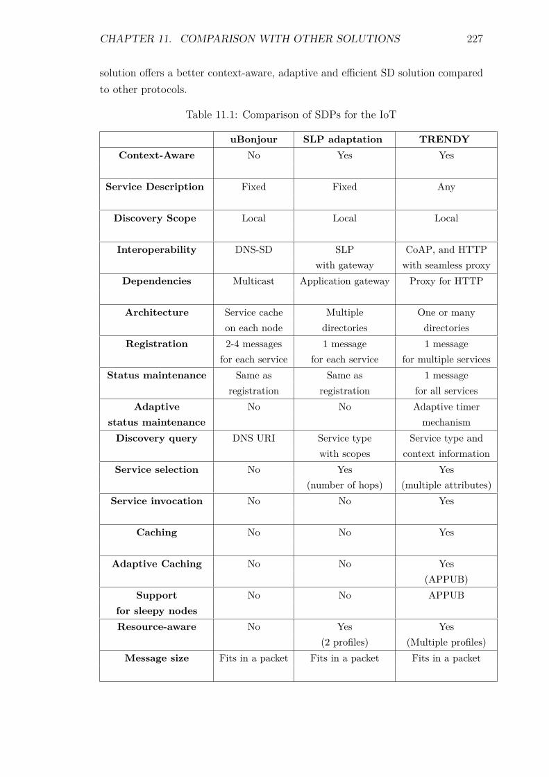
CHAPTER 11. COMPARISON WITH OTHER SOLUTIONS 227
solution offers a better context-aware, adaptive and efficient SD solution comparedto other protocols.
Table 11.1: Comparison of SDPs for the IoT
uBonjour SLP adaptation TRENDYContext-Aware No Yes Yes
Service Description Fixed Fixed Any
Discovery Scope Local Local Local
Interoperability DNS-SD SLP CoAP, and HTTPwith gateway with seamless proxy
Dependencies Multicast Application gateway Proxy for HTTP
Architecture Service cache Multiple One or manyon each node directories directories
Registration 2-4 messages 1 message 1 messagefor each service for each service for multiple services
Status maintenance Same as Same as 1 messageregistration registration for all services
Adaptive No No Adaptive timerstatus maintenance mechanismDiscovery query DNS URI Service type Service type and
with scopes context informationService selection No Yes Yes
(number of hops) (multiple attributes)Service invocation No No Yes
Caching No No Yes
Adaptive Caching No No Yes(APPUB)
Support No No APPUBfor sleepy nodesResource-aware No Yes Yes
(2 profiles) (Multiple profiles)Message size Fits in a packet Fits in a packet Fits in a packet
Chapter 12
Conclusions and Future Work
This research project is focused on providing an efficient, context-aware and adaptiveSD solution for the IoT. In this chapter, the completed work is summarised andthe potential future work is discussed.
12.1 Conclusions
The IoT paradigm has introduced new perspective to be realised for the futureInternet. Isolated islands of WSNs are now enabled to merge with the Internet bynew technologies, such as 6LoWPAN. This merger allows IP based connectivity ofconstrained networks with the Internet. SD and service selection are the key tochange the way we perceive constrained networks. Furthermore, web services canprovide a standard interface to offer interoperability with other existing similarsolutions. However, the design of such a solution faces the underlying challengesof these networks, for example; small packet size and sleep cycles, etc. On onehand, the sleep cycles demand the registry based architecture. On another hand,the limited bandwidth and energy required to decrease the control overhead insuch networks. Services are mostly hosted on battery operated devices, whichare prone to failure. Therefore, status maintenance is required in case of registrybased solution, which increases the bandwidth utilisation and energy consumption.All these challenges require a solution that deals with the heterogeneity andinteroperability requirements of the IoT, while addressing the constraints posed byWSNs.
This research project has proposed TRENDY: an adaptive and context-awareSD solution for the IoT. To deal with the interoperability, this solution employsCoAP-based RESTful web services, which enable application-layer integrationof constrained domains and the Internet. Moreover, the context-aware serviceselection mechanism assists users to discover appropriate services by using available
228
CHAPTER 12. CONCLUSIONS AND FUTURE WORK 229
user- and network-based context. The accuracy of service information is ensuredby keeping soft values at the DA and maintaining the status maintenance.
The trade-off between status maintenance load and reliability is managed by ademand-based adaptive timer. This timer mechanism is even beneficial in scenarioswhere the basic interval for status updates is an hour or more, as the timer’smaximum counter limit can be configured to increase the interval adaptively. AIoT environment can have peaked usage times where a constrained network caneasily be overwhelmed by the increased demand of its resources.
The research project devises the APPUB technique to deal with such situationsby enabling service hosts to share their load with the resource directory. Therefore,SAs push the cache values of busy services towards the registry, which decreases theservice invocation delay because of the cache-hits. The DA ensures the accuracyof cached information by using the respective cache lifetime values to send onlyvalid cached values.
The proposed context-aware grouping technique divides the network at theapplication layer, by creating location-based groups. This grouping of nodes local-ises the control overhead and provides the base for service composition, localisedaggregation and processing of data. The simulation results show that TRENDY’stechniques decrease the control overhead, energy consumption and service invoca-tion delay. Additionally, the grouping technique considerably decreases the numberof packets towards the sink and thus improves scalability in a multi-hop network.However, the performance of the grouping depends on the congruity between thegrouping and routing topologies.
Following is a brief summary about the features of the proposed solution:
Web Service Paradigm: TRENDY uses a RESTful web service paradigm. En-tities use either CoAP (default) or HTTP (in case the targeted host un-derstands it or DA is acting as a proxy) to define their services and tocommunicate with each other. The use of CoAP/HTTP simple proxy canseamlessly translate requests from both protocols. This blends the real-worlddevices into existing web and enables the WoT paradigm.
Context-awareness: In TRENDY, the DA stores all service and contextualinformation, including service descriptions, location, battery consumed, andregistration time for all registered nodes. Furthermore, it maintains a hitcounter for each service, which is incremented whenever a service is discoveredand selected. The maintained context information is used by the serviceselection and better GL selection mechanisms.
Grouping: Context-aware grouping serves several purposes, including simplelocalisation of status maintenance, execution of group-based queries to offer
CHAPTER 12. CONCLUSIONS AND FUTURE WORK 230
an optional local service repository. It costs in terms of some packet overhead.However, networks can get the benefit in the form of localised communication,which conserves energy. In addition, this enables a DA to compose and offergroup-based services, e.g., to actuate a command in a certain area. Theexperiments (Section 8.8) demonstrate the benefit of grouping in terms ofscalability and energy efficiency, while slightly increasing the control overhead.
Hybrid architecture: Basically, TRENDY has a centralised architecture thatconverges to a distributed one when the DA uses context information togroup GMs.
Service Management: All service records have soft states at the DA, therefore,needs to be updated depending on the reliability and other requirements.TRENDY introduces an adaptive timer to increase or decrease the updateinterval depending on the demand of a service. This marginally decreases thebandwidth by reducing the number of update messages. The experiments(Section 7.5) show that the employment of timer mechanism reduces the con-trol overhead and consequently, improves the energy efficiency and scalabilityof TRENDY.
Service Discovery: The DA determines the matching service from the registryusing the attributes of the UA request. Subsequently, it responds back to theUA by appending the service information (resource’s URL and IP address ofthe host) of one or more matching services in the payload.
Service Selection: A UA can ask for the DA’s assistance in selecting the bestmatching host if multiple prospective hosts are found. In this case, theDA determines the most appropriate service (if multiple services have beendiscovered) using available user and network context information, e.g., battery,hops count, UA location, etc. The simulation experiments (Section 6.5) showthat service selection lowers the service invocation delay while improving theenergy efficiency as well.
Service Invocation: SD is completed when an application gets the response witha service identifier and address of its host. TRENDY, however, enablesservice invocation using a RESTful web service interface and takes a stepahead by defining APPUB an adaptive caching technique. The simulations(Section 9.5) supports the point that APPUB reduces the service invocationdelay closer to the NullRDC performance for ContikiMAC scenarios.

CHAPTER 12. CONCLUSIONS AND FUTURE WORK 231
12.2 Future Work
Following are few dimensions and recommendations based on the discussions fromprevious chapters, which can be consider for potential future work:
Extension to the protocol’s functionality: TRENDY has considered differ-ent aspects of the IoT by offering a context-aware SD solution; however,following aspects can be further investigated to allow a broader applicabilityof the protocol.
• Dynamic Service mashups: The context-awareness of TRENDYenables the DA to understand different aspects of services and devicesin a network. Furthermore, its grouping mechanism changes the DA’sperspective of the network. After grouping the nodes, the DA candisseminate a command in an area by passing one command to allGLs in the area. This platform allows a DA to mashup services tocreate higher-level services. The IoT scenarios (Section 4.2) can bebetter served with service mashups; for example, a user can execute onecommand for the whole area without searching and executing servicesindividually. In addition, the DA can smartly offer related services byusing user’s context details. Therefore, an investigation can be done todefine, implement and analyse an extension to grouping mechanism tocreate service mashups dynamically using user’s and network’s contextinformation.
• Semantic discovery: An investigation to improve context-awarenessby analysing the feasibility to use compact and rich formats to enablesemantics based discovery.
• Adaptability of timer: The adaptability of a timer currently considersthe number of times a node has sent updates and the demand of itsservices. An investigation can consider other attributes e.g., node’senergy etc. to analyse the behaviour of the timer and its efficiency.
• Decision making in APPUB : Currently, SAs solely decide aboutpushing the cache at the DA, this can be changed for some scenariosto find out the impact of pull-based approach where a DA requests forcache values to serve queries.
Expansion of experimental analysis: Several experiments are conducted us-ing different RDC, number of queries and topologies. Following are somerecommendations to investigate and broaden the experiments:
CHAPTER 12. CONCLUSIONS AND FUTURE WORK 232
• RPL configurations and performance: The impact of RPL’s DODAGhas been extensively mentioned in experimental analysis. An investiga-tion to change the RPL’s OF to better suit the network dynamics canbe conducted.
• Different routing protocols: Other routing protocols can be em-ployed to analyse their impact on the performance of TRENDY.
• Mobility: Mobile nodes are common in IoT environments, as localmobile phones can become a part of the network to use its services andalso share their services (hosted sensors) with the registry. Therefore,an investigation to find out TRENDY’s behaviour scenarios can beinvestigated and can be improved.
• Compare multicast: The group queries can benefit from multicasttechnique [97] to execute group based commands. However, multicastis costly so an investigation can be conducted to compare availablemulticast techniques and test their applicability to execute group-basedqueries.
• Large-scale Network: Another perspective could be to design thecollaboration of different small networks to form a large-scale SD sys-tem. Moreover, the solution can be deployed in a real-life scenario tomaterialise the discussed scenarios in Section 4.2.
• Searching in a large-scale network: Another dimension is searchingthe objects on the Internet using a search engine so the importantquestions for a future work in a broader perspective include: howservices offered by one network can be made available to the existingDNS infrastructure or what context or semantic information will berequired to facilitate the user to discover appropriate services using asearch engine (related work [24, 85]).
References
[1] W. Adjie-Winoto, E. Schwartz, H. Balakrishnan, and J. Lilley. The designand implementation of an intentional naming system. In ACM SIGOPSOperating Systems Review, volume 33, pages 186–201. ACM, 1999.
[2] R. Ahmed, R. Boutaba, F. Cuervo, Y. Iraqi, D. Li, N. Limam, J. Xiao,and J. Ziembicki. Service discovery protocols: A comparative study. InProceedings of IM, pages 15–18, 2005.
[3] H. Alex, M. Kumar, and B. Shirazi. Service discovery in wireless and mobilenetworks. Wireless information highways, page 251, 2005.
[4] H. Alex, M. Kumar, and B. Shirazi. Midfusion: An adaptive middlewarefor information fusion in sensor network applications. Information Fusion,9(3):332–343, 2008.
[5] Z.B. Alliance. Zigbee specification. ZigBee document 053474r06, version,1:378, 2006.
[6] Giuseppe Anastasi, Marco Conti, Mario Di Francesco, and Andrea Passarella.Energy conservation in wireless sensor networks: A survey. Ad Hoc Networks,7(3):537–568, 2009.
[7] Fatima Muhammad Anwar, Muhammad Taqi Raza, Seung-Wha Yoo, andKi-Hyung Kim. Enum based service discovery architecture for 6lowpan. InWireless Communications and Networking Conference (WCNC), 2010 IEEE,pages 1–6. IEEE, 2010.
[8] K. Arabshian and H. Schulzrinne. Gloserv: Global service discovery archi-tecture. In Mobile and Ubiquitous Systems: Networking and Services, 2004.MOBIQUITOUS 2004. The First Annual International Conference on, pages319–325. IEEE, 2004.
[9] Ken Arnold, Robert Scheifler, Jim Waldo, Bryan O’Sullivan, and AnnWollrath. Jini Specification. Addison-Wesley Longman Publishing Co.,Inc., 1999.
233
REFERENCES 234
[10] L. Atzori, A. Iera, and G. Morabito. The internet of things: A survey.Computer Networks, 54(15):2787–2805, 2010.
[11] M. Balazinska, H. Balakrishnan, and D. Karger. Ins/twine: A scalable peer-to-peer architecture for intentional resource discovery. Pervasive Computing,pages 149–153, 2002.
[12] SIG Bluetooth. Bluetooth specification version 1.1. Available HTTP:http://www. bluetooth. com, 2001.
[13] Carsten Bormann, Angelo P Castellani, and Zach Shelby. Coap: An applica-tion protocol for billions of tiny internet nodes. Internet Computing, IEEE,16(2):62–67, 2012.
[14] S Bradner, L Conroy, and K Fujiwara. The e. 164 to uniform resourceidentifiers (uri) dynamic delegation discovery system (ddds) application(enum). Internet Request for Comments, vol. RFC, 6116, 2011.
[15] J. Buford, B. Burg, E. Celebi, and P. Frankl. Sleeper: A power-conservingservice discovery protocol. In Mobile and Ubiquitous Systems-Workshops,2006. 3rd Annual International Conference on, pages 1–9. IEEE, 2006.
[16] D. Chakraborty, A. Joshi, Y. Yesha, and T. Finin. Gsd: A novel group-basedservice discovery protocol for manets. In Mobile and Wireless Communica-tions Network, 2002. 4th International Workshop on, pages 140–144. IEEE,2002.
[17] D. Chakraborty, A. Joshi, Y. Yesha, and T. Finin. Toward distributed servicediscovery in pervasive computing environments. Mobile Computing, IEEETransactions on, 5(2):97–112, 2006.
[18] Shafique Ahmad Chaudhry, Won Do Jung, Chaudhary Sajjad Hussain,Ali Hammad Akbar, and Ki-Hyung Kim. A proxy-enabled service discoveryarchitecture to find proximity-based services in 6lowpan. In Embedded andUbiquitous Computing, pages 956–965. Springer, 2006.
[19] S.H. Chauhdary, M.Y. Cui, J.H. Kim, A.K. Bashir, and M.S. Park. A context-aware service discovery consideration in 6lowpan. In Third 2008 InternationalConference on Convergence and Hybrid Information Technology, pages 21–26.IEEE, 2008.
[20] Y. Chen and Q. Zhao. On the lifetime of wireless sensor networks. Commu-nications Letters, IEEE, 9(11):976–978, 2005.
REFERENCES 235
[21] S. Cheshire and M. Krochmal. Multicast dns. Technical report, IETF, 2006.
[22] C. Cho and D. Lee. Survey of service discovery architectures for mobile adhoc networks. term paper, Mobile Computing, CEN, 5531, 2005.
[23] E. Christensen, F. Curbera, G. Meredith, S. Weerawarana, et al. Web servicesdescription language (wsdl) 1.1, 2001.
[24] Benoit Christophe, Vincent Verdot, and Vincent Toubiana. Searching the’webof things’. In Semantic Computing (ICSC), 2011 Fifth IEEE InternationalConference on, pages 308–315. IEEE, 2011.
[25] Walter Colitti, Kris Steenhaut, Niccolò De Caro, Bogdan Buta, and VirgilDobrota. Evaluation of constrained application protocol for wireless sensornetworks. In Local & Metropolitan Area Networks (LANMAN), 2011 18thIEEE Workshop on, pages 1–6. IEEE, 2011.
[26] J. Coutaz, J.L. Crowley, S. Dobson, and D. Garlan. Context is key. Commu-nications of the ACM, 48(3):49–53, 2005.
[27] F. Curbera, M. Duftler, R. Khalaf, W. Nagy, N. Mukhi, and S. Weerawarana.Unraveling the web services web: an introduction to soap, wsdl, and uddi.Internet Computing, IEEE, 6(2):86–93, 2002.
[28] A.K. Dey. Understanding and using context. Personal and ubiquitouscomputing, 5(1):4–7, 2001.
[29] A. Dunkels. Full tcp/ip for 8-bit architectures. In Proceedings of the 1stinternational conference on Mobile systems, applications and services, pages85–98. ACM, 2003.
[30] A. Dunkels, J. Alonso, and T. Voigt. Making tcp/ip viable for wireless sensornetworks. SICS Research Report, 2003.
[31] A. Dunkels, B. Gronvall, and T. Voigt. Contiki-a lightweight and flexibleoperating system for tiny networked sensors. In Local Computer Networks,2004. 29th Annual IEEE International Conference on, pages 455–462. IEEE,2004.
[32] Adam Dunkels. The contikimac radio duty cycling protocol. Technical ReportT2011:13, Swedish Institute of Computer Science, 2011.
[33] Adam Dunkels, Fredrik Osterlind, Nicolas Tsiftes, and Zhitao He. Software-based on-line energy estimation for sensor nodes. In Proceedings of the 4thworkshop on Embedded networked sensors, pages 28–32. ACM, 2007.
REFERENCES 236
[34] P.E. Engelstad, Y. Zheng, R. Koodli, and C.E. Perkins. Service discoveryarchitectures for on-demand ad hoc networks. International Journal of AdHoc and Sensor Networks, 1(3), 2005.
[35] Muhammad Omer Farooq and Thomas Kunz. Operating systems for wirelesssensor networks: a survey. Sensors, 11(6):5900–5930, 2011.
[36] Roy Thomas Fielding. Architectural styles and the design of network-basedsoftware architectures. PhD thesis, University of California, 2000.
[37] J. Gao and P. Steenkiste. Rendezvous points-based scalable content discoverywith load balancing. Proceedings of NGC 2002, 2002.
[38] J.A. Garcia-Macias and D.A. Torres. Service discovery in mobile ad-hocnetworks: better at the network layer? In Parallel Processing, 2005. ICPP2005 Workshops. International Conference Workshops on, pages 452–457.IEEE, 2005.
[39] R.S. Gopinath, I. Khan, and Z. Suryady. Optimized web service architecturefor 6lowpan. In Information Networking, 2009. ICOIN 2009. InternationalConference on, pages 1–3. IEEE, 2009.
[40] IETF Zeroconf Working Group et al. Zero configuration networking (zero-conf).
[41] M. Gudgin, N. Mendelsohn, M. Nottingham, and H. Ruellan. Xml-binaryoptimized packaging. W3C Recommendation, Jan, 2005.
[42] Dominique Guinard. A Web of Things Application Architecture – Integratingthe Real-World into the Web. Ph.d., ETH Zurich, 2011.
[43] Dominique Guinard and Vlad Trifa. Towards the web of things: Web mashupsfor embedded devices. In Workshop on Mashups, Enterprise Mashups andLightweight Composition on the Web (MEM 2009), in proceedings of WWW(International World Wide Web Conferences), Madrid, Spain, 2009.
[44] Dominique Guinard, Vlad Trifa, Stamatis Karnouskos, Patrik Spiess, andDomnic Savio. Interacting with the soa-based internet of things: Discovery,query, selection, and on-demand provisioning of web services. ServicesComputing, IEEE Transactions on, 3(3):223–235, 2010.
[45] Dominique Guinard, Vlad Trifa, Friedemann Mattern, and Erik Wilde. Fromthe internet of things to the web of things: Resource-oriented architectureand best practices. In Architecting the Internet of Things, pages 97–129.Springer, 2011.
REFERENCES 237
[46] E. Guttman. Service templates and service: Schemes. Technical report,IETF, 1999.
[47] E. Guttman, C. Perkins, J. Veizades, and M. Day. Slpv2: Service locationprotocol. Technical report, Version 2. RFC 2608, Jun, 1999.
[48] G. Halkes, A. Baggio, and K. Langendoen. A simulation study of integratedservice discovery. Smart Sensing and Context, pages 39–53, 2006.
[49] H. Hassanein, Y. Yang, and A. Mawji. A new approach to service discovery inwireless mobile ad hoc networks. International Journal of Sensor Networks,2(1):135–145, 2007.
[50] S. Helal, N. Desai, V. Verma, and C. Lee. Konark-a service discovery anddelivery protocol for ad-hoc networks. In Wireless Communications andNetworking, 2003. WCNC 2003. 2003 IEEE, volume 3, pages 2107–2113.IEEE, 2003.
[51] A. Helmy, S. Garg, N. Nahata, and P. Pamu. Card: a contact-based archi-tecture for resource discovery in wireless ad hoc networks. Mobile networksand applications, 10(1):99–113, 2005.
[52] Robert M Hinden and Stephen E Deering. Ip version 6 addressing architecture.Technical report, IETF, 2006.
[53] Q. Huaifeng and Z. Xingshe. Context aware sensornet. In Proceedingsof the 3rd international workshop on Middleware for pervasive and ad-hoccomputing, pages 1–7. ACM, 2005.
[54] M.C. Huebscher and J.A. McCann. Adaptive middleware for context-awareapplications in smart-homes. In Proceedings of the 2nd workshop on Middle-ware for pervasive and ad-hoc computing, pages 111–116. ACM, 2004.
[55] J. Hui and P. Thubert. Compression format for ipv6 datagrams in 6lowpannetworks. draft-ietf-6lowpan-hc-04 (work in progress), 2008.
[56] Jonathan W Hui and David E Culler. Ip is dead, long live ip for wirelesssensor networks. In Proceedings of the 6th ACM conference on Embeddednetwork sensor systems, pages 15–28. ACM, 2008.
[57] Bret Hull, Kyle Jamieson, and Hari Balakrishnan. Mitigating congestion inwireless sensor networks. In Proceedings of the 2nd international conferenceon Embedded networked sensor systems, pages 134–147. ACM, 2004.
REFERENCES 238
[58] Philipp K Janert. Gnuplot in action: understanding data with graphs. Man-ning Publications Co., 2009.
[59] C. Jardak, E. Meshkova, J. Riihijarvi, K. Rerkrai, and P. Mahonen. Im-plementation and performance evaluation of nanoip protocols: Simplifiedversions of tcp, udp, http and slp for wireless sensor networks. In WirelessCommunications and Networking Conference, 2008. WCNC 2008. IEEE,pages 2474–2479. IEEE, 2008.
[60] Miloš Jevtić, Nikola Zogović, and Goran Dimić. Evaluation of wireless sensornetwork simulators. In Proceedings of the 17th Telecommunications Forum(TELFOR 2009), Belgrade, Serbia, pages 1303–1306, 2009.
[61] Patrick Olivier Kamgueu, Emmanuel Nataf, Thomas Djotio Ndié, and OlivierFestor. Energy-based routing metric for rpl. Rapport de recherche RR-8208,INRIA, Jan 2013.
[62] James Kempf and Jason Goldschmidt. Notification and subscription for slp.Technical report, RFC 3082, March, 2001.
[63] K Kim, S Yoo, H Lee, S Daniel Park, and J Lee. Simple service locationprotocol (sslp) for 6lowpan. drraft-daniel-6lowpan-sslp-00, 7, 2005.
[64] Ronny Klauck and Michael Kirsche. Bonjour contiki: a case study of adns-based discovery service for the internet of things. In Ad-hoc, Mobile, andWireless Networks, pages 316–329. Springer, 2012.
[65] Ronny Klauck and Michael Kirsche. Enhanced dns message compressionÂŋoptimizing mdns/dnsÂŋsd for the use in 6lowpans. In Proceedings of the9th International Workshop on Sensor Networks and Systems for PervasiveNetworks (PerSeNS 2013), co-located with the 11th IEEE InternationalConference on Pervasive Computing and Communications (PerCom 2013),March 2013.
[66] M. Klein, B. König-Ries, and P. Obreiter. Lanes: A Lightweigth Overlay forService Discorvery in Mobile Ad Hoc Networks. Univ., Fak. für Informatik,2003.
[67] M. Klein, B. Konig-Ries, and P. Obreiter. Service rings-a semantic overlayfor service discovery in ad hoc networks. In Database and Expert SystemsApplications, 2003. Proceedings. 14th International Workshop on, pages 180–185. IEEE, 2003.
REFERENCES 239
[68] R. Koodli and C.E. Perkins. Service discovery in on-demand ad hoc networks.IETF draft, 2002.
[69] Aleksandar Kovacevic, Junaid Ansari, and Petri Mahonen. Nanosd: Aflexible service discovery protocol for dynamic and heterogeneous wirelesssensor networks. In Mobile Ad-hoc and Sensor Networks (MSN), 2010 SixthInternational Conference on, pages 14–19. IEEE, 2010.
[70] Matthias Kovatsch, Simon Duquennoy, and Adam Dunkels. A low-powercoap for contiki. In Mobile Adhoc and Sensor Systems (MASS), 2011 IEEE8th International Conference on, pages 855–860. IEEE, 2011.
[71] M. Krochmal and S. Cheshire. Dns-based service discovery. Technical report,IETF, 2011.
[72] Philip Alexander Levis, Neil Patel, David Culler, and Scott Shenker. Trickle:A self regulating algorithm for code propagation and maintenance in wirelesssensor networks. Computer Science Division, University of California, 2003.
[73] Y. Liang, X. Zhou, Z. Yu, H. Wang, and B. Guo. A context-aware resourcemanagement framework for smart homes. In Ubiquitous Information Techno-logies and Applications (CUTE), 2010 Proceedings of the 5th InternationalConference on, pages 1–8. IEEE, 2010.
[74] H. Luo and M. Barbeau. Performance evaluation of service discovery strategiesin ad hoc networks. In Communication Networks and Services Research,2004. Proceedings. Second Annual Conference on, pages 61–68. IEEE, 2004.
[75] W. Ma, B. Wu, W. Zhang, and L. Cheng. Implementation of a lightweightservice advertisement and discovery protocol for mobile ad hoc networks. InIEEE Globecom, pages 1–5. Citeseer, 2003.
[76] X. Ma and W. Luo. The analysis of 6lowpan technology. In Computa-tional Intelligence and Industrial Application, 2008. PACIIA’08. Pacific-AsiaWorkshop on, volume 1, pages 963–966. IEEE, 2008.
[77] S. Madden, W. Hong, J. Hellerstein, and M. Franklin. TinydbâĂŤa declarativedatabase for sensor networks. TinyDB web page. http://telegraph. cs. berkeley.edu/tinydb, 2005.
[78] R. Marin-Perianu, C. Lombriser, P. Havinga, H. Scholten, and G. Tröster.Tandem: A context-aware method for spontaneous clustering of dynamicwireless sensor nodes. In Proceedings of the 1st international conference onThe internet of things, pages 341–359. Springer-Verlag, 2008.
REFERENCES 240
[79] R. S. Marin-Perianu, P. H. Hartel, and J. Scholten. A classification of servicediscovery protocols. Technical Report TR-CTIT-05-25, Centre for Telematicsand Information Technology University of Twente, Enschede, June 2005.
[80] R. S. Marin-Perianu, J. Scholten, P. J. M. Havinga, and P. H. Hartel.Performance evaluation of a cluster-based service discovery protocol forheterogeneous wireless sensor networks. Technical Report TR-CTIT-06-61,Centre for Telematics and Information Technology University of Twente,Enschede, October 2006.
[81] Raluca Marin-Perianu, Hans Scholten, Paul Havinga, and Pieter Hartel.Energy-efficient cluster-based service discovery in wireless sensor networks.In Local Computer Networks, Proceedings 2006 31st IEEE Conference on,pages 931–938. IEEE, 2006.
[82] RS Marin-Perianu, J. Scholten, PJM Havinga, and PH Hartel. Cluster-basedservice discovery for heterogeneous wireless sensor networks. InternationalJournal of Parallel, Emergent and Distributed Systems, 23(4):325–346, 2008.
[83] B. Martin and B. Jano. Wap binary xml content format. W3C Note, 64,1999.
[84] Simon Mayer and Dominique Guinard. An extensible discovery service forsmart things. In Proceedings of the Second International Workshop on Webof Things, page 7. ACM, 2011.
[85] Simon Mayer, Dominique Guinard, and Vlad Trifa. Searching in a web-based infrastructure for smart things. In Internet of Things (IOT), 2012 3rdInternational Conference on the, pages 119–126. IEEE, 2012.
[86] M. Mealling and R. Daniel. Rfc 2915: The naming authority pointer (naptr)dns resource record, 2000.
[87] E. Meshkova, J. Riihijarvi, M. Petrova, and P. Mahonen. A survey onresource discovery mechanisms, peer-to-peer and service discovery frameworks.Computer Networks, 52(11):2097–2128, 2008.
[88] Adnan Noor Mian, Roberto Baldoni, and Roberto Beraldi. A survey ofservice discovery protocols in multihop mobile ad hoc networks. PervasiveComputing, IEEE, 8(1):66–74, 2009.
[89] G. Montenegro, N. Kushalnagar, J. Hui, and D. Culler. Ipv6 over low-powerwireless personal area networks (6lowpans): Overview, assumptions, problemstatement, and goals. Network working group, IETF, 2007.
REFERENCES 241
[90] G. Montenegro, N. Kushalnagar, J. Hui, and D. Culler. Transmission of ipv6packets over ieee 802.15. 4 networks. Internet proposed standard RFC, 4944,2007.
[91] G. Moritz, E. Zeeb, F. Golatowski, D. Timmermann, and R. Stoll. Webservices to improve interoperability of home healthcare devices. In PervasiveComputing Technologies for Healthcare, 2009. PervasiveHealth 2009. 3rdInternational Conference on, pages 1–4. IEEE, 2009.
[92] G. Moritz, E. Zeeb, S. Pruter, F. Golatowski, D. Timmermann, and R. Stoll.Devices profile for web services in wireless sensor networks: Adaptationsand enhancements. In Emerging Technologies & Factory Automation, 2009.ETFA 2009. IEEE Conference on, pages 1–8. IEEE, 2009.
[93] G. Mulligan. The 6lowpan architecture. In Proceedings of the 4th workshopon Embedded networked sensors, pages 78–82. ACM, 2007.
[94] S.A. Munir, X. Dongliang, C. Canfeng, and J. Ma. Virtual overlay for serviceclassification & discovery in wireless sensor networks. In Advanced Commu-nication Technology, 2009. ICACT 2009. 11th International Conference on,volume 2, pages 991–996. IEEE, 2009.
[95] M. Nidd. Service discovery in deapspace. Personal Communications, IEEE,8(4):39–45, 2001.
[96] D. Noh and H. Shin. Spiz: an effective service discovery protocol for mobilead hoc networks. EURASIP Journal on Wireless Communications andNetworking, 2007(1):27–27, 2007.
[97] George Oikonomou, Iain Phillips, and Theo Tryfonas. Ipv6 multicast forward-ing in rpl-based wireless sensor networks. Wireless Personal Communications,pages 1–28, 2013.
[98] Angela Orebaugh, Gilbert Ramirez, Josh Burke, and Larry Pesce. Wireshark& Ethereal Network Protocol Analyzer Toolkit (Jay Beale’s Open SourceSecurity). Syngress Publishing, 2006.
[99] Fredrik Osterlind, Adam Dunkels, Joakim Eriksson, Niclas Finne, and ThiemoVoigt. Cross-level sensor network simulation with cooja. In Local ComputerNetworks, Proceedings 2006 31st IEEE Conference on, pages 641–648. IEEE,2006.
REFERENCES 242
[100] Charith Perera, Arkady B. Zaslavsky, Peter Christen, and Dimitrios Geor-gakopoulos. Context aware computing for the internet of things: A survey.CoRR, abs/1305.0982, 2013.
[101] S Pohlsen, Carsten Buschmann, and Christian Werner. Integrating a decent-ralized web service discovery system into the internet infrastructure. In onWeb Services, 2008. ECOWS’08. IEEE Sixth European Conference, pages13–20. IEEE, 2008.
[102] M. Presser, P.M. Barnaghi, M. Eurich, and C. Villalonga. The sensei project:integrating the physical world with the digital world of the network of thefuture. Communications Magazine, IEEE, 47(4):1–4, 2009.
[103] S. Ratnasamy, P. Francis, M. Handley, R. Karp, and S. Shenker. A scalablecontent-addressable network. ACM SIGCOMM Computer CommunicationReview, 31(4):161–172, 2001.
[104] M.T. Raza, S.W. Yoo, K.H. Kim, S.S. Joo, and W.C. Jeong. Design andimplementation of an architectural framework for web portals in a ubiquitouspervasive environment. Sensors, 9(7):5201–5223, 2009.
[105] G.G. Richard III. Service advertisement and discovery: enabling universaldevice cooperation. Internet Computing, IEEE, 4(5):18–26, 2000.
[106] F. Sailhan and V. Issarny. Scalable service discovery for manet. In Per-vasive Computing and Communications, 2005. PerCom 2005. Third IEEEInternational Conference on, pages 235–244. IEEE, 2005.
[107] D. Sathan, A. Meetoo, and RK Subramaniam. Context aware lightweightenergy efficient framework. World Academy of Science, Engineering andTechnology, 52, 2009.
[108] G. Schiele, C. Becker, and K. Rothermel. Energy-efficient cluster-based servicediscovery for ubiquitous computing. In Proceedings of the 11th workshop onACM SIGOPS European workshop, page 14. ACM, 2004.
[109] J. Schneider and T. Kamiya. Efficient xml interchange (exi) format 1.0. W3CWorking Draft, 19, 2008.
[110] X. Shao, L.H. Ngoh, T.K. Lee, T.Y. Chai, L. Zhou, and J.C.M. Teo. Multipathcross-layer service discovery (mcsd) for mobile ad hoc networks. In ServicesComputing Conference, 2009. APSCC 2009. IEEE Asia-Pacific, pages 408–413. IEEE, 2009.

REFERENCES 243
[111] Z Shelby. Core link format. draft-ietf-core-link-format-07 (work in progress),2011.
[112] Z. Shelby and C. Bormann. 6LoWPAN: the wireless embedded internet,volume 33. Wiley, 2010.
[113] Z Shelby and S Krco. Core resource directory, draft-shelby-core-resource-directory-02. IETF work in progress, 2012.
[114] Zach Shelby. Embedded web services. Wireless Communications, IEEE,17(6):52–57, 2010.
[115] Tmote Sky. Tmote sky: Ultra low power ieee 802.15.4 compliant wirelesssensor module. Datasheet, Moteiv Corporation, 2006.
[116] A. Sleman and R. Moeller. Integration of wireless sensor network servicesinto other home and industrial networks; using device profile for web services(dpws). In Information and Communication Technologies: From Theory toApplications, 2008. ICTTA 2008. 3rd International Conference on, pages1–5. Ieee, 2008.
[117] P. Spiess, S. Karnouskos, D. Guinard, D. Savio, O. Baecker, L. Souza, andV. Trifa. Soa-based integration of the internet of things in enterprise services.In Web Services, 2009. ICWS 2009. IEEE International Conference on, pages968–975. IEEE, 2009.
[118] D. Steinberg and S. Cheshire. Zero configuration networking: the definitiveguide. O’Reilly Media, Inc., 2005.
[119] V. Stirbu. Towards a restful plug and play experience in the web of things. InSemantic computing, 2008 IEEE international conference on, pages 512–517.IEEE, 2008.
[120] Harsh Sundani, Haoyue Li, Vijay K Devabhaktuni, Mansoor Alam, and PrabirBhattacharya. Wireless sensor network simulators a survey and comparisons.International Journal of Computer Networks (IJCN), 2(6):249–265, 2011.
[121] Vasughi Sundramoorthy. At home in service discovery. University of Twente,2006.
[122] Pascal Thubert. Objective function zero for the routing protocol for low-powerand lossy networks (rpl). Technical Report RFC 6552, IETF, 2012.
[123] A. Varshavsky, B. Reid, and E. de Lara. The need for cross-layer servicediscovery in manets. Report CSRG-492, UofT Computer Science, 2004.
REFERENCES 244
[124] A. Varshavsky, B. Reid, and E. de Lara. A cross-layer approach to servicediscovery and selection in manets. In Mobile Adhoc and Sensor SystemsConference, 2005. IEEE International Conference on, pages 8–pp. IEEE,2005.
[125] J Vasseur, M Kim, K Pister, N Dejean, and D Barthel. Routing metricsused for path calculation in low power and lossy networks. Technical report,IETF, 2011.
[126] Ovidiu Vermesan, Peter Friess, Patrick Guillemin, Sergio Gusmeroli, HaraldSundmaeker, Alessandro Bassi, Ignacio Soler Jubert, Margaretha Mazura,Mark Harrison, M Eisenhauer, et al. Internet of things strategic researchroadmap. Internet of Things-Global Technological and Societal Trends, pages9–52, 2011.
[127] C.N. Ververidis and G.C. Polyzos. Extended zrp: a routing layer based servicediscovery protocol for mobile ad hoc networks. In Mobile and UbiquitousSystems: Networking and Services, 2005. MobiQuitous 2005. The SecondAnnual International Conference on, pages 65–72. IEEE, 2005.
[128] C.N. Ververidis and G.C. Polyzos. Avert: Adaptive service and route discoveryprotocol for manets. In Networking and Communications, 2008. WIMOB’08.IEEE International Conference on Wireless and Mobile Computing,, pages38–43. IEEE, 2008.
[129] C.N. Ververidis and G.C. Polyzos. Service discovery for mobile ad hocnetworks: A survey of issues and techniques. Communications Surveys &Tutorials, IEEE, 10(3):30–45, 2008.
[130] Qiang Wei and Zhi Jin. Service discovery for internet of things: a context-awareness perspective. In Proceedings of the Fourth Asia-Pacific Symposiumon Internetware, page 25. ACM, 2012.
[131] Mark Weiser. The computer for the 21st century. Scientific American,265(3):94–104, 1991.
[132] Erik Wilde. Putting things to REST. Technical Report 2007-015, School ofInformation, UC Berkeley, Berkeley, California, November 2007.
[133] T Winter, ABP Thubert, and et al. Clausen. Rpl: Ipv6 routing protocol forlow-power and lossy networks. Technical Report RFC 6550, IETF, 2012.
[134] M.A. Wister and D.A. Torres. Lift: An efficient cross-layer service discoveryprotocol in manet. In Advanced Information Networking and Applications
REFERENCES 245
Workshops, 2009. WAINA’09. International Conference on, pages 781–786.IEEE, 2009.
[135] A. Wood, J. Stankovic, G. Virone, L. Selavo, Z. He, Q. Cao, T. Doan, Y. Wu,L. Fang, and R. Stoleru. Context-aware wireless sensor networks for assistedliving and residential monitoring. Network, IEEE, 22(4):26–33, 2008.
[136] D. Zeng, S. Guo, and Z. Cheng. The web of things: A survey. Journal ofCommunications, 6(6):424–438, 2011.
[137] B. Zhao, J. Kubiatowicz, and A. Joseph. Tapestry: An infrastructure forfault-tolerant wide-area location and routing. Technical Report UCB/CSD-01-1141, Computer Science Division, U. C. Berkeley, April 2001.
[138] F. Zhu, M. Mutka, and L. Ni. Splendor: A secure, private, and location-aware service discovery protocol supporting mobile services. In PervasiveComputing and Communications, 2003.(PerCom 2003). Proceedings of theFirst IEEE International Conference on, pages 235–242. IEEE, 2003.
[139] Fen Zhu, Matt W Mutka, and Lionel M Ni. Service discovery in pervasivecomputing environments. Pervasive Computing, IEEE, 4(4):81–90, 2005.

Appendices
246
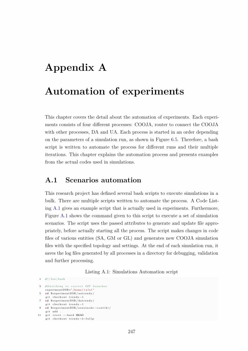
Appendix A
Automation of experiments
This chapter covers the detail about the automation of experiments. Each experi-ments consists of four different processes: COOJA, router to connect the COOJAwith other processes, DA and UA. Each process is started in an order dependingon the parameters of a simulation run, as shown in Figure 6.5. Therefore, a bashscript is written to automate the process for different runs and their multipleiterations. This chapter explains the automation process and presents examplesfrom the actual codes used in simulations.
A.1 Scenarios automation
This research project has defined several bash scripts to execute simulations in abulk. There are multiple scripts written to automate the process. A Code List-ing A.1 gives an example script that is actually used in experiments. Furthermore,Figure A.1 shows the command given to this script to execute a set of simulationscenarios. The script uses the passed attributes to generate and update file appro-priately, before actually starting all the process. The script makes changes in codefiles of various entities (SA, GM or GL) and generates new COOJA simulationfiles with the specified topology and settings. At the end of each simulation run, itsaves the log files generated by all processes in a directory for debugging, validationand further processing.
Listing A.1: Simulations Automation script1 #! / bin / bash
3 #Swicthing to c o r r e c t GIT branchesexperimentDIR=" /home/ t a l a l "
5 cd $experimentDIR / uatrendy /g i t checkout trendy −1
7 cd $experimentDIR / datrendy /g i t checkout trendy −1
9 cd $experimentDIR / sens inode −c o n t i k i /g i t add .
11 g i t r e s e t −−hard HEADg i t checkout trendy −1− f u l l p
247
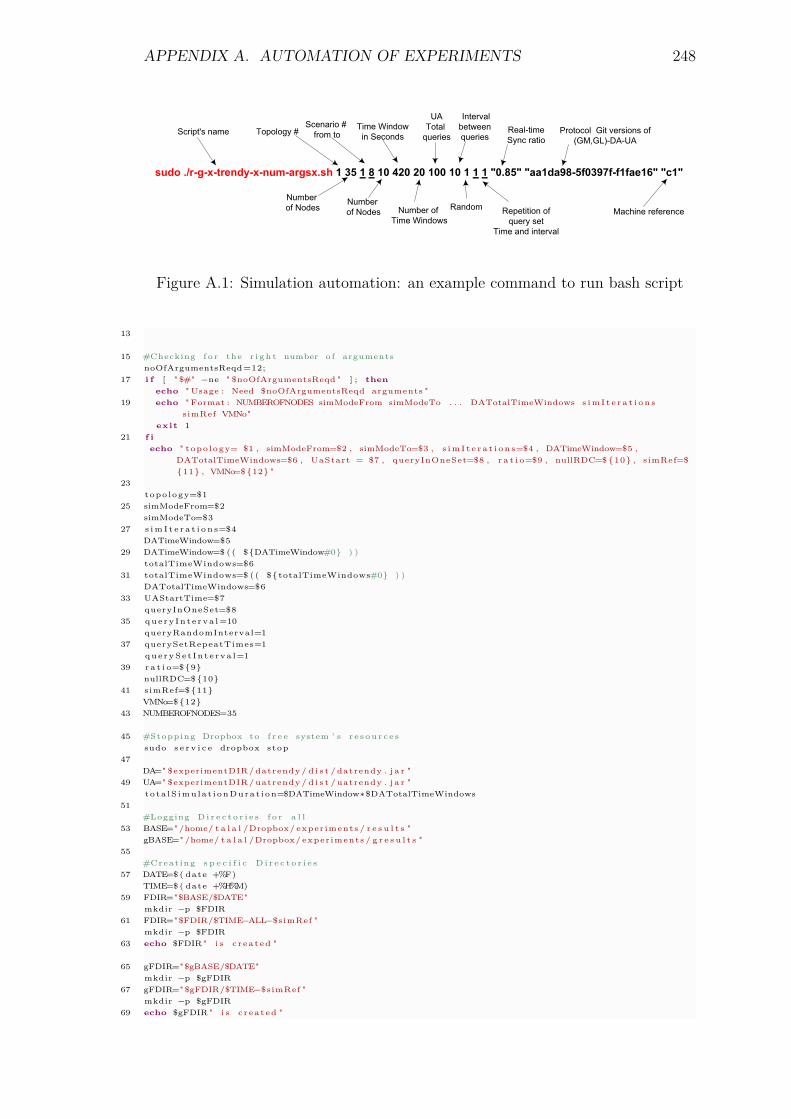
APPENDIX A. AUTOMATION OF EXPERIMENTS 248
���� ��������� ���� ��������� � �� � � �� ��� �� ��� �� � � � ������ ������������������������� ����
������� ����
� ������ ���� �������� �� ������ ���� ��
������� ���� ������ �
���� ������
���� ������� �� ���
��������������
����������������������
��������� ������ ���
���� �� ��������
����
���!������� �����
"���� �� #�� �������� �$#%&#'(!)�!��
%� *��� ������ �
Figure A.1: Simulation automation: an example command to run bash script
13
15 #Checking f o r the r i g h t number o f argumentsnoOfArgumentsReqd =12;
17 i f [ " $#" −ne " $noOfArgumentsReqd " ] ; thenecho " Usage : Need $noOfArgumentsReqd arguments "
19 echo " Format : NUMBEROFNODES simModeFrom simModeTo . . . DATotalTimeWindows s i m I t e r a t i o n ssimRef VMNo"
exit 121 f i
echo " t o p o l o g y= $1 , simModeFrom=$2 , simModeTo=$3 , s i m I t e r a t i o n s=$4 , DATimeWindow=$5 ,DATotalTimeWindows=$6 , UaStart = $7 , queryInOneSet=$8 , r a t i o=$9 , nullRDC=$ {10} , simRef=${11} , VMNo=$ {12} "
23t o p o l o g y=$1
25 simModeFrom=$2simModeTo=$3
27 s i m I t e r a t i o n s=$4DATimeWindow=$5
29 DATimeWindow=$ ( ( ${DATimeWindow#0} ) )totalTimeWindows=$6
31 totalTimeWindows=$ ( ( ${totalTimeWindows#0} ) )DATotalTimeWindows=$6
33 UAStartTime=$7queryInOneSet=$8
35 q u e r y I n t e r v a l =10queryRandomInterval=1
37 querySetRepeatTimes=1q u e r y S e t I n t e r v a l=1
39 r a t i o=${9}nullRDC=$ {10}
41 simRef=$ {11}VMNo=$ {12}
43 NUMBEROFNODES=35
45 #Stopping Dropbox to f r e e system ’ s r e s o u r c e ssudo s e r v i c e dropbox stop
47DA=" $experimentDIR / datrendy / d i s t / datrendy . j a r "
49 UA=" $experimentDIR / uatrendy / d i s t / uatrendy . j a r "t o t a l S i m u l a t i o n D u r a t i o n=$DATimeWindow∗$DATotalTimeWindows
51#Logging D i r e c t o r i e s f o r a l l
53 BASE=" /home/ t a l a l /Dropbox/ exper iments / r e s u l t s "gBASE=" /home/ t a l a l /Dropbox/ exper iments / g r e s u l t s "
55#Creat ing s p e c i f i c D i r e c t o r i e s
57 DATE=$ ( date +%F)TIME=$ ( date +%H%M)
59 FDIR="$BASE/$DATE"mkdir −p $FDIR
61 FDIR="$FDIR/$TIME−ALL−$simRef "mkdir −p $FDIR
63 echo $FDIR" i s c r e a t e d "
65 gFDIR="$gBASE/$DATE"mkdir −p $gFDIR
67 gFDIR=" $gFDIR/$TIME−$simRef "mkdir −p $gFDIR
69 echo $gFDIR " i s c r e a t e d "
APPENDIX A. AUTOMATION OF EXPERIMENTS 249
71GDIR=" $gFDIR/ALL−$NUMBEROFNODES−top$topology −tw$totalTimeWindows−q$queryInOneSet−
r$queryRandomInterval−n$querySetRepeatTimes−f o r −$ s i m I t e r a t i o n s −[$VMNo] "73 mkdir −p $GDIR
echo $GDIR" i s c r e a t e d f o r S i mu la t i o n r e c o r d "75
#S e l e c t i n g a s i m u l a t i o n v a r i a t i o n77 for ( ( i = $simModeFrom ; i <= $simModeTo ; i ++)) ; do
79 SIMNAMEFORMATTED=" case−$i−top$topology −tw$totalTimeWindows−q$queryInOneSet−r$queryRandomInterval−n$querySetRepeatTimes "
CONTIKI=" $experimentDIR / sens inode −c o n t i k i "81 timerMin =1;
timerMax =1;83 t imerThreshold =1;
t imerStep =0;85 #S e t t i n g c o n f i g u r a t i o n s f o r each s i m u l a t i o n
case " $ i " i n87 " 0 " )
i s g r o u p i n g =0;89 numOfGLs=0;
DAMode=0;91 appubThreshold=0
; ;93 " 1 " )
i s g r o u p i n g =0;95 numOfGLs=0;
DAMode=1;97 appubThreshold=0
; ;99 " 2 " )
i s g r o u p i n g =1;101 numOfGLs=5;
DAMode=4;103 appubThreshold=0
; ;105 " 3 " )
i s g r o u p i n g =0;107 numOfGLs=0;
DAMode=7;109 appubThreshold=2
; ;111 " 4 " )
i s g r o u p i n g =1;113 numOfGLs=5;
DAMode=8;115 appubThreshold=2
; ;117 ∗)
echo " Ending "119 ; ;
e s a c121
#Random s e e d s f o r d i f f e r e n t number o f i t e r a t i o n s123 for ( ( j = 1 ; j <= $ s i m I t e r a t i o n s ; j++)) ; do
125 case " $ j " i n
127 " 1 " )newrandomseed =1668841902061472829;
129 ; ;" 2 " )
131 newrandomseed = −8020676306221162569;; ;
133 " 3 " )newrandomseed = −5174799744808039206;
135 ; ;" 4 " )
137 newrandomseed =5471226677158381259;; ;
139 " 5 " )newrandomseed =2442086531776532400;
141 ; ;" 6 " )
143 newrandomseed = −52470407069163422;; ;
145 " 7 " )newrandomseed = −290209011825205304;
147 ; ;
APPENDIX A. AUTOMATION OF EXPERIMENTS 250
" 8 " )149 newrandomseed = −8489044479846245982;
; ;151 " 9 " )
newrandomseed = −2437497649994250447;153 ; ;
" 10 " )155 newrandomseed =4869737434645930484;
; ;157 ∗)
echo " Ending "159 ; ;
e s a c161
#−−−−−−−−−−−−−−−−COOJA SIMULATION GENERATION−−−−−−−−−−−−−−−−−−−−−163 #Total Nodes and/ or grouping [ S p e c i f i c to Si m ul at io n ]
LOWPAN="$CONTIKI/work/ trendy−gm"165 COOJA="$CONTIKI/ t o o l s / c o o j a / d i s t / c o o j a . j a r "
167 cd $LOWPANh e a d e r F i l e=" sim−header . c o o j a "
169 t o p o l o g y F i l e="$NUMBEROFNODES−" g "−$numOfGLs " g "−$topology . t o p o l o g y "f o o t e r F i l e=" sim−f o o t e r . c o o j a "
171SIMFILE="$NUMBEROFNODES−" g "−$numOfGLs " g "−$topology−grouping . c s c "
173 cat $ h e a d e r F i l e $ t o p o l o g y F i l e $ f o o t e r F i l e > " $SIMFILE "SIMULATION=" $SIMFILE "
175#−−−−−−−−−S e l e c t i n g COOJA SCRIPT−−−−−−−−−−−−
177 s c r i p t F i l e="$NUMBEROFNODES−$DATimeWindow−t$totalTimeWindows . j s "cat "$LOWPAN/ g e n e r a l −sim . j s " > " $ s c r i p t F i l e "
179 echo " $ s c r i p t F i l e f i l e i s c r e a t e d "
181 #−−−−−−−−−Changes i n COOJA SCRIPT f o r c o n f i g u r a t i o n s −−−−−−−−timeout=$ ( ( $DATimeWindow∗$totalTimeWindows ∗1000) )
183 timeoutPlus=$ ( ( $DATimeWindow∗$totalTimeWindows ∗1000+100000) )
185 l i n e t o c h a n g e="MAIN−TIMEOUT"n e w l i n e w i t h c o o j a s c r i p t=" $timeoutPlus "
187 awk −v var1=" $ l i n e t o c h a n g e " −v var2=" $ n e w l i n e w i t h c o o j a s c r i p t " ’{gsub ( var1 , var2 )
189 p r i n t} ’ $LOWPAN/ $ s c r i p t F i l e > temp
191 mv temp $LOWPAN/ $ s c r i p t F i l e
193 l i n e t o c h a n g e="TIME−OUT−FINALIZE"n e w l i n e w i t h c o o j a s c r i p t=" $timeout "
195 awk −v var1=" $ l i n e t o c h a n g e " −v var2=" $ n e w l i n e w i t h c o o j a s c r i p t " ’{gsub ( var1 , var2 )
197 p r i n t} ’ $LOWPAN/ $ s c r i p t F i l e > temp
199 mv temp $LOWPAN/ $ s c r i p t F i l e
201 l i n e t o c h a n g e=" nrNodes = 0 ; "numOfNodesForJS=$ ( ($NUMBEROFNODES+1) )
203 n e w l i n e w i t h c o o j a s c r i p t=" nrNodes = $numOfNodesForJS ; "awk −v var1=" $ l i n e t o c h a n g e " −v var2=" $ n e w l i n e w i t h c o o j a s c r i p t " ’{
205 gsub ( var1 , var2 )p r i n t
207 } ’ $LOWPAN/ $ s c r i p t F i l e > tempmv temp $LOWPAN/ $ s c r i p t F i l e
209l i n e t o c h a n g e=" tota l_reports_needed = 0 ; "
211 numOfNodesForJS=$ ( ($NUMBEROFNODES+1) )n e w l i n e w i t h c o o j a s c r i p t=" total_reports_needed = $NUMBEROFNODES; "
213 awk −v var1=" $ l i n e t o c h a n g e " −v var2=" $ n e w l i n e w i t h c o o j a s c r i p t " ’{gsub ( var1 , var2 )
215 p r i n t} ’ $LOWPAN/ $ s c r i p t F i l e > temp
217 mv temp $LOWPAN/ $ s c r i p t F i l e
219 l i n e t o c h a n g e="RATIO−TO−CHANGE1"n e w l i n e w i t h c o o j a s c r i p t=" $ r a t i o "
221 awk −v var1=" $ l i n e t o c h a n g e " −v var2=" $ n e w l i n e w i t h c o o j a s c r i p t " ’{gsub ( var1 , var2 )
223 p r i n t} ’ $LOWPAN/ $ s c r i p t F i l e > temp
225 mv temp $LOWPAN/ $ s c r i p t F i l e
227 l i n e t o c h a n g e="RATIO−TO−CHANGE2"
APPENDIX A. AUTOMATION OF EXPERIMENTS 251
n e w l i n e w i t h c o o j a s c r i p t=" $ r a t i o "229 awk −v var1=" $ l i n e t o c h a n g e " −v var2=" $ n e w l i n e w i t h c o o j a s c r i p t " ’{
gsub ( var1 , var2 )231 p r i n t
} ’ $LOWPAN/ $ s c r i p t F i l e > temp233 mv temp $LOWPAN/ $ s c r i p t F i l e
235 echo " $ s c r i p t F i l e f i l e i s CHANGED"
237 #−−−−−−−−−−−−−−−−Java s c r i p t f o r COOJA SIMULATION−−−−−−−−−−−−−−−−−−l i n e t o c h a n g e="< s c r i p t f i l e ></ s c r i p t f i l e >"
239 n e w l i n e w i t h c o o j a s c r i p t="< s c r i p t f i l e >[CONTIKI_DIR] / work/ trendy−gm/ $ s c r i p t F i l e </ s c r i p t f i l e >"
241 awk −v var1=" $ l i n e t o c h a n g e " −v var2=" $ n e w l i n e w i t h c o o j a s c r i p t " ’{gsub ( var1 , var2 )
243 p r i n t} ’ $SIMULATION > temp
245 mv temp $SIMULATION
247 #−−−−−−−−−−−−−Changing S im u la t i o n speed−−−−−−−−−−−−−−−−−l i n e t o c h a n g e="<s p e e d l i m i t >0.85</ s p e e d l i m i t >"
249 n e w l i n e w i t h c o o j a s c r i p t="<s p e e d l i m i t >$ r a t i o </s p e e d l i m i t >"awk −v var1=" $ l i n e t o c h a n g e " −v var2=" $ n e w l i n e w i t h c o o j a s c r i p t " ’{
251 gsub ( var1 , var2 )p r i n t
253 } ’ $SIMULATION > tempmv temp $SIMULATION
255#−−−−−−−−−−−−−−−−−−−−−Changes i n o t h e r f i l e s −−−−−−−−−−−−−−−−−−−−−−−
257 workDIR="$CONTIKI/work "SAVEIFS=$IFS
259 IFS=$ ( echo −en " \n\b " )for ( (gm = 1 ; gm <= 5 ; gm++)) ; do
261case "$gm" i n
263" 1 " )
265 gmFile=" $workDIR/ trendy−gm/ group−member . c "; ;
267 " 2 " )gmFile=" $workDIR/ trendy−gm group −2/group−member . c "
269 ; ;" 3 " )
271 gmFile=" $workDIR/ trendy−gm group −3/group−member . c "; ;
273 " 4 " )gmFile=" $workDIR/ trendy−gm group −4/group−member . c "
275 ; ;" 5 " )
277 gmFile=" $workDIR/ trendy−gm group −5/group−member . c "; ;
279 ∗)echo " Ending "
281 ; ;e s a c
283 echo " s e l e c t e d f i l e : $gmFile and APPUB = $appubThreshold "
285 l i n e t o c h a n g e="#d e f i n e hit_count_threshold "n e w l i n e w i t h c o o j a s c r i p t="#d e f i n e hit_count_threshold $appubThreshold "
287 sed − i " s / $ l i n e t o c h a n g e . ∗ / $ n e w l i n e w i t h c o o j a s c r i p t / " $gmFiledone
289IFS=$SAVEIFS
291#−−−−−−−−−−−−−−S e l e c t i o n o f RDC−−−−−−−−−−−−−−−−−−
293 workDIR="$CONTIKI/work "SAVEIFS=$IFS
295 IFS=$ ( echo −en " \n\b " )for ( ( sa = 1 ; sa <= 1 1 ; sa++)) ; do
297case " $sa " i n
299" 1 " )
301 s a F i l e=" $workDIR/ trendy−gm/ p r o j e c t −c o n f . h "; ;
303 " 2 " )s a F i l e=" $workDIR/ trendy−gm group −2/ p r o j e c t −c o n f . h "
305 ; ;" 3 " )
307 s a F i l e=" $workDIR/ trendy−gm group −3/ p r o j e c t −c o n f . h "
APPENDIX A. AUTOMATION OF EXPERIMENTS 252
; ;309 " 4 " )
s a F i l e=" $workDIR/ trendy−gm group −4/ p r o j e c t −c o n f . h "311 ; ;
" 5 " )313 s a F i l e=" $workDIR/ trendy−gm group −5/ p r o j e c t −c o n f . h "
; ;315 " 6 " )
s a F i l e=" $workDIR/ trendy−g l / p r o j e c t −c o n f . h "317 ; ;
" 7 " )319 s a F i l e=" $workDIR/ trendy−g l group −2/ p r o j e c t −c o n f . h "
; ;321 " 8 " )
s a F i l e=" $workDIR/ trendy−g l group −3/ p r o j e c t −c o n f . h "323 ; ;
" 9 " )325 s a F i l e=" $workDIR/ trendy−g l group −4/ p r o j e c t −c o n f . h "
; ;327 " 10 " )
s a F i l e=" $workDIR/ trendy−g l group −5/ p r o j e c t −c o n f . h "329 ; ;
" 11 " )331 s a F i l e="$CONTIKI/ examples / ipv6 / rpl −border−r o u t e r / p r o j e c t −c o n f . h "
; ;333 ∗)
echo " Ending "335 ; ;
e s a c337 echo " s e l e c t e d f i l e : $ s a F i l e and nullRDC = $nullRDC "
339 l i n e t o c h a n g e="#d e f i n e NULLRDC"n e w l i n e w i t h c o o j a s c r i p t="#d e f i n e NULLRDC $nullRDC "
341 sed − i " s / $ l i n e t o c h a n g e . ∗ / $ n e w l i n e w i t h c o o j a s c r i p t / " $ s a F i l edone
343IFS=$SAVEIFS
345#−−−−−−−−−−−−−−Loading new seed v a l u e s i n a s i m u l a t i o n −−−−−−−−−−−−
347 l i n e t o c h a n g e="<randomseed>generated </randomseed>"newlinewithrandomseed="<randomseed>$newrandomseed</randomseed>"
349awk −v var1=" $ l i n e t o c h a n g e " −v var2=" $newlinewithrandomseed " ’{
351 gsub ( var1 , var2 )p r i n t
353 } ’ $SIMULATION > tempmv temp $SIMULATION
355echo $SIMULATION" with random seed = $newrandomseed i s s t a r t i n g "
357#S p e c i f i c to S im ul a t i on
359 SDIR="$FDIR/$NUMBEROFNODES−$SIMNAMEFORMATTED−f o r −$ s i m I t e r a t i o n s −[$VMNo] "mkdir −p $SDIR
361 echo $SDIR " i s c r e a t e d f o r Si m ul at i on r e c o r d "
363 unset DISPLAYcd $LOWPAN
365
367 #Log f i l e f o r Simulation ’ s t e r m i n a l outputLOGFILE=" $SDIR/ sim$j . l o g "
369 echo "GIT ID : $simRef by VM#$VMNo" >>$LOGFILEecho " The S im u la t i on Duration = $ t o t a l S i m u l a t i o n D u r a t i o n " >>$LOGFILE
371 echo " Total Nodes $NUMBEROFNODES" >>$LOGFILEecho " o f $ j th o f $ s i m I t e r a t i o n s i t e r a t i o n s " >>$LOGFILE
373 echo "DA l a s t f o r $DATotalTimeWindows time windows each with $DATimeWindow seconds " >>$LOGFILEecho "UA w i l l query $queryInOneSet q u e r i e s with i n t e r v a l o f $ q u e r y I n t e r v a l seconds " >>$LOGFILE
375 echo "UA w i l l r e p e a t above query s e t f o r $querySetRepeatTimes t imes each with$ q u e r y S e t I n t e r v a l seconds i n t e r v a l " >>$LOGFILE
377 #Cleaning up b e f o r e endingrm ∗ . t e s t l o g
379 rm ∗ . t x trm ∗ . l o g
381 rm ∗ . datrm ∗ . pcap
383#−−−−−−−−−−S t a r t i n g and s c h e d u l i n g p r o c e s s e s −−−−−−−−−−−−−−−−−−−−−−−−−−
385 s l e e p 120 && sudo make connect−rou ter −c o o j a >> $LOGFILE&pid_cooja_router=$ !
APPENDIX A. AUTOMATION OF EXPERIMENTS 253
387 s l e e p $UAStartTime && java −j a r $UA $queryInOneSet $ q u e r y I n t e r v a l $queryRandomInterval$querySetRepeatTimes $ q u e r y S e t I n t e r v a l $ r a t i o >> $LOGFILE&
pid_ua=$ !389
java −j a r $DA $DATimeWindow $DATotalTimeWindows $DAMode $ r a t i o $timerMin $timerMax$timerThreshold $t imerStep >> $LOGFILE&
391 pid_da=$ !/ usr / bin / time −−v e r b o s e −o c o o j a t i m e . l o g −a java −j a r $COOJA −nogui=$SIMULATION −c o n t i k i=
$CONTIKI >> $LOGFILE&393 pid_cooja=$ !
395 wait $pid_cooja
397 s l e e p 10k i l l −9 $pid_ua
399 k i l l −9 $pid_dak i l l −9 $pid_cooja_router
401#General d e t a i l e d l o g
403 cat d a D e t a i l . t x t >> " $SDIR/$SIMNAMEFORMATTED−da−d e t a i l . l o g "cat d a x t r a d e t a i l . t x t >> " $SDIR/$SIMNAMEFORMATTED−d a F u l l D e t a i l . l o g "
405 cat uacompleteLog . t x t >> " $SDIR/$SIMNAMEFORMATTED−ua−d e t a i l . l o g "cat COOJA. t e s t l o g >> " $SDIR/$SIMNAMEFORMATTED−Lowpan−d e t a i l . l o g "
407 cat daperformance . t x t >> " $SDIR/$SIMNAMEFORMATTED−daperformance . l o g "cat uaperformance . t x t >> " $SDIR/$SIMNAMEFORMATTED−uaperformance . l o g "
409 cat uaperformance−p r o c e s s e d . t x t >> " $SDIR/$SIMNAMEFORMATTED−uaperformance−p r o c e s s e d . l o g "cat l−energy−a l l . dat >> " $SDIR/$SIMNAMEFORMATTED−l−energy−a l l . dat "
411 cat l−energy−ind . dat >> " $SDIR/$SIMNAMEFORMATTED−l−energy−ind . dat "cat l−raw−energy−ind . dat >> " $SDIR/$SIMNAMEFORMATTED−l−raw−energy−ind . dat "
413 cat l−packet−a l l . dat >> " $SDIR/$SIMNAMEFORMATTED−l−packet−a l l . dat "cat l−packet−ind . dat >> " $SDIR/$SIMNAMEFORMATTED−l−packet−ind . dat "
415 cat radio −p a c k e t s . dat >> " $SDIR/$SIMNAMEFORMATTED−radio −p a c k e t s . l o g "cat " r a d i o l o g −" ∗ " . pcap " >> " $SDIR/$SIMNAMEFORMATTED−p a c k e t s . pcap "
417 cat c o o j a t i m e . l o g >> " $SDIR/$SIMNAMEFORMATTED−coojaTime . l o g "
419#Saving Log f o r g e n e r a t i n g graphs
421 cat uaperformance . t x t >> "$GDIR/ case−$i−uaperformance . l o g "cat uaperformance−p r o c e s s e d . t x t >> "$GDIR/ case−$i−uaperformance−p r o c e s s e d . l o g "
423 cat daperformance . t x t >> "$GDIR/ case−$i−daperformance . l o g "cat l−energy−a l l . dat >> "$GDIR/ case−$i−energy−a l l . dat "
425 cat l−energy−ind . dat >> "$GDIR/ case−$i−energy−ind . dat "cat l−raw−energy−ind . dat >> "$GDIR/ case−$i−raw−energy−ind . dat "
427 cat l−packet−a l l . dat >> "$GDIR/ case−$i−packet−a l l . dat "cat l−packet−ind . dat >> "$GDIR/ case−$i−packet−ind . dat "
429 cat radio −p a c k e t s . dat >> "$GDIR/ case−$i−radio −p a c k e t s . l o g "cat " r a d i o l o g −" ∗ " . pcap " >> "$GDIR/ case−$i−p a c k e t s . pcap "
431
433 #Cleaning up b e f o r e endingrm ∗ . t e s t l o g
435 rm ∗ . t x trm ∗ . l o g
437 rm ∗ . datrm ∗ . pcap
439done #End o f m u l t i p l e i t e r a t i o n s o f one Si mu la t io n
441 done #End o f one Unique S i mu la t io n − Loop f o r a l l s i m u l a t i o n ssudo s e r v i c e dropbox s t a r t
A.2 Script for 6LoWPAN data gathering
Each COOJA simulation requires some Javascript to produce results in log fileswith different level of details. This automates the process of result gatheringin a specified format for each experiment, which aids the process of debugging,validation and measurements of different performance metrics for 6LoWPANs.Following is an example of such a Javascript:
1 importPackage ( java . i o ) ;
3 // F u n c t i o n to r e c o r d s t a t i s t i c s a f t e r e a c h t i m e w i n d o w
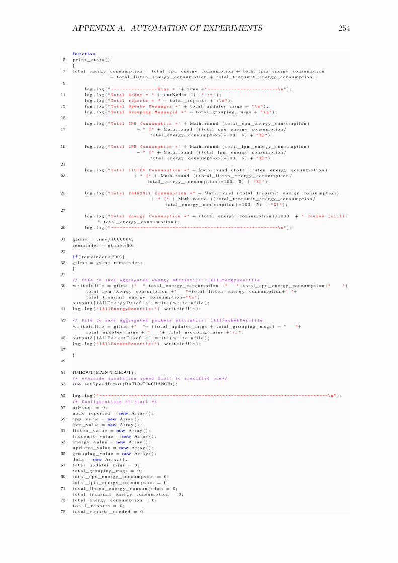
APPENDIX A. AUTOMATION OF EXPERIMENTS 254
function5 p r i n t _ s t a t s ( )
{7 total_energy_consumption = total_cpu_energy_consumption + total_lpm_energy_consumption
+ total_l isten_energy_consumption + total_transmit_energy_consumption ;9
l o g . l o g ( " - - - - - - - - - - - - - - - - T i m e = "+ time +" - - - - - - - - - - - - - - - - - - - - - - - -\ n " ) ;11 l o g . l o g ( " T o t a l N o d e s = " + ( nrNodes −1) +" :\ n " ) ;
l o g . l o g ( " T o t a l r e p o r t s = " + t o t a l _ r e p o r t s +" :\ n " ) ;13 l o g . l o g ( " T o t a l U p d a t e M e s s a g e s = " + total_updates_msgs + " \ n " ) ;
l o g . l o g ( " T o t a l G r o u p i n g M e s s a g e s = " + total_grouping_msgs + " \ n " ) ;15
l o g . l o g ( " T o t a l C P U C o n s u m p t i o n = " + Math . round ( total_cpu_energy_consumption )17 + " [ " + Math . round ( ( total_cpu_energy_consumption /
total_energy_consumption ) ∗100 , 5) + " %] " ) ;
19 l o g . l o g ( " T o t a l L P M C o n s u m p t i o n = " + Math . round ( total_lpm_energy_consumption )+ " [ " + Math . round ( ( total_lpm_energy_consumption /
total_energy_consumption ) ∗100 , 5) + " %] " ) ;21
l o g . l o g ( " T o t a l L I S T E N C o n s u m p t i o n = " + Math . round ( total_l isten_energy_consumption )23 + " [ " + Math . round ( ( total_l isten_energy_consumption /
total_energy_consumption ) ∗100 , 5) + " %] " ) ;
25 l o g . l o g ( " T o t a l T R A N S M I T C o n s u m p t i o n = " + Math . round ( total_transmit_energy_consumption )+ " [ " + Math . round ( ( total_transmit_energy_consumption /
total_energy_consumption ) ∗100 , 5) + " %] " ) ;27
l o g . l o g ( " T o t a l E n e r g y C o n s u m p t i o n = " + ( total_energy_consumption ) /1000 + " J o u l e s [ m i l l i :"+total_energy_consumption ) ;
29 l o g . l o g ( " - - - - - - - - - - - - - - - - - - - - - - - - - - - - - - - - - - - - - - - - - - - - - - - - - - - - - - - - -\ n " ) ;
31 gtime = time /1000000;remainder = gtime %60;
33i f ( remainder <200){
35 gtime = gtime−remainder ;}
37// F i l e to s a v e a g g r e g a t e d e n e r g y s t a t i s t i c s : l A l l E n e r g y D e s c f i l e
39 w r i t e i n f i l e = gtime +" "+total_energy_consumption +" "+total_cpu_energy_consumption+" "+total_lpm_energy_consumption +" "+total_l isten_energy_consumption+" "+total_transmit_energy_consumption+" \ n " ;
output1 [ l A l l E n e r g y D e s c f i l e ] . w r i t e ( w r i t e i n f i l e ) ;41 l o g . l o g ( " l A l l E n e r g y D e s c f i l e : "+ w r i t e i n f i l e ) ;
43 // F i l e to s a v e a g g r e g a t e d p a c k e t s s t a t i s t i c s : l A l l P a c k e t D e s c f i l ew r i t e i n f i l e = gtime +" "+ ( total_updates_msgs + total_grouping_msgs ) + " "+
total_updates_msgs + " "+ total_grouping_msgs +" \ n " ;45 output3 [ l A l l P a c k e t D e s c f i l e ] . w r i t e ( w r i t e i n f i l e ) ;
l o g . l o g ( " l A l l P a c k e t D e s c f i l e : "+ w r i t e i n f i l e ) ;47
}49
51 TIMEOUT(MAIN−TIMEOUT) ;/* o v e r r i d e s i m u l a t i o n s p e e d l i m i t to s p e c i f i e d o n e */
53 sim . setSpeedLimit (RATIO−TO−CHANGE1) ;
55 l o g . l o g ( " - - - - - - - - - - - - - - - - - - - - - - - - - - - - - - - - - - - - - - - - - - - - - - - - - - - - - - - - - - - - - - - - - - - - - - - - - - - - - -\ n " ) ;/* C o n f i g u r a t i o n s at s t a r t */
57 nrNodes = 0 ;node_reported = new Array ( ) ;
59 cpu_value = new Array ( ) ;lpm_value = new Array ( ) ;
61 l i s t e n _ v a l u e = new Array ( ) ;transmit_value = new Array ( ) ;
63 energy_value = new Array ( ) ;updates_value = new Array ( ) ;
65 grouping_value = new Array ( ) ;data = new Array ( ) ;
67 total_updates_msgs = 0 ;total_grouping_msgs = 0 ;
69 total_cpu_energy_consumption = 0 ;total_lpm_energy_consumption = 0 ;
71 total_l isten_energy_consumption = 0 ;total_transmit_energy_consumption = 0 ;
73 total_energy_consumption = 0 ;t o t a l _ r e p o r t s = 0 ;
75 total_reports_needed = 0 ;
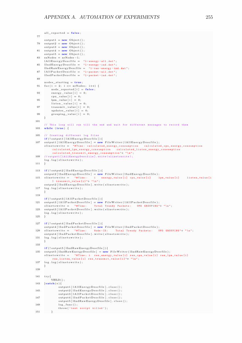
APPENDIX A. AUTOMATION OF EXPERIMENTS 255
a l l _ r e p o r t e d = f a l s e ;77
output1 = new Object ( ) ;79 output2 = new Object ( ) ;
output3 = new Object ( ) ;81 output4 = new Object ( ) ;
output5 = new Object ( ) ;83 saNodes = nrNodes −1;
l A l l E n e r g y D e s c f i l e = " l - e n e r g y - a l l . d a t " ;85 l I n d E n e r g y D e s c f i l e = " l - e n e r g y - i n d . d a t " ;
l IndRawEnergyDescf i le = " l - raw - e n e r g y - i n d . d a t " ;87 l A l l P a c k e t D e s c f i l e = " l - p a c k e t - a l l . d a t " ;
l I n d P a c k e t D e s c f i l e = " l - p a c k e t - i n d . d a t " ;89
n o d e s _ s t a r t i n g = true ;91 f o r ( i = 2 ; i <= nrNodes ; i ++) {
node_reported [ i ] = f a l s e ;93 energy_value [ i ] = 0 ;
cpu_value [ i ] = 0 ;95 lpm_value [ i ] = 0 ;
l i s t e n _ v a l u e [ i ] = 0 ;97 transmit_value [ i ] = 0 ;
updates_value [ i ] = 0 ;99 grouping_value [ i ] = 0 ;
}101
// T h i s l o o p w i l l r u n t i l l t h e e n d a n d w a i t f o r d i f f e r e n t m e s s a g e s to r e c o r d t h e m103 while ( true ) {
105 // C r e a t i n g d i f f e r e n t l o g f i l e si f ( ! output1 [ l A l l E n e r g y D e s c f i l e ] ) {
107 output1 [ l A l l E n e r g y D e s c f i l e ] = new F i l e W r i t e r ( l A l l E n e r g y D e s c f i l e ) ;s l i n e t o w r i t e = " # T i m e : c a l c u l a t e d _ e n e r g y _ c o n s u m p t i o n c a l c u l a t e d _ c p u _ e n e r g y _ c o n s u m p t i o n
c a l c u l a t e d _ l p m _ e n e r g y _ c o n s u m p t i o n c a l c u l a t e d _ l i s t e n _ e n e r g y _ c o n s u m p t i o nc a l c u l a t e d _ t r a n s m i t _ e n e r g y _ c o n s u m p t i o n "+ " \ n " ;
109 // o u t p u t 1 [ l A l l E n e r g y D e s c f i l e ]. w r i t e ( s l i n e t o w r i t e ) ;l o g . l o g ( s l i n e t o w r i t e ) ;
111 }
113 i f ( ! output2 [ l I n d E n e r g y D e s c f i l e ] ) {output2 [ l I n d E n e r g y D e s c f i l e ] = new F i l e W r i t e r ( l I n d E n e r g y D e s c f i l e ) ;
115 s l i n e t o w r i t e = " # T i m e : i e n e r g y _ v a l u e [ i ] c p u _ v a l u e [ i ] l p m _ v a l u e [ i ] l i s t e n _ v a l u e [ i] t r a n s m i t _ v a l u e [ i ] "+ " \ n " ;
output2 [ l I n d E n e r g y D e s c f i l e ] . w r i t e ( s l i n e t o w r i t e ) ;117 l o g . l o g ( s l i n e t o w r i t e ) ;
}119
i f ( ! output3 [ l A l l P a c k e t D e s c f i l e ] ) {121 output3 [ l A l l P a c k e t D e s c f i l e ] = new F i l e W r i t e r ( l A l l P a c k e t D e s c f i l e ) ;
s l i n e t o w r i t e = " # T i m e : T o t a l T r e n d y P a c k e t s : U P D G R O U P I N G "+ " \ n " ;123 output3 [ l A l l P a c k e t D e s c f i l e ] . w r i t e ( s l i n e t o w r i t e ) ;
l o g . l o g ( s l i n e t o w r i t e ) ;125 }
127 i f ( ! output4 [ l I n d P a c k e t D e s c f i l e ] ) {output4 [ l I n d P a c k e t D e s c f i l e ] = new F i l e W r i t e r ( l I n d P a c k e t D e s c f i l e ) ;
129 s l i n e t o w r i t e = " # T i m e : Node - ID : T o t a l T r e n d y P a c k e t s : U P D G R O U P I N G "+ " \ n " ;output4 [ l I n d P a c k e t D e s c f i l e ] . w r i t e ( s l i n e t o w r i t e ) ;
131 l o g . l o g ( s l i n e t o w r i t e ) ;}
133i f ( ! output5 [ l IndRawEnergyDescf i le ] ) {
135 output5 [ l IndRawEnergyDescf i le ] = new F i l e W r i t e r ( l IndRawEnergyDescf i le ) ;s l i n e t o w r i t e = " # T i m e : i r a w _ e n e r g y _ v a l u e [ i ] r a w _ c p u _ v a l u e [ i ] r a w _ l p m _ v a l u e [ i ]
r a w _ l i s t e n _ v a l u e [ i ] r a w _ t r a n s m i t _ v a l u e [ i ] "+ " \ n " ;137 l o g . l o g ( s l i n e t o w r i t e ) ;
}139
141 t r y {YIELD ( ) ;
143 }catch ( e ) {output1 [ l A l l E n e r g y D e s c f i l e ] . c l o s e ( ) ;
145 output2 [ l I n d E n e r g y D e s c f i l e ] . c l o s e ( ) ;output3 [ l A l l P a c k e t D e s c f i l e ] . c l o s e ( ) ;
147 output4 [ l I n d P a c k e t D e s c f i l e ] . c l o s e ( ) ;output5 [ l IndRawEnergyDescf i le ] . c l o s e ( ) ;
149 log_func ( ) ;throw ( ’ t e s t s c r i p t k i l l e d ’ ) ;
151 }
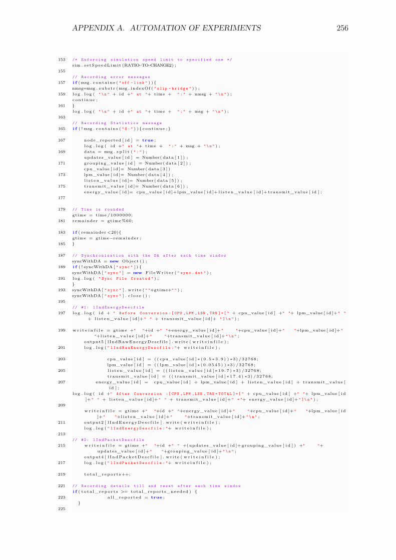
APPENDIX A. AUTOMATION OF EXPERIMENTS 256
153 /* E n f o r c i n g s i m u l a t i o n s p e e d l i m i t to s p e c i f i e d o n e */sim . setSpeedLimit (RATIO−TO−CHANGE2) ;
155// R e c o r d i n g e r r o r m e s s a g e s
157 i f ( msg . c o n t a i n s ( " off - l i n k " ) ) {nmsg=msg . s u b s t r ( msg . indexOf ( " slip - b r i d g e " ) ) ;
159 l o g . l o g ( " \ n " + i d +" at "+ time + " : " + nmsg + " \ n " ) ;c o n t i n u e ;
161 }l o g . l o g ( " \ n " + i d +" at "+ time + " : " + msg + " \ n " ) ;
163// R e c o r d i n g S t a t i s t i c s m e s s a g e
165 i f ( ! msg . c o n t a i n s ( " S : " ) ) { c o n t i n u e ; }
167 node_reported [ i d ] = true ;l o g . l o g ( i d +" at "+ time + " : " + msg + " \ n " ) ;
169 data = msg . s p l i t ( " : " ) ;updates_value [ i d ] = Number ( data [ 1 ] ) ;
171 grouping_value [ i d ] = Number ( data [ 2 ] ) ;cpu_value [ i d ]= Number ( data [ 3 ] )
173 lpm_value [ i d ]= Number ( data [ 4 ] ) ;l i s t e n _ v a l u e [ i d ]= Number ( data [ 5 ] ) ;
175 transmit_value [ i d ]= Number ( data [ 6 ] ) ;energy_value [ i d ]= cpu_value [ i d ]+ lpm_value [ i d ]+ l i s t e n _ v a l u e [ i d ]+ transmit_value [ i d ] ;
177
179 // T i m e is r o u n d e dgtime = time /1000000;
181 remainder = gtime %60;
183 i f ( remainder <20){gtime = gtime−remainder ;
185 }
187 // S y n c h r o n i s a t i o n w i t h t h e DA a f t e r e a c h t i m e w i n d o wsyncWithDA = new Object ( ) ;
189 i f ( ! syncWithDA [ " s y n c " ] ) {syncWithDA [ " s y n c " ] = new F i l e W r i t e r ( " s y n c . d a t " ) ;
191 l o g . l o g ( " S y n c F i l e C r e a t e d " ) ;}
193 syncWithDA [ " s y n c " ] . w r i t e ( " "+gtime+" " ) ;syncWithDA [ " s y n c " ] . c l o s e ( ) ;
195// # 1 : l I n d E n e r g y D e s c f i l e
197 l o g . l o g ( i d + " B e f o r e C o n v e r s i o n :[ CPU , LPM , LSN , T R N ] = [ " + cpu_value [ i d ] +" "+ lpm_value [ i d ]+ " "+ l i s t e n _ v a l u e [ i d ]+ " " + transmit_value [ i d ]+ " ]\ n " ) ;
199 w r i t e i n f i l e = gtime +" "+i d +" "+energy_value [ i d ]+ " "+cpu_value [ i d ]+ " "+lpm_value [ i d ]+ ""+l i s t e n _ v a l u e [ i d ]+ " "+transmit_value [ i d ]+ " \ n " ;
output5 [ l IndRawEnergyDescf i le ] . w r i t e ( w r i t e i n f i l e ) ;201 l o g . l o g ( " l I n d R a w E n e r g y D e s c f i l e : "+ w r i t e i n f i l e ) ;
203 cpu_value [ i d ] = ( ( cpu_value [ i d ] ∗ ( 0 . 5 ∗ 3 . 9 ) ) ∗3) /32768;lpm_value [ i d ] = ( ( lpm_value [ i d ] ∗ ( 0 . 0 5 4 5 ) ) ∗3) /32768;
205 l i s t e n _ v a l u e [ i d ] = ( ( l i s t e n _ v a l u e [ i d ] ∗ 1 9 . 7 ) ∗3) /32768;transmit_value [ i d ] = ( ( transmit_value [ i d ] ∗ 1 7 . 4 ) ∗3) /32768;
207 energy_value [ i d ] = cpu_value [ i d ] + lpm_value [ i d ] + l i s t e n _ v a l u e [ i d ] + transmit_value [i d ] ;
l o g . l o g ( i d +" A f t e r C o n v e r s i o n :[ CPU , LPM , LSN , T R N = T O T A L ] = [ " + cpu_value [ i d ] +" "+ lpm_value [ i d]+ " " + l i s t e n _ v a l u e [ i d ]+ " " + transmit_value [ i d ]+ " = "+ energy_value [ i d ]+ " ]\ n " ) ;
209w r i t e i n f i l e = gtime +" "+i d +" "+energy_value [ i d ]+ " "+cpu_value [ i d ]+ " "+lpm_value [ i d
]+ " "+l i s t e n _ v a l u e [ i d ]+ " "+transmit_value [ i d ]+ " \ n " ;211 output2 [ l I n d E n e r g y D e s c f i l e ] . w r i t e ( w r i t e i n f i l e ) ;
l o g . l o g ( " l I n d E n e r g y D e s c f i l e : "+ w r i t e i n f i l e ) ;213
// # 2 : l I n d P a c k e t D e s c f i l e215 w r i t e i n f i l e = gtime +" "+i d +" " +(updates_value [ i d ]+ grouping_value [ i d ] ) +" "+
updates_value [ i d ]+ " "+grouping_value [ i d ]+ " \ n " ;output4 [ l I n d P a c k e t D e s c f i l e ] . w r i t e ( w r i t e i n f i l e ) ;
217 l o g . l o g ( " l I n d P a c k e t D e s c f i l e : "+ w r i t e i n f i l e ) ;
219 t o t a l _ r e p o r t s ++;
221 // R e c o r d i n g d e t a i l s t i l l a n d r e s e t a f t e r e a c h t i m e w i n d o wi f ( t o t a l _ r e p o r t s >= total_reports_needed ) {
223 a l l _ r e p o r t e d = true ;}
225
APPENDIX A. AUTOMATION OF EXPERIMENTS 257
i f ( a l l _ r e p o r t e d ) {227 a l l _ r e p o r t e d = f a l s e ;
229 f o r ( i = 2 ; i <= nrNodes ; i ++) {total_updates_msgs += updates_value [ i ] ;
231 total_grouping_msgs += grouping_value [ i ] ;total_cpu_energy_consumption += cpu_value [ i ] ;
233 total_lpm_energy_consumption += lpm_value [ i ] ;total_l isten_energy_consumption += l i s t e n _ v a l u e [ i ] ;
235 total_transmit_energy_consumption += transmit_value [ i ] ;}
237p r i n t _ s t a t s ( ) ;
239 total_updates_msgs = 0 ;total_grouping_msgs = 0 ;
241 total_energy_consumption = 0 ;
243 i f ( sim . g e t S i m u l a t i o n T i m e M i l l i s ( )>TIME−OUT−FINALIZE) {l o g . l o g ( " E n d e d at "+ time + " \ n " ) ;
245 output1 [ l A l l E n e r g y D e s c f i l e ] . c l o s e ( ) ;output2 [ l I n d E n e r g y D e s c f i l e ] . c l o s e ( ) ;
247 output3 [ l A l l P a c k e t D e s c f i l e ] . c l o s e ( ) ;output4 [ l I n d P a c k e t D e s c f i l e ] . c l o s e ( ) ;
249 log_func ( ) ;SCRIPT_TIMEOUT( ) ;
251 }
253 f o r ( i = 2 ; i <= nrNodes ; i ++) {node_reported [ i ] = f a l s e ;
255 updates_value [ i ] = 0 ;grouping_value [ i ] = 0 ;
257 cpu_value [ i ]= 0 ;lpm_value [ i ]= 0 ;
259 l i s t e n _ v a l u e [ i ]= 0 ;transmit_value [ i ]= 0 ;
261 energy_value [ i ]= 0 ;t o t a l _ r e p o r t s = 0 ;
263 total_updates_msgs = 0 ;total_grouping_msgs = 0 ;
265 total_energy_consumption = 0 ;total_cpu_energy_consumption = 0 ;
267 total_lpm_energy_consumption = 0 ;total_l isten_energy_consumption = 0 ;
269 total_transmit_energy_consumption = 0 ;}
271}
273}
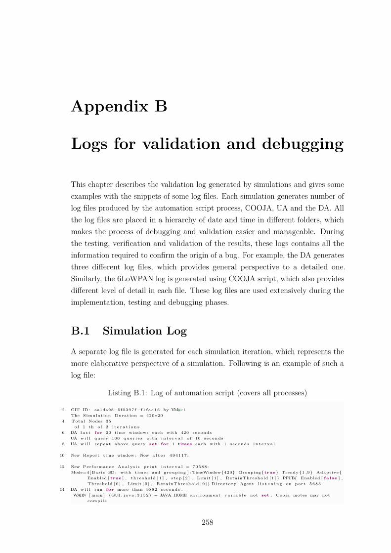
Appendix B
Logs for validation and debugging
This chapter describes the validation log generated by simulations and gives someexamples with the snippets of some log files. Each simulation generates number oflog files produced by the automation script process, COOJA, UA and the DA. Allthe log files are placed in a hierarchy of date and time in different folders, whichmakes the process of debugging and validation easier and manageable. Duringthe testing, verification and validation of the results, these logs contains all theinformation required to confirm the origin of a bug. For example, the DA generatesthree different log files, which provides general perspective to a detailed one.Similarly, the 6LoWPAN log is generated using COOJA script, which also providesdifferent level of detail in each file. These log files are used extensively during theimplementation, testing and debugging phases.
B.1 Simulation Log
A separate log file is generated for each simulation iteration, which represents themore elaborative perspective of a simulation. Following is an example of such alog file:
Listing B.1: Log of automation script (covers all processes)
2 GIT ID : aa1da98−5f 0 3 9 7 f −f 1 f a e 1 6 by VM#c1The S i mu la t io n Duration = 420∗20
4 Total Nodes 35o f 1 th o f 2 i t e r a t i o n s
6 DA l a s t for 20 time windows each with 420 secondsUA w i l l query 100 q u e r i e s with i n t e r v a l o f 10 seconds
8 UA w i l l r e p e a t above query set for 1 times each with 1 seconds i n t e r v a l
10 New Report time window : Now a f t e r 494117:
12 New Performance A n a l y s i s p r i n t i n t e r v a l = 7 0 5 8 8 :Mode=4[ Basic SD : with t imer and grouping ] : TimeWindow{420} Grouping {true} Trendy {1 ,9} Adaptive {
Enabled [ true ] , t h r e s h o l d [ 1 ] , s t e p [ 2 ] , Limit [ 1 ] , RetainThreshold [ 1 ] } PPUB{ Enabled [ f a l s e ] ,Threshold [ 0 ] , Limit [ 0 ] , RetainThreshold [ 0 ] } D i r e c t o r y Agent l i s t e n i n g on port 5 6 8 3 .
14 DA w i l l run for more than 9882 seconds .WARN [ main ] (GUI . java : 3 1 5 2 ) − JAVA_HOME environment v a r i a b l e not set , Cooja motes may not
compile
258
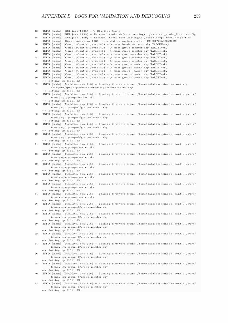
APPENDIX B. LOGS FOR VALIDATION AND DEBUGGING 259
16 INFO [ main ] (GUI . java : 1 3 2 5 ) − > S t a r t i n g CoojaINFO [ main ] (GUI . java : 2 8 3 9 ) − External t o o l s d e f a u l t s e t t i n g s : / e x t e r n a l _ t o o l s _ l i n u x . c o n f i g
18 INFO [ main ] (GUI . java : 2 8 6 9 ) − External t o o l s u s e r s e t t i n g s : / r o o t / . c o o j a . u s e r . p r o p e r t i e sINFO [ main ] ( S im ul a t i on . java : 4 2 3 ) − S im ul at i on random seed : −1948817365486295399
20 INFO [ main ] ( CompileContiki . java : 1 4 0 ) − > make border−r o u t e r . sky TARGET=skyINFO [ main ] ( CompileContiki . java : 1 4 0 ) − > make group−member . sky TARGET=sky
22 INFO [ main ] ( CompileContiki . java : 1 4 0 ) − > make group−member . sky TARGET=skyINFO [ main ] ( CompileContiki . java : 1 4 0 ) − > make group−member . sky TARGET=sky
24 INFO [ main ] ( CompileContiki . java : 1 4 0 ) − > make group−member . sky TARGET=skyINFO [ main ] ( CompileContiki . java : 1 4 0 ) − > make group−member . sky TARGET=sky
26 INFO [ main ] ( CompileContiki . java : 1 4 0 ) − > make group−l e a d e r . sky TARGET=skyINFO [ main ] ( CompileContiki . java : 1 4 0 ) − > make group−l e a d e r . sky TARGET=sky
28 INFO [ main ] ( CompileContiki . java : 1 4 0 ) − > make group−l e a d e r . sky TARGET=skyINFO [ main ] ( CompileContiki . java : 1 4 0 ) − > make group−l e a d e r . sky TARGET=sky
30 INFO [ main ] ( CompileContiki . java : 1 4 0 ) − > make group−l e a d e r . sky TARGET=sky∗∗∗ S e t t i n g up f1611 IO !
32 INFO [ main ] ( MspMote . java : 2 1 6 ) − Loading f irmware from : /home/ t a l a l / sen s inode −c o n t i k i /examples / ipv6 / rpl −border−r o u t e r / border−r o u t e r . sky
∗∗∗ S e t t i n g up f1611 IO !34 INFO [ main ] ( MspMote . java : 2 1 6 ) − Loading f irmware from : /home/ t a l a l / sen s inode −c o n t i k i /work/
trendy−g l / group−l e a d e r . sky∗∗∗ S e t t i n g up f1611 IO !
36 INFO [ main ] ( MspMote . java : 2 1 6 ) − Loading f irmware from : /home/ t a l a l / sen s inode −c o n t i k i /work/trendy−g l group −2/group−l e a d e r . sky
∗∗∗ S e t t i n g up f1611 IO !38 INFO [ main ] ( MspMote . java : 2 1 6 ) − Loading f irmware from : /home/ t a l a l / sen s inode −c o n t i k i /work/
trendy−g l group −3/group−l e a d e r . sky∗∗∗ S e t t i n g up f1611 IO !
40 INFO [ main ] ( MspMote . java : 2 1 6 ) − Loading f irmware from : /home/ t a l a l / sen s inode −c o n t i k i /work/trendy−g l group −4/group−l e a d e r . sky
∗∗∗ S e t t i n g up f1611 IO !42 INFO [ main ] ( MspMote . java : 2 1 6 ) − Loading f irmware from : /home/ t a l a l / sen s inode −c o n t i k i /work/
trendy−g l group −5/group−l e a d e r . sky∗∗∗ S e t t i n g up f1611 IO !
44 INFO [ main ] ( MspMote . java : 2 1 6 ) − Loading f irmware from : /home/ t a l a l / sen s inode −c o n t i k i /work/trendy−gm/ group−member . sky
∗∗∗ S e t t i n g up f1611 IO !46 INFO [ main ] ( MspMote . java : 2 1 6 ) − Loading f irmware from : /home/ t a l a l / sen s inode −c o n t i k i /work/
trendy−gm/ group−member . sky∗∗∗ S e t t i n g up f1611 IO !
48 INFO [ main ] ( MspMote . java : 2 1 6 ) − Loading f irmware from : /home/ t a l a l / sen s inode −c o n t i k i /work/trendy−gm/ group−member . sky
∗∗∗ S e t t i n g up f1611 IO !50 INFO [ main ] ( MspMote . java : 2 1 6 ) − Loading f irmware from : /home/ t a l a l / sen s inode −c o n t i k i /work/
trendy−gm/ group−member . sky∗∗∗ S e t t i n g up f1611 IO !
52 INFO [ main ] ( MspMote . java : 2 1 6 ) − Loading f irmware from : /home/ t a l a l / sen s inode −c o n t i k i /work/trendy−gm/ group−member . sky
∗∗∗ S e t t i n g up f1611 IO !54 INFO [ main ] ( MspMote . java : 2 1 6 ) − Loading f irmware from : /home/ t a l a l / sen s inode −c o n t i k i /work/
trendy−gm/ group−member . sky∗∗∗ S e t t i n g up f1611 IO !
56 INFO [ main ] ( MspMote . java : 2 1 6 ) − Loading f irmware from : /home/ t a l a l / sen s inode −c o n t i k i /work/trendy−gm group −2/group−member . sky
∗∗∗ S e t t i n g up f1611 IO !58 INFO [ main ] ( MspMote . java : 2 1 6 ) − Loading f irmware from : /home/ t a l a l / sen s inode −c o n t i k i /work/
trendy−gm group −2/group−member . sky∗∗∗ S e t t i n g up f1611 IO !
60 INFO [ main ] ( MspMote . java : 2 1 6 ) − Loading f irmware from : /home/ t a l a l / sen s inode −c o n t i k i /work/trendy−gm group −2/group−member . sky
∗∗∗ S e t t i n g up f1611 IO !62 INFO [ main ] ( MspMote . java : 2 1 6 ) − Loading f irmware from : /home/ t a l a l / sen s inode −c o n t i k i /work/
trendy−gm group −2/group−member . sky∗∗∗ S e t t i n g up f1611 IO !
64 INFO [ main ] ( MspMote . java : 2 1 6 ) − Loading f irmware from : /home/ t a l a l / sen s inode −c o n t i k i /work/trendy−gm group −2/group−member . sky
∗∗∗ S e t t i n g up f1611 IO !66 INFO [ main ] ( MspMote . java : 2 1 6 ) − Loading f irmware from : /home/ t a l a l / sen s inode −c o n t i k i /work/
trendy−gm group −2/group−member . sky∗∗∗ S e t t i n g up f1611 IO !
68 INFO [ main ] ( MspMote . java : 2 1 6 ) − Loading f irmware from : /home/ t a l a l / sen s inode −c o n t i k i /work/trendy−gm group −3/group−member . sky
∗∗∗ S e t t i n g up f1611 IO !70 INFO [ main ] ( MspMote . java : 2 1 6 ) − Loading f irmware from : /home/ t a l a l / sen s inode −c o n t i k i /work/
trendy−gm group −3/group−member . sky∗∗∗ S e t t i n g up f1611 IO !
72 INFO [ main ] ( MspMote . java : 2 1 6 ) − Loading f irmware from : /home/ t a l a l / sen s inode −c o n t i k i /work/trendy−gm group −3/group−member . sky
∗∗∗ S e t t i n g up f1611 IO !
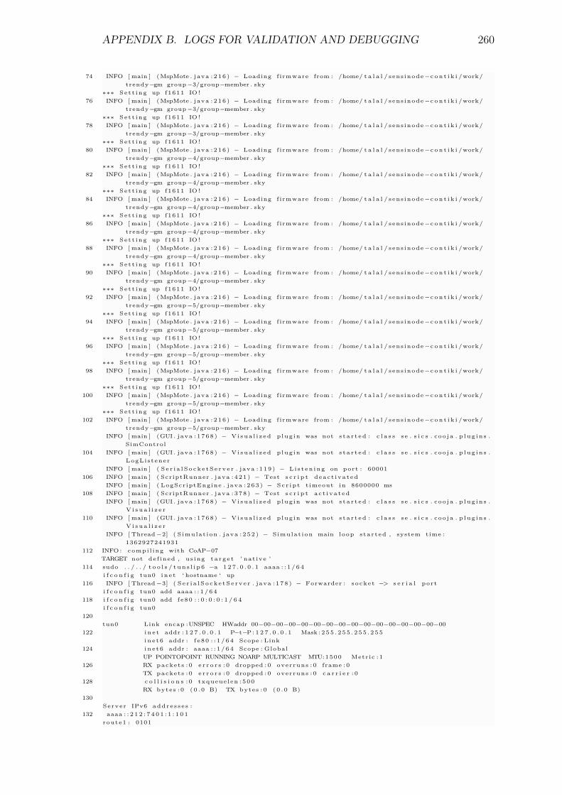
APPENDIX B. LOGS FOR VALIDATION AND DEBUGGING 260
74 INFO [ main ] ( MspMote . java : 2 1 6 ) − Loading f irmware from : /home/ t a l a l / sen s inode −c o n t i k i /work/trendy−gm group −3/group−member . sky
∗∗∗ S e t t i n g up f1611 IO !76 INFO [ main ] ( MspMote . java : 2 1 6 ) − Loading f irmware from : /home/ t a l a l / sen s inode −c o n t i k i /work/
trendy−gm group −3/group−member . sky∗∗∗ S e t t i n g up f1611 IO !
78 INFO [ main ] ( MspMote . java : 2 1 6 ) − Loading f irmware from : /home/ t a l a l / sen s inode −c o n t i k i /work/trendy−gm group −3/group−member . sky
∗∗∗ S e t t i n g up f1611 IO !80 INFO [ main ] ( MspMote . java : 2 1 6 ) − Loading f irmware from : /home/ t a l a l / sen s inode −c o n t i k i /work/
trendy−gm group −4/group−member . sky∗∗∗ S e t t i n g up f1611 IO !
82 INFO [ main ] ( MspMote . java : 2 1 6 ) − Loading f irmware from : /home/ t a l a l / sen s inode −c o n t i k i /work/trendy−gm group −4/group−member . sky
∗∗∗ S e t t i n g up f1611 IO !84 INFO [ main ] ( MspMote . java : 2 1 6 ) − Loading f irmware from : /home/ t a l a l / sen s inode −c o n t i k i /work/
trendy−gm group −4/group−member . sky∗∗∗ S e t t i n g up f1611 IO !
86 INFO [ main ] ( MspMote . java : 2 1 6 ) − Loading f irmware from : /home/ t a l a l / sen s inode −c o n t i k i /work/trendy−gm group −4/group−member . sky
∗∗∗ S e t t i n g up f1611 IO !88 INFO [ main ] ( MspMote . java : 2 1 6 ) − Loading f irmware from : /home/ t a l a l / sen s inode −c o n t i k i /work/
trendy−gm group −4/group−member . sky∗∗∗ S e t t i n g up f1611 IO !
90 INFO [ main ] ( MspMote . java : 2 1 6 ) − Loading f irmware from : /home/ t a l a l / sen s inode −c o n t i k i /work/trendy−gm group −4/group−member . sky
∗∗∗ S e t t i n g up f1611 IO !92 INFO [ main ] ( MspMote . java : 2 1 6 ) − Loading f irmware from : /home/ t a l a l / sen s inode −c o n t i k i /work/
trendy−gm group −5/group−member . sky∗∗∗ S e t t i n g up f1611 IO !
94 INFO [ main ] ( MspMote . java : 2 1 6 ) − Loading f irmware from : /home/ t a l a l / sen s inode −c o n t i k i /work/trendy−gm group −5/group−member . sky
∗∗∗ S e t t i n g up f1611 IO !96 INFO [ main ] ( MspMote . java : 2 1 6 ) − Loading f irmware from : /home/ t a l a l / sen s inode −c o n t i k i /work/
trendy−gm group −5/group−member . sky∗∗∗ S e t t i n g up f1611 IO !
98 INFO [ main ] ( MspMote . java : 2 1 6 ) − Loading f irmware from : /home/ t a l a l / sen s inode −c o n t i k i /work/trendy−gm group −5/group−member . sky
∗∗∗ S e t t i n g up f1611 IO !100 INFO [ main ] ( MspMote . java : 2 1 6 ) − Loading f irmware from : /home/ t a l a l / sen s inode −c o n t i k i /work/
trendy−gm group −5/group−member . sky∗∗∗ S e t t i n g up f1611 IO !
102 INFO [ main ] ( MspMote . java : 2 1 6 ) − Loading f irmware from : /home/ t a l a l / sen s inode −c o n t i k i /work/trendy−gm group −5/group−member . sky
INFO [ main ] (GUI . java : 1 7 6 8 ) − V i s u a l i z e d p l u g i n was not s t a r t e d : c l a s s s e . s i c s . c o o j a . p l u g i n s .SimControl
104 INFO [ main ] (GUI . java : 1 7 6 8 ) − V i s u a l i z e d p l u g i n was not s t a r t e d : c l a s s s e . s i c s . c o o j a . p l u g i n s .L o g L i s t e n e r
INFO [ main ] ( S e r i a l S o c k e t S e r v e r . java : 1 1 9 ) − L i s t e n i n g on port : 60001106 INFO [ main ] ( ScriptRunner . java : 4 2 1 ) − Test s c r i p t d e a c t i v a t e d
INFO [ main ] ( LogScriptEngine . java : 2 6 3 ) − S c r i p t timeout i n 8600000 ms108 INFO [ main ] ( ScriptRunner . java : 3 7 8 ) − Test s c r i p t a c t i v a t e d
INFO [ main ] (GUI . java : 1 7 6 8 ) − V i s u a l i z e d p l u g i n was not s t a r t e d : c l a s s s e . s i c s . c o o j a . p l u g i n s .V i s u a l i z e r
110 INFO [ main ] (GUI . java : 1 7 6 8 ) − V i s u a l i z e d p l u g i n was not s t a r t e d : c l a s s s e . s i c s . c o o j a . p l u g i n s .V i s u a l i z e r
INFO [ Thread −2] ( S i m ul at i on . java : 2 5 2 ) − S im ul a t i on main loop s t a r t e d , system time :1362927241931
112 INFO : c o m p i l i n g with CoAP−07TARGET not d e f i n e d , u s i n g t a r g e t ’ nat ive ’
114 sudo . . / . . / t o o l s / t u n s l i p 6 −a 1 2 7 . 0 . 0 . 1 aaaa : : 1 / 6 4i f c o n f i g tun0 i n e t ‘ hostname ‘ up
116 INFO [ Thread −3] ( S e r i a l S o c k e t S e r v e r . java : 1 7 8 ) − Forwarder : s o c k e t −> s e r i a l porti f c o n f i g tun0 add aaaa : : 1 / 6 4
118 i f c o n f i g tun0 add f e 8 0 : : 0 : 0 : 0 : 1 / 6 4i f c o n f i g tun0
120tun0 Link encap :UNSPEC HWaddr 00−00−00−00−00−00−00−00−00−00−00−00−00−00−00−00
122 i n e t addr : 1 2 7 . 0 . 0 . 1 P−t−P : 1 2 7 . 0 . 0 . 1 Mask : 2 5 5 . 2 5 5 . 2 5 5 . 2 5 5i n e t 6 addr : f e 8 0 : : 1 / 6 4 Scope : Link
124 i n e t 6 addr : aaaa : : 1 / 6 4 Scope : GlobalUP POINTOPOINT RUNNING NOARP MULTICAST MTU: 1 5 0 0 Metric : 1
126 RX p a c k e t s : 0 e r r o r s : 0 dropped : 0 o ver run s : 0 frame : 0TX p a c k e t s : 0 e r r o r s : 0 dropped : 0 o ver run s : 0 c a r r i e r : 0
128 c o l l i s i o n s : 0 t xq u eu el e n : 5 0 0RX bytes : 0 ( 0 . 0 B) TX bytes : 0 ( 0 . 0 B)
130S e r v e r IPv6 a d d r e s s e s :
132 aaaa : : 2 1 2 : 7 4 0 1 : 1 : 1 0 1r o u t e 1 : 0101
APPENDIX B. LOGS FOR VALIDATION AND DEBUGGING 261
134 f e 8 0 : : 2 1 2 : 7 4 0 1 : 1 : 1 0 1r o u t e 2 : 0101
136 S e r v e r IPv6 a d d r e s s e s :aaaa : : 2 1 2 : 7 4 0 1 : 1 : 1 0 1
138 r o u t e 1 : 0101f e 8 0 : : 2 1 2 : 7 4 0 1 : 1 : 1 0 1
140 r o u t e 2 : 0101event−r −1: 03−>03 −273
142 r −2: 05−>05 −273r −3: 0 f −>05 −265
144 r −4: 02−>02 −272r −5: 11−>02 −257
146 r −6: 0a−>05 −256r −7: 04−>04 −277
148 r −8: 1 f −>06 −271r −9: 0c−>02 −276
150 r −10: 08−>03 −267r −11: 06−>06 −276
152 r −12: 1a−>06 −256r −13: 18−>04 −267
154 r −14: 1e−>05 −264r −15: 15−>06 −270
156 r −16: 21−>03 −266r −17: 1c−>03 −267
158 r −18: 07−>02 −257r −19: 20−>02 −257
160 r −20: 13−>04 −267r −21: 19−>05 −267
162 r −22: 1b−>02 −256r −23: 17−>03 −265
164 r −24: 14−>05 −257r −25: 10−>06 −269
166 r −26: 0e−>04 −267r −27: 23−>05 −264
168 r −28: 0b−>06 −269r −29: 12−>03 −266
170 r −30: 09−>04 −267r −31: 24−>06 −270
172 r −32: 0d−>03 −268r −33: 22−>04 −265
174 r −34: 1d−>04 −266r −35: 16−>02 −264
176 Incoming r e q u e s t from / trendy / rep / trendy / repAdded Resource : URL[ trendy / g l ] ; [ , ] ; Cache [ for 0 minutes at 1362927409057]
178 ∗∗∗∗∗∗∗∗∗∗∗∗∗∗∗∗∗∗∗∗∗∗∗∗∗∗∗∗∗∗∗∗∗∗∗∗∗∗∗∗∗∗∗∗∗∗∗∗∗∗∗
180 A n a l y s i s o f R e g i s t r y for Grouping :
182 ∗∗∗∗∗∗∗∗∗∗∗∗∗∗∗∗∗∗∗∗∗∗∗∗∗∗∗∗∗∗∗∗∗∗∗∗∗∗∗∗∗∗∗∗∗∗∗∗∗∗∗New GL: so c h e c k i n g
184 Node Node{URI [ / trendy / rep ] , g l I P [ / aaaa : 0 : 0 : 0 : 2 1 2 : 7 4 0 5 : 5 : 5 0 5 ] Active [ true ( 1 ) ] trendy [ 1 / 1 ]GlChanged [ f a l s e ] l o c a t i o n [ jmf04 ] b a t t e r y L e v e l [ 0 ] currentNumberOfResources [ 1 ] Active S i n c e[ 1 3 6 2 9 2 7 4 0 9 0 4 5 ] }
186 ∗∗∗∗∗∗∗∗∗∗∗∗∗∗∗∗∗∗∗∗∗∗∗∗∗∗∗∗∗∗∗∗∗∗∗∗∗∗∗∗∗∗∗∗∗∗∗∗∗∗∗Incoming r e q u e s t from / trendy / rep / trendy / rep
188 Added Resource : URL[ trendy / g l ] ; [ , ] ; Cache [ for 0 minutes at 1362927412931]∗∗∗∗∗∗∗∗∗∗∗∗∗∗∗∗∗∗∗∗∗∗∗∗∗∗∗∗∗∗∗∗∗∗∗∗∗∗∗∗∗∗∗∗∗∗∗∗∗∗∗
190A n a l y s i s o f R e g i s t r y for Grouping :
192∗∗∗∗∗∗∗∗∗∗∗∗∗∗∗∗∗∗∗∗∗∗∗∗∗∗∗∗∗∗∗∗∗∗∗∗∗∗∗∗∗∗∗∗∗∗∗∗∗∗∗
194 New GL: so c h e c k i n gNode Node{URI [ / trendy / rep ] , g l I P [ / aaaa : 0 : 0 : 0 : 2 1 2 : 7 4 0 4 : 4 : 4 0 4 ] Active [ true ( 1 ) ] trendy [ 1 / 1 ]
GlChanged [ f a l s e ] l o c a t i o n [ rut03 ] b a t t e r y L e v e l [ 0 ] currentNumberOfResources [ 1 ] Active S i n c e[ 1 3 6 2 9 2 7 4 1 2 9 2 2 ] }
196∗∗∗∗∗∗∗∗∗∗∗∗∗∗∗∗∗∗∗∗∗∗∗∗∗∗∗∗∗∗∗∗∗∗∗∗∗∗∗∗∗∗∗∗∗∗∗∗∗∗∗
198 Incoming r e q u e s t from / trendy / rep / trendy / repAdded Resource : URL[ trendy / g l ] ; [ , ] ; Cache [ for 0 minutes at 1362927417711]
200 ∗∗∗∗∗∗∗∗∗∗∗∗∗∗∗∗∗∗∗∗∗∗∗∗∗∗∗∗∗∗∗∗∗∗∗∗∗∗∗∗∗∗∗∗∗∗∗∗∗∗∗
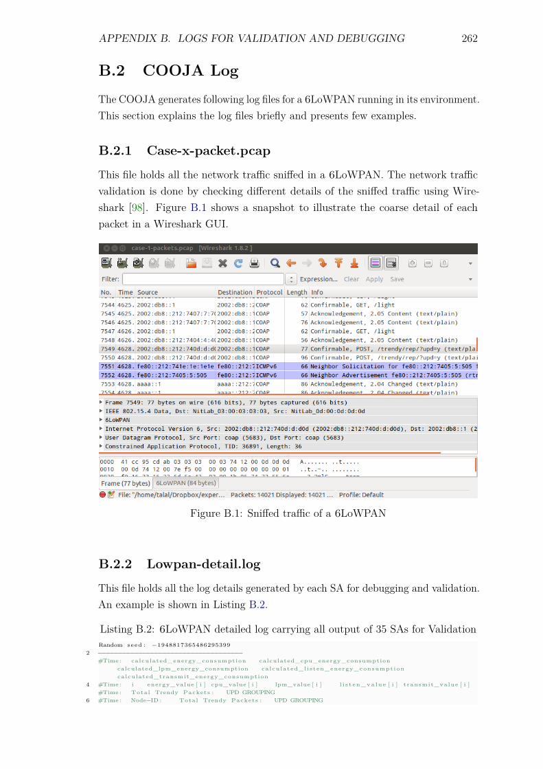
APPENDIX B. LOGS FOR VALIDATION AND DEBUGGING 262
B.2 COOJA Log
The COOJA generates following log files for a 6LoWPAN running in its environment.This section explains the log files briefly and presents few examples.
B.2.1 Case-x-packet.pcap
This file holds all the network traffic sniffed in a 6LoWPAN. The network trafficvalidation is done by checking different details of the sniffed traffic using Wire-shark [98]. Figure B.1 shows a snapshot to illustrate the coarse detail of eachpacket in a Wireshark GUI.
Figure B.1: Sniffed traffic of a 6LoWPAN
B.2.2 Lowpan-detail.log
This file holds all the log details generated by each SA for debugging and validation.An example is shown in Listing B.2.
Listing B.2: 6LoWPAN detailed log carrying all output of 35 SAs for ValidationRandom seed : −1948817365486295399
2 −−−−−−−−−−−−−−−−−−−−−−−−−−−−−−−−−−−−#Time : calculated_energy_consumption calculated_cpu_energy_consumption
calculated_lpm_energy_consumption calculated_l isten_energy_consumptioncalculated_transmit_energy_consumption
4 #Time : i energy_value [ i ] cpu_value [ i ] lpm_value [ i ] l i s t e n _ v a l u e [ i ] transmit_value [ i ]#Time : Total Trendy Packets : UPD GROUPING
6 #Time : Node−ID : Total Trendy Packets : UPD GROUPING
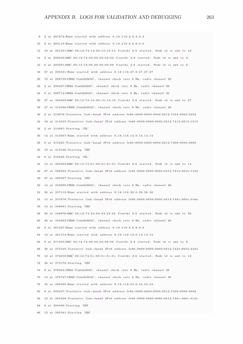
APPENDIX B. LOGS FOR VALIDATION AND DEBUGGING 263
8 2 at 281872: Rime s t a r t e d with a d d r e s s 0 . 1 8 . 1 1 6 . 2 . 0 . 2 . 2 . 2
10 6 at 283119: Rime s t a r t e d with a d d r e s s 0 . 1 8 . 1 1 6 . 6 . 0 . 6 . 6 . 6
12 19 at 291251:MAC 0 0 : 1 2 : 7 4 : 1 3 : 0 0 : 1 3 : 1 3 : 1 3 C o n t i k i 2 . 6 s t a r t e d . Node i d i s set to 1 9 .
14 2 at 292046:MAC 0 0 : 1 2 : 7 4 : 0 2 : 0 0 : 0 2 : 0 2 : 0 2 C o n t i k i 2 . 6 s t a r t e d . Node i d i s set to 2 .
16 6 at 293291:MAC 0 0 : 1 2 : 7 4 : 0 6 : 0 0 : 0 6 : 0 6 : 0 6 C o n t i k i 2 . 6 s t a r t e d . Node i d i s set to 6 .
18 27 at 293331: Rime s t a r t e d with a d d r e s s 0 . 1 8 . 1 1 6 . 2 7 . 0 . 2 7 . 2 7 . 2 7
20 19 at 298739:CSMA ContikiMAC , channel check r a t e 8 Hz , r a d i o channel 26
22 2 at 299467:CSMA ContikiMAC , channel check r a t e 8 Hz , r a d i o channel 26
24 6 at 300714:CSMA ContikiMAC , channel check r a t e 8 Hz , r a d i o channel 26
26 27 at 305099:MAC 0 0 : 1 2 : 7 4 : 1 b : 0 0 : 1 b : 1 b : 1 b C o n t i k i 2 . 6 s t a r t e d . Node i d i s set to 2 7 .
28 27 at 312586:CSMA ContikiMAC , channel check r a t e 8 Hz , r a d i o channel 26
30 2 at 313978: Tentat ive l i n k −l o c a l IPv6 a d d r e s s f e 8 0 : 0 0 0 0 : 0 0 0 0 : 0 0 0 0 : 0 2 1 2 : 7 4 0 2 : 0 0 0 2 : 0 2 0 2
32 19 at 314543: Tentat ive l i n k −l o c a l IPv6 a d d r e s s f e 8 0 : 0 0 0 0 : 0 0 0 0 : 0 0 0 0 : 0 2 1 2 : 7 4 1 3 : 0 0 1 3 : 1 3 1 3
34 2 at 314981: S t a r t i n g ’GL’
36 14 at 315067: Rime s t a r t e d with a d d r e s s 0 . 1 8 . 1 1 6 . 1 4 . 0 . 1 4 . 1 4 . 1 4
38 6 at 315225: Tentat ive l i n k −l o c a l IPv6 a d d r e s s f e 8 0 : 0 0 0 0 : 0 0 0 0 : 0 0 0 0 : 0 2 1 2 : 7 4 0 6 : 0 0 0 6 : 0 6 0 6
40 19 at 315546: S t a r t i n g ’GM’
42 6 at 316228: S t a r t i n g ’GL’
44 14 at 325603:MAC 0 0 : 1 2 : 7 4 : 0 e : 0 0 : 0 e : 0 e : 0 e C o n t i k i 2 . 6 s t a r t e d . Node i d i s set to 1 4 .
46 27 at 328394: Tentat ive l i n k −l o c a l IPv6 a d d r e s s f e 8 0 : 0 0 0 0 : 0 0 0 0 : 0 0 0 0 : 0 2 1 2 : 7 4 1 b : 0 0 1 b : 1 b1b
48 27 at 329397: S t a r t i n g ’GM’
50 14 at 333090:CSMA ContikiMAC , channel check r a t e 8 Hz , r a d i o channel 26
52 36 at 337112: Rime s t a r t e d with a d d r e s s 0 . 1 8 . 1 1 6 . 3 6 . 0 . 3 6 . 3 6 . 3 6
54 14 at 347678: Tentat ive l i n k −l o c a l IPv6 a d d r e s s f e 8 0 : 0 0 0 0 : 0 0 0 0 : 0 0 0 0 : 0 2 1 2 : 7 4 0 e : 0 0 0 e : 0 e0e
56 14 at 348681: S t a r t i n g ’GM’
58 36 at 348876:MAC 0 0 : 1 2 : 7 4 : 2 4 : 0 0 : 2 4 : 2 4 : 2 4 C o n t i k i 2 . 6 s t a r t e d . Node i d i s set to 3 6 .
60 36 at 356363:CSMA ContikiMAC , channel check r a t e 8 Hz , r a d i o channel 26
62 8 at 361327: Rime s t a r t e d with a d d r e s s 0 . 1 8 . 1 1 6 . 8 . 0 . 8 . 8 . 8
64 12 at 361714: Rime s t a r t e d with a d d r e s s 0 . 1 8 . 1 1 6 . 1 2 . 0 . 1 2 . 1 2 . 1 2
66 8 at 371503:MAC 0 0 : 1 2 : 7 4 : 0 8 : 0 0 : 0 8 : 0 8 : 0 8 C o n t i k i 2 . 6 s t a r t e d . Node i d i s set to 8 .
68 36 at 372165: Tentat ive l i n k −l o c a l IPv6 a d d r e s s f e 8 0 : 0 0 0 0 : 0 0 0 0 : 0 0 0 0 : 0 2 1 2 : 7 4 2 4 : 0 0 2 4 : 2 4 2 4
70 12 at 372259:MAC 0 0 : 1 2 : 7 4 : 0 c : 0 0 : 0 c : 0 c : 0 c C o n t i k i 2 . 6 s t a r t e d . Node i d i s set to 1 2 .
72 36 at 373172: S t a r t i n g ’GM’
74 8 at 378924:CSMA ContikiMAC , channel check r a t e 8 Hz , r a d i o channel 26
76 12 at 379747:CSMA ContikiMAC , channel check r a t e 8 Hz , r a d i o channel 26
78 34 at 390495: Rime s t a r t e d with a d d r e s s 0 . 1 8 . 1 1 6 . 3 4 . 0 . 3 4 . 3 4 . 3 4
80 8 at 393437: Tentat ive l i n k −l o c a l IPv6 a d d r e s s f e 8 0 : 0 0 0 0 : 0 0 0 0 : 0 0 0 0 : 0 2 1 2 : 7 4 0 8 : 0 0 0 8 : 0 8 0 8
82 12 at 394338: Tentat ive l i n k −l o c a l IPv6 a d d r e s s f e 8 0 : 0 0 0 0 : 0 0 0 0 : 0 0 0 0 : 0 2 1 2 : 7 4 0 c : 0 0 0 c : 0 c0c
84 8 at 394440: S t a r t i n g ’GM’
86 12 at 395341: S t a r t i n g ’GM’
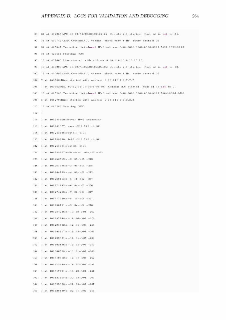
APPENDIX B. LOGS FOR VALIDATION AND DEBUGGING 264
88 34 at 402255:MAC 0 0 : 1 2 : 7 4 : 2 2 : 0 0 : 2 2 : 2 2 : 2 2 C o n t i k i 2 . 6 s t a r t e d . Node i d i s set to 3 4 .
90 34 at 409742:CSMA ContikiMAC , channel check r a t e 8 Hz , r a d i o channel 26
92 34 at 425547: Tentat ive l i n k −l o c a l IPv6 a d d r e s s f e 8 0 : 0 0 0 0 : 0 0 0 0 : 0 0 0 0 : 0 2 1 2 : 7 4 2 2 : 0 0 2 2 : 2 2 2 2
94 34 at 426551: S t a r t i n g ’GM’
96 13 at 432660: Rime s t a r t e d with a d d r e s s 0 . 1 8 . 1 1 6 . 1 3 . 0 . 1 3 . 1 3 . 1 3
98 13 at 443208:MAC 0 0 : 1 2 : 7 4 : 0 d : 0 0 : 0 d : 0 d : 0 d C o n t i k i 2 . 6 s t a r t e d . Node i d i s set to 1 3 .
100 13 at 450695:CSMA ContikiMAC , channel check r a t e 8 Hz , r a d i o channel 26
102 7 at 453583: Rime s t a r t e d with a d d r e s s 0 . 1 8 . 1 1 6 . 7 . 0 . 7 . 7 . 7
104 7 at 463762:MAC 0 0 : 1 2 : 7 4 : 0 7 : 0 0 : 0 7 : 0 7 : 0 7 C o n t i k i 2 . 6 s t a r t e d . Node i d i s set to 7 .
106 13 at 465283: Tentat ive l i n k −l o c a l IPv6 a d d r e s s f e 8 0 : 0 0 0 0 : 0 0 0 0 : 0 0 0 0 : 0 2 1 2 : 7 4 0 d : 0 0 0 d : 0 d0d
108 3 at 466279: Rime s t a r t e d with a d d r e s s 0 . 1 8 . 1 1 6 . 3 . 0 . 3 . 3 . 3
110 13 at 466286: S t a r t i n g ’GM’.
112 ..
114 1 at 109235400: S e r v e r IPv6 a d d r e s s e s :
116 1 at 109241677: aaaa : : 2 1 2 : 7 4 0 1 : 1 : 1 0 1
118 1 at 109243638: r o u t e 1 : 0101
120 1 at 109249930: f e 8 0 : : 2 1 2 : 7 4 0 1 : 1 : 1 0 1
122 1 at 109251891: r o u t e 2 : 0101
124 1 at 109255367: event−r −1: 03−>03 −273
126 1 at 109258519: r −2: 05−>05 −273
128 1 at 109261588: r −3: 0 f −>05 −265
130 1 at 109264739: r −4: 02−>02 −272
132 1 at 109268113: r −5: 11−>02 −257
134 1 at 109271183: r −6: 0a−>05 −256
136 1 at 109274263: r −7: 04−>04 −277
138 1 at 109277639: r −8: 1 f −>06 −271
140 1 at 109280791: r −9: 0c−>02 −276
142 1 at 109284228: r −10: 08−>03 −267
144 1 at 109287748: r −11: 06−>06 −276
146 1 at 109291492: r −12: 1a−>06 −256
148 1 at 109295317: r −13: 18−>04 −267
150 1 at 109299061: r −14: 1e−>05 −264
152 1 at 109302826: r −15: 15−>06 −270
154 1 at 109306568: r −16: 21−>03 −266
156 1 at 109310312: r −17: 1c−>03 −267
158 1 at 109313749: r −18: 07−>02 −257
160 1 at 109317491: r −19: 20−>02 −257
162 1 at 109321315: r −20: 13−>04 −267
164 1 at 109325058: r −21: 19−>05 −267
166 1 at 109328839: r −22: 1b−>02 −256
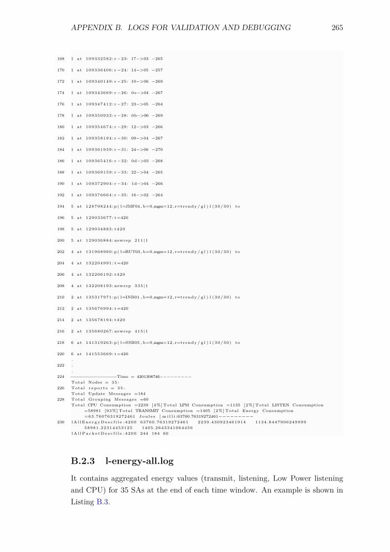
APPENDIX B. LOGS FOR VALIDATION AND DEBUGGING 265
168 1 at 109332582: r −23: 17−>03 −265
170 1 at 109336406: r −24: 14−>05 −257
172 1 at 109340149: r −25: 10−>06 −269
174 1 at 109343669: r −26: 0e−>04 −267
176 1 at 109347412: r −27: 23−>05 −264
178 1 at 109350932: r −28: 0b−>06 −269
180 1 at 109354674: r −29: 12−>03 −266
182 1 at 109358194: r −30: 09−>04 −267
184 1 at 109361939: r −31: 24−>06 −270
186 1 at 109365416: r −32: 0d−>03 −268
188 1 at 109369159: r −33: 22−>04 −265
190 1 at 109372904: r −34: 1d−>04 −266
192 1 at 109376664: r −35: 16−>02 −264
194 5 at 128798244: p ( l=JMF04 , b=0,mgm=12 , r=trendy / g l ) l (30/30) to
196 5 at 129033677: t =420
198 5 at 129034883: t420
200 5 at 129036884: newrep 21 1| 1
202 4 at 131968960: p ( l=RUT03, b=0,mgm=12 , r=trendy / g l ) l (30/30) to
204 4 at 132204991: t =420
206 4 at 132206192: t420
208 4 at 132208193: newrep 33 5| 1
210 2 at 135317971: p ( l=INB01 , b=0,mgm=12 , r=trendy / g l ) l (30/30) to
212 2 at 135676994: t =420
214 2 at 135678194: t420
216 2 at 135680267: newrep 41 5| 1
218 6 at 141319263: p ( l=SSB05 , b=0,mgm=12 , r=trendy / g l ) l (30/30) to
220 6 at 141553669: t =420.
222 ..
224 −−−−−−−−−−−−−−−−Time = 4201308746−−−−−−−−−Total Nodes = 3 5 :
226 Total r e p o r t s = 3 5 :Total Update Messages =184
228 Total Grouping Messages =60Total CPU Consumption =2239 [4%] Total LPM Consumption =1135 [2%] Total LISTEN Consumption
=58981 [93%] Total TRANSMIT Consumption =1405 [2%] Total Energy Consumption=63.76076319272461 J o u l e s [ m i l l i :63760.76319272461−−−−−−−−−
230 l A l l E n e r g y D e s c f i l e : 4 2 0 0 63760.76319272461 2239.430923461914 1134.844790624999958981.22314453125 1405.2643341064456
l A l l P a c k e t D e s c f i l e : 4 2 0 0 244 184 60
B.2.3 l-energy-all.log
It contains aggregated energy values (transmit, listening, Low Power listeningand CPU) for 35 SAs at the end of each time window. An example is shown inListing B.3.
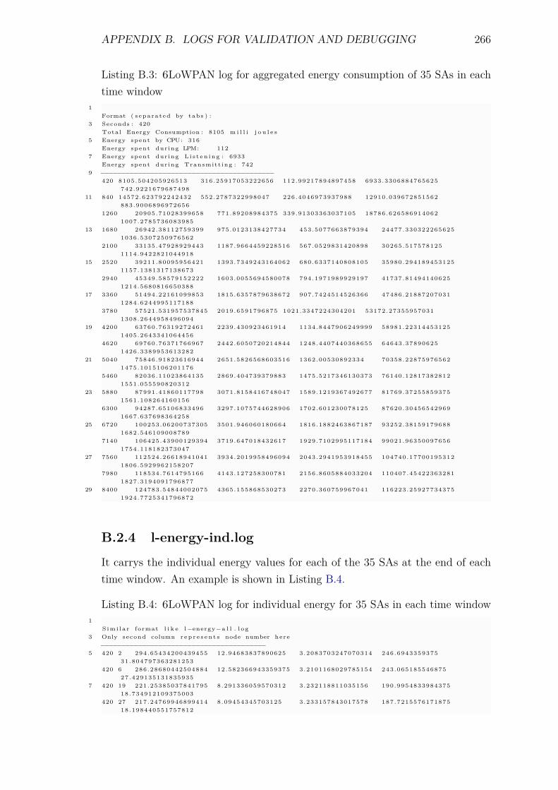
APPENDIX B. LOGS FOR VALIDATION AND DEBUGGING 266
Listing B.3: 6LoWPAN log for aggregated energy consumption of 35 SAs in eachtime window
1Format ( s e p a r a t e d by tabs ) :
3 Seconds : 420Total Energy Consumption : 8105 m i l l i j o u l e s
5 Energy spent by CPU: 316Energy spent during LPM: 112
7 Energy spent during L i s t e n i n g : 6933Energy spent during Transmitt ing : 742
9 −−−−−−−−−−−−−−−−−−−−−−−−−−−−−−−−−−−−−−−−−−420 8105.504205926513 316.25917053222656 112.99217894897458 6933.3306884765625
742.922167968749811 840 14572.623792242432 552.2787322998047 226.4046973937988 12910.039672851562
883.90068969726561260 20905.71028399658 771.89208984375 339.91303363037105 18786.626586914062
1007.278573608398513 1680 26942.38112759399 975.0123138427734 453.5077663879394 24477.330322265625
1036.53072509765622100 33135.47928929443 1187.9664459228516 567.0529831420898 30265.517578125
1114.942282104491815 2520 39211.80095956421 1393.7349243164062 680.6337140808105 35980.294189453125
1157.13813171386732940 45349.58579152222 1603.0055694580078 794.1971989929197 41737.81494140625
1214.568081665038817 3360 51494.22161099853 1815.6357879638672 907.7424514526366 47486.21887207031
1284.62449951171883780 57521.531957537845 2019.6591796875 1021.3347224304201 53172.27355957031
1308.264495849609419 4200 63760.76319272461 2239.430923461914 1134.8447906249999 58981.22314453125
1405.26433410644564620 69760.76371766967 2442.6050720214844 1248.4407440368655 64643.37890625
1426.338995361328221 5040 75846.91823616944 2651.5826568603516 1362.00530892334 70358.22875976562
1475.10151062011765460 82036.11023864135 2869.404739379883 1475.5217346130373 76140.12817382812
1551.05559082031223 5880 87991.41860117798 3071.8158416748047 1589.1219367492677 81769.37255859375
1561.1082641601566300 94287.65106833496 3297.1075744628906 1702.601230078125 87620.30456542969
1667.63769836425825 6720 100253.06200737305 3501.946060180664 1816.1882463867187 93252.38159179688
1682.5461090087897140 106425.43900129394 3719.647018432617 1929.7102995117184 99021.96350097656
1754.11818237304727 7560 112524.26618941041 3934.2019958496094 2043.2941953918455 104740.17700195312
1806.59299621582077980 118534.7614795166 4143.127258300781 2156.8605884033204 110407.45422363281
1827.319409179687729 8400 124783.54844002075 4365.155868530273 2270.360759967041 116223.25927734375
1924.7725341796872
B.2.4 l-energy-ind.log
It carrys the individual energy values for each of the 35 SAs at the end of eachtime window. An example is shown in Listing B.4.
Listing B.4: 6LoWPAN log for individual energy for 35 SAs in each time window1
S i m i l a r format l i k e l−energy−a l l . l o g3 Only second column r e p r e s e n t s node number here
−−−−−−−−−−−−−−−−−−−−−−−−−−−−−−−−−−−−−−−−5 420 2 294.65434200439455 12.94683837890625 3.2083703247070314 246.6943359375
31.804797363281253420 6 286.28680442504884 12.582366943359375 3.2101168029785154 243.065185546875
27.4291351318359357 420 19 221.25385037841795 8.291336059570312 3.232118811035156 190.9954833984375
18.734912109375003420 27 217.24769946899414 8.09454345703125 3.233157843017578 187.7215576171875
18.198440551757812
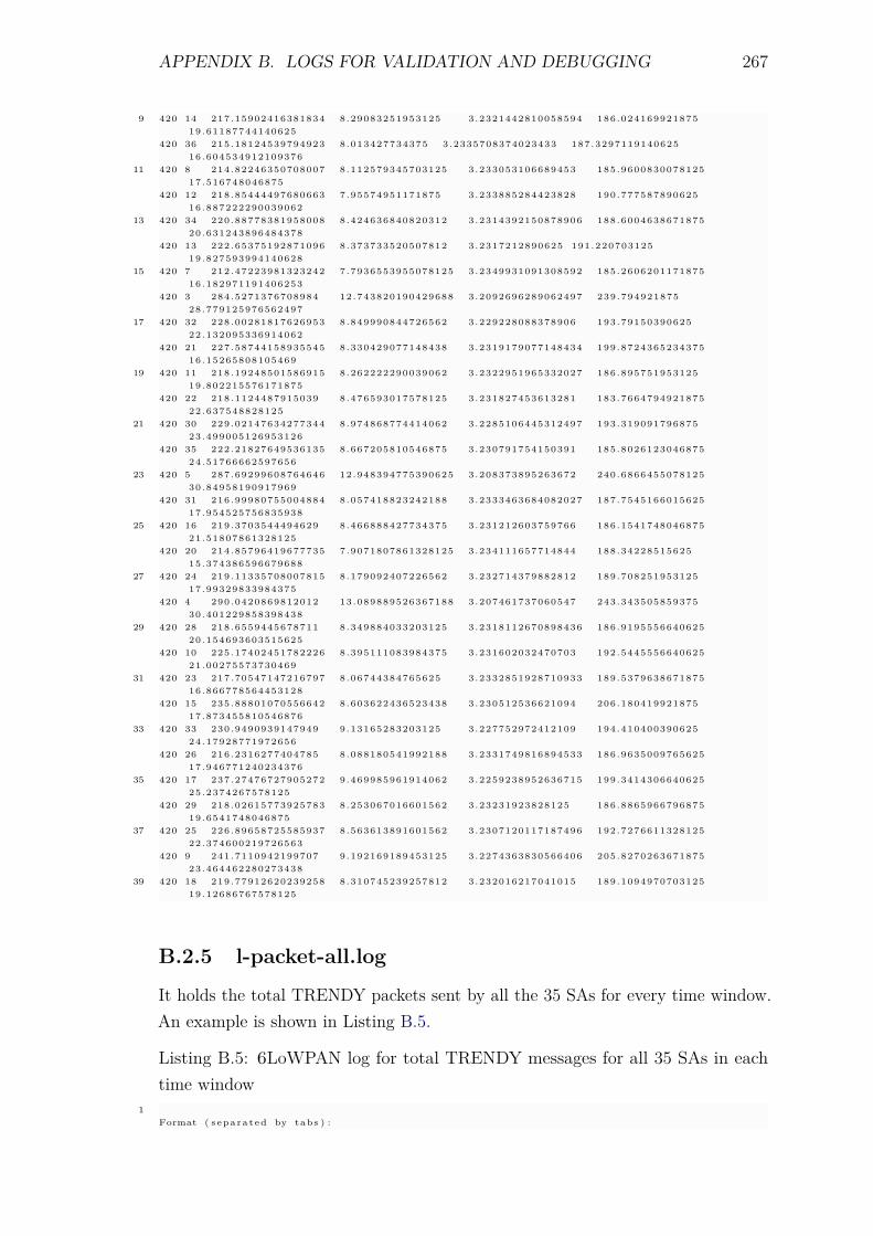
APPENDIX B. LOGS FOR VALIDATION AND DEBUGGING 267
9 420 14 217.15902416381834 8.29083251953125 3.2321442810058594 186.02416992187519.61187744140625
420 36 215.18124539794923 8.013427734375 3.2335708374023433 187.329711914062516.604534912109376
11 420 8 214.82246350708007 8.112579345703125 3.233053106689453 185.960083007812517.516748046875
420 12 218.85444497680663 7.95574951171875 3.233885284423828 190.77758789062516.887222290039062
13 420 34 220.88778381958008 8.424636840820312 3.2314392150878906 188.600463867187520.631243896484378
420 13 222.65375192871096 8.373733520507812 3.2317212890625 191.22070312519.827593994140628
15 420 7 212.47223981323242 7.7936553955078125 3.2349931091308592 185.260620117187516.182971191406253
420 3 284.5271376708984 12.743820190429688 3.2092696289062497 239.79492187528.779125976562497
17 420 32 228.00281817626953 8.849990844726562 3.229228088378906 193.7915039062522.132095336914062
420 21 227.58744158935545 8.330429077148438 3.2319179077148434 199.872436523437516.15265808105469
19 420 11 218.19248501586915 8.262222290039062 3.2322951965332027 186.89575195312519.802215576171875
420 22 218.1124487915039 8.476593017578125 3.231827453613281 183.766479492187522.637548828125
21 420 30 229.02147634277344 8.974868774414062 3.2285106445312497 193.31909179687523.499005126953126
420 35 222.21827649536135 8.667205810546875 3.230791754150391 185.802612304687524.51766662597656
23 420 5 287.69299608764646 12.948394775390625 3.208373895263672 240.686645507812530.84958190917969
420 31 216.99980755004884 8.057418823242188 3.2333463684082027 187.754516601562517.954525756835938
25 420 16 219.3703544494629 8.466888427734375 3.231212603759766 186.154174804687521.51807861328125
420 20 214.85796419677735 7.9071807861328125 3.234111657714844 188.3422851562515.374386596679688
27 420 24 219.11335708007815 8.179092407226562 3.232714379882812 189.70825195312517.99329833984375
420 4 290.0420869812012 13.089889526367188 3.207461737060547 243.34350585937530.401229858398438
29 420 28 218.6559445678711 8.349884033203125 3.2318112670898436 186.919555664062520.154693603515625
420 10 225.17402451782226 8.395111083984375 3.231602032470703 192.544555664062521.00275573730469
31 420 23 217.70547147216797 8.06744384765625 3.2332851928710933 189.537963867187516.866778564453128
420 15 235.88801070556642 8.603622436523438 3.230512536621094 206.18041992187517.873455810546876
33 420 33 230.9490939147949 9.13165283203125 3.227752972412109 194.41040039062524.17928771972656
420 26 216.2316277404785 8.088180541992188 3.2331749816894533 186.963500976562517.946771240234376
35 420 17 237.27476727905272 9.469985961914062 3.2259238952636715 199.341430664062525.2374267578125
420 29 218.02615773925783 8.253067016601562 3.23231923828125 186.886596679687519.6541748046875
37 420 25 226.89658725585937 8.563613891601562 3.2307120117187496 192.727661132812522.374600219726563
420 9 241.7110942199707 9.192169189453125 3.2274363830566406 205.827026367187523.464462280273438
39 420 18 219.77912620239258 8.310745239257812 3.232016217041015 189.109497070312519.12686767578125
B.2.5 l-packet-all.log
It holds the total TRENDY packets sent by all the 35 SAs for every time window.An example is shown in Listing B.5.
Listing B.5: 6LoWPAN log for total TRENDY messages for all 35 SAs in eachtime window
1Format ( s e p a r a t e d by tabs ) :
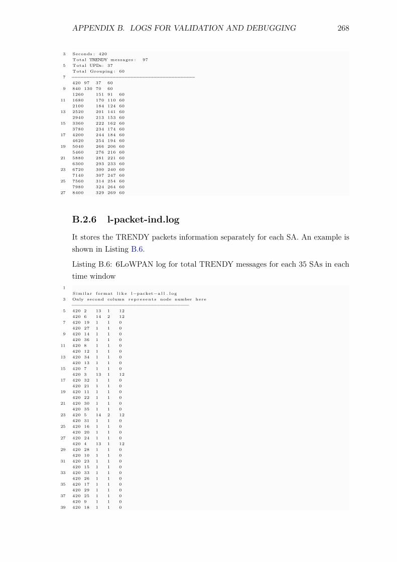
APPENDIX B. LOGS FOR VALIDATION AND DEBUGGING 268
3 Seconds : 420Total TRENDY messages : 97
5 Total UPDs : 37Total Grouping : 60
7 −−−−−−−−−−−−−−−−−−−−−−−−−−−−−−−−−−−−−−−−−−420 97 37 60
9 840 130 70 601260 151 91 60
11 1680 170 110 602100 184 124 60
13 2520 201 141 602940 213 153 60
15 3360 222 162 603780 234 174 60
17 4200 244 184 604620 254 194 60
19 5040 266 206 605460 276 216 60
21 5880 281 221 606300 293 233 60
23 6720 300 240 607140 307 247 60
25 7560 314 254 607980 324 264 60
27 8400 329 269 60
B.2.6 l-packet-ind.log
It stores the TRENDY packets information separately for each SA. An example isshown in Listing B.6.
Listing B.6: 6LoWPAN log for total TRENDY messages for each 35 SAs in eachtime window
1S i m i l a r format l i k e l−packet−a l l . l o g
3 Only second column r e p r e s e n t s node number here−−−−−−−−−−−−−−−−−−−−−−−−−−−−−−−−−−−−−−−−
5 420 2 13 1 12420 6 14 2 12
7 420 19 1 1 0420 27 1 1 0
9 420 14 1 1 0420 36 1 1 0
11 420 8 1 1 0420 12 1 1 0
13 420 34 1 1 0420 13 1 1 0
15 420 7 1 1 0420 3 13 1 12
17 420 32 1 1 0420 21 1 1 0
19 420 11 1 1 0420 22 1 1 0
21 420 30 1 1 0420 35 1 1 0
23 420 5 14 2 12420 31 1 1 0
25 420 16 1 1 0420 20 1 1 0
27 420 24 1 1 0420 4 13 1 12
29 420 28 1 1 0420 10 1 1 0
31 420 23 1 1 0420 15 1 1 0
33 420 33 1 1 0420 26 1 1 0
35 420 17 1 1 0420 29 1 1 0
37 420 25 1 1 0420 9 1 1 0
39 420 18 1 1 0
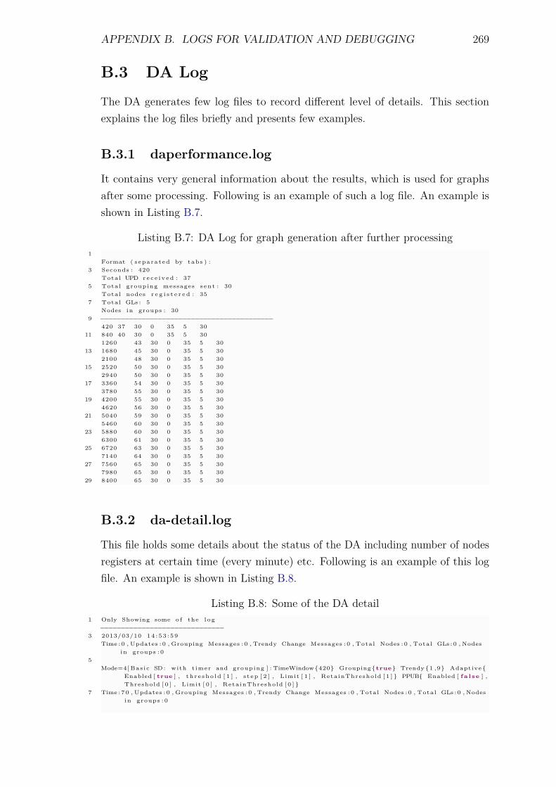
APPENDIX B. LOGS FOR VALIDATION AND DEBUGGING 269
B.3 DA Log
The DA generates few log files to record different level of details. This sectionexplains the log files briefly and presents few examples.
B.3.1 daperformance.log
It contains very general information about the results, which is used for graphsafter some processing. Following is an example of such a log file. An example isshown in Listing B.7.
Listing B.7: DA Log for graph generation after further processing1
Format ( s e p a r a t e d by tabs ) :3 Seconds : 420
Total UPD r e c e i v e d : 375 Total grouping messages s e n t : 30
Total nodes r e g i s t e r e d : 357 Total GLs : 5
Nodes i n groups : 309 −−−−−−−−−−−−−−−−−−−−−−−−−−−−−−−−−−−−−−−−−−
420 37 30 0 35 5 3011 840 40 30 0 35 5 30
1260 43 30 0 35 5 3013 1680 45 30 0 35 5 30
2100 48 30 0 35 5 3015 2520 50 30 0 35 5 30
2940 50 30 0 35 5 3017 3360 54 30 0 35 5 30
3780 55 30 0 35 5 3019 4200 55 30 0 35 5 30
4620 56 30 0 35 5 3021 5040 59 30 0 35 5 30
5460 60 30 0 35 5 3023 5880 60 30 0 35 5 30
6300 61 30 0 35 5 3025 6720 63 30 0 35 5 30
7140 64 30 0 35 5 3027 7560 65 30 0 35 5 30
7980 65 30 0 35 5 3029 8400 65 30 0 35 5 30
B.3.2 da-detail.log
This file holds some details about the status of the DA including number of nodesregisters at certain time (every minute) etc. Following is an example of this logfile. An example is shown in Listing B.8.
Listing B.8: Some of the DA detail1 Only Showing some o f the l o g
−−−−−−−−−−−−−−−−−−−−−−−−−−−−−−3 2013/03/10 1 4 : 5 3 : 5 9
Time : 0 , Updates : 0 , Grouping Messages : 0 , Trendy Change Messages : 0 , Total Nodes : 0 , Total GLs : 0 , Nodesi n groups : 0
5Mode=4[ Basic SD : with t imer and grouping ] : TimeWindow{420} Grouping {true} Trendy {1 ,9} Adaptive {
Enabled [ true ] , t h r e s h o l d [ 1 ] , s t e p [ 2 ] , Limit [ 1 ] , RetainThreshold [ 1 ] } PPUB{ Enabled [ f a l s e ] ,Threshold [ 0 ] , Limit [ 0 ] , RetainThreshold [ 0 ] }
7 Time : 7 0 , Updates : 0 , Grouping Messages : 0 , Trendy Change Messages : 0 , Total Nodes : 0 , Total GLs : 0 , Nodesi n groups : 0
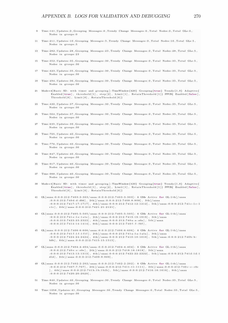
APPENDIX B. LOGS FOR VALIDATION AND DEBUGGING 270
9 Time : 1 4 1 , Updates : 0 , Grouping Messages : 0 , Trendy Change Messages : 0 , Total Nodes : 0 , Total GLs : 0 ,Nodes i n groups : 0
11 Time : 2 1 1 , Updates : 1 0 , Grouping Messages : 5 , Trendy Change Messages : 0 , Total Nodes : 1 0 , Total GLs : 5 ,Nodes i n groups : 5
13 Time : 2 8 2 , Updates : 2 8 , Grouping Messages : 2 3 , Trendy Change Messages : 0 , Total Nodes : 2 8 , Total GLs : 5 ,Nodes i n groups : 2 3
15 Time : 3 5 2 , Updates : 3 5 , Grouping Messages : 3 0 , Trendy Change Messages : 0 , Total Nodes : 3 5 , Total GLs : 5 ,Nodes i n groups : 3 0
17 Time : 4 2 3 , Updates : 3 5 , Grouping Messages : 3 0 , Trendy Change Messages : 0 , Total Nodes : 3 5 , Total GLs : 5 ,Nodes i n groups : 3 0
19 Time : 4 9 4 , Updates : 3 6 , Grouping Messages : 3 0 , Trendy Change Messages : 0 , Total Nodes : 3 5 , Total GLs : 5 ,Nodes i n groups : 3 0
21 Mode=4[ Basic SD : with t imer and grouping ] : TimeWindow{420} Grouping {true} Trendy {1 ,9} Adaptive {Enabled [ true ] , t h r e s h o l d [ 1 ] , s t e p [ 2 ] , Limit [ 1 ] , RetainThreshold [ 1 ] } PPUB{ Enabled [ f a l s e ] ,Threshold [ 0 ] , Limit [ 0 ] , RetainThreshold [ 0 ] }
23 Time : 4 2 0 , Updates : 3 7 , Grouping Messages : 3 0 , Trendy Change Messages : 0 , Total Nodes : 3 5 , Total GLs : 5 ,Nodes i n groups : 3 0
25 Time : 5 6 4 , Updates : 3 7 , Grouping Messages : 3 0 , Trendy Change Messages : 0 , Total Nodes : 3 5 , Total GLs : 5 ,Nodes i n groups : 3 0
27 Time : 6 3 5 , Updates : 3 9 , Grouping Messages : 3 0 , Trendy Change Messages : 0 , Total Nodes : 3 5 , Total GLs : 5 ,Nodes i n groups : 3 0
29 Time : 7 0 5 , Updates : 4 0 , Grouping Messages : 3 0 , Trendy Change Messages : 0 , Total Nodes : 3 5 , Total GLs : 5 ,Nodes i n groups : 3 0
31 Time : 7 7 6 , Updates : 4 0 , Grouping Messages : 3 0 , Trendy Change Messages : 0 , Total Nodes : 3 5 , Total GLs : 5 ,Nodes i n groups : 3 0
33 Time : 8 4 7 , Updates : 4 0 , Grouping Messages : 3 0 , Trendy Change Messages : 0 , Total Nodes : 3 5 , Total GLs : 5 ,Nodes i n groups : 3 0
35 Time : 9 1 7 , Updates : 4 0 , Grouping Messages : 3 0 , Trendy Change Messages : 0 , Total Nodes : 3 5 , Total GLs : 5 ,Nodes i n groups : 3 0
37 Time : 9 8 8 , Updates : 4 0 , Grouping Messages : 3 0 , Trendy Change Messages : 0 , Total Nodes : 3 5 , Total GLs : 5 ,Nodes i n groups : 3 0
39 Mode=4[ Basic SD : with t imer and grouping ] : TimeWindow{420} Grouping {true} Trendy {1 ,9} Adaptive {Enabled [ true ] , t h r e s h o l d [ 1 ] , s t e p [ 2 ] , Limit [ 1 ] , RetainThreshold [ 1 ] } PPUB{ Enabled [ f a l s e ] ,Threshold [ 0 ] , Limit [ 0 ] , RetainThreshold [ 0 ] }
41 GL[ aaaa : 0 : 0 : 0 : 2 1 2 : 7 4 0 3 : 3 : 3 0 3 / aaaa : 0 : 0 : 0 : 2 1 2 : 7 4 0 3 : 3 : 3 0 3 ] : 6 GMs Active for GL: 1 th [ / aaaa: 0 : 0 : 0 : 2 1 2 : 7 4 0 d : d : d0d ] , 2 th [ / aaaa : 0 : 0 : 0 : 2 1 2 : 7 4 0 8 : 8 : 8 0 8 ] , 3 th [ / aaaa: 0 : 0 : 0 : 2 1 2 : 7 4 1 7 : 1 7 : 1 7 1 7 ] , 4 th [ / aaaa : 0 : 0 : 0 : 2 1 2 : 7 4 1 2 : 1 2 : 1 2 1 2 ] , 5 th [ / aaaa : 0 : 0 : 0 : 2 1 2 : 7 4 1 c : 1 c : 1c1c ] , 6 th [ / aaaa : 0 : 0 : 0 : 2 1 2 : 7 4 2 1 : 2 1 : 2 1 2 1 ] ,
43 GL[ aaaa : 0 : 0 : 0 : 2 1 2 : 7 4 0 5 : 5 : 5 0 5 / aaaa : 0 : 0 : 0 : 2 1 2 : 7 4 0 5 : 5 : 5 0 5 ] : 6 GMs Active for GL: 1 th [ / aaaa: 0 : 0 : 0 : 2 1 2 : 7 4 1 e : 1 e : 1 e1e ] , 2 th [ / aaaa : 0 : 0 : 0 : 2 1 2 : 7 4 1 9 : 1 9 : 1 9 1 9 ] , 3 th [ / aaaa: 0 : 0 : 0 : 2 1 2 : 7 4 2 3 : 2 3 : 2 3 2 3 ] , 4 th [ / aaaa : 0 : 0 : 0 : 2 1 2 : 7 4 0 a : a : a0a ] , 5 th [ / aaaa: 0 : 0 : 0 : 2 1 2 : 7 4 1 4 : 1 4 : 1 4 1 4 ] , 6 th [ / aaaa : 0 : 0 : 0 : 2 1 2 : 7 4 0 f : f : f 0 f ] ,
45 GL[ aaaa : 0 : 0 : 0 : 2 1 2 : 7 4 0 6 : 6 : 6 0 6 / aaaa : 0 : 0 : 0 : 2 1 2 : 7 4 0 6 : 6 : 6 0 6 ] : 6 GMs Active for GL: 1 th [ / aaaa: 0 : 0 : 0 : 2 1 2 : 7 4 1 f : 1 f : 1 f 1 f ] , 2 th [ / aaaa : 0 : 0 : 0 : 2 1 2 : 7 4 1 a : 1 a : 1 a1a ] , 3 th [ / aaaa: 0 : 0 : 0 : 2 1 2 : 7 4 2 4 : 2 4 : 2 4 2 4 ] , 4 th [ / aaaa : 0 : 0 : 0 : 2 1 2 : 7 4 1 0 : 1 0 : 1 0 1 0 ] , 5 th [ / aaaa : 0 : 0 : 0 : 2 1 2 : 7 4 0 b : b :b0b ] , 6 th [ / aaaa : 0 : 0 : 0 : 2 1 2 : 7 4 1 5 : 1 5 : 1 5 1 5 ] ,
47 GL[ aaaa : 0 : 0 : 0 : 2 1 2 : 7 4 0 4 : 4 : 4 0 4 / aaaa : 0 : 0 : 0 : 2 1 2 : 7 4 0 4 : 4 : 4 0 4 ] : 6 GMs Active for GL: 1 th [ / aaaa: 0 : 0 : 0 : 2 1 2 : 7 4 0 e : e : e0e ] , 2 th [ / aaaa : 0 : 0 : 0 : 2 1 2 : 7 4 1 8 : 1 8 : 1 8 1 8 ] , 3 th [ / aaaa: 0 : 0 : 0 : 2 1 2 : 7 4 1 3 : 1 3 : 1 3 1 3 ] , 4 th [ / aaaa : 0 : 0 : 0 : 2 1 2 : 7 4 2 2 : 2 2 : 2 2 2 2 ] , 5 th [ / aaaa : 0 : 0 : 0 : 2 1 2 : 7 4 1 d : 1 d : 1d1d ] , 6 th [ / aaaa : 0 : 0 : 0 : 2 1 2 : 7 4 0 9 : 9 : 9 0 9 ] ,
49 GL[ aaaa : 0 : 0 : 0 : 2 1 2 : 7 4 0 2 : 2 : 2 0 2 / aaaa : 0 : 0 : 0 : 2 1 2 : 7 4 0 2 : 2 : 2 0 2 ] : 6 GMs Active for GL: 1 th [ / aaaa: 0 : 0 : 0 : 2 1 2 : 7 4 0 7 : 7 : 7 0 7 ] , 2 th [ / aaaa : 0 : 0 : 0 : 2 1 2 : 7 4 1 1 : 1 1 : 1 1 1 1 ] , 3 th [ / aaaa : 0 : 0 : 0 : 2 1 2 : 7 4 0 c : c : c0c] , 4 th [ / aaaa : 0 : 0 : 0 : 2 1 2 : 7 4 1 b : 1 b : 1 b1b ] , 5 th [ / aaaa : 0 : 0 : 0 : 2 1 2 : 7 4 1 6 : 1 6 : 1 6 1 6 ] , 6 th [ / aaaa: 0 : 0 : 0 : 2 1 2 : 7 4 2 0 : 2 0 : 2 0 2 0 ] ,
51 Time : 8 4 0 , Updates : 4 0 , Grouping Messages : 3 0 , Trendy Change Messages : 0 , Total Nodes : 3 5 , Total GLs : 5 ,Nodes i n groups : 3 0
53 Time : 1 0 5 8 , Updates : 4 1 , Grouping Messages : 3 0 , Trendy Change Messages : 0 , Total Nodes : 3 5 , Total GLs : 5 ,Nodes i n groups : 3 0
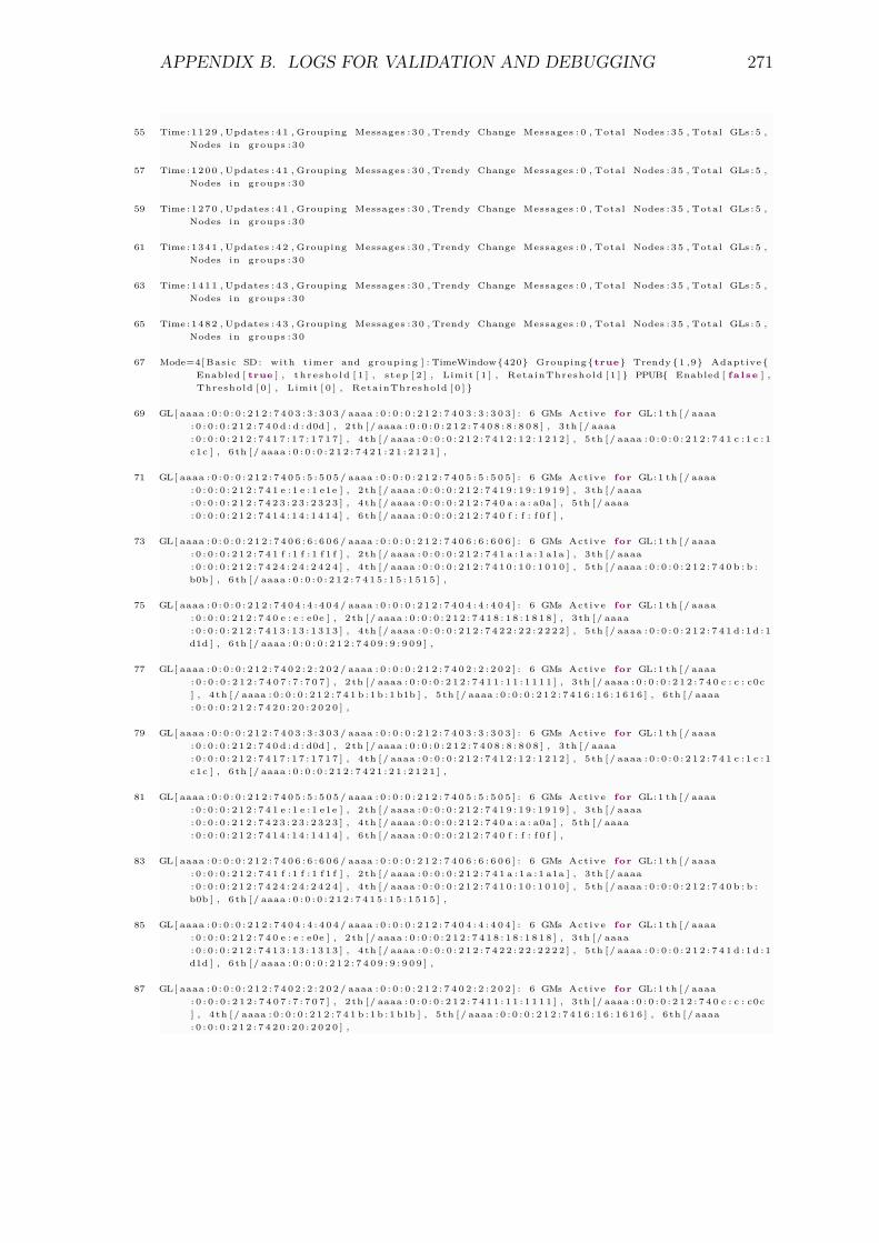
APPENDIX B. LOGS FOR VALIDATION AND DEBUGGING 271
55 Time : 1 1 2 9 , Updates : 4 1 , Grouping Messages : 3 0 , Trendy Change Messages : 0 , Total Nodes : 3 5 , Total GLs : 5 ,Nodes i n groups : 3 0
57 Time : 1 2 0 0 , Updates : 4 1 , Grouping Messages : 3 0 , Trendy Change Messages : 0 , Total Nodes : 3 5 , Total GLs : 5 ,Nodes i n groups : 3 0
59 Time : 1 2 7 0 , Updates : 4 1 , Grouping Messages : 3 0 , Trendy Change Messages : 0 , Total Nodes : 3 5 , Total GLs : 5 ,Nodes i n groups : 3 0
61 Time : 1 3 4 1 , Updates : 4 2 , Grouping Messages : 3 0 , Trendy Change Messages : 0 , Total Nodes : 3 5 , Total GLs : 5 ,Nodes i n groups : 3 0
63 Time : 1 4 1 1 , Updates : 4 3 , Grouping Messages : 3 0 , Trendy Change Messages : 0 , Total Nodes : 3 5 , Total GLs : 5 ,Nodes i n groups : 3 0
65 Time : 1 4 8 2 , Updates : 4 3 , Grouping Messages : 3 0 , Trendy Change Messages : 0 , Total Nodes : 3 5 , Total GLs : 5 ,Nodes i n groups : 3 0
67 Mode=4[ Basic SD : with t imer and grouping ] : TimeWindow{420} Grouping {true} Trendy {1 ,9} Adaptive {Enabled [ true ] , t h r e s h o l d [ 1 ] , s t e p [ 2 ] , Limit [ 1 ] , RetainThreshold [ 1 ] } PPUB{ Enabled [ f a l s e ] ,Threshold [ 0 ] , Limit [ 0 ] , RetainThreshold [ 0 ] }
69 GL[ aaaa : 0 : 0 : 0 : 2 1 2 : 7 4 0 3 : 3 : 3 0 3 / aaaa : 0 : 0 : 0 : 2 1 2 : 7 4 0 3 : 3 : 3 0 3 ] : 6 GMs Active for GL: 1 th [ / aaaa: 0 : 0 : 0 : 2 1 2 : 7 4 0 d : d : d0d ] , 2 th [ / aaaa : 0 : 0 : 0 : 2 1 2 : 7 4 0 8 : 8 : 8 0 8 ] , 3 th [ / aaaa: 0 : 0 : 0 : 2 1 2 : 7 4 1 7 : 1 7 : 1 7 1 7 ] , 4 th [ / aaaa : 0 : 0 : 0 : 2 1 2 : 7 4 1 2 : 1 2 : 1 2 1 2 ] , 5 th [ / aaaa : 0 : 0 : 0 : 2 1 2 : 7 4 1 c : 1 c : 1c1c ] , 6 th [ / aaaa : 0 : 0 : 0 : 2 1 2 : 7 4 2 1 : 2 1 : 2 1 2 1 ] ,
71 GL[ aaaa : 0 : 0 : 0 : 2 1 2 : 7 4 0 5 : 5 : 5 0 5 / aaaa : 0 : 0 : 0 : 2 1 2 : 7 4 0 5 : 5 : 5 0 5 ] : 6 GMs Active for GL: 1 th [ / aaaa: 0 : 0 : 0 : 2 1 2 : 7 4 1 e : 1 e : 1 e1e ] , 2 th [ / aaaa : 0 : 0 : 0 : 2 1 2 : 7 4 1 9 : 1 9 : 1 9 1 9 ] , 3 th [ / aaaa: 0 : 0 : 0 : 2 1 2 : 7 4 2 3 : 2 3 : 2 3 2 3 ] , 4 th [ / aaaa : 0 : 0 : 0 : 2 1 2 : 7 4 0 a : a : a0a ] , 5 th [ / aaaa: 0 : 0 : 0 : 2 1 2 : 7 4 1 4 : 1 4 : 1 4 1 4 ] , 6 th [ / aaaa : 0 : 0 : 0 : 2 1 2 : 7 4 0 f : f : f 0 f ] ,
73 GL[ aaaa : 0 : 0 : 0 : 2 1 2 : 7 4 0 6 : 6 : 6 0 6 / aaaa : 0 : 0 : 0 : 2 1 2 : 7 4 0 6 : 6 : 6 0 6 ] : 6 GMs Active for GL: 1 th [ / aaaa: 0 : 0 : 0 : 2 1 2 : 7 4 1 f : 1 f : 1 f 1 f ] , 2 th [ / aaaa : 0 : 0 : 0 : 2 1 2 : 7 4 1 a : 1 a : 1 a1a ] , 3 th [ / aaaa: 0 : 0 : 0 : 2 1 2 : 7 4 2 4 : 2 4 : 2 4 2 4 ] , 4 th [ / aaaa : 0 : 0 : 0 : 2 1 2 : 7 4 1 0 : 1 0 : 1 0 1 0 ] , 5 th [ / aaaa : 0 : 0 : 0 : 2 1 2 : 7 4 0 b : b :b0b ] , 6 th [ / aaaa : 0 : 0 : 0 : 2 1 2 : 7 4 1 5 : 1 5 : 1 5 1 5 ] ,
75 GL[ aaaa : 0 : 0 : 0 : 2 1 2 : 7 4 0 4 : 4 : 4 0 4 / aaaa : 0 : 0 : 0 : 2 1 2 : 7 4 0 4 : 4 : 4 0 4 ] : 6 GMs Active for GL: 1 th [ / aaaa: 0 : 0 : 0 : 2 1 2 : 7 4 0 e : e : e0e ] , 2 th [ / aaaa : 0 : 0 : 0 : 2 1 2 : 7 4 1 8 : 1 8 : 1 8 1 8 ] , 3 th [ / aaaa: 0 : 0 : 0 : 2 1 2 : 7 4 1 3 : 1 3 : 1 3 1 3 ] , 4 th [ / aaaa : 0 : 0 : 0 : 2 1 2 : 7 4 2 2 : 2 2 : 2 2 2 2 ] , 5 th [ / aaaa : 0 : 0 : 0 : 2 1 2 : 7 4 1 d : 1 d : 1d1d ] , 6 th [ / aaaa : 0 : 0 : 0 : 2 1 2 : 7 4 0 9 : 9 : 9 0 9 ] ,
77 GL[ aaaa : 0 : 0 : 0 : 2 1 2 : 7 4 0 2 : 2 : 2 0 2 / aaaa : 0 : 0 : 0 : 2 1 2 : 7 4 0 2 : 2 : 2 0 2 ] : 6 GMs Active for GL: 1 th [ / aaaa: 0 : 0 : 0 : 2 1 2 : 7 4 0 7 : 7 : 7 0 7 ] , 2 th [ / aaaa : 0 : 0 : 0 : 2 1 2 : 7 4 1 1 : 1 1 : 1 1 1 1 ] , 3 th [ / aaaa : 0 : 0 : 0 : 2 1 2 : 7 4 0 c : c : c0c] , 4 th [ / aaaa : 0 : 0 : 0 : 2 1 2 : 7 4 1 b : 1 b : 1 b1b ] , 5 th [ / aaaa : 0 : 0 : 0 : 2 1 2 : 7 4 1 6 : 1 6 : 1 6 1 6 ] , 6 th [ / aaaa: 0 : 0 : 0 : 2 1 2 : 7 4 2 0 : 2 0 : 2 0 2 0 ] ,
79 GL[ aaaa : 0 : 0 : 0 : 2 1 2 : 7 4 0 3 : 3 : 3 0 3 / aaaa : 0 : 0 : 0 : 2 1 2 : 7 4 0 3 : 3 : 3 0 3 ] : 6 GMs Active for GL: 1 th [ / aaaa: 0 : 0 : 0 : 2 1 2 : 7 4 0 d : d : d0d ] , 2 th [ / aaaa : 0 : 0 : 0 : 2 1 2 : 7 4 0 8 : 8 : 8 0 8 ] , 3 th [ / aaaa: 0 : 0 : 0 : 2 1 2 : 7 4 1 7 : 1 7 : 1 7 1 7 ] , 4 th [ / aaaa : 0 : 0 : 0 : 2 1 2 : 7 4 1 2 : 1 2 : 1 2 1 2 ] , 5 th [ / aaaa : 0 : 0 : 0 : 2 1 2 : 7 4 1 c : 1 c : 1c1c ] , 6 th [ / aaaa : 0 : 0 : 0 : 2 1 2 : 7 4 2 1 : 2 1 : 2 1 2 1 ] ,
81 GL[ aaaa : 0 : 0 : 0 : 2 1 2 : 7 4 0 5 : 5 : 5 0 5 / aaaa : 0 : 0 : 0 : 2 1 2 : 7 4 0 5 : 5 : 5 0 5 ] : 6 GMs Active for GL: 1 th [ / aaaa: 0 : 0 : 0 : 2 1 2 : 7 4 1 e : 1 e : 1 e1e ] , 2 th [ / aaaa : 0 : 0 : 0 : 2 1 2 : 7 4 1 9 : 1 9 : 1 9 1 9 ] , 3 th [ / aaaa: 0 : 0 : 0 : 2 1 2 : 7 4 2 3 : 2 3 : 2 3 2 3 ] , 4 th [ / aaaa : 0 : 0 : 0 : 2 1 2 : 7 4 0 a : a : a0a ] , 5 th [ / aaaa: 0 : 0 : 0 : 2 1 2 : 7 4 1 4 : 1 4 : 1 4 1 4 ] , 6 th [ / aaaa : 0 : 0 : 0 : 2 1 2 : 7 4 0 f : f : f 0 f ] ,
83 GL[ aaaa : 0 : 0 : 0 : 2 1 2 : 7 4 0 6 : 6 : 6 0 6 / aaaa : 0 : 0 : 0 : 2 1 2 : 7 4 0 6 : 6 : 6 0 6 ] : 6 GMs Active for GL: 1 th [ / aaaa: 0 : 0 : 0 : 2 1 2 : 7 4 1 f : 1 f : 1 f 1 f ] , 2 th [ / aaaa : 0 : 0 : 0 : 2 1 2 : 7 4 1 a : 1 a : 1 a1a ] , 3 th [ / aaaa: 0 : 0 : 0 : 2 1 2 : 7 4 2 4 : 2 4 : 2 4 2 4 ] , 4 th [ / aaaa : 0 : 0 : 0 : 2 1 2 : 7 4 1 0 : 1 0 : 1 0 1 0 ] , 5 th [ / aaaa : 0 : 0 : 0 : 2 1 2 : 7 4 0 b : b :b0b ] , 6 th [ / aaaa : 0 : 0 : 0 : 2 1 2 : 7 4 1 5 : 1 5 : 1 5 1 5 ] ,
85 GL[ aaaa : 0 : 0 : 0 : 2 1 2 : 7 4 0 4 : 4 : 4 0 4 / aaaa : 0 : 0 : 0 : 2 1 2 : 7 4 0 4 : 4 : 4 0 4 ] : 6 GMs Active for GL: 1 th [ / aaaa: 0 : 0 : 0 : 2 1 2 : 7 4 0 e : e : e0e ] , 2 th [ / aaaa : 0 : 0 : 0 : 2 1 2 : 7 4 1 8 : 1 8 : 1 8 1 8 ] , 3 th [ / aaaa: 0 : 0 : 0 : 2 1 2 : 7 4 1 3 : 1 3 : 1 3 1 3 ] , 4 th [ / aaaa : 0 : 0 : 0 : 2 1 2 : 7 4 2 2 : 2 2 : 2 2 2 2 ] , 5 th [ / aaaa : 0 : 0 : 0 : 2 1 2 : 7 4 1 d : 1 d : 1d1d ] , 6 th [ / aaaa : 0 : 0 : 0 : 2 1 2 : 7 4 0 9 : 9 : 9 0 9 ] ,
87 GL[ aaaa : 0 : 0 : 0 : 2 1 2 : 7 4 0 2 : 2 : 2 0 2 / aaaa : 0 : 0 : 0 : 2 1 2 : 7 4 0 2 : 2 : 2 0 2 ] : 6 GMs Active for GL: 1 th [ / aaaa: 0 : 0 : 0 : 2 1 2 : 7 4 0 7 : 7 : 7 0 7 ] , 2 th [ / aaaa : 0 : 0 : 0 : 2 1 2 : 7 4 1 1 : 1 1 : 1 1 1 1 ] , 3 th [ / aaaa : 0 : 0 : 0 : 2 1 2 : 7 4 0 c : c : c0c] , 4 th [ / aaaa : 0 : 0 : 0 : 2 1 2 : 7 4 1 b : 1 b : 1 b1b ] , 5 th [ / aaaa : 0 : 0 : 0 : 2 1 2 : 7 4 1 6 : 1 6 : 1 6 1 6 ] , 6 th [ / aaaa: 0 : 0 : 0 : 2 1 2 : 7 4 2 0 : 2 0 : 2 0 2 0 ] ,
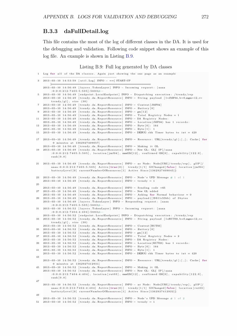
APPENDIX B. LOGS FOR VALIDATION AND DEBUGGING 272
B.3.3 daFullDetail.log
This file contains the most of the log of different classes in the DA. It is used forthe debugging and validation. Following code snippet shows an example of thislog file. An example is shown in Listing B.9.
Listing B.9: Full log generated by DA classes1 Log for a l l o f the DA c l a s s e s . Again j u s t showing the one page as an example
−−−−−−−−−−−−−−−−−−−−−−−−−−−−−−−−−−−−−−−−−−3 2013−03−10 1 4 : 5 3 : 5 9 [ u t i l . Log ] INFO − ==[ START−UP
]========================================================2013−03−10 1 4 : 5 6 : 4 9 [ l a y e r s . TokenLayer ] INFO − Incoming r e q u e s t : [ aaaa
: 0 : 0 : 0 : 2 1 2 : 7 4 0 5 : 5 : 5 0 5 ] : 5 6 8 3#−−5 2013−03−10 1 4 : 5 6 : 4 9 [ endpoint . LocalEndpoint ] INFO − Disp atching e x e c u t i o n : / trendy / rep
2013−03−10 1 4 : 5 6 : 4 9 [ trendy . da . ReportResource ] INFO − S t r i n g payload [ l=JMF04 , b=0,mgm=12 , r=trendy / g l ] , s i z e ( 3 0 )
7 2013−03−10 1 4 : 5 6 : 4 9 [ trendy . da . ReportResource ] INFO − Context [ JMF04 ]2013−03−10 1 4 : 5 6 : 4 9 [ trendy . da . ReportResource ] INFO − Battery [ 0 ]
9 2013−03−10 1 4 : 5 6 : 4 9 [ trendy . da . ReportResource ] INFO − gm [ 1 2 ]2013−03−10 1 4 : 5 6 : 4 9 [ trendy . da . ReportResource ] INFO − Total R e g i s t r y Nodes = 1
11 2013−03−10 1 4 : 5 6 : 4 9 [ trendy . da . ReportResource ] INFO − DA R e g i s t r y Nodes :2013−03−10 1 4 : 5 6 : 4 9 [ trendy . da . ReportResource ] INFO − Locat ion (JMF04) has 1 r e c o r d s :
13 2013−03−10 1 4 : 5 6 : 4 9 [ trendy . da . ReportResource ] INFO − Byte [ 0 ] : 1642013−03−10 1 4 : 5 6 : 4 9 [ trendy . da . ReportResource ] INFO − Byte [ 1 ] : 1
15 2013−03−10 1 4 : 5 6 : 4 9 [ trendy . da . ReportResource ] INFO − DEBUG chk Timer bytes to i n t = 420
17 2013−03−10 1 4 : 5 6 : 4 9 [ trendy . da . ReportResource ] INFO − Resource : URL[ trendy / g l ] ; [ , ] ; Cache [ for0 minutes at 1362927409057]
2013−03−10 1 4 : 5 6 : 4 9 [ trendy . da . ReportResource ] INFO − Making i t GL19 2013−03−10 1 4 : 5 6 : 4 9 [ trendy . da . ReportResource ] INFO − New GL: GL{ IP [ / aaaa
: 0 : 0 : 0 : 2 1 2 : 7 4 0 5 : 5 : 5 0 5 ] , l o c a t i o n [ jmf04 ] , maxGM[ 1 2 ] , conf irmed GM[ 0 ] , c a p a b i l i t y [ 1 2 2 . 0 ] ,rank [ 0 . 0 ]
21 2013−03−10 1 4 : 5 6 : 4 9 [ trendy . da . ReportResource ] INFO − as Node : Node{URI [ / trendy / rep ] , g l I P [ /aaaa : 0 : 0 : 0 : 2 1 2 : 7 4 0 5 : 5 : 5 0 5 ] Active [ true ( 0 ) ] trendy [ 1 / 1 ] GlChanged [ f a l s e ] l o c a t i o n [ jmf04 ]b a t t e r y L e v e l [ 0 ] currentNumberOfResources [ 1 ] Active S i n c e [ 1 3 6 2 9 2 7 4 0 9 0 4 5 ] }
23 2013−03−10 1 4 : 5 6 : 4 9 [ trendy . da . ReportResource ] INFO − Node ’ s UPD Message # 1 o f 12013−03−10 1 4 : 5 6 : 4 9 [ trendy . da . ReportResource ] INFO − trendy = 1
252013−03−10 1 4 : 5 6 : 4 9 [ trendy . da . ReportResource ] INFO − Sending code =65
27 2013−03−10 1 4 : 5 6 : 4 9 [ trendy . da . ReportResource ] INFO − New GL added2013−03−10 1 4 : 5 6 : 4 9 [ trendy . da . ReportResource ] INFO − Asking for Normal behaviour = 0
29 2013−03−10 1 4 : 5 6 : 4 9 [ trendy . da . ReportResource ] INFO − payload ( [ B@11c55bb ) o f 3 bytes2013−03−10 1 4 : 5 6 : 4 9 [ l a y e r s . TokenLayer ] INFO − Responding r e q u e s t : [ aaaa
: 0 : 0 : 0 : 2 1 2 : 7 4 0 5 : 5 : 5 0 5 ] : 5 6 8 3#−−31 2013−03−10 1 4 : 5 6 : 5 2 [ l a y e r s . TokenLayer ] INFO − Incoming r e q u e s t : [ aaaa
: 0 : 0 : 0 : 2 1 2 : 7 4 0 4 : 4 : 4 0 4 ] : 5 6 8 3#−−2013−03−10 1 4 : 5 6 : 5 2 [ endpoint . LocalEndpoint ] INFO − Disp atching e x e c u t i o n : / trendy / rep
33 2013−03−10 1 4 : 5 6 : 5 2 [ trendy . da . ReportResource ] INFO − S t r i n g payload [ l=RUT03, b=0,mgm=12 , r=trendy / g l ] , s i z e ( 3 0 )
2013−03−10 1 4 : 5 6 : 5 2 [ trendy . da . ReportResource ] INFO − Context [ RUT03 ]35 2013−03−10 1 4 : 5 6 : 5 2 [ trendy . da . ReportResource ] INFO − Battery [ 0 ]
2013−03−10 1 4 : 5 6 : 5 2 [ trendy . da . ReportResource ] INFO − gm [ 1 2 ]37 2013−03−10 1 4 : 5 6 : 5 2 [ trendy . da . ReportResource ] INFO − Total R e g i s t r y Nodes = 2
2013−03−10 1 4 : 5 6 : 5 2 [ trendy . da . ReportResource ] INFO − DA R e g i s t r y Nodes :39 2013−03−10 1 4 : 5 6 : 5 2 [ trendy . da . ReportResource ] INFO − Locat ion (RUT03) has 1 r e c o r d s :
2013−03−10 1 4 : 5 6 : 5 2 [ trendy . da . ReportResource ] INFO − Byte [ 0 ] : 16441 2013−03−10 1 4 : 5 6 : 5 2 [ trendy . da . ReportResource ] INFO − Byte [ 1 ] : 1
2013−03−10 1 4 : 5 6 : 5 2 [ trendy . da . ReportResource ] INFO − DEBUG chk Timer bytes to i n t = 42043
2013−03−10 1 4 : 5 6 : 5 2 [ trendy . da . ReportResource ] INFO − Resource : URL[ trendy / g l ] ; [ , ] ; Cache [ for0 minutes at 1362927412931]
45 2013−03−10 1 4 : 5 6 : 5 2 [ trendy . da . ReportResource ] INFO − Making i t GL2013−03−10 1 4 : 5 6 : 5 2 [ trendy . da . ReportResource ] INFO − New GL: GL{ IP [ / aaaa
: 0 : 0 : 0 : 2 1 2 : 7 4 0 4 : 4 : 4 0 4 ] , l o c a t i o n [ rut03 ] , maxGM[ 1 2 ] , conf irmed GM[ 0 ] , c a p a b i l i t y [ 1 2 2 . 0 ] ,rank [ 0 . 0 ]
472013−03−10 1 4 : 5 6 : 5 2 [ trendy . da . ReportResource ] INFO − as Node : Node{URI [ / trendy / rep ] , g l I P [ /
aaaa : 0 : 0 : 0 : 2 1 2 : 7 4 0 4 : 4 : 4 0 4 ] Active [ true ( 0 ) ] trendy [ 1 / 1 ] GlChanged [ f a l s e ] l o c a t i o n [ rut03 ]b a t t e r y L e v e l [ 0 ] currentNumberOfResources [ 1 ] Active S i n c e [ 1 3 6 2 9 2 7 4 1 2 9 2 2 ] }
492013−03−10 1 4 : 5 6 : 5 2 [ trendy . da . ReportResource ] INFO − Node ’ s UPD Message # 1 o f 2
51 2013−03−10 1 4 : 5 6 : 5 2 [ trendy . da . ReportResource ] INFO − trendy = 1
APPENDIX B. LOGS FOR VALIDATION AND DEBUGGING 273
53 2013−03−10 1 4 : 5 6 : 5 2 [ trendy . da . ReportResource ] INFO − Sending code =652013−03−10 1 4 : 5 6 : 5 2 [ trendy . da . ReportResource ] INFO − New GL added
55 2013−03−10 1 4 : 5 6 : 5 2 [ trendy . da . ReportResource ] INFO − Asking for Normal behaviour = 02013−03−10 1 4 : 5 6 : 5 2 [ trendy . da . ReportResource ] INFO − payload ( [ B@1d31859 ) o f 3 bytes
57 2013−03−10 1 4 : 5 6 : 5 2 [ l a y e r s . TokenLayer ] INFO − Responding r e q u e s t : [ aaaa: 0 : 0 : 0 : 2 1 2 : 7 4 0 4 : 4 : 4 0 4 ] : 5 6 8 3#−−
2013−03−10 1 4 : 5 6 : 5 7 [ l a y e r s . TokenLayer ] INFO − Incoming r e q u e s t : [ aaaa: 0 : 0 : 0 : 2 1 2 : 7 4 0 2 : 2 : 2 0 2 ] : 5 6 8 3#−−
59 2013−03−10 1 4 : 5 6 : 5 7 [ endpoint . LocalEndpoint ] INFO − Disp atching e x e c u t i o n : / trendy / rep2013−03−10 1 4 : 5 6 : 5 7 [ trendy . da . ReportResource ] INFO − S t r i n g payload [ l=INB01 , b=0,mgm=12 , r=
trendy / g l ] , s i z e ( 3 0 )61 2013−03−10 1 4 : 5 6 : 5 7 [ trendy . da . ReportResource ] INFO − Context [ INB01 ]
2013−03−10 1 4 : 5 6 : 5 7 [ trendy . da . ReportResource ] INFO − Battery [ 0 ]63 2013−03−10 1 4 : 5 6 : 5 7 [ trendy . da . ReportResource ] INFO − gm [ 1 2 ]
2013−03−10 1 4 : 5 6 : 5 7 [ trendy . da . ReportResource ] INFO − Total R e g i s t r y Nodes = 365 2013−03−10 1 4 : 5 6 : 5 7 [ trendy . da . ReportResource ] INFO − DA R e g i s t r y Nodes :
2013−03−10 1 4 : 5 6 : 5 7 [ trendy . da . ReportResource ] INFO − Locat ion ( INB01 ) has 1 r e c o r d s :67 2013−03−10 1 4 : 5 6 : 5 7 [ trendy . da . ReportResource ] INFO − Byte [ 0 ] : 164
2013−03−10 1 4 : 5 6 : 5 7 [ trendy . da . ReportResource ] INFO − Byte [ 1 ] : 169 2013−03−10 1 4 : 5 6 : 5 7 [ trendy . da . ReportResource ] INFO − DEBUG chk Timer bytes to i n t = 420
71 2013−03−10 1 4 : 5 6 : 5 7 [ trendy . da . ReportResource ] INFO − Resource : URL[ trendy / g l ] ; [ , ] ; Cache [ for0 minutes at 1362927417711]
2013−03−10 1 4 : 5 6 : 5 7 [ trendy . da . ReportResource ] INFO − Making i t GL73 2013−03−10 1 4 : 5 6 : 5 7 [ trendy . da . ReportResource ] INFO − New GL: GL{ IP [ / aaaa
: 0 : 0 : 0 : 2 1 2 : 7 4 0 2 : 2 : 2 0 2 ] , l o c a t i o n [ inb01 ] , maxGM[ 1 2 ] , conf irmed GM[ 0 ] , c a p a b i l i t y [ 1 2 2 . 0 ] ,rank [ 0 . 0 ]
75 2013−03−10 1 4 : 5 6 : 5 7 [ trendy . da . ReportResource ] INFO − as Node : Node{URI [ / trendy / rep ] , g l I P [ /aaaa : 0 : 0 : 0 : 2 1 2 : 7 4 0 2 : 2 : 2 0 2 ] Active [ true ( 0 ) ] trendy [ 1 / 1 ] GlChanged [ f a l s e ] l o c a t i o n [ inb01 ]b a t t e r y L e v e l [ 0 ] currentNumberOfResources [ 1 ] Active S i n c e [ 1 3 6 2 9 2 7 4 1 7 7 0 3 ] }
77 2013−03−10 1 4 : 5 6 : 5 7 [ trendy . da . ReportResource ] INFO − Node ’ s UPD Message # 1 o f 32013−03−10 1 4 : 5 6 : 5 7 [ trendy . da . ReportResource ] INFO − trendy = 1
792013−03−10 1 4 : 5 6 : 5 7 [ trendy . da . ReportResource ] INFO − Sending code =65
81 2013−03−10 1 4 : 5 6 : 5 7 [ trendy . da . ReportResource ] INFO − New GL added2013−03−10 1 4 : 5 6 : 5 7 [ trendy . da . ReportResource ] INFO − Asking for Normal behaviour = 0
83 2013−03−10 1 4 : 5 6 : 5 7 [ trendy . da . ReportResource ] INFO − payload ( [ B@15a07bf ) o f 3 bytes2013−03−10 1 4 : 5 6 : 5 7 [ l a y e r s . TokenLayer ] INFO − Responding r e q u e s t : [ aaaa
: 0 : 0 : 0 : 2 1 2 : 7 4 0 2 : 2 : 2 0 2 ] : 5 6 8 3#−−85 2013−03−10 1 4 : 5 7 : 0 5 [ l a y e r s . TokenLayer ] INFO − Incoming r e q u e s t : [ aaaa
: 0 : 0 : 0 : 2 1 2 : 7 4 0 6 : 6 : 6 0 6 ] : 5 6 8 3#−−2013−03−10 1 4 : 5 7 : 0 5 [ endpoint . LocalEndpoint ] INFO − Disp atching e x e c u t i o n : / trendy / rep
87 2013−03−10 1 4 : 5 7 : 0 5 [ trendy . da . ReportResource ] INFO − S t r i n g payload [ l=SSB05 , b=0,mgm=12 , r=trendy / g l ] , s i z e ( 3 0 )
2013−03−10 1 4 : 5 7 : 0 5 [ trendy . da . ReportResource ] INFO − Context [ SSB05 ]89 2013−03−10 1 4 : 5 7 : 0 5 [ trendy . da . ReportResource ] INFO − Battery [ 0 ]
2013−03−10 1 4 : 5 7 : 0 5 [ trendy . da . ReportResource ] INFO − gm [ 1 2 ]91 2013−03−10 1 4 : 5 7 : 0 5 [ trendy . da . ReportResource ] INFO − Total R e g i s t r y Nodes = 4
2013−03−10 1 4 : 5 7 : 0 5 [ trendy . da . ReportResource ] INFO − DA R e g i s t r y Nodes :93 2013−03−10 1 4 : 5 7 : 0 5 [ trendy . da . ReportResource ] INFO − Locat ion ( SSB05 ) has 1 r e c o r d s :
2013−03−10 1 4 : 5 7 : 0 5 [ trendy . da . ReportResource ] INFO − Byte [ 0 ] : 16495 2013−03−10 1 4 : 5 7 : 0 5 [ trendy . da . ReportResource ] INFO − Byte [ 1 ] : 1
2013−03−10 1 4 : 5 7 : 0 5 [ trendy . da . ReportResource ] INFO − DEBUG chk Timer bytes to i n t = 42097
2013−03−10 1 4 : 5 7 : 0 5 [ trendy . da . ReportResource ] INFO − Resource : URL[ trendy / g l ] ; [ , ] ; Cache [ for0 minutes at 1362927425199]
99 2013−03−10 1 4 : 5 7 : 0 5 [ trendy . da . ReportResource ] INFO − Making i t GL2013−03−10 1 4 : 5 7 : 0 5 [ trendy . da . ReportResource ] INFO − New GL: GL{ IP [ / aaaa
: 0 : 0 : 0 : 2 1 2 : 7 4 0 6 : 6 : 6 0 6 ] , l o c a t i o n [ ssb05 ] , maxGM[ 1 2 ] , conf irmed GM[ 0 ] , c a p a b i l i t y [ 1 2 2 . 0 ] ,rank [ 0 . 0 ]
1012013−03−10 1 4 : 5 7 : 0 5 [ trendy . da . ReportResource ] INFO − as Node : Node{URI [ / trendy / rep ] , g l I P [ /
aaaa : 0 : 0 : 0 : 2 1 2 : 7 4 0 6 : 6 : 6 0 6 ] Active [ true ( 0 ) ] trendy [ 1 / 1 ] GlChanged [ f a l s e ] l o c a t i o n [ ssb05 ]b a t t e r y L e v e l [ 0 ] currentNumberOfResources [ 1 ] Active S i n c e [ 1 3 6 2 9 2 7 4 2 5 1 8 9 ] }
1032013−03−10 1 4 : 5 7 : 0 5 [ trendy . da . ReportResource ] INFO − Node ’ s UPD Message # 1 o f 4
105 2013−03−10 1 4 : 5 7 : 0 5 [ trendy . da . ReportResource ] INFO − trendy = 1
107 2013−03−10 1 4 : 5 7 : 0 5 [ trendy . da . ReportResource ] INFO − Sending code =652013−03−10 1 4 : 5 7 : 0 5 [ trendy . da . ReportResource ] INFO − New GL added
109 2013−03−10 1 4 : 5 7 : 0 5 [ trendy . da . ReportResource ] INFO − Asking for Normal behaviour = 02013−03−10 1 4 : 5 7 : 0 5 [ trendy . da . ReportResource ] INFO − payload ( [ B@8f3d27 ) o f 3 bytes
111 2013−03−10 1 4 : 5 7 : 0 5 [ l a y e r s . TokenLayer ] INFO − Responding r e q u e s t : [ aaaa: 0 : 0 : 0 : 2 1 2 : 7 4 0 6 : 6 : 6 0 6 ] : 5 6 8 3#−−
2013−03−10 1 4 : 5 7 : 1 4 [ l a y e r s . TokenLayer ] INFO − Incoming r e q u e s t : [ aaaa: 0 : 0 : 0 : 2 1 2 : 7 4 0 3 : 3 : 3 0 3 ] : 5 6 8 3#−−
113 2013−03−10 1 4 : 5 7 : 1 4 [ endpoint . LocalEndpoint ] INFO − Disp atching e x e c u t i o n : / trendy / rep
APPENDIX B. LOGS FOR VALIDATION AND DEBUGGING 274
2013−03−10 1 4 : 5 7 : 1 4 [ trendy . da . ReportResource ] INFO − S t r i n g payload [ l=HSG02 , b=0,mgm=12 , r=trendy / g l ] , s i z e ( 3 0 )
115 2013−03−10 1 4 : 5 7 : 1 4 [ trendy . da . ReportResource ] INFO − Context [ HSG02 ]2013−03−10 1 4 : 5 7 : 1 4 [ trendy . da . ReportResource ] INFO − Battery [ 0 ]
117 2013−03−10 1 4 : 5 7 : 1 4 [ trendy . da . ReportResource ] INFO − gm [ 1 2 ]2013−03−10 1 4 : 5 7 : 1 4 [ trendy . da . ReportResource ] INFO − Total R e g i s t r y Nodes = 5
119 2013−03−10 1 4 : 5 7 : 1 4 [ trendy . da . ReportResource ] INFO − DA R e g i s t r y Nodes :2013−03−10 1 4 : 5 7 : 1 4 [ trendy . da . ReportResource ] INFO − Locat ion (HSG02) has 1 r e c o r d s :
121 2013−03−10 1 4 : 5 7 : 1 4 [ trendy . da . ReportResource ] INFO − Byte [ 0 ] : 1642013−03−10 1 4 : 5 7 : 1 4 [ trendy . da . ReportResource ] INFO − Byte [ 1 ] : 1
123 2013−03−10 1 4 : 5 7 : 1 4 [ trendy . da . ReportResource ] INFO − DEBUG chk Timer bytes to i n t = 420
125 2013−03−10 1 4 : 5 7 : 1 4 [ trendy . da . ReportResource ] INFO − Resource : URL[ trendy / g l ] ; [ , ] ; Cache [ for0 minutes at 1362927434372]
2013−03−10 1 4 : 5 7 : 1 4 [ trendy . da . ReportResource ] INFO − Making i t GL127 2013−03−10 1 4 : 5 7 : 1 4 [ trendy . da . ReportResource ] INFO − New GL: GL{ IP [ / aaaa
: 0 : 0 : 0 : 2 1 2 : 7 4 0 3 : 3 : 3 0 3 ] , l o c a t i o n [ hsg02 ] , maxGM[ 1 2 ] , conf irmed GM[ 0 ] , c a p a b i l i t y [ 1 2 2 . 0 ] ,rank [ 0 . 0 ]
129 2013−03−10 1 4 : 5 7 : 1 4 [ trendy . da . ReportResource ] INFO − as Node : Node{URI [ / trendy / rep ] , g l I P [ /aaaa : 0 : 0 : 0 : 2 1 2 : 7 4 0 3 : 3 : 3 0 3 ] Active [ true ( 0 ) ] trendy [ 1 / 1 ] GlChanged [ f a l s e ] l o c a t i o n [ hsg02 ]b a t t e r y L e v e l [ 0 ] currentNumberOfResources [ 1 ] Active S i n c e [ 1 3 6 2 9 2 7 4 3 4 3 6 3 ] }
131 2013−03−10 1 4 : 5 7 : 1 4 [ trendy . da . ReportResource ] INFO − Node ’ s UPD Message # 1 o f 52013−03−10 1 4 : 5 7 : 1 4 [ trendy . da . ReportResource ] INFO − trendy = 1
1332013−03−10 1 4 : 5 7 : 1 4 [ trendy . da . ReportResource ] INFO − Sending code =65
135 2013−03−10 1 4 : 5 7 : 1 4 [ trendy . da . ReportResource ] INFO − New GL added2013−03−10 1 4 : 5 7 : 1 4 [ trendy . da . ReportResource ] INFO − Asking for Normal behaviour = 0
137 2013−03−10 1 4 : 5 7 : 1 4 [ trendy . da . ReportResource ] INFO − payload ( [ B@1e6f0ef ) o f 3 bytes2013−03−10 1 4 : 5 7 : 1 4 [ l a y e r s . TokenLayer ] INFO − Responding r e q u e s t : [ aaaa
: 0 : 0 : 0 : 2 1 2 : 7 4 0 3 : 3 : 3 0 3 ] : 5 6 8 3#−−139 2013−03−10 1 4 : 5 7 : 2 0 [ l a y e r s . TokenLayer ] INFO − Incoming r e q u e s t : [ aaaa : 0 : 0 : 0 : 2 1 2 : 7 4 0 e : e : e0e
] : 5 6 8 3#−−2013−03−10 1 4 : 5 7 : 2 0 [ endpoint . LocalEndpoint ] INFO − Disp atching e x e c u t i o n : / trendy / rep
141 2013−03−10 1 4 : 5 7 : 2 0 [ trendy . da . ReportResource ] INFO − S t r i n g payload [ l=RUT03, b=0, r=l i g h t ;humid ; temp ; ] , s i z e ( 3 1 )
2013−03−10 1 4 : 5 7 : 2 0 [ trendy . da . ReportResource ] INFO − Context [ RUT03 ]143 2013−03−10 1 4 : 5 7 : 2 0 [ trendy . da . ReportResource ] INFO − Battery [ 0 ]
2013−03−10 1 4 : 5 7 : 2 0 [ trendy . da . ReportResource ] INFO − Total R e g i s t r y Nodes = 5145 2013−03−10 1 4 : 5 7 : 2 0 [ trendy . da . ReportResource ] INFO − DA R e g i s t r y Nodes :
2013−03−10 1 4 : 5 7 : 2 0 [ trendy . da . ReportResource ] INFO − Locat ion (RUT03) has 2 r e c o r d s :147 2013−03−10 1 4 : 5 7 : 2 0 [ trendy . da . ReportResource ] INFO − Byte [ 0 ] : 164
2013−03−10 1 4 : 5 7 : 2 0 [ trendy . da . ReportResource ] INFO − Byte [ 1 ] : 1149 2013−03−10 1 4 : 5 7 : 2 0 [ trendy . da . ReportResource ] INFO − DEBUG chk Timer bytes to i n t = 420
B.4 UA Log
The UA generates following log files:
B.4.1 uaperformance-processed.log
It contains very general information about the results, which is used for graphsafter some processing. An example is shown in Listing B.10.
Listing B.10: UA log for graph generation after further processing1 Format :
Query#3 S e r v i c e Discovery delay :
S e r v i c e i n v o c a t i o n delay :5 Optimal S e r v i c e s e l e c t i o n :
Group query :7 −−−−−−−−−−−−−−−−−−−−−−−−−−−−−
1 21.507398 576.7593153500001 1 09 2 19.485132 500.78959975 1 0
3 14.615253 687.337319 1 011 4 17.641199 319.83119405 1 0
5 16.978385 527.99205795 1 0
APPENDIX B. LOGS FOR VALIDATION AND DEBUGGING 275
13 6 20.059484 347.14612509999995 1 07 22.514677 1287.6573075 1 0
15 8 14.014749 1084.5305371499999 1 09 23.075649 572.03808725 1 0
17 10 23.555236 428.37224069999996 1 0
B.4.2 ua-detail.log
This file holds some details about the status of the UA including the details ofqueries and responses. An example is shown in Listing B.11.
Listing B.11: Full UA log including detail of queries and responses−−−−−−−−−−−−−−−−−−−−−−−−−−−−−−−−−−−−−−−−−−−−−−−−−−−−−−−−−−−−−−−−−−−−−−−−−−−−−−−−−
2 2013/03/10 1 4 : 5 8 : 5 9Query [ l o c a t i o n=INB01&type=humid ] : Response#1 : aaaa : 0 : 0 : 0 : 2 1 2 : 7 4 1 6 : 1 6 : 1 6 1 6 ; / humid ; r t =; i n f o =; ,
4Query [ l o c a t i o n=INB01&type=humid ] : Response#1 : { 2 3 7 : 7 9 5 } 3 0
6Time : 1 , I n t e r v a l : 1 s e c s , Query#: 1 , INB01 , S e r v i c e Discovery Delay : 2 1 . 5 0 7 3 9 8 , S e r v i c e I n v o c a t i o n
Delay : 6 7 8 . 5 4 0 3 7 1 , Optimal S e r v i c e S e l e c t i o n : true , Group S e r v i c e S e l e c t i o n : f a l s e8
Query [ l o c a t i o n=INB01&i n f o=l i g h t ] : Response#2 : aaaa : 0 : 0 : 0 : 2 1 2 : 7 4 1 6 : 1 6 : 1 6 1 6 ; / l i g h t ; r t =; i n f o =; ,10
Query [ l o c a t i o n=INB01&i n f o=l i g h t ] : Response#2 : { 7 1 : 2 6 2 } 1 012
Time : 9 , I n t e r v a l : 7 s e c s , Query#: 2 , INB01 , S e r v i c e Discovery Delay : 1 9 . 4 8 5 1 3 2 , S e r v i c e I n v o c a t i o nDelay : 5 8 9 . 1 6 4 2 3 5 , Optimal S e r v i c e S e l e c t i o n : true , Group S e r v i c e S e l e c t i o n : f a l s e
14Query [ l o c a t i o n=INB01&i n f o=l i g h t ] : Response#3 : aaaa : 0 : 0 : 0 : 2 1 2 : 7 4 1 6 : 1 6 : 1 6 1 6 ; / l i g h t ; r t =; i n f o =; ,
16Query [ l o c a t i o n=INB01&i n f o=l i g h t ] : Response#3 : { 3 2 8 : 1 0 2 5 } 1 0
18Time : 1 7 , I n t e r v a l : 7 s e c s , Query#: 3 , INB01 , S e r v i c e Discovery Delay : 1 4 . 6 1 5 2 5 3 , S e r v i c e I n v o c a t i o n
Delay : 8 0 8 . 6 3 2 1 4 , Optimal S e r v i c e S e l e c t i o n : true , Group S e r v i c e S e l e c t i o n : f a l s e20
Query [ l o c a t i o n=HSG02&i n f o=humid ] : Response#4 : aaaa : 0 : 0 : 0 : 2 1 2 : 7 4 2 1 : 2 1 : 2 1 2 1 ; / humid ; r t =; i n f o =; ,22
Query [ l o c a t i o n=HSG02&i n f o=humid ] : Response#4 : { 2 5 7 : 7 9 5 } 3 024
Time : 2 3 , I n t e r v a l : 6 s e c s , Query#: 4 , HSG02 , S e r v i c e Discovery Delay : 1 7 . 6 4 1 1 9 9 , S e r v i c e I n v o c a t i o nDelay : 3 7 6 . 2 7 1 9 9 3 , Optimal S e r v i c e S e l e c t i o n : true , Group S e r v i c e S e l e c t i o n : f a l s e
26Query [ l o c a t i o n=RUT03&type=l&i n f o=l i g h t ] : Response#5 : aaaa : 0 : 0 : 0 : 2 1 2 : 7 4 0 9 : 9 : 9 0 9 ; / l i g h t ; r t =; i n f o
=; ,28
Query [ l o c a t i o n=RUT03&type=l&i n f o=l i g h t ] : Response#5 : { 2 8 0 : 8 6 9 } 1 0
Appendix C
Automation for statisticsprocessing and graph generation
This chapter covers the detail of automation of raw statistics processing and thegeneration of graphs.
C.1 Data Processing
A bash script is written to process all the collected raw log files generated by thesimulations to calculate the means and standard deviations for a set of experiments.Listing C.1 presents the code.
Listing C.1: Bash Script to process generated log files for mean and standarddeviation values#! / bin / bash
2noOfArgumentsReqd =3;
4 i f [ " $#" −ne " $noOfArgumentsReqd " ] ; thenecho " Usage : Need $noOfArgumentsReqd arguments "
6 exit 1f i
8totalSimTime=$1
10 t o p o l o g i e s=$2numOfQueryVariations=$3
12i f [ " $4 " == " " ] ; then
14 numOfCases=4echo " Number o f Cases : $numOfCases "
16 e l s enumOfCases=$4
18 echo " Number o f Cases : $numOfCases "f i
20i f [ " $5 " == " " ] ; then
22 bFDIR=$PWDecho " D i r e c t o r y f o r : $bFDIR "
24 e l s ebFDIR=$5
26 echo " D i r e c t o r y f o r : $bFDIR "f i
28c l e a n A l l R e s u l t s=" " ;
30 c l e a n I n d R e s u l t s=" " ;c l e an U a R e s u lt s=" " ;
276
APPENDIX C. AUTOMATION FOR STATISTICS AND GRAPHS 277
32 c leanDaResults=" " ;
34 #C o n f i g u r i n g a t t r i b u t e sfor ( ( i = 1 ; i <= $ t o p o l o g i e s ; i ++)) ; do
36 case " $ i " i n
38 " 1 " )tFDIR=$bFDIR/ " top1 " ;
40 ; ;" 2 " )
42 tFDIR=$bFDIR/ " top2 " ;; ;
44 " 3 " )tFDIR=$bFDIR/ " top3 " ;
46 ; ;∗)
48 echo " Ending "; ;
50 e s a cfor ( ( j = 1 ; j <= $numOfQueryVariations ; j++)) ; do
52case " $ j " i n
54" 1 " )
56 qFDIR=$tFDIR/ " q100 " ;numberOfQueries =100;
58 ; ;" 2 " )
60 qFDIR=$tFDIR/ " q1000 " ;numberOfQueries =1000;
62 ; ;∗)
64 echo " Ending "; ;
66 e s a c
68 #−−−−−−−−−−−−−−−−−−−−P r o c e s s i n g f o r each case−−−−−−−−−−−−−−−−−−−−−−−−−−−for ( ( k = 1 ; k <= $numOfCases ; k++)) ; do
70NUMBEROFNODES=35
72 SIMNAMEFORMATTED=" case−$k "
74 gFDIR=$qFDIR ;cd $gFDIR
76 echo " D i r e c t o r y : $gFDIR case−$k : P r e s s e e n t e r to c o n t i n u e " ; #read l i n e
78 # Creat ing d i r e c t o r i e sg n u r e s u l t s=$gFDIR " /gnu− f i l e s "
80 mkdir −p $ g n u r e s u l t s
82 a l l g n u r e s u l t s=$ g n u r e s u l t s " / a l l "mkdir −p $ a l l g n u r e s u l t s
84i n d g n u r e s u l t s=$ g n u r e s u l t s " / ind "
86 mkdir −p $ i n d g n u r e s u l t s
88 u a g n u r e s u l t s=$ g n u r e s u l t s " /ua "mkdir −p $ u a g n u r e s u l t s
90d a g n u r e s u l t s=$ g n u r e s u l t s " /da "
92 mkdir −p $ d a g n u r e s u l t s
94 a r e s u l t s=$gFDIR " / a l l "mkdir −p $ a r e s u l t s
96 echo " Created : " $ a r e s u l t sc l e a n A l l R e s u l t s=" $ a r e s u l t s " ;
98a m r e s u l t s=$ a r e s u l t s " /mean "
100 mkdir −p $ a m r e s u l t s
102 i r e s u l t s=$gFDIR " / ind "mkdir −p $ i r e s u l t s
104 c l e a n I n d R e s u l t s=" $ i r e s u l t s " ;
106 i d r e s u l t s=$ i r e s u l t s " / i n d i "mkdir −p $ i d r e s u l t s
108i d s r e s u l t s=$ i r e s u l t s " / s e l e c t e d "
110 mkdir −p $ i d s r e s u l t s
APPENDIX C. AUTOMATION FOR STATISTICS AND GRAPHS 278
112 i m r r e s u l t s=$ i r e s u l t s " /mean−raw "mkdir −p $ i m r r e s u l t s
114i m r e s u l t s=$ i r e s u l t s " /mean "
116 mkdir −p $ i m r e s u l t s
118 i a g m r r e s u l t s=$ i r e s u l t s " /mean−aggr "mkdir −p $ i a g m r r e s u l t s
120u a r e s u l t s=$gFDIR " /ua "
122 mkdir −p $ u a r e s u l t sc l e an U a R e s u lt s=" $ u a r e s u l t s " ;
124u a m r r e s u l t s=$ u a r e s u l t s " /mean−raw "
126 mkdir −p $ u a m r r e s u l t s
128 uamresults=$ u a r e s u l t s " /mean "mkdir −p $uamresults
130uamaresults=$ u a r e s u l t s " /mean−aggr "
132 mkdir −p $uamaresults
134 d a r e s u l t s=$gFDIR " /da "mkdir −p $ d a r e s u l t s
136 c leanDaResults=" $ d a r e s u l t s " ;
138 damresults=$ d a r e s u l t s " /mean "mkdir −p $damresults
140damaresults=$ d a r e s u l t s " /mean−aggr "
142 mkdir −p $damaresults
144 #−−−−−−−−−−−−−−−−P r o c e s s i n g s t a r t e d −−−−−−−−−−−−−−−
146 LOGENERGYALL=$SIMNAMEFORMATTED"−energy−a l l "LOGPACKETALL=$SIMNAMEFORMATTED"−packet−a l l "
148 LOGENERGYIND=$SIMNAMEFORMATTED"−energy−ind "LOGPACKETIND=$SIMNAMEFORMATTED"−packet−ind "
150 LOGUA=$SIMNAMEFORMATTED"−uaperformance−p r o c e s s e d "LOGDA=$SIMNAMEFORMATTED"−daperformance "
152echo " S e p a r a t i n g f i l e s w. r . t . time : P r e s s e e n t e r to c o n t i n u e " ;
154awk −v " l e a l l =$LOGENERGYALL" −F " " ’{ c l o s e ( f ) ; f=$1 }{ p r i n t > " a l l / " f "−" l e a l l " . l o g " } ’
$LOGENERGYALL’ . dat ’156 awk −v " l p a l l=$LOGPACKETALL" −F " " ’{ c l o s e ( f ) ; f=$1 }{ p r i n t > " a l l / " f "−" l p a l l " . l o g " } ’
$LOGPACKETALL’ . dat ’awk −v " l e i n d=$LOGENERGYIND" −F " " ’{ c l o s e ( f ) ; f=$1 }{ p r i n t > " ind / " f "−" l e i n d " . l o g " } ’
$LOGENERGYIND’ . dat ’158 awk −v " l p i n d=$LOGPACKETIND" −F " " ’{ c l o s e ( f ) ; f=$1 }{ p r i n t > " ind / " f "−" l p i n d " . l o g " } ’
$LOGPACKETIND’ . dat ’
160 #echo " Have you s e l e c t e d i n d i v i d u a l f i l e s ? : P r e s s e e n t e r to c o n t i n u e " ; read l i n ecp −f $ i r e s u l t s " / $totalSimTime−" ∗ " . l o g " $ i d s r e s u l t s
162awk −v " l e i n d=$LOGENERGYIND" −F " " ’{ c l o s e ( f ) ; f=$2 ; t=$1 }{ p r i n t > " ind / i n d i / " t "−" l e i n d "−
" f " . l o g " } ’ ’ ind / s e l e c t e d / ’∗ ’ − ’$LOGENERGYIND’ . log ’164 awk −v " l p i n d=$LOGPACKETIND" −F " " ’{ c l o s e ( f ) ; f=$2 ; t=$1 }{ p r i n t > " ind / i n d i / " t "−" l p i n d "−
" f " . l o g " } ’ ’ ind / s e l e c t e d / ’∗ ’ − ’$LOGPACKETIND’ . log ’
166 awk −v " logua=$LOGUA" −F " " ’{ c l o s e ( f ) ; f=$1 }{ p r i n t > " ua/ " logua "−" f " . l o g " } ’ $LOGUA’ . log ’awk −v " logda=$LOGDA" −F " " ’{ c l o s e ( f ) ; f=$1 }{ p r i n t > " da/ " logda "−" f " . l o g " } ’ $LOGDA’ . log ’
168#−−−−−−−−−−−−−−−−Aggregated energy and packet s t a t i s t i c s −−−−−−−−−−−−−−−
170 FILES=$ a r e s u l t s /∗ " case−$k " ∗for f i leName i n $FILES
172 do
174 f i l e =$fi leNames=$fi leName
176 f i l e c =${ s##∗/}f i l e =${ f i l e c %. l o g }
178echo " Going to p r o c e s s : " $ f i l e
180awk −v " simnamef "=$SIMNAMEFORMATTED −v " f i l e t o p r o c e s s=$ f i l e " −v " i s g r o u p i n g=$ i s g r o u p i n g " ’{
182cVal=$2 ;
184a r r [NR]= cVal ;

APPENDIX C. AUTOMATION FOR STATISTICS AND GRAPHS 279
186 i f (NR==1) {min=max=cVal }i f ( cVal>max) {max=cVal }
188 i f ( cVal<min ) {min=cVal }t o t+=cVal ;
190a s o r t ( a r r )
192 mid= (NR/2) +0.5;i f ( ( mid%1)!=0) {
194 mid= i n t ( mid ) ;med=( a r r [ mid]+ a r r [ mid +1]) /2
196 } e l s e {med=a r r [ mid ]
198 }
200 for ( i =1; i<=NF; i ++){a l l n o d e s v a l u e s [ i ]= ( $ i ) ; #populate the array data
202 sum [ i ]=sum [ i ] + ( $ i ) ;
204 }for ( i =1; i<=NF; i ++){
206 mean [ i ]=sum [ i ] / (NR) ;}
208 for ( i =1; i<=NF; i ++){sumsq [ i ]=sumsq [ i ] + ( ( $ i )−mean [ i ] ) ^2 ;
210 }} END {
212p r i n t simnamef " \ t " mean [ 2 ] " \ t " s q r t ( sumsq [ 2 ] / (NR) ) " \ t " min " \ t "max" \ t "med " \ t " mean [ 3 ] " \ t " mean [ 4 ]
" \ t " mean [ 5 ] " \ t " mean [ 6 ] " \ t " mean [ 7 ] " \ t "NR > " a l l /mean/ " f i l e t o p r o c e s s "−mean−stdev . l o g " ;214
} ’ ’ a l l / ’ ${ f i l e } ’ . log ’216
218 #∗− a l l −energy−mean . l o g : [ 1 ] Time : [ 2 , 3 ] Total−E−mean : stdev [ 4 , 5 ] E−CPU : stdev [ 6 , 7 ] E−LPM : stdev[ 8 , 9 ] E−L i s t e n : stdev [ 1 0 , 1 1 ] E−Transmit : stdev
#∗− a l l −packet−mean . logTime : [ 2 , 3 ] Total−Packets−mean : stdev [ 4 , 5 ]UPD : stdev [ 6 , 7 ]GRP : stdev220
done #a l l222
#−−−−−−−−−−−−−−−−I n d i v i d u a l node energy and packet s t a t i s t i c s −−−−−−−−−−−−−−−224 FILES=$ i d r e s u l t s /∗ " $totalSimTime " ∗ " case−$k " ∗
for f i leName i n $FILES226 do
228 f i l e =$fi leNames=$fi leName
230 f i l e c =${ s##∗/}f i l e =${ f i l e c %. l o g }
232echo " Going to p r o c e s s : " $ f i l e
234 echo " P r e s s e e n t e r to c o n t i n u e " ;thisFILENAME=$ f i l e
236awk −v " simnamef "=$SIMNAMEFORMATTED −v " f i l e t o p r o c e s s=$thisFILENAME " −v " i s g r o u p i n g=
$ i s g r o u p i n g " ’{238
cVal=$3 ;240
a r r [NR]= cVal ;242 i f (NR==1) {min=max=cVal }
i f ( cVal>max) {max=cVal }244 i f ( cVal<min ) {min=cVal }
t o t+=cVal ;246
a s o r t ( a r r )248 mid= (NR/2) +0.5;
i f ( ( mid%1)!=0) {250 mid= i n t ( mid ) ;
med=( a r r [ mid]+ a r r [ mid +1]) /2252 } e l s e {
med=a r r [ mid ]254 }
256 for ( i =1; i<=NF; i ++){sum [ i ]=sum [ i ] + ( $ i ) ;
258 }for ( i =1; i<=NF; i ++){
260 mean [ i ]=sum [ i ] / (NR) ;}
262 for ( i =1; i<=NF; i ++){
APPENDIX C. AUTOMATION FOR STATISTICS AND GRAPHS 280
sumsq [ i ]=sumsq [ i ] + ( $i−mean [ i ] ) ^2 ;264 }
} END {266
p r i n t mean [ 1 ] " \ t " mean [ 2 ] " \ t " mean [ 3 ] " \ t " s q r t ( sumsq [ 3 ] / (NR) ) " \ t " min " \ t "max" \ t "med " \ t " mean [ 4 ] " \t " mean [ 5 ] " \ t " mean [ 6 ] " \ t " mean [ 7 ] " \ t " mean [ 1 ] > " ind /mean−raw/ " f i l e t o p r o c e s s "−mean−stdev . l o g" ;
268} ’ ’ ind / i n d i / ’ ${thisFILENAME } ’ . log ’
270done #ind
272# Combining f i l e s
274 caseEnergyFileName=" $totalSimTime−case−$k−ind−energy " ;casePacketFileName=" $totalSimTime−case−$k−ind−packet " ;
276 p a s t e −s " ind /mean−raw/ " ∗ " $totalSimTime " ∗ " case−$k " ∗ " energy " ∗ > " ind /mean/ $caseEnergyFileName .l o g "
p a s t e −s " ind /mean−raw/ " ∗ " $totalSimTime " ∗ " case−$k " ∗ " packet " ∗ > " ind /mean/ $casePacketFileName .l o g "
278s o r t −r −n −k3 " ind /mean/ $caseEnergyFileName . l o g " −o " ind /mean/ $caseEnergyFileName . l o g "
280#−−−−−−−−−−−−−−−−UA s t a t i s t i c s −−−−−−−−−−−−−−−
282 awk −v " simnamef "=$SIMNAMEFORMATTED −v " f i l e t o p r o c e s s=$newUAFileName " ’{i f (NR<6){
284 p r i n t simnamef " \ t " $2 " \ t " $3 " \ t " $4 > " gnu− f i l e s / ind / " simnamef "−b u s i e s t −top −5. l o g " ;}
286 } ’ " ind /mean/ $caseEnergyFileName . l o g "
288 #c at " $qFDIR/gnu− f i l e s / ind / a l l −c a s e s −b u s i e s t −top −5. l o g "#’ echo "DEBUG: s o r t e d f i l e $qFDIR/gnu− f i l e s / ind / a l l −c a s e s −b u s i e s t −top −5. l o g " ; read l i n e
290f a r r a y =( " $caseEnergyFileName " " $casePacketFileName " )
292for fname i n $ { ! f a r r a y [ ∗ ] }
294 doprintf " %s \n " " ${ f a r r a y [ $fname ] } "
296awk −v " simnamef "=$SIMNAMEFORMATTED −v " f i l e t o p r o c e s s=${ f a r r a y [ $fname ] } " ’{
298cVal=$3 ;
300a r r [NR]= cVal ;
302 i f (NR==1) {min=max=cVal }i f ( cVal>max) {max=cVal }
304 i f ( cVal<min ) {min=cVal }t o t+=cVal ;
306a s o r t ( a r r )
308 mid= (NR/2) +0.5;i f ( ( mid%1)!=0) {
310 mid= i n t ( mid ) ;med=( a r r [ mid]+ a r r [ mid +1]) /2
312 } e l s e {med=a r r [ mid ]
314 }
316 for ( i =1; i<=NF; i ++){sum [ i ]=sum [ i ] + ( $ i ) ;
318 }for ( i =1; i<=NF; i ++){
320 mean [ i ]=sum [ i ] / (NR) ;}
322 for ( i =1; i<=NF; i ++){sumsq [ i ]=sumsq [ i ] + ( $i−mean [ i ] ) ^2 ;
324 }} END {
326p r i n t simnamef " \ t " mean [ 1 ] " \ t " mean [ 3 ] " \ t " s q r t ( sumsq [ 3 ] / (NR) ) " \ t " min " \ t "max" \ t "med " \ t " mean [ 3 ] "
\ t " mean [ 4 ] " \ t " mean [ 5 ] " \ t " mean [ 6 ] " \ t " mean [ 7 ] " \ t "NR > " ind /mean−aggr / " f i l e t o p r o c e s s " . l o g "; } ’ " ind /mean/${ f a r r a y [ $fname ] } . l o g "
328 done#echo "DEBUG: P r e s s e e n t e r to c o n t i n u e " ; read l i n e
330awk −v " simnamef "=$SIMNAMEFORMATTED −v " g n u r e s u l t s "=$ g n u r e s u l t s −v " numberOfQueries "=
$numberOfQueries ’{332 i f ( $3==0) { cVal+=1}
} END {334 i f ( l e n g t h ( cVal ) == 0) { cVal=0}
APPENDIX C. AUTOMATION FOR STATISTICS AND GRAPHS 281
p r i n t simnamef " \ t " cVal " \ t " cVal /(NR/ numberOfQueries ) " \ t " numberOfQueries " \ t "NR > g n u r e s u l t s " /ua/ " simnamef "−cache−h i t s . l o g " ;
336} ’ ${qFDIR} ’/ ’ ${SIMNAMEFORMATTED}’− uaperformance−p r o c e s s e d . log ’
338
340 FILES=$ u a r e s u l t s /∗ " case−$k " ∗for f i leName i n $FILES
342 do
344 f i l e =$fi leNames=$fi leName
346 f i l e c =${ s##∗/}f i l e =${ f i l e c %. l o g }
348thisFILENAME=$ f i l e
350 echo " Going to p r o c e s s : " $thisFILENAME
352 awk −v " simnamef "=$SIMNAMEFORMATTED −v " f i l e t o p r o c e s s=$thisFILENAME " −v " i s g r o u p i n g=$ i s g r o u p i n g " ’{
354 cVal=$2 ;
356 a r r [NR]= cVal ;i f (NR==1) {min=max=cVal }
358 i f ( cVal>max) {max=cVal }i f ( cVal<min ) {min=cVal }
360 t o t+=cVal ;
362 a s o r t ( a r r )mid= (NR/2) +0.5;
364 i f ( ( mid%1)!=0) {mid= i n t ( mid ) ;
366 med=( a r r [ mid]+ a r r [ mid +1]) /2} e l s e {
368 med=a r r [ mid ]}
370cVal2=$3 ;
372a r r 2 [NR]= cVal2 ;
374 i f (NR==1) {min2=max2=cVal2 }i f ( cVal2>max2) {max2=cVal2 }
376 i f ( cVal2<min2 ) {min2=cVal2 }t o t 2+=cVal2 ;
378a s o r t ( a r r 2 )
380 mid2= (NR/2) +0.5;i f ( ( mid2%1)!=0) {
382 mid2= i n t ( mid2 ) ;med2=( a r r 2 [ mid2]+ a r r 2 [ mid2 +1]) /2
384 } e l s e {med2=a r r 2 [ mid2 ]
386 }
388 for ( i =1; i<=NF; i ++){sum [ i ]=sum [ i ] + ( $ i ) ;
390 }for ( i =1; i<=NF; i ++){
392 mean [ i ]=sum [ i ] / (NR) ;}
394 for ( i =1; i<=NF; i ++){sumsq [ i ]=sumsq [ i ] + ( $i−mean [ i ] ) ^2 ;
396 }} END {
398p r i n t mean [ 1 ] " \ t " mean [ 2 ] " \ t " s q r t ( sumsq [ 2 ] / (NR) ) " \ t " min " \ t "max" \ t "med " \ t " mean [ 3 ] " \ t " s q r t (
sumsq [ 3 ] / (NR) ) " \ t " min2 " \ t " max2 " \ t " med2 " \ t " mean [ 4 ] " \ t " mean [ 5 ] " \ t " $6 > " ua/mean−raw/ "f i l e t o p r o c e s s " mean−stdev . l o g " ;
400} ’ ’ ua / ’ ${thisFILENAME } ’ . log ’
402done #End o f INDividual f i l e s mean and stddev c a l c u l a t i o n s " ind /mean/ $newIndsFileName . l o g "
404newUAFileName=" case−$k−uaperformance−p r o c e s s e d " ;
406 p a s t e −s " ua/mean−raw/ " ∗ " case−$k " ∗ > " ua/mean/$newUAFileName . l o g "
408 awk −v " simnamef "=$SIMNAMEFORMATTED −v " f i l e t o p r o c e s s=$newUAFileName " ’{
410 cVal=$2 ;
APPENDIX C. AUTOMATION FOR STATISTICS AND GRAPHS 282
412 a r r [NR]= cVal ;i f (NR==1) {min=max=cVal }
414 i f ( cVal>max) {max=cVal }i f ( cVal<min ) {min=cVal }
416 t o t+=cVal ;
418 a s o r t ( a r r )mid= (NR/2) +0.5;
420 i f ( ( mid%1)!=0) {mid= i n t ( mid ) ;
422 med=( a r r [ mid]+ a r r [ mid +1]) /2} e l s e {
424 med=a r r [ mid ]}
426cVal2=$7 ;
428 i f ( cVal2==0){c a c h e h i t = c a c h e h i t +1;
430 p r i n t " cache HIT" ;}
432 a r r 2 [NR]= cVal2 ;i f (NR==1) {min2=max2=cVal2 }
434 i f ( cVal2>max2) {max2=cVal2 }i f ( cVal2<min2 ) {min2=cVal2 }
436 t o t 2+=cVal2 ;
438 a s o r t ( a r r 2 )mid2= (NR/2) +0.5;
440 i f ( ( mid2%1)!=0) {mid2= i n t ( mid2 ) ;
442 med2=( a r r 2 [ mid2]+ a r r 2 [ mid2 +1]) /2} e l s e {
444 med2=a r r 2 [ mid2 ]}
446for ( i =1; i<=NF; i ++){
448 sum [ i ]=sum [ i ] + ( $ i ) ;}
450 for ( i =1; i<=NF; i ++){mean [ i ]=sum [ i ] / (NR) ;
452 }for ( i =1; i<=NF; i ++){
454 sumsq [ i ]=sumsq [ i ] + ( $i−mean [ i ] ) ^2 ;}
456 } END {i f ( c a c h e h i t==" " ) {
458 c a c h e h i t =0;}
460 p r i n t simnamef " \ t " mean [ 2 ] " \ t " s q r t ( sumsq [ 2 ] / (NR) ) " \ t " min " \ t "max" \ t "med " \ t " mean [ 7 ] " \ t " s q r t (sumsq [ 7 ] / (NR) ) " \ t " min2 " \ t " max2 " \ t " med2 " \ t " c a c h e h i t > " ua/mean−aggr / " f i l e t o p r o c e s s " . l o g "; } ’ " ua/mean/$newUAFileName . l o g "
462 #−−−−−−−−−−−−−−−−DA s t a t i s t i c s −−−−−−−−−−−−−−−FILES=$ d a r e s u l t s /∗ " case−$k " ∗
464 for f i leName i n $FILESdo
466f i l e =$fi leName
468 s=$fi leNamef i l e c =${ s##∗/}
470 f i l e =${ f i l e c %. l o g }
472 echo " Going to p r o c e s s : " $ f i l e
474 awk −v " simnamef "=$SIMNAMEFORMATTED −v " f i l e t o p r o c e s s=$ f i l e " −v " i s g r o u p i n g=$ i s g r o u p i n g " ’{
476 cVal=$2 ;
478 a r r [NR]= cVal ;i f (NR==1) {min=max=cVal }
480 i f ( cVal>max) {max=cVal }i f ( cVal<min ) {min=cVal }
482 t o t+=cVal ;
484 a s o r t ( a r r )mid= (NR/2) +0.5;
486 i f ( ( mid%1)!=0) {mid= i n t ( mid ) ;
488 med=( a r r [ mid]+ a r r [ mid +1]) /2
APPENDIX C. AUTOMATION FOR STATISTICS AND GRAPHS 283
} e l s e {490 med=a r r [ mid ]
}492
for ( i =1; i<=NF; i ++){494 a l l n o d e s v a l u e s [ i ]= ( $ i ) ; #populate the array data
sum [ i ]=sum [ i ] + ( $ i ) ;496
}498 for ( i =1; i<=NF; i ++){
mean [ i ]=sum [ i ] / (NR) ;500 }
for ( i =1; i<=NF; i ++){502 sumsq [ i ]=sumsq [ i ] + ( ( $ i )−mean [ i ] ) ^2 ;
}504 } END {
506 p r i n t simnamef " \ t " mean [ 1 ] " \ t " mean [ 2 ] " \ t " s q r t ( sumsq [ 2 ] / (NR) ) " \ t " min " \ t "max" \ t "med " \ t " mean [ 3 ]" \ t " mean [ 4 ] " \ t " mean [ 5 ] " \ t " mean [ 6 ] " \ t " mean [ 7 ] " \ t "NR > " da/mean/ " f i l e t o p r o c e s s " mean−stdev .l o g " ;
} ’ ’ da / ’ ${ f i l e } ’ . log ’508 done #a l l da
510 d a f i l e=" case−$k−daperformance "
512 newDAFileName=" case−$k−da−performance " ;p a s t e −s " da/mean/ " ∗ " case−$k " ∗ > " da/mean−aggr / case−$k−da−performance . l o g "
514p a s t e −s " a l l /mean/ " ∗ " case−$k " ∗ "−energy " ∗ " . l o g " > $ a l l g n u r e s u l t s " / a l l −case−$k−energy−mean . l o g "
516 p a s t e −s " a l l /mean/ " ∗ " case−$k " ∗ "−packet " ∗ " . l o g " > $ a l l g n u r e s u l t s " / a l l −case−$k−packet−mean . l o g "s o r t −n −k2 " ind /mean/ $totalSimTime−case−$k−ind−energy . l o g " > $ i n d g n u r e s u l t s " / $totalSimTime−
ind−case−$k−energy−mean . l o g "518 s o r t −n −k2 " ind /mean/ $totalSimTime−case−$k−ind−packet . l o g " > $ i n d g n u r e s u l t s " / $totalSimTime−
ind−case−$k−packet−mean . l o g "p a s t e −s " da/mean/ case−$k " ∗ " " ∗ " . l o g " > $ d a g n u r e s u l t s " / case−$k−daperformance−mean . l o g "
520 s o r t −n +0 −1 " ua/mean/ case−$k " ∗ " " ∗ " . l o g " > $ u a g n u r e s u l t s " / case−$k−uaperformance−mean . l o g "
522 done #End o f one Unique S i mu la t io n − Loop f o r a l l s i m u l a t i o n s
524 #−−−−−−−−−−−−Combining s t a t i s t i c s f i l e s f o r graph automation−−−−−−−−−−−−−−−#For energy and packet d e t a i l s o f a a l l c a s e s
526 p a s t e −s " a l l /mean/ $totalSimTime−c a s e " ∗ "−energy " ∗ " . l o g " > $ a l l g n u r e s u l t s " / $totalSimTime−a l l −c a s e s −a l l −energy−mean . l o g "
p a s t e −s " a l l /mean/ $totalSimTime−c a s e " ∗ "−packet " ∗ " . l o g " > $ a l l g n u r e s u l t s " / $totalSimTime−a l l −c a s e s −a l l −packet−mean . l o g "
528 s o r t −n +1 −1 " $ i a g m r r e s u l t s / $totalSimTime−c a s e " ∗ "−energy . l o g " > $ i n d g n u r e s u l t s " /$totalSimTime−a l l −c a s e s −ind−avg−node−energy−mean . l o g "
s o r t −n +1 −1 " $ i a g m r r e s u l t s / $totalSimTime−c a s e " ∗ "−packet . l o g " > $ i n d g n u r e s u l t s " /$totalSimTime−a l l −c a s e s −ind−avg−node−packet−mean . l o g "
530p a s t e −s " $ i a g m r r e s u l t s / c a s e " ∗ "−energy " ∗ " . l o g " > $ i n d g n u r e s u l t s " / a l l −c a s e s −ind−avg−node−energy
−mean . l o g "532 p a s t e −s " $ i a g m r r e s u l t s / c a s e " ∗ "−packet " ∗ " . l o g " > $ i n d g n u r e s u l t s " / a l l −c a s e s −ind−avg−node−packet
−mean . l o g "
534 s o r t −n +1 −1 $ d a g n u r e s u l t s " / case−" ∗ " . l o g " > $ d a g n u r e s u l t s " / a l l −c a s e s −daperformance−aggr−mean .l o g "
p a s t e −s $uamaresults " / case−" ∗ " . l o g " > $ u a g n u r e s u l t s " / a l l −c a s e s −uaperformance−aggr−mean . l o g "536 p a s t e −s $ u a g n u r e s u l t s " / case−" ∗ "−cache−h i t s . l o g " > $ u a g n u r e s u l t s " / a l l −c a s e s −cache−h i t s −mean .
l o g "
538 awk −v " d i r=$ u a g n u r e s u l t s " −F " " ’{ c l o s e ( f ) ; f=$14 }{ p r i n t > d i r " / " f "−case −1−uaperformance−mean . l o g " } ’ $ u a g n u r e s u l t s ’ / case−1−uaperformance−mean . log ’
awk −v " d i r=$ u a g n u r e s u l t s " −F " " ’{ c l o s e ( f ) ; f=$14 }{ p r i n t > d i r " / " f "−case −2−uaperformance−mean . l o g " } ’ $ u a g n u r e s u l t s ’ / case−2−uaperformance−mean . log ’
540 awk −v " d i r=$ u a g n u r e s u l t s " −F " " ’{ c l o s e ( f ) ; f=$14 }{ p r i n t > d i r " / " f "−case −3−uaperformance−mean . l o g " } ’ $ u a g n u r e s u l t s ’ / case−3−uaperformance−mean . log ’
awk −v " d i r=$ u a g n u r e s u l t s " −F " " ’{ c l o s e ( f ) ; f=$14 }{ p r i n t > d i r " / " f "−case −4−uaperformance−mean . l o g " } ’ $ u a g n u r e s u l t s ’ / case−4−uaperformance−mean . log ’
542 awk −v " d i r=$ u a g n u r e s u l t s " −F " " ’{ c l o s e ( f ) ; f=$14 }{ p r i n t > d i r " / " f "−case −5−uaperformance−mean . l o g " } ’ $ u a g n u r e s u l t s ’ / case−5−uaperformance−mean . log ’
awk −v " d i r=$ u a g n u r e s u l t s " −F " " ’{ c l o s e ( f ) ; f=$14 }{ p r i n t > d i r " / " f "−case −6−uaperformance−mean . l o g " } ’ $ u a g n u r e s u l t s ’ / case−6−uaperformance−mean . log ’
544#D e l e t e a l l unneeded f i l e s
546 rm −r f $ c l e a n A l l R e s u l t s ;rm −r f $ c l e a n I n d R e s u l t s ;
548 rm −r f $c leanUaResults ;rm −r f $c leanDaResults ; #read l i n e
550 done
APPENDIX C. AUTOMATION FOR STATISTICS AND GRAPHS 284
552done
C.2 GNUPLOT graphs generation
The GNUPLOT scripts are used to automate the graph generation from theprocessed statistics data. Listings C.2 and C.3 show two example scripts used togenerate graphs for one set of experiments.
Listing C.2: Gnuplot Code to generate histogram graphs1 #C o n f i g u r a t i o n s
set term post eps s i z e 6 ,3 enhanced c o l o r3 set s t y l e histogram e r r o r b a r s l i n e w i d t h 1
set g r i d y5 set s t y l e histogram e r r o r b a r s
set s t y l e data histograms7 set s t y l e f i l l s o l i d 0 . 3 # Make the bars semi−t r a n s p a r e n t so that the e r r o r b a r s a re e a s i e r to
s e e .set key width −1 o u t s i d e below c e n t e r v e r t i c a l maxrows 3
9# A t t r i b u t e s
11 top1q100=" Topo1 − 100 "top2q100=" Topo2 − 100 "
13 top3q100=" Topo3 − 100 "top1q1000=" Topo1 − 1000 "
15 top2q1000=" Topo2 − 1000 "top3q1000=" Topo3 − 1000 "
17 dtop1q100=" Topology 1 − 100 q u e r i e s "dtop2q100=" Topology 2 − 100 q u e r i e s "
19 dtop3q100=" Topology 3 − 100 q u e r i e s "dtop1q1000=" Topology 1 − 1000 q u e r i e s "
21 dtop2q1000=" Topology 2 − 1000 q u e r i e s "dtop3q1000=" Topology 3 − 1000 q u e r i e s "
23#−−−−−−−−−−−−−−−−−−−Energy−−−−−−−−−−−−−−−−−−−−−−−−−−−−−−−−−
25 set y l a b e l " Energy Consumption i n J o u l e s ( J ) "set yrange [ 0 : ∗ ]
27 set key o u t s i d e below c e n t e r h o r i z o n t a lset x l a b e l " S c e n a r i o s "
29 set t i t l e " "set output " a l l −tops −8400−energy−a l l −mean−c a s e s −a l l . eps "
31 p l o t ’ top1 / q100 /gnu− f i l e s / a l l /8400− a l l −c a s e s −a l l −energy−mean . log ’ u s i n g ( $2 /1000) : ( $3 /1000) :x t i c ( 1 ) t i t l e top1q100 f s p a t t e r n 2 l c rgb " f o r e s t −green " , \
’ top2 / q100 /gnu− f i l e s / a l l /8400− a l l −c a s e s −a l l −energy−mean . log ’ u s i n g ( $2 /1000) : ( $3 /1000) :x t i c ( 1 ) t i t l e top2q100 f s p a t t e r n 2 l c rgb " blue " , \
33 ’ top3 / q100 /gnu− f i l e s / a l l /8400− a l l −c a s e s −a l l −energy−mean . log ’ u s i n g ( $2 /1000) : ( $3 /1000) :x t i c ( 1 ) t i t l e top3q100 f s p a t t e r n 2 l c rgb " red " , \
’ top1 / q1000 /gnu− f i l e s / a l l /8400− a l l −c a s e s −a l l −energy−mean . log ’ u s i n g ( $2 /1000) : ( $3 /1000) :x t i c ( 1 ) t i t l e top1q1000 f s p a t t e r n 3 l c rgb " f o r e s t −green " , \
35 ’ top2 / q1000 /gnu− f i l e s / a l l /8400− a l l −c a s e s −a l l −energy−mean . log ’ u s i n g ( $2 /1000) : ( $3 /1000) :x t i c ( 1 ) t i t l e top2q1000 f s p a t t e r n 3 l c rgb " blue " , \
’ top3 / q1000 /gnu− f i l e s / a l l /8400− a l l −c a s e s −a l l −energy−mean . log ’ u s i n g ( $2 /1000) : ( $3 /1000) :x t i c ( 1 ) t i t l e top3q1000 f s p a t t e r n 3 l c rgb " red " ;
37set output " a l l −tops −8400−energy−ind−mean−c a s e s −a l l . eps "
39 p l o t ’ top1 / q100 /gnu− f i l e s / ind /8400− a l l −c a s e s −ind−avg−node−energy−mean . log ’ u s i n g 3 : 4 : x t i c( 1 ) t i t l e top1q100 f s p a t t e r n 2 l c rgb " f o r e s t −green " , \
’ top2 / q100 /gnu− f i l e s / ind /8400− a l l −c a s e s −ind−avg−node−energy−mean . log ’ u s i n g 3 : 4 : x t i c( 1 ) t i t l e top2q100 f s p a t t e r n 2 l c rgb " blue " , \
41 ’ top3 / q100 /gnu− f i l e s / ind /8400− a l l −c a s e s −ind−avg−node−energy−mean . log ’ u s i n g 3 : 4 : x t i c ( 1 )t i t l e top3q100 f s p a t t e r n 2 l c rgb " red " , \
’ top1 / q1000 /gnu− f i l e s / ind /8400− a l l −c a s e s −ind−avg−node−energy−mean . log ’ u s i n g 3 : 4 : x t i c ( 1 )t i t l e top1q1000 f s p a t t e r n 3 l c rgb " f o r e s t −green " ,\
43 ’ top2 / q1000 /gnu− f i l e s / ind /8400− a l l −c a s e s −ind−avg−node−energy−mean . log ’ u s i n g 3 : 4 : x t i c ( 1 )t i t l e top2q1000 f s p a t t e r n 3 l c rgb " blue " ,\
’ top3 / q1000 /gnu− f i l e s / ind /8400− a l l −c a s e s −ind−avg−node−energy−mean . log ’ u s i n g 3 : 4 : x t i c ( 1 )t i t l e top3q1000 f s p a t t e r n 3 l c rgb " red " ;
45#−−−−−−−−−−−−−−−−−−−S e r v i c e I nvoca t ion −−−−−−−−−−−−−−−−−−−−−−−−−−−−−−−−−
47 set key width −1 o u t s i d e below c e n t e r v e r t i c a l maxrows 3
APPENDIX C. AUTOMATION FOR STATISTICS AND GRAPHS 285
set y l a b e l " S e r v i c e I n v o c a t i o n Delay i n m i l l i seconds "49 set x l a b e l " S c e n a r i o s "
set t i t l e " "51 set output " a l l −tops−ua−s i −delay−mean−a l l −c a s e s . eps "
p l o t ’ top1 / q100 /gnu− f i l e s /ua/ a l l −c a s e s −uaperformance−aggr−mean . log ’ u s i n g 7 : 8 : x t i c ( 1 )t i t l e dtop1q100 f s p a t t e r n 2 l c rgb " f o r e s t −green " , \
53 ’ top2 / q100 /gnu− f i l e s /ua/ a l l −c a s e s −uaperformance−aggr−mean . log ’ u s i n g 7 : 8 : x t i c ( 1 ) t i t l edtop2q100 f s p a t t e r n 2 l c rgb " blue " , \
’ top3 / q100 /gnu− f i l e s /ua/ a l l −c a s e s −uaperformance−aggr−mean . log ’ u s i n g 7 : 8 : x t i c ( 1 ) t i t l edtop3q100 f s p a t t e r n 2 l c rgb " red " , \
55 ’ top1 / q1000 /gnu− f i l e s /ua/ a l l −c a s e s −uaperformance−aggr−mean . log ’ u s i n g 7 : 8 : x t i c ( 1 ) t i t l edtop1q1000 f s p a t t e r n 3 l c rgb " f o r e s t −green " , \
’ top2 / q1000 /gnu− f i l e s /ua/ a l l −c a s e s −uaperformance−aggr−mean . log ’ u s i n g 7 : 8 : x t i c ( 1 ) t i t l edtop2q1000 f s p a t t e r n 3 l c rgb " blue " , \
57 ’ top3 / q1000 /gnu− f i l e s /ua/ a l l −c a s e s −uaperformance−aggr−mean . log ’ u s i n g 7 : 8 : x t i c ( 1 ) t i t l edtop3q1000 f s p a t t e r n 3 l c rgb " red " ;
59 #−−−−−−−−−−−−−−−−−−−Packets−−−−−−−−−−−−−−−−−−−−−−−−−−−−−−−−−set y l a b e l " Total number o f p a c k e t s "
61 set x l a b e l " S c e n a r i o s "set t i t l e " "
63 set output " a l l −tops−da−8400−mean−a l l −c a s e s . eps "p l o t "< awk ’{ i f ( $2==8400) { p r i n t $0 }} ’ top1 / q100 /gnu− f i l e s /da/ a l l −c a s e s −daperformance−
aggr−mean . l o g " u s i n g 3 : 4 : x t i c ( 1 ) t i t l e dtop1q100 f s p a t t e r n 2 l c rgb " f o r e s t −green " , \65 "< awk ’{ i f ( $2==8400) { p r i n t $0 }} ’ top2 / q100 /gnu− f i l e s /da/ a l l −c a s e s −daperformance−aggr−
mean . l o g " u s i n g 3 : 4 : x t i c ( 1 ) t i t l e dtop2q100 f s p a t t e r n 2 l c rgb " blue " , \"< awk ’{ i f ( $2==8400) { p r i n t $0 }} ’ top3 / q100 /gnu− f i l e s /da/ a l l −c a s e s −daperformance−aggr−
mean . l o g " u s i n g 3 : 4 : x t i c ( 1 ) t i t l e dtop3q100 f s p a t t e r n 2 l c rgb " red " , \67 "< awk ’{ i f ( $2==8400) { p r i n t $0 }} ’ top1 / q1000 /gnu− f i l e s /da/ a l l −c a s e s −daperformance−aggr−
mean . l o g " u s i n g 3 : 4 : x t i c ( 1 ) t i t l e dtop1q1000 f s p a t t e r n 3 l c rgb " f o r e s t −green " , \"< awk ’{ i f ( $2==8400) { p r i n t $0 }} ’ top2 / q1000 /gnu− f i l e s /da/ a l l −c a s e s −daperformance−aggr−
mean . l o g " u s i n g 3 : 4 : x t i c ( 1 ) t i t l e dtop2q1000 f s p a t t e r n 3 l c rgb " blue " , \69 "< awk ’{ i f ( $2==8400) { p r i n t $0 }} ’ top3 / q1000 /gnu− f i l e s /da/ a l l −c a s e s −daperformance−aggr−
mean . l o g " u s i n g 3 : 4 : x t i c ( 1 ) t i t l e dtop3q1000 f s p a t t e r n 3 l c rgb " red " ;
71 set output " a l l −tops −8400−packet−ind−avg−node−mean−c a s e s −a l l . eps "p l o t ’ top1 / q100 /gnu− f i l e s / ind /8400− a l l −c a s e s −ind−avg−node−packet−mean . log ’ u s i n g 3 : 4 : x t i c
( 1 ) t i t l e top1q100 f s p a t t e r n 2 l c rgb " f o r e s t −green " , \73 ’ top2 / q100 /gnu− f i l e s / ind /8400− a l l −c a s e s −ind−avg−node−packet−mean . log ’ u s i n g 3 : 4 : x t i c ( 1 )
t i t l e top2q100 f s p a t t e r n 2 l c rgb " blue " , \’ top3 / q100 /gnu− f i l e s / ind /8400− a l l −c a s e s −ind−avg−node−packet−mean . log ’ u s i n g 3 : 4 : x t i c ( 1 )
t i t l e top3q100 f s p a t t e r n 2 l c rgb " red " , \75 ’ top1 / q1000 /gnu− f i l e s / ind /8400− a l l −c a s e s −ind−avg−node−packet−mean . log ’ u s i n g 3 : 4 : x t i c ( 1 )
t i t l e top1q1000 f s p a t t e r n 3 l c rgb " f o r e s t −green " , \’ top2 / q1000 /gnu− f i l e s / ind /8400− a l l −c a s e s −ind−avg−node−packet−mean . log ’ u s i n g 3 : 4 : x t i c ( 1 )
t i t l e top2q1000 f s p a t t e r n 3 l c rgb " blue " , \77 ’ top3 / q1000 /gnu− f i l e s / ind /8400− a l l −c a s e s −ind−avg−node−packet−mean . log ’ u s i n g 3 : 4 : x t i c ( 1 )
t i t l e top3q1000 f s p a t t e r n 3 l c rgb " red " ;
79 set output " a l l −tops −8400−packet−a l l −mean−c a s e s −a l l . eps "p l o t ’ top1 / q100 /gnu− f i l e s / a l l /8400− a l l −c a s e s −a l l −packet−mean . log ’ u s i n g 2 : 3 : x t i c ( 1 ) t i t l e
dtop1q100 f s p a t t e r n 2 l c rgb " f o r e s t −green " , \81 ’ top2 / q100 /gnu− f i l e s / a l l /8400− a l l −c a s e s −a l l −packet−mean . log ’ u s i n g 2 : 3 : x t i c ( 1 ) t i t l e
dtop2q100 f s p a t t e r n 2 l c rgb " blue " , \’ top3 / q100 /gnu− f i l e s / a l l /8400− a l l −c a s e s −a l l −packet−mean . log ’ u s i n g 2 : 3 : x t i c ( 1 ) t i t l e
dtop3q100 f s p a t t e r n 2 l c rgb " red " , \83 ’ top1 / q1000 /gnu− f i l e s / a l l /8400− a l l −c a s e s −a l l −packet−mean . log ’ u s i n g 2 : 3 : x t i c ( 1 ) t i t l e
dtop1q1000 f s p a t t e r n 3 l c rgb " f o r e s t −green " , \’ top2 / q1000 /gnu− f i l e s / a l l /8400− a l l −c a s e s −a l l −packet−mean . log ’ u s i n g 2 : 3 : x t i c ( 1 ) t i t l e
dtop2q1000 f s p a t t e r n 3 l c rgb " blue " , \85 ’ top3 / q1000 /gnu− f i l e s / a l l /8400− a l l −c a s e s −a l l −packet−mean . log ’ u s i n g 2 : 3 : x t i c ( 1 ) t i t l e
dtop3q1000 f s p a t t e r n 3 l c rgb " red " ;
87 #−−−−−−−−−−−−−−−−−−−Cache h i t s −−−−−−−−−−−−−−−−−−−−−−−−−−−−−−−−−set s t y l e histogram
89set y l a b e l " Number o f Cache h i t s "
91 set x l a b e l " "set t i t l e " "
93 set output " a l l −tops−cache−h i t s −a l l −c a s e s −a l l −mean . eps "p l o t ’ top1 / q100 /gnu− f i l e s /ua/ a l l −c a s e s −cache−h i t s −mean . log ’ u s i n g 3 : x t i c ( 1 ) t i t l e
dtop1q100 f s p a t t e r n 2 l c rgb " f o r e s t −green " , \95 ’ top2 / q100 /gnu− f i l e s /ua/ a l l −c a s e s −cache−h i t s −mean . log ’ u s i n g 3 : x t i c ( 1 ) t i t l e dtop2q100 f s
p a t t e r n 2 l c rgb " blue " , \’ top3 / q100 /gnu− f i l e s /ua/ a l l −c a s e s −cache−h i t s −mean . log ’ u s i n g 3 : x t i c ( 1 ) t i t l e dtop3q100 f s
p a t t e r n 2 l c rgb " red " , \97 ’ top1 / q1000 /gnu− f i l e s /ua/ a l l −c a s e s −cache−h i t s −mean . log ’ u s i n g 3 : x t i c ( 1 ) t i t l e dtop1q1000
f s p a t t e r n 3 l c rgb " f o r e s t −green " , \’ top2 / q1000 /gnu− f i l e s /ua/ a l l −c a s e s −cache−h i t s −mean . log ’ u s i n g 3 : x t i c ( 1 ) t i t l e dtop2q1000
f s p a t t e r n 3 l c rgb " blue " , \

APPENDIX C. AUTOMATION FOR STATISTICS AND GRAPHS 286
99 ’ top3 / q1000 /gnu− f i l e s /ua/ a l l −c a s e s −cache−h i t s −mean . log ’ u s i n g 3 : x t i c ( 1 ) t i t l e dtop3q1000f s p a t t e r n 3 l c rgb " red " ;
101 #−−−−−−−−−−−−−−−−−−−Further d e t a i l s o f energy and packets−−−−−−−−−−−−−−−−−−−−−−−−−−−−−−−−−set s t y l e data histogram
103 set s t y l e histogram rowstack gap 1set boxwidth 0 . 7 5 a b s o l u t e
105 set s t y l e f i l l s o l i d 1 . 0 0 border −1set y l a b e l " Energy Consumption i n J o u l e s ( J ) "
107 set yrange [ 0 : ∗ ]set key o u t s i d e below c e n t e r h o r i z o n t a l
109 set x t i c s nomirror r o t a t e by −45 s c a l e 1set x l a b e l " " o f f s e t 0,−2
111set t i t l e " "
113 set output " a l l −tops −8400−energy−d e t a i l s −a l l −c a s e s −a l l −mean . eps "p l o t for [ i =1:20] newhistogram top1q100 l t 1 , \
115 ’ top1 / q100 /gnu− f i l e s / a l l /8400− a l l −c a s e s −a l l −energy−mean . log ’ u s i n g ( $9 /1000) f s p a t t e r n 3 t "L i s t e n + Receive " , \
’ ’ u s i n g ( $10 /1000) f s p a t t e r n 2 t " Transmit " , \117 ’ ’ u s i n g ( $7 /1000) f s p a t t e r n 1 t "CPU" , \
’ ’ u s i n g ( $8 /1000) : x t i c ( 1 ) f s p a t t e r n 4 t "LPM" , \119 newhistogram top2q100 l t 1 , \
’ top2 / q100 /gnu− f i l e s / a l l /8400− a l l −c a s e s −a l l −energy−mean . log ’ u s i n g ( $9 /1000) f s p a t t e r n 3n o t i t l e , \
121 ’ ’ u s i n g ( $10 /1000) f s p a t t e r n 2 n o t i t l e , \’ ’ u s i n g ( $7 /1000) f s p a t t e r n 1 n o t i t l e , \
123 ’ ’ u s i n g ( $8 /1000) : x t i c ( 1 ) f s p a t t e r n 4 n o t i t l e , \newhistogram top3q100 l t 1 , \
125 ’ top3 / q100 /gnu− f i l e s / a l l /8400− a l l −c a s e s −a l l −energy−mean . log ’ u s i n g ( $9 /1000) f s p a t t e r n 3n o t i t l e , \
’ ’ u s i n g ( $10 /1000) f s p a t t e r n 2 n o t i t l e , \127 ’ ’ u s i n g ( $7 /1000) f s p a t t e r n 1 n o t i t l e , \
’ ’ u s i n g ( $8 /1000) : x t i c ( 1 ) f s p a t t e r n 4 n o t i t l e , \129 newhistogram top1q1000 l t 1 , \
’ top1 / q1000 /gnu− f i l e s / a l l /8400− a l l −c a s e s −a l l −energy−mean . log ’ u s i n g ( $9 /1000) f s p a t t e r n 3n o t i t l e , \
131 ’ ’ u s i n g ( $10 /1000) f s p a t t e r n 2 n o t i t l e , \’ ’ u s i n g ( $7 /1000) f s p a t t e r n 1 n o t i t l e , \
133 ’ ’ u s i n g ( $8 /1000) : x t i c ( 1 ) f s p a t t e r n 4 n o t i t l e , \newhistogram top2q1000 l t 1 , \
135 ’ top2 / q1000 /gnu− f i l e s / a l l /8400− a l l −c a s e s −a l l −energy−mean . log ’ u s i n g ( $9 /1000) f s p a t t e r n 3n o t i t l e , \
’ ’ u s i n g ( $10 /1000) f s p a t t e r n 2 n o t i t l e , \137 ’ ’ u s i n g ( $7 /1000) f s p a t t e r n 1 n o t i t l e , \
’ ’ u s i n g ( $8 /1000) : x t i c ( 1 ) f s p a t t e r n 4 n o t i t l e , \139 newhistogram top3q1000 l t 1 , \
’ top3 / q1000 /gnu− f i l e s / a l l /8400− a l l −c a s e s −a l l −energy−mean . log ’ u s i n g ( $9 /1000) f s p a t t e r n 3n o t i t l e , \
141 ’ ’ u s i n g ( $10 /1000) f s p a t t e r n 2 n o t i t l e , \’ ’ u s i n g ( $7 /1000) f s p a t t e r n 1 n o t i t l e , \
143 ’ ’ u s i n g ( $8 /1000) : x t i c ( 1 ) f s p a t t e r n 4 n o t i t l e ;
145 set key a u t o t i t l e columnheaderset key o u t s i d e below c e n t e r h o r i z o n t a l
147 set y l a b e l " Number o f Packets "set t i t l e " "
149 set output " a l l −tops −8400−packet−d e t a i l s −a l l −c a s e s −a l l −mean . eps "p l o t newhistogram top1q100 l t 1 , \
151 ’ top1 / q100 /gnu− f i l e s / a l l /8400− a l l −c a s e s −a l l −packet−mean . log ’ u s i n g 7 f s p a t t e r n 3 t " Updates ", \
’ ’ u s i n g 8 : x t i c ( 1 ) f s p a t t e r n 1 t " Grouping " , \153 newhistogram top2q100 l t 1 , \
’ top2 / q100 /gnu− f i l e s / a l l /8400− a l l −c a s e s −a l l −packet−mean . log ’ u s i n g 7 f s p a t t e r n 3 n o t i t l e , \155 ’ ’ u s i n g 8 : x t i c ( 1 ) f s p a t t e r n 1 n o t i t l e , \
newhistogram top3q100 l t 1 , \157 ’ top3 / q100 /gnu− f i l e s / a l l /8400− a l l −c a s e s −a l l −packet−mean . log ’ u s i n g 7 f s p a t t e r n 3 n o t i t l e , \
’ ’ u s i n g 8 : x t i c ( 1 ) f s p a t t e r n 1 n o t i t l e , \159 newhistogram top1q1000 l t 1 , \
’ top1 / q1000 /gnu− f i l e s / a l l /8400− a l l −c a s e s −a l l −packet−mean . log ’ u s i n g 7 f s p a t t e r n 3 n o t i t l e , \161 ’ ’ u s i n g 8 : x t i c ( 1 ) f s p a t t e r n 1 n o t i t l e , \
newhistogram top2q1000 l t 1 , \163 ’ top2 / q1000 /gnu− f i l e s / a l l /8400− a l l −c a s e s −a l l −packet−mean . log ’ u s i n g 7 f s p a t t e r n 3 n o t i t l e , \
’ ’ u s i n g 8 : x t i c ( 1 ) f s p a t t e r n 1 n o t i t l e , \165 newhistogram top3q1000 l t 1 , \
’ top3 / q1000 /gnu− f i l e s / a l l /8400− a l l −c a s e s −a l l −packet−mean . log ’ u s i n g 7 f s p a t t e r n 3 n o t i t l e , \167 ’ ’ u s i n g 8 : x t i c ( 1 ) f s p a t t e r n 1 n o t i t l e ;
169 #−−−−−−−−−−−−−−−−−−−Energy : Top f i v e −−−−−−−−−−−−−−−−−−−−−−−−−−−−−−−−−set s t y l e histogram c l u s t e r e d gap 1 t i t l e o f f s e t 2 , 0 . 2 5
APPENDIX C. AUTOMATION FOR STATISTICS AND GRAPHS 287
171 set s t y l e data histogramsset s t y l e histogram e r r o r b a r s
173 set s t y l e f i l l s o l i d 0 . 7set boxwidth 2
175 set x l a b e l " " o f f s e t 0,−2set y t i c s
177 set auto yset y l a b e l " Energy Consumption (mJ) "
179 set key o u t s i d e below c e n t e r h o r i z o n t a lset x t i c s ( " 100 q u e r i e s " 9 , " 1000 q u e r i e s " 29)
181 set output " a l l −tops−a l l −c a s e s −ind−top −5. eps "p l o t newhistogram " Case−1" l t 1 , \
183 ’ top1 / q100 /gnu− f i l e s / ind /case−1−b u s i e s t −top −5. log ’ u 3 : 4 t " Topology #1" , \’ top2 / q100 /gnu− f i l e s / ind /case−1−b u s i e s t −top −5. log ’ u 3 : 4 t " Topology #2" , \
185 ’ top3 / q100 /gnu− f i l e s / ind /case−1−b u s i e s t −top −5. log ’ u 3 : 4 t " Topology #3" , \newhistogram " Case−2" l t 1 , \
187 ’ top1 / q100 /gnu− f i l e s / ind /case−2−b u s i e s t −top −5. log ’ u 3 : 4 n o t i t l e , \’ top2 / q100 /gnu− f i l e s / ind /case−2−b u s i e s t −top −5. log ’ u 3 : 4 n o t i t l e , \
189 ’ top3 / q100 /gnu− f i l e s / ind /case−2−b u s i e s t −top −5. log ’ u 3 : 4 n o t i t l e , \newhistogram " Case−3" l t 1 , \
191 ’ top1 / q100 /gnu− f i l e s / ind /case−3−b u s i e s t −top −5. log ’ u 3 : 4 n o t i t l e , \’ top2 / q100 /gnu− f i l e s / ind /case−3−b u s i e s t −top −5. log ’ u 3 : 4 n o t i t l e , \
193 ’ top3 / q100 /gnu− f i l e s / ind /case−3−b u s i e s t −top −5. log ’ u 3 : 4 n o t i t l e , \newhistogram " Case−4" l t 1 , \
195 ’ top1 / q100 /gnu− f i l e s / ind /case−4−b u s i e s t −top −5. log ’ u 3 : 4 n o t i t l e , \’ top2 / q100 /gnu− f i l e s / ind /case−4−b u s i e s t −top −5. log ’ u 3 : 4 n o t i t l e , \
197 ’ top3 / q100 /gnu− f i l e s / ind /case−4−b u s i e s t −top −5. log ’ u 3 : 4 n o t i t l e , \newhistogram " Case−1" l t 7 , \
199 ’ top1 / q1000 /gnu− f i l e s / ind /case−1−b u s i e s t −top −5. log ’ u 3 : 4 n o t i t l e , \’ top2 / q1000 /gnu− f i l e s / ind /case−1−b u s i e s t −top −5. log ’ u 3 : 4 n o t i t l e , \
201 ’ top3 / q1000 /gnu− f i l e s / ind /case−1−b u s i e s t −top −5. log ’ u 3 : 4 n o t i t l e , \newhistogram " Case−2" l t 7 , \
203 ’ top1 / q1000 /gnu− f i l e s / ind /case−2−b u s i e s t −top −5. log ’ u 3 : 4 n o t i t l e , \’ top2 / q1000 /gnu− f i l e s / ind /case−2−b u s i e s t −top −5. log ’ u 3 : 4 n o t i t l e , \
205 ’ top3 / q1000 /gnu− f i l e s / ind /case−2−b u s i e s t −top −5. log ’ u 3 : 4 n o t i t l e , \newhistogram " Case−3" l t 7 , \
207 ’ top1 / q1000 /gnu− f i l e s / ind /case−3−b u s i e s t −top −5. log ’ u 3 : 4 n o t i t l e , \’ top2 / q1000 /gnu− f i l e s / ind /case−3−b u s i e s t −top −5. log ’ u 3 : 4 n o t i t l e , \
209 ’ top3 / q1000 /gnu− f i l e s / ind /case−3−b u s i e s t −top −5. log ’ u 3 : 4 n o t i t l e , \newhistogram " Case−4" l t 7 , \
211 ’ top1 / q1000 /gnu− f i l e s / ind /case−4−b u s i e s t −top −5. log ’ u 3 : 4 n o t i t l e , \’ top2 / q1000 /gnu− f i l e s / ind /case−4−b u s i e s t −top −5. log ’ u 3 : 4 n o t i t l e , \
213 ’ top3 / q1000 /gnu− f i l e s / ind /case−4−b u s i e s t −top −5. log ’ u 3 : 4 n o t i t l e ;
Listing C.3: Gnuplot Code to generate Linepoint graphs1 #C o n f i g u r a t i o n s
set term post eps s i z e 6 ,3 enhanced c o l o r3 set g r i d y
5 set s t y l e l i n e 1 l t 1 pt 1 l c 1 lw 2set s t y l e l i n e 2 l t 1 pt 1 l c rgb " f o r e s t −green " lw 2
7 set s t y l e l i n e 3 l t 1 pt 1 l c 3 lw 2set s t y l e l i n e 4 l t 1 pt 1 l c rgb " dark−magenta " lw 2
9 set s t y l e l i n e 5 l t 2 pt 6 l c 1 lw 2set s t y l e l i n e 6 l t 2 pt 6 l c rgb " f o r e s t −green " lw 2
11 set s t y l e l i n e 7 l t 2 pt 6 l c 3 lw 2set s t y l e l i n e 8 l t 2 pt 6 l c rgb " dark−magenta " lw 2
13 set s t y l e l i n e 9 l t 3 pt 3 l c 1 lw 2set s t y l e l i n e 10 l t 3 pt 3 l c rgb " f o r e s t −green " lw 2
15 set s t y l e l i n e 11 l t 3 pt 3 l c 3 lw 2set s t y l e l i n e 12 l t 3 pt 3 l c rgb " dark−magenta " lw 2
17set s t y l e l i n e 16 l c rgb ’#808080 ’ l t 0 lw 1
19 set g r i d back l s 16
21 #A t t r i b u t e stop1c1=" Topology 1 − case −1"
23 top1c2=" Topology 1 − case −2"top1c3=" Topology 1 − case −3"
25 top1c4=" Topology 1 − case −4"top2c1=" Topology 2 − case −1"
27 top2c2=" Topology 2 − case −2"top2c3=" Topology 2 − case −3"
29 top2c4=" Topology 2 − case −4"top3c1=" Topology 3 − case −1"
31 top3c2=" Topology 3 − case −2"top3c3=" Topology 3 − case −3"
33 top3c4=" Topology 3 − case −4"
APPENDIX C. AUTOMATION FOR STATISTICS AND GRAPHS 288
35set key o u t s i d e below c e n t e r h o r i z o n t a l
37 set s t y l e f i l l s o l i d 1 . 0 0 border 1set key width −2 o u t s i d e below c e n t e r v e r t i c a l maxrows 3
39#−−−−−−−−−−−−−−−−−−−−−Energy−−−−−−−−−−−−−−−−−−−−−−−−−
41 set y l a b e l " "set x l a b e l " Energy consumption i n m i l l i J o u l e s (mJ) "
43set output " 8400− energy−tops−case−a l l −q1000−ind−c d f . eps "
45 p l o t " top1 / q1000 /gnu− f i l e s / ind /8400− ind−case −1−energy−mean . l o g " u s i n g ( $3 ) : ( 1 . / 3 5 . ) t i t l etop1c1 with l i n e s p o i n t s l s 1 smooth cumulative , \
" top2 / q1000 /gnu− f i l e s / ind /8400− ind−case −1−energy−mean . l o g " u s i n g ( $3 ) : ( 1 . / 3 5 . ) t i t l e top2c1with l i n e s p o i n t s l s 5 smooth cumulative , \
47 " top3 / q1000 /gnu− f i l e s / ind /8400− ind−case −1−energy−mean . l o g " u s i n g ( $3 ) : ( 1 . / 3 5 . ) t i t l e top3c1with l i n e s p o i n t s l s 9 smooth cumulative , \
" top1 / q1000 /gnu− f i l e s / ind /8400− ind−case −2−energy−mean . l o g " u s i n g ( $3 ) : ( 1 . / 3 5 . ) t i t l e top1c2with l i n e s p o i n t s l s 2 smooth cumulative , \
49 " top2 / q1000 /gnu− f i l e s / ind /8400− ind−case −2−energy−mean . l o g " u s i n g ( $3 ) : ( 1 . / 3 5 . ) t i t l e top2c2with l i n e s p o i n t s l s 6 smooth cumulative , \
" top3 / q1000 /gnu− f i l e s / ind /8400− ind−case −2−energy−mean . l o g " u s i n g ( $3 ) : ( 1 . / 3 5 . ) t i t l e top3c2with l i n e s p o i n t s l s 10 smooth cumulative , \
51 " top1 / q1000 /gnu− f i l e s / ind /8400− ind−case −3−energy−mean . l o g " u s i n g ( $3 ) : ( 1 . / 3 5 . ) t i t l e top1c3with l i n e s p o i n t s l s 3 smooth cumulative , \
" top2 / q1000 /gnu− f i l e s / ind /8400− ind−case −3−energy−mean . l o g " u s i n g ( $3 ) : ( 1 . / 3 5 . ) t i t l e top2c3with l i n e s p o i n t s l s 7 smooth cumulative , \
53 " top3 / q1000 /gnu− f i l e s / ind /8400− ind−case −3−energy−mean . l o g " u s i n g ( $3 ) : ( 1 . / 3 5 . ) t i t l e top3c3with l i n e s p o i n t s l s 11 smooth cumulative , \
" top1 / q1000 /gnu− f i l e s / ind /8400− ind−case −4−energy−mean . l o g " u s i n g ( $3 ) : ( 1 . / 3 5 . ) t i t l e top1c4with l i n e s p o i n t s l s 4 smooth cumulative , \
55 " top2 / q1000 /gnu− f i l e s / ind /8400− ind−case −4−energy−mean . l o g " u s i n g ( $3 ) : ( 1 . / 3 5 . ) t i t l e top2c4with l i n e s p o i n t s l s 8 smooth cumulative , \
" top3 / q1000 /gnu− f i l e s / ind /8400− ind−case −4−energy−mean . l o g " u s i n g ( $3 ) : ( 1 . / 3 5 . ) t i t l e top3c4with l i n e s p o i n t s l s 12 smooth cumulative
57set output " 8400− energy−tops−case−a l l −q100−ind−c d f . eps "
59 p l o t " top1 / q100 /gnu− f i l e s / ind /8400− ind−case −1−energy−mean . l o g " u s i n g ( $3 ) : ( 1 . / 3 5 . ) t i t l etop1c1 with l i n e s p o i n t s l s 1 smooth cumulative , \
" top2 / q100 /gnu− f i l e s / ind /8400− ind−case −1−energy−mean . l o g " u s i n g ( $3 ) : ( 1 . / 3 5 . ) t i t l e top2c1with l i n e s p o i n t s l s 5 smooth cumulative , \
61 " top3 / q100 /gnu− f i l e s / ind /8400− ind−case −1−energy−mean . l o g " u s i n g ( $3 ) : ( 1 . / 3 5 . ) t i t l e top3c1with l i n e s p o i n t s l s 9 smooth cumulative , \
" top1 / q100 /gnu− f i l e s / ind /8400− ind−case −2−energy−mean . l o g " u s i n g ( $3 ) : ( 1 . / 3 5 . ) t i t l e top1c2with l i n e s p o i n t s l s 2 smooth cumulative , \
63 " top2 / q100 /gnu− f i l e s / ind /8400− ind−case −2−energy−mean . l o g " u s i n g ( $3 ) : ( 1 . / 3 5 . ) t i t l e top2c2with l i n e s p o i n t s l s 6 smooth cumulative , \
" top3 / q100 /gnu− f i l e s / ind /8400− ind−case −2−energy−mean . l o g " u s i n g ( $3 ) : ( 1 . / 3 5 . ) t i t l e top3c2with l i n e s p o i n t s l s 10 smooth cumulative , \
65 " top1 / q100 /gnu− f i l e s / ind /8400− ind−case −3−energy−mean . l o g " u s i n g ( $3 ) : ( 1 . / 3 5 . ) t i t l e top1c3with l i n e s p o i n t s l s 3 smooth cumulative , \
" top2 / q100 /gnu− f i l e s / ind /8400− ind−case −3−energy−mean . l o g " u s i n g ( $3 ) : ( 1 . / 3 5 . ) t i t l e top2c3with l i n e s p o i n t s l s 7 smooth cumulative , \
67 " top3 / q100 /gnu− f i l e s / ind /8400− ind−case −3−energy−mean . l o g " u s i n g ( $3 ) : ( 1 . / 3 5 . ) t i t l e top3c3with l i n e s p o i n t s l s 11 smooth cumulative , \
" top1 / q100 /gnu− f i l e s / ind /8400− ind−case −4−energy−mean . l o g " u s i n g ( $3 ) : ( 1 . / 3 5 . ) t i t l e top1c4with l i n e s p o i n t s l s 4 smooth cumulative , \
69 " top2 / q100 /gnu− f i l e s / ind /8400− ind−case −4−energy−mean . l o g " u s i n g ( $3 ) : ( 1 . / 3 5 . ) t i t l e top2c4with l i n e s p o i n t s l s 8 smooth cumulative , \
" top3 / q100 /gnu− f i l e s / ind /8400− ind−case −4−energy−mean . l o g " u s i n g ( $3 ) : ( 1 . / 3 5 . ) t i t l e top3c4with l i n e s p o i n t s l s 12 smooth cumulative
71#−−−−−−−−−−−−−−−−−−−−−Packets−−−−−−−−−−−−−−−−−−−−−−−−−
73 set y l a b e l " "set x l a b e l " Number o f p a c k e t s "
75 set t i t l e " "
77 set output " 8400− packet−tops−case−a l l −q1000−ind−c d f . eps "p l o t " top1 / q1000 /gnu− f i l e s / ind /8400− ind−case −1−packet−mean . l o g " u s i n g ( $3 ) : ( 1 . / 3 5 . ) t i t l e
top1c1 with l i n e s p o i n t s l s 1 smooth cumulative , \79 " top2 / q1000 /gnu− f i l e s / ind /8400− ind−case −1−packet−mean . l o g " u s i n g ( $3 ) : ( 1 . / 3 5 . ) t i t l e top2c1
with l i n e s p o i n t s l s 5 smooth cumulative , \" top3 / q1000 /gnu− f i l e s / ind /8400− ind−case −1−packet−mean . l o g " u s i n g ( $3 ) : ( 1 . / 3 5 . ) t i t l e top3c1
with l i n e s p o i n t s l s 9 smooth cumulative , \81 " top1 / q1000 /gnu− f i l e s / ind /8400− ind−case −2−packet−mean . l o g " u s i n g ( $3 ) : ( 1 . / 3 5 . ) t i t l e top1c2
with l i n e s p o i n t s l s 2 smooth cumulative , \" top2 / q1000 /gnu− f i l e s / ind /8400− ind−case −2−packet−mean . l o g " u s i n g ( $3 ) : ( 1 . / 3 5 . ) t i t l e top2c2
with l i n e s p o i n t s l s 6 smooth cumulative , \83 " top3 / q1000 /gnu− f i l e s / ind /8400− ind−case −2−packet−mean . l o g " u s i n g ( $3 ) : ( 1 . / 3 5 . ) t i t l e top3c2
with l i n e s p o i n t s l s 10 smooth cumulative , \
APPENDIX C. AUTOMATION FOR STATISTICS AND GRAPHS 289
" top1 / q1000 /gnu− f i l e s / ind /8400− ind−case −3−packet−mean . l o g " u s i n g ( $3 ) : ( 1 . / 3 5 . ) t i t l e top1c3with l i n e s p o i n t s l s 3 smooth cumulative , \
85 " top2 / q1000 /gnu− f i l e s / ind /8400− ind−case −3−packet−mean . l o g " u s i n g ( $3 ) : ( 1 . / 3 5 . ) t i t l e top2c3with l i n e s p o i n t s l s 7 smooth cumulative , \
" top3 / q1000 /gnu− f i l e s / ind /8400− ind−case −3−packet−mean . l o g " u s i n g ( $3 ) : ( 1 . / 3 5 . ) t i t l e top3c3with l i n e s p o i n t s l s 11 smooth cumulative , \
87 " top1 / q1000 /gnu− f i l e s / ind /8400− ind−case −4−packet−mean . l o g " u s i n g ( $3 ) : ( 1 . / 3 5 . ) t i t l e top1c4with l i n e s p o i n t s l s 4 smooth cumulative , \
" top2 / q1000 /gnu− f i l e s / ind /8400− ind−case −4−packet−mean . l o g " u s i n g ( $3 ) : ( 1 . / 3 5 . ) t i t l e top2c4with l i n e s p o i n t s l s 8 smooth cumulative , \
89 " top3 / q1000 /gnu− f i l e s / ind /8400− ind−case −4−packet−mean . l o g " u s i n g ( $3 ) : ( 1 . / 3 5 . ) t i t l e top3c4with l i n e s p o i n t s l s 12 smooth cumulative
91 set output " 8400− packet−tops−case−a l l −q100−ind−c d f . eps "p l o t " top1 / q100 /gnu− f i l e s / ind /8400− ind−case −1−packet−mean . l o g " u s i n g ( $3 ) : ( 1 . / 3 5 . ) t i t l e
top1c1 with l i n e s p o i n t s l s 1 smooth cumulative , \93 " top2 / q100 /gnu− f i l e s / ind /8400− ind−case −1−packet−mean . l o g " u s i n g ( $3 ) : ( 1 . / 3 5 . ) t i t l e top2c1
with l i n e s p o i n t s l s 5 smooth cumulative , \" top3 / q100 /gnu− f i l e s / ind /8400− ind−case −1−packet−mean . l o g " u s i n g ( $3 ) : ( 1 . / 3 5 . ) t i t l e top3c1
with l i n e s p o i n t s l s 9 smooth cumulative , \95 " top1 / q100 /gnu− f i l e s / ind /8400− ind−case −2−packet−mean . l o g " u s i n g ( $3 ) : ( 1 . / 3 5 . ) t i t l e top1c2
with l i n e s p o i n t s l s 2 smooth cumulative , \" top2 / q100 /gnu− f i l e s / ind /8400− ind−case −2−packet−mean . l o g " u s i n g ( $3 ) : ( 1 . / 3 5 . ) t i t l e top2c2
with l i n e s p o i n t s l s 6 smooth cumulative , \97 " top3 / q100 /gnu− f i l e s / ind /8400− ind−case −2−packet−mean . l o g " u s i n g ( $3 ) : ( 1 . / 3 5 . ) t i t l e top3c2
with l i n e s p o i n t s l s 10 smooth cumulative , \" top1 / q100 /gnu− f i l e s / ind /8400− ind−case −3−packet−mean . l o g " u s i n g ( $3 ) : ( 1 . / 3 5 . ) t i t l e top1c3
with l i n e s p o i n t s l s 3 smooth cumulative , \99 " top2 / q100 /gnu− f i l e s / ind /8400− ind−case −3−packet−mean . l o g " u s i n g ( $3 ) : ( 1 . / 3 5 . ) t i t l e top2c3
with l i n e s p o i n t s l s 7 smooth cumulative , \" top3 / q100 /gnu− f i l e s / ind /8400− ind−case −3−packet−mean . l o g " u s i n g ( $3 ) : ( 1 . / 3 5 . ) t i t l e top3c3
with l i n e s p o i n t s l s 11 smooth cumulative , \101 " top1 / q100 /gnu− f i l e s / ind /8400− ind−case −4−packet−mean . l o g " u s i n g ( $3 ) : ( 1 . / 3 5 . ) t i t l e top1c4
with l i n e s p o i n t s l s 4 smooth cumulative , \" top2 / q100 /gnu− f i l e s / ind /8400− ind−case −4−packet−mean . l o g " u s i n g ( $3 ) : ( 1 . / 3 5 . ) t i t l e top2c4
with l i n e s p o i n t s l s 8 smooth cumulative , \103 " top3 / q100 /gnu− f i l e s / ind /8400− ind−case −4−packet−mean . l o g " u s i n g ( $3 ) : ( 1 . / 3 5 . ) t i t l e top3c4
with l i n e s p o i n t s l s 12 smooth cumulative
105 #−−−−−−−−−−−−−−−−−−−−−S e r v i c e I n v o c a t i o n −−−−−−−−−−−−−−−−−−−−−−−−−set y l a b e l " "
107 set x l a b e l " S e r v i c e I n v o c a t i o n ( SI ) de lay i n m i l l i seconds "
109 set output " 8400− packet−tops−case−a l l −q100−ind−c d f . eps "p l o t " top1 / q100 /gnu− f i l e s / ind /8400− ind−case −1−packet−mean . l o g " u s i n g ( $3 ) : ( 1 . / 3 5 . ) t i t l e
top1c1 with l i n e s p o i n t s l s 1 smooth cumulative , \111 " top1 / q100 /gnu− f i l e s / ind /8400− ind−case −2−packet−mean . l o g " u s i n g ( $3 ) : ( 1 . / 3 5 . ) t i t l e top1c2
with l i n e s p o i n t s l s 2 smooth cumulative , \" top1 / q100 /gnu− f i l e s / ind /8400− ind−case −3−packet−mean . l o g " u s i n g ( $3 ) : ( 1 . / 3 5 . ) t i t l e top1c3
with l i n e s p o i n t s l s 3 smooth cumulative , \113 " top1 / q100 /gnu− f i l e s / ind /8400− ind−case −4−packet−mean . l o g " u s i n g ( $3 ) : ( 1 . / 3 5 . ) t i t l e top1c4
with l i n e s p o i n t s l s 4 smooth cumulative , \" top2 / q100 /gnu− f i l e s / ind /8400− ind−case −1−packet−mean . l o g " u s i n g ( $3 ) : ( 1 . / 3 5 . ) t i t l e top2c1
with l i n e s p o i n t s l s 5 smooth cumulative , \115 " top2 / q100 /gnu− f i l e s / ind /8400− ind−case −2−packet−mean . l o g " u s i n g ( $3 ) : ( 1 . / 3 5 . ) t i t l e top2c2
with l i n e s p o i n t s l s 6 smooth cumulative , \" top2 / q100 /gnu− f i l e s / ind /8400− ind−case −3−packet−mean . l o g " u s i n g ( $3 ) : ( 1 . / 3 5 . ) t i t l e top2c3
with l i n e s p o i n t s l s 7 smooth cumulative , \117 " top2 / q100 /gnu− f i l e s / ind /8400− ind−case −4−packet−mean . l o g " u s i n g ( $3 ) : ( 1 . / 3 5 . ) t i t l e top2c4
with l i n e s p o i n t s l s 8 smooth cumulative , \" top3 / q100 /gnu− f i l e s / ind /8400− ind−case −1−packet−mean . l o g " u s i n g ( $3 ) : ( 1 . / 3 5 . ) t i t l e top3c1
with l i n e s p o i n t s l s 9 smooth cumulative , \119 " top3 / q100 /gnu− f i l e s / ind /8400− ind−case −2−packet−mean . l o g " u s i n g ( $3 ) : ( 1 . / 3 5 . ) t i t l e top3c2
with l i n e s p o i n t s l s 10 smooth cumulative , \" top3 / q100 /gnu− f i l e s / ind /8400− ind−case −3−packet−mean . l o g " u s i n g ( $3 ) : ( 1 . / 3 5 . ) t i t l e top3c3
with l i n e s p o i n t s l s 11 smooth cumulative , \121 " top3 / q100 /gnu− f i l e s / ind /8400− ind−case −4−packet−mean . l o g " u s i n g ( $3 ) : ( 1 . / 3 5 . ) t i t l e top3c4
with l i n e s p o i n t s l s 12 smooth cumulative
123set key width −1 o u t s i d e below c e n t e r v e r t i c a l maxrows 3
125 set t i t l e " "set y l a b e l " "
127 set x l a b e l " S e r v i c e I n v o c a t i o n ( SI ) de lay i n m i l l i seconds "set output " a l l −tops−ua−s i −delay−a l l −c a s e s −1000− q u e r i e s −c d f . eps "
129 p l o t "< awk ’{ i f ( $7 <=3000) { p r i n t $0 }} ’ top1 / q1000 /gnu− f i l e s /ua/ case −1−uaperformance−mean .l o g " u s i n g ( $7 ) : ( 1 . / 1 0 0 0 . ) t i t l e top1c1 with l i n e s p o i n t s l s 1 smooth cumulative , \
"< awk ’{ i f ( $7 <=3000) { p r i n t $0 }} ’ top2 / q1000 /gnu− f i l e s /ua/ case −1−uaperformance−mean . l o g "u s i n g ( $7 ) : ( 1 . / 1 0 0 0 . ) t i t l e top2c1 with l i n e s p o i n t s l s 5 smooth cumulative , \
APPENDIX C. AUTOMATION FOR STATISTICS AND GRAPHS 290
131 "< awk ’{ i f ( $7 <=3000) { p r i n t $0 }} ’ top3 / q1000 /gnu− f i l e s /ua/ case −1−uaperformance−mean . l o g "u s i n g ( $7 ) : ( 1 . / 1 0 0 0 . ) t i t l e top3c1 with l i n e s p o i n t s l s 9 smooth cumulative , \
"< awk ’{ i f ( $7 <=3000) { p r i n t $0 }} ’ top1 / q1000 /gnu− f i l e s /ua/ case −2−uaperformance−mean . l o g "u s i n g ( $7 ) : ( 1 . / 1 0 0 0 . ) t i t l e top1c2 with l i n e s p o i n t s l s 2 smooth cumulative , \
133 "< awk ’{ i f ( $7 <=3000) { p r i n t $0 }} ’ top2 / q1000 /gnu− f i l e s /ua/ case −2−uaperformance−mean . l o g "u s i n g ( $7 ) : ( 1 . / 1 0 0 0 . ) t i t l e top2c2 with l i n e s p o i n t s l s 6 smooth cumulative , \
"< awk ’{ i f ( $7 <=3000) { p r i n t $0 }} ’ top3 / q1000 /gnu− f i l e s /ua/ case −2−uaperformance−mean . l o g "u s i n g ( $7 ) : ( 1 . / 1 0 0 0 . ) t i t l e top3c2 with l i n e s p o i n t s l s 10 smooth cumulative , \
135 "< awk ’{ i f ( $7 <=3000) { p r i n t $0 }} ’ top1 / q1000 /gnu− f i l e s /ua/ case −3−uaperformance−mean . l o g "u s i n g ( $7 ) : ( 1 . / 1 0 0 0 . ) t i t l e top1c3 with l i n e s p o i n t s l s 3 smooth cumulative , \
"< awk ’{ i f ( $7 <=3000) { p r i n t $0 }} ’ top2 / q1000 /gnu− f i l e s /ua/ case −3−uaperformance−mean . l o g "u s i n g ( $7 ) : ( 1 . / 1 0 0 0 . ) t i t l e top2c3 with l i n e s p o i n t s l s 7 smooth cumulative , \
137 "< awk ’{ i f ( $7 <=3000) { p r i n t $0 }} ’ top3 / q1000 /gnu− f i l e s /ua/ case −3−uaperformance−mean . l o g "u s i n g ( $7 ) : ( 1 . / 1 0 0 0 . ) t i t l e top3c3 with l i n e s p o i n t s l s 11 smooth cumulative , \
"< awk ’{ i f ( $7 <=3000) { p r i n t $0 }} ’ top1 / q1000 /gnu− f i l e s /ua/ case −4−uaperformance−mean . l o g "u s i n g ( $7 ) : ( 1 . / 1 0 0 0 . ) t i t l e top1c4 with l i n e s p o i n t s l s 4 smooth cumulative , \
139 "< awk ’{ i f ( $7 <=3000) { p r i n t $0 }} ’ top2 / q1000 /gnu− f i l e s /ua/ case −4−uaperformance−mean . l o g "u s i n g ( $7 ) : ( 1 . / 1 0 0 0 . ) t i t l e top2c4 with l i n e s p o i n t s l s 8 smooth cumulative , \
"< awk ’{ i f ( $7 <=3000) { p r i n t $0 }} ’ top3 / q1000 /gnu− f i l e s /ua/ case −4−uaperformance−mean . l o g "u s i n g ( $7 ) : ( 1 . / 1 0 0 0 . ) t i t l e top3c4 with l i n e s p o i n t s l s 12 smooth cumulative
141set output " a l l −tops−ua−s i −delay−a l l −c a s e s −100− q u e r i e s −c d f . eps "
143 p l o t "< awk ’{ i f ( $7 <=3000) { p r i n t $0 }} ’ top1 / q100 /gnu− f i l e s /ua/ case −1−uaperformance−mean .l o g " u s i n g ( $7 ) : ( 1 . / 1 0 0 . ) t i t l e top1c1 with l i n e s p o i n t s l s 1 smooth cumulative , \
"< awk ’{ i f ( $7 <=3000) { p r i n t $0 }} ’ top2 / q100 /gnu− f i l e s /ua/ case −1−uaperformance−mean . l o g "u s i n g ( $7 ) : ( 1 . / 1 0 0 . ) t i t l e top2c1 with l i n e s p o i n t s l s 5 smooth cumulative , \
145 "< awk ’{ i f ( $7 <=3000) { p r i n t $0 }} ’ top3 / q100 /gnu− f i l e s /ua/ case −1−uaperformance−mean . l o g "u s i n g ( $7 ) : ( 1 . / 1 0 0 . ) t i t l e top3c1 with l i n e s p o i n t s l s 9 smooth cumulative , \
"< awk ’{ i f ( $7 <=3000) { p r i n t $0 }} ’ top1 / q100 /gnu− f i l e s /ua/ case −2−uaperformance−mean . l o g "u s i n g ( $7 ) : ( 1 . / 1 0 0 . ) t i t l e top1c2 with l i n e s p o i n t s l s 2 smooth cumulative , \
147 "< awk ’{ i f ( $7 <=3000) { p r i n t $0 }} ’ top2 / q100 /gnu− f i l e s /ua/ case −2−uaperformance−mean . l o g "u s i n g ( $7 ) : ( 1 . / 1 0 0 . ) t i t l e top2c2 with l i n e s p o i n t s l s 6 smooth cumulative , \
"< awk ’{ i f ( $7 <=3000) { p r i n t $0 }} ’ top3 / q100 /gnu− f i l e s /ua/ case −2−uaperformance−mean . l o g "u s i n g ( $7 ) : ( 1 . / 1 0 0 . ) t i t l e top3c2 with l i n e s p o i n t s l s 10 smooth cumulative , \
149 "< awk ’{ i f ( $7 <=3000) { p r i n t $0 }} ’ top1 / q100 /gnu− f i l e s /ua/ case −3−uaperformance−mean . l o g "u s i n g ( $7 ) : ( 1 . / 1 0 0 . ) t i t l e top1c3 with l i n e s p o i n t s l s 3 smooth cumulative , \
"< awk ’{ i f ( $7 <=3000) { p r i n t $0 }} ’ top2 / q100 /gnu− f i l e s /ua/ case −3−uaperformance−mean . l o g "u s i n g ( $7 ) : ( 1 . / 1 0 0 . ) t i t l e top2c3 with l i n e s p o i n t s l s 7 smooth cumulative , \
151 "< awk ’{ i f ( $7 <=3000) { p r i n t $0 }} ’ top3 / q100 /gnu− f i l e s /ua/ case −3−uaperformance−mean . l o g "u s i n g ( $7 ) : ( 1 . / 1 0 0 . ) t i t l e top3c3 with l i n e s p o i n t s l s 11 smooth cumulative , \
"< awk ’{ i f ( $7 <=3000) { p r i n t $0 }} ’ top1 / q100 /gnu− f i l e s /ua/ case −4−uaperformance−mean . l o g "u s i n g ( $7 ) : ( 1 . / 1 0 0 . ) t i t l e top1c4 with l i n e s p o i n t s l s 4 smooth cumulative , \
153 "< awk ’{ i f ( $7 <=3000) { p r i n t $0 }} ’ top2 / q100 /gnu− f i l e s /ua/ case −4−uaperformance−mean . l o g "u s i n g ( $7 ) : ( 1 . / 1 0 0 . ) t i t l e top2c4 with l i n e s p o i n t s l s 8 smooth cumulative , \
"< awk ’{ i f ( $7 <=3000) { p r i n t $0 }} ’ top3 / q100 /gnu− f i l e s /ua/ case −4−uaperformance−mean . l o g "u s i n g ( $7 ) : ( 1 . / 1 0 0 . ) t i t l e top3c4 with l i n e s p o i n t s l s 12 smooth cumulative
155
157 #−−−−−−−−−−−−−−−−−−−−−DA−−−−−−−−−−−−−−−−−−−−−−−−−set x t i c s 1000
159 set x l a b e l " Time "set y l a b e l " Number o f Packets "
161set output " a l l −tops−da−a l l −c a s e s −q1000−l i n e . eps "
163 p l o t " top1 / q1000 /gnu− f i l e s /da/ case −1−daperformance−mean . l o g " u s i n g 2 : 3 : 4 t i t l e top1c1 withl i n e s p o i n t s l s 1 , \" top2 / q1000 /gnu− f i l e s /da/ case −1−daperformance−mean . l o g " u s i n g 2 : 3 : 4 t i t l e top2c1 with
l i n e s p o i n t s l s 5 , \165 " top3 / q1000 /gnu− f i l e s /da/ case −1−daperformance−mean . l o g " u s i n g 2 : 3 : 4 t i t l e top3c1 with
l i n e s p o i n t s l s 9 , \" top1 / q1000 /gnu− f i l e s /da/ case −2−daperformance−mean . l o g " u s i n g 2 : 3 : 4 t i t l e top1c2 with
l i n e s p o i n t s l s 2 , \167 " top2 / q1000 /gnu− f i l e s /da/ case −2−daperformance−mean . l o g " u s i n g 2 : 3 : 4 t i t l e top2c2 with
l i n e s p o i n t s l s 6 , \" top3 / q1000 /gnu− f i l e s /da/ case −2−daperformance−mean . l o g " u s i n g 2 : 3 : 4 t i t l e top3c2 with
l i n e s p o i n t s l s 10 , \169 " top1 / q1000 /gnu− f i l e s /da/ case −3−daperformance−mean . l o g " u s i n g 2 : 3 : 4 t i t l e top1c3 with
l i n e s p o i n t s l s 3 , \" top2 / q1000 /gnu− f i l e s /da/ case −3−daperformance−mean . l o g " u s i n g 2 : 3 : 4 t i t l e top2c3 with
l i n e s p o i n t s l s 7 , \171 " top3 / q1000 /gnu− f i l e s /da/ case −3−daperformance−mean . l o g " u s i n g 2 : 3 : 4 t i t l e top3c3 with
l i n e s p o i n t s l s 11 , \" top1 / q1000 /gnu− f i l e s /da/ case −4−daperformance−mean . l o g " u s i n g 2 : 3 : 4 t i t l e top1c4 with
l i n e s p o i n t s l s 4 ,\173 " top2 / q1000 /gnu− f i l e s /da/ case −4−daperformance−mean . l o g " u s i n g 2 : 3 : 4 t i t l e top2c4 with
l i n e s p o i n t s l s 8 ,\" top3 / q1000 /gnu− f i l e s /da/ case −4−daperformance−mean . l o g " u s i n g 2 : 3 : 4 t i t l e top3c4 with
l i n e s p o i n t s l s 12