proxies - international actuarial association · proxies – glenn meyers 3 is equally likely, one...

Proxies – Glenn Meyers

1

Proxies

Glenn Meyers, FCAS, MAAA, Ph.D.

Vice President and Chief Actuary

ISO Innovative Analytics

Jersey City, NJ, USA

[email protected]

Abstract. This paper illustrates a Bayesian method to estimate the predictive distribution for outstanding loss liabilities that can be applied when there is either insufficient data or little actuarial expertise. The assumptions made are that the unpaid losses can be described by the collective risk model and that the scenarios that make up the prior distribution contain the possible loss ratio and loss development factors. As one should expect, the more data one puts into the method, the tighter the predictive distribution will be.

Keywords Reserving Methods, Reserve Variability, Uncertainty and Ranges, Collective Risk Model, Fourier Methods, Bayesian Estimation

________________________________________________________________________


2

1. Introduction

As the European Union works toward implementing Solvency II, a number of insurers

are participating in a series of “Quantitative Impact Studies” to learn about and to test

the various proposals contained its provisions. One of the more interesting concepts in

these proposals goes under the name of “proxies.” As defined by CEIOPS [1], “the term

‘proxy’ is used to denote simplified methods for the valuation of technical provisions

(otherwise known as loss reserves) that are applied when there is only insufficient data

to apply a reliable statistical actuarial method, or when there is insufficient actuarial

expertise available to the insurer.” In reading through their documents on the subject,

the terms “benchmark” and “credibility” appear often.

Insurers in the United States have a strong tradition of using benchmark data. For

example, each insurer is required to submit ten-year (Schedule P) loss triangles by line

insurance in their annual statements filed with the National Association of Insurance

Commissioners (NAIC). Also, insurers are required to submit more detailed data to

regulators through a statistical agent. So Americans have a lot of potential benchmarks.

This paper describes a proxy method for loss reserves that could work with the data

available in the United States. The examples that follow are for real insurers on some

fairly old Commercial Automobile Schedule P data.

For “benchmarks.” these examples use a list of 5,000 scenarios representing the

expected loss ratio for each of ten accident years, {ELR}, and ten incremental paid loss

development factors {Dev} by settlement lag.

An insurer supplies data consisting of earned premium, {PremiumAY}, and incremental

paid losses, {xAY,Lag}, by accident year and settlement lag. Usually this will consist of the

upper part of a standard incremental paid loss development triangle.

The method uses the data to calculate the likelihood of each scenario, i.e., the

probability of the data given each scenario. Making the assumption that each scenario


3

is equally likely, one can use Bayes’ Theorem to calculate the posterior distribution of

the scenarios, i.e., the probability of each scenario given the data.

For a given scenario, one can calculate the distribution of losses, XAY,Lag, for each

(AY,Lag) cell with the collective risk model. In general, the distribution of losses for a

single cell is not of interest. Instead, it is the distribution of the sum of losses, usually

the sum of losses for future payments that is of interest. This paper demonstrates a

method of calculating the distribution of the sum of the losses by cell, taking correlation

between the losses in the same accident year into account.

The predictive distribution of losses will be the mixture of the conditional probabilities

of the losses given each scenario, weighted by the posterior probability or each

scenario.

This paper describes, in some detail, a statistical method that can carry out the

procedure described above. It starts by describing a Bayesian methodology to assign

posterior probabilities to each scenario. Next it describes how to calculate the

predictive distribution of the sum of losses for a selected set of (AY,Lag) cells. It then

finishes by describing how to derive a set of scenarios from the loss triangles of large

insurers. The code for a program that implements this procedure in the R programming

language, along with a spreadsheet containing the scenarios, are included with this

paper.


4

2. The Collective Risk Model

This section describes the particular form of the collective risk model used in this paper.

In the past, I have found it easiest to explain the collective risk as a computer simulation

and I will continue this practice here.

Simulation Algorithm 1

For AY = 1,…,10

1. Select from a distribution with mean 1 and variance c.

2. For Lag = 1,…,10

a. Select a random claim count NAY,Lag from a Poisson Distribution with

mean ∙AY,Lag.

b. If NAY,Lag > 0, for i = 1,…,NAY,Lag, select a claim amount, Zi,Lag, from a claim

severity distribution. The claim severity distribution will be different for

each settlement lag.

c. If NAY,Lag > 0, set,

, ,1

,AT LagN

AY Lag i Lagi

X Z

. If NAY,Lag = 0, set XAY,Lag = 0.

In general, insurers observe losses, xAY,Lag, in one subset of the 10x10 grid, and they

want to predict the distribution of the sum of losses in another subset of the grid.

Typically the observed subset of losses is in the upper triangle of losses where

AY + Lag ≤ 11. Of most interest is the predictive distribution of the sum of losses, XAY,Lag

for AY + Lag > 11. It is often of interest to obtain separate predictive distributions by

accident year.

In this paper, we will assume that the contagion parameter, c, defined in Step 1 above is

known. We will use c = 0.01. Meyers [2], gives one way to estimate this parameter

from data similar to that used in this paper. In principle, it is possible to add different

values of c to the scenarios used in this paper’s methodology.


5

We paper also require that the claim severity distributions be given. This paper uses a

Pareto distribution of the form:

1LagF zz

.

The parameters by lag are given in the following table1. The units are in thousands of

dollars. Individual claims were capped at $1,000,000. Note that the expected claim

severity increases with settlement lag. This agrees with the general observation that

larger claims take longer to settle.

Expected Coefficient Settlement Claim of

Lag Severity Variation

1 5 3.00 4.5244 1.8978

2 20 3.50 6.4195 1.2099

3 75 2.00 39.1784 1.3639

4 100 1.75 62.9849 1.4565

5 125 1.60 84.1527 1.4715

6 150 1.55 77.6372 1.2481

7 175 1.50 68.9063 1.0566

8 185 1.45 78.6878 1.0837

9 195 1.40 91.6444 1.1261

10 200 1.35 117.6357 1.2623

3. Calculating the Likelihood of the Data

While simulation is a good way to describe the collective risk model, it is difficult to use

the method to calculate the probability density of a random loss, XAY,Lag. For the

examples in this paper, a loss triangle has 55 (AY,Lag) cells. As we shall see below, the

probability density must be calculated three times for each cell for each of 5,000

1 My employer, ISO, provides claim severity distributions appropriate for a variety of lines of insurance based on data reported by a large number of insurers. ISO declined to allow use of their distributions for this paper. The claim severity distributions I selected for this paper, while reasonable, should not be used for real applications.


6

scenarios. This gives us 825,000 probability densities to calculate for each predictive

distribution. Speed is important.

Let Lag and Lag denote the mean and standard deviation of claim severity, ZLag. With

computational speed in mind, this paper uses a function, ODNB(x|,,), which

approximates the density of a compound Poisson distribution with an overdispersed

negative binomial distribution. This function is described in Appendix B of Meyers[4].

To summarize, the first two moments of the compound Poisson distribution, implied by

, and , match the first two moments of the approximating distribution,

ODNB(x|,, ).

This paper uses a three-point discrete distribution for (see Step 1 of Simulation

Algorithm 1) with 1 2 31 3 , 1, 1 3c c and corresponding probabilities,

w1 = 1/6, w2 = 2/3 and w3 = 1/6.

Given the {ELRAY} and {DevLag} parameters of a scenario, we calculate the likelihood of

the observed data in a loss triangle as follows.

1. For each AY

a. For each Lag, calculate AY,Lag = PremiumAY∙ELRAY∙DevLag/Lag.

b. Calculate , , , ,| , ,AY i AY AY Lag i AY Lag Lag LagLag

L x ODNB x

c. Calculate 3

, , , ,1

AY AY i AY i AYi

L x w L x

.

2. The likelihood for the entire loss triangle is given by:

, , ,| .AY Lag AY AYAY

L x Scenario L x

The complications in Step 1 account for the “correlation” between settlement lags in the

same accident year implied by Step 2a in Simulation Algorithm 1. Step 2 in the

likelihood calculation is simpler because we assume that the losses are independent

between accident years for a given scenario.


7

4. The Posterior Distribution of the Scenarios

The likelihood, , |AY LagL x Scenario , can be interpreted as the probability of the

observed data, ,AY Lagx , given the scenario. We now use Bayes’ Theorem to invert the

probabilities to find the posterior probabilities of the scenarios.

, ,Pr | | PrAY Lag AY LagScenario x L x Scenario Scenario .

Given a loss triangle, one first calculates the likelihood, , |AY LagL x Scenario , for each

of the 5,000 scenarios. Then, under the assumption that each Pr(Scenario) is equally

likely, the posterior distribution of each scenario is given by:

,

,

,

|Pr |

|

AY Lag

AY Lag

AY LagScenario

L x ScenarioScenario x

L x Scenario

.

We now calculate the posterior distribution for the four different loss triangles shown in

Exhibit 1. The data in these triangles were taken from Schedule P, Part 3C - Commercial

Auto Liability, of the NAIC Annual Statement. The data were reported as cumulative net

paid losses. Occasionally the cumulative paid loss decreased, and I dropped negative

incremental paid losses from the triangle.

Exhibit 1 Sample Loss Development Triangles (000)

Insurer 1

AY Premium Lag 1 Lag 2 Lag 3 Lag 4 Lag 5 Lag 6 Lag 7 Lag 8 Lag 9 Lag 10

1 3,874 478 587 398 114 111 78 22 4 1 2 4,755 702 500 458 353 150 93

12

3 3,960 799 566 447 57 162

15 4 3,094 802 605 308 67 22 1 1 5 2,694 690 538 119 78 118 130

6 1,958 526 277 289 50 17 7 1,548 488 318 78 13

8 1,710 540 367 114 9 1,742 518 405

10 1,740 564


8

Exhibit 1 (Continued) Sample Loss Development Triangles (000)

Insurer 2


1 14,830 2,106 1,699 2,097 92 771 154 115 43 84 1

2 18,356 2,561 3,313 1,214 1,697 712 181 217 3 - 3 20,178 3,456 3,342 2,141 1,817

195 192 412

4 20,495 3,797 3,552 3,468 1,766 889 270 269 5 22,078 4,581 2,893 3,370 1,512 570 143

6 23,130 3,857 3,158 1,902 1,433 1,198 7 22,662 3,837 2,593 1,853 1,717

8 24,768 5,165 4,432 3,131 9 27,437 5,394 4,882

10 31,382 6,151

Insurer 3


1 48,844 5,886 6,128 4,739 5,442 1,741 1,183 678 158

303

2 52,622 5,632 7,487 6,630 5,195 2,465 1,149 459 372 184 3 53,507 6,419 4,697 10,567 5,715 2,280 2,031 191 296

4 56,949 7,300 8,939 9,495 6,966 3,960 787 1,060 5 58,611 8,249 11,302 9,038 5,687 3,452 1,483

6 61,692 8,074 9,454 7,913 3,455 3,485 7 66,755 8,747 10,542 11,235 4,356

8 81,119 10,258 15,376 11,697 9 98,632 15,540 23,594

10 91,311 14,289

Insurer 4


1 154,769 22,459 28,908 19,921 21,410 10,174 2,989 4,612 2 166,929 19,945 14,711 29,697 24,723 9,032 6,564

3 132,704 10,036 42,385 20,782 3,156 16,903

143 173 4 212,198 21,380 40,015 37,410 12,050 5,553 6,711 1,087

5 218,364 22,505 52,592 31,367 24,107 18,357 9,619 6 235,788 26,633 47,039 33,072 24,141 11,471

7 253,306 19,292 64,884 64,489 32,434 8 210,428 28,867 57,014 48,262

9 222,016 37,892 59,734 10 212,360 33,500


9

Figures 1 and 2 represent the posterior distributions for the {ELRAY} and {DevLag}

parameters graphically as paths over time as measured by accident year and settlement

lag, respectively. The lighter colored paths represented a random sample of 500 paths

taken from the 5,000 scenarios that make up the prior distribution for each insurer. The

darker colored paths represent the scenarios that account for 99.5% of the posterior

probability. We see from these plots that the posterior probabilities are concentrated

on fewer scenarios as the size of the insurer increases.

Figure 1


10

Figure 2


11

5. The Predictive Distribution of Outcomes

This section shows how to predict the distribution of the sum of losses in the lower

triangle of the 10 x 10 grid, AY + Lag > 11. At a high level, this method works as follows.

1. For each scenario, calculate the distribution of the outcomes, XAY,Lag, for each

(AY,Lag) cell using the scenario’s ELRAY and DevLag parameters and the collective risk

model.

2. Calculate the distribution of the sum 10 10

,2 12

AY LagAY Lag AY

X

for each scenario.

3. The predictive distribution is the posterior probability weighted mixture of each

scenario’s distribution calculated in Step 2 above.

In principle, and perhaps even in practice, one could implement the procedure above by

randomly selecting a scenario in proportion to its posterior probability and using

Simulation Algorithm 1. This paper uses a faster and more accurate method that

involves Fast Fourier Transforms (FFT).

The mathematics for calculating an aggregate loss distribution with an FFT is described

in detail by Klugman, Panjer and Willmot [2]. More detailed descriptions of using FFT’s

in a loss reserve setting are in Meyers [4] and Meyers [5].

The first step involves discretizing the claim severity distribution. This can be done to

any desired degree of accuracy.

We deal with the correlation between settlement lags in a given accident year by

invoking a result due to Mildenhall [6]. His result is that the distribution of the sum of

aggregate losses, linked by a common as is done in Simulation Algorithm 1, has the

same distribution as a single aggregate loss distribution, where the severity distribution

is a mixture of the settlement lag distribution, weighted by the expected claim count.


12

What follows are the steps in the calculation of the predictive distribution of outcomes.

1. For each settlement lag, calculate the FFT, Lagq

), where is the discretized claim

severity distribution for ZLag.

2. Set Post = 0 + 0∙i (A complex vector with the same length as )

3. For each scenario, do the following.

a. Set Scenario = 1 + 0∙i (A complex vector with the same length as )

b. For each accident year, AY, do the following.

i. Set Z = 0 + 0∙i (A complex vector with the same length as )

ii. For each Lag in AY, do the following.

1. Set ,AY Lag AY AY Lag LagPremium ELR Dev E Z .

2. Set Z = Z + AY,Lag∙( ).

iii. Set2

1/

, ,1 1

c

Scenario Scenario AY Lag Z AY LagLag Lag

c

.

c. Set Post = Post + Scenario times the Posterior Probability of the Scenario.

4. The discretized posterior, p

, of the outcomes is the inverse FFT of Post.

Let {xi} be the discrete points at which the vector p

= {pi} takes on its values. Then one

can calculate a myriad of summary statistics for the predictive distribution of outcomes.

For example:

2

2Posterior Mean and Posterior Standard Deviation =i ii i i i

i i i

p x p x p x

.

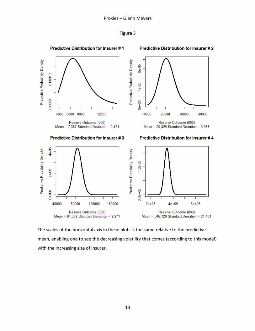
Figure 3 shows the plots of the predictive distributions and shows some summary

statistics.

2 The FFT of an aggregate loss distribution with a negative binomial claim count distribution is given by the probability generating function of the negative binomial distribution applied to the FFT of the claim severity distribution. See Klugman et. al. [2] for details.

Lagq

Lagq

Lagq

Lagq

Lagq


13

Figure 3

The scales of the horizontal axis in these plots is the same relative to the predictive

mean, enabling one to see the decreasing volatility that comes (according to this model)

with the increasing size of insurer.


14

6. Constructing the Scenarios

The scenarios used in this paper were constructed by examining the Schedule P paid

triangles for 50 large insurers. For each insurer I did the following:

1. Obtained estimates of the {ELRAY} and {DevLag} parameters by maximum likelihood

for each insurer using a generic numerical maximizing program.

2. Formed a “prior distribution” centered on the maximum likelihood estimate. Then,

using the Gibbs sampler (See Meyers [5]) I generated 100 additional {ELRAY} and

{DevLag} parameter sets. This generated a richer set of scenarios that could

conceivably represent the collection of the 50 insurers.

3. Randomly shuffled the {ELRAY} parameter set by Gibbs sample. I did the same,

independently, for the {DevLag} parameter set. I then bound them together to form

a set of 5,000 scenarios.

4. The scenarios generated above contained some obvious outliers. So I then capped

each of the ELRAY and DevLag parameters at the 1st and 99th percentiles for their

respective accident year and settlement lags.

This procedure was fairly time consuming. It took over a week to do this for all fifty

insurers. But once it is done, one can calculate the predictive distributions for any

insurer in a matter of minutes.

This procedure is meant to be purely illustrative. The general idea is to come up with a

rich set of scenarios that represents the range of reasonable outcomes. A jurisdiction

lacking the massive data that is reported to American regulators can rely on its best

judgment to select the scenarios.


15

7. Conclusion

The purpose of this paper is to illustrate a method an insurer with insufficient data or

little actuarial expertise, could use to derive a predictive distribution of its outstanding

loss liabilities. It is a mechanical procedure that involves plugging the available data into

a computer program that generates a predictive distribution of outcomes.

The appendix contains a program written in the R Programming Language and sample

data sets will be provided so that one can try running the program.

As one should intuitively expect, the predictive distributions can be relatively wide for

small insurers with little data but they narrow as the insurer becomes large and has

ample data.

The assumptions made in using this procedure are that are that the distribution of

losses is described by the collective risk model with an assumed claim severity

distribution and that some of the scenarios represent the possible {ELRAY} and {DevLag}

parameters.


16

References

1. CEIOPS – Groupe Consultatif Coordination Group on Proxies, “Draft Interim report including testing proposals for proxies under QIS 4, ” page 23, November 2007.

2. Klugman, Stuart A., Panjer, Harry A. and Willmot, Gordon E., Loss Models: From Data to Decisions, Second Edition, John Wiley and Sons, 2004.

3. Meyers, Glenn G., "The Common Shock Model for Correlated Insurance Losses,"

Variance 1:1, 2007, pp. 40-52. http://www.variancejournal.org/issues/01-01/040.pdf

4. Meyers, Glenn G., "Estimating Predictive Distributions for Loss Reserve Models," Variance 1:2, 2007, pp. 248-272.

http://www.variancejournal.org/issues/01-02/248.pdf

5. Meyers, Glenn G., ”Stochastic Loss Reserving with the Collective Risk Model,” Casualty Actuarial Society E-Forum 2008: Fall pp. 240-271. http://www.casact.org/pubs/forum/08fforum/11Meyers.pdf

6. Mildenhall, Stephen J., “Correlations and Aggregate Loss Distributions with an Emphasis on the Iman-Conover Method.” Casualty Actuarial Society Forum 2006: Winter pp. 103-204. http://www.casact.org/pubs/forum/06wforum/06w107.pdf



http://www.casact.org/pubs/forum/08fforum/11Meyers.pdf

http://www.casact.org/pubs/forum/06wforum/06w107.pdf


17

Appendix – Code for Calculating the Predictive Distribution

This appendix contains the code that produced Figures 1-3. It is written in the R

programming language. It reads three files that are electronically available with this

paper.

1. Capped and Shuffled Prior.csv – this file contains the 5,000 prior scenarios.

2. Severity Pareto.csv – this file contains the parameters of the Pareto distributions

in Section 2 of this paper.

3. Rectangle Proxies.csv – This file contains the data for the four insurers’ loss

triangles in Exhibit 1.

R code

# Input

comp=c(1,2,3,4)

pred.ay=c(2,rep(3,2),rep(4,3),rep(5,4),rep(6,5),rep(7,6),rep(8,7),rep(9,8),

rep(10,9)) #accident years in prediction

pred.lag=c(10,9:10,8:10,7:10,6:10,5:10,4:10,3:10,2:10) #development lags

#

######################### Begin Subprograms##############################

#

# estimate the step size for discrete loss distribution

#

estimate.h<-function(premium,fftn,limit.divisors){

h<-min(10*premium/2^fftn,max(limit.divisors)-1)

h<-min(subset(limit.divisors,limit.divisors>h))

return(h)

}

#

# Pareto limited average severity

#

pareto.las<-function(x,theta,alpha){

las<- ifelse(alpha==1,-theta*log(theta/(x+theta)),

theta/(alpha-1)*(1-(theta/(x+theta))^(alpha-1)))

return(las)

}

#

# discretized Pareto severity distribution

#

discrete.pareto<-function(limit,theta,alpha,h,fftn){

dpar<-rep(0,2^fftn)

m<-ceiling(limit/h)

x<-h*0:m

las<-rep(0,m+1)

for (i in 2:(m+1)) {

las[i]<-pareto.las(x[i],theta,alpha)

} #end i loop

dpar[1]<-1-las[2]/h

dpar[2:m]<-(2*las[2:m]-las[1:(m-1)]-las[3:(m+1)])/h

dpar[m+1]<-1-sum(dpar[1:m])

return(dpar)

} # end discrete.pareto function


18

#

# total reserve predictive distribution

#

totres.predictive.dist=function(eloss,ay,lag,posterior,esev,phiz){

npost=length(posterior)

phix=complex(2^fftn,0,0)

for (i in 1:npost){

phixp=complex(2^fftn,1,0)

for (j in unique(ay)){

dpp=rep(0,2^fftn)

lamp=0

ayp=(ay==j)

for (k in 1:length(lag[ayp])) {

kmin=lag[ayp][k]

lam=eloss[i,ayp][k]/esev[kmin]

lamp=lamp+lam

dpp<-dpp+dp[,kmin]*lam

} # end k loop

dpp<-dpp/lamp

phixp<-phixp*(1-myc*lamp*(fft(dpp)-1))^(-1/myc)

} # end j loop

phix=phix+posterior[i]*phixp

} # end i loop

pred=round(Re(fft(phix,inverse=TRUE)),12)/2^fftn

return(pred)

} #end totres predictive density

#

# likelihood for use in gibbs using overdispersed nb approximation

#

ccod.llike1=function(dev,elr){

eloss=rdata$premium*dev[rdata$dev]*elr[rdata$ay]

lam=outer(eloss/esev[rdata$dev],chi)

siz=lam/scv2

n1=round(rdata$loss/esev[rdata$dev])

llike1=dnbinom(n1,mu=lam,size=siz,log=T)

llike=sum(log(exp(rowsum(llike1,rdata$ay))%*%chiwt))

return(llike)

} # end ccod.llike1

#

# begin main program ##########################################################

#

h.step=rep(0,length(comp))

plot.range=matrix(0,length(comp),2)

myc=.01

chi=c(1-sqrt(3*myc),1,1+sqrt(3*myc))

chiwt=c(1/6,2/3,1/6)

# get prior distribution parameters

a=read.csv("Shuffled and Capped Prior.csv")

npriors=dim(a)[1]

elr.path=a[,2:11]

dev.path=a[,12:21]

#

# get loss data

#

r=read.csv("Rectangle Proxies.csv")

#

# get severity distributions and their ffts

#

fftn=14

limit.divisors=c(5,10,20,25,40,50,100,125,200,250,500,1000)

limit=1000

sevdist=read.csv("Severity Pareto.csv")

attach(sevdist)

pred=matrix(0,2^fftn,length(comp))

posterior=matrix(0,npriors,length(comp))

o=matrix(NA,npriors,length(comp))

mean.outcome=rep(0,length(comp))

sd.outcome=rep(0,length(comp))


19

#

# calculate predictive distributions and percentile of

# the sum of test diagonol losses for each insurer

#

windows(record=T)

for (i in 1:length(comp)){

#get reported data

rdata=subset(r,r$insurer_num==comp[i])

scv2=(elsm[rdata$dev]-esev[rdata$dev]^2)/esev[rdata$dev]^2

#get posterior probabilities for dev and elr parameters

lpost=rep(0,npriors)

for (n in 1:npriors){

elr=as.vector(elr.path[n,],mode="numeric")

dev=as.vector(dev.path[n,],mode="numeric")

lpost[n]=ccod.llike1(dev,elr)

}

posterior1=exp(lpost)

posterior1=posterior1/sum(posterior1)

o[,i]=order(-posterior1)

posterior[,i]=posterior1[o[,i]]

npost=max(sum(cumsum(posterior1[o[,i]])<.999),1)

#save time to calculate predictive distribution

posterior2=posterior1[o[,i]][1:npost]/sum(posterior1[o[,i]][1:npost])

pred.eloss=matrix(0,npost,length(pred.ay))

for (j in 1:length(pred.ay)){

for (n in 1:npost){

elr=as.vector(elr.path[o[,i],][n,],mode="numeric")

dev=as.vector(dev.path[o[,i],][n,],mode="numeric")

pred.eloss[n,j]=rdata$premium[pred.ay[j]]*elr[pred.ay[j]]*dev[pred.lag[j]]

}

}

#get the predictive distribution for the sum of losses in the test diagonal

h.step[i]=estimate.h(max(rowSums(pred.eloss)),fftn,limit.divisors)

phiz<-matrix(0,2^fftn,10)

dp<-matrix(0,2^fftn,10)

for (k in unique(pred.lag)){

dp[,k]<-discrete.pareto(limit,theta[k],alpha[k],h.step[i],fftn)

phiz[,k]<-fft(dp[,k])

} #end k loop

pred[,i]=totres.predictive.dist(pred.eloss,pred.ay,pred.lag,posterior2,esev,phiz)

#

# plot of elr paths

#

plot(1:10,elr.path[1,],ylim=range(0,elr.path),

main=paste("ELR Paths for Insurer #",comp[i]),

xlab="Accident Year",ylab="% Loss Paid",type="n")

for (j in 1:500){

par(new=T)

plot(1:10,elr.path[j,],ylim=range(0,elr.path),main="",

xlab="",ylab="",col="grey",type="l")

plotpost=cumsum(posterior[,i])<.995

}

for (j in 1:sum(plotpost)){

max.post=max(posterior[,i])

min.post=min(posterior[,i])

post.width=1+4*(posterior[j,i]-min.post)/(max.post-min.post)

par(new=T)

plot(1:10,elr.path[o[,i],][j,],ylim=range(0,elr.path),main="",

xlab="",ylab="",col="black",type="l",lwd=post.width)

}

legend("topleft",legend=c("Posterior","Prior"),

col=c("black","grey"),lwd=c(3,3))


20

#

# plot of development paths

#

plot(1:10,dev.path[1,],ylim=range(0,dev.path),

main=paste("Development Paths for Insurer #",comp[i]),

xlab="Settlement Lag",ylab="% Loss Paid",type="n")

for (j in 1:500){

par(new=T)

plot(1:10,dev.path[j,],ylim=range(0,dev.path),main="",

xlab="",ylab="",col="grey",type="l")

}

plotpost=cumsum(posterior[,i])<.995

for (j in 1:sum(plotpost)){

max.post=max(posterior[,i])

min.post=min(posterior[,i])

post.width=1+4*(posterior[j,i]-min.post)/(max.post-min.post)

par(new=T)

plot(1:10,dev.path[o[,i],][j,],ylim=range(0,dev.path),main="",

xlab="",ylab="",col="black",type="l",lwd=post.width)

}

legend("topright",legend=c("Posterior","Prior"),

col=c("black","grey"),lwd=c(3,3))

#

# plot density of outcomes

#

x=h.step[i]*(0:(2^fftn-1))

mean.outcome[i]=sum(x*pred[,i])

sd.outcome[i]=sqrt(sum(x*x*pred[,i])-mean.outcome[i]^2)

pred.range=(x>.5*mean.outcome[i])&(x<2*mean.outcome[i])

predb=pred[pred.range,i]

plot(x[pred.range],predb/h.step[i],type="l",col="black",lwd=3,

ylim=c(0,max(predb/h.step[i])),

xlim=range(x[pred.range]),

main=paste("Predictive Distribution for Insurer #",comp[i]),

xlab="Reserve Outcome (000)",ylab="Predictive Probability Density",

sub=paste("Mean =",format(round(mean.outcome[i]),big.mark=","),

"Standard Deviation =",format(round(sd.outcome[i]),big.mark=",")))

}

proxies - international actuarial association · proxies – glenn meyers 3 is equally likely, one...

Documents