psim: a computational platform for metabolic p systems€¦ · · 2015-07-29psim: a computational...

Psim: A Computational Platform for Metabolic PSystems

Luca Bianco

Cranfield UniversityCranfield HealthSilsoe, Bedfordshire, MK45 4DT, UKE-mail: [email protected]

Summary. Although born as unconventional models of computation, P systems can beconveniently adopted as modelling frameworks for biological systems simulations. Thischoice brings with it the advantage of producing easier to be devised and understoodmodels than with other formalisms. Nevertheless the employment of P systems for mod-elling purposes demands for biologically meaningful evolution strategies as well as forcomplete computational tools to run simulations on. In previous papers an evolutionstrategy known as metabolic algorithm has been presented, here a simulation tool calledPsim (current version 2.4) is discussed and a case study of its application is given as well.

1 Introduction

Membranes play a prominent role in living cells [1, 20]. In fact, membranes notonly act as a separation barrier indispensable to create different environmentswithin cells boundaries, but they can also physically constitute a kind of “workingboard” whereby enzymes can activate and perform their duties on substrates.Other examples of the crucial role of membranes within cells are their ability toperform selective uptakes and expulsion of chemicals as well as their being theinterface of the cell with the surrounding environment allowing communicationwith neighboring cells.

P systems originate from the recognition of this important role of membranesand, by abstracting from the functioning and structure of living cells, they providea novel computation model rooted in the context of formal language theory [33, 35].

P systems investigations are nowadays focused on several research lines thatmake the field “a fast Emerging Research Front” in computer science (as stated bythe Institute for Scientific Information). In particular, theoretical investigations onthe power of the computational model have been carried on and important resultshave been achieved so far in order to characterize the computational power of manyelements of P systems (such as objects and membranes) and, from a complexityviewpoint, P systems have been employed as well in the solution of NP hard

2 L. Bianco

problems. For a constant up to date bibliography of P systems we refer the readerto [39].

Parallel to these lines some more practical investigations are under way too.These studies exploit the resemblance of P systems to biological membranes inorder to develop computational models of interesting biological systems. P sys-tems seem to be particularly suitable to model biological systems, due to theirdirect correspondence of many elements (namely membranes, objects-chemicalsand rules-reactions), even in their basic formulation, with real biological entitiesbuilding the system to be modelled. Moreover, many extensions have been pro-posed to the standard formulation of P systems, such as some biologically relevantcommunication mechanisms [28, 36, 11], energy account [37] and active membranes[34] among others, which show the flexibility of the model. In this way, discretemathematical tools can be used to represent interesting biological realities to beinvestigated. A further step is that of simulating all systems described in this wayto get more information about their internal regulatory mechanisms and deeperinsights into their underlying elements.

Although born as a non-conventional model of computation inspired by nature,P systems can therefore be employed as a simulation framework in which to em-bed the in silico simulation of interesting biological systems. The strength of thischoice is, as said, the advantage that P systems share with biological systems manyof their features and this leads to easy-to-devise and easy-to-understand descrip-tions of the studied realities. In fact, the membrane construct in P systems hasa direct counterpart into biological membranes: objects correspond to all chemi-cals, proteins and macromolecules swimming in the aqueous solution within thecell and, eventually, rewriting rules represent biochemical reactions taking placein the controlled cellular environment. Other formalisms have been employed asmodelling and simulation frameworks too, such as Π calculus [29], Petri nets [38]and Ambient calculus [10], but in their case the very same notions of membranes,chemicals and reactions need to be reinterpreted and immersed in the particularrepresentation formalism in a less immediate way.

Nevertheless, the employment of P systems as a modelling framework for bio-logical systems posed, from a purely computational viewpoint, some new challengesto cope with, such as the identification of suitable, biologically meaningful, strate-gies for system evolution and the development of new automatic tools to describe,simulate and analyze the investigated system.

In previous works a novel strategy for systems evolution, called metabolic algo-rithm has been introduced [6, 27, 8], an hybrid (deterministic-stochastic) variant ofwhich has been proposed as well [5]. Other strategies of evolution are known, suchas Dynamical Probabilistic P systems [32, 31] and Multi-compartmental Gillespie’salgorithm [30, 2].

Here we will focus on the metabolic algorithm in its deterministic version whichhas been confronted with the dynamics of several systems (a collection of casestudies can also be found in [4]). Some examples of investigated systems by meansof the metabolic algorithm are the Belousov-Zhabotinsky reaction (in the Brus-

Psim: A Computational Platform for Metabolic P Systems 3

selator formulation) [6, 8], the Lotka-Volterra dynamics [6, 27, 7, 14], the SIR(Susceptible-Infected-Recovered) epidemic [6], the leukocyte selective recruitmentin the immune response [16, 6], the Protein Kinase C activation [8], circadianrhythms [12] and mitotic cycles in early amphibian embryos [26]. In order to copewith the demand of computational tools to simulate the dynamics of P systems,we developed a first simulator called Psim [6], which has now been extended withseveral new features as will be explained later on. The new version of the simulatoris freely available for download at [15].

The remaining of the discussion will firstly introduce (section 2) some theoret-ical aspects of the simulation framework we developed and some recent advanceswill be mentioned too. Section 3 will then be devoted to the newer version of thesimulator itself and a practical case study will be given as well in such a way toshow to the reader how to set up a simulation with the interface of Psim.

2 MP systems

MP systems (Metabolic P systems) [21, 26, 24, 23] are a special class of P systems[33, 35], introduced for expressing the dynamics of metabolic (or, more gener-ally speaking, biological) systems. Their dynamics is computed by means of adeterministic algorithm called metabolic algorithm which transforms populationsof objects according to a mass partition principle, based on suitable generalizationsof chemical laws.

A definition of MP systems follows, as given in [4].

Definition 1 (MP system). An MP system of level n − 1 (i.e., with n ∈ Nmembranes) is a construct:

Π = (T, µ,Q, R, F, q0)

in which:

• T is a finite set of symbols (or objects) called the alphabet;• µ is the hierarchical membrane structure, constituted by n membranes, labeled

uniquely from 0 to n − 1, or equivalently, associated in a one-to-one mannerto labels from a set L of n− 1 distinct labels;

• Q is the set of the possible states reachable by the MP system. Each elementq ∈ Q is a function q : T × L −→ R, from couples objects-membranes to realvalues. A value q(X, l), with X ∈ T and l ∈ L gives the amount of objectsX inside a membrane labeled l, with respect to a conventional unit measure(grams, moles, individuals, ...);

• R is the finite set of rewriting rules. Each r ∈ R is specified according to theboundary notation [3]. In other words, each rule r has the form αr −→ βr,where αr, βr are strings defined over the alphabet T enhanced with indexedparenthesis representing membranes. As an example, an hypothetical rule canhave the form: α[1β −→ γ[1δ, with α, β, γ, δ ∈ T ∗, meaning that α and β are

4 L. Bianco

respectively changed in γ and δ, where all objects within α and δ are outsidemembrane labeled 1, whereas elements of β and γ are placed inside membrane1;

• F is the set of reaction maps, each fr ∈ F is a function uniquely associated toa rule r ∈ R, defined as fr : Q −→ R and, given a certain state q, it producesfr(q) that is a real number specifying the strength of rule r in acquiring objects;

• q0 ∈ Q is the initial state of the system. It specifies the initial amount of allthe species throughout the various compartments of the system.

Since encodings like [9] show that the membrane structure can be flattened byaugmenting the alphabet size, the definition of the membrane structure µ is notvery important in this context and the choice to employ 0-level MP systems inthe remaining of the discussion is not limiting from a theoretical point of view.Moreover, dealing with 0-level MP systems ends up in a easier discussion, in factall states q ∈ Q do not need the specification of a membrane label and in this waythey have the simpler form: q : T −→ R. For this reason, in the following wheneverthe term MP system will be used, the more correct term 0-level MP system hasto be implicitly assumed.

The dynamics of MP systems has been calculated, starting from the initial stateq0 by means of an evolution strategy called metabolic algorithm [6, 27, 8], whichis substantially different from the well known non-deterministic and maximallyparallel paradigm followed by standard P systems. More precisely, the perspectiveof MP systems is to model systems at a population level rather than at an objectslevel. In this way, nothing can be precisely said about individuals but the investi-gation is focused on the macroscopic dynamics which assumes a deterministic flowin spite of individual behaviors.

2.1 The metabolic algorithm: hints

Without entering into many details (which can be found anyway in [6, 27, 8, 25]),the metabolic algorithm is a deterministic strategy for MP systems evolution basedon mass partition among rules of all elements in the alphabet T .

In very general terms, the metabolic algorithm can be summarized in the fol-lowing main points [26]:

• Reactants are distributed among all the rules, as the system evolves, accordingto a “competition” strategy.

• If some rules compete for the same reactant, then each of them obtains aportion of the available substance that is proportional to its reaction strength(reactivity) in that state.

• The reactivity of a rule in a certain state measures the capability of the ruleto acquire its reactants. It is calculated by the evaluation of the reaction mapcorresponding to the rule due and it depends on the state of the system, that isdefined as the concentration and localization of all substances in the consideredinstant.


• The evolution strategy determines the reaction unit of all rules, that is, theunitary amount of substance which is dealt by the rule. The stoichiometry isused then to obtain the consumed and/or produced amount of substances foreach rule.

An example may be useful to clarify the concepts yet introduced. Let us supposethat in a given instant, four rules, namely r1, r2, r3 and r4 ∈ R, need molecules ofa species A (with A belonging to the alphabet T ) as reactant (see Figure 1), thena partition strategy for A is necessary.

A

rr

rr 2

1

5

4

Fig. 1. Competition for object A between rules r1, r2, r4 and r5.

A real number called reactivity represents the strength of the rule (i.e. therule’s capability of obtaining matter to work on), given by the value assumed bya function uniquely associated to the rule called reaction map, in the consideredstate. For example, with respect to Figure 1, if we denote with a, b and c theconcentrations of species A, B,C respectively (in a state q not specified for thesake of simplicity), then the reactivities of rules r1, r2, r4 and r5, which ask for Amolecules, can be:

f1 = 200 · a, f2 = 0.5 · a1.25 · b−1, f4 = a1.25 · (b + c)−1 and f5 = 10

where the choice of reaction maps fi, i = {1, 2, 4, 5} is completely arbitrary inthis example.

We define the quantity

KA,q =∑

i=1,2,4,5

fi(q)

as the total pressure on A in the state q (the intuitive idea is that all reaction mapsof rules competing for a certain species give the force that pushes that species toreact).

Then, for each of the competing rules rj we consider the partial pressure (orweight) of rj on type A as

6 L. Bianco

wA,q(rj) =fj(q)KA,q

(again the idea behind this is that the strongest the force pushing an elementto follow a particular reaction channel, compared to other reaction channels, themore matter will follow that path).

Note that, in general, the quantity KX,q is defined for each couple (X, q) whereX ∈ T and q is a possible state of the system, moreover a weight wX,q(r) has tobe calculated for each triple (X, q, r) where X and q are respectively, as before, anelement of the biological alphabet and a state of the system, while r ∈ R is a rulein which the element X appears as a reactant (i.e., according to the terminologyadopted above, X ∈ αr).

Getting back to the example discussed above, it should be easy to see that thepartial pressure of r1 on A is

wA,q(r1) =200a

200a + 0.5a1.25b−1 + a1.25(b + c)−1 + 10

while the same pressure due to r2 results to be equal to

wA,q(r2) =0.5a1.25b−1

200a + 0.5a1.25b−1 + a1.25(b + c)−1 + 10

and the other weights can be calculated analogously. The weights calculated so fardetermine the partition factors of the amount of species A, available in the stateq, among the rules which need objects A as reactants.

Now to calculate the reaction unit of a particular rule (i.e. the amount ofreactant that can be dealt by the rule) we simply need to multiply the partialpressure of the rule on the reactant by the real amount of reactant present intothe system at the considered state. For example, the reaction unit of rule r1 (orequivalently, the amount of A that that can be assigned to rule r1) turns out tobe wA,q(r1) · a = 0.5a2.25b−1

200a+0.5a1.25b−1+a1.25(b+c)−1+10 .In this way, if r1 is a rule of the form A → X, no matter what element is

represented by X ∈ T , then the amount of A associated to r1 is exactly u1 =wA,q(r1) · a and the effect of r1’s application is the loss of u1 units of A and theacquisition of the same number of units of X.

In the case of cooperative rules (i.e. rules with more than just one reactant)things are a little bit more complicated since we need to take into account thereal availability of all reactants taking part to the reaction. That is, for eachX belonging to the reactants of a certain rule r we need firstly to compute thequantities wX,q(r) ·x and, since we have to respect species availability, the reactionunit associated to the rule is then computed as the minimum of those quantities.If we suppose that a rule r1 has the form AAB → X, then the reaction unit

u1 = min(12wA,q(r1) · a , wB,q(r1) · b)


where the term 12 in the first element of the minimum is due to the fact that A

appears twice in the stoichiometry of the rule.In general terms, the metabolic algorithm is an effective procedure for calcu-

lating in each state of the system a reaction unit ui for all rules ri ∈ R by using apartition strategy that employs particular functions fi associated in a 1-1 mannerto rules. After this calculation, the evolution of the system can be obtained in astraightforward way by consuming and producing species in a quantity given byrules’ reaction units and by following the stoichiometry of the system.

Assuming an ordering on objects and on rules, let us denote with M the m×nstoichiometric matrix associated to an MP system having m symbols and n rules(in which the ci,j element of M denotes the gain or the loss of the ith object dueto rule j1) and with Uq the [u1 · · ·un]T vector of the reaction units in a state ofthe system q, calculated as mentioned above.

Then, as pointed out in [25] the transition from one state q to the following oneis done by means of the delta operator (∆x(q)) which is a m-sized vector givingthe variation of each species in the transition from state q to the next state q′. Inparticular

∆x(q) = M × Uq

stating that the delta operator can be obtained as the product of the stoichiometricmatrix M by the reaction units vector of state q, Uq.

Since each row i of ∆x(q) gives the variation on the ith object, then if we thinkof a state q as a vector containing the concentration of all the m species at thecorresponding instant, then the next state can easily be calculated as

q′ = q + ∆x(q) = q + M × Uq.

Just to exemplify the last concepts discussed, we can think about an alphabetT = {A,B, C} and focus on a rule set comprising the following four rewritingrules:

r1 : A B −→ Cr2 : B B −→ Ar3 : C −→ Ar4 : C −→ B

then, assuming the lexicographic order on elements of the alphabet, we can obtainthe following stoichiometric matrix:

M =

−1 1 1 0−1 −2 0 1

1 0 −1 −1

in which, the first row corresponds to the object A and states that we lose oneconventional unit of A due to rule r1, we get one A both from rule r2 and r3 andfinally r4 does not affect A concentration at all.1 It is the difference between the number of occurrences of the ith symbol among prod-

ucts and among reactants of jth rule.

8 L. Bianco

Then, let us suppose to be in a state q, described by the vector of concentrationsq = [10 32 20]T (i.e. we have 10 units of A, 32 of B and 20 of C) and that thecorresponding reaction units vector Uq = [7 12 5 9]T (i.e. reaction r1 moves 7 massunits, r2 12, r3 5 and finally r4 9). In this way it is possible to calculate the nextstate q′ which turns out to be described by the following vector:

q′ = q + M × Uq =

103220

+

−1 1 1 0−1 −2 0 1

1 0 −1 −1

×

71259

=

201013

describing the amount of all species at that particular instant.In previous papers [26] a convenient and intuitive formalism for representing

MP systems called MP graphs has been proposed. In particular, MP graphs arebipartite graphs describing both the stoichiometry (i.e. the shape of the rules) andthe regulative part of MP systems that need to be effectively calculated in order toobtain the dynamics of the system (i.e. the reaction maps). According to what saidabove, MP graphs represent all the information needed to simulate MP systemsby means of the metabolic algorithm. An example of MP graphs, as produced bythe simulator we developed, will be shown later on.

2.2 Generalizing the metabolic algorithm

According to the formulation of the dynamics given in the previous section, themetabolic algorithm is a strategy that given a particular state q provides thesystem with the corresponding reaction units vector Uq which is used to calculatethe transition to the state q + 1. As discussed in [25], other strategies can beconsidered whose aim is to produce a reasonable mass partition among all rules ofan MP system, or in other words that give a different Uq for each state q of thesystem.

This view leads to the definition of several metabolic algorithms instead of asingle one and the definition of MP systems can be generalized accordingly.

Based on the definition given in [22], Definition 1 can be easily generalized, invery general terms, in the following way:

Definition 2 (Generalized MP systems). A 0-level (generalized) MP systemis a 6-tuple:

Π = (T, Q, R, V, q0, φ)

in which:

• T is a finite set of symbols (or objects) called the alphabet;• V is a finite set of variables;• Q is the set of the possible states reachable by the MP system. Each element

q ∈ Q is a function q : T ∪ V −→ R;• R is the finite set of rewriting rules;


• q0 ∈ Q is the initial state of the system;• φ is the strategy of evolution, φ : Q −→ Rn with |R| = n.

Note that nothing is said about the cardinality of the set of variables V and theyare not necessarily associated in a one-one manner to rules of R. Moreover, thestrategy of evolution φ, given a state q has to be defined in such a way that itoutputs the n-tuple providing the reaction unit vector of the system, or followingthe terminology used above, φ(q) = Uq.

Complete freedom is left in the implementation of the strategy of evolution,whose only constraints are that given a state it has to provide the reaction unitvector corresponding to that state, which will be used to calculate the evolutionof the system by means of the matrix product recalled in the previous section.As will be mentioned in the following, the specification of a fully customizablestrategy of evolution will be one of the prominent features of the new version ofthe simulator Psim that has been implemented within the MNC Group of theUniversity of Verona.

3 Psim

Based on the theoretical framework expressed in previous sections, a simulatorcalled Psim (P systems simulator) has been developed to cope with the problemof calculating the dynamics of biological systems. An early version of Psim has beendeveloped previously [6], with which the newer version shares the same philosophy,though extending some of its concepts and enhancing the simulation environmentwith many features.

The present release of Psim (version 2.4) has been developed in response tothe need of an effective and easy to use tool to calculate the dynamics of MPsystems by means of the metabolic algorithm. Its implementation has moreoverfollowed some flexibility and extensibility principles which led to a tool that canbe easily extended and integrated with other tools. In this way Psim, thanks toits immediate setup (nothing needs actually to be done provided a Java virtualmachine is installed on the computer that is meant to run Psim) and to the easyuser interface, can be used by people without a strong background in program-ming and a deep knowledge in the field of computer science. On the other hand,the extendability provided, as we will see, by means of the plugins mechanism,allows people with stronger expertise in programming to build their own tools tocomplement and integrate the main core of Psim.

Some features of this tool, which is implemented by using the Java program-ming language, are listed below:

• friendly user interface which is born to be easy-to-use and to interact withpeople not necessarily having a strong computer science background. Its im-mediacy can be found in the input side, which can be specified by means ofa transposition of the concept of MP graphs into a point and click graphical

10 L. Bianco

interface. Moreover, the same simplicity principle holds for the output side aswell, which is basically constituted by a graph containing the temporal evolu-tion of all the species constituting the system (both on a temporal scale andon the phase plan space);

• plugins architecture: the interaction with the system can either be done man-ually or by means of some specifically designed plugins which, thanks to theplugins support offered by the simulation engine, can interact with the sim-ulation engine itself. More specifically, three different kinds of plugins can bedevised and implemented in Java as well. Input plugins can be used to im-plement various sources for the data to run the simulation on (let us thinkto some specific pathways databases like KEGG for instance); output pluginsconversely, can be used to observe and analyze in various ways the results ob-tained from a simulation and can therefore give some meaningful insights intothe simulated dynamics. Moreover, they can be used to export simulation datainto particular formats. Finally, experiment plugins can directly control andintimately interact with the simulation engine, by controlling the executionflow, checking some properties and changing some experimental conditions.This kind of plugins can be very useful in tasks like model optimizations andstability analysis;

• extreme flexibility. The simulation tool we propose is based on a simulationengine which is designed to accept the definition of new evolution strategiesfor the calculation of the systems dynamics. At the only price of the imple-mentation of some specific interfaces, the developer has the chance to definehis own simulation strategies and to design a customized library of metabolicalgorithms to calculate the systems evolution;

• models portability has been implemented by using the standard XML languageand some extensions towards the SBML language are being considered too;

• cross platform applicability, thanks to the choice of Java, Psim can be run onall platforms supporting the Java virtual machine architecture.

An aspect deserving a special emphasis here is the possibility offered by the simu-lation engine, to specify custom evolution strategies. Getting back to the definitionof generalized MP systems, the architecture of the simulator allows the specifica-tion of a fully customized φ function. A set of evolution strategies can be devisedby developing in Java a specific class implementing a particular interface providedby the main engine. Several different strategies can be handled simultaneously bythe simulator that gives the chance to decide which simulation strategy employ inthe simulation process. This gives the tool a very high level of flexibility and poweras well as the plugins mechanism does. Since plugins can interact with the simu-lation engine at a different levels, such as input, output but also at the simulationlevel too, they can be used for various reasons within the simulator and this againgives users plenty of ways to improve the system and to extend its functionalities.


3.1 A case study

In this section we show an application of the Psim computational tool for thesimulation of the well known mitotic oscillator as found in early amphibian embryos[18, 19, 26].

Mitotic oscillations are a mechanism exploited by nature to regulate the onsetof mitosis, that is the process of cell division aimed at producing two identicaldaughter cells from a single parent. More precisely, mitotic oscillations concernthe fluctuation in the activation state of a protein produced by cdc2 gene in fissionyeasts or by homolog genes in other eukaryotes. The model here considered focuseson the simplest form of this mechanism, as it is found in early amphibian embryos.Here, the progressive accumulation of the cyclin protein leads to the activation ofcdc2 kinase. This activation is achieved by a bound between cyclin and cdc2 kinaseforming a complex known as M-phase promoting factor (or MPF ). The complextriggers mitosis and degrades cyclin as well; the degradation of cyclin leads to theinactivation of the cdc2 kinase that brings the cell back to the initial conditionsin which a new division cycle can take place.

Goldbeter [18, 19] proposed a minimal structure for the mitotic oscillator inearly amphibian embryos in which the two main entities are cyclin and cdc2 ki-nase. According to this model, depicted in Figure 2, the signalling protein cyclinis produced at a constant rate vi and it triggers the activation (by means of adephosphorylation) of cdc2 kinase, passing from the inactive form labelled M+ tothe active one, denoted by M . This modification is reversible and the other wayround is performed by the action of another kinase (not taken into account in themodel) that brings M back to its inactive form M+. Moreover, active cdc2 kinase(M) elicits the activation of a protease X+ that, when in the active (phosphory-lated) form (X), is able to degrade the cyclin. This activation, as the previous one,is reversible as stated by the arrow connecting X to X+.

The set of differential equations devised by Goldbeter produces an oscillatorybehavior in the activation of the three elements M , C, X that repeatedly gothrough a state in which cells enter in a mitotic cycle (see Figure 3).

The goal of the case study showed here is to obtain a description and a sim-ulation of the very same model of mitotic oscillations by means of the simulatorPsim.

In general, there is no unique way to translate a differential equation system interms of a metabolic P system, therefore we choose to obtain it by the applicationof the MP-ODE transformation [13]. The resulting MP system is reported here:

Π = (T, µ,R, F, q0)

where:

• The alphabet: T = {A,C, X, X+,M, M+}• The membrane structure: µ = [0 ]0;

12 L. Bianco

Fig. 2. The mitotic oscillator model by A. Goldbeter, from [18].

Fig. 3. Dynamics of the mitotic oscillator from [18].

• The set of rules is R = {r1, r2, ..., r10}, where:r1 : A → A Cr2 : C → Xr3 : X → λr4 : C → λr5 : C → M Cr6 : M+ → λr7 : M → M+

r8 : X+ → X Mr9 : M → λr10 : X → X+

in which all symbols have the meaning described before (and A is a kind of wellto draw substance C out from). Moreover, for every symbol in the system, we


have introduced an inertia rule (i.e., a rule having the form Y → Y , for eachY ∈ T to model the inertia of the system), omitted in this set of rules.

• The set of reaction maps is F = {Fr1, F r2, ..., F r10}, where:Fr1 = k1

Fr2 = k2x

k3+c

Fr3 = k2c

k3+c

Fr4 = k3

Fr5 = k5m+

(k6+c)(k7+m+)

Fr6 = k5c

(k6+c)(k7+m+)

Fr7 = k81

(k9+m)

Fr8 = k10m

(k11+x+)

Fr9 = k10x+

(k11+x+)

Fr10 = k121

(k13+x)

• The initial state q0 of the single membrane system is defined by:q0(A) = 1.3;q0(C) = 0.01;q0(X) = 0.01;q0(X+) = 0.99;q0(M) = 0.01;q0(M+) = 0.99;

in which we deal with concentrations of species, rather than with objects, andin this way the initial amounts are real numbers;

where, for each element of T the reaction map of inertia rules is set to 1600.We start the modeling session by opening the Psim’s main interface showed in

Figure 4. This window allows the user to manage all the experiment’s stages. Inparticular the main possible choices involve:

1. modelling the system, setting substances, initial conditions, reaction maps andrules;

2. starting the simulation;3. displaying output charts.

The first step to consider while setting up a system’s simulation is the speci-fication of the corresponding MP graph. In what follows, some steps towards thecreation of an MP graph modelling the mitotic oscillator are presented.

After clicking on the New Experiment label of the File menu, a window likethe one depicted in the Figure 5 appears. This is the main window of the graphicalinterface allowing the user to input in a easy way the MP graph components bysimply dragging them from the upper toolbar to the bottom white panel. Thistask is performed by using the following toolbar icons:

• The blue circle: adds a new type node that stores the name of a substance, itsinitial number of molar units and its inertia value (as explained in previouspapers, inertias are a way to represent the fact that not all reactants need to

14 L. Bianco

Fig. 4. The Psim’s main interface

Fig. 5. Psim’s input interface

react at a certain instant, they are a sort of resistance opposed to species toperforming reactions).

• The black circle: adds a new metabolic reaction node that represents a reactionchannel between interacting substances and stores the name of a reaction rule.

• The red rectangle: adds a new reactivity node building the regulatory part ofMP graphs. In the simulator, reactivity nodes store the reactivity map functioncorresponding to the connected rule and, if necessary, a boolean guard functionfor the rule activation.


• The green triangles: add input gates and output gates nodes that identify ruleswhich respectively introduce new matter in the membrane or expel part of itfrom the system.

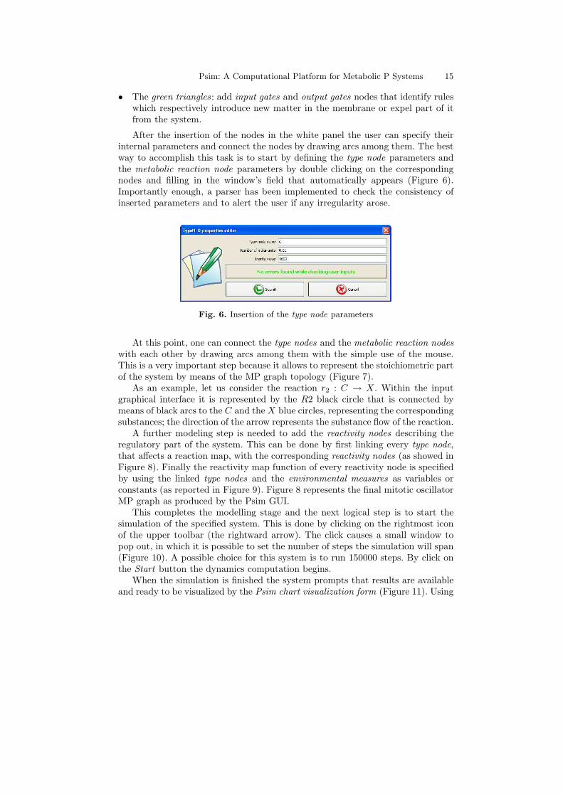
After the insertion of the nodes in the white panel the user can specify theirinternal parameters and connect the nodes by drawing arcs among them. The bestway to accomplish this task is to start by defining the type node parameters andthe metabolic reaction node parameters by double clicking on the correspondingnodes and filling in the window’s field that automatically appears (Figure 6).Importantly enough, a parser has been implemented to check the consistency ofinserted parameters and to alert the user if any irregularity arose.

Fig. 6. Insertion of the type node parameters

At this point, one can connect the type nodes and the metabolic reaction nodeswith each other by drawing arcs among them with the simple use of the mouse.This is a very important step because it allows to represent the stoichiometric partof the system by means of the MP graph topology (Figure 7).

As an example, let us consider the reaction r2 : C → X. Within the inputgraphical interface it is represented by the R2 black circle that is connected bymeans of black arcs to the C and the X blue circles, representing the correspondingsubstances; the direction of the arrow represents the substance flow of the reaction.

A further modeling step is needed to add the reactivity nodes describing theregulatory part of the system. This can be done by first linking every type node,that affects a reaction map, with the corresponding reactivity nodes (as showed inFigure 8). Finally the reactivity map function of every reactivity node is specifiedby using the linked type nodes and the environmental measures as variables orconstants (as reported in Figure 9). Figure 8 represents the final mitotic oscillatorMP graph as produced by the Psim GUI.

This completes the modelling stage and the next logical step is to start thesimulation of the specified system. This is done by clicking on the rightmost iconof the upper toolbar (the rightward arrow). The click causes a small window topop out, in which it is possible to set the number of steps the simulation will span(Figure 10). A possible choice for this system is to run 150000 steps. By click onthe Start button the dynamics computation begins.

When the simulation is finished the system prompts that results are availableand ready to be visualized by the Psim chart visualization form (Figure 11). Using

16 L. Bianco

Fig. 7. Adding type nodes, metabolic reaction nodes and drawing arches among them

Fig. 8. An MP graph that models the mitotic oscillator

Fig. 9. Reactivity node input parameter window


Fig. 10. Set the number of steps for the simulation to 150000

the bottom panel check boxes it is possible to decide elements to be displayed. Inthe considered case oscillations of cyclin C (red line), active cdc2 kinase M (blueline) and active protease M (green line) are displayed but the phase space plotcan be drawn as well.

Fig. 11. Oscillations of the mitotic systems as calculated by Psim.

We finally highlight an important mechanism of the Psim platform: pluginsextensibility. As already mentioned, plugins allow the user to enhance the mainPsim computing core with powerful functionalities for the data import, export,control and analysis. An example under development is the experiment plugin thatstores the experiment state (concentration of the substances and environmentalmeasures) every x steps, where x is a parameter set by the user before the com-putation starts. This plugin could save, for instance, an XML file for every state,allowing the user to export the experiment samples in an standard way.

A software developer generates the plugin code (basically some Java classes)relying on the Psim’s JavaDoc documentation obtainable at [15] which lists theexperiment plugin methods to be mandatorily implemented. Plugin classes are

18 L. Bianco

meant to be archived in a Jar file and placed in a proper plugins directory. Providedthis, at the following start up Psim will automatically find and load all the pluginscontained in the plugins directory. The user can find all available experiment pluginstatements in the main interface Experiment Plugin menu (Figure 4) in the formof a list. By clicking on the relative label its possible to activate the plugin thatwill be run at each step of the subsequent simulation and will save the state everyx steps chosen by the user filling in a plugin popup window.

The plugin just described yields a set of XML files but the same principles canbe extended also to the other kinds of plugins (input, output, engine plugins).

A particular mention is deserved by engine plugins that allow to implementnew simulation strategies which can be different from the metabolic algorithmdescribed above. This gives the simulation tool a very high flexibility as well asextendability as discussed previously.

4 Conclusion and further work

P systems can be useful frameworks to embed biological systems models in. Thisdemands for some modifications to the classical definition of P systems and par-ticularly a biologically meaningful evolution strategy is needed. In previous papersan essentially deterministic strategy, called metabolic algorithm, for the calcula-tion of biological systems dynamics has been provided as well as an extension ofthe classic model of P systems, known as MP systems, focused on the dynamics ofbio-systems. Moreover, all data needed for the simulation of MP systems dynamicscan be provided by means of a graphical formalism known as MP graphs.

The basics of MP systems have been briefly revisited in this paper and basedon them a simulation tool called Psim has been highlighted, together with a casestudy of a well known and previously investigated model of mitotic cycles in earlyamphibians. Psim v. 2.4 is the latest release of the MP systems simulator developedwithin the MNC Group of the University of Verona and it has very interestingfeatures such as the plugin mechanism and the meta-engine architecture which givethe tool an high level of extendability and personalization. In particular, pluginscan be useful to perform several tasks such as data import/export, control of thesimulation flow, output of dynamics obtained and analysis of the results amongothers. Moreover, the meta-engine architecture of the simulator allows users todefine their own evolution strategies by implementing some fixed interfaces of thesimulator.

In the future we plan to enrich the core of this simulation tool by implementinga series of plugins such as the one described above to have a snapshot of the state ofthe system in particular instants. Other plugins under investigation involve someautomatic procedures for parameter estimation given suitable observations of thereality to be modelled. Finally, we plan to employ this simulation tool for thecalculation of the dynamics of systems not already modelled and in this respectthe possibility to devise ad-hoc evolution strategies can be very important to tacklesome specific issues related with the particular reality to be modelled.


References

1. B. Alberts, A. Johnson, J. Lewis, M. Raff, K. Roberts, and P. Walter. Biology of theCell. Garland Science, New York, 4th edition, 2002.

2. F. Bernardini, M. Gheorghe, N. Krasnogor, R.C. Muniyandi, M.J. Perez-Jimenez,and F.J. Romero-Campero. On P Systems as a modelling tool for biological systems.In R. Freund, G. Lojka, M. Oswald, and Gh. Paun, editors, Pre-Proceedings of the 6thInternational Workshop on Membrane Computing (WMC6), pages 193–213, 2005.

3. F. Bernardini and V. Manca. Dynamical aspects of P systems. BioSystems, 70:85–93,2002.

4. L. Bianco. Membrane Models of Biological Systems. PhD thesis, Verona University,2007.

5. L. Bianco and F. Fontana. Towards a Hybrid Metabolic Algorithm. In H. J. Hooge-boom, G. Paun, and G. Rozenberg, editors, 7th International Workshop on Mem-brane Computing, WMC07 Leiden. Selected Papers, number 4361 in LNCS, pages183–196. Springer-Verlag, Berlin, 2006.

6. L. Bianco, F. Fontana, G. Franco, and V. Manca. P systems for biological dynamics.In G. Ciobanu, G. Paun, and M. J. Perez-Jimenez, editors, Applications of MembraneComputing. Springer, Berlin, 2006.

7. L. Bianco, F. Fontana, and V. Manca. Reaction-Driven Membrane Systems. InK. Chen L. Wang and Y.S. Ong, editors, Advances in Natural Computation, FirstInternational Conference, ICNC 2005 (part II), Proceedings of ”First InternationalConference in Natural Computation (ICNC 2005)”, pages 1155–1158. Springer, 2005.

8. L. Bianco, F. Fontana, and V. Manca. P systems with reation maps. InternationalJournal of Fondations of Computer Science, 16(1), 2006.

9. L. Bianco and V. Manca. Encoding-Decoding Transitional Systems for classes of PSystems. In Freund et al. [17], pages 135–144.

10. L. Cardelli and A. D. Gordon. Mobile Ambients. In M. Nivat, editor, Proceed-ings of the First international Conference on Foundations of Software Science andComputation Structure. LNCS 1378, Springer, 1998, pages 140–155.

11. M. Cavaliere. Evolution-Communication P Systems. In G. Paun, G. Rozenberg,A. Salomaa, and C. Zandron, editors, Membrane Computing: International Work-shop, WMC-CdeA 2002, Curtea de Arges,Romania, August 19-23, 2002. RevisedPapers., volume 2597 of Lecture Notes in Computer Science, pages 134–145, Curteade Arges, Romania, July 2003. Springer-Verlag, Berlin.

12. F. Fontana, L. Bianco, and V. Manca. P systems and the Modeling of BiochemicalOscillations. In Freund et al. [17], pages 199–208.

13. F. Fontana and V. Manca. Discrete Solution of Differential Equations by MetabolicP Systems. Submitted to TCS, 2006.

14. F. Fontana and V. Manca. Predator-prey Dynamics in P Systems Ruled by MetabolicAlgorithm. BioSystems, Accepted, 2006.

15. The Center for BioMedical Computing Web Site. Url: http://www.cbmc.it.16. G. Franco and V. Manca. A membrane system for the leukocyte selective recruit-

ment. In A. Alhazov, C. Martin-Vide, and G. Paun, editors, 4th Workshop on Mem-brane Computing, volume 2933 of Lecture Notes in Computer Science, pages 180–189.Springer-Verlag, 2004.

17. R. Freund, G. Paun, G. Rozenberg, and A. Salomaa, editors. Membrane Computing,6th International Workshop, WMC 2005, Vienna, Austria, July 18-21, 2005, RevisedSelected and Invited Papers, volume 3850 of Lecture Notes in Computer Science.Springer, 2006.

20 L. Bianco

18. A. Goldbeter. A Minimal Cascade Model for the Mitotic Oscillator Involving Cyclinand cdc2 Kinase. PNAS, 88(20):9107–9111, 1991.

19. A. Goldbeter. Biochemical Oscillations and Cellular Rhythms. The molecular basesof periodic and chaotic behaviour. Cambridge University Press, New York, 2004.

20. H. F. Lodish, A. Berk, P. Matsudaira, C. Kaiser, M. Krieger, M. Scott, L. Zipursky,and J. E. Darnell. Molecular Cell Biology. Scientific American Press, New York, 5thedition, 2004.

21. V. Manca. Topics and problems in metabolic p systems. In Proc. of the FourthBrainstorming Week on Membrane Computing (BWMC4), 2006.

22. V. Manca. Discrete Simulations of Biomolecular Dynamics. Submitted, 2007.23. V. Manca. Metabolic Dynamics by MP Systems. In InterLink ERCIM Workshop,

Eze, France, May 10-12, 2007.24. V. Manca. Metabolic P systems for Biochemical Dynamics. Progress in Natural

Sciences, Invited Paper, 2007.25. V. Manca. The Metabolic Algorithm for P Systems Principles and Applications.

Submitted, 2007.26. V. Manca and L. Bianco. Biological Networks in Metabolic P Systems. BioSystems,

Accepted, 2006.27. V. Manca, L. Bianco, and F. Fontana. Evolutions and oscillations of P systems:

Theoretical considerations and applications to biochemical phenomena. In G. Mauri,G. Paun, M. J. Perez-Jimenez, G. Rozenberg, and A. Salomaa, editors, MembraneComputing, International Workshop, WMC5, Milano, Italy, 2004, Selected Papers,number 3365 in LNCS, pages 63–84. Springer-Verlag, Berlin, 2005.

28. C. Martin-Vide, G. Paun, and G. Rozenberg. Membrane systems with carriers.Theoretical Computer Science, 270:779–796, 2002.

29. R. Milner. Communicating and Mobile Systems: The π Calculus. Cambridge Uni-versity Press, Cambridge, England, 1999.

30. M. J. Perez-Jimenez and F. J. Romero-Campero. P systems: a new computationalmodelling tool for systems biology. Transactions on Computational Systems BiologyVI, Lecture Notes in Bioinformatics, 4220, pages 176–197, 2006.

31. D. Pescini, D. Besozzi, and G. Mauri. Investigating local evolutions in dynamicalprobabilistic p systems. In In G. Ciobanu, Gh. Paun, Pre-Proc. of First InternationalWorkshop on Theory and Application of P Systems, Timisoara, Romania, September26-27, pages 83–90, 2005.

32. D. Pescini, D. Besozzi, G. Mauri, and C. Zandron. Dynamical probabilistic P systems.International Journal of Foundations of Computer Science, 17(1):183, 2006.

33. G. Paun. Computing with membranes. J. Comput. System Sci., 61(1):108–143, 2000.34. G. Paun. P Systems with Active Membranes: Attacking NP-Complete Problems.

Journal of Automata, Languages and Combinatorics, 1(6):75–90, 2001.35. G. Paun. Membrane Computing. An Introduction. Springer, Berlin, Germany, 2002.36. G. Paun and A. Paun. The power of communication: P systems with sym-

port/antiport. New Generation Computing, 20(3):295–306, 2002.37. G. Paun, Y. Suzuki, and H. Tanaka. P systems with energy accounting. Int. J. Com-

puter Math., 78(3):343–364, 2001.38. W. Reisig. Petri Nets, An Introduction. EATCS, Monographs on Theoretical Com-

puter Science. 1985.39. The P Systems Web Site. Url: http://psystems.disco.unimib.it.

psim: a computational platform for metabolic p systems€¦ · · 2015-07-29psim: a computational...

Documents