pso trained ann-based differential protection scheme...

ARTICLE IN PRESS

0925-2312/$ - se

doi:10.1016/j.ne

�CorrespondE-mail addr

Neurocomputing 71 (2008) 904–918

www.elsevier.com/locate/neucom

PSO trained ANN-based differential protection schemefor power transformers

M. Geethanjali�, S. Mary Raja Slochanal, R. Bhavani

Department of Electrical and Electronics Engineering, Thiagarajar College of Engineering, Madurai 625 015, Tamilnadu, India

Received 3 May 2006; received in revised form 11 October 2006; accepted 26 February 2007

Communicated by A. Zobaa

Available online 7 April 2007

Abstract

In this paper, a novel scheme is proposed which monitors and discriminates the different operating conditions (normal, magnetizing

inrush current, over excitation of the core, internal faults and CT saturation due to external faults) of power transformers. The Particle

Swarm Optimization (PSO) technique is used to train the multi-layered feed forward neural networks to discriminate the different

operating conditions. The proposed scheme has been realized through two different Artificial Neural Network (ANN) architectures. One

is used as an internal fault detector and the other one detects and discriminates the other operating conditions like normal, inrush, over

excitation, and CT saturation due to external faults. These two ANNs were trained using Back Propagation Neural Network Algorithm

(BPN) and PSO technique and the simulated results are compared. Simulations are performed for the practical power transformer

ratings obtained from Tamilnadu Electricity Board (TNEB), India. Comparing the simulated results of the above two cases, training the

neural network by PSO technique gives more accurate (in terms of sum square error) and also faster (in terms of number of iterations and

simulation time) results than BPN. The PSO trained ANN-based differential protection scheme provides faster, accurate, more secured

and dependable results for power transformers.

r 2007 Elsevier B.V. All rights reserved.

Keywords: Power transformer; Differential protection; Artificial Neural Network (ANN); Particle Swarm Optimization technique

1. Introduction

Power transformer is one of the most important classes ofhardware in the electric power system, and the transformerprotection is an essential part of the overall system protectionstrategy. The design of protective relay has to consider variousnonlinear effects, which may cause malfunction of the relayequipments. The most common method of transformerprotection utilizes the percentage differential relay as theprimary protection. Discrimination between an internal faultand other operating conditions such as magnetizing inrushcurrent, over excitation, CT saturation is recognized as achallenging power transformer protection problem.

Differential protection of transformers using harmonicrestraint to prevent tripping on magnetizing inrush and

e front matter r 2007 Elsevier B.V. All rights reserved.

ucom.2007.02.014

ing author.

ess: [email protected] (M. Geethanjali).

over excitation has been developed successfully for severaldecades [11,10]. The ratio of second and fifth harmonicstogether with the fundamental frequency component of thedifferential current has been widely used as a faultdiscriminate to distinguish the other operating conditionsof the transformers from internal faults. With the advent ofintroduction of various advancements in the powersystems, the detection of second or fifth harmonic aloneis not sufficient to do the discrimination. Moreover, thisconventional technique based on second harmonic restrainhas complexity in distinguishing among internal fault,inrush current, CT saturation and over excitation therebyaffecting transformer stability. Therefore, a method basedon the use of one of the primary phase voltage as thecontrol signal is proposed [3]. Later alternative improvedprotection techniques based on transient detection weredeveloped for accurate and efficient discrimination [9].In the recent past, numerical protection/digital protec-

tion was introduced to improve the protection schemes.

www.elsevier.com/locate/neucom

dx.doi.org/10.1016/j.neucom.2007.02.014

mailto:[email protected]

ARTICLE IN PRESS

Inputs

Interconnection

Hidden layer

Interconnection

Outputs

Fig. 1. Multi-Layered Feed Forward Neural Network (MLFFNN).

M. Geethanjali et al. / Neurocomputing 71 (2008) 904–918 905

As with classical static protection, new numerical protec-tion can also lead to unnecessary operation or operationfailures. This is because of the inability of protectionalgorithms to distinguish transient states from faults. Toovercome this difficulty, recently various artificial intelli-gent (AI) techniques are introduced to power systemprotection [9,5]. Among various AI techniques, theArtificial Neural Network (ANN) have become mostfrequently used modern data processing/decision makingalgorithm to solve numerous complex engineering pro-blems, because of their well known advantages likepossibility of learning from examples, generalizationability, parallel computation, nonlinear mapping nature,etc. Recently, the possible application of neural networksto achieve some protective relay functions is a matter ofresearch. ANN-based power transformer protection hasbeen done using Back Propagation Network (BPN) andRadial Basis Function Network (RBFN) by Moravej et al.[5–8]. In these cases, the differential relay using ANNshould recognize and discriminate all the possible condi-tions (such as normal, inrush, over excitation, internal faultCT saturation due to external faults). The discriminationprocess mainly depends on the harmonic components andback propagation is the most common technique used forsuch neural networks [4]. A neural network approach usingtwo different ANN architectures for fault discriminationbased on recognizing its wave shape and its harmonicspectrum, respectively, has been proposed [4]. But toobtain still more effective and fast discrimination, ParticleSwarm Optimization technique (PSO) technique has beenintroduced to train the ANN architecture. PSO algorithmis preferred because of its successful implementation tosolve many complex optimization problems in electricalengineering [1,2].

In this paper, the proposed scheme has been realizedthrough two different ANN architectures. One is used asan internal fault detector and the other one detects anddiscriminates the other operating conditions like normal,inrush, over excitation, and CT saturation due to externalfaults. The developed ANN architectures are trained byusing feed forward back propagation algorithm and PSOtechnique algorithm. The data for training and testingneural networks were developed using SIMULINK mod-eling (in MATLAB 6.5) of power transformers for theabove said different operating conditions for 20 differentpractical power transformers with different ratings ob-tained from Tamilnadu Electricity Board (TNEB), India[12]. The features of the simulated differential currentwaveforms were extracted using FFT block (Fast FourierTransform) in the simulink model and used as inputs to theANN architectures. The ANN architectures were trainedusing BPN (Back Propagation Neural Network Algorithm)and then using PSO technique. PSO algorithm is preferredbecause PSO has no evolution operators such as crossoverand mutation. Also, it is easy to implement and there arefew parameters to adjust. PSO has been successfullyapplied in many areas like function optimization, artificial

neural network training, fuzzy system control, and otherareas where genetic algorithm can be applied.

2. Overview of ANN

ANN is basically a simplified model of the biologicalneuron and uses an approach similar to human brain tomake decisions and to arrive at conclusions. It is composedof large number of highly interconnected processingelements (neurons) working in union to solve specificproblems. Neural network learns from experience. AnANN is configured for a specific application, such aspattern recognition or data classification, through alearning process. Learning involves adjustments of synapticconnections (i.e. weights) among the neurons. Everyneuron model consists of a processing element withsynaptic input connections and a single output. Theneuron can be defined as

yk ¼ fX

xjnwkj

� �, (1)

where x1, x2, y, xj are input signals, wk1, wk2, y, wkj aresynaptic weights of neuron k, f(.) is the activation functionand yk is the output signal of neuron.Of all the different types of neural networks used in the

recent past, the neural network, which is used mostprevalently in power system protection applications, isthe Multi-Layered Feed Forward Neural Network(MLFFNN) with back propagation training algorithmbecause of its simplicity and good generalization. Hence,MLFFNN is used for the proposed work.

2.1. Multi-Layered Feed Forward Neural Network

2.1.1. Architecture

The architecture of multi-layered feed forward neuralnetwork is shown in Fig. 1. It consists of one input layer,one output layer and hidden layer. It may have one ormore hidden layers. All layers are fully connected and ofthe feed forward type. The outputs are nonlinear functionof inputs, and are controlled by weights that are computed

ARTICLE IN PRESSM. Geethanjali et al. / Neurocomputing 71 (2008) 904–918906

during learning process. The used learning process issupervised type and the learning paradigm is the backpropagation. For the BP training process, a boundeddifferentiable activation function is required. The mostcommonly known function that is called the sigmoid hasbeen used. It is bounded between the minimum (0) andmaximum (1). Before a signal is passed to the next layer ofneurons, the summed output of each neuron is scaled bythis function.

2.1.2. Learning

The key to error propagation network learning is itsability to change its synaptic weights in response to errors.Fig. 2 shows the block diagram of this learning (i.e.) backpropagation (BP) algorithm.

2.1.3. BP algorithm

The MLFFNN is usually trained in a supervised mannerwith a highly popular algorithm known as error backpropagation algorithm. Information about errors is alsofiltered back through the system and is used to adjust theconnections between layers, thus improving the perfor-mance. The error BP process consists of two passes throughthe different layers of network, namely: forward pass andbackward pass. In the forward pass, an activation pattern isapplied to the sensory nodes of the network, and its effectpropagates through the network layer by layer. Finally, a setof outputs is produced as the actual response of thenetwork. The actual response of the network is subtractedfrom a desired response to produce error signal. This errorsignal is then propagated backward through the networkagainst the direction of the synaptic connections. Thesynaptic weights are adjusted so as to make the actualresponse of the network much closer to the desired response.

2.1.4. Steps in training BP network

1.
Select training pair from the training set and apply theinput vector to the input layer.
2.
Calculate the output of the network. 3. Calculate the error between the network output and the
desired output.
4. Adjust the weights of the network in a way that
minimizes the error.

Original system

EnvironmentTeacher Known

Input-output data

Learning of ANN

Target

Computed error

Actual

output

Inputs

Fig. 2. Block diagram of supervised learning.

5.
Repeat steps 1–4 for each vector in the training set untilthe error for the entire set is acceptably low.
Usually to minimize the sum of squares of the errors, theleast mean square method is used. In these algorithms,steps 1 and 2 constitute a forward pass and steps 3 and 4constitute a reverse pass.

3. Overview of PSO technique

PSO is an evolutionary computation technique devel-oped by Dr. Eberhart and Dr. Kennedy in 1995, inspiredby social behavior of bird flocking or fish schooling.Similar to genetic algorithms (GA), PSO is a population-based optimization tool. The system is initialized with apopulation of random solutions and searches for optima byupdating generations. However, unlike GA, PSO has noevolution operators such as crossover and mutation. InPSO, the potential solutions, called particles are ‘‘flown’’through the problem space by following the currentoptimum particles. Since there are only few parameters toadjust in PSO, it is easy to implement.

3.1. PSO algorithm

PSO simulates the behaviors of bird flocking. In PSO,each single solution is a ‘‘bird’’ in the search space. Here, itis called as ‘‘particle’’. All the particles have fitness values,which are evaluated by the fitness function to be optimized,and have velocities, which direct the flying of the particles.The particles are ‘‘flown’’ through the problem space byfollowing the current optimum particles. PSO is initializedwith a group of random particles (solutions) and thensearches for optima by updating generations. In each oneof the iterations, iteration, each particle is updated byfollowing two ‘‘best’’ values. The first one is the bestsolution (fitness) it has achieved so far. (The fitness value isalso stored.) This value is called pbest. Another ‘‘best’’value that is tracked by the particle swarm optimizer is thebest value, obtained so far by any particle in thepopulation. This best value is a global best and calledgbest. After finding the two best values, the particle updatesits velocity and positions with Eqs. (2) and (3):

V id ¼W � V id þ c1 � randð Þ � ðPid � X idÞ

þ c2 � randð Þ � ðPgd � X idÞ; ð2Þ

X id ¼ X id þ V id, (3)

where W is the inertia weight, Vid is the particle velocity,Xid is the current particle (solution), Pid and Pgd are pbestand gbest, rand ( ) is a random number between (0,1) andc1, c2 are learning factors.Particle’s velocities on each dimension are clamped to a

maximum velocity Vmax. If the sum of accelerations wouldcause the velocity on that dimension to exceed Vmax, whichis a parameter specified by the user then the velocity onthat dimension is limited to Vmax.

ARTICLE IN PRESSM. Geethanjali et al. / Neurocomputing 71 (2008) 904–918 907

3.2. PSO parameter control

There are two key steps when applying PSO tooptimization problems, namely the representation of thesolution and the fitness function. For example, if thesolution for f ðxÞ ¼ x2

1 þ x22 þ x2

3, is to be determined, thenthe particle can be set as (x1, x2, x3), and fitness function isf(x). Then the standard procedure to find the optimum isused. The searching is a repeat process, and the stopcriteria are that the maximum iteration number is reachedor the minimum error condition is satisfied. There are somany parameters need to be tuned in PSO.

3.2.1. Tuning of parameters

The typical ranges of number of particles are 20–40.Actually for most of the problems 10 particles is largeenough to get good results. For some difficult or specialproblems, 100 or even 200 particles shall be tried. Thedimensions of particles are determined by the problem tobe optimized. The ranges of particles for differentdimensions of particles can be specified. Velocity deter-mines the maximum change that each particle can takeduring each one of the iterations. Regarding learningfactors (c1 and c2), usually, c1 equals c2 and ranges from[0,4]. In most of the cases both c1 and c2 are equal to 2.However, other settings were also used in different papers.The stop condition also depends on the problem to beoptimized. Usually, it is determined by the maximumnumber of iterations the PSO execute and the minimumerror requirement.

3.2.2. Inertia weight (W)

Another factor, inertia weight, was developed to controlexploration and exploitation. The inclusion of an inertiaweight in the PSO algorithm eliminates the need for Vmax.The maximum velocity Vmax serves as a constraint tocontrol the global exploration ability of a particle swarm.A larger Vmax facilitates global exploration, while a smallerVmax encourages local exploitation. Eqs. (2) and (3)describe the velocity and position update equations withan inertia weight inclusion. The use of the inertia weighthas provided improved performance in a number of

Power

transformer

modeling

(simulink)

FFT

Input

data

Simulated differential

current signals Discrete

signals

Fig. 3. Block diagram of

applications. Suitable selection of the inertia weightprovides a balance between global and local explorationand exploitation, and results in lesser iterations on averageto find a sufficiently optimal solution.

4. Proposed scheme

This scheme presents an application of neural network indigital power transformer protection. Neural network ispreferred because of its self-learning and highly nonlinearmapping capability. This ANN-based scheme monitorsdifferent operating conditions of power transformers,detects the fault and issues a trip signal in the case offaults. This scheme has been realized through two differentANN architectures using feed forward back propagationalgorithm and PSO technique. The result demonstrates thecapabilities of internal fault detector (IFD) and conditionmonitor (CM) in terms of accuracy and speed with respectto detection of fault and pattern recognition of differentevents of power transformers.The basic block diagram of the proposed scheme is given

in Fig. 3.

4.1. Power transformer modeling

A suitable transformer model is required to characterizethe different operating conditions of power transformer. Atransformer model can be viewed as a functional approx-imator and it provides terminal behavior of powertransformer under various situations. Such a transformeris modeled using SIMULINK (in MATLAB 6.5). Thismodel allows simulation of faults and other disturbancesthat can lead to a false operation of the power systemprotection.Operating conditions considered:

�

the

normal,
� magnetizing inrush current (due to transformer energi-
zation),
� over excitation, � CT saturation (due to external fault), � internal fault.
ANN

Architecture for

Internal Fault

Detector (IFD)

ANN

Architecture for

Condition

Monitor (CM)

1000 (Normal)

1000 (Inrush)

0010 (Over

Excitation)

0010 (CT

Saturation)

1 (or) 0

proposed scheme.


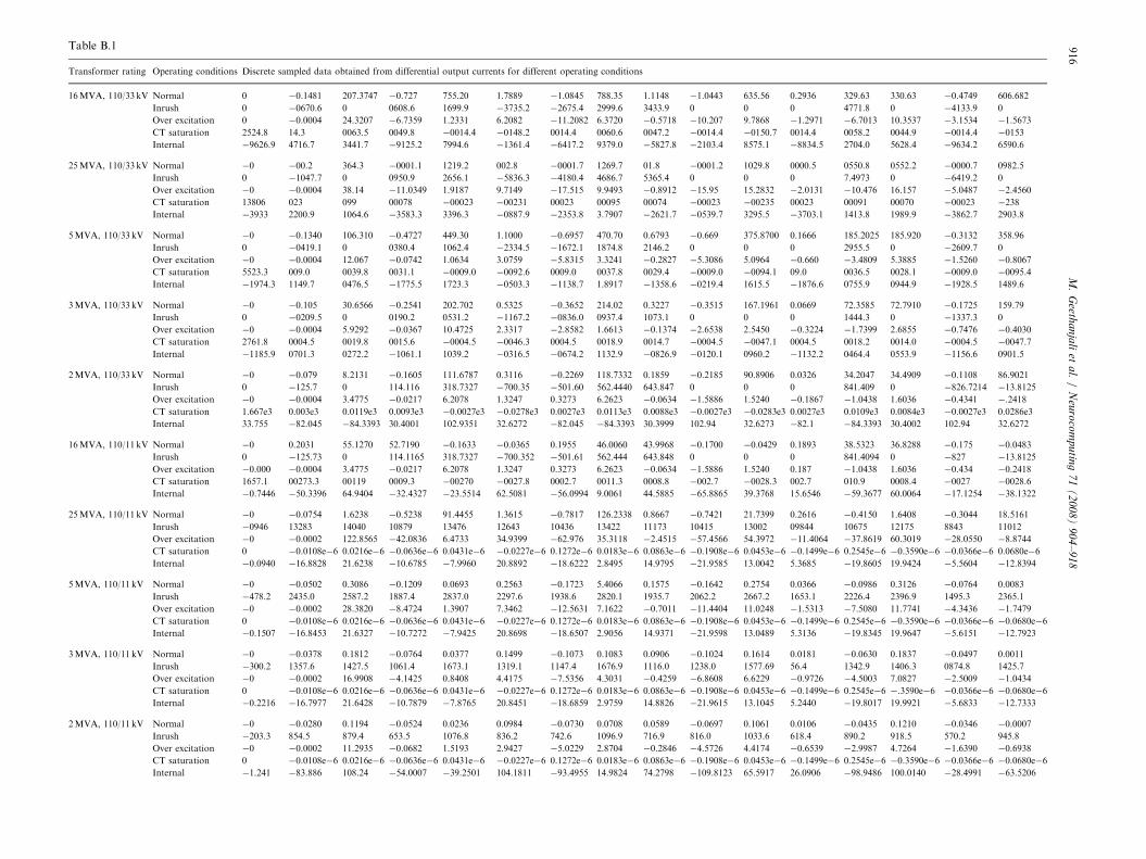
For 20 number of power transformers with different ratings(Appendix B) for the above-mentioned operating conditions thesimulated waveforms were obtained and used for the proposedscheme. For instance, the simulated waveforms obtained for a,16MVA, 110/33kV power transformer for the above men-tioned operating conditions are shown in Fig. 4(a–e).

Fig. 4. (a) Normal condition; (b) inrush current; (c) ov

5. Development of the proposed ANN model

In our proposed method the used neural network isMLFFNN. The learning process is the supervised type.The used learning paradigms are BP method and PSOtechnique. Both BP and PSO training processes require a

er excitation; (d) CT saturation; (e) internal fault.

ARTICLE IN PRESS

Fig. 4. (Continued)


ARTICLE IN PRESS

Fig. 4. (Continued)

M. Geethanjali et al. / Neurocomputing 71 (2008) 904–918910

bounded and differentiable activation functions. Therefore,sigmoid function has been used.

5.1. Development of data for training and testing

A MATLAB program has been developed for trainingprocess. The network has to discriminate the differentoperating conditions of power transformer. One hundredsets of samples (80 sets for training and 20 sets for testing)of simulated differential output current signals containing5 different operating conditions of 20 different powertransformers (given in Appendix B) were generated byusing SIMULINK model in MATLAB 6.5. Therefore,totally for each of the operating condition 20 sets ofsamples have been taken. Using FFT block, by convertingthe simulated differential output current signals intodiscrete form, 100 numbers of training sets of sampleswere generated. This signal processing is done to reduce thenumber of neural network processing element and accord-ingly it will reduce the time consumed for training andtesting of the neural network. Moreover, it also helps toachieve high performance discrimination. These signals aresampled at a sampling rate of 16 number of samples/cycle(over a data window of one cycle). These discrete sampleddata obtained for operating conditions with differentoperating conditions with different power transformerratings are tabulated in Appendix A. These 16 numbersof sampled data for each operating condition were given asinputs to the ANN architectures. The trained matrices arebuilt in such a way that the network is trained to produce a

binary output to indicate whether the measured differentialcurrent is normal, inrush, over excitation, CT saturationand internal fault.

5.2. Development of ANN architecture

ANN architecture is used so that it should recognize andclassify all the possible operating conditions of powertransformers so that it provides a trip signal whenever thefault is identified. In this proposed scheme, two differentarchitectures have been considered. One architecture is used todetect whether there is any presence of internal fault andanother for monitoring other operating conditions (which maycause maloperation of differential relay) of power transformer.The set of inputs used were 16 samples of output current

signals of power transformer. One hidden layer was takenand the number of neurons was varied from 4 to 32 andresults obtained were optimum when 32 neurons were used.The number of neurons in the hidden layer is increasedupto 64 in incremental steps. But if the number of neuronsin the hidden layer is increased, the system complexityincreases and then the results are not getting muchimproved. Various architectures were attempted to arriveat the final architecture with a goal of maximum accuracy.After many experimentations, for IFD three differentarchitectures (16-8-1, 16-16-1, 16-32-1) and for CM threedifferent architectures (16-8-4, 16-16-4, 16-32-4) weredeveloped and used for training. After enough experimen-tation, it was inferred that the architecture with one hiddenlayer of 32 neurons and one output was giving the


optimum results for IFD. And the architecture with 32neurons in the hidden layer and four outputs was giving theoptimum results for CM. Hence in the final model, anarchitecture consisting of one input layer with 16 neurons,one hidden layer with 32 neurons and one output layerwith one output (i.e. 16-32-1) was selected for IFD and thisfinal architecture is given in Fig. 6. An architectureconsisting of one input layer with 16 neurons, one hiddenlayer with 32 neurons and one output layer with fouroutputs (i.e. 16-32-4) was selected for CM. All thearchitectures were trained for 5000 iterations. Momentumfactor was kept at 0.8 throughout the work. For trainingthe network, BPN and PSO algorithms were used and theobtained simulated results for both BPN and PSO aregiven in Section 6. The architecture for detection ofinternal fault (IFD) has one output either 1 or 0. Here,the value of 0 indicates one of the non-internal faultconditions (normal, inrush, over excitation, CT saturation)and 1 indicates an internal fault. Architecture (CM) formonitoring the different operating conditions of powertransformer has four outputs.

The outputs of the network have a unique set shown asbelow:

1000—normal,0100—inrush,0010—over excitation,0001—CT saturation.

5.3. Implementations of training and testing using BP

algorithm and PSO algorithm

5.3.1. BP algorithm

The basic idea of back propagation algorithm (BPalgorithm) algorithm is using sensitivity (gradient) of theerror with respect to the weights, to conveniently modify itduring iteration steps. The paradigm realizes an optimumnonlinear mapping by associating the input trainingpatterns to the output training patterns via the successivesolutions to linear system of equations. This algorithm isdeveloped on the basis of the least squares method. For anoutput layer of ‘‘k’’ number of perceptrons the errorfunction E at the nth iteration is,

EðnÞ ¼1

2

Xk

i¼1

fTi �OiðnÞg, (4)

where T and O are the target and the actual pattern,respectively.

In this paper, the developed ANN architectures aretrained using BP algorithm. In other words, the weightadjustments of neural network neurons are done usingerror BP method.

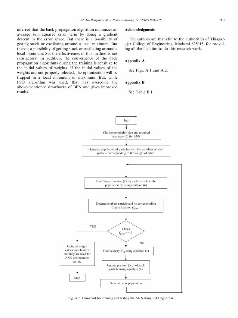
5.3.2. PSO algorithm

PSO is initialized with a group of random particles(solutions) and then searches for optima by updating

generations. In every iteration, each particle is updated bytwo ‘‘best’’ values namely pbest and gbest. After finding thetwo best values, the particle updates its velocity andpositions with Eqs. (2) and (3).The objective function (i.e. fitness function) is

f ¼Xp

½ðtargetÞ � ðactual outputÞ�2. (5)

The inertia weight value selected is 0.9. The values of bothc1 and c2 are taken as 1.75.The fitness function for each particle is obtained by

updating the weights of ANN as specified by the variablesof the particle and finding the mean squared error obtainedin ANN training as per Eq. (5). Similarly, the fitnessfunctions of all particles in the population are determined.The particle having lowest fitness function is the gbest

particle and the fitness function of the gbest particle iscompared with the specified accuracy. If the requiredaccuracy is obtained then the training is stopped. Other-wise, the velocity and new position of the particles areupdated as per Eqs. (2) and (3). The same process isrepeated until the specified accuracy is reached.

6. Simulated results and analysis

Since the weight adjustment of neurons is nonlinear anddynamic, this paper uses the PSO algorithm to adjust theset of weights. The velocity and position of the particles areadjusted to find the optimal value of weights that meet apre-specified mean squared error. The initial populationsize of 20 particles is selected. Particles inside thepopulation are drawn gradually towards the globalminimum as the system iterates. When the pre-specifiederror criterion is reached, the iterations cease and the set ofthese optimized weights found is finalized and used in theproposed architecture.The detailed flowcharts of the implementations of BP

algorithm and PSO algorithm for training and testing theproposed ANN architectures are given in Appendix A.Thus, the discrimination of different operating condi-

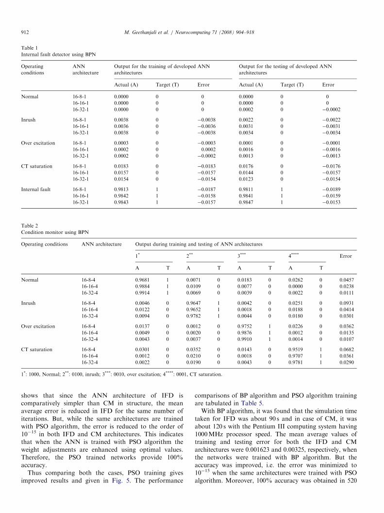
tions for power transformers is carried out by ANN trainedwith BP and PSO algorithms using the waveforms obtainedfor practical power transformers and the results areanalyzed. The detailed simulated results for BPN trainingof IFD and CM architectures are given in Tables 1 and 2.The detailed simulated results for PSO training of IFD andCM architectures are given in Tables 3 and 4.After enough training, ANN model was tested with all

the possible sets of data under different operatingconditions of the power transformer by using both BPand PSO algorithms. The network was tested to checkwhether the corresponding indication was given. If internalfault occurred IFD issues a trip signal. If internal fault doesnot occur then the condition of the power transformer ismonitored using 4-output network.While training with BP algorithm for IFD, the mean

average error is 0.009225 and for CM, it is 0.036575. It

ARTICLE IN PRESS

Table 2

Condition monitor using BPN

Operating conditions ANN architecture Output during training and testing of ANN architectures

1* 2** 3*** 4**** Error

A T A T A T A T

Normal 16-8-4 0.9681 1 0.0071 0 0.0183 0 0.0262 0 0.0457

16-16-4 0.9884 1 0.0109 0 0.0077 0 0.0000 0 0.0238

16-32-4 0.9914 1 0.0069 0 0.0039 0 0.0022 0 0.0111

Inrush 16-8-4 0.0046 0 0.9647 1 0.0042 0 0.0251 0 0.0931

16-16-4 0.0122 0 0.9652 1 0.0018 0 0.0188 0 0.0414

16-32-4 0.0094 0 0.9782 1 0.0044 0 0.0180 0 0.0301

Over excitation 16-8-4 0.0137 0 0.0012 0 0.9752 1 0.0226 0 0.0362

16-16-4 0.0049 0 0.0020 0 0.9876 1 0.0012 0 0.0135

16-32-4 0.0043 0 0.0037 0 0.9910 1 0.0014 0 0.0107

CT saturation 16-8-4 0.0301 0 0.0352 0 0.0143 0 0.9519 1 0.0682

16-16-4 0.0012 0 0.0210 0 0.0018 0 0.9707 1 0.0361

16-32-4 0.0022 0 0.0190 0 0.0043 0 0.9781 1 0.0290

1*: 1000, Normal; 2**: 0100, inrush; 3***: 0010, over excitation; 4****: 0001, CT saturation.

Table 1

Internal fault detector using BPN

Operating

conditions

ANN

architecture

Output for the training of developed ANN

architectures

Output for the testing of developed ANN

architectures

Actual (A) Target (T) Error Actual (A) Target (T) Error

Normal 16-8-1 0.0000 0 0 0.0000 0 0

16-16-1 0.0000 0 0 0.0000 0 0

16-32-1 0.0000 0 0 0.0002 0 �0.0002

Inrush 16-8-1 0.0038 0 �0.0038 0.0022 0 �0.0022

16-16-1 0.0036 0 �0.0036 0.0031 0 �0.0031

16-32-1 0.0038 0 �0.0038 0.0034 0 �0.0034

Over excitation 16-8-1 0.0003 0 �0.0003 0.0001 0 �0.0001

16-16-1 0.0002 0 0.0002 0.0016 0 �0.0016

16-32-1 0.0002 0 �0.0002 0.0013 0 �0.0013

CT saturation 16-8-1 0.0183 0 �0.0183 0.0176 0 �0.0176

16-16-1 0.0157 0 �0.0157 0.0144 0 �0.0157

16-32-1 0.0154 0 �0.0154 0.0123 0 �0.0154

Internal fault 16-8-1 0.9813 1 �0.0187 0.9811 1 �0.0189

16-16-1 0.9842 1 �0.0158 0.9841 1 �0.0159

16-32-1 0.9843 1 �0.0157 0.9847 1 �0.0153


shows that since the ANN architecture of IFD iscomparatively simpler than CM in structure, the meanaverage error is reduced in IFD for the same number ofiterations. But, while the same architectures are trainedwith PSO algorithm, the error is reduced to the order of10�15 in both IFD and CM architectures. This indicatesthat when the ANN is trained with PSO algorithm theweight adjustments are enhanced using optimal values.Therefore, the PSO trained networks provide 100%accuracy.

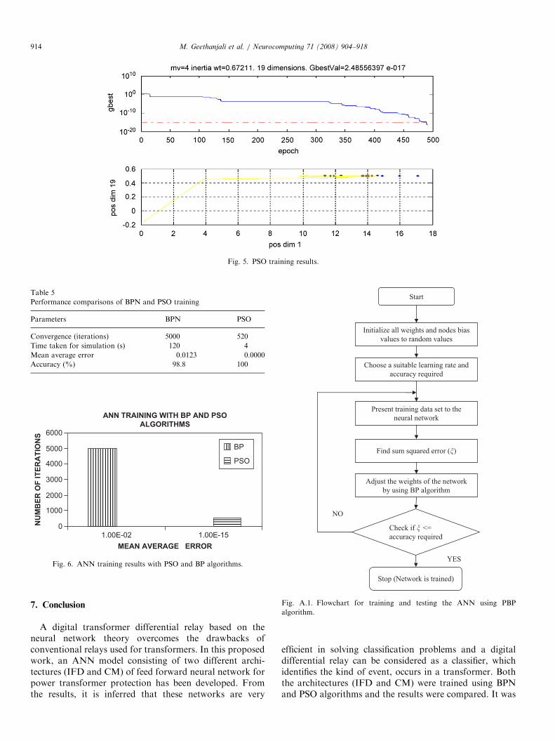
Thus comparing both the cases, PSO training givesimproved results and given in Fig. 5. The performance

comparisons of BP algorithm and PSO algorithm trainingare tabulated in Table 5.With BP algorithm, it was found that the simulation time

taken for IFD was about 90 s and in case of CM, it wasabout 120 s with the Pentium III computing system having1000MHz processor speed. The mean average values oftraining and testing error for both the IFD and CMarchitectures were 0.001623 and 0.00325, respectively, whenthe networks were trained with BP algorithm. But theaccuracy was improved, i.e. the error was minimized to10�15 when the same architectures were trained with PSOalgorithm. Moreover, 100% accuracy was obtained in 520

ARTICLE IN PRESS

Table 4

Condition monitor using PSO

Operating conditions ANN architecture Output during training and testing of ANN architectures

1* 2** 3*** 4**** Error

A T A T A T A T

Normal 16-8-4 1 1 0 0 0 0 0 0 0

16-16-4 1 1 0 0 0 0 0 0 0

16-32-4 1 1 0 0 0 0 0 0 0

Inrush 16-8-4 0 0 1 1 0 0 0 0 0

16-16-4 0 0 1 1 0 0 0 0 0

16-32-4 0 0 1 1 0 0 0 0 0

Over excitation 16-8-4 0 0 0 0 1 1 0 0 0

16-16-4 0 0 0 0 1 1 0 0 0

16-32-4 0 0 0 0 1 1 0 0 0

CT saturation 16-8-4 0 0 0 0 0 0 1 1 0

16-16-4 0 0 0 0 0 0 1 1 0

16-32-4 0 0 0 0 0 0 1 1 0

1*: 1000, Normal; 2**: 0100, inrush; 3***: 0010, over excitation; 4****: 0001, CT saturation.

Table 3

Internal fault detector using PSO

Operating

conditions

ANN

architecture

Output for the training of developed ANN

architectures

Output for the testing of developed ANN

architectures

Actual (A) Target (T) Error Actual (A) Target (T) Error

Normal 16-8-1 0.0000 0 0 0.0000 0 0

16-16-1 0.0000 0 0 0.0000 0 0

16-32-1 0.0000 0 0 0.0000 0 0

Inrush 16-8-1 0.0000 0 0 0.0000 0 0

16-16-1 0.0000 0 0 0.0000 0 0

16-32-1 0.0000 0 0 0.0000 0 0

Over excitation 16-8-1 0.0000 0 0 0.0000 0 0

16-16-1 0.0000 0 0 0.0000 0 0

16-32-1 0.0000 0 0 0.0000 0 0

CT saturation 16-8-1 0.0000 0 0 0.0000 0 0

16-16-1 0.0000 0 0 0.0000 0 0

16-32-1 0.0000 0 0 0.0000 0 0

Internal fault 16-8-1 1.0000 1 0 1.0000 1 0

16-16-1 1.0000 1 0 1.0000 1 0

16-32-1 1.0000 1 0 1.0000 1 0


epochs itself. The simulation time taken for PSO trainingwas also reduced to 4 s. As shown in Fig. 6, an error of 10�15

has been reached by using PSO algorithm after an averageof 520 iterations in the training phase. But in about 5000iterations, the mean squared error reached by using backpropagation algorithm is about 10�2. In Ref. [4], the PSOtrained ANN was able to discriminate between inrush andinternal fault current waveforms with an accuracy of about95%. But the proposed scheme was able to discriminateamong four different conditions with 100% accuracy.

Thus comparing the simulation results of both thecases, PSO trained neural network architecture gives moreaccurate (in terms of least sum square error) and also fasterresults (in terms of number of iterations required to reach apre-specified error criterion and simulation time). Thus,the proposed ANN-based differential relaying for powertransformer gives promising security (ability to not tripwhen it should not), dependability (ability to trip when itshould) and speed of operation (short fault clearingtime).

ARTICLE IN PRESS

ANN TRAINING WITH BP AND PSO

ALGORITHMS

0

1000

2000

3000

4000

5000

6000

1.00E-02 1.00E-15

MEAN AVERAGE ERROR

NU

MB

ER

OF

IT

ER

AT

ION

S

BP

PSO

Fig. 6. ANN training results with PSO and BP algorithms.

Table 5

Performance comparisons of BPN and PSO training

Parameters BPN PSO

Convergence (iterations) 5000 520

Time taken for simulation (s) 120 4

Mean average error 0.0123 0.0000

Accuracy (%) 98.8 100

Fig. 5. PSO training results.

Start

Initialize all weights and nodes bias

values to random values

Choose a suitable learning rate and

accuracy required

Present training data set to the

neural network

Find sum squared error (�)

Adjust the weights of the network

by using BP algorithm

Stop (Network is trained)

Check if � <=

accuracy required

YES

NO

Fig. A.1. Flowchart for training and testing the ANN using PBP

algorithm.


7. Conclusion

A digital transformer differential relay based on theneural network theory overcomes the drawbacks ofconventional relays used for transformers. In this proposedwork, an ANN model consisting of two different archi-tectures (IFD and CM) of feed forward neural network forpower transformer protection has been developed. Fromthe results, it is inferred that these networks are very

efficient in solving classification problems and a digitaldifferential relay can be considered as a classifier, whichidentifies the kind of event, occurs in a transformer. Boththe architectures (IFD and CM) were trained using BPNand PSO algorithms and the results were compared. It was


inferred that the back propagation algorithm minimizes anaverage sum squared error term by doing a gradientdescent in the error space. But there is a possibility ofgetting stuck or oscillating around a local minimum. Butthere is a possibility of getting stuck or oscillating around alocal minimum. So, the effectiveness of this method is notsatisfactory. In addition, the convergence of the backpropagation algorithms during the training is sensitive tothe initial values of weights. If the initial values of theweights are not properly selected, the optimization will betrapped in a local minimum or maximum. But, whilePSO algorithm was used, that has overcome theabove-mentioned drawbacks of BPN and gives improvedresults.

S

Choose populati

accuracy

Generate population of part

particle correspondin

Find fitness function (

population by u

Determine gbest parti

fitness fun

Find velocity Vid

C

fgbes

Update positi

particle usin

Generate ne

Optimal weight

values are obtained

and they are used for

ANN architectures

testing

Stop

YES

Fig. A.2. Flowchart for training and tes

Acknowledgments

The authors are thankful to the authorities of Thiagar-ajar College of Engineering, Madurai 625015, for provid-ing all the facilities to do this research work.

Appendix A

See Figs. A.1 and A.2.

Appendix B

See Table B.1.

tart

on size and required

(�) for ANN

icles with the variables of each

g to the weight of ANN

f ) for each particle in the

sing equation (6)

cle and its corresponding

ction (fgbest)

using equation (3)

heck

t <= �

on (Xid) of each

g equation (4)

w population

NO

ting the ANN using PSO algorithm.

ARTIC

LEIN

PRES

STable B.1

Transformer rating Operating conditions Discrete sampled data obtained from differential output currents for different operating conditions

16MVA, 110/33 kV Normal 0 �0.1481 207.3747 �0.727 755.20 1.7889 �1.0845 788.35 1.1148 �1.0443 635.56 0.2936 329.63 330.63 �0.4749 606.682

Inrush 0 �0670.6 0 0608.6 1699.9 �3735.2 �2675.4 2999.6 3433.9 0 0 0 4771.8 0 �4133.9 0

Over excitation 0 �0.0004 24.3207 �6.7359 1.2331 6.2082 �11.2082 6.3720 �0.5718 �10.207 9.7868 �1.2971 �6.7013 10.3537 �3.1534 �1.5673

CT saturation 2524.8 14.3 0063.5 0049.8 �0014.4 �0148.2 0014.4 0060.6 0047.2 �0014.4 �0150.7 0014.4 0058.2 0044.9 �0014.4 �0153

Internal �9626.9 4716.7 3441.7 �9125.2 7994.6 �1361.4 �6417.2 9379.0 �5827.8 �2103.4 8575.1 �8834.5 2704.0 5628.4 �9634.2 6590.6

25MVA, 110/33 kV Normal �0 �00.2 364.3 �0001.1 1219.2 002.8 �0001.7 1269.7 01.8 �0001.2 1029.8 0000.5 0550.8 0552.2 �0000.7 0982.5

Inrush 0 �1047.7 0 0950.9 2656.1 �5836.3 �4180.4 4686.7 5365.4 0 0 0 7.4973 0 �6419.2 0

Over excitation �0 �0.0004 38.14 �11.0349 1.9187 9.7149 �17.515 9.9493 �0.8912 �15.95 15.2832 �2.0131 �10.476 16.157 �5.0487 �2.4560

CT saturation 13806 023 099 00078 �00023 �00231 00023 00095 00074 �00023 �00235 00023 00091 00070 �00023 �238

Internal �3933 2200.9 1064.6 �3583.3 3396.3 �0887.9 �2353.8 3.7907 �2621.7 �0539.7 3295.5 �3703.1 1413.8 1989.9 �3862.7 2903.8

5MVA, 110/33 kV Normal �0 �0.1340 106.310 �0.4727 449.30 1.1000 �0.6957 470.70 0.6793 �0.669 375.8700 0.1666 185.2025 185.920 �0.3132 358.96

Inrush 0 �0419.1 0 0380.4 1062.4 �2334.5 �1672.1 1874.8 2146.2 0 0 0 2955.5 0 �2609.7 0

Over excitation �0 �0.0004 12.067 �0.0742 1.0634 3.0759 �5.8315 3.3241 �0.2827 �5.3086 5.0964 �0.660 �3.4809 5.3885 �1.5260 �0.8067

CT saturation 5523.3 009.0 0039.8 0031.1 �0009.0 �0092.6 0009.0 0037.8 0029.4 �0009.0 �0094.1 09.0 0036.5 0028.1 �0009.0 �0095.4

Internal �1974.3 1149.7 0476.5 �1775.5 1723.3 �0503.3 �1138.7 1.8917 �1358.6 �0219.4 1615.5 �1876.6 0755.9 0944.9 �1928.5 1489.6

3MVA, 110/33 kV Normal �0 �0.105 30.6566 �0.2541 202.702 0.5325 �0.3652 214.02 0.3227 �0.3515 167.1961 0.0669 72.3585 72.7910 �0.1725 159.79

Inrush 0 �0209.5 0 0190.2 0531.2 �1167.2 �0836.0 0937.4 1073.1 0 0 0 1444.3 0 �1337.3 0

Over excitation �0 �0.0004 5.9292 �0.0367 10.4725 2.3317 �2.8582 1.6613 �0.1374 �2.6538 2.5450 �0.3224 �1.7399 2.6855 �0.7476 �0.4030

CT saturation 2761.8 0004.5 0019.8 0015.6 �0004.5 �0046.3 0004.5 0018.9 0014.7 �0004.5 �0047.1 0004.5 0018.2 0014.0 �0004.5 �0047.7

Internal �1185.9 0701.3 0272.2 �1061.1 1039.2 �0316.5 �0674.2 1132.9 �0826.9 �0120.1 0960.2 �1132.2 0464.4 0553.9 �1156.6 0901.5

2MVA, 110/33 kV Normal �0 �0.079 8.2131 �0.1605 111.6787 0.3116 �0.2269 118.7332 0.1859 �0.2185 90.8906 0.0326 34.2047 34.4909 �0.1108 86.9021

Inrush 0 �125.7 0 114.116 318.7327 �700.35 �501.60 562.4440 643.847 0 0 0 841.409 0 �826.7214 �13.8125

Over excitation �0 �0.0004 3.4775 �0.0217 6.2078 1.3247 0.3273 6.2623 �0.0634 �1.5886 1.5240 �0.1867 �1.0438 1.6036 �0.4341 �.2418

CT saturation 1.667e3 0.003e3 0.0119e3 0.0093e3 �0.0027e3 �0.0278e3 0.0027e3 0.0113e3 0.0088e3 �0.0027e3 �0.0283e3 0.0027e3 0.0109e3 0.0084e3 �0.0027e3 0.0286e3

Internal 33.755 �82.045 �84.3393 30.4001 102.9351 32.6272 �82.045 �84.3393 30.3999 102.94 32.6273 �82.1 �84.3393 30.4002 102.94 32.6272

16MVA, 110/11 kV Normal �0 0.2031 55.1270 52.7190 �0.1633 �0.0365 0.1955 46.0060 43.9968 �0.1700 �0.0429 0.1893 38.5323 36.8288 �0.175 �0.0483

Inrush 0 �125.73 0 114.1165 318.7327 �700.352 �501.61 562.444 643.848 0 0 0 841.4094 0 �827 �13.8125

Over excitation �0.000 �0.0004 3.4775 �0.0217 6.2078 1.3247 0.3273 6.2623 �0.0634 �1.5886 1.5240 0.187 �1.0438 1.6036 �0.434 �0.2418

CT saturation 1657.1 00273.3 00119 0009.3 �00270 �0027.8 0002.7 0011.3 0008.8 �002.7 �0028.3 002.7 010.9 0008.4 �0027 �0028.6

Internal �0.7446 �50.3396 64.9404 �32.4327 �23.5514 62.5081 �56.0994 9.0061 44.5885 �65.8865 39.3768 15.6546 �59.3677 60.0064 �17.1254 �38.1322

25MVA, 110/11 kV Normal �0 �0.0754 1.6238 �0.5238 91.4455 1.3615 �0.7817 126.2338 0.8667 �0.7421 21.7399 0.2616 �0.4150 1.6408 �0.3044 18.5161

Inrush �0946 13283 14040 10879 13476 12643 10436 13422 11173 10415 13002 09844 10675 12175 8843 11012

Over excitation �0 �0.0002 122.8565 �42.0836 6.4733 34.9399 �62.976 35.3118 �2.4515 �57.4566 54.3972 �11.4064 �37.8619 60.3019 �28.0550 �8.8744

CT saturation 0 �0.0108e�6 0.0216e�6 �0.0636e�6 0.0431e�6 �0.0227e�6 0.1272e�6 0.0183e�6 0.0863e�6 �0.1908e�6 0.0453e�6 �0.1499e�6 0.2545e�6 �0.3590e�6 �0.0366e�6 0.0680e�6

Internal �0.0940 �16.8828 21.6238 �10.6785 �7.9960 20.8892 �18.6222 2.8495 14.9795 �21.9585 13.0042 5.3685 �19.8605 19.9424 �5.5604 �12.8394

5MVA, 110/11 kV Normal �0 �0.0502 0.3086 �0.1209 0.0693 0.2563 �0.1723 5.4066 0.1575 �0.1642 0.2754 0.0366 �0.0986 0.3126 �0.0764 0.0083

Inrush �478.2 2435.0 2587.2 1887.4 2837.0 2297.6 1938.6 2820.1 1935.7 2062.2 2667.2 1653.1 2226.4 2396.9 1495.3 2365.1

Over excitation �0 �0.0002 28.3820 �8.4724 1.3907 7.3462 �12.5631 7.1622 �0.7011 �11.4404 11.0248 �1.5313 �7.5080 11.7741 �4.3436 �1.7479

CT saturation 0 �0.0108e�6 0.0216e�6 �0.0636e�6 0.0431e�6 �0.0227e�6 0.1272e�6 0.0183e�6 0.0863e�6 �0.1908e�6 0.0453e�6 �0.1499e�6 0.2545e�6 �0.3590e�6 �0.0366e�6 �0.0680e�6

Internal �0.1507 �16.8453 21.6327 �10.7272 �7.9425 20.8698 �18.6507 2.9056 14.9371 �21.9598 13.0489 5.3136 �19.8345 19.9647 �5.6151 �12.7923

3MVA, 110/11 kV Normal �0 �0.0378 0.1812 �0.0764 0.0377 0.1499 �0.1073 0.1083 0.0906 �0.1024 0.1614 0.0181 �0.0630 0.1837 �0.0497 0.0011

Inrush �300.2 1357.6 1427.5 1061.4 1673.1 1319.1 1147.4 1676.9 1116.0 1238.0 1577.69 56.4 1342.9 1406.3 0874.8 1425.7

Over excitation �0 �0.0002 16.9908 �4.1425 0.8408 4.4175 �7.5356 4.3031 �0.4259 �6.8608 6.6229 �0.9726 �4.5003 7.0827 �2.5009 �1.0434

CT saturation 0 �0.0108e�6 0.0216e�6 �0.0636e�6 0.0431e�6 �0.0227e�6 0.1272e�6 0.0183e�6 0.0863e�6 �0.1908e�6 0.0453e�6 �0.1499e�6 0.2545e�6 �.3590e�6 �0.0366e�6 �0.0680e�6

Internal �0.2216 �16.7977 21.6428 �10.7879 �7.8765 20.8451 �18.6859 2.9759 14.8826 �21.9615 13.1045 5.2440 �19.8017 19.9921 �5.6833 �12.7333

2MVA, 110/11 kV Normal �0 �0.0280 0.1194 �0.0524 0.0236 0.0984 �0.0730 0.0708 0.0589 �0.0697 0.1061 0.0106 �0.0435 0.1210 �0.0346 �0.0007

Inrush �203.3 854.5 879.4 653.5 1076.8 836.2 742.6 1096.9 716.9 816.0 1033.6 618.4 890.2 918.5 570.2 945.8

Over excitation �0 �0.0002 11.2935 �0.0682 1.5193 2.9427 �5.0229 2.8704 �0.2846 �4.5726 4.4174 �0.6539 �2.9987 4.7264 �1.6390 �0.6938


Internal �1.241 �83.886 108.24 �54.0007 �39.2501 104.1811 �93.4955 14.9824 74.2798 �109.8123 65.5917 26.0906 �98.9486 100.0140 �28.4991 �63.5206

M.

Geeth

an

jali

eta

l./

Neu

roco

mpu

ting

71

(2

00

8)

90

4–

91

8916

ARTIC

LEIN

PRES

S16MVA, 66/33 kV Normal �0 �0.0793 131.0846 �0.9142 862.2454 2.4309 �1.3855 910.103 1.5387 �1.3268 710.7748 0.4511 307.3426 309.1715 �0.5670 678.8184

Inrush �.4530e4 1.2551e4 1.2241e4 0.6906e4 1.6196e4 1.0769e4 0.8815e4 1.6751e4 0.8366e4 1.0756e4 1.5647e4 0.6528e4 1.2743e4 1.3408e4 0.5810e4 1.4297e4

Over excitation �0 �0.0002 6.6611 �0.0455 13.6891 1.0649 �3.5265 2.4933 �0.1277 �4.0589 3.7581 �0.3105 �2.6646 3.7431 �0.7358 �0.6283


Internal �0.8103 �84.1757 108.1736 �53.6302 �39.6560 104.3319 �93.2792 14.5581 74.6051 �109.8026 65.2528 26.5169 �99.1490 99.8470 �28.0837 �63.8843

25MVA, 66/33 kV Normal �0 �1 227.3 �001.4 1368.9 3.8 �0.002.1 1442.9 2.4 �02.1 1130.6 007 499.5 502.3 �0000.9 1079.2

Inrush �0.6976e4 2.0649e4 2.0914e4 1.2096e4 2.6241e4 1.8033e4 1.4318e4 2.6731e4 1.3857e4 1.6988e4 2.4959e4 1.0741e4 1.9971e4 2.1506e4 0.9415e4 2.2403e4

Over excitation �0 �0.0002 10.4663 �0.0712 2.2303 1.6150 �5.5267 3.8945 �0.1999 �6.3433 5.8706 �0.4844 �4.1652 5.8434 �1.1450 �0.9839

CT saturation 0 �0.0054e�5 0.0108e�5 �0.0318e�5 �0.0216e�5 �0.0113e�5 0.0636e�5 0.0092e�5 0.0431e�5 �0.0954e�5 0.0227e�5 �0.0749e�5 0.1272e�5 �0.1795e�5 �0.0183e�5 �0.0340e�5

Internal �3.8658 �82.0555 108.5445 �56.2132 �36.7450 103.1914 �94.7449 17.5588 72.2311 �109.7901 67.6145 23.5137 �97.6594 100.9611 �30.9896 �61.2906

5MVA, 66/33 kV Normal �0 �0.0690 16.9217 �0.3047 246.0252 0.7411 �0.4510 261.6568 0.4628 �0.4321 200.0166 0.1234 74.5090 75.1455 �0.1941 191.203


Over excitation �0 �0.0002 2.0120 �0.0140 4.2151 0.3315 �0.0369 4.2927 �0.0381 0.9017 3.6089 �0.0613 0.6648 1.1844 �0.2238 �0.1954


Internal �6.3924 �80.2065 108.7220 �58.2925 �34.2948 102.1233 �95.8436 20.0222 70.1781 �109.6490 69.4840 20.9966 �96.3090 101.7644 �33.3596 �59.0722

3MVA, 66/33 kV Normal �0.0000 �0.0609 0.5252 �0.1915 136.7723 0.4362 �0.2790 146.4270 0.2693 �0.2683 109.7107 0.0659 34.6398 35.0451 �0.1244 104.906


Over excitation �0.0000 �0.0002 1.1688 �0.0083 2.4925 0.1628 �0.0218 2.5412 �0.0223 0.5082 2.1329 �0.0360 1.3542 1.3509 �0.0489 2.0084

CT saturation 0 �0.0054e�5 0.0108e�5 �0.0318e�5 .0216e�5 �0.0113e�5 0.0636e�5 0.0092e�5 0.0431e�5 �0.0954e�5 0.0227e�5 �0.0749e�5 0.1272e�5 �0.1795e�5 �0.0183e�5 �0.0340e�5

Internal �9.5131 �77.7945 108.7794 �60.7735 �31.2031 100.6471 �97.0655 23.0467 67.5355 �109.3079 71.7023 17.8495 �94.4901 102.6097 �36.2473 �56.2406

2MVA, 66/33 kV Normal �0.0000 �0.0526 0.3444 �0.1333 84.1997 0.2853 �0.1905 90.8046 0.1741 �0.1842 66.4883 0.0386 16.5860 16.8673 �0.0881 63.5830


Over excitation �0.0000 �0.0002 0.7491 �0.0054 1.6328 0.0800 �0.0142 1.6667 �0.0145 0.3125 1.3959 �0.0234 0.8777 0.8757 �0.0318 13151


Internal �0.3842 �56.2217 72.0909 �35.6188 �26.5826 69.6101 �62.1055 9.5519 49.8559 �73.1977 43.3801 17.8271 �66.1716 66.5039 �18.5738 �42.7174

16MVA, 66/22 kV Normal �0.3842 �56.2217 72.0909 �35.6188 �26.5826 69.6101 �62.1055 9.5519 49.8559 �73.1977 43.3801 17.8271 �66.1716 66.5039 �18.5738 �42.7174

Inrush �0.0000 �0.0793 131.0852 �0.9142 862.2472 2.4309 �1.3856 910.1059 1.5388 �1.3275 710.7784 0.4509 307.3464 309.1760 �0.5670 678.8235

Over excitation �0.4358e4 1.3806e4 1.4320e4 0.8275e4 1.7019e4 1.2055e4 0.9265e4 1.7230e4 0.9250e4 1.0826e4 1.6165e4 0.7158e4 1.2686e4 1.4039e4 0.6189e4 1.4256e4

CT saturation �0.0000 �0.0002 18.9047 �4.1672 1.1055 4.4623 �10.0395 5.6832 �0.4031 �9.1427 8.6707 �0.9466 �6.0009 8.9922 �2.1905 �1.4051

Internal 0 �0.0036e�5 0.0072e�5 �0.0212e�5 0.0144e�5 �0.0076e�5 0.0424e�5 0.0061e�5 0.0288e�5 �0.0636e�5 0.0151e�5 �0.0500e�5 0.0848e�5 �0.1197e�5 �0.0122e�5 �0.0227e�5

25MVA, 66/22 kV Normal �0.2564 �56.3053 72.0717 �35.5104 �26.7011 69.6533 �62.0415 9.4281 49.9535 �73.1952 43.2776 17.9541 �66.2303 66.4526 �18.4501 �42.8246

Inrush �0.0000 �0.0001e3 0.2273e3 �0.0014e3 1.3689e3 0.0038e3 �.0021e3 1.4429e3 0.0024e3 �0.0021e3 1.1306e3 0.0007e3 0.4995e3 0.5023e3 �.0009e3 1.0792e3

Over excitation �0.6401e4 2.2578e4 2.3908e4 1.3646e4 2.6494e4 1.9759e4 1.4515e4 2.6887e4 1.5309e4 1.6660e4 2.5495e4 1.187e4 1.9415e4 22450 1.0085e4 2.1872e4

CT saturation �0.0000 �0.0002 29.5923 �7.3624 1.7144 6.9316 �15.6906 8.8667 �0.6218 �14.2923 13.5254 �1.4507 �9.3860 13.9857 �3.3374 �2.2080


5MVA, 66/22 kV Normal �1.1639 �55.6934 72.2030 �36.2883 �25.8451 69.3345 �62.4935 10.3198 49.2599 �73.2120 43.9914 17.0637 �65.8073 66.8018 �19.3189 �42.0643

Inrush �0.0000 �0.0690 16.9225 �0.3047 246.0292 0.7410 �0.4514 261.6610 0.4628 �0.4323 200.0205 0.1234 74.5111 75.1466 �0.1942 191.2055


CT saturation �0.0000 �0.0002 5.8373 �0.0369 10.7405 1.9857 �3.0720 1.7783 �0.1259 �2.8553 2.7123 �0.2984 �1.8729 2.8181 �0.6963 �0.4362


3MVA 66/22 kV Normal �1.9185 �55.1697 72.2946 �36.9268 �25.1273 69.0515 �62.8572 11.0596 48.6741 �73.2081 44.5768 16.3229 �65.4387 67.0788 �20.0353 �41.4281

Inrush �0.0000 �0.0609 0.5252 �0.1916 136.7727 0.4360 �0.2793 146.4280 0.2693 �0.2678 109.7100 0.0659 34.6388 35.0427 �0.1245 104.9048


CT saturation �0.0000 �0.0002 3.4618 �0.0220 6.4081 1.1564 0.0881 6.4777 �0.0633 �1.7116 1.6264 �0.1767 �1.1234 1.6892 �0.4133 �0.2614


2MVA 66/22 kV Normal �2.8589 �54.5025 72.3873 �37.7132 �24.2274 68.6802 �63.2901 11.9802 47.9280 �73.1831 45.2889 15.3967 �64.9615 67.4026 �20.9248 �40.6144

Inrush �0.0000 �0.0526 0.3444 �0.1333 84.2016 0.2851 �0.1915 90.8060 0.1741 �0.1839 66.4893 0.0386 16.5872 16.8676 �0.0881 63.5835


CT saturation �0.0000 �0.0002 2.2748 �0.0146 4.2412 0.7407 0.0299 4.2902 �0.0417 1.2233 3.6553 �0.0659 �0.6273 1.1281 �0.2708 �0.1740


M.

Geeth

an

jali

eta

l./

Neu

roco

mpu

ting

71

(2

00

8)

90

4–

91

8917


References

[1] A.I. Elgallad, M. El-Hawary, A.A. Sallam, A. Kalas, Swarm

intelligently trained neural network for power transformer protec-

tion, in: Proceedings of Canadian Conference on Electrical and

Computer Engineering, vol. 1, 2001, pp. 265–269, Website link:

/http://ieeexplore.ieee.orgS.

[2] S. Kannan, S. Mary Raja Slochanal, P. Subburaj, N.P. Padhy,

Application of particle swarm optimization technique and its variants

to generation expansion planning problem, Electr. Power Syst. Res.

70 (2004) 203–210.

[3] P. Liu, O.P. Malik, D. Chen, G.S. Hope, Y. Guo, Improved

operation of differential protection of power transformers for internal

faults, IEEE Trans. Power Deliv. 7 (4) (1992) 1912.

[4] Z. Moravej, D.N. Vishwakarma, ANN-based harmonic restraint

differential protection of power transformer, IE J. 84 (2003) 1–6.

[5] Z. Moravej, D.N. Vishwakarma, S.P. Singh, Applicability of artificial

neural networks to power transformer protection—an overview, in:

Proceedings of 14th National Convention of Electrical Engineering,

1998, p. 230.

[6] Z. Moravej, D.N. Vishwakarma, S.P. Singh, ANN based protec-

tion for power transformers, Electr. Mach. Power Syst. 28 (2000)

875–884.

[7] Z. Moravej, D.N. Vishwakarma, S.P. Singh, Radial basis function

neural network model for protection of power transformers, Electr.

Power Comp. Syst. 29 (2001) 307–320.

[8] Z. Moravej, D.N. Vishwakarma, S.P. Singh, Protection and

condition monitoring of power transformer using ANN, Electr.

Power Comp. Syst. 30 (2002) 217–231.

[9] J. Philer, B. Grcar, D. Dolinar, Improved operation of power

transformer protection using ANN, IEEE Trans. Power Deliv. 12 (3)

(1997) 1128–1136.

[10] R.L. Sharp, W.E. Glassburn, A transformer differential relay with

second harmonic restraint, Trans. Am. Inst. Electr. Eng. 77 (1985)

884.

[11] J.A. Sykes, I.F. Morrison, A proposed method of harmonic restraint

differential protection of transformers by digital computer, IEEE

Trans. Power Apparatus Syst. PAS-91 (3) (1972) 1266.

[12] Tamil Nadu Electricity Board Statistics at a Glance 2003–2004,

Planning Wing of Tamil Nadu Electricity Board, Chennai, India.

M. Geethanjali obtained her BE degree in

electrical engineering in 1989 and Master’s degree

in power systems engineering in 1991 from

Thiagarajar College of Engineering, Madurai,

India. She has been in teaching for the past 15

years. She is presently working as a lecturer in

electrical engineering in Thiagarajar College of

Engineering, Madurai. She is now working

towards her Ph.D. Her field of interest is power

system protection and control.

S. Mary Raja Slochanal received the BE degree in

electrical engineering in 1981, the Master’s degree

in power systems engineering (with distinction) in

1985, and the Ph.D. degree in power systems in

1997, all from Thiagarajar College of Engineer-

ing, Madurai, India. She has been involved in

teaching for the past 20 years. She is currently a

professor of electrical engineering at Thiagarajar

College of Engineering. She has published 65

research papers. Her fields of interests are power system modeling,

FACTS, reliability, and wind energy.

R. Bhavani received her Master’s degree in power systems engineering

in Thiagarajar College of Engineering, Madurai, in 2005. Presently,

she is working as a lecturer in P.S.N.A. College of Engineering and

Technology, Dindigul, India. Her field of interest is digital power system

protection.

http://ieeexplore.ieee.org

pso trained ann-based differential protection scheme...

Documents